Embed Size (px)
Citation preview

Louisiana State UniversityLSU Digital Commons
LSU Doctoral Dissertations Graduate School
2005
Parallel molecular dynamics simulations ofpressure-induced structural transformations incadmium selenide nanocrystalsNicholas Jabari Ouma LeeLouisiana State University and Agricultural and Mechanical College, [email protected]
Follow this and additional works at: https://digitalcommons.lsu.edu/gradschool_dissertations
Part of the Physical Sciences and Mathematics Commons
This Dissertation is brought to you for free and open access by the Graduate School at LSU Digital Commons. It has been accepted for inclusion inLSU Doctoral Dissertations by an authorized graduate school editor of LSU Digital Commons. For more information, please [email protected].
Recommended CitationLee, Nicholas Jabari Ouma, "Parallel molecular dynamics simulations of pressure-induced structural transformations in cadmiumselenide nanocrystals" (2005). LSU Doctoral Dissertations. 1593.https://digitalcommons.lsu.edu/gradschool_dissertations/1593

PARALLEL MOLECULAR DYNAMICS SIMULATIONS OF PRESSURE-INDUCED STRUCTURAL TRANSFORMATIONS IN CADMIUM SELENIDE
NANOCRYSTALS
A Dissertation
Submitted to the Graduate Faculty of the Louisiana State University and
Agricultural and Mechanical College in partial fulfillment of the
requirements for the degree of Doctor of Philosophy
in
The Department of Physics and Astronomy
by Nicholas Jabari Ouma Lee
B.S., Jackson State University, 1996 M.S., Louisiana State University, 2000
December, 2005

© Copyright 2005 Nicholas Jabari Ouma Lee
All rights reserved
ii

ACKNOWLEDGEMENTS
This has been a tremendous experience. I am whelmed with pleasure to recount
all the people who have affected my life leading up to this accomplishment.
I would like to thank Drs. Priya Vashishta, Rajiv Kalia, and Aiichiro Nakano, for
the opportunity to participate as a graduate student in this exciting area of research. I am
grateful for the encouragement, generous support and candid advice they have provided
me along this course. I appreciate the time they invested into my research and thesis
writing, along with their patience and consideration. I consider this a valuable experience,
which I will continue gain from throughout my career.
I would like to sincerely thank Dr. Roger McNeil, Dr. James Matthews, Dr. Erno
Sajo and Dr. Randall Hall for serving on my thesis committee. A special thanks goes to
Annie Vashishta, Yi Chun Chen, Bijaya Karki and Richard Clark for their help in
preparing this document and my dissertation presentation
This work at CCLMS and CACS has been supported by the National Science
Foundation and by DURINT (Defense University Research Initiative on
Nanotechnology).
I am grateful for the time and effort Sanjay Kodiyalam so graciously offered
during my graduate studies, group-related projects and the early stages of my research. I
consider him a great reliable resource- ready with a quick wit and helpful straightforward
perspectives. Satyavani Vemparala and Paulo Branicio are friends with whom I have
shared many laughs and conversations that made my time here enjoyable. Thank you Drs.
Aiichiro Nakano, Hideaki Kikuchi, Ashish Sharma as well as Ken-ichi Nomura, Sijie
Zhang for assembling and maintaining various in-house hardware and software facilities
iii

that have been responsible for so many CCLMS and CACS productions. I would like to
thank system administrators Monika Lee and Hortensia Valdes for administering to our
various needs.
I have had the pleasure of meeting and interacting with a with so many other
members and associates of the group over the years including: Martina Bachlechner,
Bupesh Bansal, Elizabeth Bouchard, Laurent van Brutzel, Timothy Campbell, Alok
Chatterjee, Ingvar Ebbsojo, James Gregurich, Gonzalo Gutierrez, Elefterios Lidorikis,
Xinlian Liu, Zhen Lu, Maxim Makeev, Brent Neal, Andrey Omeltchenko, Takehiro
Oyakawa, Hsiu Pin, Jose Rino, Cindy Rountree, Richard Seymour, Ashish Sharma,
Xiaotao Su, Izabela Szlufarska, Kenji Tsuruta, Naoto Umezawa, Philip Walsh, Weiqiang
Wang, Troy Williams, Zhongbing Yao, Cheng Zhang.
I dedicate this thesis to my relatives in the Alford and Lee families. I am very
grateful for their love, support and encouragement. To my father, Nathaniel Lee, I have
many times had to rely on your wisdom. Thank you for being there. I love you. To my
little sister, Maya Lee, of whom I am so proud. Thank you for helping me to smile. I
would not have made it to this point without my mother Verna Lee. Her love,
understanding, faith and influence have helped me through all the challenges I have
faced. She is a solid rock and inspires me by example.
To Dr. Kunal Ghosh and his wife Sushmita, I dedicate this to you as well. As an
undergraduate I thought of you as a great mentor for encouraging and enabling me and
many other students too pursue research opportunities in science. In the years since JSU,
I have only gained a greater appreciation for your efforts and perspectives on life and
career.
iv

I am honored to have met a number of exceptional people in science including
Sylvester Gates, Walter Massey, Robert Bragg, Sumner Davis, Walter Kohn, Lennard
Seaborg, Stephen Chu and the late Warren Henry. I would also like to dedicate this thesis
to the memory Dr. Harry Morrison, professor emeritus of the physics department at
Berkeley, who immediately took me under his wing during my time there. Thank you all
for being so personable, supportive and inspiring.
Secretaries
I would like to thank the secretaries and coordinators who have helped me in so
many different ways over the years: Arnell Dangerfield, Beverly Rodriguez, Julie
Doucet, Jade Etheridge, Linda Strain, Karen Richard, Cathy Mixon, and Conor
Champion at Louisiana State University; Donna Sakima and Anne Takazawa University
California Berkeley; and Sabrina Feely and Patricia Wong at the University of Southern
California.
Thanks to Dr. Hai-Shou Yang, who always commended me as a serious student
and encouraged me to become an engineer; Drs. Zelma Rozier, Drs. Booker Spurlock,
Dr. Charles Spann, Mr. Dan Course and Dr. Barbara M. Luckett for helping handle
various issues during my time at Jackson State University; Dr. Collette Patt and Dr.
Sumner Davis for being great counselors to me at U. C. Berkeley; Drs. Paul Kirk, Robert
O’Conell in the LSU physics department and Dr. Keith Sandiford in the LSU english
department for always having words of encouragement.
I would like to acknowledge the following people for granting me work
experiences in college that have helped me frame my graduate school objectives: Peter
Levenberg, Drs. Anne Bouchard and Marshall Lubaen for my first internship at Ames
v

National Laboratory in Iowa; Drs. Bob and Walter Maier at the Army High Performance
Research Center and the University of Minnesota; Drs. Keith Jackson, Charles Fadley,
Reinhard Denecke, Jonder Morais, at the Advanced Light Source at Berkeley; Drs. Larry
Myer, Gemei Yang at Lawerence Berkeley Lab- Earth Sciences Division; Dr. Simon
Deeluw, and friends Ovidio, Robert, Marnix, Dharij, Lara at Delft University of
Technology in Delft Holland.
Several groups I would like to acknowledge for their continued offerings of
support through my undergraduate years up to now: Dolly Sacks and Annedore Kushner
of the David and Lucille Packard Fellowship Foundation; Angnes Coleman, Bennie L.
Page, Micheal Bishop, Gloria B. Johnson of the American Association of Blacks in
Energy; Mr. Leason of EnCon engineering contractors; Jesse Jones and Shirley Bone at
I.B.M, CSWUG committee members- Drs. William & Sheri Wischusen, Dr. Harold
Silverman, Dr. Valerie Bennett of Morehouse College, Dr. John Villiareal Texas Pan
American and Dr.Augustine O. Esogbue Georgia Tech, and Drs. Doyle Temple and Khin
Maung Maung of Hampton University.
To Wilbur, Kevin, Ursula and Doug from the physics dept at JSU as well as Reg,
Matt, Dave, Dan, Chuck, Charlie Mack and all the guys that have kept in touch from
Dixon Hall thanks you for the support and even the jeering for me to graduate.
I want dedicate this to my high school friend Leon Anderson who lost his life as a
second year pre-med major at Morehouse College, and to his mother Ms. Anderson who
has always treated me as her son. Cheers to Keith and Delilah Fortenberry. Thanks for
keeping in touch and being understanding. To Calvin Brown Jr., wife Wiletha, and the
Brown family, thanks for picking me up and helping around out here in Los Angeles.
vi
You have always been there watching out for me since we were in 2nd grade! I have
always felt support from my GSAD friends from Berkeley over the distance: Ray
Gilstrap, Andre Lundkvist, Tajh Taylor, Brad Cammon, Duane Gilyot, Erika Whitney,
Marshelle Jones, Doreen Bowens, Javit Drake and John Harkless. To Anton, wife Mary,
the Brooks and Jones and Simmons families, thanks for keeping me in your thoughts and
offering me a place to retreat occasionally. To Demetrius Mosley, thanks for walking
with me through the trenches and for being someone who really listens and understands.
vii

TABLE OF CONTENTS ACKNOWLEDGEMENTS………………………………………………………….. iii LIST OF TABLES……………………………………………………………………. x LIST OF FIGURES…………………………………………………………………... xi ABSTRACT…………………………………………………………..………………. xvii CHAPTER 1 INTRODUCTION…………………………………………………………..……... 1 2 MOLECULAR DYNAMICS METHODOLOGY……………………………….. 14 2.1 Background..............................................................…………………………… 14 2.1.1 Interatomic Potentials .....................................…………………………… 17 2.1.2 Force Calculation.............................................………………………….… 21 2.1.3 Intergration Algorithms ........................................……………………..… 21 2.2 Statistical Ensembles...............................................…………………………… 25 2.2.1 NVT Ensemble .................................................…………………………… 25 2.2.2 NPT Ensemble .................................................………………………….… 29 2.3 Computation of Physical Properties ......................…………………………... 32 2.3.1 Thermodynamic Quantities .............................…………………………… 33 2.3.2 Structural Correlations ...................................………………………….… 34 2.3.3 Elastic Moduli and Stresses ....................................…………………..….. 35 2.3.4 Dynamic Correlations .............................................…………………........ 35 3 PARALLEL MOLECULAR DYNAMICS………………………………………. 37 3.1 Background..............................................................…………………………… 37 3.1.1 Flynn’s Taxonomy ........................................................................................ 37 3.1.2 Beowulf Clusters ........................................................................................... 37 3.1.3 Parallel Computer Memory Architectures ................................................ 38 3.1.4 Parallel Programming Models .................................................................... 39 3.1.5 Workload Distributing Strategies in Parallel Computing ........................ 39 3.1.5.1 Atom Decomposition .............................................................................. 40 3.1.5.2 Force Decomposition .............................................................................. 41 3.1.5.3 Spatial Decomposition ............................................................................ 41 3.2 Implementation of Parallel Molecular Dynamics ............................................ 42 3.2.1 Processor ID .................................................................................................. 42 3.2.2 Neighbor Processor ID ................................................................................. 43 3.2.3 Atom Caching and Migration ...................................................................... 44 3.2.4 Link-List Cell Method on Parallel Clusters ............................................... 47 3.2.5 Cells ................................................................................................................ 47 3.3 Scalability Analysis of Parallel Molecular Dynamics Algorithm ...………… 51 3.3.1 Parallel Efficiency.............................…………….................……………… 51 3.3.1.1 Constant Problem-Size Scaling ............................................................. 51
viii

3.3.1.2 Isogranular Scaling ................................................................................. 52 3.3.2 Analysis of Parallel Molecular Dynamics Algorithm ................................ 52 3.3.2.1 Constant Problem-Size Scaling ............................................................. 53 3.3.2.2 Isogranular Speedup .............................................................................. 53 4 WURTZITE-TO-ROCKSALT STRUCTURAL TRANSFORMATIONS IN CADMIUM SELENIDE NANO-RODS.……….………………………………….
56
4.1 Experimental Research on CdSe Nano-Rod .................................................... 56 4.2 Ab-Initio Simulations of Structural Phase Transformation in Bulk CdSe .. 57 4.3 Molecular Dynamics Simulations of Structural Phase Transformation in GaAs Nanoparticles ............................................................................................ 59 4.4 Pressure Medium in MD Simulation of Structural Transformations in CdSe Nanorods ...................................................................................................
62
5 REVERSE STRUCTURAL TRANSFORMATIONS IN CADMIUM SELENIDE NANORODS………………………………………………………….
88
5.1 Background ........................................................................................................ 88 5.2 Fracture Mechanics ........................................................................................... 90 5.3 Experiment on Fracturing of CdSe Nanorods during Compression............. 91 5.4 MD Simulations of Reverse Structural Transformation ............................... 92 6 CONCLUSIONS..……………………………………………….………..………… 108 6.1 Forward Transformation................................................................................... 108 6.1.1 Nucleation and Single Domain Formation................................................. 108 6.1.2 Transformation Pressure vs. Rod Size........................................................ 109 6.1.3 Forward Transformation Mechanism........................................................ 109 6.2 Reverse Transformation.................................................................................... 110 6.3 Future Work....................................................................................................... 111 REFERENCES..............................................................................................................
113
VITA...............................................................................................................................
118
ix

LIST OF TABLES
Table 2.1: Parameters for Cd-Se Interaction..............................………………... 20 Table 3.1: An example of sequential-vector processor ID mapping ......……….. 43 Table 3.2: Example of sequential-vector neighbor ID mapping………………... 44 Table 4.1: Parameters of the LJ liquid used as the pressure medium ......……… 62 Table 4.2: Specifications for the four CdSe nanorod systems………………….. 66 Table 5.1: Initial configuration parameters for “upstroke” simulations………... 94
x

LIST OF FIGURES Figure 1.1 Transmission electron micrograph of representative CdSe nanorods in the 4-coordinate phase before (A) and after one (B) pressure cycle.…………
4
Figure 1.2 Length distribution of the particles before (blue) and after (red) pressure cycling. ……………………………………………………………….
5
Figure 1.3 Simulated system sizes in the framework of density functional theory (DFT) and molecular dynamics (MD) have kept pace with Moore’s Law due to advances in algorithms and hardware.…………………...........................
7
Figure 1.4 Initial simulation setup for a GaAs spherical nanoparticle surrounded by a distribution of atoms interacting via Lennard-Jones potential..
10
Figure 1.5 Molecular dynamics configurations of GaAs nanoparticles at pressures of (A) 17.5 GPa and (C) 22.5 GPa. Corresponding spherical shell-resolved bond angle distributions are shown in figures B and D, respectively.…………………………………………………........................…
13
Figure 2.1 A two-dimensional illustration of periodic boundary conditions. An MD cell containing atoms is shown in blue. Replicas containing atom images are in white. Interactions between atoms and image atoms are indicated by the black lines connecting them. When an atom moves across a boundary on one side of the box, its image enters through the opposite side..................................
15
Figure 2.2: An illustration of a singly connected link list. The solid circle at the end represents the null element, which contains no data and simply terminates the list …………………………………………………………..........................
16
Figure 2.3: Illustration of link-cell neighbor list scheme: The center cell (in dark blue) represents any sub-cell of the subdivided MD system. In this instance, interactions between all atoms in the dark blue cell are computed along with interactions with atoms in neighboring cells (indicated in light blue) within the cut-off range rc. Interactions with non-neighboring cells (not shaded) are not included in the force sum for atoms in the dark blue cell. This greatly increases the efficiency of MD computations.……………………..........
17
Figure 3.1: 2D illustration of system augmentation. Atoms in subsystems on processors lying within the cut off range, in light pink, are cached and transferred to subsystem p in dark pink for force calculations ............................
p′ 45
Figure 3.2: Atom migration. For atoms to move seamlessly between subsystems on different processors p and p′ during a simulation, parallel programs incorporate functions to delete and instantiate atom data between p and , conserving the number of atoms ………………………….................... p′
46
xi
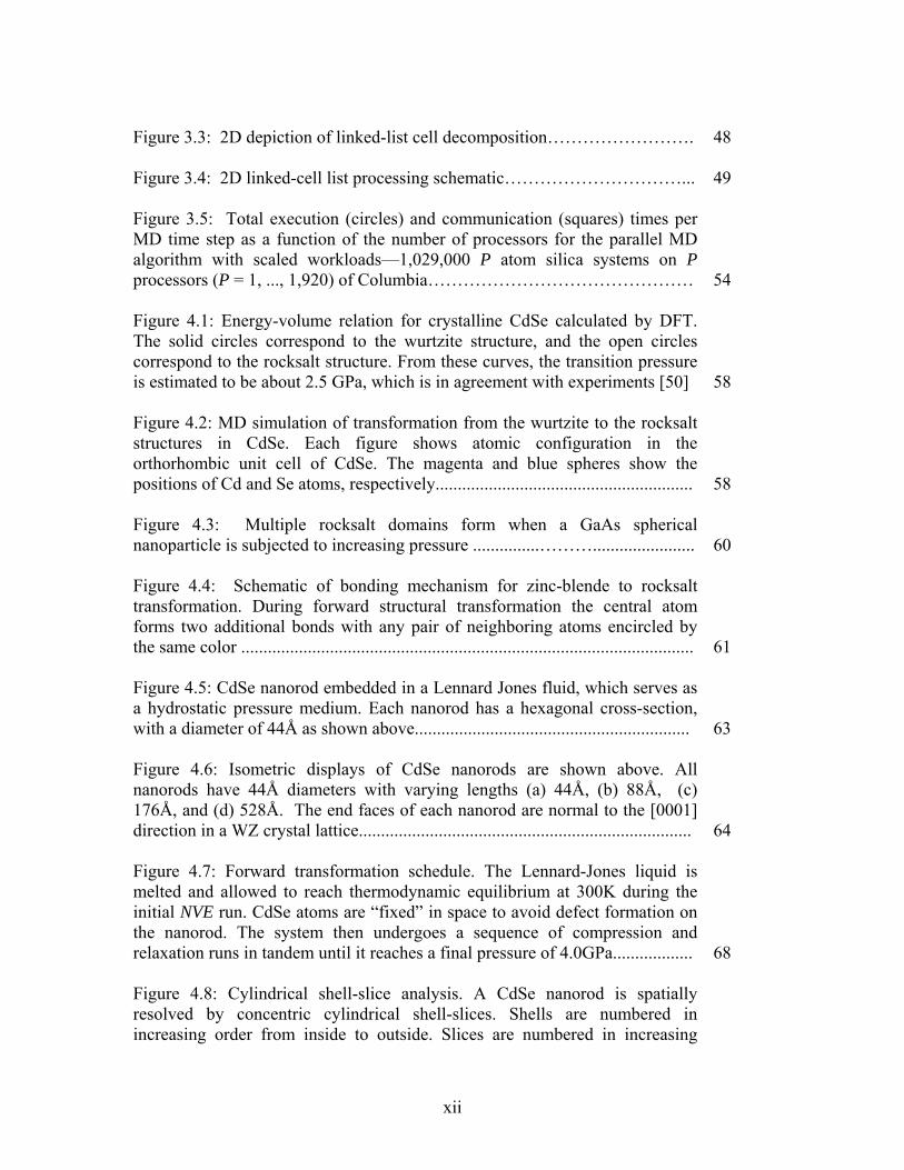
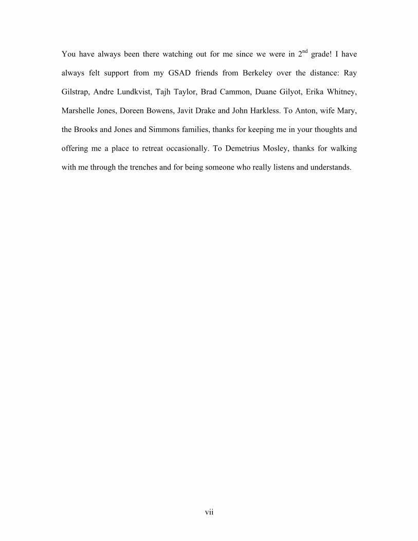
Figure 3.3: 2D depiction of linked-list cell decomposition……………………. 48 Figure 3.4: 2D linked-cell list processing schematic…………………………... 49 Figure 3.5: Total execution (circles) and communication (squares) times per MD time step as a function of the number of processors for the parallel MD algorithm with scaled workloads—1,029,000 P atom silica systems on P processors (P = 1, ..., 1,920) of Columbia………………………………………
54
Figure 4.1: Energy-volume relation for crystalline CdSe calculated by DFT. The solid circles correspond to the wurtzite structure, and the open circles correspond to the rocksalt structure. From these curves, the transition pressure is estimated to be about 2.5 GPa, which is in agreement with experiments [50]
58
Figure 4.2: MD simulation of transformation from the wurtzite to the rocksalt structures in CdSe. Each figure shows atomic configuration in the orthorhombic unit cell of CdSe. The magenta and blue spheres show the positions of Cd and Se atoms, respectively..........................................................
58
Figure 4.3: Multiple rocksalt domains form when a GaAs spherical nanoparticle is subjected to increasing pressure ...............……….......................
60
Figure 4.4: Schematic of bonding mechanism for zinc-blende to rocksalt transformation. During forward structural transformation the central atom forms two additional bonds with any pair of neighboring atoms encircled by the same color ......................................................................................................
61
Figure 4.5: CdSe nanorod embedded in a Lennard Jones fluid, which serves as a hydrostatic pressure medium. Each nanorod has a hexagonal cross-section, with a diameter of 44Å as shown above..............................................................
63
Figure 4.6: Isometric displays of CdSe nanorods are shown above. All nanorods have 44Å diameters with varying lengths (a) 44Å, (b) 88Å, (c) 176Å, and (d) 528Å. The end faces of each nanorod are normal to the [0001] direction in a WZ crystal lattice...........................................................................
64
Figure 4.7: Forward transformation schedule. The Lennard-Jones liquid is melted and allowed to reach thermodynamic equilibrium at 300K during the initial NVE run. CdSe atoms are “fixed” in space to avoid defect formation on the nanorod. The system then undergoes a sequence of compression and relaxation runs in tandem until it reaches a final pressure of 4.0GPa..................
68
Figure 4.8: Cylindrical shell-slice analysis. A CdSe nanorod is spatially resolved by concentric cylindrical shell-slices. Shells are numbered in increasing order from inside to outside. Slices are numbered in increasing
xii

order along the z-axis of the nanorod. A shell-slice is an intersection between a shell and a slice. Structural quantities are calculated for atoms in each shell-slice separately, allowing structural differences between different regions within the nanorod to be monitored and compared during the phase transformation......................................................................................................
70
Figure 4.9: Spatially resolved structural analysis of pristine wurtzite system at T~0K, P~0GPa (NVE). (a) Cd-Cd pair distribution function. (b) Se-Se pair distribution function. (c) Cd-Se pair distribution function. (d) bond-angle distribution. (e) coordination historgram. The curves in each plot are colored red, blue, green, corresponding to the 1st (inner-most), 2nd (middle) and 3rd (outermost) shells, respectively.…......................................................................
71
Figure 4.10: Initial wurtzite structure at T=300K and P=180MPa. Peaks are broadened by thermal fluctuations although.the S1:1 nanorod remains in the wurzite structure..................................………………………….........................
72
Figure 4.11: Intermediate 5-coordinated state at T=300 and P=1.5-2.5GPa. The nanorod begins structural transformation above P=1.0 GPa. Five-coordinated phase, as seen in DFT-MD calculations (Shimojo et al.) is also found here as indicated by the peak at 120º in the bond angle distribution and by five-fold atomic coordination.……………………………………...........................…..…
73
Figure 4.12: Final rock-salt configuration of S1:1 CdSe nanorod at T=300K and P=4.0GPa......................................................................…..................................
74
Figure 4.13 Enthalpy as a function of atomic configuration η. The wurtzite (WZ) and rocksalt (RS) structures correspond to η =0 and 1, respectively. The yellow-open and red-solid symbols show the enthalpy changes calculated along the transformation paths from WZ to RS-I and from WZ to RS-II, respectively. The circles correspond to the paths linearly interpolating the atomic coordinates in the WZ and RS structures. For the lines shown by triangles, the enthalpy of the honeycomb-stacked (HS) structure is shown by η = 0.5.………………………………………………………………………...
76
Figure 4.14: Snapshots of the transformation sequence for the 44Å×44Å CdSe nanorod from MD simulation. Column a) shows the wurtzite-to-rocksalt transformation along [0001] and column b) the corresponding view perpendicular to the z-direction. Rows 1-5 show the nanorod at different pressures..............................................................................................................
78
Figure 4.15: Snapshots of the transformation sequence for the 44Å×88Å CdSe nanorod. The wurtzite-to-rocksalt transformation is shown along the [0001] direction.…………………………………………………………………...........
79
Figure 4.16: Snapshots of the transformation sequence perpendicular to the z-
xiii

direction for the 44Å×88Å CdSe nanorod. Side views of the nanorod at different pressures from 0 GPa to 3.0 GPa are shown here. ................................
80
Figure 4.17: Snapshots of the transformation sequence along [0001] for the S1:4 nanorod..................................................................................................................
81
Figure 4.18: Snapshots of the S1:4 nanorod show the transformation sequence perpendicular to the z-direction at different pressures from 0GPa to 3.5 GPa.……………………………………………………………………...............
82
Figure 4.19: Snapshots of the transformation sequence for the 44Å×528Å CdSe nanorod. Figures a-e show the wurtzite-to-rocksalt transformation along the [0001] direction of the nanorod as the pressure increases to 2.5 GPa............
83
Figure 4.20: Snapshots of the transformation sequence from the 44Å×528Å CdSe nanorod simulation. These snapshots show the wurtzite-to-rocksalt transformation perpendicular to the axis of the nanorod as pressure increases to 2.5 GPa ………………………………………………………………………..
84
Figure 4.21: Snapshots of the nanorod after structural transformation in simulation S1:1. In (a), the top view of the irregular shape of the cross-section after transformations compared with its original hexagonal cross-section outlined in green. A side view of the nanorod, shown in (b), illustrates the extent to which the nanorod contracts along the z-axis........................................
85
Figure 4.22: Top and side views of the nanorod from simulation S1:2 are shown above. The nanorod cross-section becomes irregular and its length along the z-axis contracts during structural transformation. The atoms in the nanorods are arranged in periodic arrays as can be seen from both views, demonstrating that the nanorod is a single rocksalt domain................................................................
86
Figure 4.23: Snapshots from simulation S1:4. A single crystal rocksalt domain forms in the middle of the nanorod. The domain extends out to ~7 atomic layers from the end surfaces where disorder begins due to high-energy surfaces................................................................................................................
86
Figure 4.24: Snapshots of the S1:4, nanorod show that it has become a single rock-salt domain after structural transformation. a) The nanorod has one shape along its shaft from end to end. The end faces remain flat as shown in (b)..........
87
Figure 4.25: Snapshots of the wurtzite-to-rocksalt transformation mechanism. S1:1, nanorod before and after transformation. a) Pristine WZ nanorod at T ~ 0K, P ~ 0GPa b) Transformed nanorod in the RS phase at T = 300K and P = 4GPa. The relative orientation between the initial WZ and final RS lattices indicates WZ to RS-II mechanism...........................................................
87
xiv

Figure 5.1: Brittle material subjected to a stress σ. b) The stress causes cracks in the sample to grow or propagate. The sample suffers cleavage during crack propagation as planes of atoms are peeled apart by crack. c) Brittle fracture results surfaces.......................................................................…………………...
89
Figure 5.2: A sample of ductile material under a tensile stress σ, b) exhibits necking during which the cross-section narrows in one section of the nanorod. c) Necking continues under the influence of the applied stress until the nanorod fractures cross-section of the sample narrows as long as the stress is applied until it disconnects into more than one piece........................................................
90
Figure 5.3: Snapshots of CdSe nanorod cross-sections from simulations (a) S1:1, (b) S1:2, (c) S1:4, (d) S1:12 after structural transformation to a rocksalt phase. The cross-sections of the nanorods change from hexagonal to irregular shapes, while the end faces remain atomically flat in the periodic wurtzite structure...............................................................………………………………..
93
Figure 5.4: Simulation schedule for the reverse transformation………………... 95 Figure 5.5: Final result of 44Å × 44Å reverse transformation, SU-1:1a. a) Snapshot of the nanorod at 180MPa and ~40,000∆t after forward transformation. b) bond-angle distribution, and c) histogram of atomic coordinations.........................................................................................................
96
Figure 5.6: Final result of the 44Å × 44Å reverse transformation, SU-1:1b. The temperature was scaled to stay below 900K. The hexagonal cross-section of the nanorod becomes rectangular. The nanorod is nearly cubic. a) Snapshot of the nanorod at 180 MPa and 500,000 ∆t after forward transformation, b) bond-angle distribution and c) histogram of atomic coordination.................................
97
Figure 5.7: Final results of the 44Å × 88Å reverse transformation. a) Snapshot of the nanorod at 180MPa taken 500,000∆t after forward transformation. b) Bond-angle distribution and c) distribution of atomic coordinations...................
98
Figure 5.8: Final results for the reverse transformation in the 44Å × 176Å nanorod. a) Snapshot of the nanorod taken 500,000∆t after forward transformation at 180MPa. b) Bond-angle distribution and c) histogram of atomic coordinations.............................................................................................
99
Figure 5.9: Three outcomes of the upstroke simulation for the SU1:12 , 44Å×528Å nanorod. The up-stroke simulation begins with the final RS crystal configurations from the preceding down-stroke simulation. Experiments with different temperature-pressure schedules resulted in crystallographic transformation of the nanorod as well as morphological transformations including kinking and fracturing .........................……………………………….
100
xv

Figure 5.10: The sequence of images show necking at several places along the shaft of the 44Å × 528Å nanorod until it disconnects into two pieces. a) Shows the configuration at the end of the forward transformation at 4GPa and 300K. b) Shows the nanorod ∆t later after some amount of decompression at a temperature of ~ 600K and a pressure of 2MPa. c) The nanorod begins to show noticeable necking along the shaft. The necking becomes more pronounced (d) until complete separation takes place (e) ....................................
101
Figure 5.11: A protrusion perpendicular to the axis of the nanorod results during the upstroke after the nanorod temperature increases and is then cooled down.……………………………………………………………………………
102
Figure 5.12: The nanorod kinks at necking points after cooling during reverse transformation…………………………………………………………………...
103
Figure 5.13: Final result for the reverse transformation in SU-1:12 44Å × 528Å nanorod.. a) Bond-angle distribution shows multiple peaks around 90°, 109° and 180°. The nanorod contains both rocksalt and wurtzite crystal phases. b) The histogram of atomic coordination shows amajority of 4-coordinated atoms, which is an indication of the completeness of the reverse transformation...........
104
Figure 5.14: Final results for the reverse transformation in the 44Å × 528Å nanorod. a) Shell-resolved bond distributions show different crystal phases in different shells. The inner-most shell, in red, indicates mixed phases. The blue curve peaks at 109°, which is characteristic of wurtzite and zinc-blende crystal structures. The outer shell represented in green shows a dominant peak at 90°, indicating mostly the rocksalt phase mixed with the wurtzite phase. b) Shows shows 4-coordinated atoms predominating in the atomic coordination histogram ..............................................................................................................
105
Figure 5.15: Peaks at 90° and 180° disappear from all the curves when the atoms at the ends of the nanorod are excluded from shell-resolved bond-angle calculations. Peak at 109.4° in all shells indicates complete reverse transformation to wurtzite begins in the middle of the nanorod and spreads towards the ends. ..........…………………………………………………………
106
Figure 5.16: Snapshots of reverse transformation of 44Å× 528Å CdSe nanorod sliced at different cross-sections from end to end after 251,810∆t. 4, 5, 6-coodinated atoms are colored red, blue and green, respectively. 0-3 coordinated atoms are in gray. The cross-section is virtually all red along the entire core of the nanorod. ...............................................……………………………………...
107
xvi

ABSTRACT
Parallel molecular dynamics (MD) simulations are performed to investigate
pressure-induced solid-to-solid structural phase transformations in cadmium selenide
(CdSe) nanorods. The effects of the size and shape of nanorods on different aspects of
structural phase transformations are studied. Simulations are based on interatomic
potentials validated extensively by experiments. Simulations range from 105 to 106
atoms. These simulations are enabled by highly scalable algorithms executed on
massively parallel Beowulf computing architectures.
Pressure-induced structural transformations are studied using a hydrostatic
pressure medium simulated by atoms interacting via Lennard-Jones potential. Four
single-crystal CdSe nanorods, each 44Å in diameter but varying in length, in the range
between 44Å and 600 Å, are studied independently in two sets of simulations. The first
simulation is the downstroke simulation, where each rod is embedded in the pressure
medium and subjected to increasing pressure during which it undergoes a forward
transformation from a 4-fold coordinated wurtzite (WZ) crystal structure to a 6-fold
coordinated rocksalt (RS) crystal structure. In the second so-called upstroke simulation,
the pressure on the rods is decreased and a reverse transformation from 6-fold RS to a 4-
fold coordinated phase is observed.
The transformation pressure in the forward transformation depends on the
nanorod size, with longer rods transforming at lower pressures close to the bulk
transformation pressure. Spatially-resolved structural analyses, including pair-
distributions, atomic-coordinations and bond-angle distributions, indicate nucleation
begins at the surface of nanorods and spreads inward. The transformation results in a
xvii

single RS domain, in agreement with experiments. The microscopic mechanism for
transformation is observed to be the same as for bulk CdSe. A nanorod size dependency
is also found in reverse structural transformations, with longer nanorods transforming
more readily than smaller ones. Nucleation initiates at the center of the rod and grows
outward.
xviii

CHAPTER 1
INTRODUCTION
Inorganic semiconductors are the foundation of modern electronics. Since the
mid-1950’s, semiconductors have been responsible for a great number of advances in
various technologies including communications, computer hardware and the medical
device industry. They are used in a wide variety of applications among them waste
treatment, air purification, anti-microbial surfaces, chemical and biological
decontamination and solar energy conversion.
Conductive properties of semiconductors make them useful for a wide variety of
technological applications. Semiconductors have special electrical conductivity properties
due to their energy band gap width, which is typically less than 3.5 eV. Compared to
insulators, with energy band gaps generally greater than 5 eV, semiconductor energy
band gaps are small enough for electrons to be excited into the conduction band by
thermal, photonic or other excitations. Introducing dopants or impurities can also alter the
energy band gap of semiconductors and affect their conductivity by orders of magnitude.
Due to this ability to manipulate the conductivity of semiconductors, they are well suited
for the control of key functions of many electronic components including transistors,
diodes, piezoelectric crystal devices and integrated circuits.
Semiconductors are solid state materials found in groups II through VII of the
periodic table. Semiconductors composed of elements from the same group(s) tend to
have similar chemical, electrical and structural properties; which are often studied in
related experiments and employed in similar applications. For example, Si and Ge, group
IV single element semiconductors, are the most commonly used materials in diodes and
1

integrated circuits. This makes them crucial to the electronics industry. Group III-V
semiconductors, like GaN, have large and direct energy-band gaps, which make them
suitable for blue lasers. They are also stable at high temperatures and have good thermal
conductivities, which make them useful in high power transistors. Group II-VI
semiconductors are found in zinc-blende or hexagonal wurtzite crystal structures at 300 K
and have band gaps ranging from 1.4eV to 3.9eV. As these energies correspond to
wavelengths within the visible light range of the electromagnetic spectrum, they have
applications in biological labeling, optoelectronic sensors and photovoltaic devices like
solar cells. Some examples of II-VI semiconductors commonly studied include ZnO,
ZnS, ZnSe, ZnTe, CdS, CdSe, CdTe, HgS, HgSe, and HgTe. This investigation concerns
structural and mechanical properties of CdSe.
It has been shown by that the electrical and optical properties of semiconductors
depend on their structural properties as well as system size. Alivisatos et al. have
performed extensive studies on the synthesis of semiconducting nanocrystals [1], their
optical and electrical properties [2], how these properties change with pressure-induced
structural transitions [3] and their structural stability [4]. Their work includes quantum-
dot assemblies grown on substrates. They have grown nanocrystals of various shapes in
colloidal liquid solutions. Recently, they have conducted experiments on pressure–
induced structural transformations and fracture. Small spherical CdSe nanoparticles, 45Å
in diameter, were observed to undergo reversible, first-order phase transformation,
between 4-coordinated and 6-coordinated states under pressure. Their data indicates the
transformation initiates from a single nucleation event and results in a single domain.
Larger nanocrystals are expected to exhibit dissimilar characteristics approaching those
2

of extended solids―irreversible structural change, multiple nucleation sites and domains,
and bulk fracture behavior.
In the past decade, quantum dot assemblies have been studied experimentally by a
growing number of investigators. Typical quantum dot assemblies are 2-dimensional
arrays of nano-sized islands of semiconducting materials grown on a substrate. Their
special carrier confinement properties enable tunable photo-emission and they emit light
at frequencies that can be controlled by adjusting dot size. This has potential applications
in bioactive fluorescent probes in sensing, imaging, immunoassay, and other diagnostics
applications. Bawendi and co-workers have reported a number of these studies involving
CdSe and ZnS [5, 6].
Colloidal chemistry synthesis is one method by which CdSe nanorods can be
produced without being embedded in substrates and thus has expanded the range of
applications. In this method precursors are dissolved in hot surfactants where they
coalesce to form crystals. Ligand molecules are used to control growth rates of crystals
and the final size of the crystal. Aspect ratio is controlled by surfactant ratio. Rapid
cooling of the surfactant terminates the crystal growth process. The crystals remain
suspended in the mixture.
Alivisatos and co-workers have studied distributions of high-aspect ratio nanorods
to examine multiple domain characteristics and irreversible structural transformation. X-
ray diffraction pattern analysis reveals that multi-domain behavior increases with the
aspect ratio (length-to-width) of nanorods. They sought a critical length scale governing
fracture behavior and proposed a mechanism by which fracture might occur in CdSe
nanorod ensembles. Observations of changes in diffraction line widths during pressure
3

cycling appear to support the proposed mechanisms of transformation. Diffraction peak
widths are inversely proportional to crystallite size. Line widths for small nanocrystals
remain the same through an indefinite number of cycles. Line widths of nanocrystals with
higher aspect ratios broaden as expected after the first pressure cycle and then remain
constant for subsequent cycles, indicating that longer nanorods into smaller ones. CdSe
nanorods have been shown to undergo multiple fractures during phase transformation
under compression. Evidence of longer nanorods fracturing into shorter ones under
compression can be seen in the transmission electron microscopy images shown in Figure
1.1. Figure 1.2 shows that the average length of the nanocrystals after compression is less
than half the initial length, indicating that the nanorods tend to fracture into more than
two pieces.
A B
Figure 1.1 Transmission electron micrograph of representative CdSe nanorods in the 4-coordinate phase before (A) and after one (B) pressure cycle.
A timescale for phase transformations is estimated from kinetics of
transformations under abrupt pressure changes. Ensembles of CdSe nanorods were
demonstrated to transform on the order of seconds to hours in Alivisatos’ experiment.
4

However, it is thought that the time required for an individual nanocrystal within an
ensemble to structurally transform could typically be on the order of picoseconds.
Figure 1.2 Length distribution of the particles before (blue) and after (red) pressure cycling.
The mechanism of transformation is believed to be an event where the planes
slide sequentially in a direction perpendicular to the shaft of the rod. It is thought that this
progresses uniformly throughout the nanocrystal from the slanted shapes of the rods that
result after sliding of planes. The CdSe rods studied in these experiments have zinc-
blende or faulted wurtzite crystal structures. It would be interesting to see if this
mechanism also occurs in mono-crystalline wurtzite CdSe rods.
Turning to computer simulation, advances over the years in algorithms and
computing hardware have led to the development of a powerful tool. Simulation is now a
well-established mode of research; an intermediate between theory and experiment that
provides perspectives inaccessible to both.
Simulation can be applied towards a wide range of systems: mechanical devices,
ecological problems, meteorological studies, economics, control and operation research
5

processes, fluid flow, and robotics. Special algorithms have allowed simulations to keep
pace with accelerating advances in hardware as envisioned by Gordon Moore, having a
synergistic effect on the development of high-performance computing. System sizes of
atomistic simulations have also grown at an impressive rate. By 2010, it is expected that
large-scale computers will perform simulations within the petaflop regime, involving
more than 10 billion atoms, and allowing atomistic analysis of physical system which
exceeding 1 cubic micron in size.
Gordon Moore observed in 1965 that the number of transistors per square area on
integrated circuits had doubled every year since the integrated circuit was invented.
Moore predicted that integrated circuit complexity would continue to increase at this rate
over the years leading into the 21st century. Since then, computer memory and
microprocessor technology have generally followed his projection as data density and
processor speeds have doubled approximately every 18 months. This trend, now
commonly known as Moore’s law, is expected by most experts to hold for at least another
two decades. Figure 1.3 charts how attainable system sizes for simulations have grown
with the ongoing developments in algorithm and hardware design since the time of
Moore’s prediction.
A number of the groups in the computational science are following this
computing evolution from teraflops (1012 flops) to petaflops (1015 flops). Using this
unprecedented computing power, these groups will be able to carry out realistic
simulations of complex systems and processes in the areas of materials, nanotechnology,
and bioengineered systems. Coupled with immersive and interactive visualization, this
6

will offer unprecedented opportunities for research as well as improving graduate and
undergraduate education in science and engineering disciplines.
Figure 1.3 Simulated system sizes in the framework of density functional theory (DFT) and molecular dynamics (MD) have kept pace with Moore’s Law due to advances in algorithms and hardware.
Recent computer simulation studies have contributed significantly to our
understanding of nanosystems in the case of semiconducting nanoparticles. Numerical
experiments have paralleled experimental work in the exploration of CdSe
semiconducting nanoparticles. Molecular Dynamics (MD) and Density Functional
Theory (DFT) calculations have been performed to investigate structural phase
transformation under pressure. Calculations based on DFT by Shimojo and others [7],
reveal that several possible transformation paths between CdSe’s characteristic wurtzite
phase and high-pressure rocksalt phase. However, DFT system sizes are typically limited
to only a few hundred atoms. Finite-size effects may result in different mechanical
behavior in bulk than in such small systems. MD simulations of structural
transformations in CdSe nanoforms, such as the rods we present in this work may
increase understanding of physical properties of CdSe for larger system sizes.
7

MD simulations make it possible to study nanocrystals under ideal conditions and
to compare them with experimental systems, which may have defects. This can help in
isolating competing factors contributing to a certain phenomenon. For example, micro-
defects affect fracture in nanomaterials, and these can be precisely specified and tested by
MD simulations. This level of control over micro-defects does not exist in experiment.
Conventional MD simulations are performed in the microcanonical ensemble
where the number of atoms the total volume and energy of the system are held constant.
However, many actual experiments involve the study of physical systems under constant
pressure and/or temperature, where either volume or total internal energy fluctuates.
These ensembles require extension of conventional MD method to the canonical (NVT)
or isobaric-isothermal ensemble (NPT).
A number of methods for NVT MD have been proposed through the years
beginning in the early 1980’s when Andersen proposed a stochastic procedure to sample
random velocities from a Maxwell-Boltzmann distribution and assigning them to
particles based on a specified particle collision rate [8]. However, limitations in this
method were found when Tanaka et al. applied Anderson’s method to water and Lennard-
Jones systems [9]. An undesirable coupling between the system’s temperature and its
diffusion coefficient was found to exist above a certain stochastic collision probability
threshold. Hoover introduced a method constraining a system’s kinetic energy through a
velocity dependent term in the potential [10]. Although the method generates a canonical
ensemble, it imposes an unphysical suppression of kinetic energy fluctuations.
In 1983, Nosé (who unfortunately passed away recently at age 54) proposed a
molecular dynamics method for simulations in the canonical ensemble [11]. It maintains
8

constant temperature in the system by introducing an additional variable, s, giving an N-
atom system 3N+1 degrees of freedom. The variable s couples to the kinetic energy of
the system and thus links the physical system to a heat bath, with which energy can be
exchanged to regulate temperature. Nosé’s method does not suffer from the limitations of
the NVT methods previously described. His method is purely dynamical, involving
deterministic, reversible equations of motion as opposed to stochastic methods and
generates averaged physical quantities belonging to the canonical ensemble.
In the late 1970’s, Anderson presented a constant enthalpy and constant pressure
(NPH) MD technique [12]. His method involves an MD cell having variable volume
determined by a balance between the internal pressure of the system and the external
pressure. The method conserves enthalpy and maintains constant pressure. Parinello and
Rahman later extended this method to incorporate a parallelepiped MD cell, capable of
changing shape and volume in time [13]. This method maintains constant stress σ. Three
time-dependent vectors c ,b ,a rrr and define the edges of the MD cell and the number of
degrees of freedom of an N-atom system increase from 3N to 3N + 9. Parinello-Rahman
formulation leads to a modified Lagrangian where the atomic velocities in the kinetic
energy are transformed in relation to the varying MD cell dimensions. Two additional
terms also appear in the Lagrangian; one is a kinetic-energy-like term which taken into
account the kinetic energy of the MD cell, and the other is, associated with the elastic
energy of the MD cell due to the external stress on the system. This extended MD method
allows the study of solid-to-solid structural transformations and other constant pressure
calculations.
9

Nosé’s method for NVT simulation can be combined with the HPN simulation to
generate NPT ensembles. The NVT and NPT MD simulations for this thesis are
implementations of the methods proposed by Nosé and Parinello-Rahman. These
methods will be further described in Chapter 2.
MD experiments have been used to simulate pressure-induced structural
transformations in GaAs semiconductor nanocrystals to characterize deformation and
grain formations [14]. These studies were motivated and guided by earlier ab initio
simulations in bulk SiC and GaAs where new structural transformation mechanisms were
identified [15][16]. The initial configuration of the simulation, shown in Figure 1.4,
consisted of a 30 Å-radius single crystal nanoparticle of ~5000 GaAs atoms, positioned at
the center of a 123 Å cubic MD cell surrounded by a distribution of ~500,000 atoms
representing a fluid medium. The fluid medium was simulated by a distribution of atoms
interacting via Lennard-Jones potential, and provided a means to apply hydrostatic
pressure to the nanoparticle. The atoms of the GaAs nanoparticle interacted through a
potential developed by Vashishta et al.
Figure 1.4 Initial simulation setup for a GaAs spherical nanoparticle surrounded by a distribution of atoms interacting via Lennard-Jones potential.
10

Initially, the system was allowed to reach thermal equilibrium at 2.5 GPa.
Pressure in the system was then increased in increments of 0.5 GPa per 10000 time-steps
until the system pressure reached 22.5 GPa. The onset of structural transformation of the
nanoparticle from 4-coordinated, zinc-blende, to 6-coordinated, rocksalt, was observed at
pressures approaching 16.2 GPa. The total transformation occurred at a pressure of 22.5
GPa.
A shell-resolved analysis of the nanoparticle during structural transformation
showed nucleation at the surface of the nanoparticle spreads inward to the center of the
nanoparticle. Figures 1.5 (A) and (C) show configurations of the GaAs nanoparticle at
17.5 GPa and 22.5 GPa, just before transformation. All shells are concentric about the
geometric center of the nanoparticle and numbered from innermost to outermost as
indicated by the yellow circles. Plots of corresponding bond-angle distributions for each
shell are displayed in Figures 1.5 (B) and (D). In Figure 1.5 B, curve 1, the red peak
centered about 109.4º indicates that the core of the nanoparticle remains in the
characteristic zinc-blende crystal form at 17.5 GPa while the surrounding shells bond
angle distribution, indicated in green, shows a shift towards 90º. The outermost shell
contains 6-coordinated atoms in the rocksalt structure, as indicated by the blue curve with
peaks at 90º and 180º. Figure 1.5 D shows pronounced peaks at 90º and 180º in all three
curves, indicating a complete structural transformation from 4-coordinated zinc-blende to
6-coordinated rocksalt structure. The final configuration of the GaAs nanoparticle reflects
the rocksalt phase with multiple domains having different orientations. This is an
indication of multiple nucleations. However, experiments show that multiple nucleation
11

events are rare in small nanoparticles because they are mostly found as single crystals.
This aspect of structural transformation will be discussed further in Chapter 4.
Electronic structure calculations based on DFT were performed on bulk CdSe
systems by Shimojo et al. Isothermal-isobaric MD calculations were carried out on bulk
CdSe to identify transformation paths. In the initial setup, the temperature of the system
was 300 K and the pressure 0.5 GPa. The pressure of the system was then increased in
increments of 1 GPa per 1000 time steps (1 time step = 2 fs). Next, the system was
allowed to relax for 5000 time steps. This sequence of pressure “ramping” and
“relaxation” was repeated until the pressure on the system reached 6 GPa. Energy vs.
volume relations for the bulk CdSe in wurtzite and rocksalt phases were obtained from
the DFT calculations. The transition was observed at 2.5 GPa. DFT calculations showed
two Fm3m crystallographic, rocksalt structures as being energetically favorable at 2.5
GPa. The two rocksalt structures RS-I and RS-II, are reached from different and have
different crystal orientations. A metastable five coordinated state, P63/mmc
crystallographic structure, was also observed between the 4-fold and 6-fold coordinated
states. These results and structural transformations in CdSe spheres and rod-shaped
nanoparticles will be discussed in depth in Chapter 4 and compared with ab-initio
calculations.
The outline of the remaining portion of this dissertation is as follows. Chapter 2
contains further descriptions of extended molecular dynamics methods and
implementations of molecular dynamics on parallel computing systems are presented in
Chapter 3. Results of simulations and comparisons with experiments on pressure-
induced structural transformations in CdSe nanoparticles will be discussed in Chapter 4.
12

Chapter 5 will focus on high-aspect-ratio CdSe nanorods and include additional
descriptions of multidomain formation and fracture. Conclusions are presented in Chapter
6.
A B
C D
Figure 1.5 Molecular dynamics configurations of GaAs nanoparticles at pressures of (A) 17.5 GPa and (C) 22.5 GPa. Corresponding spherical shell-resolved bond angle distributions are shown in figures B and D, respectively.
13

CHAPTER 2
MOLECULAR DYNAMICS METHODOLOGIES
In this chapter we discuss molecular dynamics (MD) methodology in various
ensembles and numerical calculations of structural, thermomechanical and dynamical
quantities.
2.1 Background
Molecular dynamics (MD) involves numerical solution of Newton’s equation for
a system of atoms interacting via a specific interatomic potential†.
VFrm iiii −∇==r
&&r 2.1
where is the interatomic potential, V irr is the position of atom i, and is the force
exerted on atom i by other atoms, and
iFr
2
2
dtrd
r ii
r&&r = .
The system of 3N second-order ordinary differential equations can be solved
numerically using finite-difference methods. Given an initial set of positions and
momenta { (0), (0)} for all the particles, the equations of motion are discretized using
a small time step, ∆t, and propagated forward in time {
irr
ipr
irr (t), (t)}→{ (t+∆t),
(t+∆t)}…. This will be discussed in more detail in section 2.1.3.
ipr irr
ipr
† The average DeBroglie wavelength, λ, for a system in equilibrium at a temperature T is given as Tmkh B2/=λ . Let a be the average distance between two atoms in a system. The classical approximation holds whenever a>>λ. Thus whenever the average spacing between atoms is greater than the DeBroglie wavelength, quantum mechanical effects, although ever present in the system, are insignificant and can be ignored. At 300K, λ = 0.15Å. At the highest number density reached in our simulations is 0.26 1/Å3 at which a ≈3 Å.
14

In addition to initial conditions, it is also necessary to specify appropriate
boundary conditions (PBC). For example, for bulk systems periodic boundaries are
applied by replicating the MD cell with all its atoms in all directions. The positions and
velocities of the atoms in the replicated systems are identical to those in the original MD
cell. An atom interacts with other atoms inside the MD cell and with the images of atoms
in the replicated systems within the cut-off range of the potential. This is known as the
minimum image convention. If an atom leaves the MD cell, its image enters the cell from
the opposite face. Figure 2.1 is an illustration of periodic boundary conditions applied to
a two-dimensional system.
PBC minimizes surface effects in a well-defined manner. However, there are
caveats in using PBC. Properties that depend on long-wavelength contributions, e.g. the
static structure factor for small wave vectors, are limited by the size of the MD cell and
affect comparison with experiments.
Figure 2.1 A two-dimensional illustration of periodic boundary conditions. An MD cell containing atoms is shown in blue. Replicas containing atom images are in white. Interactions between atoms and image atoms are indicated by the black lines connecting them. When an atom moves across a boundary on one side of the box, its image enters through the opposite side.
Initial conditions are assigned to positions, irr and momenta, , of particles.
Initial atomic positions depend on the type of system, its current state and the objective of
ipr
15

the simulation or run. Usually, for crystalline systems, the atoms are placed at their
equilibrium lattice positions and assigned random velocities chosen from a Gaussian
distribution. The number of atoms and the size of the MD cell are chosen to have the
correct density. An amorphous system is prepared by melting a crystalline system and
quenching the molten state.
Atomic forces and potential energy can be calculated efficiently using the linked-
list method. A linked list is a data structure made up of an unbroken chain of elements,
where each element consists of two parts― one part containing data and the other a
reference, or link, to another element in the structure as shown below.
Figure 2.2: An illustration of a singly connected link list. The solid circle at the end represents the null element, which contains no data and simply terminates the list.
The linked-list exploits the idea that forces between atoms beyond a certain cut-
off radius, rc, are negligible. In calculating the force on a particular atom, excluding
atoms beyond a certain cut-off radius, rc, significantly reduces the amount of computing
time while maintaining a reasonable approximation for the total force.
In the implementation of the linked-cell list scheme, all atoms in the MD cell are
spatially sub-divided into smaller cells. A linked-cell list is organized for each cell to
contain all data pertaining to each atom within that cell. Force calculations are performed
for each atom, i, with all its “neighboring” atoms, j, in the same linked-cell list. Force
calculations are also performed between atoms across adjacent and diagonal cells within
the cut-off range rc. Since atoms may move between cells, linked-cell-neighbor lists must
be reconstructed each time atomic coordinates are updated.
16

rc
Figure 2.3: Illustration of link-cell neighbor list scheme: The center cell (in dark blue) represents any sub-cell of the subdivided MD system. In this instance, interactions between all atoms in the dark blue cell are computed along with interactions with atoms in neighboring cells (indicated in light blue) within the cut-off range rc. Interactions with non-neighboring cells (not shaded) are not included in the force sum for atoms in the dark blue cell. This greatly increases the efficiency of MD computations.
A brute-force algorithm, one that would compute the sum of forces on all possible
pair combinations of atoms in the MD cell, would have a computational complexity of
O(N2), where N is the number of particles. Linked-cell-neighbor lists reduces this
complexity to O(N). The advantage of linked-cell list over brute force computing
increases with the size of the system.
2.1.1 Interatomic Potentials
The interatomic potential function is the most essential input to any MD
simulation, since it determines the realism of a simulation. Over the years, a number of
potentials have been developed for various materials including the embedded atom
17

potential [17], the shell model [18], bond-order potentials, etc. [19]. The interatomic
potential is usually taken to be a sum of one-body, two-body, three-body…contributions.
∑∑∑≠<<
+++=ikj
kjiji
jii
iN rrrVrrVrVrrV ...),,(),()(),...,( )3()2()1(1
rrrrrrrr
2.2
The first term represents interactions of particles with an external field. The
second term is a 2-body potential, which incorporates the interaction between atomic
pairs. Typical 2-body potentials are the Lennard-Jones (LJ) interaction for systems of
inert gas atoms or the Coulomb potential for systems containing charged particles. The LJ
interaction was used in our simulations to represent a liquid hydrostatic pressure medium.
The functional form of the LJ potential is,
⎥⎥
⎦
⎤
⎢⎢
⎣
⎡
⎟⎟⎠
⎞⎜⎜⎝
⎛−⎟
⎟⎠
⎞⎜⎜⎝
⎛=
612
4)(ijij
ij rrrV σσεr
2.3
Here, ε , is the potential well depth and σ is the length parameter of the potential.
Three-body terms are important for semiconductors. The Stillinger-Weber
potential is an example of a 3-body potential and has the general form:
( )2)3( coscos)()()cos,,( jikjikikikijijjikjikikij rfrfBrrVjik
θθθ −= 2.4
where f(r) is a decaying function with a cutoff between the first- and the second-neighbor
shells and jikθ is the angle between the ijrr and ikrr bonds,
ikij
ikijjik rr
rr rr⋅
=θcos 2.5
The basic idea of Stillinger-Weber potential is that it imposes a penalty function so that
the angles are close to the prescribed value jikθ which reflects the structure of the system.
For example, in a tetrahedrally coordinated system, the angle jikθ within each
18

tetrahendron is 109.4º. Deviations from this angle raise the energy of the system. is
the strength of the interaction. 4-body terms have been used in simulations of polymer
chains in SAMs [20] and some metallic systems [see the work by Moriarity at
Livermore]. Multi-particle potentials higher than four bodies are not common.
jikB
There are also interatomic potentials in which certain parameters vary depending
on the local environment of an atom. An example of these potentials is the so-called
bond-order potentials. The Tersoff potential is one such potential, generally expressed as:
[ ]∑ −=ji
ijAijijR rVbrVV,
)()(21 2.6
)( ijA rV is an attractive term arising from the bonding of valance electrons and
is a repulsive term that takes into account steric effects. One feature found in
metals and semi-conductors is that cohesive energy decreases with coordination. The
parameter captures this feature, as it decreases with increasing atomic coordination.
Bond-order potentials work well for a variety of materials. However, the drawbacks are
that such potentials are short ranged and do not incorporate charge transfer which
restricts the range of application to materials with covalent bonding. Recently, Goddard
and co-workers have incorporated charge-transfer effects in bond-order potentials.
)( ijR rV
ijb
The potential used in our MD simulations of CdSe was developed by Vashishta et
al. It consists of two-body and three-body interactions and has the following functional
form:
∑∑≠<<
+=ikj
kjiji
jiN rrrVrrVrrV ),,(),,(),...,( )3()2(1
rrrrrrr
2.7
where
19

6/
4/2 41
ij
ijrr
ij
ijrr
ij
ji
ij
ijij r
We
rD
erZZ
r
HV sijsij
ij+++= −−
η
2.8
2
23
)cos(cos1)cos(cos
00
jikjik
jikjikrrrrjikijk C
eBV ikij
θθθθγγ
−+
−= −
+−
2.9
and
)(21
)(
22ijjiij
jiijij
ZZD
AH ij
αα
σσ η
+=
+=
2.10
Two-body terms represent steric repulsion, screened Coulomb, charge-dipole, and
van der Waals interactions. The three-body terms represent bond bending and stretching.
The parameters in this potential were fitted to reproduce experimental values for
CdSe, including lattice constant, cohesive energy, and elastic constants for the crystalline
phase. The potential gives a good description of melting temperature, fracture energy,
and phonon density of states. The potential also gives good agreement with experimental
X-ray static structure factor of amorphous CsSe. Additionally, a high-pressure phase
transition from wurtzite (4-fold coordination) to rocksalt (6-fold coordination) is also
correctly described. The values for the potential parameters used are given in Table 2.1.
Table 2.1. Parameters for Cd-Se Interaction
Parameter Value
ACd-Cd 3.7576×10⁻¹⁹ J ASe-Se 0.9394×10⁻¹⁹ J ACd-Se 0.9394×10⁻¹⁹ J σCd 1.1 Å σSe 1.54 Å
ηCd-Cd 7 ηSe-Se 7 ηCd-Se 9 ZCd 1.0438 e
(table continued)
20

ZSe -1.0438 e αCd 0.0 Å3
αSe 5.0 Å3 WCd-Cd 0.0 J Å6 WSe-Se 0.0 J Å6 WCd-Se 11.9135×10⁻¹⁸ J Å6
r1 5.0 Å r4 2.5 Å
Bijk 1.5×10⁻¹⁹ J γ 1.0 Å r0 3.8 Å ijkθ 109.4712°
2.1.2 Force Calculations
The most compute-intensive part of a molecular dynamics simulation is the
calculation of atomic forces, potential energy, atomic-level stresses, etc. Brute force
calculation of pairwise interactions between N involves O(N2) operations. This
computational complexity can be reduced to O(N) for short ranged forces using linked-
cell list techniques which will be discussed later in Chapter 3. For long-ranged forces the
fast multipole method by Greengard and Rokhlin [21] can reduce the complexity to O(N).
2.1.3 Integration Algorithms
The Gear predictor-corrector algorithm is one of the early finite difference
methods used to find solutions to ordinary differential equations. This method was and
still is commonly used to solve the equations of motion in MD. The basic idea can be
described in 3 steps.
1. Predictor-step: Taylor expansions of positions and their time derivatives up to a
desired order are calculated to obtain approximate values for position, velocity and
acceleration, etc.
21

)(...)()(
)(...)()()(
)(...)()2/1()()()(
)(...)()6/1()()2/1()()()(2
32
qp
qp
qp
qp
tOtbttb
tOttbtatta
tOttbttatvttv
tOttbttattvtrttr
++=∆+
++∆+=∆+
++∆+∆+=∆+
+++∆+∆+=∆+
rr
rrr
rrrr
rrrrr
2.11
2. Force evaluation- Atomic forces and accelerations are calculated from the gradients of
the potential energy. Since the actual acceleration is different from predicted values in
step 1, the error must be corrected. This is done in the correct-step.
)()()( ttattatta pc ∆+−∆+=∆+∆rrr 2.12
3. Corrector-step- Predicated values of accelerations are calculated as follows:
)()()(
)()()()()()(
)()()(
3
2
1
0
ttacttbttb
ttacttattattacttvttv
ttacttrttr
pc
pc
pc
pc
∆+∆+∆+=∆+
∆+∆+∆+=∆+
∆+∆+∆+=∆+
∆+∆+∆+=∆+
rrr
rrr
rrr
rrr
2.13
The values of coefficients c0, c1, c2, and c3 depend on the order of the differential
equation being solved. These coefficients have been tabulated by Gear for various
differential equations [22,23]. The Gear predictor-corrector algorithm can be run multiple
times to achieve better accuracy. However, one should be mindful that the corrector step
requires force calculations, which are computationally expensive. So one should gauge
how much iteration is necessary at each time step.
The most commonly used integration algorithm in MD is the Verlet algorithm,
which is expressed as:
)()()()(2)( 42 tOttattrtrttr +∆+∆−−=∆+rrrr 2.14
It is obtained by adding.
22

)()()6/1()()2/1()()()(
)()()6/1()()2/1()()()(432
432
tOttbttattvtrttr
tOttbttattvtrttr
+∆−∆+∆−=∆−
+∆+∆+∆+=∆+rrrrr
rrrrr
2.15
The Verlet formulation is stable and relatively easy to implement. As can be seen,
the truncation error is 4th order. Velocities can be calculated from the positions,
tttrttrtv
∆∆−−∆+
=2
)()()( . 2.16
One of the most stable algorithms is a variant of the Verlet algorithm and is called the
velocity-Verlet algorithm. Here,
)()(21)()()( 32 tOttattvtrttr +∆+∆+=∆+
rrrr . 2.17
From the positions at time , the forces and accelerations are computed at .
Subsequently, the velocity at time
tt ∆+ tt ∆+
tt ∆+ is calculated from,
tttattvttv
ttrVm
tta
∆∆++∆
+=∆+
∆+∇−=∆+
)(21)
2()(
))((1)(
rrr
rr
2.18
The velocity-Verlet algorithm is used in all the simulations reported here. The
algorithm conserves the total energy very well in the microcanonical algorithm.
A time integration algorithm should conserve the phase-space volume. Velocity-
Verlet algorithm preserves phase space and is time-reversible [24]. Tuckerman et al. have
demonstrated time reversibility and phase-space volume conservation from the Liouville
formulation of classical mechanics. The Liouville operator is defined as:
∑ ⎥⎦
⎤⎢⎣
⎡∂∂
+∂∂
=i i
ii
i pf
qviL r
rr
r 2.19
23
where fr
is the force acting on the ith particle. Let },{ ii pq rr=Γ represent the instantaneous
state of the system in the phase space. The classical propagator is then
Then the state of the system, , can be propagated as follows:
tiLetU ∆=∆ )( .
Γ
)0()()0()( Γ=Γ=Γ tUet iLt 2.20
[Note: is a unitary operator, i.e. time reversible: ]. The Liouville
operator can be split into two parts.
)(tU )()( 1 tUtU −=−
21 iLiLiL += 2.21
where
∑∑ ∂∂
=∂∂
=i i
ii i
i pfiL
qqiL r&rr& 21 , 2.22
)()( 3121 tOeeeetU tiLtiLtiLtiL ∆+==∆ ∆∆∆∆ 2.23
We can obtain the state of the system, Γ , at a time tt ∆= by applying the as )( tU ∆
∑∂∂∆
∑∂∂
∆∑∂∂∆
=∆
∆∆
=∆ i ii
i ii
i ii p
vtp
ftq
vt
eeetUtUtUtUr
rr
rr
r
22121 )
2()()
2()( 2.24
The system is propagated to a state )( tn∆Γ by successively applying the operator )( tU ∆
n times. Operating with this factorization on )}0(),0({ ii pq rr=Γ and using the identity,
)()( txfxfe xt
+=∂∂
, 2.25
for the positions and velocities at time t∆ are obtained as
)0(2
)()0()0()(2
iiii pmtp
mtqtq
r&
rrr ∆+
∆+=∆ 2.26
[ ])()0(2
)0()( tpptptp iiii ∆+∆
+=∆r&
r&
rr 2.27
which are identical to the equations of the velocity-Verlet algorithm.
24

2.2 Statistical Ensembles
Statistical mechanics is the basis of MD methodology. In statistical mechanics,
macroscopic or thermodynamic quantities are calculated from ensemble averages over all
possible thermodynamically identical states of the system. Correspondingly, in MD,
macroscopic quantities are computed from time averages of microscopic
states, , expressed in terms of atomic positions, ))(),(( tptr iirr
Γ irr and momenta, , where
i = 1,…,N, for a system of N atoms. Each microscopic state, Γ, can be considered a point
in a multidimensional D×N space where D is the number of spatial dimensions. An
ensemble in MD is a collection of microscopically distinct states in the 6N-dimensional
phase space, Γj. Here, we will discuss the microcanonical, canonical, and isobaric-
isothermal ensembles.
ipr
Microcanonical ensemble describes systems in thermodynamic states expressed
by constant variables N, V, E which denote fixed number of particles, volume, and energy
respectively. In the NVE ensemble, the Hamiltonian and equations of motion are
∑=
+=N
ii
i
i rVmpH
1
2
})({2
r
2.28
ii
ii r
HppHr r
r&r
r&
∂∂
−=∂∂
= , 2.29
2.2.1 NVT Ensemble
Extended MD methods are used for other ensembles. In the canonical ensemble,
temperature is fixed and energy is allowed to fluctuate. This requires adding a term that
acts like a heat bath to exchange energy with the system. NVT-MD, first proposed by
25

Nosé, prescribes a Hamiltonian, which includes a thermostat variable s to regulate
constant temperature.
The thermostat has an associated mass, Q, and momenta ps. The Hamiltonian for
NVT MD is,
∑ ++++=N
ireqB
si
i
iext sTkf
Qpr
smpH )ln()1(
2})({
2
2
2
2 rφ 2.30
where is the number of degrees of freedom, is Boltzmann’s constant, and T is the
temperature to be maintained in the system by the heat bath. The equations of motion are,
f Bk
∑ +−=
−=∆
ireqBi sTkfsmqsQ
sqsmsftq
/)1(
/2/)(
2
2
&&
r&&
rr&&
2.31
The logarithmic dependence of the variable, , in the Hamiltonian, is essential in
producing the canonical ensemble [25]. The equations of motion for this Hamiltonian are
written in virtual variables which are related to the real variables
s
tpq ii ,, rr tpq ii ′′′ ,, rr as,
,ii qq rr=′ 2.32
,/ spp iirr
=′ 2.33
,∫=′sdtt 2.34
and the real velocity is expressed in scaled form as,
dtqds
dt
qd iirr
=′
′
2.35
Nosé-Hoover chains address the problem of non-ergodicity by “linking”
additional thermostats si to the system. All thermostats, si, are coupled. That is, energy
26

can be exchanged between any thermostat, si and any other thermostat, sj. Coupling
between thermostat variables drives fluctuations in ps, effectively filling the phase space.
The method preserves the advantages and simplicity of the original approach. The
Hamiltonian for an MD system with Nosé-Hoover chains is,
∑ ∑∑= ==
++++=N
i
M
iireqBreqBf
M
i ii
i
i TkTkNQ
pr
mpH i
1 21
1
22
2})({
2ξξφ ξr
2.36
where the additional degree of freedom s is related to the variable
11log ξfNs = 2.37
iis ξ=log 2.38
Thermostat masses, , are determined from, pQ2/
1 preqBfp TkNQ ω= 2.39 2/ preqBpi TkQ ω= 2.40
where pω is the natural frequency of the heat bath.
Martyna et al. have implemented explicit reverse integrators for the Liouville
operator using the Trotter formula [26]. The Liouville operator for the Nosé-Hoover
chain of M thermostats coupled to an N particle system is expressed as,
MM
i
M
ii
M
i iv
N
iiv
N
i i
ir
N
ii GGv
mrFviL
iiiiiiξξ
ξξξξ νννν
ξνν
∂∂
+∂
∂−+
∂∂
+∇⋅−∇⋅⎥⎦
⎤⎢⎣
⎡+∇⋅=
+∑∑∑∑∑−
=====
)()(11
1
11111
rrrrrrr 2.41
where are given by, sG'
⎟⎠
⎞⎜⎝
⎛−= ∑
=
N
ireqBfi TkNvm
QG
i1
2
11
1,
2.42
( )reqBii
i TkvQQ
Gi
−= −−2
111
ξ , 1>i2.43
The Trotter formula can be generalized to express the evolution operator as,
27

)( 32222 12
1 tOeeeeeetiLtiLtiL
tiLtiLtiL NHCNHC∆+=
∆∆∆
∆∆∆ 2.44
where and are defined as 1iL 2iL NHCiL
i
i
r
N
ii
v
N
i i
i
viL
mrFiL
∇⋅=
∇⋅⎥⎦
⎤⎢⎣
⎡=
∑
∑
=
=
rr
rr
12
11
)(
2.45
and
MM
i
M
ii
M
i iv
N
iiNHC GGviL
iiiiξξ
ξξξξ νννν
ξνν
∂∂
+∂
∂−+
∂∂
+∇⋅−=+∑∑∑
−
===
)(11
1
111
rr 2.46
Substituting and into the generalized Trotter formula for the time-evolution
operator yields the full-time evolution. The Nosé-Hoover chain part of the evolution
operator,
1iL 2iL NHCiL
2tiLNHCe
∆
, is expressed as:
∏=
∆∆
=c
cNHCNHC
n
i
ntiLtiL
ee1
22 2.47
where a multiple time step approach has been used. The operator ),1( >cn 2tiLNHCe
∆
is first
applied to update the { }vv rr ,, ξξ variables. Next the updated velocities are used as input to
the velocity-Verlet step, ⎟⎟⎠
⎞⎜⎜⎝
⎛ ∆∆
∆22 1
21
tiLtiLtiL
eee , and finally the last 2tiLNHCe
∆
is applied to the
output of the velocity-Verlet step. This procedure is summarized as follows:
⎥⎦
⎤⎢⎣
⎡⎟⎠⎞
⎜⎝⎛ ∆
∆=∆2
),0(;)( tvrtrtr Vrrrr
ν 2.48
⎥⎦
⎤⎢⎣
⎡⎟⎠⎞
⎜⎝⎛ ∆
∆′∆=∆
2),(;
2)( tvtvtvtv NHC ξ
rrrr 2.49
⎥⎦
⎤⎢⎣
⎡⎟⎠⎞
⎜⎝⎛ ∆
∆′∆∆=∆
2),(),
2(;
2)( tvtvttt NHC ξξξξ rr
2.50
⎥⎦
⎤⎢⎣
⎡⎟⎠⎞
⎜⎝⎛ ∆
∆′∆=∆
2),(;
2)( tvtvtvtv
NHC ξξξrrrr 2.51
where
28

( )⎥⎦⎤
⎢⎣⎡∆
=⎟⎠⎞
⎜⎝⎛ ∆ 0),0(;
22 ξvvtvtvNHC
rrrr 2.52
⎥⎦
⎤⎢⎣
⎡⎟⎠⎞
⎜⎝⎛ ∆
∆=∆2
),0(;)( tvrtvtv Vrrrr
ν 2.53
( )⎥⎦⎤
⎢⎣⎡∆
=∆ 0),0(),0(;
2)
2( ξξξξ vvtt
NHCirr
2.54
( )⎥⎦⎤
⎢⎣⎡∆
=∆ 0),0(;
2)
2( ξξξ vvtvtv
NHC
rrrr 2.55
and { }vVvV vr rr , represent the output of a single velocity-Verlet step.
2.2.2 NPT Ensemble
The isobaric-isothermal ensemble, also known as the NPT ensemble, is a
description for systems having constant number of particles N, constant pressure, P, and
constant temperature, T. Anderson developed the first NPT-MD [27], which was further
developed by Parrinello and Rahman to allow for a variable shape MD cell [28]. NPT
systems have heat baths and “barostats”. This is important for simulations of crystal
structure transformations where the shape of the MD cell may change. The Hamiltonian
for an NPT simulation is,
( ) ]det[
...),}({][2
122
21
2
1 1
22
hPkTkTdN
hrVppTrWQ
pmpH
EXT
M
iif
N
iig
tg
g
M
i ii
i i
t
trtt
+++
++++=
∑
∑ ∑
=
= =
ηη
η
2.56
The Hamiltonian for NPT-MD contains the NVT Hamiltonian plus additional
terms that account for the energies associated with a variable MD cell. ][ gtg ppTr tt is the
sum of the squares of all the elements of the cell variable gpt . It is the kinetic energy of
the MD cell. Ws is called the mass of the ”barostat.” It can be used to adjust the
relaxation time for the MD cell. The potential V is also a function of the size and shape of
the MD cell. PEXT is the external pressure applied to the MD cell. The h-matrix, or cell
matrix, is given as,
29

⎥⎥⎥
⎦
⎤
⎢⎢⎢
⎣
⎡=
zzz
yyy
xxx
hhhhhhhhh
h
321
321
321t
2.57
where are a set of column vectors spanning a parallelepiped representing the
MD cell. The volume of the MD cell is
321 h ,h ,hrrr
321 h hh]det[rrrt
×⋅=h . The particle positions irr
in
the MD cell are scaled by the h-matrix as follows:
iiiii shhshshsrtrrrr
=++= 332211 .,2,1 Ni K= 2.58
The equations of motion in the NPT ensemble are,
,)(][1
,
,1)(
,
,][1
,
2
1
2
1
2
int
kTdNppTrWm
pp
Qp
pQp
Imp
NPIPVp
Whp
h
pQp
pW
pTrN
pWp
Fp
rWp
mp
r
fgtg
g
N
i i
i
g
N
i i
i
fEXTg
g
g
ig
g
fi
g
gii
ig
g
i
ii
+−+=
=
−⎥⎥⎦
⎤
⎢⎢⎣
⎡+−=
=
−⎟⎟⎠
⎞⎜⎜⎝
⎛−−=
+=
∑
∑
=
=
tt&
&
ttttt&
ttt&
rrt
rt
rr&
rtrr
&
ξ
ξ
ξ
ξ
ξ
2.59
where It
is the identity matrix, ][ gtg ppTr tt is the sum of the diagonal elements of gpt [29].
( ) ( ) ( ) ( ) ( ) ( )
( ) ( )( )αβ
αβ
αββαβα
αβ
φφ
φ
hhr
hrFm
ppV
P tN
iii
i
ii
∂∂
=′
⎥⎦
⎤⎢⎣
⎡′−+= ∑
=trt
ttrrrr
,
11
int
2.60
30

If the pressure tensor is asymmetric, that is if βααβ PP ≠ , a net torque acts on the box and
will cause it rotate. This is avoided by using symmetrized tensor ( ) 2/βααβαβ PPP += .
in the equations of motion and setting the initial total angular momentum of the cell to
zero. The difference between the external pressure, , and the internal pressure ,
governs the dynamics of the box. The box “mass” is taken to be,
extP intP
2/)( breqBf TkdNW ω+= 2.61
where bω is the frequency at which the box variable fluctuates. The Liouville operator for
the equation of motion can be written as
[ ]
( ) ( )[ ] ( )
( ) ( ) [ ] ( )ii
i
v
N
i i
ir
N
iigig
ggg
v
N
ii
f
ggNHC
mrFrvv
hhv
vvvG
vN
vTrviLiL
∇⋅⎥⎦
⎤⎢⎣
⎡+∇⋅++
∂∂
+
∂∂
−+
∇⋅⎥⎥⎦
⎤
⎢⎢⎣
⎡+−=
∑∑∑
∑
∑
==
=
rrrrrtr
trt
ttt
rt
t
11
1
1
αβαβαβ
αβαβξαβαβ
2.62
where
( ) ( ) ( ) ( ) ( ) ( )⎥⎥⎦
⎤
⎢⎢⎣
⎡′−+⎟
⎟⎠
⎞⎜⎜⎝
⎛−+= ∑∑∑
===αββααββααβ
φδ ti
N
iiext
N
ii
fgii
N
ii
gg hrFVPvm
NWvvm
WG
i
ttrrrrt
1
2
11
111 2.63
[ ] ⎥⎦
⎤⎢⎣
⎡+−+= ∑
=reqBfg
tgi
N
iii TkdNvvTrWvm
QG
g)(1 22
1
ttr 2.64
The time evolution operator is written as
)( 32222 12
1 tOeeeeeetiLtiLtiL
tiLtiLtiL NHCPNHCP∆+=
∆∆∆
∆∆∆ 2.65
where
31
( ) ( )[ ] ( )( )
( ) ( ) [ ]i
i
i
v
N
iigi
gg
v
N
i i
i
v
N
ii
f
gg
gggP
PNHCNHCP
rvvh
hviL
mrFiL
vN
vTrv
vvGiL
iLiLiL
∇⋅++∂
∂=
∇⋅⎥⎦
⎤⎢⎣
⎡=
∇⋅⎥⎥⎦
⎤
⎢⎢⎣
⎡+−
∂∂
−=
+=
∑∑
∑
∑∑
=
=
=
rrtt
rt
rrr
rrt
tt
tt
12
11
11
][
αβ αβαβ
αβ αβ
ξαβαβν
2.66
The full time-evolution operator is applied as in the NVT case and the following
equations are obtained for the particle and box variables.
( ) ( ) ( ) ( )
( ) ( ) ( )
( )[ ]
( ) ( ) ( )[ ]tFFmtvtv
Fmtvtv
hctIcth
tvctItrctIctr
iii
ii
ii
ii
tgeg
itgsi
tgegi
∆+∆
+=∆
∆+=⎟
⎠⎞
⎜⎝⎛ ∆
⎭⎬⎫
⎩⎨⎧
⎟⎠⎞
⎜⎝⎛ ∆
=∆
⎭⎬⎫
⎩⎨⎧
⎟⎠⎞
⎜⎝⎛ ∆
⎟⎠⎞
⎜⎝⎛ ∆
∆+⎟⎠⎞
⎜⎝⎛ ∆
=∆
02
)0(
02
)0(2
002
)0(
20
200
2)0(
rr
rr
rtttt
ttrttt
2.67
where ( )
αβ
α
α
α
αβα
δλ
λλ
αβ
δλ
αβ
2
2sinh
2
2
2
t
tt
s
te
etI
etI
∆
⎟⎠⎞
⎜⎝⎛ ∆
⎟⎠⎞
⎜⎝⎛ ∆
∆
=⎥⎦
⎤⎢⎣
⎡⎟⎠⎞
⎜⎝⎛ ∆
=⎥⎦
⎤⎢⎣
⎡⎟⎠⎞
⎜⎝⎛ ∆
t
t
2.68
Here λα are the eigenvalues of ( )2/tvi ∆
t and ( )0ict is the associated matrix of
eigenvectors ( )λtttt
=ggt cvcg
.
2.3 Computation of Physical Properties
After initialization, the MD simulation must be run to achieve equilibration. This
simulation should run long enough so that the memory of the initial configuration is lost.
One way to test for equilibration in a system is to plot various thermodynamic quantities
such as energy, temperature, and pressure with time. The system is equilibrated when
32

these variables fluctuate about their average values. Another way is to start the system
with slightly different positions and velocities. Convergence to similar averages from
different initial values is an indicator that the system has reached equilibrium.
Thermodynamic, structural, elastic, and dynamic properties of a system can be computed
by averaging over the phase-space trajectories.
2.3.1 Thermodynamic Quantities
A number of thermodynamic quantities can be calculated as ensemble averages.
The kinetic, potential and total energies may be calculated from,
><+>>=<=< VKHE 2.69
where the kinetic energy, K , is calculated as
∑∑=
=N
i ii
i
mp
K1
2
2αα
α
2.70
for zyx ||=α . The potential energy V involves a summation over all pairs, triplets etc.
of particles, depending on the complexity of the potential function.
Temperature is calculated from,
BNkK
T32
= 2.71
Pressure is expressed in terms of the virial:
∑≠
⋅+=N
jiijijB frTNkPV
rv
31
2.72
where is the force on particle . Some quantities are defined in terms of fluctuations of
other quantities. For example, the specific head at constant volume in the microcanonical
ensemble is written in terms of the fluctuations in the kinetic energy as,
ifr
i
33

⎥⎦
⎤⎢⎣
⎡−=
ν
δ
CkTk
K
KB
B 231
2
2.73
2.3.2 Structural Correlations
The structure can be characterized by the pair-distribution function,
( ) ∑ ∑∈
≠∈
−=}{ }{
)(α ββα
αβ δi
ijj
ijrrNN
Vrg rrr 2.74
where α , β are atomic species and K implies an ensemble average. This function
gives the probability of finding a pair of atoms a distance r apart, relative to the
probability for a completely random distribution at the same density In practice, the delta
function is replaced by a function which is non-zero in a small range of separations and a
histogram is compiled for all pair separations falling within a given range. The Fourier
transform of the pair-distribution function is the structure factor, ( )qS rαβ ,
( ) ( ) rdergVNccqS rqi rrr rr 32/1 )(∫+= αββααβαβ δ 2.75
where is the concentration of species αc )./( NNc ααα = The static structure factor
measured by neutron scattering may be obtained from ( )qS N ( )qS rαβ :
( )( ) ( ) ( )[ ]
2,
2/12/1
⎥⎦
⎤⎢⎣
⎡
+−=
∑
∑
ααα
βαβααβαββαβα δ
cb
ccqSccbbqS N
2.76
where is the coherent neutron-scattering length of species α. The last expression
allows structural results from neutron scattering to be compared directly with MD results.
αb
The bond-angle distribution characterizes three-particle correlations in the system. A
cutoff distance is used, so that particles and are considered to form a bond if
. A histogram of the bond angles is constructed by going over all the appropriate
br i j
bij rr <
34

triplets of particles. NMR experiments measure bond-angle distributions and provide data
for comparison with MD results.
2.3.3 Elastic Moduli and Stresses
The internal stress tensor for a system of N atoms may be written as
[ ]∑=
+=N
ii iiii
frvvmV 1
1 βαβααβσ 2.77
where α , β denote the Cartesian coordinates. The elastic constants , are calculated
from Hooke’s Law,
αβγδC
γδαβγδαβσ uC= 2.78
where the stress αβσ is defined by equation (2.77). In the calculation of elastic constants
a strain is applied along one of the six components of the strain tensor
. A conjugate-gradient approach is used to relax the system
and the resulting stress components are measured using equation (2.77). This strain and
the resulting stress are used in equation (2.78) to obtain specific elastic constants.
αβγδC
),,,,,( zxyzxyzzyyxx uuuuuu
2.3.4 Dynamic Correlations
The time correlation between two different quantities )( tC AB A and is
defined as:
B
)0()()( BtAtC AB ≡ 2.79
where an ensemble average is taken. One way to calculate the phonon density of states in
the harmonic approximation is to calculate the Fourier transform of the velocity-velocity
autocorrelation function , which is defined as, )(tZ α
α
αα 2)0(
)0()()(
v
vtvtZ r
rr
≡ 2.80
where α
K denotes an average taken over all atoms of type .α
35

The diffusion coefficient is computed from the mean-squared displacement as:
[ ]t
rtrD
t 6
)0()(lim
2
αα
rr−
=∞→
2.81
This is the Einstein relation which is valid at long times.
36
CHAPTER 3
PARALLEL MOLECULAR DYNAMICS
Parallel computing is the practice of using multiple computing resources to
complete a shared task. In traditional serial computing, problems are solved by
algorithms executed sequentially by one CPU. The principle in parallel computing is to
divide and distribute a task and then compute simultaneously across more than one
processor. A parallel computing resource may consist of a single computer with multiple
processors, a number of processing units (or nodes) connected by a network or a
combination of both. The technique is useful for solving problems with requirements that
exceed the computing capacities of single-processor machines. The method basically
saves time and enables solutions of larger scale.
3.1 Background
3.1.1 Flynn’s Taxonomy
Parallel computing systems are classified in several ways. Flynn’s taxonomy has
been widely used since the 1960’s. It categorizes parallel computing systems based on
how instructions are executed and how data are processed. Parallel computation can be
performed in four ways. A set of processors can each perform a single operation on a
single datum, a single operation on multiple data, multiple operations on a single datum,
or multiple operations on multiple data.
3.1.2 Beowulf Clusters
Beowulf is a design for high-performance parallel computing clusters on
inexpensive personal computer hardware. In Flynn’s taxanomy, a Beowulf cluster is a
computer that performs multiple operations on multiple data. Originally developed by
37

Donald Becker at NASA, Beowulf systems are now deployed worldwide, chiefly in
support of scientific computing.
A Beowulf cluster is a group of usually identical PC computers running an open
source Unix-like operating system, such as Linux or BSD. They are networked into a
small TCP/IP LAN, and have libraries and programs which allow processing to be shared
among them.
3.1.3 Parallel Computer Memory Architectures
There are several approaches to designing memory systems for parallel clusters.
The different kinds of memory architectures are shared memory, distributed memory, and
hybrid distributed-shared memory. In the shared memory model, memory is globally
accessible to all processors. Each processor can operate independently, but all processors
modify and acquire information from one memory resource. This memory architecture is
user-friendly from the programmer’s perspective. Since the memory can be directly
accessed by all CPUs, data transfer is fast and uniform. However, a major drawback of
this method is lack of scalability between memory and CPUs.
In a distributed memory model, each CPU has a local memory interconnected via
a network. Each processor computes independently just as in the shared memory model.
However, CPUs can only modify local memory and if necessary, must acquire
information for the memories on other processors through the network. The advantage of
distributed memory is memory-CPU scalability. The disadvantage is that the programmer
has to manage data communication between CPUs.
Hybrid distributed-shared memory architecture is a combination of both
distributed and shared-memory architectures. In this architecture, shared-memory
38

component is typically a cache coherent symmetric multi-processing (SMP) machine and
distributed-memory component is the networking of multiple SMPs. Modern high
performance computing takes advantage of the hybrid memory architecture. The
simulations in this dissertation research were performed on a 256-processor Intel Xeon
cluster and 128-processor IBM Opteron clusters at the University of Southern California.
Each node of the Xeon & Opteron clusters has 2GB of memory. The processors are
interconnected via a high-speed Myrinet LAN network.
3.1.4 Parallel Programming Models
Parallel programming models exist as an abstraction above hardware and memory
architectures. There are several parallel programming models in common use: shared
memory model, threads model, message passing model, and data parallel model.
Programming models are not specific to a particular type of machine or memory
architecture and can (theoretically) be implemented on any underlying hardware. The
choice of a model is dictated by what is available. There is no "best" model, although
there certainly are better implementations of some models over others.
MPI (Message Passing Interface) was used for interprocessor communication.
MPI is now the "de facto" industry standard for message passing, replacing virtually all
other message passing implementations used for production work. Most, if not all of the
popular parallel computing platforms offer at least one implementation of MPI. Very few
have a full implementation of MPI-2.
3.1.5 Workload Distributing Strategies in Parallel Computing
A broad range of complex systems have necessitated and continue to motivate
advances in parallel computing technology including: meteorological forecasting,
39

chemical reactions, tectonic plate shifts, electronic and mechanical device functioning,
web search engine operation, computer-aided diagnosis in medicine, the management of
national and multi-national corporations, and advanced graphics and virtual reality, used
particularly in the entertainment industry. Currently, the systems in MD simulations are
typically sub-micron size; nevertheless the amount of computing power required to
realistically study dynamics of these systems can be enormous, depending on the number
of atoms in the system, the number of interactions involved and how the interactions are
computed. Various algorithms have been developed for decomposing tasks in parallel
computing systems to achieve greater efficiencies. Here we discuss three such
approaches: Atom decomposition, force decomposition, and spatial decomposition.
3.1.5.1 Atom Decomposition
Parallel computing involving atom decomposition is based on data replication.
Each processor is assigned an identical configuration. A subgroup of atoms is then
permanently assigned to each processor for the duration of the simulation. The atom
decomposition method is best suited for 3-body and 4-body interactions often used in
simulations of biological systems. The method works best for simulations of small
systems performed on parallel computing clusters having < 64 processors, where the
granularity is fine, that is, the amount of computation between communications is small.
Kollman et al. [30,31]have used the atom-decomposition approach to perform the longest
simulation (1 µs) to date of a small protein in solution. A number of commercial
simulation packages ― CHARMM [32], AMBER [33], and GROMOS [34]― use this
method.
40

3.1.5.2 Force Decomposition
Force decomposition methods fall into two categories, those which make use of
systolic loops as presented by Raine [35] and those which compute force matrices as
introduced by Plimpton [36]. Force decomposition methods basically involve data
"packets" relating to a subset of atoms (e.g. atomic coordinates, velocities and force
accumulators) being circulated between processors. All force decomposition algorithms
are fully distributed. The memory demands are less than that of the replicated data (atom
decomposition) strategy because each processor only works with subset of the total
system. Force decomposition algorithms are most efficient for fine granularity parallel
computing. That is, simulations where the amount of computation between
communications is relatively small. In the case of MD, that means the number of particles
has to be much smaller than to the number of processors.
3.1.5.3 Spatial Decomposition
Spatial decomposition methods are used quite commonly for large MD
simulations [37]. In this method, the MD cell is partitioned into zyx PPPP ××= equal
sub-volumes, where are the number of subdivisions along x, y and z axes
respectively. The workload is distributed over a
zyx PPP ,,
P -node parallel machine where each
node performs calculations for the atoms located in its pre-assigned sub-volume.
Spatial decomposition works most efficiently for simulations having large
granularity where the amount of computation between communications is relatively
large, which is the case in MD when the number of atoms compared to the number of
processors is large. In this thesis, the number of atoms, N, is on the order of a million, and
41

the number of processors, P ~ 100, and thus the granularity, N/P >> 1. Therefore, spatial
decomposition was the method chosen to perform our parallel MD simulations.
3.2 Implementation of Parallel Molecular Dynamics
This section describes how our MD simulation algorithm has been implemented
on parallel computers.
3.2.1 Processor ID
Each processor in an array of P processors is assigned a unique sequential ID p, in
the range [0, p-1] as well as a vector ID ),,( zyx pppp =r . The following relations
express the mapping between the sequential and vector IDs (see an example in Table
3.1).
zz
yzy
zyx
Ppp
PPpp
PPpp
mod
mod)/(
)/(
=
=
=
or
zzyzyx pPpPPpp +×+×=
We use the single program multiple data (SPMD) programming style, i.e., a single
program with common variable names controls multiple processes with distinct variable
contents. In an SPMD program using message passing interface (MPI), each process
obtains its ID from the rank value returned by the MPI_Comm_rank function call through
some user defined variable.
42

Table 3.1: An example of sequential-vector processor ID mapping
Sequential processor ID, p
Vector ID, r p
px py pz 0 1 2 3 4 5 6 7 8 9
10 11 ...
0 0 0 0 0 0 1 1 1 1 1 1 ...
0 0 1 1 2 2 0 0 1 1 2 2 ...
0 1 0 1 0 1 0 1 0 1 0 1 ...
From a programming aspect, system-wide tasks to be performed by all processors
can be written straightforwardly as a single loop addressing processors by their sequential
IDs. However, determining topological adjacencies using sequential IDs is awkward.
Alternatively, addressing processors using vector IDs allows nodes to be identified in a
topological fashion corresponding to the way the MD cell has been spatially subdivided.
This simplifies the step of addressing neighboring nodes that exchange information
between them.
3.2.2 Neighbor Processor ID
The same basic strategy is used to identify neighbors of a processor (or its
subsystem). Each processor p has a neighbor positioned in one of six directions adjacent
to it. We refer to a neighbor as being north, south, east, west, up or down from our
processor p and either address them sequentially by an index (κ = 0,..., 5) or topologically
by a relative shift-length vector r ∆ = (∆x, ∆y, ∆z) which denotes neighboring subsystem
43

relative to the subsystem on processor p. Table 3.2 lists the six neighbors for a subsystem,
where an integer vector r δ = (δx, δy, δz) specifies the relative location of each neighbor.
Table 3.2: Example of sequential-vector neighbor ID mapping
Neighbor ID, κ r δ = (δx, δy, δz)
r ∆ = (∆x, ∆y, ∆z)
0 (east) 1 (west) 2 (north) 3 (south) 4 (up) 5 (down)
(-1, 0, 0) (1, 0, 0) (0, -1, 0) (0, 1, 0) (0, 0, -1) (0, 0, 1)
(-Lx, 0, 0) (Lx, 0, 0) (0, -Ly, 0) (0, Ly, 0) (0, 0, -Lz) (0, 0, Lz)
The mappings in Table 3.2 come from the following relations
ααααα κδκ PPpp mod])([)( ++=′
and
)()()()( κκκκ zzyzyx pPpPPpp ′+×′+×′=′
where zyx ,,=α
Processor and neighbor IDs manage force calculations between atoms on neighboring
processors as well as atom migration as they move from one subspace to another during a
simulation.
3.2.3 Atom Caching and Migration
Atoms close to the boundaries between two subsystems, must interact seamlessly
as if they are all on one processor. This is accomplished by “augmenting the system (or
subsystem)”. Conceptually, a subsystem is augmented by extending its volume to include
the atoms from its neighboring subsystems located near their adjacent faces and corners.
This is accomplished in the actual implementation by atom caching. When atom caching
44

is performed for a subsystem on a processor, atom data are transferred from its
neighboring subsystems on processors ( )zzyyxx pppp δδδ +++=′ ,, , to p, where
1|0|1|| −=zyx δδδ and 0≠++ zyx δδδ . An atom is only transferred if its distance to
an interface is shorter than the potential cut-off distance rc. Forces are calculated only
after atom caching is complete. This cache coherence maintains proper dynamics.
A 2D illustration of system augmentation and atom caching is shown in Fig. 3.1.
Here each processor p= ( )yx pp , , will have 32-1 = 8 neighboring subsystems
( )yyxx ppp δδ ++=′ , and atom caching is required for 8 sets of data. For a 3D system,
this number is 33-1 = 26.
rc
Figure 3.1: 2D illustration of system augmentation. Atoms in subsystems on processors lying within the cut off range, in light pink, are cached and transferred to subsystem p
in dark pink for force calculations. p′
45

During a parallel simulation, particles must be allowed to migrate seamlessly
across boundaries between subsystems. When an atom reaches a boundary of its
subsystem, a transaction must be performed between the two processors deleting the
atom from the previous processor p to instantiate it on the next processor machine p′ .
However, these transactions regarding position, velocity and force updates must be
executed in proper sequence within parallel MD algorithm. Below is the basic structure
for a parallel algorithm.
1. Perform half-step of velocity-Verlet (as described in Chapter 2) 2. Update atomic coordinates 3. Atom migration 4. Atom caching 5. Calculate forces (including cached atoms) 6. Perform second half-step of velocity-Verlet
Figure 3.2: Atom migration. For atoms to move seamlessly between subsystems on different processors p and during a simulation, parallel programs incorporate functions to delete and instantiate atom data between p and
p′p′ , conserving the number of
atoms.
46

3.2.4 Link-List Cell Method on Parallel Clusters
The linked-list cell method was described in Chapter 2. It is an efficient algorithm
for calculations of forces and potential energy on a single processor. The technique can
also be implemented for parallel systems. However, some specific issues arise for this
case particularly for force calculations. When calculating 2-body and 3-body interactions
on a parallel machine, the atoms involved in the interaction may not always be on the
same node. Therefore, a protocol must be followed during force calculations so that
forces on each atom are calculated properly. We will return to this later in the section
after describing how linked-list cell method is implemented on parallel machines.
3.2.5 Cells
We first divide the system consisting of the resident and cached atoms into small
cells of equal size. The edge lengths of each cell, (rcx, rcy, rcz), must be at least rc; we use
rcα = Lα/Lcα, where Lcα = ⎣Lα/rc⎦. An atom in a cell interacts with other atoms in the same
cell and its 26 neighbor cells. Including the cached atoms, the range of atomic
coordinates is [-rc, Lα + rc] (α = x, y, z). The number of cells to accommodate all these
atoms is (Lcx+2)×(Lcy+2)×(Lcz+2). We identify a cell with a vector cell index, = (cx, cy,
cz) (0 ≤ cx ≤ Lcx+1; 0 ≤ cy ≤ Lcy+1; 0 ≤ cz ≤ Lcz+1), and a sequential cell index,
r c
zczyczcyx cLcLLcc +++++= )2()2)(2(
or
( )( )[ ][ ] ( )
( )2mod
2mod2/
22/
+=
++=
++=
cyz
cyczy
czcyx
Lcc
LLcc
LLcc
An atom with coordinate belongs to a cell with the vector cell index, r r
47

( )[ ] ),,(/ zyxrrrc cac =+= αααα
Lcx Lcx+10 1
Lcy Lcx+1
rcy 01
rcx
Figure 3.3: 2D depiction of linked-list cell decomposition.
Figure 3.3 is a 2D illustration of linked-list method implemented on a parallel
computer cluster with 9 subsystems. The processor for each subsystem is outlined in solid
black lines and link-list cells on each processor are outlined in dotted black lines. Force
computations on a processor p, highlighted in green, is performed on atoms in each
linked-list cell. Interactions for an atom are only computed between atoms in the same
cell and neighboring cells. For example, in Fig. 3.3, force calculations for atoms in the
red linked-cell is performed for all atoms inside the blue square.
48

Figure 3.4: Schematic of 2D linked-list cell processing.
Figure 3.4 shows an example of how linked-lists are processed for one iteration
during a simulation. An enlarged view of a section of the linked-list cells from Figure 3.3
is displayed in the top right corner. Nine linked-list cells are labeled 0-8. Linked-list cells
4, 5, 7 and 8 are on processor p, in green. Linked-cell lists 1 and 2 are on processor
( )yx ppp ,1−=′ ; cells 3 and 6 on ( )1, −=′ yx ppp ; and cell 0 is on ( )1,1 −−=′ yx ppp .
In this example, forces are computed for atoms 0 and 7 in the red linked-cell. The “head”
list in Figure 3.4 contains atom IDs for the first atom in the link-list for each cell indexed
0-8. The lists may vary in length. They may also be empty, identified by “E”. The
49

“linked-list” in Figure 3.4 contains the order of atoms in each linked-list cell. The
indexed 0-12 corresponds to the atom IDs. The list is used to queue up atoms for force
calculations as follows:
1. Head list indicates Cell 0 contains atom 9 2. Forces on atoms in Cell 4 from atom 9 are computed 3. Linked list indicates atom 9 is connected to E (9 is the last atom in cell 0) 4. Head list indicates Cell 1 contains atom 6 5. Forces on atoms in Cell 4 from atom 6 are computed 6. Linked list indicates atom 6 is connected to E (6 is the last atom in cell 1) 7. Head list indicates Cell 2 contains atoms 8, 2 and 1 8. Forces on atoms in Cell 4 from atom 8 are computed 9. Linked list indicates atom 9 is connected to 2
10. Forces on atoms in Cell 4 from atom 2 are computed 11. Linked list indicates atom 2 is connected to 1 12. Forces on atoms in Cell 4 from atom 1 are computed 13. Linked list indicates atom 1 is connected to E (1 is the last atom in cell 2)
This procedure is repeated for cells 3-8 until all force calculations for cell 4 are
complete. This is done for every linked cell in Figure 3.3 highlighted green (imagine the
centered red and blue rectangles translating to each of the 4x4=16 cells one-by-one in a
raster pattern). One iteration is complete when every processor in the cluster performs
this overall operation for all atoms in its linked-list cells.
As mentioned at the beginning of this section, sometimes interacting atoms may
not reside on the same processor during a force calculation. On any processor, there will
be resident atoms and atoms cached for neighboring processors. If two atoms, for
example, i and j are resident on the same processor p then the potential energy can be
calculated for both. But if j has been cached from a neighboring processor the amount of
potential energy would be doubled when the global potential energy is calculated
by adding potential energy contributions from all CPUs. Therefore, for two-body
potentials, potential energy is summed for each atom i and j as for i
),( jiu
∑= ),(),( jiujiu
50

and j resident on the same processor p, and then ∑= ),(21),( jiujiu for i and j on
different processors p and . p′
3.3 Scalability Analysis of Parallel Molecular Dynamics Algorithm
In order to make an efficient use of parallel computing resources, it is essential to
understand the notion of parallel efficiency. This section first provides general
definitions of speedup and efficiency of a parallel application. We then analyze the
parallel efficiency of the parallel MD algorithm.
3.3.1 Parallel Efficiency
We define the efficiency of a parallel program running on P processors to solve a
problem of size W. Let T(W, P) be the execution time of this parallel program. Speed of
the program is then S(W, P) = W/T(W, P). Speedup, SP, on P processors is the speed of P
processors divided by that of 1 processor, i.e., SP = S(WP, P)/S(W1, 1). To unambiguously
define the speedup, we need to specify how the problem size, WP, scales as a function of
the number of processors, P (which will be discussed in the next few paragraphs). The
ideal speedup on P processors is expected to be P, and therefore we define the parallel
efficiency, EP = SP/P.
3.3.1.1 Constant Problem-Size Scaling
In the constant problem-size scaling, the problem size WP = W is fixed.
Therefore, the constant problem-size speedup is
SP =S(W ,P)S(W ,1)
=W /T(W ,P)W /T(W ,1)
=T(W ,1)T(W ,P)
,
and the parallel efficiency is
51

EP =SPP
=T(W ,1)
P • T(W ,P).
3.3.1.2 Isogranular Scaling
In the isogranular speedup, the problem size WP scales linearly with the number of
processors: WP = P•w, where the granularity (or the work per processor), w, is constant.
Therefore, the isogranular speedup is
SP =S(P • w,P)
S(w,1)=
P • w /T(P • w,P)w /T(w,1)
=P •T(w,1)T(P • w,P)
,
and the corresponding isogranular parallel efficiency is
EP =SPP
=T(w,1)
T(P • w,P).
3.3.2 Analysis of Parallel Molecular Dynamics Algorithm
Using spatial decomposition and the O(N) linked-list cell method, the parallel
MD simulation of N atoms executes independently on P processors, and the computation
time Tcomp(N, P) = aN/P, where a is a constant. Here, we have assumed that atoms are on
average distributed uniformly, so that the average number of atoms per processor is N/P.
The dominant overhead of the parallel MD is atom caching, in which atoms near the
subsystem boundary within a cutoff distance, rc, are copied from the nearest neighbor
processors and are processed. Since this nearest-neighbor communication scales as the
surface area of each spatial subsystem, its time is Tcomm(N, P) = b(N/P)2/3, where b is a
constant. Another major communication cost arises from global summations,
MPI_Allreduce(), which incurs Tglobal(P) = c logP, where c is another constant.
The total execution time of the parallel MD program can thus be modeled as
52

T(N,P) = Tcomp(N,P) + Tcomm (N,P) + Tglobal(P)
= aN /P + b(N /P)2/3 + c log P.
3.3.2.1 Constant Problem-Size Scaling
For constant problem-size speedup of parallel MD algorithm, the global number
of atoms, N, is fixed, and the speedup is given by
SP =T(N,1)T(N,P)
=aN
aN /P + b(N /P)2/3 + c log P
=P
1+ba
PN
⎛ ⎝ ⎜
⎞ ⎠ ⎟
1/3+
ca
P logPN
,
and the parallel efficiency is
EP =SPP
=1
1+ba
PN
⎛ ⎝ ⎜
⎞ ⎠ ⎟
1/3+
ca
P logPN
.
From this model, we can see that the efficiency is a decreasing function of P
through P1/3 and PlogP dependences.
3.3.2.2 Isogranular Speedup
For isogranular speedup, the number of atoms per processor, N/P = n, is constant,
and the isogranular parallel efficiency is
EP =T(n,1)
T(nP,P)=
anan + bn2/3 + c logP
=1
1+ba
n−1/3 +can
logP.
53

For a given number of processors, the efficiency EP is larger for larger granularity n. For
a given granularity, EP is a weakly decreasing function of P, due to only the logP
dependence.
Figure 3.5: Total execution (circles) and communication (squares) times per MD time step as a function of the number of processors for the parallel MD algorithm with scaled workloads—1,029,000 P atom silica systems on P processors (P = 1, ..., 1,920) of Columbia.
We have performed scalability tests of our parallel MD algorithm on the 10,240
Intel Itanium2 processor Columbia supercomputer at the NASA Ames Research Center.
Figure 3.5 shows the execution time of the MD algorithm for silica as a function of the
number of processors, P. We scale the system size linearly with the number of
processors, so that the number of atoms, N = 1,029,000P (P = 1, ..., 1,920). In the MD
algorithm, the interatomic potential energy is split into long-range and short-range
contributions, where the long-range contribution is computed every 10 MD time steps.
The execution time increases only slightly as a function of P, and this signifies an
excellent parallel efficiency. On 1,920 processors, the isogranular parallel efficiency of
54

the MD algorithm is 0.878. Also the algorithm involves very small communication time,
see Figure 3.5.
55

CHAPTER 4
WURTZITE-TO-ROCKSALT STRUCTURAL TRANSFORMATIONS IN CADMIUM SELENIDE NANO-RODS
Pressure-induced structural phase transitions in semiconductors have been an
exciting area of research since the early 1980’s [38]. Understanding the mechanisms
governing structural transformations at the nano-scale can help to develop novel nano-
materials and devices [39,40].
Recent efforts in experimental research have focused on pressure-driven phase
transitions from 4-fold to 6-fold coordinated strucutres in semiconducting materials. The
mechanisms for phase transformations from zinc-blende to rocksalt in GaAs and other
semiconductors, have been studied extensively. Electronic structure calculations based on
density-functional theory and molecular dynamics simulations have been used to confirm
pathways and barriers between pressure-induced zinc-blende to rocksalt transformations
[41,42]. Transformation mechanisms from four-fold to six-fold coordinated structures,
such as wurtzite to rocksalt in CdSe are also of considerable interest. Despite a great deal
of interest and activity in this area, the transformation mechanism from wurtzite to
rocksalt in CdSe is not well understood [43,44,45,46,47,48].
4.1 Experimental Research on CdSe Nanorods
Alivisatos’ group at Berkeley has experimentally investigated crystal formation,
growth, and pressure-induced structural transformations in nanorods and various other
shapes of CdSe nanocrystals. CdSe nanoforms are produced using colloidal chemical
synthesis. Stock solutions of Cd and Se precursors are dissolved in tri-n-butylphosphine
(TBP) at various ratios and stored at –20° C. The group performed several experiments
that involved injecting these stock solutions into 360°C binary surfactant mixtures of
56

TOPO and HPA. They found that different ratios and different injection volume rates
controlled different nanoforms and their shapes.
CdSe nanocrystals were cyclically pressurized in diamond anvil cells and studied
by synchrotron X-ray diffraction experiments to investigate how nanocrystals transform
reversibly between 4-fold and 6-fold coordinated states. They assert that mechanisms for
structural transformations can be deduced from the nanocrystal shape after transformation
and propose a microscopic mechanism that involves sliding planes.
4.2 Ab-Initio Simulations of Structural Phase Transformation in Bulk CdSe
Simulations have played an important role in investigating phase transitions in
nanocrystals. Shimojo and co-workers have performed DFT simulations to characterize
mechanisms of structural transformations between 4-coordinated wurtzite (WZ) and 6-
cooordinated rocksalt (RS) crystal structures in bulk CdSe [49]. Three possible
transformation mechanisms between wurzite and rocksalt crystal forms were realized and
the corresponding energy barriers were determined.
Results of the DFT calculation for the variation of energy with the volume of bulk
CdSe is shown in figure 4.1. The curves show the internal energies of rocksalt and
wurztite crystal structures across a range of densities in bulk CdSe. The pressure of
transformation is the common tangent passing though both rocksalt and wurtzite curves.
Figure 4.2 illustrates transformation paths for wurtzite to rocksalt as observed in
DFT calculations. Cd and Se atoms are represented in magenta and blue, respectively.
Frames a through i depict the spatial arrangement of atoms within an orthorhombic unit
cell as they progress through transformation paths. Wurzite was observed to transform
into two types of rocksalt structures, denoted by RS-I and RS-II. A 5-coordinated
57

honeycomb-stacked (HS) metastable state was also found.
Figure 4.1: Energy-volume relation for crystalline CdSe calculated by DFT. The solid circles correspond to the wurtzite structure and the open circles correspond to the rocksalt structure. From these curves, the transition pressure is estimated to be about 2.5 GPa, which is in agreement with experiments [50].
Figure 4.2: MD simulation of transformation from the wurtzite to the rocksalt structures in CdSe. Each figure shows atomic configuration in the orthorhombic unit cell of CdSe. The magenta and blue spheres show the positions of Cd and Se atoms, respectively.
58

4.3 Molecular Dynamics Simulations of Structural Phase Transformation in GaAs Nanoparticles
Kodiyalam et al. have performed MD simulations to study structural
transformations of spherical and faceted GaAs nanocrytals from the 4-coordinated zinc-
blende to the 6-coordinated rocksalt crystalline phase [51,52,53]. They have investigated
nucleation paths and characterized grain boundary formation in nanoparticles of various
sizes. Their results provide explanations for synchrotron X-ray experiments on
transformed GaAs nanocrystals.
Kodiyalam et al. have shown how a GaAs nanoparticle transforms from zinc-
blende to polycrystalline rocksalt structure. In Figure 4.3, Ga and As atoms in each
region are respectively colored as red/cyan (region 1), blue/magenta (region 2), or
green/yellow (region 3). Regions of Ga and As atoms in the zinc-blende crystal phase are
pink and lavender. The light green colored atoms indicate small or indistinct regions.
Figure 4.3 (a) shows that the zinc-blende phase dominates the surface of the nanoparticle
although a small fraction of rocksalt is also present at 16 GPa. At 19.4 GPA, the zinc-
blende region shrinks as regions 1 and 2 begin to grow. The transformation completes at
22.5 GPa. The presence of multiple domains in the final configuration of the nanoparticle
indicates at least three separate nucleations during this structural transformation. One
explanation for multiple domains and multiple nucleations is that crystal defects are
introduced by asperities left behind when a curved surface is cut out from an hcp, zinc-
blende, or any other regular lattice. These crystal defects may act as nucleation centers
for phase transformation in the nanoparticle. This implies that forms commensurate with
59

the crystal lattice structure, such as hexagonal rods in the case of hcp or zinc-blende
lattices, may have fewer or even single points of nucleation resulting in a single rocksalt
crystal domain after transformation. Sufficiently small (<5000 atoms) particles are
commonly known to form single crystals while larger systems are expected to have
multiple domains [54,55]. It has also been proposed that multi-domain formation in the
relatively small nanoparticle studied here, ~30 Å in radius, may depend on the rate of
pressure increase.
Figure 4.3: Multiple rocksalt domains form when a GaAs spherical nanoparticle is subjected to increasing pressure.
There are 6 equivalent transformation paths from zinc-blende to rocksalt, each
resulting in the formation of two bonds and no bonds are broken. Each transformation is
associated with a unique strain in the zinc-blende crystal. This one-to-one mapping
between the coordination change and deformation of the initial configuration allows the
domains to be distinguished in the final configuration by inspecting the formation of new
bonds. It also allows the identification of actual transformation mechanism.
60

The six possible transformation paths from zinc-blende to rocksalt are represented
by six different colors in Figure 4.4. Atoms paired by same-colored circles can bond with
the center atom, which is initially 4-coordinated but changes to 6-fold coordination.
Figure 4.4: Schematic of bonding mechanism for zinc-blende to rocksalt transformation. During forward structural transformation the central atom forms two additional bonds with any pair of neighboring atoms encircled by the same color.
The transformation mechanisms from four-fold to six-fold coordinated structures,
such as zinc-blende to rocksalt in GaAs and other semiconductor compounds, have been
studied extensively and are well-understood. Electronic structure calculations based on
density-functional theory and molecular dynamics simulations have been used to confirm
pathways and barriers between pressure-induced zinc-blende to rocksalt transformations
[56,57]. Transformation mechanisms from four-fold to six-fold coordinated structures,
such as wurtzite to rocksalt in CdSe are also of considerable interest. Despite a great deal
of interest and activity in this area, the transformation mechanism from wurtzite to
rocksalt in CdSe is not well understood [58,59,60,61,62,63].
Since the phase diagram for the Lennard-Jones has gas, liquid and solid phases,
61

one important aspect in using this procedure is the parameterization of the Lennard-Jones
fluid [64].
4.4 Pressure Medium in MD Simulation of Structural Transformations in CdSe Nanorods
This work adopts the simulation procedure used by Kodiyalam et al [65]. A
uniform hydrostatic pressure is applied through a liquid medium consisting of atoms
interacting via Lennard-Jones (LJ) potential. The phase diagram for the LJ system has
been well studied and used in studies of the behavior of fluids confined within small
pores [66]. The parameters for the pressure medium are listed in Table 4.1 below.
Table 4.1: Parameters of the LJ liquid used as the pressure medium
Parameter Description Simulation Value
ε LJ potential well 4.138605×10⁻²¹ J
σ LJ potential diameter 1.301Å
Parameters, σ and ε, for the Lennard-Jones (LJ) potential were selected so that the
LJ pressure medium remained in fluid phase over the entire pressure range (0-4.0GPa) at
room temperature. The dimensions of the MD cell, and thus the liquid volume, are
dynamic during NPT simulation. At maximum pressure, the volume surrounding the
nanorod is significantly reduced and so the amount of liquid surrounding the nanorod has
to be large enough to prevent interactions between atoms on opposite sides of the MD
cell.
62

• Initial Configuration
Nanorods are cut from a wurztite crystal. The cutting planes for nanorods expose
(0001)WZ surfaces and the remaining 6 side faces are from the{ }WZ1021 family. The
diameter, or width, of each nanorod is ~44Å, which is very close to the experimental
diameter of the nanorods ≈ 40Å.
Each nanorod is surrounded by Lennard-Jones atoms, which are initially arranged
on a face centered cubic (fcc) lattice. The Lennard Jones potential is parameterized,
according to its phase diagram as presented by Johnson, Zollweg and Gubbins [67], so
that the LJ atoms are in fluid phase at a temperature of T=300K (T*=1.0) across a
pressure range from P=0 up to P=4.0GPa (P*=2.16) at which the density of the LJ fluid
reaches ρ~0.266 (ρ*~ 0.85). A hexagonal-rod-shaped hole is cut into the Lennard-Jones
medium to embed a nanorod. The size of the hole is large enough so that a distance of
4.0Å exists between the surfaces of the nanorod and fcc lattice.
44Å
165Å Figure 4.5: CdSe nanorod embedded in a Lennard Jones fluid, which serves as a hydrostatic pressure medium. Each nanorod has a hexagonal cross-section, with a diameter of 44Å as shown above.
63

Structural phase transformations under pressure were studied in four sets of
independent simulations. Each set of simulation is performed for a single nanorod having
a different width-to-length aspect ratio, 1:1, 1:2, 1:4, 1:12, which are denoted by S1:1,
S1:2, S1:4, S1:12, respectively. The nanorods are shown in Figure 4.5.
The system for simulation S1:1 consisted of 1,771 Cd atoms, 1,771 Se atoms and
179,994 LJ atoms. The initial MD cell was cubic, spanning 163Å on each side. The
system dimensions for the S1:2 simulation were 165Å ×165Å ×257Å and the nanorod
dimensions were 44Å×93Å. This system contained 3,795 Cd, 3,795 Se, and 278,064 LJ
atoms. Simulation S1:4 consisted of an MD cell that was also 165Å ×165Å in the x-y
plane and 257Å along its z-axis. The largest nanorod simulated was 528Å in length, with
an MD cell of about twice its length. The S1:12 system contained 22,264, 22,264, and
,1,252,304, Cd, Se and LJ atoms, respectively. Size parameters for each simulation are
given in table 4.2.
a) b)
c) d)
Figure 4.6: Isometric displays of CdSe nanorods are shown above. All nanorods have 44Å diameters with varying lengths (a) 44Å, (b) 88Å, (c) 176Å, and (d) 528Å. The end faces of each nanorod are normal to the [0001] direction in a WZ crystal lattice.
64

• Descriptions of Parallel Simulations
Simulations were performed on a parallel computer using spatial domain
decomposition as discussed in Chapter 3. Spatial decomposition for each simulation
involved an array of rectangular cubes. In the S1:1 simulation the system was subdivided
across 16 processors with 2, 2, 4 subdivisions in the x,y,z directions, respectively. For the
S1:2 simulation, the system was subdivided across 32 processors with 2, 2, 8 subdivisions
in the x,y,z directions, respectively.
The S1:4 system was sub-divided across, 2, 2, 16 processors in the x,y,z
directions, respectively. System S1:12, was subdivided into 2, 2, 32 processors in the x,y,z
directions, respectively. The simulations reported in this and the next chapter were
performed on the CACS Xeon and Opteron clusters at the University of Southern
California.
Constant pressure simulations were performed using the Parinello-Rahman
method. Forces were calculated from empirical potentials designed by Vashishsta and co-
workers, as described in Chapter 2. Periodic boundary conditions were imposed and the
minimum-image convention was used to calculate forces and potential energy. Equations
of motion were integrated using velocity-verlet algorithm with a time-step of 2 fs, which
conserves energy to 1 part in 107.
• Simulation Schedule
Simulations are divided into three phases. The first phase is performed in the
microcanonical ensemble (NVE). The initial temperature of the system is 5K and the
system is run for 5000 time steps. During this phase, the CdSe atoms are held stationary,
so that the liquid impinging on the nanorod surface does not introduce crystal defects,
65

which may possibly act as nucleation sites during subsequent stages of the simulation and
alter the structural transformation. Over the next 10,000 time steps, the pressure medium
melts and redistributes around the CdSe nanorod, eliminating the preexisting vacuum
between them and establishing surface contact. After the liquid melts, atomic velocities
are scaled to increase the overall temperature of the system to 300K over 10,000 time
steps. Next, the Cd and Se atoms are allowed to move and the entire system of the CdSe
nanorod and the liquid is thermalized at 300K for ~130,000 time steps. The final pressure
of the system is 180 MPa.
Table 4.2: Specifications for the four CdSe nanorod systems.
SIMULATION S1:1 S1:2 S1:4 S1:12
Rod aspect ratio 1:1 1:2 1:4 1:12
MD cell dim.(Å, Å, Å) (163,163,163) (163,163,257) (163,163,441) (163,163,1171)
# of Cd atoms 1771 3795 7463 22264
# of Se atoms 1771 3795 7463 22264
# of LJ atoms 179994 278064 473950 1252304
LJ fluid densities (Å-3) 0.042 0.041 0.041 0.041
Rod diameter (Å) ~44 Å ~44 Å ~44 Å ~44 Å
Rod length (Å) ~44 Å ~93 Å ~206 Å ~614 Å
#Proc. along x 2 2 2 2
#Proc. along y 2 2 2 2
#Proc. along z 4 8 16 32
66

The second phase of the simulation is carried out in the isobaric-isothermal (NPT)
ensemble. Here the MD cell volume adjusts to maintain a specified constant pressure.
The system is held at room temperature and at a pressure of 180 MPa for 10,000 time
steps. The pressure of the system is increased by 0.5GPa over 10,000 times steps and then
the system is thermalized for 50,000 time steps. This procedure is repeated until the
system pressure reaches 4.0 GPa; see Figure 4.7.
In the final phase, the overall pressure is decreased while the temperature is kept
at 300K. The pressure is decreased by 0.5 GPa over 5000 time steps and then the system
is relaxed for 10,000 time steps. This is done repeatedly until the pressure reaches 180
MPa. This is discussed futher in chapter 5.
Structural properties such as bond angle distributions, atomic coordinations, and
pair-correlation functions are calculated during each simulation. Potential energy and
kinetic energy per particle, atomic stresses, partial pressure and temperature per specie
are also computed. Structural quantities are calculated in spatially resolved “shells” and
“slices” shown in Figure 4.8. “Shell” & "slice" resolved calculations of the bond angle
distribution, coordinations (cn) and pair correlation functions (gr) are presented in
Figures 4.9 - 4.12. A shell refers to an annular cylinder (a hollow tube) with a thickness
r2-r1, where r1 and r2 are the inner and outer radii of the annular cylinder, respectively.
For this analysis rn+1 = rn + c, where c is rMax/sh, rMax = 18Å and sh i = 3. Each shell, sh,
is divided into a number of slices (or circular discs), referred to as sl. Sh = 1, 2,…Nsh, sl =
1, 2,…Nsl. An (Nsh, Nsl) shell-slice resolved nanorod has been spatially resolved into Nsh
concentric annular shells, where each shell is divided evenly into Nsl slices. The
calculations of ba, gr, cn are confined to atoms within each shell sh, of each slice sl.
67

• Simulation Schedule
Figure 4.7: Forward transformation schedule. The Lennard-Jones liquid is melted and allowed to reach thermodynamic equilibrium at 300K during the initial NVE run. CdSe atoms are “fixed” in space to avoid defect formation on the nanorod. The system then undergoes a sequence of compression and relaxation runs in tandem until it reaches a final pressure of 4.0GPa.
68
A (3,3) shell-slice resolved analysis involves three concentric annular tubes,
divided into 3 slices. An illustration of a (3,3) shell-slice resolved nanorod is shown in
Figure 4.8. A (1,10) shell-slice resolved analysis involves 1 shell divided into 10 slices, a
(10,1) shell-slice resolved analysis involves 10 concentric annular tubes, etc.
Figure 4.9 shows spatially resolved structural quantities for the 44Å × 44Å
nanorod before thermalization. The plots indicate that the nanorod is in pristine wurtzite
crystal form. Wurtzite structure is composed of tetrahedra stacked in a layered structure
with every other layer exactly the same in an ABABAB… hexagonal sequence. The
tetrahedra in wurtzite all are oriented in one direction and produce a hexagonal (six fold
rotational) symmetry.
Calculated spatially-resolved structural quantities in Figure 4.9 show the initial
pristine wurtzite crystal structure of S1:1 44Å×44Å CdSe nanorod. The curves in plots (a)-
(d) are colored red, blue, green, corresponding to the 1st (inner-most), 2nd (middle) and
3rd (outermost) shells, respectively.
Calculations show a) 1st-4th nearest-neighbor peaks in Cd-Se pair-distribution
function, g(r), at 2.632Å, 5.046Å, 6.627Å, 9.971Å, respectively and b) 1st-4th nearest-
neighbor peaks in Cd-Cd/Se-Se pair-correlation functions at 4.301Å, 7.452Å, 8.604Å,
and 11.381 Å respectively. These peak positions are consistent with the wurtzite lattice
structure. Plots of atomic coordination show 4-coordinated atoms inside the nanorod and
3 and 4-coordinated atoms at the nanorod surface.
Figure 4.10 shows the structural quantities calculated for the 44Å × 44Å nanorod
after thermalization at 300K. The hydrostatic pressure on the nanorod is 180MPa. Peaks
in the bond angle and pair-distribution functions have broadened due to thermal effects,
69

(compare with Figures 4.10 (a-d)). In Figure 4.11(a), the nearest neighbor peaks in Cd-Se
pair distribution function are still centered about 2.632Å, 5.046Å, 6.627Å, and 9.971Å.
Se-Se, and Cd-Cd pair distribution functions also exhibit 1st-4th nearest neighbor peaks
about 4.301Å, 7.452Å, 8.604Å, and 11.381Å. The bond-angle distribution in Figure
4.10(d) displays peaks about 109.4º. Coordination plots show that atoms inside the
nanorod still have 4-coordination and the atoms at the surface have 3 and 4-
coordinations. Thus, the S1:1 nanorod is still crystalline after the first phase of the
simulation.
• Shell-Resolved Structural Analysis
Figure 4.8: Cylindrical shell-slice analysis. A CdSe nanorod is spatially resolved by concentric cylindrical shell-slices. Shells are numbered in increasing order from inside to outside. Slices are numbered in increasing order along the z-axis of the nanorod. A shell-slice is an intersection between a shell and a slice. Structural quantities are calculated for atoms in each shell-slice separately, allowing structural differences between different regions in the nanorod to be monitored and compared during the phase transformation.
WZ crystal structure is characterized by a bond-angle peak at 109.4º, as shown in
Figure 4.9 (d) and by the Cd and Se coordinations of 4 as shown in Figure 4.9 (e).
70

• Structural Analysis of S1:1, Pristine 44Å × 44Å Nanorod System
(a) (b)
(c)
(d) (e) Figure 4.9: Spatially resolved structural analysis of pristine wurtzite system at T~0K, P~0GPa (NVE). (a) Cd-Cd pair distribution function. (b) Se-Se pair distribution function. (c) Cd-Se pair distribution function. (d) bond-angle distribution. (e) coordination historgram. The curves in each plot are colored red, blue, green, corresponding to the 1st (inner-most), 2nd (middle) and 3rd (outermost) shells, respectively.
71

• Structural Analysis of Thermalized 44Å × 44Å Nanorod System
(a) (b)
(c)
(d) (e) Figure 4.10: Initial wurtzite structure at T=300K and P=180MPa. Peaks are broadened by thermal fluctuations although.the S1:1 nanorod remains in the wurzite structure.
72

• Structural Analysis of S1:1, 44Å × 44Å Nanorod System in HS Phase at 2.5 GPa
(a) (b)
(c)
(d) (e) Figure 4.11: Intermediate 5-coordinated state at T=300 and P=1.5-2.5GPa. The nanorod begins structural transformation above P=1.0 GPa. Five-coordinated phase, as seen in DFT-MD calculations (Shimojo et al.) is also found here as indicated by the peak at 120º in the bond angle distribution and by five-fold atomic coordination.
73

• Structural Analysis of S1:1, 44Å × 44Å Nanorod in Rocksalt Phase at 4.0 GPa
(a) (b)
(c)
(d) (e) Figure 4.12: Final rock-salt configuration of S1:1 CdSe nanorod at T=300K and P=4.0GPa.
74

In simulations by Shimojo et al. an intermediate five-fold coordinated structure
was observed during the transformation from the wurztite to the rocksalt structure in bulk
CdSe as shown in Figure 4.2 (d). The structure forms from hexagonal basal planes of Cd
and Se atoms in the WZ structure shifting alternatively along the c axis to form a flat
plane. The resulting structure is a stacked flat honey-comb lattice normal to the z-axis.
From their calculations, Shimojo et al., found several paths between wurzite and
two types of rocksalt phases, RS-I and RS-II. The calculated enthalpy curves indicated
the HS phase as a metastable state lying between wurztite and rocksalt phases. They
found that among the several possible paths from wurtzite to rocksalt, the minimal
enthalpy path is to the RS-II phase passing through the HS phase; see Figure 4.12.
Enthalpy curves for transitions from wurtzite to RS-I phase are in yellow. The red curves
show the energy barriers from wurtzite to RS-II. The triangle and circle markers represent
the system passing through and not passing through the HS phase, respectively. We find
that our nanorod systems also pass through the HS phase during transformation. As
shown in Figure 4.11, there is a peak in the bond angle distribution around 120º and the
system is populated predominately by 5-fold coordinated atoms, both characteristics of
the HS structure.
Figure 4.12 shows results for the S1:1 system at 4.0 GPa. The crystal structure of
the nanorod has completely transformed from wurtzite to rocksalt phase. Calculations for
Cd-Se pair distribution function, g(r), show 1st-4th nearest-neighbor peaks at 2.7Å, 4.8 Å,
6.2Å, and 8.3 Å, respectively. In Cd-Cd/Se-Se pair-distribution functions, the four
nearest-neighbor peaks are at 3.9Å, 5.6Å, 6.6Å, and 7.8Å, respectively.. These results
are consistent with the rocksalt lattice structure. Plots of atomic coordination show 6-
75

coordinated atoms inside the nanorod and 4-fold and 5-fold coordinated atoms at the
surface.
Figure 4.13 Enthalpy as a function of atomic configuration η. The wurtzite (WZ) and rocksalt (RS) structures correspond to η =0 and 1, respectively. The yellow-open and red-solid symbols show the enthalpy changes calculated along the transformation paths from WZ to RS-I and from WZ to RS-II, respectively. The circles correspond to the paths linearly interpolating the atomic coordinates in the WZ and RS structures. For the lines shown by triangles, the enthalpy of the honeycomb-stacked (HS) structure is shown by η = 0.5.
The peaks in bond angle distributions at 90° and 180° for all three shells also
indicate the rocksalt crystal phase.
Figure 4.14 shows snapshots of the 44Å × 44Å nanorod at different pressures
during the transformation. Columns (a) and (b) show top (along nanorod’s z-axis) and
side (perpendicular to the nanorod’s z-axis) views of the nanorod. Numbers (1-5) along
the side denote various stages of progress during the simulation. Frame 1 shows the
nanorod before thermalization in pristine wurtzite structure. Frame 2 shows the nanorod
after thermalization at T=300K and P=180MPa. In frame 3, the nanorod is at room
temperature and under a pressure of 1.0GPa. The HS metastable state of the nanorod is
76

shown in the fourth pair of the figure. Frame b2 shows how the nanorod first contracts
along the z-axis. Here, bonds are formed parallel to the z-axis as the wurtzite bi-layers
normal to the z-axis flatten into one plane. Frame 5 shows the nanorod at 4.0GPa, after
bonds in the x-y plane of the nanorod have formed to create the final rocksalt crystal
structure.
Figures 4.15 and 4.16 show the transformation sequence for the 44Å×88Å CdSe
nanorod, just as it was done for the previous S1:1 simulation. In these pictures, the number
indicates increase of pressure and (a) and (b) show the top and side views of the
nanorods, respectively. Figure 4.15 (1a) and Figure 4.16(1b) show the nanorod before
thermalization in the pristine crystalline form. Figure 4.16 (2a) and Figure 4.16(2b) show
the nanorod after thermalization at 300K and 180MPa. Figure 4.16 (3a) and Figure 4.16
(3b) show the contraction of the nanorod along the z-axis and formation of the HS
intermediate state. Figure 4.15 (4a) and Figure 4.16 (4b) show the nanorod at 3.0 GPa
after its crystal structure has completely transformed to the rocksalt phase.
(a1) (b1)
0 GPa 0 GPa
(a2) (b2)
180 MPa 180 MPa (figure continued)
77

(b3)(a3)
1.0 GPa 1.0 GPa
(b4)(a4)
2.0 GPa 2.0 GPa
(a5) (b5)
4.0 GPa 4.0 GPa
Figure 4.14: Snapshots of the transformation sequence for the 44Å×44Å CdSe nanorod from MD simulation. Column a) shows the wurtzite-to-rocksalt transformation along [0001] and column b) the corresponding view perpendicular to the z-direction. Rows 1-5 show the nanorod at different pressures.
1a) 2a)
180 180 MPa 0.0 GPa 0 (figure continued)
78

4a)3a)
2.5 GPa 3.0 GPa Figure 4.15: Snapshots of the transformation sequence for the 44Å×88Å CdSe nanorod. The wurtzite-to-rocksalt transformation is shown along the [0001] direction.
(1b)
0 0.0 MPa
(2b)
180 180 MPa (figure continued)
(3b)
79

(3b)
2.5 GPa
(4b)
3.0 GPa
Figure 4.16: Snapshots of the transformation sequence perpendicular to the z-direction for the 44Å×88Å CdSe nanorod. Side views of the nanorod at different pressures from 0 GPa to 3.0 GPa are shown here.
(2) (1)
0 GPa 0.18 GPa (figure continued)
80

(3) (4)
3.0 GPa 3.5 GPa Figure 4.17: Snapshots of the transformation sequence along [0001] for the S1:4 nanorod.
(1)
0 GPa
(2)
0.18 GPa (figure continued)
81

(3)
3.0 GPa
(4)
3.5 GPa Figure 4.18: Snapshots of the S1:4 nanorod show the transformation sequence perpendicular to the z-direction at different pressures from 0GPa to 3.5 GPa.
The transformation sequence for the 44Å×176Å S1:4 CdSe nanorod from top and
side views is shown in Figure 4.17 and Figure 4.18 respectively. Parts 1 through 4 in each
figure show the nanorod at increasing pressures during the simulation. The initial setup
for the nanorod is shown in part 1. Part 2 shows a snapshot of the nanorod after it has
been thermalized at 300K and 180MPa. In part 3 the nanorod is shown at an intermediate
stage and part 4 shows the nanorod after structural transformation at 3.5GPa.
The pictures in Figure 4.19 show top views of the transformation sequence for the
S1:12 nanorod. Part 1 of the figure is an image of the nanorod in pure crystalline form
before the simulation begins. Part 2 of the figure shows a view of nanorod from the top
after it has been thermalized at 180 MPa. In part 3, at 2.0GPa, the structural
82

transformation in the nanorod has begun. The picture in Figure 4.19 part 4 shows the
nanorod just before it completes transformation.
(1) (2)
0 MPa 180 MPa
(3) (4)
2.0GPa 1.0GPa
(5)
Figure 4.19: Snapshots of the transformation sequence for the 44Å×528Å CdSe nanorod. Figures 1-5 show the wurtzite-to-rocksalt transformation along the [0001] direction of the nanorod as the pressure increases to 2.5 GPa.
2.5GPa
83

Figure 4.20 (1-5) are side view snapshots of the S1:12 nanorod during simulation.
In (1) the nanorod is shown before the simulation starts. Figure 4.20 (2) shows the
nanorod after thermalization; (3) shows significant contraction in the nanorod along the z-
axis; (4) shows the nanorod along the z-axis just before the transformation is completed;
and (5) shows the nanorod after complete structural transformation at 2.5GPa.
(1)
0 GPa
(2)
180 MPa
(3)
1.0 GPa (4)
2.0 GPa
(5)
2.5 GPa Figure 4.20: Snapshots of the transformation sequence from the 44Å×528Å CdSe nanorod simulation. These snapshots show the wurtzite-to-rocksalt transformation perpendicular to the axis of the nanorod as pressure increases to 2.5 GPa.
84

• Single Domain Structural Phase Transformation
Structural phase transformations in all simulations resulted in single crystal rock-
salt structures with columns of atoms arranged in periodic arrays from end to end in each
nanorod as a single crystal unit. Figure 4.21 shows side and top view images of the
nanorod in simulations S1:1. In (a), the cross-section of the nanorod has changed shape
from its original hexagonal shape, outlined in green, to an irregular shape. The nanorod
also contracts along the z-axis to ~75% of its original length, see (b). The transformation
results in the formation of a single domain as both views show rocksalt phase periodicity
from end to end. Figures 4.22 through 4.24 show that S1:2, S1:4, S1:12 nanorods
transformed similarly to S1:1 ― they change cross-sectional shape, contract ~25% along
the z-axis, and form single-domain rocksalt crystals.
b)a)
Figure 4.21: Snapshots of the nanorod after structural transformation in simulation S1:1. In (a), the top view of the irregular shape of the cross-section after transformations compared with its original hexagonal cross-section outlined in green. A side view of the nanorod, shown in (b), illustrates the extent to which the nanorod contracts along the z-axis.
Figure 4.25 (a) shows the S1:1 nanorod in the wurtzite crystal form before the
onset of the simulation. Figure 4.25 (b) shows the transformed nanorod after the
simulation has ended. The structural transformation path can be identified by comparing
the bonding geometries between the two configurations.
85

a) b)
Figure 4.22: Top and side views of the nanorod from simulation S1:2 are shown above. The nanorod cross-section becomes irregular and its length along the z-axis contracts during structural transformation. The atoms in the nanorods are arranged in periodic arrays as can be seen from both views, demonstrating that the nanorod is a single rocksalt domain.
a) b)
b)
Figure 4.23: Snapshots from simulation S1:4. A single crystal rocksalt domain forms in the middle of the nanorod. The domain extends out to ~7 atomic layers from the end surfaces where disorder begins due to high-energy surfaces. Here, the nanorod undergoes transformation from the WZ to RS-II phase as observed by
Shimojo et al. for bulk CdSe. We find the same WZ to RS-II mechanism in S1:2 and S1:12
nanorods. The mechanism for transformation in S1:4 could not be determined because the
high energy surfaces at end faces become disordered during transformation.
86

a)
b)
Figure 4.24: Snapshots of the S1:4, nanorod show that it has become a single rock-salt domain after structural transformation. a) The nanorod has one shape along its shaft from end to end. The end faces remain flat as shown in (b).
b)a)
Figure 4.25: Snapshots of the wurtzite-to-rocksalt transformation mechanism. S1:1, nanorod before and after transformation. a) Pristine WZ nanorod at T ~ 0K, P ~ 0GPa b) Transformed nanorod in the RS phase at T = 300K and P = 4GPa. The relative orientation between the initial WZ and final RS lattices indicates WZ to RS-II mechanism.
87

CHAPTER 5
REVERSE STRUCTURAL TRANSFORMATIONS IN CADMIUM SELENIDE NANO-RODS
5.1 Background
This chapter entails the results of reverse phase transformation in CdSe nanorods.
Solid-solid phase transitions are an important area of research in modern electronics
technology. Reversible phase-change technologies have enabled re-writeable magneto-
optical recording media and sensors. The capability to manage dramatic changes in the
behavior or form of nanostructured systems with one control variable holds promise for
novel technological applications. For example, “smart” materials that react to external
variables such as temperature, electric or magnetic field, light or stress, could be used in
nano-sized sensors and actuators to enable them to respond to dynamic environmental
conditions. Such devices could serve as drug-delivering mechanisms equipped with
special release systems with target delivery to greatly reduce or eliminate drug side
effects. Other applications include templates for the growth of natural tissues and
structural materials that strengthen during service when subjected to stress [68].
5.2 Fracture Mechanics
Fracture mechanics is a sub-field of material physics that incorporates principles
of stress, strain, elasticity, plasticity and crystal defects to predict structural failure in
materials. Fracture is generally defined as the separation of a solid material into separate
pieces due to stress. Fracture can occur in a number of different ways depending on the
type of material, the conditions on the material and other environmental factors. All
forms of fractures are classified as either ductile or brittle.
88

Brittle fracture occurs in materials subjected to tensile stress during which there is
no plastic deformation of the material. In brittle fracture, cracks propagate by cleavage
wherein crack surfaces are formed by separating planes of atoms. Metals, ceramics and
semiconductors are all materials that may suffer brittle fracture at sufficiently low
temperatures.
(a) (b) (c)
Figure 5.1: Brittle material subjected to a stress σ. b) The stress causes cracks in the sample to grow or propagate. The sample suffers cleavage during crack propagation as planes of atoms are peeled apart by crack. c) Brittle fracture surfaces.
In 1922, Griffith introduced the first quantitative relation describing fracture. He
derived a criterion for crack propagation from the assumption that the energy dissipated
by crack is equal to the surface energy of the two newly formed crack surfaces. He
showed that a critical stress, σc, is required for a crack to propagate through a brittle
material:
aE s
c πγ
σ2
= 5.1
89

This expression is known as the Griffith’s criterion, which depends on Young’s
modulus of elasticity E, the crack length a and the surface energy γs. Griffith’s expression
for critical stress works reasonably well for brittle materials, but must be extended to
describe ductile fracture in materials. Since most materials, even those materials
classified as brittle, experience some plastic deformation during fracture, Griffith’s
criterion is only an approximate description for fracture, and must be extended to
describe ductile fracture.
(a) (b) (c)
Figure 5.2: A sample of ductile material under a tensile stress σ, b) exhibits necking during which the cross-section narrows in one section of the nanorod. c) Necking continues under the influence of the applied stress until the nanorod fractures. Cross-section of the sample narrows as long as the stress is applied until it disconnects into more than one piece. Ductile fracture, involves plastic deformation and is characterized by necking as shown
in Figure 5.2. Necking is localized flow that takes place in one section of a sample during
which the cross-section of the sample narrows as long as the stress is applied until it
fractures.
90

Ductile fracture, involves breaking atomic bonds as well as deformation of the
material. Griffith’s criterion does not work because it only takes into consideration the
energy required for breaking atomic bonds between planes of atoms. In the 1950’s Irwin
added a term γp to the Griffith’s criterion to account for the energy that goes into
deforming the material. The critical stress for crack propagation then becomes,
( )a
E psc π
γγσ
+=
2
5.2
where γp represents the plastic deformation energy.
5.3 Experiment on Fracturing of CdSe Nanorods during Compression
Alivisatos et al. have performed experiments that exhibit fracture of CdSe
nanorods [69]. Nanocrystals below 50Å in diameter subjected to cyclic pressure have
been shown to undergo reversible single domain structural phase transformations in
experiments, while extended solids exhibit irreversible multi-domain transformations.
They have studied 40Å diameter nanorods with width-to-length ratios ranging from 1:1 to
1:10 and reported a critical single-to-multi domain threshold between nanorods with
dimensions 44Å×100Å and 44Å×160Å (ratios ~1:2 and 1:3). They use TEM to examine
the nanorods after one cycle (1 downstroke and 1 upstroke) and observe the long
nanorods ( <400Å) suffer brittle fracture. The amount of broadening in the TEM
diffraction patterns after the upstroke indicates that the average nanorod length is less
than one-half of the average nanorod length before the first cycle. This indicates that
some nanorods break at more than one place along the shaft.
91

5.4 MD Simulations of Reverse Structural Transformation
• Simulation Setup
Initial configurations for the upstroke simulations are the final configurations
from the down-stroke simulations for S1:1, S1:2, S1:4, and S1:12, in which the 4 nanorods
have undergone structural transformation from wurtzite to rock-salt phase. Here we
denote the upstroke simulations as SU-1:1, SU-1:2, SU-1:4, and SU-1:12, corresponding to the
forward simulations S1:1, S1:2, S1:4, and S1:12 , respectively.
Each nanorod is in single crystal rock-salt form as described in Chapter 4. At the
beginning of the upstroke transformation, the lengths of the nanorods are ~75% of their
lengths prior to the forward structural transformation. The end face of the nanorod from
simulation S1:4 separates bi-layer in the (1000) planes of wurtzite crystal. Thus, as a high
energy surface, it changes structure during the forward transformation in contrast to the
end faces of the nanorods from simulations S1:1, S1:2, S1:12, which remain atomically flat
as cut from the wurtzite crystal. Nanorod cross-sections are no longer hexagonal but
irregular in shape, having diameters of roughly 44Å, as depicted in Figure 5.3. A
compressed LJ fluid surrounds the nanorods. The estimated density of the LJ fluid is
ρ~0.281Å-3 (ρ*~0.60) and T=300K (T*=1.0). MD cell cross-sections in the x-y directions
are ~26% of their initial 165Å×165Å area. The MD cells contract along the z-axis by
factors between 0.5 and 0.75. As discussed in Chapter 4, the amount of the LJ fluid was
chosen so as to prevent the nanorods from interacting with their mirror images via
periodic boundary conditions.
92
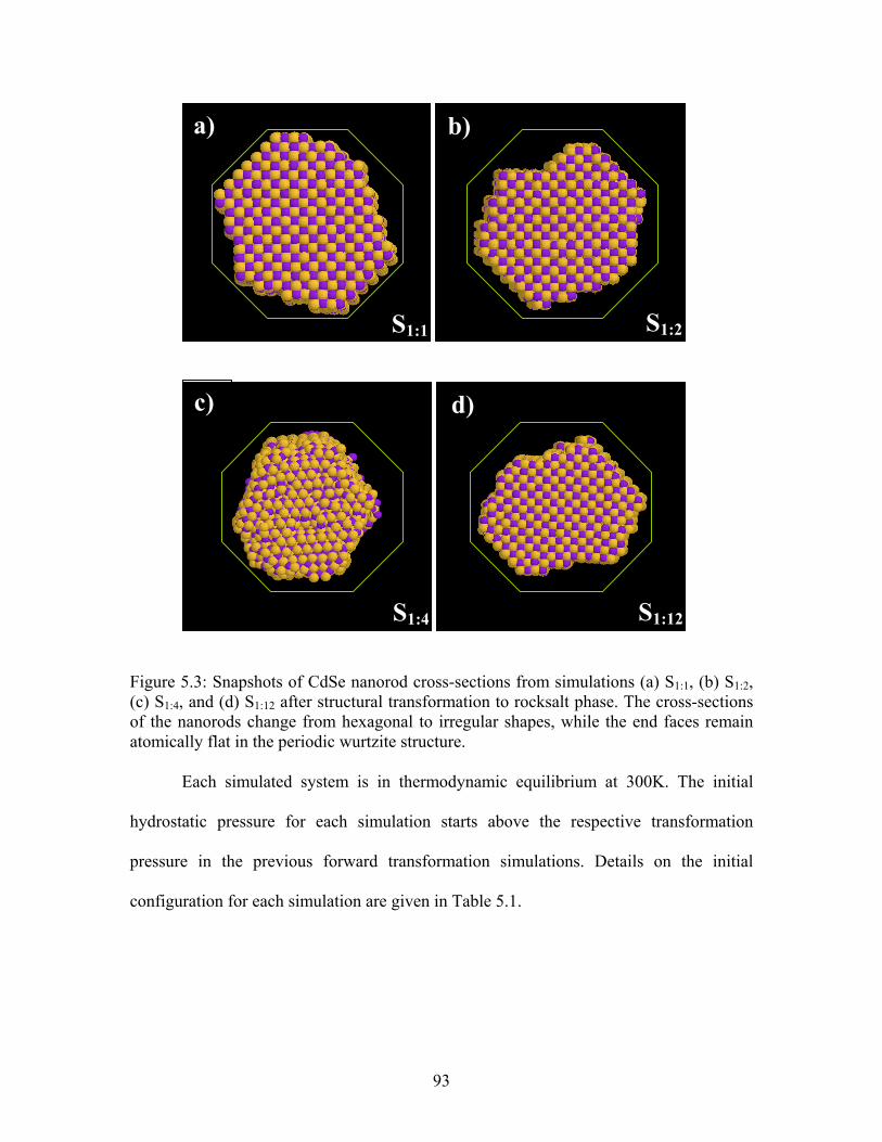
a) b)
d)c)
S1:1 S1:2
S1:12 S1:4
Figure 5.3: Snapshots of CdSe nanorod cross-sections from simulations (a) S1:1, (b) S1:2, (c) S1:4, and (d) S1:12 after structural transformation to rocksalt phase. The cross-sections of the nanorods change from hexagonal to irregular shapes, while the end faces remain atomically flat in the periodic wurtzite structure.
Each simulated system is in thermodynamic equilibrium at 300K. The initial
hydrostatic pressure for each simulation starts above the respective transformation
pressure in the previous forward transformation simulations. Details on the initial
configuration for each simulation are given in Table 5.1.
93

Table 5.1: Initial configuration parameters for “upstroke” simulations.
Simulation SU-1:1 SU-1:2 SU-1:4 SU-1:12
Rod diameter (Å) 39 – 48 37 – 46 41 – 49 41 – 57
Rod length (Å) ~35 ~79 ~164 ~484
MD cell dim. (Å, Å, Å) (94, 92, 84) (84, 94, 134) (79, 82, 294) (84, 75, 851)
Hydrostatic Pressure (GPa) 4.0 4.0 4.0 3.0
LJ fluid densities (Å-3) 0.266 0.292 0.288 0.281
# of Cd atoms 1771 3795 7463 22264
# of Se atoms 1771 3795 7463 22264
# of LJ atoms 179994 278064 473950 1252304
Total # time steps 829185 3265540 880870 818156
Total CPU time(hours) ~672 ~1800 ~828 ~389
• Simulation Procedure
Each upstroke simulation, SU-1:1, SU-1:2, SU-1:4, and SU-1:12, begins with the system at
thermodynamic equilibrium, T=300K, P>P forward transformation pressure. All MD simulations
reported in this chapter are performed in the NPT ensemble. The upstroke simulation
proceeds by a similar scheme as the down-stroke simulation. The basic schedule involves
decompression and relaxation runs executed in tandem and repeated until complete
reverse transformation or the final pressure of 0.5 MPa is reached as illustrated in the
flow chart below.
94

Decrease pressure at 0.5 GPa / 5,000 ∆t
Hold pressure constant pressure for 10,000 ∆t
Repeat until "zero" pressure
System at "zero"Pressure
NPT
Decompressed system
NPT
Relaxed configuration at new pressure
6-coordinated systemat maximum pressure
NPT
4-coordinated system
Repeat until 4-coordinated atoms dominate system
Hold system at "zero"pressure for 100,000 ∆t
Figure 5.4: Simulation schedule for the reverse transformation
Decompression runs reduce the system pressure at a rate of 5×10⁻⁵ GPa/∆t over
10,000∆t (∆t = 2fs). Relaxation runs were carried out over 2000∆t. As the density of the
LJ atoms decreased with lowering pressure, the rate of change of the MD cell volume
increased. This required slowing down the schedule to avoid unrealistic affects on the
nanorod. This will be explained later.
95

• Simulation Results for SU-1:1
Two SU-1:1 simulations, SU-1:1a and SU-1:1b, were performed as branches of SU-1:1.
Morphological changes as well as crystallographic changes were observed in both SU-1:1
simulations. Part (a) of Figure 5.5 shows the result for the SU-1:1a simulation, where the
cross section of the nanorod appears spherical in shape. The bond-angle distribution for
the nanorod at the end of SU-1:1a is broad ranging from 75° to 180° which indicates a
mixture of distorted crystalline phases. The histogram of coordinations in Figure 5.5 (c)
shows that most of the atoms in the cluster are 4-coordinated and that the number of 5-
coordinated atoms is an order of magnitude smaller than the number of 4-coordinated
atoms.
a) b)
c)
Figure 5.5: Final result of 44Å × 44Å reverse transformation, SU-1:1a. a) Snapshot of the nanorod at 180MPa and ~40,000∆t after forward transformation. b) bond-angle distribution, and c) histogram of atomic coordinations.
96

A second simulation, SU-1:1b, was performed where the temperature was kept
below 800K to prevent the nanorod from melting/deforming. Results are shown in Figure
5.6. The histogram of atomic coordination in Figure 5.6(c) shows the nanorod is
predominately 4-coordinated, but with more 5-coordinated atoms than in the first
simulation, SU-1:1a. The bond-angle distribution shows the nanorod retains rocksalt (RS)
structure. The irregular cross-section of the nanorod changes to square as the nanorod
becomes cubic. The change in the nanorods cross-section to square only occurred in the
nanorod with aspect ratio of 1:1.
a) b)
c)
Figure 5.6: Final result of the 44Å × 44Å reverse transformation, SU-1:1b. The temperature was scaled to stay below 900K. The hexagonal cross-section of the nanorod becomes rectangular. The nanorod is nearly cubic. a) Snapshot of the nanorod at 180 MPa and 500,000 ∆t after forward transformation, b) bond-angle distribution, and c) histogram of atomic coordination.
97

• Results for Simulation SU-1:2
Simulation SU-1:2 exhibits results similar to those for SU-1:1. In Figure 5.7 (b), the
bond-angle distribution indicates that the nanorod is primarily in the rocksalt phase,
although Figure 5.7 (c) shows that most of the atoms in the nanorod have become 4-fold
coordinated. The reverse transformation has started, but as with the 1x1 nanorod, the time
scale for reverse transformations appears to be much longer than that for the forward
transformation. (This result comes 3,265,540 times steps after the forward
transformation, which is roughly 75 days of CPU time!)
a) b)
c)
Figure 5.7: Final result of the 44Å × 88Å reverse transformation. a) Snapshot of the nanorod at 180MPa taken 500,000∆t after forward transformation. b) Bond-angle distribution and c) distribution of atomic coordinations.
98

• Simulation Results for SU-1:4
Simulation SU-1:4, was run for 880,870 ∆t. The results are similar to those of
simulations SU-1:1 and SU-1:2. Figure 5.8 (c) shows that the number of 4-coordinated atoms
exceeds the number of 5- and 6-coordinated atoms. The difference between the number
of 4- and 5-coordinated atoms is greater than those in the final runs for SU-1:4, SU-1:1 and
SU-1:2. This also suggests that the reverse transformation will continue to progress if the
simulation is run longer.
b)a)
c)
Figure 5.8: Final results for the reverse transformation in the 44Å × 176Å nanorod. a) Snapshot of the nanorod taken 500,000∆t after forward transformation at 180MPa. b) Bond-angle distribution and c) histogram of atomic coordinations.
99
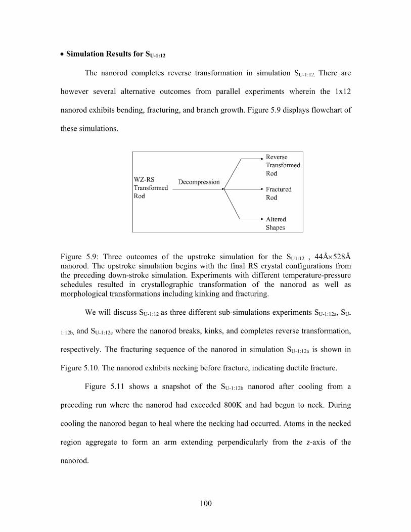
• Simulation Results for SU-1:12
The nanorod completes reverse transformation in simulation SU-1:12. There are
however several alternative outcomes from parallel experiments wherein the 1x12
nanorod exhibits bending, fracturing, and branch growth. Figure 5.9 displays flowchart of
these simulations.
Figure 5.9: Three outcomes of the upstroke simulation for the SU1:12 , 44Å×528Å nanorod. The upstroke simulation begins with the final RS crystal configurations from the preceding down-stroke simulation. Experiments with different temperature-pressure schedules resulted in crystallographic transformation of the nanorod as well as morphological transformations including kinking and fracturing.
We will discuss SU-1:12 as three different sub-simulations experiments SU-1:12a, SU-
1:12b, and SU-1:12c where the nanorod breaks, kinks, and completes reverse transformation,
respectively. The fracturing sequence of the nanorod in simulation SU-1:12a is shown in
Figure 5.10. The nanorod exhibits necking before fracture, indicating ductile fracture.
Figure 5.11 shows a snapshot of the SU-1:12b nanorod after cooling from a
preceding run where the nanorod had exceeded 800K and had begun to neck. During
cooling the nanorod began to heal where the necking had occurred. Atoms in the necked
region aggregate to form an arm extending perpendicularly from the z-axis of the
nanorod.
100

(a)
Elapsed ∆t = 0 TCd,Se,Sys = 312K, 309K, 300K P = 4.0 GPa
(b)
Elapsed ∆t = 209,500 TCd,Se,Sys = 644K, 615K, 287K P = 2.3 MPa
(c)
Elapsed ∆t = 213,500 TCd,Se,Sys = 770.K, 717K, 283K P = 1.98 MPa
(d)
Elapsed ∆t = 219,500 TCd,Se,Sys = 897K, 833K, 269K P = 0.766 MPa
(e)
Elapsed ∆t = 227,500 TCd,Se,Sys = 801K, 739K, 281K P = 0.0566MPa
Figure 5.10: The sequence of images show necking at several places along the shaft of the 44Å × 528Å nanorod until it disconnects into two pieces. a) Shows the configuration at the end of the forward transformation at 4GPa and 300K. b) Shows the nanorod ∆t later after some amount of decompression at a temperature of ~ 600K and a pressure of 2MPa. c) The nanorod begins to show noticeable necking along the shaft. The necking becomes more pronounced (d) until complete separation takes place (e).
101

Figure 5.11: A protrusion perpendicular to the axis of the nanorod results during the upstroke after the nanorod temperature increases and is then cooled down. The ability to systematically manipulate shapes of inorganic nanocrystals is an
important goal of modern chemistry and material science. The shape and size of
inorganic nanocrystals control their widely varying electrical and optical properties
[70,71,72].
Researchers have studied shape control in the synthesis of soluble and processable
CdSe nanocystals of various shapes including teardrops, arrows and tetrapods in which
ratio of surfactants, injection volume and time-dependent monomer concentration are the
controlling factors. It would be interesting to see if rapid heating and cooling can also be
used as shape-controlling factor in actual experiments and how simulation could aid those
experiments.
Figure 5.12 shows another case of the nanorod healing after necking. One part of
the nanorod kinks at a necking point to form a right angle, while the rest of the rod bends
into a curve at the other end. The necking and fracturing of the nanorods in simulations
SU-1:12a and SU-1:12b are artifacts of the method used to simulate NPT dynamics in the
upstroke sequence.
In simulation SU-1:12c, the nanorod reverts almost completely to a 4-coordinated
crystal structure. Figure 5.13 shows (a) the bond-angle distribution and (b) histogram of
102

atomic coordinations for the nanorod in the final run of simulation SU-1:12. Peaks in bond-
angle distribution are centered at 90º, 109.4º, and 180º.
Figure 5.12: The nanorod kinks at necking points after cooling during reverse transformation.
The bond-angle distribution and atomic coordination plot in Figure 5.13 indicate
that more than one crystal phase is present in the nanorod. Shell-resolved calculations for
bond-angles and atomic coordination in Figure 5.14 show different crystal phases present
in each shell. In Figure 5.14a, the red curve representing the bond-angle distribution in
the inner most shell reveals double peaks. The middle shell surrounding the innermost
shell represented by the curve in blue displays a pronounced peak at 109.4º. The curve in
103

green shows a range of angles with peaks around 90º and 180º indicating that most of the
atoms in the outer shell closer to rocksalt phase than wurtzite.
a)
b)
Figure 5.13: Final result for the reverse transformation in SU-1:12 44Å × 528Å nanorod. a) Bond-angle distribution shows peaks around 90°, 109° and 180°. The nanorod contains both rocksalt and wurtzite crystal phases. b) The histogram of atomic coordination shows a majority of 4-coordinated atoms.
Figure 5.15 shows the bond-angle distribution for the 1:12 nanorod excluding
44Å of the nanorod from each end. Peaks in each shell are now at 109.4º, which indicates
that the reverse transformation has advanced to the middle and core of the nanorod but
not to the ends yet.
104

a)
b)
Figure 5.14: Final results for the reverse transformation in the 44Å × 528Å nanorod. a) Shell-resolved bond distributions show different crystal phases in different shells. The inner-most shell, in red, indicates mixed phases. The blue curve peaks at 109°, which is characteristic of wurtzite and zinc-blende crystal structures. The outer shell represented in green shows a dominant peak at 90°, indicating mostly the rocksalt phase mixed with the wurtzite phase. b) Shows modify 4-coordinated atoms in the atomic coordination histogram
105

Figure 5.15: Peaks at 90° and 180° disappear all the curves when the atoms at the ends of the nanorod are excluded from shell-resolved bond-angle calculations. Peak at 109.4° in all shells indicates complete reverse transformation to wurtzite begins in the middle of the nanorod and spreads towards the ends.
Snapshots of the 1:12 nanorod provide further indication of how the nucleation
has occurred. In Figure 5.16 cross-sections of the nanorod cut at different segments along
the shaft are shown. Atoms with 4, 5 and 6-coordinations are represented in red, green,
and blue, respectively. Atoms with coordinations less than 3 are indicated in gray. Some
5-coordinated atoms appear near the end surfaces. However, the 4-coordinated atoms
(red) dominate the shaft of the nanorod from end to end, indicating the completeness of
reverse transformation.
(figure continued)
106

Figure 5.16: Snapshots of reverse transformation of 44Å× 528Å CdSe nanorod sliced at different cross-sections from end to end after 251,810∆t. 4, 5, 6-coodinated atoms are colored red, blue and green, respectively. 0-3 coordinated atoms are in gray. The cross-section is virtually all red along the entire core of the nanorod.
107

CHAPTER 6
CONCLUSIONS
In this thesis, we have presented molecular dynamics simulations of pressure-
induced structural phase transformations in CdSe nanorods. We conducted 4 independent
simulations. Each consisted of CdSe nanorods of various aspect ratios embedded in a
fluid pressure medium consisting of particles interacting via Lennard-Jones potential.
Simulations were performed in the NPT ensemble using the methodology developed by
Parrinello and Rahman and implemented with highly scalable multiresolution algorithms
on Beowulf parallel computing clusters.
During the simulations, the nanorods were subjected to hydrostatic pressure from
the surrounding fluid medium. All systems were taken through one pressure cycle,
beginning at ~ 0 GPa, increasing to 4.0 GPa, and then decreasing to 0.5 MPa while
maintaining constant temperature at 300K. We observe a forward transformation of the
rod during the downstroke of the cycle where each rod transforms from a 4-coordinated
wurtzite crystal structure to a 6-coordinated rocksalt structure. In the upstroke half of the
cycle, we see a reverse transformation, from a 6-coordinated rocksalt crystalline phase to
a 4-coordinated phase. In this summary we discuss results from the forward and reverse
transformation simulations as they relate to previous works and then end this chapter with
a discussion of future research.
6.1 Forward Transformation
6.1.1 Nucleation and Single Domain Formation
In this thesis we denoted the four independent simulations as S1:1, S1:2, S1:4, S1:12,
where the subscripts correspond to the width-to-length aspect ratio of the rods, with all
108

rods having a diameter of 44Å. All rods were observed to transform from pristine
wurtzite structure to a single rock-salt crystalline phase. The transformations initiated
from a single nucleation point consistent with experiments. The transformation initiates at
the surface and proceeds towards the rod axis.
6.1.2 Transformation Pressure vs. Rod Size
We have studied transformation as a function of rod length. The transformation
pressures for the CdSe nanorods decreases with increasing length from ~4.0 GPa for the
shortest nanorod (44Å in length) to ~2.5 GPa for the longest nanorod (528Å in length),
approaching the transformation pressure for bulk CdSe found by Shimojo et al. [73] from
DFT calculations. The elevation in transformation pressure with reduction in nanocrystal
size is consistent with experimental observations [74]. Additionally, the rods also
contracted by ~25% in length, which is in reasonable agreement with 18% volume
contraction in experiment on CdSe nanocrytals [75].
6.1.3 Forward Transformation Mechanism
Shimojo et al. performed simulations of pressure-induced structural
transformations in bulk CdSe using isothermal-isobaric molecular-dynamics method and
electronic-structure calculations based on the density-functional theory [76]. They
successfully reproduced reversible transformations between 4-coordinated wurtzite
structure and 6-coordinated rocksalt structures. They reported several atomistic transition
paths between CdSe wurtzite and rocksalt crystal phases RS-I or RS-II (see Figure 4.2
They also found metastable and barrier states along these transition paths. In our studies
we observed that CdSe nanorods transform from wurtzite to the RS-II crystal structure
109

and pass through a metastable state consisting of stacked flat honeycomb lattices we refer
to as, (HS) during transition.
6.2 Reverse Transformation
We investigated the reversibility of the WZ-RS transformation in a second set of
upstroke simulations SU-1:1, SU-1:2, SU-1:4, SU-1:12 (corresponding respectively to
simulations S1:1, S1:2, S1:4, S1:12). Here the pressure on the rods was reduced from 4.0 GPa
to 0.5 MPa. We observed reverse transformation to varying extents in different rods.
Nanorod size appeared to be a factor in the rate of the reverse transformation. The
number of 5-fold and 6-coordinated atoms decreased to less than the number of 4-
coordinated atoms. However, for the three shortest rods, peaks in bond angle distribution
remained practically unchanged at 90º and 180º.
Nearly a complete reverse transformation was observed only in the longest rod
SU-1:12, where the number of 4-coordinated atoms is an order of magnitude higher than the
number of 5-fold and 6-fold coordinated atoms. Bond angle distribution has a sharp peak
around 109.4º. Spatially-resolved bond angle and atomic coordination data indicate that
reverse transformation nucleates within the middle segment around the core axis of the
rod and spreads out to the shaft surface and ends.
Reverse transformation in the shorter rods is expected at longer simulation times.
However, we know from experiments that nucleation events are rare and time scale for
these events can range from picoseconds to macroscopic time scales [77]. Our longest
simulation ran for ~6.5 ns (75 days of CPU time) for simulation SU-1:2, which remained
basically in the rocksalt phase. We compare this to simulation SU-1:12 which transformed
in ~1.6 ns.
110

The reverse transformation was also accompanied by hysteresis. The cross-
sections of the nanorods changed shape from hexagonal to irregular shapes upon
compression and remained irregular in all cases except for the nanorod S1:1 which became
virtually cubic. The 1:12 nanorod showed the greatest amount of reversibility, returning
to 97% of its length in the pristine state. The smaller nanorods remained close to their
contracted, post-forward transformation lengths. Surface chemistry and topology of
nanoparticles have been shown to significantly affect internal crystal structure [78].
Perhaps we have seen this in the smaller rods, particular the S1:1 nanorod having the
highest ratio of surface-to-volume atoms.
Alivisatos’ group has studied pressure driven solid-solid phase transformations
and fracture of different shapes of CdSe nanoforms using high-pressure x-ray diffraction
and high-pressure optical absorption at room temperature. The control of shape change is
an important nanomaterial manufacturing parameter. Simulations provides insight into
the formation, fracture and structural transformations of rods and crytsals at the
nanoscale.
6.3 Future Work
We plan to develop an accelerated dynamics approach to simulate rare events in
atomistic simulations. For complex systems having large degrees of freedom, the thermal
energy fluctuations are small compared to the energy barriers for structural
transformations. Thus, the likelihood of sampling such an event is small and it may not
be feasible to observe these rare events in conventional MD simulation. Future work will
involve an implementation of action-derived molecular dynamics [79,80], which exploits
111

the knowledge of the initial and final states of a transformation and computes the
discretized path of least action between these states.
112

REFERENCES 1 Liberato Manna, Erik C. Scher, and A. Paul Alivisatos Synthesis of Soluble and Processable Rod-, Arrow-, Teardrop-, and Tetrapod-Shaped CdSe Nanocrystals 12700 J. Am. Chem. Soc. 2000, 122, 12700-12706 2 David L. Klein, P. L. M., Janet E. Bowen Katari, Richard Roth, A. Paul Alivisatos (1996). "An Approach to Electrical Studies of Single Nanocrystals Applied Physics Letters." Applied Physics Letters 68(18). 3 Chieh-Ju Lee, A. M., Uri Banin, Marvin L. Cohen, A. P. Alivisatos (2000). "Observation of Pressure-Induced Direct-to-Indirect Band Gap Transition in InP Nanocrystals." Journal of Chemical Physics 113(5): 2016-2020. 4 L. G. Wang, P. K., N. Moll and M. Scheffler (2000). "Size, Shape, and Stability of InAs Quantum Dots on the Gas As(001) Substrate." Physics Review B 62(3): 1897-1904. 5 Hedi Mattoussi, J. M. M., Ellen R. Goldman, George P. Anderson, and F. V. M. Vikram C. Sundar, and Moungi G. Bawendi (2000). "Self-Assembly of CdSe-ZnS Quantum Dot Bioconjugates Using an Engineered Recombinant Protein." Journal of the American Chemical Society 122: 12142-12150. 6 B. O. Dabbousi, J. R.-V., F. V. Mikulec, J. R. Heine, H. Mattoussi, R. Ober, K. F. Jensen, and M. G. Bawendi (1997). "(CdSe)ZnS Core-Shell Quantum Dots: Synthesis and Characterization of a Size Series of Highly Luminescent Nanocrystallites." J. Phys. Chem. B 101: 9463-9475. 7 Fuyuki Shimojo, S. K., Ingvar Ebbsjö, Rajiv Kalia, Aiichiro Nakano, and Priya Vashishta (2004). "Atomic Mechanisms for Wurtzite-to-Rocksalt Structural Transformation in Cadmium Selenide under Pressure." Physical Review B 70: 184111-1 to 184111-6. 8 Anderson (1980). "Molecular Dynamics Simulations at Constant Pressure and Temperature." J. Chem. Phys. 72(4): 2384-2393. 9 H. Tanaka, K. N. a. N. W. (1983). Ibid. 78: 2626. 10 Nose, S. (1984). "A Molecular-Dynamics Method for Simulations in the Canonical Ensemble." Molecular Physics 52(2): 255 - 268. 11 Ibid. 12 Anderson (1980). "Molecular Dynamics Simulations at Constant Pressure and Temperature." J. Chem. Phys. 72(4): 2384-2393.
113

13 Rahman, P. a. (1981). J. Appl. Phys. 52: 7182. 14 S. Kodiyalam, R. K., et al (2001). "Grain Boundaries in Gallium Arsenide Nanocrystals Under Pressure: A Parallel Molecular-Dynamics Study." Physical Review Letters 86(1): 55-58. 15 F. Shimojo, I. E., et al. (2000). "Molecular Dynamics Simulation of Structural Transformation in Silicon Carbide under Pressure." Ibid. 84(15): 3338. 16 J. P. Rino, A. C., I. Ebbsjö , R. Kalia,A. Nakano, F.Shimojo, P. Vashishta (2002). Phys. Rev. B 65. 17 A. F. Voter (1996). Materials Research Society Bulletin 21: 17. 18 Tersoff, J. (1989). Phys. Rev. B 39: 5566. 19 Weber, F. H. S. a. T. A. (1985). Ibid. 31(5262). 20 Satyavani Vemparala, R. K. K., Aiichiro Nakano, and Priya Vashishta (2004). "Electric field induced switching of poly.ethylene glycol. terminated self-assembled monolayers: A parallel molecular dynamics simulation." JOURNAL OF CHEMICAL PHYSICS 121(11): 5427-5433. 21 Rokhlin, L. G. a. V. (1987). "A Fast Algorithm for Particle Simulations." J. Comp. Phys. 73. 22 Gear, C. W. (1966). The Numerical Integration of Ordinary Differential Equations of Various Orders. Chicago, Argonne National Laboratory. 23 Gear, C. W. (1971). The Numerical Initial Value Problems in Ordinary Differential Equations. Englewood Cliffs, NJ, Prentice-Hall. 24 Verlet, L. (1967). Phys. Rev. 159(98). 25 Nose, S. (1984). "A Unified Formulation of the Constant Temperature Molecular- Dynamics Methods." Journal of Chemical Physics 81(1): 511 - 519. 26 G.J. Martyna, M. T., B.J. Berne (1992). "Reversible Multiple Time Scale Molecular Dynamics." J. Chem. Phys. 97(3): 1990-2001. 27 Anderson (1980). "Molecular Dynamics Simulations at Constant Pressure and Temperature." Ibid. 72(4): 2384-2393.
114

28 Parrinello (1980). "Crystal Structure and Pair Potential: A Molecular-Dynamics Study." Physics Review Letters 45(14): 1196-1199. 29 Glenn J. Martyna, M. E. T., Douglas J. Tobias and Micheal L. Klein (1996). "Explicit Reversible Integrators for Extended Systems Dynamics." Molecular Physics 87(5): 1117-1157. 30 Duan, Y. K., P.A (1998). "Pathways to a protein folding intermediate observed in a 1-microsecond simulation in aqueous solution." Science 282: 740-744. 31 Kollman, P. A., et al, Cheatham, T.E. III. (2000). "Calculating structures and free energies of complex molecules: Combining molecular mechanics and continuum models." Acc. Chem. Res. 33: 889-897. 32 Brooks B. B., B. R. E., Olafson B. D., States D. J., Swaminathan S., Karplus M. (1983). "CHARMM: A program for macromolecular energy, minimization and dynamics calculations." J. Comp. Chem. 4: 187. 33 Cornell W. D., C. P., Bayly C. I., Gould I. R., Merz K. M., Ferguson D. M., and F. T. Spellmayer D. C., Caldwell J. W., Kollman P. A. (1995). "A second generation force field for the simulation of proteins, nucleic acids, and organic molecules." J. Am. Chem. Soc. 117: 5179. 34 van Gunsteren W. F., B. H. J. C. (1988). GROMOS: GROningen MOLecular Simulation software. Groningen, Netherlands, University of Groningen. 35 Raine, A. C., Fincham, D. and Smith, W. "1989." Comp. Phys. Comm. 55: 13. 36 Plimpton, S. J. (1995). "Fast Parallel Algorithms for Short-Range Molecular Dynamics." J Comp Phys 117: 1-19. 37 Rapaport, D. C. (1995). The Art of Molecular Dynamics Simulation. Cambridge, MA, Cambridge Univ. Press. 38 S. Froyen and M.L. Cohen, Phys. Rev. B 28, 3258 (1983) 39 Hengzhong Zhang, Benjamin Gilbert, Feng Huang & Jillian F. Banfield, Nature 424, 1025 - 1029 (28 August 2003); Hhttp://www.nature.com/nature/journal/v424/n6952/full/nature01845_fs.htmlH 40 Satyavani Vemparala, Rajiv K. Kalia, Aiichiro Nakano, and Priya Vashishta Electric field induced switching of poly(ethylene glycol) terminated self-assembled monolayers: A parallel molecular dynamics simulation, J. Chem. Phys. Vol. 121, No. 11
115

41 Shimojo, F., I. Ebbsjo, et al. (2000). Physical Review Letters 84: 3338. 42 Sowa, H. (2000). Zeishrift Fur Kristallography 215(315). 43 Sharma, S. M. and Y. M. Gupta (1998). Physical Review B58: 5964. 44 Knudson, M. D., Y. M. Gupta, et al. (1999). Ibid. B59: 11704. 45 Limpijumnong, S. and W. R. L. Lambrecht (2001). Physical Review Letters 86: 91. 46 Ibid. 47 Sowa, H. (2001). Acta Cryst. A57: 176. 48 Wilson, M. and P. A. Madden (2002). Journal of Physics: Condensed Matter 14: 4629. 49 F. Shimojo, S. Kodiyalam, I. Ebbsjö, R. Kalia, A. Nakano, P. Vashishta Phys. Rev. B 70, 184111 (2004) 50 Fuyuki Shimojo, S. K., Ingvar Ebbsjö, Rajiv Kalia, Aiichiro Nakano, and Priya Vashishta (2004). "Atomic Mechanisms for Wurtzite-to-Rocksalt Structural Transformation in Cadmium Selenide under Pressure." Physical Review B 70: 184111-1 to 184111-6. 51 S. Tolbert, A.P. Alivisatos, J. Chem. Phys. Vol. 102, No. 11 52 J. Wickham, A. Herhold, A.P. Alivisatos, Phys. Rev. Lett. 84, 5 (2000) 53 D. Zaziski, S. Prilliman, E. Scher, M. Casula, J. Wickham, S. Clark, A.P. Alivisatos, Nanoletters, Vol. 4, No. 5 943-946 (2004) 54 Jacobs, K., D. Zaziski, et al. (2001). Science 293(1803). 55 Tolbert, S. H. and A. P. Alivisatos (1994). "Science." 265(373). 56 Shimojo, F., I. Ebbsjo, et al. (2000). Physical Review Letters 84: 3338. 57 Sowa, H. (2000). Zeishrift Fur Kristallography 215(315). 58 Sharma, S. M. and Y. M. Gupta (1998). Physical Review B58: 5964. 59 Knudson, M. D., Y. M. Gupta, et al. (1999). Ibid. B59: 11704. 60 Limpijumnong, S. and W. R. L. Lambrecht (2001). Physical Review Letters 86: 91.
116

61 Ibid. 62 Sowa, H. (2001). Acta Cryst. A57: 176. 63 Wilson, M. and P. A. Madden (2002). Journal of Physics: Condensed Matter 14: 4629. 64 Karl Johnson, A. Z., Keith Gubbins (1992). "Lennard-Jones Equation of State Revisted." Molecular Physics 78: 591-618. 65 S. Kodiyalam, R. K., et al (2001). "Grain Boundaries in Gallium Arsenide Nanocrystals Under Pressure: A Parallel Molecular-Dynamics Study." Physical Review Letters 86(1): 55-58. 66 Karl Johnson, A. Z., Keith Gubbins (1992). "Lennard-Jones Equation of State Revisted." Molecular Physics 78: 591-618. 67 Ibid. 68 Philip S. Antón, R. S., and James Schneider (2001). The Global Technology Revolution:Bio/Nano/Materials Trends and Their Synergies with Information Technology by 2015, RAND Corporation. 69 Alivisatos, A. P. (2004). "Critical Size for Fracture during Solid-Solid Phase Transformations." NANO LETTERS 4(5): 943-946. 70Alivisatos, A. P. (1996). Science 271: 933-937. 71 Lieber, C. M. Solid State Communications 107: 607-616. 72 Smalley, R. E. Y., B. I. (1998). Solid State Commun. 107: 597-606. 73 Fuyuki Shimojo, S. K., Ingvar Ebbsjö, Rajiv Kalia, Aiichiro Nakano, and Priya Vashishta (2004). "Atomic Mechanisms for Wurtzite-to-Rocksalt Structural Transformation in Cadmium Selenide under Pressure." Physical Review B 70: 184111-1 to 184111-6. 74 S. Tolbert, A. B. H., L. E. Brus, A. P. Alivisatos (1995). "Pressure-Induced Structural Transformations in Si Nanocrystals: Surface and Shape Effects." Physical Review Letters 76(23). 75 K. Jacobs, D. Z., E. C. Scher, A. B. Herhold, A. Paul Alivisatos (2001). "Activation Volumes for Solid-Solid Transformations in Nanocrystals." Science 293. 76 Fuyuki Shimojo, S. K., Ingvar Ebbsjö, Rajiv Kalia, Aiichiro Nakano, and Priya Vashishta (2004). "Atomic Mechanisms for Wurtzite-to-Rocksalt Structural
117

Transformation in Cadmium Selenide under Pressure." Physical Review B 70: 184111-1 to 184111-6. 77 Alivisatos, A. P. (2004). "Critical Size for Fracture during Solid-Solid Phase Transformations." NANO LETTERS 4(5): 943-946. 78 Hengzhong Zhang, B. G., Feng Huang , Jillian F. Banfield (2003). "Surface chemistry and topology of nanoparticles and has a significant effect on crystal structure." Nature 424: 1025-1028. 79 Parrinello, D. P. M. (2001). "Action-Derived Molecular Dynamics in the Study of Rare Events." Physical Review Letters 87(10). 80 Huber, B. A. G. T. (2004). "Long time scale molecular dynamics using least action." Australian & New Zealand Industrial and Applied Mathematics Journal 44(E): C534,C550.
118

VITA
Nicholas Jabari Ouma Lee was born on August 2, 1973, in Jackson, Mississippi,
to Verna and Nathaniel Lee. Jabari graduated from the Callaway High School and the
Academic and Performing Arts Complex in Jackson, Mississippi, in June 1991 and
enrolled at Jackson State University where he majored in physics. Jabari was privileged
to work under the mentorship of Dr. Kunal Ghosh on describing frequency-dependent
behavior of dielectric properties of porous media. He graduated from Jackson State
University with a Bachelor of Science degree from the Department of Physics and
Atmospheric Sciences and was awarded a fellowship from the David and Lucille Packard
Foundation in 1995.
In August 1997, Jabari entered the doctoral program in physics at Louisiana State
University where he was awarded a National Science Foundation Graduate Research
Traineeship. He joined the Concurrent Computing Laboratory for Materials Simulations
at that time. He was awarded a Master of Science in physics from Louisiana State
University in December 2000. He currently lives in Los Angeles, California. His future
plans include pursing a post-doctoral position after receiving the degree of Doctor of
Philosophy in December 2005.
119