Embed Size (px)
Citation preview

TR-CS-97-10
Parallel Integer Sorting
Andrew Tridgell, Richard Brentand Brendan McKay
May 1997
Joint Computer Science Technical Report Series
Department of Computer ScienceFaculty of Engineering and Information Technology
Computer Sciences LaboratoryResearch School of Information Sciences and Engineering

This technical report series is published jointly by the Department ofComputer Science, Faculty of Engineering and Information Technology,and the Computer Sciences Laboratory, Research School of InformationSciences and Engineering, The Australian National University.
Please direct correspondence regarding this series to:
Technical ReportsDepartment of Computer ScienceFaculty of Engineering and Information TechnologyThe Australian National UniversityCanberra ACT 0200Australia
or send email to:
A list of technical reports, including some abstracts and copies of some fullreports may be found at:
http://cs.anu.edu.au/techreports/
Recent reports in this series:
TR-CS-97-09 M. Manzur Murshed and Richard P. Brent. Constant timealgorithms for computing the contour of maximal elements on theReconfigurable Mesh. May 1997.
TR-CS-97-08 Xun Qu, Jeffrey Xu Yu, and Richard P. Brent. A mobile TCPsocket. April 1997.
TR-CS-97-07 Richard P. Brent. A fast vectorised implementation of Wallace’snormal random number generator. April 1997.
TR-CS-97-06 M. Manzur Murshed and Richard P. Brent. RMSIM: a serialsimulator for reconfigurable mesh parallel computers. April 1997.
TR-CS-97-05 Beat Fischer. Collocation and filtering — a data smoothingmethod in surveying engineering and geodesy. March 1997.
TR-CS-97-04 Stephen Fenwick and Chris Johnson. HeROD flavouredoct-trees: Scientific computation with a multicomputer persistentobject store. February 1997.

Parallel Integer Sorting
Andrew Tridgell, Richard Brent and Brendan McKay
Department of Computer Science
Australian National University
December 13, 1995

Contents
1 Introduction 3
2 Internal sorting 4
2.1 Overview of the algorithm : : : : : : : : : : : : : : : : : : : : : : 42.2 Distribution requirements : : : : : : : : : : : : : : : : : : : : : : 52.3 Local sorting : : : : : : : : : : : : : : : : : : : : : : : : : : : : : 5
2.3.1 Quicksort : : : : : : : : : : : : : : : : : : : : : : : : : : : 52.3.2 Radix sort : : : : : : : : : : : : : : : : : : : : : : : : : : : 62.3.3 American ag sort : : : : : : : : : : : : : : : : : : : : : : 6
2.4 Merge exchange operation : : : : : : : : : : : : : : : : : : : : : : 72.4.1 The Find-Exact Algorithm : : : : : : : : : : : : : : : : : 72.4.2 Unbalanced Merging : : : : : : : : : : : : : : : : : : : : : 92.4.3 Blockwise Merging : : : : : : : : : : : : : : : : : : : : : : 10
2.5 Primary merge : : : : : : : : : : : : : : : : : : : : : : : : : : : : 112.6 Cleanup : : : : : : : : : : : : : : : : : : : : : : : : : : : : : : : : 13
3 External sorting 14
3.1 Lower Limits on I/O : : : : : : : : : : : : : : : : : : : : : : : : : 143.2 Overview of the algorithm : : : : : : : : : : : : : : : : : : : : : : 153.3 Partitioning : : : : : : : : : : : : : : : : : : : : : : : : : : : : : : 153.4 Column and row sorting : : : : : : : : : : : : : : : : : : : : : : : 173.5 Completion : : : : : : : : : : : : : : : : : : : : : : : : : : : : : : 173.6 Processor allocation : : : : : : : : : : : : : : : : : : : : : : : : : 183.7 Large k : : : : : : : : : : : : : : : : : : : : : : : : : : : : : : : : 183.8 Other partitionings : : : : : : : : : : : : : : : : : : : : : : : : : : 19
4 Performance 20
4.1 The test environment : : : : : : : : : : : : : : : : : : : : : : : : 204.2 Serial sorting : : : : : : : : : : : : : : : : : : : : : : : : : : : : : 204.3 Internal parallel sorting : : : : : : : : : : : : : : : : : : : : : : : 234.4 External sorting : : : : : : : : : : : : : : : : : : : : : : : : : : : 25
4.4.1 IO E�ciency : : : : : : : : : : : : : : : : : : : : : : : : : 264.4.2 Worst case : : : : : : : : : : : : : : : : : : : : : : : : : : 28
5 Conclusions 30
6 Source code 30
6.1 Using the test program : : : : : : : : : : : : : : : : : : : : : : : : 30

1 Introduction
This paper presents algorithms and experiments for internal (in core) and exter-nal (secondary memory) parallel sorting. It concentrates on algorithms appro-priate for medium scale MIMD parallel computers, with all experiments beingperformed on a 128 processor Fujitsu AP1000.
Data sizes ranging from a few hundred thousand to a few hundred millionelements are considered, with all elements being either 64 bit or 128 bit integers.
The internal sorting algorithm is based on earlier work by Andrew Tridgelland Richard Brent[11], while the external sorting algorithm was developed forthis paper.
The paper also takes a quick look at serial sorting algorithms, as they playan important part as subroutines in the parallel sorting algorithms.
3

2 Internal sorting
Internal parallel sorting just means sorting data which �ts in the parallel ma-chines primary memory without resorting to secondary memory. It is not di�-cult to come up with a parallel sorting algorithm that is asymptotically optimal(any local sort then merge algorithm will do) but it can be quite hard to �ndan algorithm that actually a achieves a reasonable percentage of the optimal Ptimes speedup for reasonable data sizes.
This paper describes a local-sort/merge algorithm which uses a number ofalgorithmic tricks to achieve quite respectable performance over a wide rangeof parameters. It was �rst described in [11].
2.1 Overview of the algorithm
The internal sorting algorithm is basically a simple parallel merge sort. Eachprocessor sorts its own elements using a local sorting algorithm then the proces-sors perform a series of merge-exchange operations to bring the locally sortedlists into globally sorted order.
The novel parts of the algorithm are in the choice of the pattern of mergeexchange operations, and the implementation details of the merge-exchangeoperation itself. Together these lead to a highly e�cient algorithm that performswell under a wide range of circumstances.
The pattern of merge exchanges is split into two parts. In the �rst part,called the primary merge, a highly parallelisable hypercube algorithm is usedthat \almost sorts" the data. The algorithm produces a ordering of the datawhich is close to being completely sorted but needs some cleanup operations.
The second part, called the cleanup, consists of merge exchange operationsfollowing the pattern of Batcher's merge exchange sort[6]. This algorithm hasthe property that it completes very quickly for almost sorted data, and thus isideal as a cleanup operation.
The merge exchange operation itself is also split into a number of parts. Inthe �rst part, which we call \�nd-exact", the two processors exchange individualelements in a bisection search to �nd which elements need to be transferredbetween the processors. The processors then do a bulk swap of elements basedon the result of the �nd-exact operation.
Each processor taking part in the merge-exchange then has two lists of ele-ments and needs to perform a local merge-exchange between them. This mergeexchange can take advantage of the position of the lists after the bulk swap ofelements to produce a fast memory e�cient block-wise merge algorithm.
In the following sections each of the stages of the internal sorting algorithmis described. A more detailed and general account of the algorithm can also befound in [11].
4

2.2 Distribution requirements
The algorithm described below will assume that the elements start out dis-tributed across the processors. It will also assume a particular packing of theelements on the processors. The packing that is required is described as follows
Np+1 � Np
If Np+1 > 0 then Np = Np�1
where Np is the number of elements on processor p and p is restricted to suitableranges.
This packing is a result of \in�nity padding" where virtual in�nity elementsare added to the data to bring the total number of elements up to a multipleof the number of processors P . These virtual in�nity elements must be initiallyplaced in the highest cell numbers to guarantee that they will not have to moveduring the sorting process.
An algorithm for e�ciently obtaining the required initial distribution is de-scribed in [11].
2.3 Local sorting
The choice of algorithm for sorting the elements within each cell is perhaps thesimplest part of the process. As the results will show, however, it is critical tothe overall performance of the algorithm.
A simple demonstration of the importance of the serial sorting phase can bemade by calculating its expected contribution to the total time for the parallelsorting algorithm under some simple assumptions.
If we assume that the serial sorting algorithm takes time N logN then wewould expect an ideal parallel sorting algorithm to take N logN
P. The local
sorting portion of the algorithm (executed in parallel) would take NPlog N
P. This
means we would expect the serial sorting phase of the algorithm to take 1� logPlogN
of the total time.If we assume we have 27 processors and 230 elements then we would ex-
pect the serial sorting phase to take more than 75% of the total sorting time.Obviously the choice of serial sorting algorithm is critical.
2.3.1 Quicksort
A very commonly used serial sorting algorithm is quicksort. Quicksort is acomparison based in-place serial sorting algorithm based around partitioning.It is often included (in a slightly modi�ed form) in a standard C library functionqsort(). The problem is that the C library implementations are typically veryslow.
5
The main problem is that they call a user de�ned function for each com-parison. A huge speed improvement can often be had by inlining the compari-son function. Further improvements can be made by tuning the insertion sortthreshold, which is the point at which the algorithm switches to a fast insertionsort for small numbers of elements.
For this paper the GNU quicksort implementation was investigated, usinginlined comparisons. It was found to be much faster than the standard libraryroutines.
2.3.2 Radix sort
When sorting integers or integer-like quantities a considerable advantage can begained from the bitwise ordering of the elements. The best known algorithm totake advantage of this is radix sort. In its simplest form a radix sort is a bucketsort which �rst partitions using the least signi�cant bits then progressively par-titions for the more signi�cant bits of the data.
Typically 8 bits are considered at one time for convenience of programming.This means that for 128 bit integers the algorithm requires 16 passes through thedata, with each pass doing essentially random accesses. This leads to very poorperformance. Radix sorts perform very well for small integers (up to around 32bits or so) but degrade rapidly beyond that.
Radix sorts also typically require temporary storage of approximately equalsize to the input data. As will become plain later, this is unacceptable forparallel sorting in many cases, especially for external parallel sorting.
2.3.3 American ag sort
Another class of radix sorting algorithms are the forward radix sorts. Theseexamine the most signi�cant bits �rst and do a successive partitioning movingtowards the less signi�cant bits. This has the big advantage that the sort canstop when enough bits have been examined to sort the data (for N elements thiswill typically be around logN bits for random data). This makes it much moreattractive for sorting 128 bit elements.
The problem with forward radix sorts is that they commonly produce lotsof empty buckets in the later passes of the sort which leads to large overheadsin bucket management.
The American ag sort[12] is a �ne tuned forward radix sort. It uses algorith-mic and programming tricks to largely avoid the problems of empty buckets, andalso manages to produce a in-place radix sort using a sophisticated tail-chasingalgorithm. It performs very well over a very wide range of parameters.
The standard American ag sort is designed for NULL terminated, variablelength strings, and uses an array of pointers to the strings as the \elements".For this paper the algorithm was modi�ed to sort �xed length integers without
6
the use of an array of pointers. The changes required to do this were quitesmall.
The American ag sort was chosen as the principle serial sorting algorithmfor the results later in this paper.
2.4 Merge exchange operation
The aim of the merge-exchange operation is to exchange elements between twoprocessors so that we end up with one processor containing elements which areall smaller than all the elements in the other processor, while maintaining theorder of the elements in the processors. In our implementation of parallel sortingwe always require the processor with the smaller processor number to receivethe smaller elements. 1
Secondary aims of the merge-exchange operation are that it should be veryfast for data that is almost sorted already, and that the memory overhead shouldbe minimised. 2
Suppose that a merge operation is needed between two processors, 1 and 2,which initially contain N1 and N2 elements respectively. We assume that thesmaller elements are required in processor 1 after the merge.
In principle, merging two already sorted lists of elements to obtain a newsorted list is a very simple process. The pseudo-code for the most naturalimplementation is shown in Figure 1
This algorithm completes in N1+N2 steps, with each step requiring one copyand one comparison operation. The problem with this algorithm is the storagerequirements implied by the presence of the destination array. This means thatthe use of this algorithm as part of a parallel sorting algorithm would restrictthe number of elements that can be sorted to the number that can �t in halfthe available memory of the machine. The question then arises as to whetheran algorithm can be developed that does not require this destination array.
In order to achieve this, it is clear that the algorithm must re-use the spacethat is freed by moving elements from the two source lists. We now describe howthis can be done. The algorithm has several parts, each of which is describedseparately.
2.4.1 The Find-Exact Algorithm
When a processor takes part in a merge-exchange with another processor, it willneed to be able to access the other processors elements as well as its own. The
1This would not be possible if we used Batcher's bitonic algorithm instead of his merge-exchange algorithm for the cleanup phase. The bitonic algorithm is not a unidirectionalalgorithm, it requires elements to be moved away from their �nal destination at some stages.
2The minimisation of the memory overhead becomes important when the internal parallelsorting algorithm is later used as a subroutine for the external algorithm, where memory isat a premium
7

procedure merge(list dest, list source1, list source2)
while (source1 not empty) and (source2 not empty)
if (top_of_source1 < top_of_source_2)
put top_of_source1 into dest
else
put top_of_source2 into dest
endif
endwhile
while (source1 not empty)
put top_of_source1 into dest
endwhile
while (source2 not empty)
put top_of_source2 into dest
endwhile
end
Figure 1: Pseudo-code for a simple merge
simplest method for doing this is for each processor to receive a copy of all ofthe other processors elements before the merge begins.
A much better approach is to �rst determine exactly how many elementsfrom each processor will be required to complete the merge, and to transferonly those elements. This reduces the communications cost by minimising thenumber of elements transferred, and at the same time reduces the memoryoverhead of the merge.
The �nd-exact algorithm allows each processor to determine exactly howmany elements are required from another processor in order to produce thecorrect number of elements in a merged list.
Say we have two processors, called processor 1 and processor 2, which eachhave N elements.3 We want to �nd which of these 2N elements will need toend up in the �rst cell and which in the second.
If we label the two lists of elements E1;i and E2;i then when a comparisonis made between element E1;A�1 and E2;N�A then the result of the comparisondetermines whether processor 1 will require more or less than A of its ownelements in the merge. If E1;A�1 is greater than E2;N�A then the maximumnumber of elements that could be required to be kept by processor 1 is A � 1,otherwise the minimum number of elements that could be required to be keptby processor 1 is A.
The proof that this is correct relies on counting the number of elements that
3A generalisation to the case where the number of elements in each cell is not the same isgiven in [11]
8

could be less than E1;A�1. If E1;A�1 is greater than E2;N�A then we know thatthere are at least N �A+ 1 elements in processor 2 that are less than E1;A�1.If these are combined with the A� 1 elements in processor 1 that are less thanE1;A�1, then we have at least N elements less than E1;A�1. This means thatthe number of elements that must be kept by processor 1 must be at most A�1.
A similar argument can be used to show that if E1;A�1 � E2;N�A then thenumber of elements to be kept by processor 1 must be at least A. Combin-ing these two results leads to an algorithm that can �nd the exact number ofelements required in at most logN steps by successively halving the range ofpossible values for the number of elements required to be kept by processor 1.
Once this result is determined it is a simple matter to derive from this thenumber of elements that must be sent from processor 1 to processor 2 and fromprocessor 2 to processor 1.
On a machine with a high message latency, this algorithm could be costly, asa relatively large number (ie. up to logN) of small messages are transferred. Thecost of the algorithm can be reduced, but with a penalty of increased messagesize and algorithm complexity. To do this the processors must exchange morethan a single element at each step, sending a tree of elements with each leafof the tree corresponding to a result of the next several possible comparisonoperations. This method has not been implemented as the practical cost of the�nd-exact algorithm was found to be very small on the target machine.
We assume for the remainder of the discussion on the merge-exchange algo-rithm that after the �nd exact algorithm has completed it has been determinedthat processor 1 must retain L elements and must transfer N �L elements fromprocessor 2.
2.4.2 Unbalanced Merging
Before considering the algorithm that has been devised for minimum memorymerging, it is worth considering a special case where the result of the �nd-exactalgorithm determines that the number of elements to be kept on processor 1 ismuch larger than the number of elements to be transferred from processor 2.
In this case the task which processor 1 must undertake is to merge two listsof very di�erent sizes. There is a very e�cient algorithm for this special case.
Suppose that L is much greater than N � L. This may occur if the data isalmost sorted, for example, near the end of the cleanup phase.4 We proceed asfollows.
First we determine, for each of the N�L elements that have been transferredfrom 1, where it belongs in the list of length L. This can be done with at most(N � L) logL comparisons using a method similar to the �nd-exact algorithm.
4Experiments have shown that this is a very common occurrence, and the implementationof this as a special case improves the overall performance of the parallel sorting algorithmsigni�cantly
9

As N � L is small, this number of comparisons is small, and the results takeonly O(N � L) storage.
Once this is done we can copy all the elements in list 2 to a temporary storagearea and begin the process of slotting elements from list 1 and list 2 into theirproper destinations. This takes at most N element copies, but in practice itoften takes only about 2(N �L) copies. This is explained by the fact that whenonly a small number of elements are transferred between processors there is oftenonly a small overlap between the ranges of elements in the two processors, andonly the elements in the overlap region have to be moved. Thus the unbalancedmerge performs very quickly in practice, and the overall performance of thesorting procedure is signi�cantly better than it would be if we did not takeadvantage of this special case.
2.4.3 Blockwise Merging
The blockwise merge is a solution to the problem of merging two sorted lists ofelements into one, while using only a small amount of additional storage. The�rst phase in the operation is to break the two lists into blocks of an equal sizeB. The exact size of B is unimportant for the functioning of the algorithm andonly makes a di�erence to the e�ciency and memory usage of the algorithm.We assume that B is O(
pN), which is small relative to the memory available on
each processor. To simplify the exposition we also assume, for the time being,that L and N � L are multiples of B.
The merge takes place by merging from the two blocked lists of elementsinto a destination list of blocks. The destination list is initially primed withtwo empty blocks which comprise a temporary storage area. As each block inthe destination list becomes full the algorithm moves on to a new, empty block,choosing the next one in the destination list. As each block in either of the twosource lists becomes empty they are added to the destination list.
As the merge proceeds there are always exactly 2B free spaces in the threelists. This means that there must always be at least one free block for thealgorithm to have on the destination list, whenever a new destination block isrequired. Thus the elements are merged completely with them ending up in ablocked list format controlled by the destination list.
The algorithm actually takes no more steps than the simple merge outlinedearlier. Each element moves only once. The drawback, however, is that thealgorithm results in the elements ending up in a blocked list structure ratherthan in a simple linear array.
The simplest method for resolving this problem is to go through a re-arrangement phase of the blocks to put them back in the standard form. This iswhat has been done in the implementation of our parallel sorting algorithm. Itwould be possible, however, to modify the whole algorithm so that all referencesto elements are performed with the elements in this block list format. At thisstage the gain from doing this has not warranted the additional complexity, but
10

procedure primary_merge(integer base, integer num)
if num = 1 return
for all i in [0..num/2)
merge_exchange (base+i, base+i+(num+1)/2)
primary_merge (base+num/2, (num+1)/2)
primary_merge (base, num - (num+1)/2)
end
Figure 2: Pseudo-code for primary merge
if the sorting algorithm is to attain its true potential then this would becomenecessary.
As mentioned earlier, it was assumed that L and N �L were both multiplesof B. In general this is not the case. If L is not a multiple of B then thisintroduces the problem that the initial breakdown of list 2 into blocks of sizeB will not produce blocks that are aligned on multiples of B relative to the�rst element in list 1. To overcome this problem we must make a copy of theL mod B elements on the tail of list 1 and use this copy as a �nal source block.Then we must o�set the blocks when transferring them from source list 2 to thedestination list so that they end up aligned on the proper boundaries. Finally wemust increase the amount of temporary storage to 3B and prime the destinationlist with three blocks to account for the fact that we cannot use the partial blockfrom the tail of list 1 as a destination block.
Consideration must �nally be given to the fact that in�nity padding mayresult in a gap between the elements in list 1 and list 2. This can come aboutif a processor is keeping the larger elements and needs to send more elementsthan it receives. Handling of this gap turns out to be a trivial extension of themethod for handling the fact that L may not be a multiple of B. We just add anadditional o�set to the destination blocks equal to the gap size and the problemis solved.
2.5 Primary merge
The aim of the primary merge phase of the algorithm is to almost sort thedata in minimum time. For this purpose an algorithm with a very high parallele�ciency was chosen to control merge-exchange operations between the nodes.This led to signi�cant performance improvements over the use of an algorithmwith lower parallel e�ciency that is guaranteed to completely sort the data (forexample, Batcher's algorithm as used in the cleanup phase).
The pattern of merge-exchange operations in the primary merge consists ofmerge-exchange operations along the edges of a hyper-cube. The pseudo-codefor the algorithm is given in Figure 2. When the algorithm is called the base is
11

Figure 3: The parallelisation of the primary merge for P = 8
initially set to the index of the smallest node in the system and num is set tothe number of nodes, P .
Note that the algorithm is only a true hyper-cube algorithm for when P isa power of 2. In other cases the algorithm can be thought of as a incompletehyper-cube, and will lead to less parallel e�ciency than can be achieved with apower of 2.
This algorithm completes in logP steps per node, with each step consistingof a merge-exchange operation between two processors as described above. IfP is not a power of 2 then a single node may be left idle at each step of thealgorithm, with the same node never being left idle twice in a row.
If P is a power of 2 and the initial distribution of the elements is random, thenat each step of the algorithm each node has about the same amount of work toperform as the other nodes. In other words, the load balance between the nodesis very good. The symmetry is only broken due to an unusual distribution of theoriginal data, or if P is not a power of 2. In both these cases load imbalancesmay occur.
Figure3 shows the parallelisation of the primary merge for P = 8. The �gureis layed out with time on the vertical axis. On the horizontal axis are evenlyspaced points for each processor. An arrow going from processor 4 to processor0 means that a merge exchange takes place between those two processors withthe smaller elements ending up in processor 0.
The dashed line separates stages of the sort which can be completed com-pletely in parallel. Thus the primary merge for P = 8 takes 3 parallel steps tocomplete. In fact, this algorithm will always take dlog2 P e parallel steps.
12

2.6 Cleanup
The cleanup phase of the algorithm is similar to the primary merge phase, but itmust be guaranteed to complete the sorting process. The method that has beenchosen to achieve this is Batcher's merge-exchange algorithm. This algorithmhas some useful properties which make it ideal for a cleanup operation.
The pseudo-code for Batcher's merge-exchange algorithm is given in [6]. Thealgorithm de�nes a pattern of comparison-exchange operations which will sorta list of elements of any length. The way the algorithm is normally described,the comparison-exchange operation operates on two elements and exchanges theelements if the �rst element is greater than the second. In the application ofthe algorithm to the cleanup operation we generalise the notion of an elementto include all elements in a node. This means that the comparison-exchangeoperation must make all elements in the �rst node greater than all elements inthe second. This is identical to the operation of the merge-exchange algorithm.A proof that it is possible to make this generalisation while maintaining thecorrectness of the algorithm is given in [7].
Batcher's merge-exchange algorithm is ideal for the cleanup phase becauseit is very fast for almost sorted data. This is a consequence of a unidirectionalmerging property: the merge operations always operate in a direction so thatthe lower numbered node receives the smaller elements. This is not the case forsome other �xed sorting networks, such as the bitonic algorithm [4]. Algorithmsthat do not have the unidirectional merging property are a poor choice for thecleanup phase as they tend to unsort the data (undoing the work done by theprimary merge phase), before sorting it. In practice the cleanup time is ofthe order of 1 or 2 percent of the total sort time if Batcher's merge-exchangealgorithm is used and the merge-exchange operation is implemented e�ciently.
Figure4 shows the parallelisation of the cleanup operation for P = 8. Itclearly has a much lower parallel e�ciency than the primary merge phase forthe same P , taking 6 parallel steps instead of 3, and leaving many processorsidle at some steps. Each step will, however, be much cheaper than the steps ofthe primary merge as most of the work will have already been done.
13

Figure 4: The parallelisation of the cleanup for P = 8
3 External sorting
External sorting involves sorting more data than can �t in the combined memoryof all the processors on the machine. The sorting algorithm needs to makeextensive use of secondary memory (disk in our case). For this paper we willcharacterise the external sorting using a parameter k where k = dN
Me. This
means that k equal to 1 implies internal sorting (as the data can �t in memory)and any value of k greater than 1 implies external sorting.
3.1 Lower Limits on I/O
Lower limits on the computational requirements for parallel external sorting arethe same as those for internal sorting. It is, however, instructive to look at thelower limits on I/O operations required for external sorting as quite clearly thenumber of I/O operations required will impact signi�cantly on the performanceof the algorithm.
If we assume that we have a I/O device which supports read/write operationsin a similar fashion to todays �le systems, then we can argue for at least 2 readoperations on each element and two write operations on each element for largevalues of k. The argument to support this assertion is not a strict lower bound,but is based on practical arguments. The argument also relies on not having aninsert operation on �les.
The �rst read operation would be needed to completely characterise the dis-tribution of the elements. Say we were to read only N�1 elements and attemptto place a single element into its correct position in the �nal sorted ordering,
14

then the unknown value of the Nth element would prevent this placement withany certainty. This means we cannot place any elements into sorted order (withany certainty) until we have read all elements.
The �rst write operation is required to store the characterisation of thedistribution of the elements. As argued above we need this characterisation ofthe distribution before we can write any elements in their �nal position. Foruncompressible data we will require storage of the order of N to hold a precisecharacterisation of the input distribution. This must be placed in secondarystorage as N > M . 5
The second read operation is required to load elements before the �nal writeand the second write operation is required to write the elements into their �nalpositions.
The algorithm presented below comes close to this limit on average for prac-tical values of k, M and N .
3.2 Overview of the algorithm
The external sorting algorithm works by mapping the �le onto a 2 dimensionalk�k grid in a snake like fashion. The columns and rows of the grid are then al-ternatively sorted using the internal parallel sorting algorithm described above.It can be demonstrated that the upper limit on the number of column and rowsorts required is dlog ke+ 1[13].
This basic algorithm is augmented with a number of optimisations whichgreatly improve the e�ciency of the algorithm in the average case. In particularthe grid squares are further divided into slices which contain enough elements to�ll one processor. The top and bottom element in each slice is kept in memoryallowing the e�cient detection of slices for which all elements are in their correct�nal position. In practice this means that most slices are completely sortedafter just one column and row sort, and they can be ignored in the followingoperations.
The algorithm also uses a dynamic allocation of processors to slices, allowingfor an even distribution of work to processors as the number of un�nished slicesdecreases.
The proof that the algorithm does indeed sort and the upper limit on thenumber of column and row sorts comes from the shear-sort algorithm[13].
3.3 Partitioning
The external sorting algorithm starts o� by partitioning the �le to be sortedinto a two dimensional grid of size k�k. Each grid square is further subdivided
5Strictly we would only require logN ! bits of storage for this distribution, but in practicethis limits us to approximately N as computing permutations would be impractical for largeN
15
(0,0)
0
(0,0)
1 2 3 4 5
6 78 910 11
12 13 14 15 16 17
(0,1) (0,2)
(1,0) (1,1) (1,2)
(2,0) (2,1) (2,2)
(1,0) (1,1) (1,2)
(2,2)(2,1)(2,0)
(0,1) (0,2)
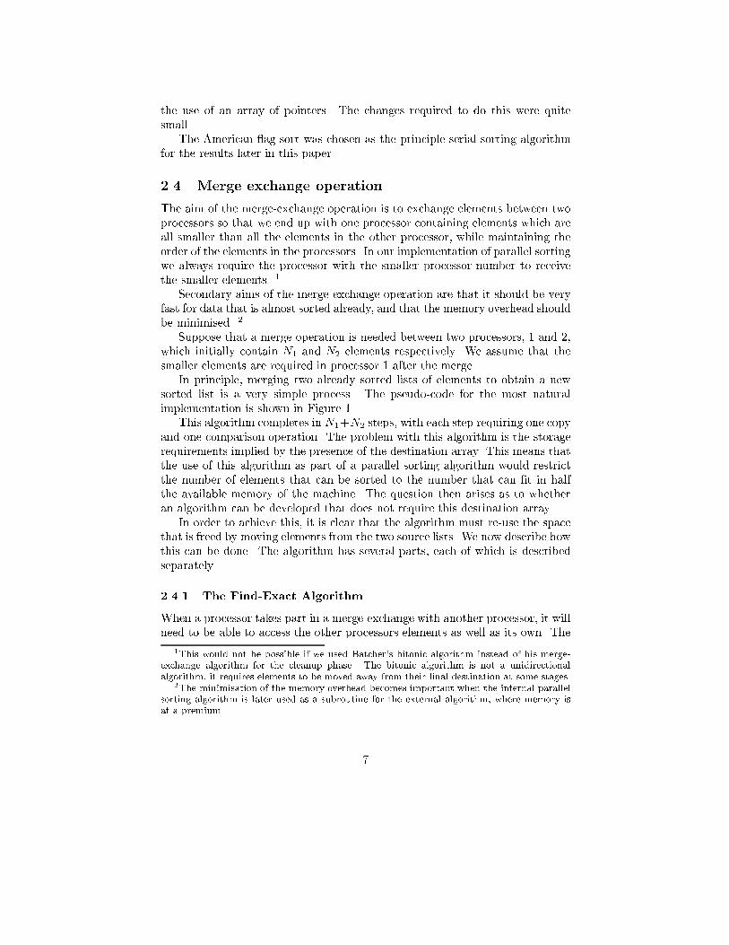
Figure 5: Partitioning with k = 3 and P = 6
into a number of slices, so that the number of elements in a slice does not exceedthe number that can be held in one processors memory.
A example of this partitioning is shown in Figure 5 for k = 3 and P = 6. Eachslice in the �gure is labeled with two sets of coordinates. One is its slice numberand the other is its (row,column) coordinates. The slice number uniquely de�nesthe slice whereas the (row,column) coordinates are shared between all slices ina grid square.
The snake like ordering of the slice numbers on the grid squares is essential tothe sorting process. Note that in the diagram the slices are labeled in snake-likefashion between the grid squares but are labeled left-right within a grid square.The ordering within a grid square is not essential to the sorting process but isfor convenience and code simplicity.
One di�culty in the partitioning is achieving some particular restrictions foron the numbers of slices, elements, processors and grid squares. The restrictionsare:
� The number of slices in a row or column must be less than or equal to thenumber of processors P
� The number of elements in a slice must be less than the amount of availablememory in a processor M 6
6Here and elsewhere in this paper we measure memory in units of elements, so one memoryunit is assumed to hold one element
16

These restrictions arise from the need to load all of a slice into a singleprocessor and the need to be able to load a complete row or column into thetotal internal memory. To achieve these requirements a iterative procedure isused which �rst estimates k and assigns slices then increases k if the restrictionsare not met.
The �le itself is mapped onto the slices in slice order. This means that eachslice represents a particular static region of the �le. Whenever a slice is loadedor saved the o�set into the �le is calculated from the slice number and the blockof elements at that o�set is loaded or saved to a single processors memory.
Note that the mapping of slices to �le position is static, but the mapping ofslices to processors is dynamic. This is discussed further in section 3.6.
3.4 Column and row sorting
The heart of the external sorting algorithm is the alternate column and rowsorting. To sort a row or column all slices with the required row or columnnumber are loaded into memory, with one slice per processor, then the internalsorting algorithm described previously is used to sort the row or column intoslice order.
The algorithm cycles through all columns on the grid, sorting each columnin turn, then cycles through each row in a similar fashion. This continues untilthe sort is complete. The detection of completion is discussed below.
The only change to the internal sorting algorithm previously presented is toeliminate the local sorting phase except the �rst time a slice is used. Once aslice has taken part in one row or column sort its elements will be internallysorted and thus will not need to be sorted in later passes.
3.5 Completion
An important part of the algorithm is the detection of completion of the sort.Although it would be possible to use the known properties of shear-sort toguarantee completion by just running the algorithm for dlog k + 1e passes, it ispossible to improve the average case enormously by looking for early completion.
Early completion detection is performed on a slice by slice basis, rather thanon the whole grid. Completion of the overall sorting algorithm is then de�nedto occur when all slices have completed.
The completion of a slice is detected by �rst augmenting each slice numberwith a copy of the highest and lowest element in the slice. The last processorto write the slice holds these elements.
At the end of each set of column or row sorts these sentinel elements are thengathered in one processor using a simple tree based gathering algorithm. Thisprocessor then check to see if the following two conditions are true to determineif the slice has completed
17

� the smallest element in the slice is larger than or equal to the largestelement in all preceding slices.
� the largest element in each slice is smaller than or equal to the smallestelement in each of the following slices
If these two conditions are true then all elements in the slice must be in theircorrect �nal positions. In this case the elements need never be read or writtenagain and the slice is marked as �nished. When all slices are marked as �nishedthe sort is complete. 7
3.6 Processor allocation
As slices are marked complete the number of slices in a row or column willdrop below the number of processors P . This means that if a strictly sequentialsorting of the rows or columns was made then processors would be left idle inrows or columns which have less than P slices remaining.
To take advantage of these additional processors the allocation of slices toprocessors is made dynamically. Thus while one row is being sorted additionalprocessors can begin the task of sorting the next row. Even if not enoughadditional processors are available to sort the next row a signi�cant savingcan be made because the data for the slices in the next row can be loaded,overlapping I/O with computation.
This dynamical allocation of processors can be done without additional com-munication costs because the result of the slice completion code is made avail-able to all processors through a broadcast from one cell. This means that allprocessors know what slices are not completed and can separately calculate theallocation of processors to slices.
3.7 Large k
The algorithm described above has a limit of k = P . Above this point theallocation of slices to processors becomes much trickier. The simplest way ofaddressing this problem is to allocate multiple grid squares to a processor. Amore complex alternative would be to sort recursively, so that rows and columnsare further subdivided into sections that can be handled by the available pro-cessors and memory.
A further problem that comes with very large values of k is that the worstcase of dlog k + 1e passes becomes a more signi�cant burden. To overcome thisproblem alternative grid sorting algorithms to shear-sort may be used whichwork well for much larger values of k. For example, reverse-sort[14] has a worst
7The determination of the two conditions can be accomplished in linear time by �rstcalculating the cumulative largest and cumulative smallest elements for each slice.
18

case of dlog log ke for large k. For smaller k, however, it has no advantage overshear-sort.
It is di�cult to properly investigate these large k parameter ranges as avail-able hardware (disk sizes) limits the available range of k to much less than Pfor current super-computer con�gurations. Values of k larger than P were notattempted in this paper.
3.8 Other partitionings
It may not be obvious from the above why a 2 dimensional partitioning was cho-sen. Other partitionings were considered as they lacked essential requirementsor were slower.
In particular many of the obvious one-dimensional sorting algorithms wouldrequire that either far fewer or far more than 1=k of the elements be in memoryat any one time. To have more than 1=k in memory would be impossible, andto have fewer would be ine�cient as the obviously valuable resource of memorywould be wasted.
Higher dimensional partitionings were also rejected after consideration. Onethat particularly appealed was a k dimensional hyper-cube, but it was simple toprove that its average case would be equal to the worst case of the 2 dimensionalpartitioning. It could not take advantage of the shortcuts which are so easy toproduce in the 2 dimensional case.
This is not to say that there isn't a better partitioning than the 2 dimensionalone proposed here. There may well be, but we haven't come up with one.
It should also be noted that if you were to choose k such that k =pN and
also assume that the serial sorting algorithm scales as N logN then one pass ofthe algorithm would take N logN time. The problem, however, is that k =
pN
would provide a much too �ne grained algorithm, which would su�er badly fromoverheads and latencies. The use of k = N=M is the best that can be done interms of the granularity of the algorithm.
19

4 Performance
The \proof of the pudding" is the speed. It is quite easy to create a parallelsorting algorithm that is asymptotically optimal, but it is much harder to createone which is fast over realistic data sizes.
In this section the performance of the above algorithms is examined for arange of data sizes and machine con�gurations.
4.1 The test environment
The principle test environment was a 128 processor Fujitsu AP1000 [5]. Thismachine contains 128 Sparc scalar processors connected on an 8 by 16 torus.Inter-processor communication is performed by hardware, using wormhole rout-ing. Each processor has 16Mb of local memory and all are connected to a hostworkstation via a relatively slow connection.
A 0.5GB SCSI disk is attached to 32 of the processors. Each disk is capableof a maximum transfer rate of 2MB/sec under ideal conditions. More typi-cal throughput for large transfers is 1.5MB/sec when the �lesystem overheadsare taken into account. The �lesystem used on the AP1000 was the HiDIOS�lesystem[15]. This gives a single �lesystem view across all the processors ratherthan each processor seeing only its own �les.
The AP1000 was programmed in C, using the MPI libraries for communica-tions. The code should be portable to other MPI implementations. The GNUC compiler version 2.6.3 was used.
The serial sorting routines were also tested on a Intel Pentium 90 PC runningLinux.
4.2 Serial sorting
As was pointed out earlier the algorithm used for the serial sorting componentsof the parallel sorting algorithm can have a very large impact on the overallperformance. It is important to choose a serial sorting algorithm which is wellsuited to the architecture of the target machine and to the distribution proper-ties of the data.
Figure 6 shows the speed in elements per second of sorting 64-bit integerson the Intel CPU as the number of elements to be sorted is varied. Two sortingalgorithms are shown, the top one is the American ag sort, modi�ed for inplaceinteger sorting. The bottom one is the GNU quicksort routine with inlinedcomparison function.
The graph clearly shows the speed advantage of the forward radix sortingused by the American ag sort. A speed di�erence of up to a factor or 5 isshown. The American ag sort also varies in speed much more across the rangetested. It is quite feasible that the quicksort will come close to the American
20

0
100000
200000
300000
400000
500000
600000
1000 10000 100000 1e+06
Ele
men
ts p
er s
econ
d
Number of elements
American Flag sort
Quicksort
Figure 6: Serial sorting 64 bit integers on a Pentium 90
ag sort for data sizes beyond what was tested here.8
Figure 7 shows the same graph for a AP1000 processor. In this case thespeed di�erence between the American ag sort and the quicksort is not nearlyas large. This re ects the di�erent processor architecture of the Sparc1+ andclearly demonstrates the importance of selecting a sorting algorithm that isappropriate for the target architecture.9
Figure 8 shows the speed of sorting 128 bit elements on the Intel CPU. It isinteresting to note that the speed has dropped by a factor much less than 2. Ifthe sorting algorithm was \ideal" then a factor of 2 decrease would be expectedas data movement costs would dominate. This suggests that there is room forfurther optimisation of these routines to reduce overheads.
Figure 9 shows the same graph for a AP1000 processor. Again the speedhas dropped by a factor much less than 2, and the di�erence between the twoalgorithms is not nearly as large as it is for the Intel CPU.
For the remainder of the testing in this paper the American ag sort is usedfor serial sorting components.
8The amount of memory available on the machine severely limits the range of data sizesthat can be tested
9It should be noted that the Sparc1+ CPUs in the AP1000 are quite old technology. Morerecent machines in the same line use SuperSparc CPUs which have much better performance
21

0
20000
40000
60000
80000
100000
120000
1000 10000 100000 1e+06
Ele
men
ts p
er s
econ
d
Number of elements
American flag sort
Quicksort
Figure 7: Serial sorting 64 bit integers on a AP1000 processor
0
100000
200000
300000
400000
500000
600000
1000 10000 100000 1e+06
Ele
men
ts p
er s
econ
d
Number of elements
American Flag sort
Quicksort
Figure 8: Serial sorting 128 bit integers on a Pentium 90
22

0
20000
40000
60000
80000
100000
120000
1000 10000 100000 1e+06
Ele
men
ts p
er s
econ
d
Number of elements
American flag sort
Quicksort
Figure 9: Serial sorting 128 bit integers on a AP1000 processor
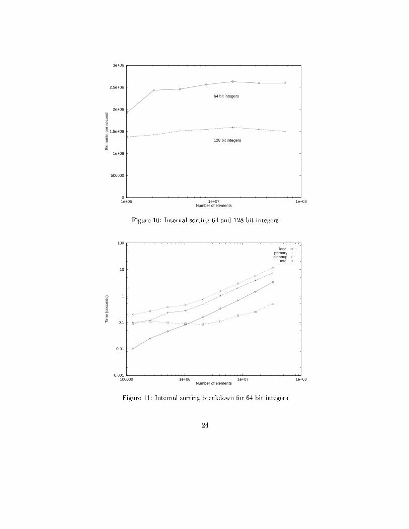
4.3 Internal parallel sorting
Figure 10 shows the speed of the internal sorting algorithm as the data size isvaried. The two graphs show the speed for 64 bit and 128 bit integers.
It is di�cult to extract from these results a accurate speedup (parallel e�-ciency) �gure. The problem is that the serial sorting algorithm results shownin Figure 7 and Figure 9 have no obviously good extrapolation. If, however, weuse a very simple extrapolation then we might estimate the serial sorting ratefor large data sizes would be 50000 elements per second for 64 bit integers and40000 elements per second for 128 bit integers.
Given these estimates we get an approximate speedup of 50 and 38 respec-tively. This is much less than the ideal 128 times speedup for this machine.The reason for this less than ideal speedup comes from the extremely optimisednature of the american ag sort. In a previous paper[11] a much higher speedupwas found for the same algorithm when using the GNU quicksort algorithm forserial sorting.
A breakdown by time of the internal sorting algorithm is shown in Figure 11for 64 bit integers and Figure 12 for 128 bit integers. These graphs show thatthe time is dominated by the primary merge phase of the algorithm.
The cleanup phase becomes insigni�cant as the data size rises, showing thatthe primary merge is doing its job of almost sorting the data.
23
0
500000
1e+06
1.5e+06
2e+06
2.5e+06
3e+06
1e+06 1e+07 1e+08
Ele
men
ts p
er s
econ
d
Number of elements
64 bit integers
128 bit integers
Figure 10: Internal sorting 64 and 128 bit integers
0.001
0.01
0.1
1
10
100
100000 1e+06 1e+07 1e+08
Tim
e (s
econ
ds)
Number of elements
localprimarycleanup
total
Figure 11: Internal sorting breakdown for 64 bit integers
24

0.01
0.1
1
10
100
100000 1e+06 1e+07 1e+08
Tim
e (s
econ
ds)
Number of elements
localprimarycleanup
total
Figure 12: Internal sorting breakdown for 128 bit integers
4.4 External sorting
The problem with measuring the speed of external sorting is �nding enough diskspace. The AP1000 has 2GB of internal memory, which means you need to sortconsiderably more than 2GB of data to reach reasonable values of k. Unfortu-nately only 10GB (of a possible 16GB) is allocated to the HiDIOS �lesystem,so a k above 5 is not really possible. In practice a k of above 2 is di�cult toachieve as the disks are invariably quite full.
To overcome this problem the following experiments limit the amount of ramavailable to the program to much less than the full 2GB. This allows a muchwider range of external sorting parameters to be explored.
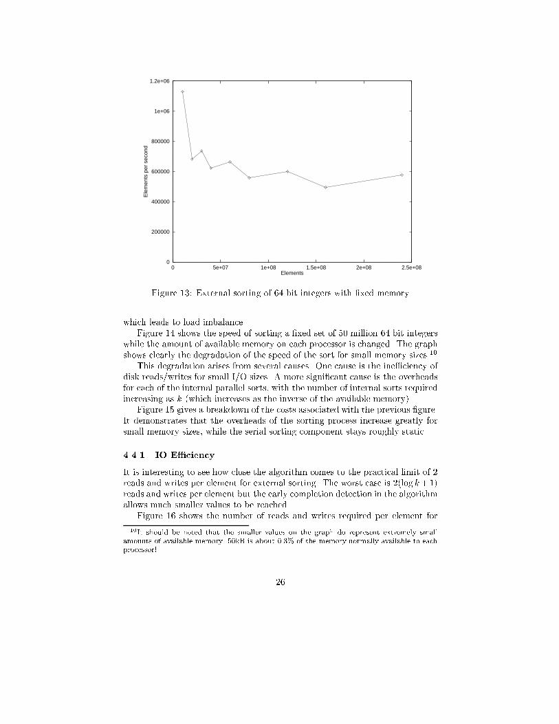
Figure 13 shows the speed in elements per second of a external sort wherethe available memory per processor has been �xed at 1MB (excluding operatingsystem overheads). This means that k increases with the number of elements tobe sorted. The left most point on the graph is in fact an internal sort as thereis su�cient memory available for k = 1, meaning the data can �t in internalmemory. This graph includes the I/O overhead of loading and saving the data,which is why the internal point is considerably slower than the previous internalresults.
The alternate high-low structure of the graph is due to the number of ele-ments not being close to a multiple of k2 for the lower results. This means thatmany grid squares on the k�k grid are a long way from being completely �lled,
25
0
200000
400000
600000
800000
1e+06
1.2e+06
0 5e+07 1e+08 1.5e+08 2e+08 2.5e+08
Ele
men
ts p
er s
econ
d
Elements
Figure 13: External sorting of 64 bit integers with �xed memory
which leads to load imbalance.Figure 14 shows the speed of sorting a �xed set of 50 million 64 bit integers
while the amount of available memory on each processor is changed. The graphshows clearly the degradation of the speed of the sort for small memory sizes 10
This degradation arises from several causes. One cause is the ine�ciency ofdisk reads/writes for small I/O sizes. A more signi�cant cause is the overheadsfor each of the internal parallel sorts, with the number of internal sorts requiredincreasing as k (which increases as the inverse of the available memory).
Figure 15 gives a breakdown of the costs associated with the previous �gure.It demonstrates that the overheads of the sorting process increase greatly forsmall memory sizes, while the serial sorting component stays roughly static.
4.4.1 IO E�ciency
It is interesting to see how close the algorithm comes to the practical limit of 2reads and writes per element for external sorting. The worst case is 2(log k+1)reads and writes per element but the early completion detection in the algorithmallows much smaller values to be reached.
Figure 16 shows the number of reads and writes required per element for
10It should be noted that the smaller values on the graph do represent extremely smallamounts of available memory. 50kB is about 0.3% of the memory normally available to eachprocessor!
26

0
200000
400000
600000
800000
1e+06
10 100 1000 10000
Ele
men
ts p
er s
econ
d
Memory per processor (kB)
Figure 14: External sorting of 50 million 64 bit integers with varying amountsof available memory
0
20
40
60
80
100
10 100 1000 10000
IOCleanup
Local sortPrimary
Figure 15: Breakdown of cost of external sorting as amount of available memoryvaries
27

2
2.05
2.1
2.15
2.2
2.25
1 10 100
Rea
ds a
nd W
rites
per
ele
men
t
k
Figure 16: Number of reads and writes per element for a range of k values
random 64 bit integers. Note the narrow y scale. The graph shows that thealgorithm achieves close to the ideal 2 reads and writes per element over a widerange of k, with a slight increase for larger k. This demonstrates that the earlycompletion detection part of the algorithm is functioning well.
4.4.2 Worst case
An important property of a sorting algorithm is the worst case performance.Ideally the worst case is not much worse than the average case, but this is hardto achieve.
For the internal sorting the worst case is achieved when the data has adistribution which gives the worst case for the American ag sort. This meansthe distribution must be such that all bytes are required to sort the data, sothat the early completion detection cannot be used. The worst histogram forthe American ag sort is one which covers a wide range of byte values, as ituses an optimisation which relies on the byte values covering less than the fullrange. This means the worst case is when each byte of the data is randomly 0or 255 with equal probability.
A experiment with 10 million 64 bit elements and a k of 1 (internal sorting)gave a slowdown for the worst case compared to random data of about a factorof 2.
The worst case for the external sorting algorithm is when the data starts
28
out sorted by the column number that is assigned after the partitioning stage.This will mean that the initial column sort will not achieve anything. The worstcase of log k+1 passes can then be achieved. Additionally the data distributionrequired for the worst case of the internal sorting algorithm should be used.
A experiment with 10 million 64 bit elements and a k of 7 gave a slowdownfor the worst case compared to random data of about a factor of 4.
29

5 Conclusions
This paper has presented algorithms for internal and external parallel integersorting. The algorithms have a high parallel e�ciency and are well suited tomassively parallel machines such as the AP1000.
The in-core sorting experiments demonstrated a sorting speed of over 2 mil-lion elements per second for sorting more than 1 million 64 bit integers on a128 processor AP1000. For 128 bit integers 1.5 million elements per second wasachieved for more than 50 million elements.
The secondary memory sorting experiments demonstrated a speed of 7 hun-dred thousand elements per second for 64 bit integers with a limited amountof memory available per processor. The strong dependence on the amount ofavailable memory was also demonstrated.
Parameters Millions of elements per second
in core, 64 bit, 1M elements 2in core, 128 bit, 50M elements 1.5external, 64 bit, 50M elements 0.7
There is probably still considerable room for improvement in the detailedimplementation of the algorithms, in particular the reduction of overheads as-sociated with each internal sort in the external sorting algorithm. A much �nergrained pro�ling will be needed to identify the bottlenecks.
6 Source code
The full source code (using C and MPI) is available from the authors. It shouldbe easily portable to other systems which support the MPI interface. It consistsof a bit under 3000 lines of code.
The main program in main.c is merely a convenient test harness. It canbe used to generate and sort data under a variety of conditions, controlledby command line options. For a real application it is likely that the code inpar sort.c would be used as the basis for a library routine.
6.1 Using the test program
The test program can generate and sort data under a wide variety of conditions.On the AP1000 it would be used like this:
mpirun -nohost capsort [options] infile outfile
If the input and output �les are the same then the �le is sorted in place. Iftwo �les are speci�ed then the input �le is �rst copied to the output �le thenthe data is again sorted in place in the output �le.
30

There are a large number of options that can be applied. Here is a briefsummary:
-p causes the data to be printed to standard output before and after sorting.This is useful for debugging.
-v causes the main program to verify the sort by calling qsort() within oneprocessor and comparing the result. This will only work if the data �ts inone processors memory and the input and output �les are not the same�le.
-D causes the main program to delete the �le after sorting. This is useful forcleaning up after a test run.
-l NUM causes the main program to loop, calling the sort routine NUM times.At the end of each loop the parameters are changed. How they are changedis currently controlled by code changes in the main loop. This is usefulfor generating graphs.
-w causes the code to try to produce the worst case.
-g NUM causes the main program to generate NUM items of random data inthe input �le.
-s NUM seeds the random number generator with NUM.
-m NUM sets the memory limit per processor to NUM kB.
More detailed information on running the program can be obtained by read-ing the source code.
31

References
[1] M. Ajtai, J. Kolmos and E. Szermeredi, \Sorting in c logn parallel steps",Combinatorica 3, 1983, 1-19.
[2] S. G. Akl, Parallel Sorting Algorithms, Academic Press, Toronto, 1985.
[3] G. E. Blelloch, C. E. Leiserson, B. M. Maggs, C. G. Plaxton, S. J. Smith andM. Zagha, \A comparison of sorting algorithms for the Connection MachineCM-2", Proc. Symposium on Parallel Algorithms and Architectures, HiltonHead, South Carolina, July 1991.
[4] G. C. Fox, M. A. Johnson, G. A. Lyzenga, S. W. Otto, J. K. Salmonand D. W. Walker, Solving Problems on Concurrent Processors, Volume 1,Prentice-Hall, Englewood Cli�s, New Jersey, 1988.
[5] H. Ishihata, T. Horie, S. Inano, T. Shimizu and S. Kato, \CAP-II Ar-chitecture", Proceedings of the First Fujitsu-ANU CAP Workshop, FujitsuResearch Laboratories, Kawasaki, Japan, November 1990.
[6] D. E. Knuth, The Art of Computer Programming, Volume 3: Sorting and
Searching (second edition), Addison-Wesley, Menlo Park, 1981, 112-113.
[7] ibid, solution to problem 5.3.4 (38).
[8] L. Natvig, \Logarithmic Time Cost Optimal Parallel Sorting is Not YetFast in Practice!", Proc Supercomputing 90, IEEE Press, 1990, 486-494.
[9] H. H. Reif and L. G. Valiant, \A logarithmic time sort for linear size net-works", J. ACM 34, 1987, 60-76.
[10] K. Thearling and S. Smith, \An Improved Supercomputing Sorting Bench-mark", Proc Supercomputing 92, IEEE Press, 1992, 14-19.
[11] A. Tridgell and R. P. Brent, An Implementation of a General-Purpose Par-
allel Sorting Algorithm, Report TR-CS-93-01, Computer Sciences Labora-tory, Australian National University, February 1993, 24 pp.
[12] D. McIlroy, P. McIlroy and K. Bosti, Engineering radix sort Computingsystems, vol 6, no 1, winter 1993
[13] Scherson, Sen and Shamir, Shear sort: A True Two Dimensional Sorting
Technique for VLSI Networks, Tech report, Dept of Electrical and Com-puter Engineering, University of California, 1985
[14] C. P. Schnorr, An optimal Sorting Algorithm For Mesh Connected Com-
puters, Proc. ACM Synmposium on the Theory of Computation, 1986
[15] A. Tridgell and D. Walsh , The HiDIOS Filesystem, Proceedings of the
Fujitsu CAP Workshop, Imperial College, London, October 1995.
32