Embed Size (px)
Citation preview
PARALLEL IMPLEMENTATION OF A RAY TRACER
FOR UNDERWATER SOUND WAVES USING THE
CUDA LIBRARIES:
DESCRIPTION AND APPLICATION TO THE SIMULATION OF
UNDERWATER NETWORKS
RELATORE: Ch.mo Prof. Michele Zorzi
CORRELATORE: Dott. Paolo Casari
LAUREANDO: Matteo Lazzarin
A.A. 2011-2012

UNIVERSITA DEGLI STUDI DI PADOVA
DIPARTIMENTO DI INGEGNERIA DELL’INFORMAZIONE
TESI DI LAUREA
PARALLEL IMPLEMENTATION OF A RAY
TRACER FOR UNDERWATER SOUND
WAVES USING THE CUDA LIBRARIES:
DESCRIPTION AND APPLICATION TO THE SIMULATION OF
UNDERWATER NETWORKS
RELATORE: Ch.mo Prof. Michele Zorzi
CORRELATORE: Dott. Paolo Casari
LAUREANDO: Matteo Lazzarin
Padova, April 24, 2012

2

Abstract
One of the most time-consuming parts of the simulation of underwater networks
is the realistic simulation of underwater sound propagation. Some well-known
software tools used for networks simulations to date employ ray tracing to sim-
ulate sound propagation. This gives rise to high computational complexity, and
may require very long time to complete a simulation. In this thesis we present a
faster tool able to simulate an underwater sound channel. The software is based
on ray tracing and is based on the CUDA architecture, the general-purpose par-
allel computing architecture that uses the parallel computing engine in NVIDIA
GPUs to efficiently solve complex computational problems. Following the CUDA
programming model guideline, a ray tracer has been developed where the trajec-
tory computation is performed in a CUDA-enabled parallel way, obtaining a ray
tracer implementation that completes faster than the widely use single-thread
Bellhop software.
3

Sommario
Una delle parti piu dispendiose sotto l’aspetto del tempo impiegato nella simu-
lazione di reti subacquee e la simulazione della propagazione sonora. Alcuni dei
piu noti software di settore per svolgere le simulazioni utilizzano il metodo di ray
tracing. L’elevata complessita computazionale puo far si che le simulazioni ne-
cessitino di molto tempo per essere effettuate. In questa si presenta un software
in grado di velocizzare tali simulazioni. Il programma, coadiuvato dalla potenza
di calcolo offerta dall’architettura parallela CUDA, implementa un ray tracer in
grado di calcolare le traiettorie in modo parallelo. Cio ha permesso di ottenere
un simulatore con prestazioni decisamente migliori rispetto al ben noto software
ad implementazione classica Bellhop.
4


Contents
1 The CUDA Architecture 4
1.1 Introduction . . . . . . . . . . . . . . . . . . . . . . . . . . . . . . 4
1.1.1 From Graphics Processing To General-Purpose Parallel Com-
puting . . . . . . . . . . . . . . . . . . . . . . . . . . . . . 4
1.1.2 A General Purpose Parallel Computing Architecture Named
CUDA . . . . . . . . . . . . . . . . . . . . . . . . . . . . . 7
1.1.3 A scalable Programming Model . . . . . . . . . . . . . . . 7
1.2 Heterogeneous Computing . . . . . . . . . . . . . . . . . . . . . . 9
1.2.1 Host vs. Device . . . . . . . . . . . . . . . . . . . . . . . . 9
1.2.2 What runs on a CUDA enabled device . . . . . . . . . . . 10
1.2.3 Scaling . . . . . . . . . . . . . . . . . . . . . . . . . . . . . 12
1.2.4 Understanding scaling . . . . . . . . . . . . . . . . . . . . 14
1.2.5 Getting the right answer . . . . . . . . . . . . . . . . . . . 15
1.3 Hardware Implementation . . . . . . . . . . . . . . . . . . . . . . 16
1.3.1 Single-Instruction Multiple-Thread Architecture . . . . . . 16
1.3.2 Control Flow . . . . . . . . . . . . . . . . . . . . . . . . . 19
1.4 The Kernels . . . . . . . . . . . . . . . . . . . . . . . . . . . . . . 20
ii

1.5 The Threads . . . . . . . . . . . . . . . . . . . . . . . . . . . . . . 21
1.5.1 Definition . . . . . . . . . . . . . . . . . . . . . . . . . . . 21
1.5.2 CUDA Threads . . . . . . . . . . . . . . . . . . . . . . . . 21
1.6 Memory Hierarchy . . . . . . . . . . . . . . . . . . . . . . . . . . 22
1.6.1 Memory Bandwidth . . . . . . . . . . . . . . . . . . . . . . 22
1.6.2 Device Memory Spaces . . . . . . . . . . . . . . . . . . . . 25
1.6.3 Registers . . . . . . . . . . . . . . . . . . . . . . . . . . . . 27
1.6.4 Shared Memory . . . . . . . . . . . . . . . . . . . . . . . . 28
1.6.5 Global Memory . . . . . . . . . . . . . . . . . . . . . . . . 30
1.6.6 Local Memory . . . . . . . . . . . . . . . . . . . . . . . . . 35
1.6.7 Texture Memory . . . . . . . . . . . . . . . . . . . . . . . 35
1.6.8 Constant Memory . . . . . . . . . . . . . . . . . . . . . . . 36
1.7 More Practical Aspects . . . . . . . . . . . . . . . . . . . . . . . . 37
1.7.1 The compiler: NVCC . . . . . . . . . . . . . . . . . . . . . 38
2 Ocean Acoustics 41
2.1 The Undersea Environment . . . . . . . . . . . . . . . . . . . . . 41
2.2 Sound propagation in the ocean . . . . . . . . . . . . . . . . . . . 44
2.2.1 Deep water propagation . . . . . . . . . . . . . . . . . . . 48
2.2.2 Arctic Propagation . . . . . . . . . . . . . . . . . . . . . . 54
2.2.3 Shallow Water Propagation . . . . . . . . . . . . . . . . . 54
2.3 Sound attenuation in sea water . . . . . . . . . . . . . . . . . . . 57
2.4 Bottom Interaction . . . . . . . . . . . . . . . . . . . . . . . . . . 60
iii

3 Implementation Of A Ray Tracer for Underwater Sound Propa-
gation Modeling Using CUDA 63
3.1 Introductory material . . . . . . . . . . . . . . . . . . . . . . . . . 63
3.1.1 A Brief Mathematical Introduction . . . . . . . . . . . . . 64
3.1.2 Stratified media . . . . . . . . . . . . . . . . . . . . . . . . 68
3.1.3 Path in the whole stratified medium . . . . . . . . . . . . 69
3.2 CUDA Algorithm . . . . . . . . . . . . . . . . . . . . . . . . . . . 72
3.3 Performance . . . . . . . . . . . . . . . . . . . . . . . . . . . . . . 80
3.4 Pressure computation . . . . . . . . . . . . . . . . . . . . . . . . . 85
Bibliography 91
iv


Introduction
This thesis presents the parallel implementation of a ray tracer algorithm for
the simulation of underwater sound propagation. Ray tracing is a widely used
procedure that allows to solve the propagation equations for a wave on a inho-
mogeneous medium. In ray tracing, the problem is approached by simulating the
propagation of narrow beams called rays, where trajectory is pointwise orthogo-
nal to the wave front.
The propagation of a ray is completely independent of the propagation of each
other rays, hence the method can take advantages of an implementation on a par-
allel architecture, substantially improving the the performance of the algorithm.
The parallel architecture we chose for the tracer implementation is the modern
NVIDIA CUDA architecture, a general-purpose parallel computing architecture
with a new parallel programming model and instruction set that uses the paral-
lel compute engine in NVIDIA GPUs to solve complex computational problems
efficiently.
Following the CUDA programing model guideline, it has been developed a ray
tracer on which the trajectory computation in made in a parallel way. The
parallelization takes place both across the rays and inside every ray. By this
design, the tracer takes advantage from the hardware acceleration offered by
CUDA throughout the execution.
The developed software has been compared with the exiting serial program Bell-
hop on different systems, both entry-level and high-end architectures.
The results show that the benefit achieved using the parallel approach is signif-
icant: the simulation times reached by the CUDA implementation are several
time smaller than those obtained with the Bellhop.
1

The network simulations performed using the CUDA implementation of the ray
tracer would achieve a significant speedup, in turn.
2


Chapter 1
The CUDA Architecture
This part summarize the key aspects of the CUDA architecture. It is based on
[2, 3, 5, 8], where the contents of this part are treated in more detail.
1.1 Introduction
1.1.1 From Graphics Processing To General-Purpose Par-
allel Computing
Today’s demand for realtime, high-definition 3D graphics, has forced graphic card
vendors into a continuous run for increasing devices performance. The modern
programmable Graphic Processor Units (GPUs) have evolved into highly parallel,
multi threaded processors with huge computational power and very high memory
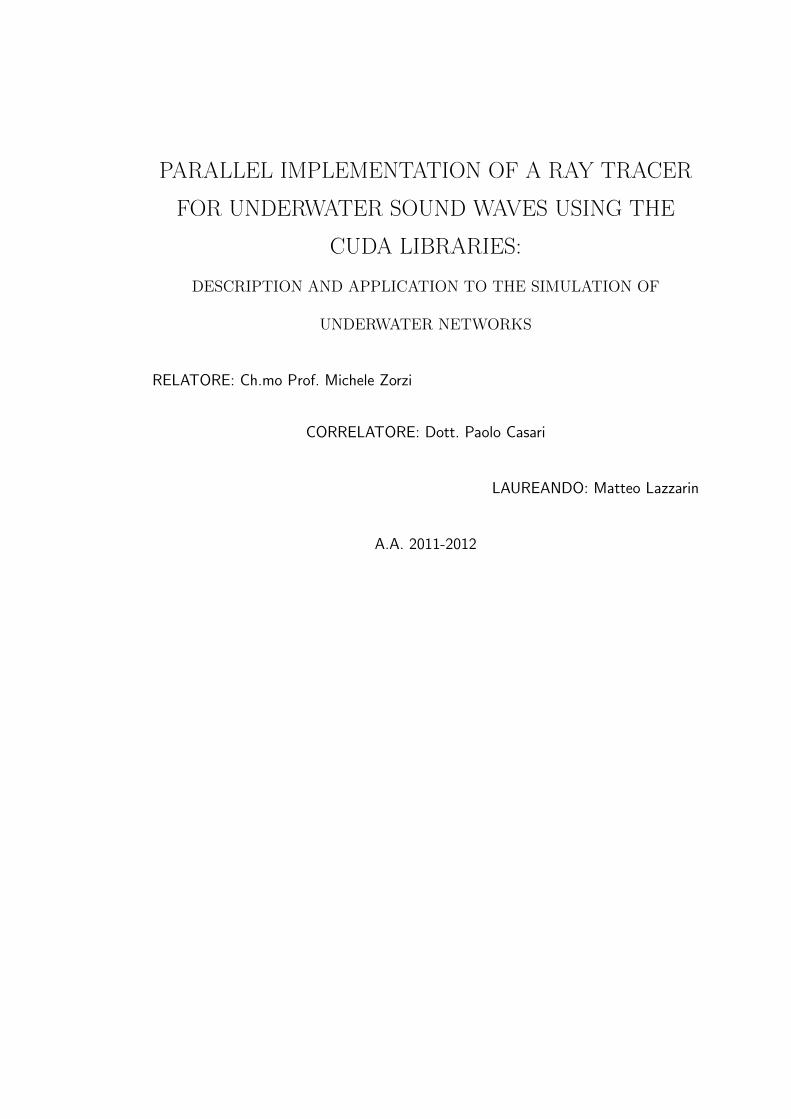
bandwidth, as illustrated in 1.1 and 1.2.
4
Figure 1.1: CPUs and GPUs performance growth on the last ten-years period
Figure 1.2: CPUs and GPUs performance growth on the last ten-years period
The reason behind the discrepancy in the theoretical number of floating-point
operations per second observed between the CPU and the GPU (in figure 1.1 is
that the GPU is specialized for the intensive, highly parallel computation that
graphics rendering requires, and is therefore designed such that more transistors
are devoted to data processing rather than data caching and flow control, as
5

schematically illustrated by figure 1.3.
More specifically, the GPU is especially designed to address as efficiently as pos-
sible problems that can be configured as data parallel computations. The same
program is executed on many data elements in parallel, with high arithmetic in-
tensity. Because the same program is executed for each data element, there is
no requirement for sophisticated flow control techniques. Moreover, because it is
executed on many data elements and has high arithmetic intensity, the memory
access latency can be hidden with calculations instead of big data caches.
Data-parallel processing maps data elements to parallel processing threads. Many
applications that process large data sets can use a data-parallel programming
model to speed up the computations.
As for instance in 3-D rendering, large sets of pixels and vertices are mapped
to parallel threads, similarly image and media processing applications (such as
post-processing of rendered images, video encoding and decoding, image scal-
ing, stereo vision, and pattern recognition) can map image blocks and pixels to
parallel processing threads. In fact, many algorithms outside the field of image
rendering and processing are accelerated by data-parallel processing, from general
signal processing or physics simulation to computational finance or computational
biology.
Figure 1.3: Differences between CPU and GPU architecture
6

1.1.2 A General Purpose Parallel Computing Architec-
ture Named CUDA
In November 2006, NVIDIA corporation has introduced a new architecture named
CUDA. It is essentially a general-purpose parallel computing architecture with
a new parallel programming model and instruction set that uses the parallel
compute engine in NVIDIA GPUs to solve complex computational problems more
efficiently that with a CPU.
CUDA comes with a software development kit that allows programmers to use
C/C++ as a high-level programming language. Other languages or application
programming interfaces are also supported, such as CUDA FORTRAN, OpenCL,
and DirectCompute.
1.1.3 A scalable Programming Model
The advent of multi-core CPUs and many-core GPUs means that mainstream
processor chips can be handled as a parallel system from all points of view. Fur-
thermore, their parallelism continues to scale with Moore’s law, and so does their
performance.
The challenge the developer have to face is to build application software that
transparently scales its parallelism to leverage on the increasing number of pro-
cessor cores, as much as 3-D graphics applications transparently scale their par-
allelism to many-core GPUs with a widely varying number of cores.
The CUDA parallel programming model is designed to overcome this challenge, by
maintaining a low learning curve for programmers already familiar with standard
programming languages such as C/C++ or FORTRAN.
One of the programmers goals is to partition the problem into coarse sub-problems
that can be solved independently in parallel by blocks of threads, and each sub-
problem into finer pieces that can be solved cooperatively in parallel by all threads
within each block.
This decomposition preserves language expressivity by allowing threads to coop-
7

erate when solving each sub-problem, and at the same time it enables automatic
scalability. Each block of threads can be scheduled on any of the available pro-
cessor cores, in any order, concurrently or sequentially, so that a compiled CUDA
program can be run on any number of processor cores as illustrated by Figure
1.4, where only the runtime system needs to know the physical processor count.
This scalable programming model allows the CUDA architecture to span a wide
market range by simply scaling the number of processors and memory partitions:
from the high-performance GeForce GPUs and professional Quadro and Tesla
computing products to a variety of inexpensive, mainstream GeForce GPUs. Us-
ing the recent Tegra architecture,the mobile devices could also benefit from this
approach in the future.
Figure 1.4: A multithreaded program is partitioned into blocks of threads that
can be run independent of each other, so that a GPU with more cores will auto-
matically execute the program in less time than a GPU with fewer cores
8

1.2 Heterogeneous Computing
CUDA programming involves running code on two different platforms concur-
rently: a host system with one or more CPUs and one or more CUDA-enabled
NVIDIA GPU devices. NVIDIA GPUs are generally associated only with graphic
devices, however they are also powerful arithmetic engines, capable of running
thousands of lightweight threads in parallel. This capability makes them handy
to compute a parallel algorithm. However, the device is based on a distinctly
different design than the host system, and it is important to understand those
differences and how they influence the performance of CUDA applications, in
order to use CUDA at its best.
1.2.1 Host vs. Device
In the following list the primary differences are described between the host and
the CUDA device.
Threading Resources
Execution pipelines on host systems can support a limited number of con-
current threads. For example, high-end servers can have four hex-core
processors, and can therefore run 24 threads concurrently (or 48, if Hy-
perThreading is supported.). For comparison, the smallest executable unit
of parallelism on a CUDA device comprises 32 threads (termed a warp of
threads). Nowadays NVIDIA GPUs can support up to 1536 active threads
concurrently per many-core processor. This means that on a GPUs with 16
processor there can be more than 24,000 active threads alive at the same
time.
Threads
Threads on a CPU are generally heavyweight entities. The operating system
must swap threads on and off CPU execution channels to provide multi-
threading capability. Context switches (when two threads are swapped) are
typically slow and expensive. By comparison, GPU threads are extremely
lightweight. In a typical system, thousands of threads are queued up (in
9

warps of 32 threads each). If the GPU must wait on one warp of threads,
it simply begins executing work on another. Because separate registers are
allocated to all active threads, no swapping of registers or other state need
occur when switching among GPU threads. These resources are allocated
to each thread until its execution is completed. In summary, CPU cores are
designed to minimize latency for one or two threads at a time each, whereas
GPUs are designed to handle a large number of concurrent, lightweight
threads in order to maximize throughput.
It is useful to point out that the program flow control system, on a CPU,
is much more sophisticated than in a GPU. This, sometimes, can be a big
limitation, as we will see later.
RAM
The host system and the device each have their own distinct attached phys-
ical memory. The host and device memory communicate through the PCI
Express (PCIe) bus. The items in the host memory can be moved to the
device memory and using back the PCIe bus.
These above are the primary hardware differences between CPU hosts and GPU
devices with respect to parallel programming. The applications written with
these differences in mind can treat the host and device together as an integrated,
heterogeneous system where each processing unit is employed to do the kind of
work it does best: sequential work on the host, and parallel work on the device.
1.2.2 What runs on a CUDA enabled device
The following issues should be considered when determining what parts of an
application should run on a CUDA-enabled device and what parts should not:
• The GPU device is designed to address parallel computations, that can
involve numerous data elements simultaneously. This typically involves
arithmetic operations on large data sets (such as matrices) where the same
operation can be performed on thousands, if not millions, of elements at the
same time. This is a requirement for good performance on CUDA: the soft-
10

ware must use a large number (generally thousands, or tens of thousands)
of concurrent threads.
The support for running numerous threads in parallel derives from the
CUDA architecture’s use of a lightweight threading model, as described
above.
• In order to achieve the best performance, there should be some coherence in
memory access by adjacent threads running on the device. Certain memory
access patterns enable the hardware to coalesce groups of reads or writes
of multiple data items into one operation. Data that cannot be laid out so
as to enable coalescing, or that does not have enough locality to use the
global memory cache or on the texture cache effectively, will tend to see
minor speedups when used in CUDA computations.
• To use CUDA, the data values required by the calculations must transferred
from the host to the device using the PCI Express (PCIe) bus, and then
back to the host. These transfers are costly in terms of performance and
their occurance should be minimum. The following two rules of thumb help
to evaluate whether CUDA devices are properly used:
– The complexity of operations should justify the cost of mov-
ing data to and from the device
Code that transfers data for brief use by a small number of threads
will exhibit little or no performance benefit. The ideal scenario is one
in which many threads perform a substantial amount of work.
For example it is useful to analyze the case of a sum of matrices. In
this case, transferring two matrices from the host to the device and
then transferring the results back to the host will not achieve a large
performance benefit.
The issue here is the number of operations performed per data ele-
ment transferred. For the preceding procedure, assuming matrices of
size N × N , there are N2 operations (additions) and 3N2 elements
transferred, so the ratio of operations to elements transferred is 1:3 or
O(1).
11

Performance benefits can be more readily achieved when this ratio is
higher. For example, the multiplication of the same matrices requires
N3 operations (multiply-add), so the ratio of the number of operations
to the number of elements transferred is O(N), hence the larger the
matrix the greater the performance benefit. The types of operations
are an additional factor to take into account, as additions have different
complexity profiles than, for example, trigonometric functions.
To summarize, it is important to include the overhead of transferring
data to and from the device in order to determine if operations should
be performed on the host or on the device.
– Data should be kept on the device as long as possible.
The number of data transfers should be minimized. The programs that
run multiple kernels, ( program functions executed by CUDA, they
will be described deeply in 1.4 ) on the same data should favor leaving
the data on the device between kernel calls, rather than transferring
intermediate results to the host and then sending them back to the
device for subsequent calculations. In the previous example, if the two
matrices had already been added on the device as a result of some
previous calculation, or if the results of the addition are required in
some subsequent calculation, the matrix addition should be performed
on the device. This approach should be used even if one of the steps
in a sequence of calculations could be performed faster on the host.
Even a relatively slow kernel may be advantageous if it avoids one or
more PCIe transfers.
1.2.3 Scaling
In our case the term how well a program scales refer to the amount of benefit
that it will achieve by increasing the size of the computation.
By understanding how an application can scale is useful to identify bounds that
lead us to choose the parallelization strategy best suited for a specific problem.
The benefit an application will achieve by running on CUDA depends entirely on
the extent to which it can be parallelized. The code that cannot be sufficiently
12

parallelized should be run on the host. That because the cost of supplementary
memory transactions needed by a CUDA kernel could overcome benefits.
Strong Scaling
Strong scaling measures how the time to complete a computation decreases as
more processors are added to a system for a fixed overall problem size.
An application that exhibits a linear scaling has a speedup proportional to the
number of processors added into the system.
Strong scaling is usually equated with Amdahl’s Law. Amdahl’s Law specifies
the upper bound of the speedup which an application can get by parallelizing
part of its code. Essentially the maximum speedup S that a program can reach
is:
S =1
(1− P ) + PN
where
• P is the fraction of the total serial execution time spent by the part of the
code that can be parallelized .
• N is is the number of processors available to run the part of code parallelized.
Hence, the larger N is i.e. the greater the number of available processors, the
smaller the fraction PN
becomes. When N is sufficiently large, the fraction above
tends to zero:
limN→∞
1
(1− P )− PN
=1
(1− P )= S
For instance, if three quarters of some code can be parallelized, the maximum
speedup, that can be achieved is
Smax =1
1− 34
= 4
In practical cases, most applications do not exhibit a perfect linear strong scaling.
Anyway, the key message of this section is that the larger the parallelized portion
13

of code is, the greater speedup the parallel code exhibits.
Conversely, if P is a small number (meaning that the application is not sufficiently
parallelizable) increasing the number of processors N does little to improve perfor-
mance. Hence, to get the largest speedup for a fixed problem size it is necessary
to spend same initial effort on increasing P, maximizing the amount of code that
can be parallelized.
Weak Scaling
Weak scaling is a measure of how the time to complete a computational changes
as more processors are added to a system with a fixed problem size per processor;
i.e. , both the overall problem size and the number of processors increase.
Weak scaling is often equated with Gustafson’s Law, which states that, in prac-
tice, the problem size scales with the number of processors. Because of this, the
maximum speedup of a program will be:
S = N + (1− P )(1−N)
where, as for the strong scaling
• P is the fraction of the total serial execution time spent by the part of code
that can be parallelized.
• N is the number of processors available to run the parallel parts of code.
1.2.4 Understanding scaling
To understand which kind of scaling is most applicable to an application is an
important part the programmer should take into account in order to estimate
speedup.
Having understood the application profile, the developer should understand how
the problem size would change if the computational performance change and then
apply either Amdahl’s or Gustafson’s Law to determine an upper bound for the
speedup
14

1.2.5 Getting the right answer
Obtaining the right answer is clearly the principal goal of any computation.
On parallel systems, usually, it is possible to run into challenges typically not
found in traditional serial-oriented programming. These include threading is-
sues, unexpected values due to the way floating-point values are computed, and
challenges arising from differences in the way CPU and GPU processors operate.
Numerical Accuracy
A key aspect of correctness verification for parallel modifications to any exist-
ing program is to establish some mechanism whereby previous reference outputs
obtained from representative inputs can be compared to the results of parallel
computations.
After each change is made, one should ensure that the results match. Some will
expect bitwise identical results, which is not always possible, especially where
floating-point arithmetic is involved.
In general the major problems arise when floating-point computations are in-
volved.
A typical issue is represented by the mixed use of double and single precision
floating point values. Because of their different precision, the results are affected
by rounding and thus they have to be analyzed considering a certain tolerance.
Another frequent issue (very simple to understand but not trivial at all) regards
the fact that floating-point math is not associative. Each floating-point arith-
metic operation involves a certain amount of rounding. Consequently, the order
in which arithmetic operations are performed is important. If A, B, and C are
floating-point values, (A+B) +C is not guaranteed to equal A+ (B +C) ( and
in general it is not) as it is in symbolic math.
When the computation is made parallel, it potentially change the order of opera-
tions and therefore, the parallel results might not match the serial computation.
This limitation is not specific of CUDA, but an inherent issue of parallel compu-
tation on floating-point values.
15
1.3 Hardware Implementation
The CUDA architecture is built around a scalable array of multithreaded Stream-
ing Multiprocessors (SMs).
When a CUDA program on the host CPU invokes a kernel grid, the blocks of the
grid are enumerated and distributed to multiprocessors with available execution
capacity as previously shown in figure 1.4.
The threads of a thread block are executed concurrently on one multiprocessor,
and multiple thread blocks can be executed concurrently on one multiprocessor.
As thread blocks terminate, new blocks are launched on the vacated multiproces-
sors.
A multiprocessor is designed to execute hundreds of threads concurrently. To
manage such a large number of threads, it employs a unique architecture called
SIMT (Single-Instruction, Multiple-Thread) that is described in Section 1.3.1.
1.3.1 Single-Instruction Multiple-Thread Architecture
The SM creates, manages, schedules, and executes threads in groups of 32 parallel
threads called warps.
The threads composing a warp start together at the same program address, but
they have their own instruction address counter and register state and are there-
fore free to branch and execute independently.
When a multiprocessor is given one or more thread blocks to execute, it partitions
them into warps that get scheduled by a warp scheduler for execution. The way
a block is partitioned into warps is always the same; each warp contains threads
of consecutive, increasing thread IDs.
A warp executes one common instruction at a time, so full efficiency is achieved
when all 32 threads of a warp agree on their execution path. If the threads of a
warp diverge via a data-dependent conditional branch, the warp serially executes
each branch path taken, disabling threads that are not on that path, and when
all paths complete, the threads converge back to the same execution path.
16

Branch divergence occurs only within a warp; different warps execute indepen-
dently regardless of whether they are executing common or disjoint code paths.
The execution context (program counters, registers, etc) for each warp processed
by a multiprocessor is maintained on-chip during the entire lifetime of the warp.
Therefore, switching from one execution context to another has no cost, and at
every instruction issuing time, a warp scheduler selects a warp whose threads are
ready to execute their next instruction (the active threads of the warp) and issues
the instruction to those threads.
In particular, each multiprocessor has a set of 32-bit registers that are partitioned
among the warps, and a parallel data cache or shared memory that is partitioned
among the thread blocks (This will be explained in more depth later in sections
1.6.3 and 1.6.4).
Should be clear that the number of blocks and warps that can reside and be pro-
cessed together on the multiprocessor for a given kernel depends on the amount
of registers and shared memory used by the kernel and on the number of registers
and shared memory available on the multiprocessor. There are also a maximum
number of resident blocks and a maximum number of resident warps per multi-
processor. These limits, as well as the amount of registers and shared memory
available on the multiprocessor, derive from the compute capability of the device.
If there is not enough shared memory available per multiprocessor to process at
least one block, the kernel will fail to launch.
The total number of warps Wblock in a block is as follows:
Wblock = d T
Wsize
e
where d· e is the ceiling operator and
• T is number of threads per block
• Wsize is the size of a warp, in all current devices is 32
The total number of registers Rblock for a block is as follows:
17

• For device of computing capabilities class 1.x
Rblock = ceil (ceil (Wblock, Gw) ∗Wsize ∗Rk, GT )
• For device of computing capabilities class 2.x
Rblock = ceil (Rk ∗Wsize, GT ) ∗Wblock
where
• Gw = the warp allocation granularity, equal to 2
• Rk = the number of registers used by the kernel
• GT = the thread allocation granularity. Its value is:
– 256 for devices of computing capability 1.0 and 1.1,
– 512 for devices of computing capability 1.2 and 1.3,
– 64 for devices of computing capability 2.x.
The total amount of shared memory Sblock in bytes allocated for a block is as
follows:
Sblock = ceil (Sk, GS)
where
• Sk = the amount of shared memory used by the kernel in bytes
• GS = the shared memory allocation granularity, which is equal to
– 512 for devices of compute capability 1.x
– 128 for devices of compute capability 2.x.
18

Time
Figure 1.5: Threads with divergent branches are serialized
1.3.2 Control Flow
The CUDA architecture implements a very simple control flow policy in order to
save resources for computation as much as possible. As a consequence, divergent
code paths in a single warp are managed in the simplest way, i.e. , the different
execution paths are serialized. When all threads have completed their divergent
path, they converge back to the same common execution path.(see figure 1.10)
A code with bad management of the warp work flow could significantly affect the
instructions throughput and, as a consequence, the overall program performance.
For example, the worst situation that could be happening is when control flow
depends on thread ID. If that happens, all thread are serialized, and no benefit
is achieved because of the parallel approach.
In conclusion, trying to avoid as much as possible different execution paths within
the same warp should be a high priority in the programmer’s mind.
19

1.4 The Kernels
The programming language CUDA C extends the worldwide known C language.
The CUDA C allow the programmer to define special C/C++ functions called
kernel. Such functions are executed N times in parallel by N different CUDA
threads, implementing an antipodal approach compared to the standard C, or in
general with respect to the most common programming languages.
A kernel is define using the global declaration specifier and by specifying the
number of CUDA threads that execute that kernel.
Any kernel call needs a well specified execution configuration on the form <<<
Dg,Db,Ns, s >>> defining:
Dg: The dimension and size of a grid. Dg is of type dim3, a built-in vector type
nothing more that an integer vector of dimension three.
Dg.x ∗Dg.y ∗Dg.z equals the number of threads block launched.
Db: The dimension and size of each block. As above the Db parameter is of
type dim3, representing a programmer friendly way to index threads per
block.
Ns: Ns is of type size t and specifies the number of bytes in shared memory that
is dynamically allocated per block for this call in addition to the statically
allocated memory; this dynamically allocated memory is used by any of the
variables declared as an external array. Ns is an optional argument which
defaults to 0.
s: S is of type cudaStream and specifies the associated stream; S is an optional
argument which defaults to 0.
As an example, a function declared as
1 global void function( float ∗ input)
must be called with a code like this
1 function<<<Dg,Db,Ns>>>(float∗ input);
20

1.5 The Threads
1.5.1 Definition
In Computer Science, a thread is the smallest part of processing that can be
scheduled by an operating system. Different processes can not share resources
and memory between them.
Threads, on the contrary, can share resources and memory, making it possible
to realize a multi-thread system over a single processor, thereby emulating a
multi-processor system.
On a real multi-processor architecture (including multi-core architectures) the
scheduler executes physically in parallel each thread on a core.
Multi-threaded programs operate faster on computer systems that have multiple
CPUs, CPUs with multiple cores, or across a cluster of machines.
1.5.2 CUDA Threads
Every CUDA-enabled graphic card has a tens of stream processors. Every stream
processor can manage thousands of threads, making GPU the straightforward
choice for massive parallel computation. As an instance a classic desktop appli-
cation uses, in general, 1-2 threads instead of that an CUDA application can use
5000-8000 threads.
To manage thousands of threads, an efficient approach is needed.
To accomplish this task, NVIDIA provides a 3-component vector called Threa-
dIdx, which can be identified using one-dimensional, two-dimensional or three-
dimensional thread index, forming a one-dimension, two-dimension or three-
dimension thread block. This provides a natural way to invoke computation
across the elements in a domain such as a vector, matrix, or volume.
The index of a thread and its ID relate to each other in a straightforward way.
For a one-dimensional block, they are the same. For a two-dimensional block of
size (Dx,Dy), the thread ID of a thread of index (x, y) is (x+y ∗Dx) and finally,
for a three-dimensional block of size (Dx,Dy,Dz), the thread ID of a thread of
21

index (x, y, z) is (x+ y ∗Dx+ z ∗Dx ∗Dy).
There is a limit to the number of threads per block, since all threads of a block are
expected to reside on the same processor core and they necessary have to share
the limited memory resources of that core. On current GPUs, a thread block
may contain up to 1536 threads. However, a kernel can be executed by multiple
equally-shaped thread blocks, so that the total number of threads is equal to the
number of threads per block times the number of blocks. Considering that on
a GPU there are 32 stream processors, and each stream processor manage one
block (see figure 1.4), GPUs can handle almost 50000 active threads at the same
time.
Blocks are organized into a one-dimensional, two-dimensional, or three-dimensional
grid of thread blocks as illustrated by figure 3.10 . The number of thread blocks
in a grid is usually dictated by the size of the data being processed or the number
of processors in the system, which it can greatly exceed.
Thread blocks must be execute independently: It must be possible to execute
them in any order, in parallel or serially.
This independence requirement allows thread blocks to be scheduled in any order
across any number of cores as illustrated by figure 1.4, enabling programmers to
write code that scales with the number of cores.
Threads within a block can cooperate by sharing data through some shared mem-
ory and by synchronizing their execution to coordinate memory accesses
1.6 Memory Hierarchy
1.6.1 Memory Bandwidth
Bandwidth, the rate at which data can be moved from or to a memory location,
is one of most important parameters to understand the performance of an hard-
ware/software architecture.
This also applies to a CUDA kernel, therefore, it is important to define a standard
way to calculate the Bandwidth value.
22

Figure 1.6: Grid of Thread Blocks
23

A useful approach is to calculate the theoretical Bandwidth and the effective
Bandwidth. When the latter is much lower than the former, code design or
implementation details are likely to reduce the bandwidth and doing it should be
a primary goal.
Theoretical Bandwidth Calculation
Theoretical bandwidth could be easily computed from device hardware specifica-
tions as follows.
TBw =(Mck ∗ Iwd ∗Dr)
109
[GB
sec
]where
• Mck = Device memory clock rate in Hz
• Iwd = The number of the Byte that the device interface can convey concur-
rently
• Dr = Device memory data rate
• 109 in order to get GByte/s
For instance the NVIDIA Tesla M2090 hardware specifications are as follows:
• Mck = 1.85 GHz = 1.85 ∗ 109 Hz
• Iwd = 384 bits = 48 Bytes
• Dr = 2
therefore
(1.85 ∗ 109 ∗ 48 ∗ 2)/109 = 177.6GB
sec
Note that, alternatively one can use 10243 instead of 109 as a global divisor. It is
important to be coherent when calculating Theoretical and Effective Bandwidth
so that the comparison can be done.
24

It is also useful to calculate the peak of the theoretical bandwidth between the
host and the device memory.
For actual systems where video cards are connected to motherboards through
PCIe x16 Gen2 the peak is 8 GB/s. Hence, comparing it to the almost 178 GB/s
reached by the Tesla device, it is important to minimize data transfer between
host and device as much as possible, even though that means running kernels on
the GPU that do not demonstrate any speedup compared to running them on
the host CPU.
Effective Bandwidth Calculation
The Effective bandwidth can be computed by timing specific program activity
and by knowing how many data are moved by it.
To do so, the expression used is:
EBw =Br +Bw
109· 1
time
where
• Br is the number of bytes the program reads
• Bw is the number of bytes the program writes
• time = time spent by memory transfer
A visual profiler provided by NVIDIA provides the Requested Global Load Through-
put and Requested Global Store Throughput values that indicate the global mem-
ory throughput requested by the kernel, and therefore correspond to the effective
bandwidth obtained by the calculation shown above.
1.6.2 Device Memory Spaces
A CUDA architecture has multiple memory spaces where each thread can access
data during kernel execution. Every memory space has a particular scope, making
its data visible to some threads, and hiding it to others.
25

Figure 1.7: Memory spaces in a CUDA architecture
26

The types of CUDA memory are:
Memory Location on/off chip Cached Access Scope Lifetime
Register On n/a R/W 1 thread Thread
Local Off depends R/W 1 thread Thread
Shared On n/a R/W All threads in block Block
Global Off depends R/W All threads+host Host+Device
Constant Off Yes R All threads+host Host+Device
Texture Off Yes R All threads+host Host+Device
1.6.3 Registers
Registers are a type of memory physically allocated in the multiprocessor chip as
shown in figure 1.7. Registers guarantee a very fast access time and a very high
data transfer bandwidth. On the other hand, their size is limited (and small),
varying from 8 KB to 128 KB depending on the device.
Furthermore, registers have to be shared between all threads in a block.
Special care should be reserved by the programmer to the total amount of regis-
ters used in the kernel.
If the registers required by all threads exceed the limit imposed by the architec-
ture, the exceeding ones are “paged” into the device memory (see 1.6.6). This
scenario is called register pressure.
As explained in more depth later in section ??, global memory has a considerably
higher access latency and lower bandwidth. Hence, its performance is typically
quite slower than the registers.
Optionally, in order to prevent register pressure, a programmer can set a compiler
option setting the maximum number of registers each tread can use to some fixed
value, using the option:
−maxrregcount = N N = max register number allowed
Of course nothing is for free, hence that option has to be used carefully.
Registers have a local scope. it means that they aren’t shared by threads and
there is no way for a thread to access the registers define outside itself.
27

1.6.4 Shared Memory
Shared memory is a space of memory a step higher in the ’sharing’ hierarchy, in
fact it can be used ’simultaneously’ by all threads in a blocks. Shared memory is
essential in case data have to be shared between threads.
As well as registers, shared memory is on-chip, hence, the shared memory space
is much faster than the global memory space and therefore its use to be preferred
as much as possible.
To achieve high bandwidth, shared memory is divided into equally-sized memory
modules, called banks, which can be accessed simultaneously. Any memory read
or write request made of N addresses that fall in N distinct memory banks can
therefore be serviced simultaneously, yielding an overall bandwidth that is N
times as high as the bandwidth of a single module.
However, if two addresses of a memory request fall in the same memory bank,
there is a bank conflict and the access has to be serialized. The hardware splits a
memory request with bank conflicts into as many separate conflict-free requests
as necessary, decreasing throughput by a factor equal to the number of separate
memory requests. If the number of separate memory requests is N, the initial
memory request is said to cause N-way bank conflicts.
In order to achieve the maximum performance, it is therefore important to un-
derstand how memory addresses map to memory banks in order to schedule the
memory requests so as to minimize bank conflicts. In recent devices, shared
memory has 32 banks that are organized such that successive 32-bit words are
assigned to successive banks.
It should be notes that a bank conflict only occurs if two or more threads access
any bytes within different 32-bit words belonging to the same bank. If two or
more threads access any bytes within the same 32-bit word, there is no bank
conflict between these thread:
For read accesses, the word is broadcast to the requesting threads (only for 2.x
capability devices);
For write accesses, each byte is written by only one of the threads (which thread
performs the write is undefined).
28

An example is illustrated by figures 1.8 and 1.9
Shared memory size depends to architecture and is 16 KB per multiprocessor in
case of a device with compute capability of 1.x and three times more for newest
devices with compute capabilities 2.x .
Figure 1.8: left: no bank conflict center: 2-way bank conflict right: no bank
conflict
29

Figure 1.9: left: no bank conflict center: no bank conflict right: no bank conflict
1.6.5 Global Memory
Global memory resides in off-chip GDDR5 (in the newest devices) device memory.
Being off-chip, the memory is fairly slower then registers and shared memory
because of the memory transactions needed.
When a warp (group of 32 threads) executes an instruction that accesses global
memory, it coalesces the memory accesses of the threads within the warp into
one or more of these memory transactions depending on the size of the word
accessed by each thread, and the distribution of the memory addresses across the
30

threads. In general, the more transactions are necessary, the more unused words
are transferred in addition to the words accessed by the threads, reducing the
instruction throughput accordingly.
For example, if a 32-byte memory transaction is generated for each thread’s 4-
byte access, the throughput is divided by 8. In light of the above, ensuring that
global memory transactions are properly coalesced should be a priority.
How many transactions are really necessary and how throughput varies depends
on the compute capability of the device in use on the system. For devices of
compute capability 1.0 and 1.1, the requirements on the global memory access
pattern that the threads have to undergo to get any coalescing are very strict.
In more detail, for such computing capabilities, a memory access is coalesced if
and only if:
• each thread of an half warp access a contiguous memory area of 64-, 128-,
256-byte.
• the address of the first byte of the memory region accessed must be a
multiple of the memory area size.
• The N-th thread must be access the N-th block of the memory size. In
other words, no cross accesses are allowed.
For devices of higher computing capabilities, the requirements are much more re-
laxed. For devices of computing capability 2.x, since global memory transactions
are cached, the requirements can be easily summarized.
• the concurrent access of global memory by threads is coalesced into a num-
ber of memory transactions equal to the number of cache lines necessary to
serve all threads of a warp.
By Default, in the devices that support caching, the size of a line L1 cache is
128-byte, whereas 32-byte is memory size of cache of second level. To maximize
global memory throughput, it is therefore important to maximize coalescing by:
• Using data types that meet the size and alignment requirements
31

• Padding data in some cases, for example, when accessing a two-dimensional
array
• Following the most optimal access patterns (see section 1.6.5)
Access Pattern
Global memory accesses are cached. A cache line has a size of 128 bytes, and
maps to a 128-byte aligned segment in device memory. Memory accesses that
are cached in both L1 and L2 are serviced with 128-byte memory transactions,
whereas memory accesses that are cached in L2 only are serviced with 32-byte
memory transactions.
Hence, caching in L2 only can reduce over-fetch, for example, in the case of
scattered memory accesses.
If the size of the words accessed by each thread is more than 4 bytes, a mem-
ory request by a warp is first split into separate 128-byte L1 cache transactions
requests that are issued independently:
• Two memory requests, one for each half-warp, if the size is 8 bytes
• Four memory requests, one for each quarter-warp, if the size is 16 bytes
Each memory request is then broken down into cache line requests that are issued
independently. A cache line request is serviced at the throughput of L1 or L2
cache in case of a cache hit, or at the throughput of device memory, otherwise.
More than one transaction is needed even thought the size of the global memory
block accessed is equal to the cache line size but is misaligned as shown figure
1.14.
However, such a situation is not so dramatic, because if the next warp accesses
memory addresses that are contiguous to the previous ones, some threads will
be serviced by cache without global memory transaction. Hence only one global
memory fetch is necessary.
In conclusion the programmer has to pay particular attention when he work with
32

massive global memory access. If a good access patter is not chosen, making the
global memory access not coalescent, the performance can literally drop off.
For instance consider a very simple experiment:
A kernel that reads a float, increments it and writes it back.
The data processed are 3 millions of float for a total of 12 MByte. Averaging
times over 10000 runs the results are below:
• 3494µs in case of pattern making accesses not coalescent.
• 356µs in case of coalescent access pattern
Stride Access
As exposed in Section 1.6.5, the caches of devices with computing capabilities 2.x
are very useful to get near to maximum global memory transactions bandwidth.
A complete different situation may arise if a non-unit stride access pattern as put
to use.
That is not unusual. One should bear in mind that such a pattern happens quite
every time we manage multidimensional arrays. For this reason, the programmer
should ensure that as much as possible of the data in each line fetched is actually
used.
To better illustrate the effects of strided access it is useful to propose a simple
case with a stride of two (see figure 1.10).
As can be seen in picture above a stride of two leads to a load of two L1 cache
lines per warp (on cache-enable devices). Such a situation results in a 50 % of
load/store efficiency because of half of transferred elements are unused, wasting
bandwidth.
As the stride increases the Bandwidth decreases as shown in figure 1.11.
In light of what explained in this section, it should be clear that a not sharp
access patter can represent a very large performance.
33

Figure 1.10: Threads accessing global memory with stride of two
Size and Alignment Requirement
To achieve the highest bandwidth possible, it is necessary to pay attention to the
size and alignment of the global memory data too.
Global memory instructions support reading or writing words of size equal to
1,2,4,8, or 16 bytes. Any access to data residing in the global memory compiles
to a single global memory instruction if and only if the size of the data type is 1,
2, 4, 8, or 16 bytes and the data are aligned.
If this size and alignment requirement is not fulfilled, the access compiles to mul-
tiple instructions with interleaved access patterns that prevent these instructions
from fully coalescing. It is therefore recommended to use types that meet this
requirement for data that resides in global memory.
The alignment requirement is automatically fulfilled for the built-in types like
float2 or float4. For structures, the size and alignment requirements can be
enforced by the compiler using the alignment specifiers
1 align (8)
or
1 align (16)
34

Figure 1.11: Effective Bandwidth in a multidimensional arrays copy making stride
variable
1.6.6 Local Memory
The Local memory get its name because its scope is limited to the kernel and
not because of its location. In fact, local memory is an off chip memory and has
the same access cost that global memory. In other words the term local does not
imply faster access.
Local memory is used to store automatic variables that overcome the size of
the available register memory. This is done automatically by the nvcc compiler.
Unfortunately, there is no way to check if a specific variable is assigned to registers
memory or to local memory. All we can do is to know local memory is used by
the kernel. If compiler is set conveniently with the
−− ptxas− options = −v
option it shows the amount of local memory used by kernel (lmem).
1.6.7 Texture Memory
The Texture memory is a read-only memory space that is cached. Therefore, a
texture cache costs one device memory read only on a cache miss, otherwise, it
35

Figure 1.12: Example of Global Memory Accesses by a Warp of 4-Byte Word per
Thread, and Associated Memory Transactions Based on Compute Capability:
Case aligned
Figure 1.13: Examples of Global Memory Accesses by a Warp of 4-Byte Word
per Thread, and Associated Memory Transactions Based on Compute Capability:
Case with cross memory accesses
just cost one read from the texture cache. The texture cache is optimized for 2-D
spatial locality (see figure 1.15), hence the threads of the same warp that need to
access adjacent texture cache memory will achieve the best performance.
In certain cases, like image processing, using device memory through texture
fetching can be an advantageous alternative.
1.6.8 Constant Memory
The Constant memory, as its self-explanatory name suggests, is a read only mem-
ory.
36

Figure 1.14: Examples of Global Memory Accesses by a Warp of 4-Byte Word
per Thread, and Associated Memory Transactions Based on Compute Capability:
Case misaligned
The Constant memory has to be set by host before kernel runs. Its usefulness is
that it is a cached memory(also in devices where global memory isn’t cached) ,
so as a result, a read operation from it require one device memory transaction if
the requested data is not in the cache, otherwise it just costs one read from the
constant cache.
For all threads of an half warp, a reading operation from the constant cache is as
fast as a reading operation from register as long as all threads access the same
constant cache address. If some thread accesses different cache addresses the calls
are serialized, so that the cost scales linearly with number of different addresses
read by threads of an half warp.
1.7 More Practical Aspects
CUDA C provides a simple way to write programs for CUDA-enabled devices for
users familiar with the C programming language.
It consists of a minimal set of extensions to the C language and a runtime library.
They allow programmers to define a kernel as a C function, and to use some new
syntax to specify the grid and block sizes each time the function is called. Any
source file that contains some of these extensions must be compiled with nvcc.
37

Figure 1.15: Optimized Texture pattern
The runtime CUDA programming provides C functions that are executed on
the host to allocate and deallocate device memory, transfer data between host
memory and device memory, manage systems with multiple devices, etc.
The runtime environment is built on top of a lower-level C API, the CUDA driver
API, which is also accessible by the application.
1.7.1 The compiler: NVCC
Kernels can be written using the CUDA instruction set architecture, called PTX,
which is described in the PTX reference manual.
It is however usually more effective to use a high-level programming language such
as C. In both cases, kernels must be compiled into binary code by the provided
compiler called nvcc.
Nvcc is a compiler driver that simplifies the process of compiling C or PTX code:
It simply divide the source code into host code and device code. The host code is
38

directly compiled by the classic C/C++ compiler installed on the system, whereas
the device code is compiled by nvcc.
39


Chapter 2
Ocean Acoustics
2.1 The Undersea Environment
In order to study the behavior of the sound propagating in the seawater, the
knowledge of the environment surrounding the propagation is needed.
Unfortunately, the ocean’s undersea environment is a very complex environment.
It depends on various elements such as the kind of bottom (shape and material),
depth, temperature of water and air, weather conditions and many other.
Since our goal is to speedup the computation of the sound propagation’s trajec-
tory, it become necessary to simplify the huge number of variables involved, while
keeping the results correct as possible.
To a rough degree of approximation, the ocean can be seen as a very large slab
waveguide.
Slab waveguides are well known structures in the electromagnetic and photonics,
from these fields we know that, the knowledge of the refraction index is essential
in order to understand properties of waveguides.
In the ocean, the refraction index is not known directly, hence, it is useful to work
with the speed of sound, which can be obtained easier.
Generally, the sound speed depends on density and compressibility, hence, it de-
pends on static pressure, temperature and water salinity. A good approximation
41

of the speed of sound deriving from what we know of these parameters, is [6]:
c = 1449.2 + 4.6T − 0.055T 2 + 0.00029T 3 + (1.34− 0.01T )(S − 35) + 0.016z
where
• T is the temperature of water expressed in degrees Celsius.
• S is the salinity in part per thousand.
• z is the depth in meters.
The formula above relates the c parameter to all water parameters and its name
is sound speed profile (SSP).
It is easy to guess that the weather above the surface, as well as its daily and
seasonal changes, influence the sound speed profile.
Currents, winds, ocean storms and other weather events produce a mixing on
near-surface water layers, giving rise to the so-called mixed layer, where the tem-
perature is approximatively constant.
The depth of the mixed layer is not constant, but it is related to the strength of
the weather events. The stronger the weather events are, the deeper the mixed
zone becomes.
Below the mixed layer there is a region called thermocline, where the water
temperature is not affected by weather conditions, but only by increasing depth.
Therefore, sound speed profile decreases down to a minimum value, if the water
is sufficiently depth.
Below the thermocline, there is a zone called deep isothermal layer.
On the deep isothermal layer the depth is sufficiently high to make temperature
insensitive from depth changing. Therefore, into this zone the sound speed profile
increases due to increasing pressure.
A different phenomenon is observed if we are analyzing a sound speed profile in
polar latitude. In fact, the extreme coldness of the air makes water coldest near
the surface, hence no mixed layer and thermocline exist.
An example of schematic sound speed profile in several cases is shown in figure
2.1
42

Figure 2.1: Generic sound speed profile
In figure 2.1 it is pointed out the deep sound channel axis which is referred to
the depth between the deep isothermal region and the mixed layer where the SSP
reach a minimum value, and this is the place where the sound tends to bend
towards it.
An example of a realistic scenario is depicted in figure 2.2
The ocean environment varies both in space and in time. Image 2.3 shows an
example of temperature data recorded in the Norwegian sea using a towed ther-
mistors chain.
Although the data was collected in a 2-week period in June, it exhibits clear
differences.
Figure 2.3a and 2.3c show a clear example of what said.
In general, all considerations made above have an effect on the sound propagation.
They produce both attenuation and acoustics fluctuations.
43

Figure 2.2: Sound speed contours taken from the North and South Atlantic out
on longitude of 30.50 °W
2.2 Sound propagation in the ocean
In order to study the propagation of the sound on the seawater, one approach is
to use the ray tracing method.
In physics, ray tracing is a method for calculating the path of waves or particles
through a system with regions of varying propagation velocity, absorption char-
acteristics, and reflecting surfaces.
Ray tracing works by assuming that the particle or wave can be modeled as a
large number of very narrow beams, i.e. rays, and that there exists some distance,
possibly very small, over which such a ray is locally straight.
The ray tracer will advance the ray over this distance, and it will employ the
local derivative of the sound speed to calculate the new direction of the ray. The
process is repeated until a complete path is generated.
The process is repeated with as many rays as are necessary. Every ray differs
to the other by its launching angle, i.e. the angle that the first linear piece of
trajectory has with respect to the horizon.
To apply the ray tracing method to the ocean issue, the knowledge of the sound
speed profile is required. Using the Snell’s law, it is possible to relate the ray
angle with the local value of sound speed.
cos θ
c= constant
Snell’s law points out that rays tend to bend heading towards a zone with lover
sound speed.
44

Figure 2.3: Temperature profile as a function of depth and range section taken in
the Norwegian sea using a towed thermistor array.
An example of which type of path a sound propagation can follow is shown in
figure 2.4.
The arctic scenario has been separately described because of its different nature.
More details follow:
path A
At polar latitudes, the presence of ice on top of the seawater is typical.
This produces a common sound speed profile pattern in which the minimum
sound speed, is observed on the surface of the water. Therefore, every ray
despite the launching angle, will bend toward the surface. A typical polar
path is a continuous surface bouncing path.
path B
In a more general environment (not polar) a propagation pattern similar to
the polar one can still take place. If a source is close enough to the surface,
and its launching angle is small, the way in which ray travels is by bouncing
repeatedly on water-air interface.
path C
45

Figure 2.4: Schematic representation of various types of sound propagation paths
in the ocean
Under certain conditions a ray can propagate following the deep sound
channel axis, creating an deep sound channel never interacting with seabed
or surface. This type of path is typical of long-range transmissions, because
the absence of interactions with the boundaries of the water column allow
the ray to conserve its power after long distances.
path D and E
A ray that leaves the source with a sufficiently steeper angle is no longer
bounded within the deep sound channel, and will interact with the bound-
aries while it propagates.
path F
The Last path considered here is a common example of what happens in
a shallow water environment. In such a situation a deep channel does not
exist so a ray will very likely interact with the water-column boundaries.
Note that Snell’s law foresees the presence of a refracted ray under certain con-
ditions. In the ocean environment, these conditions are always true, thus a fully
refracted rays can be present. This at every interaction with the surface or the
bottom, part of the ray energy is lost.
Summarizing, the higher the number of interactions, the shorter the range a ray
can cover.
46

Figure 2.5: Geometry for surface image solution
Exists a classification of rays focused on the type of interactions. The classification
distinguishes between four types of rays:
Refracted-Refracted (RR)
Rays only propagating through refracted path and never interacting with
the surface or the bottom.
Refracted Surface-Reflected (RSR)
Rays only bouncing off the sea surface
Refracted Bottom-Reflected (RBR)
Rays only bouncing off the seabed
Surface-Reflected Bottom-Reflected (SRBR)
Rays reflected off both the sea surface and the seafloor
47

2.2.1 Deep water propagation
The most interesting deep water propagation feature is the possibility to cover a
very long range. This depends on a particular conformation of the sound speed
profile which reduces bottom interactions to a minimum. Hence, the ray paths
are either refracted refracted or refracted surface-reflected.
Lloyd-Mirror pattern
In a deep water condition a typical sound field pattern is the Lloyd-Mirror pattern,
an acoustic interference pattern produced by a point source near a perfectly
reflecting sea surface.
Figure 2.5 shows how the pressure field at a fixed point P depends on both a
direct ray R1 and a reflected ray R2. The field can be written simply as the
complex sum of the two rays
p(r, z) =eikR1
R1
− eikR2
R2
where
k =2π
λ
is the acoustic wavenumber, which depends on the wavelength λ, and
R1 =√r2 + (z − zs)2 R2 =
√r2 + (z + zs)2
are the distances traveled by the two rays.
Under the assumption that R� zs, R1 and R2 can be simplified as
R1 ' R− zs sin θ R2 ' R + zs sin θ
and as a consequence an approximated form of the complex sound field is
p(r, z) ' 1
R
[eik(R−zs sin θ) − eik(R+zs sin θ)
]=eikR
R
[e−ikzs sin θ) − eikzs sin θ)
]= −2i
Rsin (kzs sin θ) eikR
48

hence the amplitude of the sound field is
|p(r, z)| = 2
R| sin(kzs sin θ)|
that shows a pattern with local maxima and minima, unlike a classical monoton-
ically decreasing trend of a point source in free space ( |p| ∼ 1/R ) .
After some straightforward algebra, it can be shown that the number of the local
maximum ( minimum ) values are
M = int
[2zsλ
+ 0.5
]
where λ is the wavelength.
Using a far-field approximation, the pressure amplitude becomes
|p| ' kzszrr2
showing that decay becomes monotonic in the far-field, equivalent to a transmis-
sion loss of
TL = 40 log r
Figure 2.6 depicts a transmission loss computed taking care of the Lloyd-Mirror
pattern influence.
It shows a typical oscillatory pattern with M peaks in the near-field propagation
regime, and a monotonically decreasing pattern in the far-field propagation. Note
that the strong field decay caused by the L-M pattern is entirely an interference
effect. Such an approximation is very useful to take into account that the Lloyd-
Mirror pattern yields results close to the exact propagation pattern when we no
estimate o the complex pressure phase is available.
49

Figure 2.6: Lloyd-Mirror pattern transmission loss
Deep water propagation
As stated before, the transmissions in deep water, under certain conditions, can
cover very long ranges.
The first particular (and very interesting) propagation regime is the so called con-
vergence zone propagation. This type of propagation, shown in figure 2.7, form a
downward beam, which after being refracted, resurfaces creating a zone of high
sound intensity.
This phenomena is periodic in range and permits, if a receiver is put on a conver-
gence zone, to get the signal power benefiting from the focusing of all the rays.
It can be seen looking at the transmission loss showed in figure 2.8. Studies in
the early 1960s reported experimental data of transmissions covering more than
700 km.
On the other hand, convergence zone propagation only occurs in the presence
of a water depth exceeding about 3500 m in the Atlantic and 2000 m in the
Mediterranean.
50

Figure 2.7: Convergence zone propagation
Figure 2.8: Convergence zone propagation transmission loss
51

Figure 2.9: Deep sound channel propagation in the Norwegian sea
Another deep-water propagation regime is the propagation in the deep sound
channel (Figure 2.9).
This sound channel allows propagating rays to never interact with boundaries
(RR path).
In other words, power radiated by a source propagates without encountering
reflection losses. A necessary condition for the existence of deep channel prop-
agation patterns is that the sound speed axis is below the surface of the ocean.
Additionally, the portion of the source trapped in the “waveguide” is directly
proportional to the aperture of the ray angles propagating. It can be determin-
istically found by as
θmax = arccos(c0cmax
)
Generally, this source aperture is between ±10°and ±15°: Like convergence zone
propagation, deep water propagation can travel over distances of thousands of
kilometers.
The last deep water propagation introduced is the Surface-Duct propagation.
In specific climatic situations, the temperature profile exhibits a regular isother-
mal profile. This layer is maintained isothermal by the mixing effect induced by
surface winds. Windier regions have a mixed layer’s depth that can be around
200-300 m below sea surface, whereas a more calm zone features shallower mixed
52

layers, around 25-30 meters of depth.
Therefore, the presence of a mixed layer acts as a waveguide trapping a portion
of power emitted inside it. An example is given in figure 2.10. In this figure
shows the occurrence of a shadow zone. This phenomenon takes place because
steeper rays can not be held inside a surface duct, but propagate through a deep
water refracting path. As what happens in a dielectric waveguide, the guiding
Figure 2.10: Sound Duct Propagation
effect is related with the frequency of the source. There exists a cutoff frequency.
The rays propagating at lower frequencies can not be guided by the duct, and
propagate following other paths.
For an isothermal layer the cutoff frequency can be computed as:
f0 '1500
0.008D3/2
where D represents the depth of the mixed layer in meters.
It has to be pointed out that surface duct propagation leads strong to interact
with the surface, hence the quality of such a transmission is strongly related with
the sea surface conditions.
53

2.2.2 Arctic Propagation
Because of the ice on the sea surface, the propagation in the arctic environment
assumes a typical pattern as in figure 2.11.
The two-segment linear sound speed profile characteristic of polar latitude, pro-
duces a very strong surface duct that contains most of the energy emitted. Only
steep rays can escape and propagate by deep refracting path. Arctic propagation
is known to degrade rapidly with increasing frequency above 30 Hz.
Moreover, it has been proved that propagation functions poorly at a frequency
below 10 Hz. The optimal propagation frequency is:
fopt =c0
4zs sin θc
where
• c0 is the sound speed at the source location
• zs is the source depth
• θz is the critical grazing angle, i.e. the launching angle that produces a no
bottom interacting ray that just grazes the seabed.
An example, for the situation showed in figure 2.11 the optimal frequency is
fopt = 12 Hz.
2.2.3 Shallow Water Propagation
One of the main features of shallow water propagation is that it takes place
mostly via bottom interacting paths: the most typical path are refracted-bottom
reflected, or surface-reflected bottom-reflected.
Typical shallow water environments are found for water depths up to 200 m. A
common shallow water propagation pattern is showed in figure 2.12.
It can be noticed that every propagating ray interacts many time with the bound-
aries, mainly with the seabed. Since the seafloor is a lossy boundary, the prop-
agation losses in shallow water are dominated by bottom reflection losses at low
and intermediate frequencies, and scattering losses at higher frequencies.
54

Figure 2.11: Arctic Propagation
Figure 2.12: Shallow water propagation
Because of the high number of sea bottom interactions, the transmission loss is
extremely dependent on the location. The graph in figure 2.13 shows experimental
data collected in various world locations.
It shows a large collection of transmission loss measurement along a 100 km path,
caused by different bottom conformations, that cause transmission loss variability
at a fixed transmission frequency.
Figure 2.14 displays how different locations exhibit completely different frequency
losses.
55

Figure 2.13: Transmission loss variability in shallow water conditions over a path
of 100 km
56

Figure 2.14: Contoured propagation losses versus frequency and range in a 60 m
depth Barents sea (top) and 90 m depth English channel(bottom)
2.3 Sound attenuation in sea water
Before delving into the details of a volume seawater attenuation, it is useful to
give a brief introduction of the attenuation of a plane wave travels in free space.
Plane wave attenuation α is a Neper/meters value that encloses all information
about wave attenuation. It is related to the wave amplitude by the differential
equation
dA
dx= −αA −→ A = A0e
−αx
where A0 represents the amplitude of the wave at distance x = 0.
Often, the attenuation value is more conveniently given in dBm
or dBkm
.
57

The conversion can be easily computed as follows:
Loss = −20 logA
A0
= α′x ' 8.686αx
hence
α′ = 8.686α
[dB
m
]or
α′ = 8686α
[dB
km
]After these preliminary remarks, we focus on a real scenario.
When sound propagates in the ocean, its power is continuously scattered and ab-
sorbed. These two phenomena are not easy to separate, thus their contributions
are grouped into a single frequency depending function.
A first approximation of the attenuation value α′ can be expressed through
Thorp’s formula [9]:
α′(f) ' 3.3 ∗ 10−3︸ ︷︷ ︸correction term
+0.11f 2
1 + f 2︸ ︷︷ ︸B(OH)3 relaxation
+44f 2
4100 + f 2︸ ︷︷ ︸MgSO4 relaxation
+ 3.0 ∗ 10−4f 2︸ ︷︷ ︸pure water interaction
[dB
km
]
A more accurate formula for the prediction of α′, depending also on the tem-
perature T, the water density D and the pH, has been proposed by Ainslie and
McColm [1] and is:
α′(f, T,D, pH) = 0.106f1f
2
f 21 + f 2
epH−80.56 + . . . L99 Boric acid relaxation
+ 0.52
(1 +
T
43
)(5
35
)f2f
2
f 22 + f 2
e−D6 + . . . L99 Magnesium sulfate relaxation
+ 0.00049f 2e−(T/27+D/17) L99 Pure water interaction
where
f1 = 0.78√
5/35eT/26 and f2 = 42eT/17
Both formulas are based on the same concept that attenuation exhibits a behavior
related to the presence of salts melted in the sea water: as sound waves interact
with the molecules of these salts, part of the sound energy is transferred to the
molecules in the form of heat, producing the macroscopic sound attenuation ob-
served.
The frequency dependence of α′ related with chemical interactions are showed in
figure 2.15
58
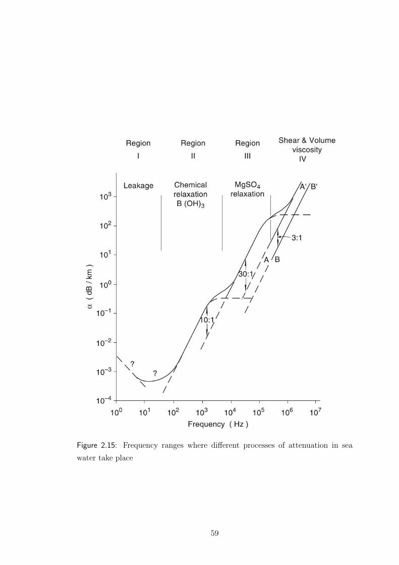
Figure 2.15: Frequency ranges where different processes of attenuation in sea
water take place
59

2.4 Bottom Interaction
When we want to study what happens to a propagating ray when it interacts
with the seafloor it is necessary to deal some preliminary considerations.
First of all, it is required to decide which seabed model to adopt. The ocean
bottom is often modeled as fluids.
This means that the bottom supports only compressional waves. Such an ap-
proximation is appropriate if the seafloor is made of a sufficiently thick layer of
sediments. If this is not true, that is, if sound interacts directly with the base-
ment, the bottom of the ocean has to be modeled as an elastic body, which means
it supports both compressional and shear waves.
In reality the seabed is a viscoelastic body, meaning that it is also lossy.Accurately
modeling bottom interactions is the key to properly predict the propagation of
sound, especially when many interactions with the boundaries take place.
A geoacoustic model is generally chosen as a model of the real seafloor.
On the other hand, the full geoacoustic model is complicated as it depends on
many parameters such as the compressional wave speed, the shear wave speed,
the compressional wave attenuation and so on.
In order to get an overview on what happens when sound interacts with the
bottom, we can analyze the model discussed above, which models bottom as
fluid.
We can consider reflection at an interface separating two homogeneous fluid media
with density ρi and speed of sound ci. We can write the acoustic pressure as
pi = exp(ik1(x cos θ1 + z sin θ1)) (2.1)
pr = R exp(ik1(x cos θ1 − z sin θ1)) (2.2)
pt = T exp(ik2(x cos θ1 + z sin θ2)) (2.3)
By imposing the continuity of pressure, we get
1 +R = T exp(i(k2 cos θ2 − k1 cos θ1)x)
60
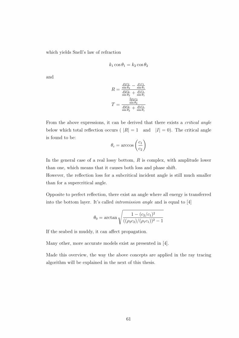
which yields Snell’s law of refraction
k1 cos θ1 = k2 cos θ2
and
R =
ρ2c2sin θ2− ρ1c1
sin θ1ρ2c2sin θ2
+ ρ1c1sin θ1
T =
2ρ2c2sin θ2
ρ2c2sin θ2
+ ρ1c1sin θ1
From the above expressions, it can be derived that there exists a critical angle
below which total reflection occurs ( |R| = 1 and |I| = 0). The critical angle
is found to be:
θc = arccos
(c1c2
)In the general case of a real lossy bottom, R is complex, with amplitude lower
than one, which means that it causes both loss and phase shift.
However, the reflection loss for a subcritical incident angle is still much smaller
than for a supercritical angle.
Opposite to perfect reflection, there exist an angle where all energy is transferred
into the bottom layer. It’s called intromission angle and is equal to [4]
θ0 = arctan
√1− (c2/c1)2
((ρ2c2)/(ρ1c1))2 − 1
If the seabed is muddy, it can affect propagation.
Many other, more accurate models exist as presented in [4].
Made this overview, the way the above concepts are applied in the ray tracing
algorithm will be explained in the next of this thesis.
61


Chapter 3
Implementation Of A Ray Tracer
for Underwater Sound
Propagation Modeling Using
CUDA
3.1 Introductory material
The sound propagation in the ocean, is mathematically described by a set of
equations collectively referred to as the wave equations.
The wave equations form the foundation over which several models have been
developed [4].
Five models are typically used to describe the sound propagation:
• fast field program model
• normal mode model
• ray model
• parabolic equation model
• finite difference model
63

The work presented in the following is focused on a fast algorithm to solve the
wave equations based on the Ray Model approach.
The ray model method was widely used in the middle of the twentieth century
and is still considered a good trade-off between the computational complexity
required to find a solution to the wave equations and the accuracy of the solution
found. While other methods for solving the wave equations have been developed
to date their computational requirements are much greater than those of the ray
model [4]. We will focus on the latter in what follows.
Moreover, its numerical implementation shows many possibilities of improvement
upon which it has been decided to investigate.
3.1.1 A Brief Mathematical Introduction
The study of sound propagation starts from the Helmholtz equation in Cartesian
coordinates.
∇2p+ω2
c2(x)p = −δ(x− x0) (3.1)
where
• p(x) is the complex value of sound pressure
• ω is the angular frequency of the source
• c2(x) is the speed of sound at the coordinates x = (x, y, z)
• δ(· ) is the Dirac delta function
In order to get some equations describing the ray path, we look for a particular
solution of the Helmholtz equation written in the form
p(x) = eiωτ(x)∞∑j=0
Aj(x)
(iω)j
This form of the Helmholtz equation is known in the literature as the ray series.
By differentiating this solution twice and by substituting it into the Helmholtz
64

equation (3.1) we get
eiωτ(x)
[(−ω2|∇τ |2 + iω∇2τ)
∞∑j=0
Aj(iω)j
+ 2iω∇τ∞∑j=0
∇Aj(iω)j
+∞∑j=0
∇2Aj(iω)j
]+
ω2
c2(x)p = −δ(x−x0)
After some algebra, it can be seen that this form of the Helmholtz equation can
be parted into sub-equations as followsO(ω2) : |∇τ |2 = 1
c2(x)
O(ω) : 2∇τ · ∇ A0 + (∇2τ)A0 = 0
O(ω1−j), j = 1, 2, · · · : 2∇τ · ∇ Aj + (∇2τ)Aj = −∇2Aj−1
The O(ω2) equation is known under the name of Eikonal equation. The other
equations are generally referred to as transport equations.
The power of such form is than not solving all sub-equations is necessary, but
just solving both the Eikonal equation and the highest order transport equation
produce the results we are seeking.
As we will see later in more detail, the solution to the Eikonal equation is re-
quired in order to get the trajectory and phase of the ray, whereas the transport
equation gives information on the ray amplitude, which is required to find the
sound pressure.
Eikonal Equation
What it is expected from the Eikonal equation solution is the ray path, hence we
can define the ray trajectory as
dx
ds= c∇τ
where s represents the arc-length of the ray.
By differentiating this equation with respect to s we get (considering only the
x-component)
d
ds
(1
c
dx
ds
)=
d
ds
(dτ
dx
)=c
2
d
dx
[(dτ
dx
)2
+
(dτ
dy
)2]
=c
2
d
dx|∇τ |2
65

then by using the Eikonal equation and by repeating the procedure for other
coordinates, we obtain the equations for the ray path:
d
ds
(1
c
dx
ds
)+
1
c2dc
dx= 0
d
ds
(1
c
dy
ds
)+
1
c2dc
dy= 0
d
ds
(1
c
dz
ds
)+
1
c2dc
dz= 0
Rewriting them in cylindrical coordinates (r, z) we get
dr
ds= c· ξ(s) dξ
ds= − 1
c2dc
drdz
ds= c· ζ(s)
dζ
ds= − 1
c2dc
dz
where the auxiliary variables ξ and ζ have been introduced in order to write the
ray equations in the first order form.
Solving these differential equations, it is possible to obtain the trajectory of the
ray as shown in figure 3.1.
Figure 3.1: trajectory of a ray computed solving the ray equations
66

Many times it is useful to have equations with the range as the independent
variable instead of s.
To get it we can proceed as follows. By dividing the ray equations by dzds
we
obtain
dz
dr=ζ
ξ(3.2)
dξ
dz= − 1
c3ζ
dc
dr(3.3)
dζ
dz= − 1
c3ζ
dc
dz(3.4)
Then increasing the differential order of (3.2) and substituting on it the equations
(3.3) and (3.4), it becomes
d2r
dz2=
dcdz− ξ
ζdcdr
c3ζ2(3.5)
Moreover, rearranging the ray equation is possible to write it as
ζ2 =1
c2
(dr
ds
)2
=1
c21
1 + ( drdz
)2(3.6)
Now using (3.5) and (3.6), we obtain the following differential ray equation for
the ray range r as a function of z.
d2r
dz2=
[1 +
(dr
dz
)2][
1
c
(dr
dz
)dc
dz− 1
c
dc
dr
](3.7)
Following the same steps, it is possible to obtain the ray depth z as a function of
r.
The ray equations written in these forms point out the dependency of the trajec-
tory from the variation of c, both in range and in depth.
As we have seen in the previous chapter, the value of the speed of sound is very
sensitive with respect to changes in depth.
On the contrary, in general, the variations of the sound speed in a seawater envi-
ronment for a fixed depth around a sound source are negligible.
Therefore, the suppression of range dependency in c is a common procedure that
allows to greatly simplify ray equations.
In fact, (3.7) becomes
d2r
dz2=
1
c
dr
dz
dc
dz
(1 +
(dr
dz
)2)
67

After working out a few mathematic calculations, it produces a more handy
solution
r(z) = r(z0) +
∫ z
z0
ac√1− a2c2
dz′ (3.8)
3.1.2 Stratified media
In general, the more detailed the knowledge of c is, the more accurate the calcu-
lated path will be.
The information we get about the values of c is derived from periodical measures
of water column features, which provide tabulated value of c.
Moreover, to perform the computation of the ray trajectory, we need a continuous
function representing c. Therefore, a classical interpolation problem arises.
Interpolation of data is a problem deeply studied in literature and tens of algo-
rithms exist.
In order to accomplish our aim, the use of the linear interpolation is the right
choice, guaranteeing an acceptable correctness and a simple management. We
will refer to a medium where the speed of sound is linearly interpolated using the
term “c-linear” medium.
With this choice, the water column can be viewed as a stack of c-linear layers,
i.e., a stratified medium.
The boundaries of each layer are represented by two successive points of the
tabulated sound speed profile.
Within each layer, the speed of sound can be expressed simply as
c(z) = c0 + gz
where c0 is the y-intercept of the line passing through two successive sound speed
profile points and g is the line slope.
Having defined c(z) in such a way, equation (3.8) can be easily integrated yielding
r(z) = r(z1) +
√1− a2c2ag
∣∣∣∣c(z)c(z1)
This equation can be rearranged in the typical form of the circumferences
(r − (r(z1)− b))2 +
(z +
c0g
)2
= R2
68

where
R =1
ag(3.9)
b =
√1− a2(c0 + gz1)2
ag(3.10)
are respectively the radius and the range coordinate of the circle center.
The circumference center’s depth is placed where the speed of sound vanishes,
that is, at z = − c0g
.
Therefore, in a c-linear media the ray follows a circular trajectory as showed in
figure 3.2
III
III IV
range
dept
h
R
Figure 3.2: Trajectory of a ray in a c-linear medium: the trajectory cases I, II,
III and IV occur depending both on the ray departure angle and on the slope of
c line within the layer
3.1.3 Path in the whole stratified medium
As previously discussed, to assume that c is range-independent throughout the
medium is very handy; along with linear interpolation, this provides a very simple
69

function describing the variation of the speed of sound between two tabulated
depths.
Using this approach, the environment can be represented as a layered medium as
figure 3.3 shows. Figure 3.3 also shows that the water column can be modeled as
stack of c-linear layers.
In order to compute the entire path of the ray in the medium, for each c-linear
layer we can compute the circular trajectory of the ray, and joint the circle arcs
contained between the boundaries of the layers.
Figures 3.4a, 3.4b, 3.4c, 3.4d and 3.5 show some possible examples.
z
rc
Figure 3.3: A piecewise-linear sound speed profile gives rise to a layered medium
70

range
dept
h
range
dept
h
range
dept
h
range
dept
h
Figure 3.4: Examples of ray trajectory within a layer, corresponding to the cases
I, II, III, and IV in Fig. 3.2
dept
h
range
Figure 3.5: All trajectories computed inside every layer are linked together yield-
ing the complete ray trajectory
71

3.2 CUDA Algorithm
As explained in Section 1.2, when a programming parallel software it is necessary
to identify which parts of the algorithm can be well parallelized, and which cannot.
Generally, an algorithm solving real problems is made by a mix of the two cases
above and therefore its common execution path could appears like the following:
sync
sync sync
sync & share point
Figure 3.6: A typical program run path
Since we desire to develop an algorithm well suited for the CUDA program-
ming model, we must identify where parallelization works and where it has to be
stopped, turning back to a serial execution path. Going back to the circular ray
trajectory introduced in Section 3.1 it can be seen that once the circle parameters
are known, the computation of the trajectory inside a layer needs nothing more.
Hence it can be parallelized.
Therefore the tracing algorithm has been designed with two level of paralleliza-
tion:
• Parallelization across the rays. Every CUDA threads block computes
the trajectory of six rays.
• Parallelization of the ray. 32 threads work at the same time on every
ray.
This means that there are 192 active threads on every CUDA block. This choice
has been made in order to not overload the GPU (see Section 1.6.3).
The ray tracing theory assumes that the rays are independent each other, hence
the parallelization between rays can be full.
72
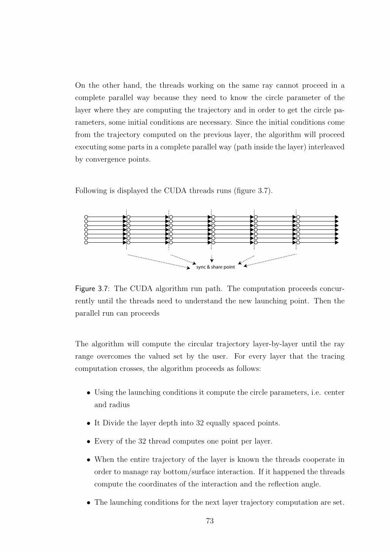
On the other hand, the threads working on the same ray cannot proceed in a
complete parallel way because they need to know the circle parameter of the
layer where they are computing the trajectory and in order to get the circle pa-
rameters, some initial conditions are necessary. Since the initial conditions come
from the trajectory computed on the previous layer, the algorithm will proceed
executing some parts in a complete parallel way (path inside the layer) interleaved
by convergence points.
Following is displayed the CUDA threads runs (figure 3.7).
sync
sync sync
sync & share point
Figure 3.7: The CUDA algorithm run path. The computation proceeds concur-
rently until the threads need to understand the new launching point. Then the
parallel run can proceeds
The algorithm will compute the circular trajectory layer-by-layer until the ray
range overcomes the valued set by the user. For every layer that the tracing
computation crosses, the algorithm proceeds as follows:
• Using the launching conditions it compute the circle parameters, i.e. center
and radius
• It Divide the layer depth into 32 equally spaced points.
• Every of the 32 thread computes one point per layer.
• When the entire trajectory of the layer is known the threads cooperate in
order to manage ray bottom/surface interaction. If it happened the threads
compute the coordinates of the interaction and the reflection angle.
• The launching conditions for the next layer trajectory computation are set.
73

In the next, the above steps are described in more detail.
Launching Conditions And Circle parameters
At this point it should be clear that for every layer it is necessary to know the circle
parameters that make it possible to compute the ray trajectory using Equation
(3.8).
To get the parameters we need, it is required that some initial conditions have
been set by the previous-layer iteration. It is necessary to know the coordinate
of the last trajectory point computed from which the computation restarts and
the ray angle at this point.
If the iteration is the first, the initial conditions are the coordinates of the sound
source and the ray angle at the source. The source ray angle is derive as
StartAngle+StartAngle− EndAgnle
Nrays∗RayID (3.11)
where
• the StartAngle(EndAngle) is the maximum(minimum) angle value span on
which the rays are computed
• the Nrays is the number of the ray computed by the simulation
• the RayID is the numerical identifier of the ray.
By the knowledge of these starting parameters the algorithm can continue. First,
is necessary to know on which layer we are in. This is accomplished using the
function
1 i = wws2(&livello[0], zIn, orders[y ].Aing, maxIndexLayer);
that using the ray angle and the ray deepness, furnishes the layer’s ID number,
i.e. a numeric identifier assigned to every layer, we are looking for.
The ray angle is necessary only if the starting point lands on the interface between
two layers, in order to disambiguate on which layer the algorithm will proceed.
74

Finally, when the ID of the layer involved in the computation of the trajectory
piece is known, it is possible to compute the circle parameters.
This is what the next part does, computing the parameters requested.
1 cIn = ssp v2(layer[ i ], zIn) ;
2 a = cosf(orders[y ].Aing)/cIn;
3 z0 = −cIn/layer[i ]. g;
4 R = abs(1/(a ∗ layer[i ]. g)) ;
5 zMax = zIn + z0 + R;
6 zMin = zIn + z0 − R;
Layer Partitioning and Trajectory Points computation
Until we do not leave the layer from where this piece of computation has started,
all trajectory points are simply derived by applying the equation 3.8 with the
circle parameters just calculated.
To obtain the minimum waste of computation time, the layer depth interval is
divided into a set of equally spaced points equal to the threads number involve
in the ray, i.e. 32.
In this way, every thread computes only one trajectory point per layer. The
following listing does what above, setting a depth coordinate point on which the
thread will compute the related range. Using that into (3.8), the CUDA thread
computes the correspondent range point.
1 if (orders[y ].Aing > 0 )
2 {3 dz = (layer[ i ]. zIn + layer[ i ]. Dz − zIn) / Nthr;
4 point.y = zIn + (x+1) ∗ dz;
5 }6 else if ( orders[y ].Aing < 0 )
7 {8 dz = (zIn − layer[ i ]. zIn) / Nthr;
9 point.y = zIn − (x+1) ∗ dz;
10 }11 else if ( orders[y ].Aing == 0 && abs(zIn− zMax) < abs(zIn− zMin) )
75

12 {13 zIn = zMax;
14 dz = (zIn − layer[ i ]. zIn) / Nthr;
15 point.y = zIn − (x+1) ∗ dz;
16 }17 else if ( orders[y ].Aing == 0 && abs(zIn− zMax) > abs(zIn− zMin) )
18 {19 zIn = zMin;
20 dz = (layer[ i ]. zIn + layer[ i ]. Dz − zIn) / Nthr;
21 point.y = zIn + (x+1) ∗ dz;
22 }23 if ( point.y >= zMax )
24 {25 point.y = zMax;
26 }27 if ( point.y <= zMin )
28 {29 point.y = zMin;
30 }31 if (point.y <= layer[i ]. zIn)
32 {33 point.y = layer[ i ]. zIn;
34 }35 if ( point.y >= layer[i ]. zIn + layer[ i ]. Dz )
36 {37 point.y = layer[ i ]. zIn + layer[ i ]. Dz;
38 }
Moreover, the previous code guarantee to avoid the computation of points outside
the depth interval [zMin, zMax] necessary to be inside the domain of the function
(3.8).
Another approach has also been developed, allowing users to fix the depth vari-
ation. However, if it is not strictly necessary, this second approach should be
deprecated since it introduced some waste of resources, and degrades the perfor-
76

mance of the algorithm.
Boundaries Interaction
We now know of the complete trajectory within the layer where we are computing
the trajectory, so that, we must check if the ray has interacted with the seafloor
(or the surface).
To maintain a small complexity, both the seabed and the surface are treated as
piecewise linear surfaces.
Figure 3.8 shows how we proceed to find the interaction point.
Using some preliminary considerations, it is possible to discard pieces of trajec-
tory that surely can not interact.
interaction point
dept
h
Figure 3.8: pieces of trajectory checked in green, discarded pieces in red
For example checking only the trajectory pieces respecting the following condition
generally saves computation time.
1 if ( bottom[i−1].x <= max(me1.x,me0.x) && bottom[i].x >= min(me0.x,me1.
77

x) && max(bottom[i].y,bottom[i−1].y) >= min(me0.y,me1.y) && min(
bottom[i].y,bottom[i−1].y) <= max(me0.y,me1.y) )
It is useful to point out that the strength of the “filtering” increases if the bound-
ary’s details increases, producing a better performance.
Interaction coordinate
After signaling out the points that may certain can interact with the bottom, it
is necessary to find the coordinates of the interaction.
For every trajectory segment chosen in the previous step (green pieces of the im-
age 3.8), we derive the equation of the line joining the two points of the trajectory.
Then using the line equation of the bottom segment, if the lines are not parallel,
crossing points between them always exists.
Moreover, checking the position of the computed crossing points, it is easy to
understand which of them is the actual interaction point. Figure 3.9 shows an
example.
78

interaction point
dept
h
Figure 3.9: Only one interaction point exists. It is located inside the green section
of the trajectory
The following part of the code shows how the above is done.
1 float m =( me1.y − me0.y ) / ( me1.x − me0.x);
2 float rm = m / bottom[i−1].z;
3 if (rm == 1) return false;
4 y = (q − rm ∗ bottom[i−1].w) / (1 − rm);
5 if ( y <= max(me0.y, me1.y) && y >= min(me0.y, me1.y) && y != zIn )
6 {......}
Since not leaving threads idle is a fundamental guide line of the CUDA program-
ming, each thread checks one segment of the trajectory.
Reflection angle
Once we get the interaction point coordinate (if an interaction happened), the
next necessary step is to understand which is the new launching angle.
As [4] explains, the problem can be solved on noting that the tangent of the
79

reflected ray can be expressed as
tref = tinc − 2(tinc · nbot)nbot (3.12)
where
• tinc is the tangent of the interacting ray
• nbot is the normal of the bottom
• · is the inner product
Therefore, using these two easily computable parameters, we can compute the
rebound angle we are looking for.
Setting the starting conditions for the next iteration
When the above steps have been executed, the threads are able to understand
which is the last valid trajectory point, and set it as starting point for the next
iteration.
If no interaction has taken place, it is the point computed by the last thread,
i.e. the 32-th threads. Opposite, if the interaction happened, the next iteration
starting coordinates are those of the interaction point and the launching angle is
the reflection angle on the bottom/surface.
3.3 Performance
As widely discussed in the first chapter, in order to get good performance when
running CUDA applications it is absolutely necessary to carefully handle the
memory.
To this end, we have adopted the 2-D matrix structure displayed in figure 3.10.
Using this structure helps to use the graphic card memory transactions at their
full capabilities.
The shape of the block of threads has been set to contain 192 threads, placed in
an ideal 6 x 32 matrix.
80

points
rays
Figure 3.10: 2-D matrix used to save trajectory data
There are 32 threads working on every ray, and 6 rays per block, hence every
matrix row is related to one ray.
This design makes every threads block “moving” toward the right direction, tak-
ing advantage from coalesced memory transactions. Figure 3.11 shows it in detail.
Summarizing, setting the number of threads to 192 guarantees the maximum
occupancy of the stream processors, whereas the threads matrix shape ensures
the best data bandwidth.
81

Block of
Threads
Block of
Threads
points
rays
Block of
Threads
Figure 3.11: Block of threads data managements
A speed test has been performed, comparing the classical serial implementation
of the tracer and the GPU-powered implementation on an shallow water scenario
(the most computationally challenging because of the high numbers of seabed/-
surface interactions).
Bellhop
Bellhop is a well known an widely used underwater simulation program imple-
menting the classical single thread execution.
bellhop is able to compute both the rays trajectory and the pressure field. Since
the ray tracing is the skeleton for the pressure computation, this computation is
always performed by the bellhop. If the pressure is not requested the software
ends its run, whereas if the user needs the pressure field, Bellhop derives the
pressure values using the rays trajectory already computed.
The ray tracing method is performed by a function named Trace. On it, solv-
82

ing the ray equations and the dynamic ray equation [7], Bellhop computes the
trajectory points but also other parameters requested for the next pressure com-
putation.
In order to equally compare the two implementations, the Bellhop has been mod-
ified. All the actions performed into the Trace function not necessary to the
trajectories computing have been removed.
Execution times have been obtained by profiling the software and considering the
time to execute the Trace function.
The CUDA accelerated ray tracer
The CUDA implementation of the ray tracer has been timed by using the Nvidia
CUDA profile included into the CUDA SDK. On the CUDA tracer time counting
is included the time necessary to move data from the Host RAM to the Device
RAM and vice versa.
The Tester Systems
The Bellhop test has been executed on the next two systems:
CPU Intel Core 2 Duo E8400 Intel Xeon X5650
@ 3.0 GHz, 6 MB cache @ 2.66 GHz, 12 MB cache
RAM 4 GB DDR2 16 GB DDR3
whereas on the next two has been performed the CUDA runs
CPU Intel i7-2670QM Intel i7-2600
@ 2.2 GHz, 6 MB cache @ 3.4 GHz, 8 MB cache
RAM 8 GB DDR3 16 GB DDR3
GPU Nvidia GT 540M, 2 GB RAM Nvidia GTX 580, 3 GB RAM
83

The results
The times has been collected varying the number of simulated rays. The results
follow.
RaysBellhop time [ms] CUDA time [ms] CUDA Speedup
E8400 X5650 GT 540M GTX 580 X5650/GT 540M X5650/GTX 580
2000 440 440 35.3 9.6 12.5x 45.8x
5000 1191 1142 92.4 24.1 12.4x 47.4x
10000 2405 2154 176.5 47.6 12.2x 45.3x
20000 5313 4133 392.8 95.6 10.5x 43.2x
40000 10178 8150 787.0 258.0 10.4x 31.6x
60000 16270 12212 1179.0 284.8 10.4x 42.9x
2000 5000 10000 20000 40000 600000
2000
4000
6000
8000
10000
12000
14000
16000
18000
Number of rays computed
Tim
e of
exe
cutio
n[m
s]
Computation Time
E8400X5650GT 540MGTX 580
Figure 3.12: The Simulation time vs. the number of simulated rays
The results show the power of the CUDA implementation.
On average, comparing the CUDA results with those reached using the Xeon,
the running time on a very low-cost graphic such as the GT 540M card is 11.3
times faster than the Xeon based computer, whereas using the GTX device the
computation is performed 42.8 times faster.
84

3.4 Pressure computation
Once the rays path has been obtained, the next major goal is the computation of
the sound pressure produced by the rays. The theory says that, in order to get
the pressure, it is first necessary for every ray to solve a pair of coupled differential
equations known under the name of Dynamic ray tracing equations (see [4]):
dq
ds= c(s)p(s) (3.13)
dp
ds= − cnn
c(s)2q(s) (3.14)
where s is the arc-length of the ray, c is the speed of sound and p and q are
a couple of complex-value variables that allow to handy compute the pressure
variations imposed by the ray passing.
cnn is the curvature of the sound speed in a direction normal to the ray path.
Using the auxiliary variables ξ and ζ introduced on Section 3.1.1, cnn can be
expressed as:
cnn = c
(d2c
dr2ζ2 − 2
d2c
drdzζξ +
d2c
dz2ξ2)
It is now possible to compute the influence of every ray onto a “receivers’s” grid.
The receivers grid is an ideal grid of receivers located at the points where the
sound pressure is required (see an example on figure 3.13). It could be a regular
grid (i.e, a grid with equally spaced points) or not.
Following the suggestion of [4], it can be seen that for every trajectory segment
there could be points far enough from the ray center to not be influenced by
the passing ray. In order to optimize the performance, it is useful to direct the
computation effort on the points of the grid where the sound pressure is in fact
influenced by the ray.
That strategy require that for every ray segment we find a ray influence zone.
Using the values of the q variable is possible to set the vertical boundaries of this
zone of influence, whereas the horizontal zone extremes are equals to the range
coordinates of the ray segment ends.
On the receivers located inside the zone will be computed the ray influence,
whereas on the receivers outside, the computation is avoided, saving the corre-
spondent computation time.
85

Figure 3.13: receivers involved in the computation for a single ray segment
We tried to implements the pressure computation applying the above idea: namely,
every thread computes the influence of a ray segment on the receivers.
It has to be pointed out that every receiver corresponds to a memory location
on the device memory, and unfortunately, this kind of approach imposes a spare
memory access pattern that is badly managed by the CUDA architecture (see
Section 1.6.5).
An alternative approach has also been tested. The “focus” is moved to the
receivers. That means that a number of threads blocks equal to the number of
the receivers has been created. Every block takes care of only one receiver and
the threads of the block compute the influence of all the simulated rays on that
particular receiver assigned to the block.
Opposite to what happens on the first implementation, the receiver grid memory
access issue does not take place any more, but now, the problem is represented
by the ray trajectory memory handling.
Moreover, numerical integrators proceed step by step, and are an example of
algorithm that it is difficult to parallelize.
With all this said, it possible to understand why the simulations performed on
86

the pressure computing exhibit a running time comparable to the classical CPU
implementation, or sometimes worse (because of memory transfers).
This is the reason why we have preferred to maintain these functions performed
by a classical CPU run.
87


Conclusions
The primary goal of this thesis is to provide a fast tool able to simulate an
underwater sound channel. The necessity arose because the existing software is
usually too slow to satisfy the present speed requirements.
To solve this issue we decided to develop a parallel version of ray tracing software
Bellhop.
This has been identified as the best choice since the classical underwater simula-
tion issue is complex but also repeating, i.e., computing the solution in a parallel
way gives benefits.
Between various possibilities, it has been decided to approach the issue using
the brand new NVIDIA graphic cards enabled to provide an all-in-one parallel
computation system at a good price.
The GPU-powered ray tracer has been developed by using two levels of paral-
lelization, both between the rays and inside every ray.
If the parallelization between the rays derives from the fundamental characteristic
of the ray tracing methods, the parallelization inside the rays could has been done
because of the using of the common assumption of a stratified medium, allows to
model the ray paths as piecewise circular trajectories, whose computation can be
subdivided among the treads.
By designing the software following this guideline, we obtained a software fully
benefiting by the execution on a CUDA device.
The algorithm exhibits a considerable speedup if compared with the “classical”
serially running algorithm.
89

Referring to a Xeon provided systems, the CUDA tracer exhibit a performance
improvement of 11.3 times if compared with the entry-level GT 540M graphic
card and of 42.8 times if compare with a more powerful GTX 580.
The extremely interesting feature of this approach is that the speedup is of course
related with the power of the GPU used, but it occurs also using an entry-level
low-price graphic cards as the GT 540M.
It has to be underlined that not the whole Bellhop software has been redesigned to
run on GPUs. This choice because of the strictly serial execution nature of some
algorithm parts, e.g. the numerical integration, and because of some constraints
imposed by the CUDA architecture.
Hence, the optimal final solution that could be built in future will be an hybrid
program where each processing unit is employed to do the kind of work it does
best: pressure computation performed by the Bellhop, and trajectory tracing
performed on by the GPU.
In conclusion, performing this work, the intent was to provide a first step toward
a real decreasing of the ratio between the “systems price” and the computation
time on the underwater sound propagation simulation, hoping that it could be
useful in both the actual and the next generation underwater networks design
and management.
90

Bibliography
[1] Ainslie M. A. and McColm J. G. A simplified formula for viscous and chem-
ical absorption in sea water. Journal of the Acoustical Society of America,
103(3):1671–1672, 1998.
[2] NVIDIA Corporation. Cuda c best practices guide, 2011.
[3] NVIDIA Corporation. Cuda c programming guide, 2011.
[4] F.B. Jensen, W.A. Kuperman, M.B. Porter, and H. Schmidt. Computational
Ocean Acoustics. Springer-Verlag, New York, 2 edition, 1984. 2nd printing
2000.
[5] David B. Kirk and Wen mei W. Hwu. Programming massively parallel pro-
cessor. Morgan Kaufmann, 2010.
[6] H. Medwind and C.S. Clay. Fundamentals of acoustical oceanography. Aca-
demic, San Diego, 1997.
[7] M.B. Porter and Y-C Liu. Finite elements ray tracing. Proceedings of the
International Conference on Theoretical and Computational Acoustics, pages
947–956, 1994.
[8] Jason Sanders and Edward Kandrot. CUDA by Example: An Introduction to
General-Purpose GPU Programming. Addison-Wesley Professional, 2010.
[9] R.J. Urick. Sound propagation in the sea. Defense Advanced Research Project
Agency, Washington DC, 1979.
91