Parallel and Distributed Simulation of Discrete Event SystemsAlois Ferscha� Satish K. TripathiInstitut f�ur Angewandte Informatik Computer Science DepartmentUniversit�at Wien University of MarylandLenaugasse 2/8, A-1080 Vienna, AUSTRIA College Park, MD 20742, U.S.A.Email: ferscha@ani.univie.ac.at Email: tripathi@cs.umd.eduAbstractThe achievements attained in accelerating the simulation of the dynamics of complex discreteevent systems using parallel or distributed multiprocessing environments are comprehensivelypresented. While parallel discrete event simulation (DES) governs the evolution of the systemover simulated time in an iterative SIMD way, distributed DES tries to spatially decompose theevent structure underlying the system, and executes event occurrences in spatial subregions bylogical processes (LPs) usually assigned to di�erent (physical) processing elements. Synchroniza-tion protocols are necessary in this approach to avoid timing inconsistencies and to guaranteethe preservation of event causalities across LPs.Included in the survey are discussions on the sources and levels of parallelism, synchronousvs. asynchronous simulation and principles of LP simulation. In the context of conservative LPsimulation (Chandy/Misra/Bryant) deadlock avoidance and deadlock detection/recovery strate-gies, Conservative Time Windows and the Carrier Nullmessage protocol are presented. Relatedto optimistic LP simulation (Time Warp), Optimistic Time Windows, memory management,GVT computation, probabilistic optimism control and adaptive schemes are investigated.CR Categories and Subject Descriptors: C.1.0 [Processor Architectures:] General; C.2 [Computer Communi-cation Networks:] Distributed Systems | Distributed Applications; C.4 [Computer Systems Organization:]Performance of Systems | Modeling techniques; D.4.1 [Operating Systems:] Process Management | Concur-rency, Deadlocks, Synchronization; I.6.0 [Simulation and Modeling:] General; I.6.8 [Simulation and Modeling:]Types of Simulation { Distributed, ParallelGeneral Terms: Algorithms, PerformanceAdditional Key Words and Phrases: Parallel Simulation, Distributed Simulation, Conservative Simulation, OptimisticSimulation, Synchronization Protocols, Memory Management�This work was conducted while Alois Ferscha was visiting the University of Maryland, Computer Science De-partment, supported by a grant from the Academic Senate of the University of Vienna.1

Contents1 Introduction 31.1 Continuous vs. Discrete Event Simulation : : : : : : : : : : : : : : : : : : : : : : : : 31.2 Time Driven vs. Event Driven Simulation : : : : : : : : : : : : : : : : : : : : : : : : 41.3 Accelerating Simulations : : : : : : : : : : : : : : : : : : : : : : : : : : : : : : : : : : 51.3.1 Levels of Parallelism/Distribution : : : : : : : : : : : : : : : : : : : : : : : : 61.4 Parallel vs. Distributed Simulation : : : : : : : : : : : : : : : : : : : : : : : : : : : : 71.5 Logical Process Simulation : : : : : : : : : : : : : : : : : : : : : : : : : : : : : : : : 81.5.1 Synchronous LP Simulation : : : : : : : : : : : : : : : : : : : : : : : : : : : : 91.5.2 Asynchronous LP Simulation : : : : : : : : : : : : : : : : : : : : : : : : : : : 102 \Classical" LP Simulation Protocols 112.1 Conservative Logical Processes : : : : : : : : : : : : : : : : : : : : : : : : : : : : : : 112.1.1 Deadlock Avoidance : : : : : : : : : : : : : : : : : : : : : : : : : : : : : : : : 122.1.2 Example: Conservative LP Simulation of a PN with Model Parallelism : : : : 142.1.3 Deadlock Detection/Recovery : : : : : : : : : : : : : : : : : : : : : : : : : : : 172.1.4 Conservative Time Windows : : : : : : : : : : : : : : : : : : : : : : : : : : : 182.1.5 The Carrier Null Message Protocol : : : : : : : : : : : : : : : : : : : : : : : : 192.2 Optimistic Logical Processes : : : : : : : : : : : : : : : : : : : : : : : : : : : : : : : : 202.2.1 Time Warp : : : : : : : : : : : : : : : : : : : : : : : : : : : : : : : : : : : : : 202.2.2 Rollback and Annihilation Mechanisms : : : : : : : : : : : : : : : : : : : : : 232.2.3 Optimistic Time Windows : : : : : : : : : : : : : : : : : : : : : : : : : : : : : 262.2.4 The Limited Memory Dilemma : : : : : : : : : : : : : : : : : : : : : : : : : : 262.2.5 Incremental and Interleaved State Saving : : : : : : : : : : : : : : : : : : : : 272.2.6 Fossil Collection : : : : : : : : : : : : : : : : : : : : : : : : : : : : : : : : : : 282.2.7 Freeing Memory by Returning Messages : : : : : : : : : : : : : : : : : : : : : 292.2.8 Algorithms for GVT Computation : : : : : : : : : : : : : : : : : : : : : : : : 332.2.9 Limiting the Optimism to Time Buckets : : : : : : : : : : : : : : : : : : : : : 372.2.10 Probabilistic Optimism : : : : : : : : : : : : : : : : : : : : : : : : : : : : : : 393 Conservative vs. Optimistic Protocols? 434 Sources of Literature and Further Reading 462

1 IntroductionModeling and analysis of the time behavior of dynamic systems is of wide interest in various�elds of science and engineering. Common to `realistic' models of time dynamic systems is theircomplexity, very often prohibiting numerical or analytical evaluation. Consequently, for those cases,simulation remains the only tractable evaluation methodology. Conducting simulation experimentsis, however, time consuming for several reasons. First, the design of su�ciently detailed modelsrequires in depth modeling skills and usually extensive model development e�orts. The availabilityof sophisticated modeling tools today signi�cantly reduces development time by standardized modellibraries and user friendly interfaces. Second, once a simulation model is speci�ed, the simulationrun can take exceedingly long to execute. This is due either to the objective of the simulation, orthe nature of the simulated model. For statistical reasons it might for example be necessary toperform a whole series of simulation runs to establish the required con�dence in the performanceparameters obtained by the simulation, or in other words make con�dence intervals su�cientlysmall. Another natural consequence why simulation should be as fast as possible comes from theobjective of exploring large parameter spaces, or to iteratively improve a parameter estimate in aloop of simulation runs. The simulation model as such might require tremendous computationalresources, making the use of contemporary 100 MFLOPs computers hopeless.Possibilities to resolve these shortcomings can be found in several methods, one of which is theuse of statistical knowledge to prune the number of required simulation runs. Statistical methodslike variance reduction can be used to avoid the generation of \unnecessary" system evolutions, inthe sense that statistical signi�cance can be preserved with a smaller number of evolutions given thevariance of a single random estimate can be reduced. Importance sampling methods can be e�ectivein reducing computational e�orts as well. Naturally, however, faster simulations can be obtainedby using more computational resources, particularly multiple processors operating in parallel. Itseems obvious at least for simulation models re ecting real life systems constituted by componentsoperating in parallel, that this inherent model parallelism could be exploited to make the use of aparallel computer potentially e�ective. Moreover, for the execution of independent replications ofthe same simulation model with di�erent parametrizations the parallelization appears to be trivial.In this work we shall systematically describe ways of accelerating simulations using multiprocessorsystems with focus on the synchronization of logical simulation processes executing in parallel ondi�erent processing nodes in a parallel or distributed environment.1.1 Continuous vs. Discrete Event SimulationBasically every simulation model is a speci�cation of a physical system (or at least some of itscomponents) in terms of a set of states and events. Performing a simulation thus means mimickingthe occurrence of events as they evolve in time and recognizing their e�ects as represented bystates. Future event occurrences induced by states have to be planned (scheduled). In a continuoussimulation, state changes occur continuously in time, while in a discrete simulation the occurrenceof an event is instantaneous and �xed to a selected point in time. Because of the convertability ofcontinuous simulation models into discrete models by just considering the start instant as well asthe end instant of the event occurrence, we sill subsequently only consider discrete simulation.3

VT

EVL

S

e i e j e k

s 1 s 2 s 3 s 4 s NFigure 1: Simulation Engine for Discrete Event Simulation1.2 Time Driven vs. Event Driven SimulationTwo kinds of discrete simulation have emerged that can be distinguished with respect to the waysimulation time is progressed. In time driven discrete simulation simulated time is advanced in timesteps (or ticks) of constant size �, or in other words the, observation of the simulated dynamicsystem is discretized by unitary time intervals. The choice of � interchanges simulation accuracyand elapsed simulation time: ticks short enough to guarantee the required precision generallyimply longer simulation time. Intuitively, for event structures irregularly dispersed over time, thetime-driven concept generates ine�cient simulation algorithms.Event driven discrete simulation discretizes the observation of the simulated system at eventoccurrence instants. We shall refer to this kind of simulation as discrete event simulation (DES)subsequentially. A DES, when executed sequentially repeatedly processes the occurrence of eventsin simulated time (often called \virtual time", VT) by maintaining a time ordered event list (EVL)holding timestamped events scheduled to occur in the future, a (global) clock indicating the currenttime and state variables S = (s1; s2; : : :sn) de�ning the current state of the system (see Figure 1).A simulation engine (SE) drives the simulation by continuously taking the �rst event out of theevent list (i.e. the one with the lowest timestamp), simulating the e�ect of the event by changingthe state variables and/or scheduling new events in EVL { possibly also removing obsolete events.This is performed until some pre-de�ned endtime is reached, or there are no further events to occur.As an example, assume a physical system of two machines participating in a manufacturingprocess. In a preprocessing step, one machine produces two subparts A1 and A2 of a productA, both of which can be assembled concurrently. Part A1 requires a single, whereas A2 takes anonpredictable amount of assembly steps. Once one A1 and one A2 are assembled (irrespective ofthe machine that assembled it) one piece of a A is produced.The system is modelled in terms of a Petri net (PN): transition t1 models the preprocessingstep and the forking of independent postprocessing steps, t2 and t3. Machines in the preprocessingphase are represented by tokens in p1, �nished parts A1 by tokens in p5 and �nished or \still inassembly" parts A2 by tokens in p4. Once there is at least one token in p5 and at least one token inp4, the assembly process stops or repeats with equal probability (con ict among t4 and t5). Oncethe assembly process terminates yielding one A, one machine is released (t5). The time behaviorof the physical system is modelled by associating timing information to transitions (�(t1) = 3,�(t2) = �(t3) = 2 and �(t4) = �(t5) = 0). This means that a transition ti that became enabled bythe arrival of tokens in the input places at time t and remained enabled (by the presence of tokensin the input places) during [t; t + �(ti)). It �res at time t + �(ti) by removing tokens from input4

places and depositing tokens in ti's output places. The initial state of the system is represented bythe marking of the PN where place p1 has 2 tokens (for 2 machines), and no tokens are availablein any other place. Both the time driven and the event driven DES of the PN are illustrated inFigure 2.The time driven DES increments VT (denoted by a watch symbol in the table) by one timeunit each step, and collects the state vector S as observed at that time. Due to time resolution andnon time consuming state changes of the system, not all the relevant information could be collectedwith this simulation strategy.The event driven DES employs a simulation engine as in Figure 1 and exploits a natural corre-spondence among event occurences in the physical system and transition �rings in the PN modelby relating them: whenever an event occurs in the real (physical) system, a transition is �red in themodel. The event list hence carries transitions and the time instant at which they will �re, giventhat the �ring is not preempted by the �ring of another transition in the meantime. The state ofthe system is represented by the current PN marking (S), which is changed by the processing ofan event, i.e. the �ring of a transition: the transition with the smallest timestamp is withdrawnfrom the event list, and S is changed according to the corresponding token moves. The new state,however, can enable new transitions (in some cases maybe even disable enabled transitions), suchthat EVL has to be corrected accordingly: new enabled transitions are scheduled with their �ringtime to occur in the future by inserting them into EVL (while disabled transitions are removed).Finally the VT is set to the timestamp (ts) of the transition just �red.Related now to the example in Figure 2 we have: Before the �rst step of the simulation starts,VT is set to 0 and transition t1 is scheduled twice for �ring at time 0 + �(t1) = 3 according to theinitial state S = (2; 0; 0; 0; 0). There are two identical event entries with identical timestamps inthe EVL, announcing two event occurrences at that time. In the �rst simulation step, one of theseevents (since both have identical, lowest timestamps) is taken out of EVL arbitrarily, and the stateis changed to S = (1; 1; 1; 0; 0) since �ring t1 removes one token from p1 and generates one token forboth p2 and p3. Finally VT is adjusted. The new marking now enables transitions t2 and t3, bothwith �ring time 2. Hence, new event tuples ht2@VT + �(t2)i and ht3@VT + �(t3)i are generatedand scheduled, i.e. inserted in EVL in increasing order of timestamp. In step 2, again, the eventwith smallest timestamp is taken from EVL and processed in the same manner, etc.1.3 Accelerating SimulationsIn the example of Figure 2, there are situations where several transitions have identical smallesttimestamps, e.g. in step 5 where all scheduled transitions have identical end �ring time instants.This is not an exceptional situation but appears whenever (i) two or more events (potentially) canoccur at the same time but are mutually exclusive in their occurrence, or (ii) (actually) do occursimultaneously in the physical system. The latter distinction is very important with respect to theconstruction of parallel or distributed simulation engines: t2 and t3 are scheduled to �re at time 5(their enabling lasted for the whole period of their �ring time �(t2) = �(t3) = 2), where the �ring ofone of them will not interfere the �ring of the other one. t2 and t3 are said to be concurrent eventssince their occurrences are not interrelated. Obviously t2 and t3 could be simulated in parallel, sayt2 by some processor P1 and t3 by another processor P2. As an improvement of the sequentialsimulation on the other hand, they could both be removed from EVL in a single simulation step.The situation is somewhat di�erent with t4 and t5, since the occurrence of one of them will disable5

VT Sp 1 p 2 p 3 p 4 p 5

2 0 0 0 0

Time Driven Simulation

2 0 0 0 0

2 0 0 0 0

1 1 1 0 0

0 2 2 0 0

0 2 1 0 1

1 1 0 0 1

1 0 0 1 1

1 1 1 0 0

1 1 1 0 0

1 0 1 1 0

1 1 1 0 0

VT EVLS

t 1 t 1

p 1 p 2 p 3 p 4 p 5

2 0 0 0 0

t 1 t 2 t 31 1 1 0 0

t 2 t 2 t 3 t 30 2 2 0 0

t 2 t 2 t 30 2 1 0 1

t 2 t 3 t 4 t 50 1 1 1 1

t 3 t 4 t 4 t 50 0 1 2 1

t 3 t 4 t 11 0 1 1 0

t 3 t 2 t 11 1 1 0 0

t 2 t 11 1 0 0 1

t 4 t 5 t 11 0 0 1 1

t 1 t 12 0 0 0 0

Event Driven Simulation

t 1 t 2 t 31 1 1 0 0

t 1

p 1

p 2p 3

p 4p 5

t2t 3 t 4

t 5

3.0

2.0

τ =

τ = 2.0τ =

0.0τ =

0.0τ =Figure 2: A Sample Simulation Model described as Timed Petri Netthe other one { t4 and t5 are said to be con icting events. The e�ect of simulating one of themwould (besides changing the state) also be to remove the other one from EVL. t4 and t5 aremutuallyexclusive and preclude parallel simulation.Before following the idea of simulating a single simulation model (like the example PN) inparallel, we will �rst take a more systematic look at the possibilities to accelerate the execution ofsimulations using P processors.1.3.1 Levels of Parallelism/DistributionApplication-Level The most obvious acceleration of simulation experiments with the aim toexplore large search spaces is to assign independent replications of the same simulation modelwith possibly di�erent input parameters to the available processors. Since no coordination isrequired between processors during their execution high e�ciency can be expected. The sequentialsimulation code can be reused avoiding costly program parallelization and problem scalability isunlimited. Distributing whole simulation experiments, however, might not be possible due tomemory space limitations in the individual processing nodes.Subroutine-Level Simulation studies in which experiments must be sequenced due to iterationdependencies among the replications, i.e. input parameters of replication i are determined by theoutput values of replication i�1, naturally preclude application-level distribution. The distributionof subroutines constituting a simulation experiment, like random number generation, event pro-cessing, state update, statistics collection might be e�ective for acceleration in this case. Due to arather small amount of simulation engine subtasks, the amount of processors that can be employed,and thus the degree of attainable speedup, is limited with a subroutine-level distribution.Component-Level Neither of the two distribution levels above makes use of the parallelismavailable in the physical system being modelled. For that, the simulation model has to be de-composed into model components or submodels, such that the decomposition directly re ects theinherent model parallelism or at least preserves the chance to gain from it during the simulation6

run. A natural simulation problem decomposition could be the result of an object oriented systemdesign, where object class instances corresponding to (real) system components represent compu-tational tasks to be assigned to parallel processors for execution. A queueing network work owmodel of a business organization for example, that directly re ects organizational units like o�cesor agents as single queues, de�nes in a natural way the decomposition and assignment of the sim-ulation experiment to a multiprocessor. The processing of documents by an agent then could besimulated by a processor, while the document propagation to another agent in the physical systemcould be simulated by sending a message from one processor to the other.Event-Level, Centralized EVL Model parallelism exploitation at the next lower level aims ata distribution of single events among processors for their concurrent execution. In a scheme whereEVL is a centralized data structure maintained by a master processor, acceleration can be achievedby distributing (heavy weighted) concurrent events to a pool of slave processors dedicated to executethem. The master processors in this case takes care that consistency in the event structure ispreserved, i.e. prohibitis the execution of events potentially yielding causality violations due tooverlapping e�ects of events being concurrently processed. As we have seen with the example inFigure 2 (step 5 in the event driven simulation), this requires knowledge about the event structurewhich must be extracted from the simulation model. The distribution at the event level with acentralized EVL is particularly appropriate for shared memory multiprocessors where EVL can beimplemented as a shared data structure accessed by all processors. The events processed in parallelare typically the ones located at the same time moment (or small epoch) of the space-time plane.Event-Level, Decentralized EVL The most permissive way of conducting simulation in par-allel is at the level where events from arbitrary points of the space-time are assigned to di�erentprocessors, either in a regular or an unstructured way. Indeed, a higher degree of parallelism canbe expected to be exploitable in strategies that allow the concurrent simulation of events with dif-ferent timestamps. Schemes following this idea require protocols for local synchronization, whichmay in turn cause increased communication costs depending on the event dispersion over space andtime in the underlying simulation model. Such synchronization protocols have been the objectiveof parallel and distributed simulation research, which has received signi�cant attention since theproliferation of massively parallel and distributed computing platforms.1.4 Parallel vs. Distributed SimulationAn important distinction of parallel or multiple processor machines is their operational principle.In a SIMD operated environment, a set of processors perform identical operations on di�erent datain lock step. Each processor possesses its own local memory for private data and programs, andexecutes an instruction stream controled by a central unit. Though the size of data items mightvary from a simple datum to a complex data set, and although the instruction could be a complexcomputer program, the control unit forces synchronism among the independent computations.Physically, SIMD operated computers have been implemented on shared memory architectures or ondistributed memory architectures with static, regular interconnection networks as a means of dataexchange. Whenever the synchronism imposed by the SIMD operational principle is exploited toconduct simulation with P processors (under central control) we shall talk about parallel simulation.7

1 2 3 P

SE SE SE SE

CI ... Communication Interface SE ... Simulation EngineR ... Region, Simulation Sub-Model

CI

Communication System

CI CI CI

1

R1

2

R2

3

R3

P

RP

LP ... Logical Process

LP1

LP2

LP3

LPPFigure 3: Architecture of a Logical Process SimulationAn alternative design to SIMD is the MIMD model of parallel computation. A collection ofprocesses as assigned to processors operate asynchronously in parallel, usually employing messagepassing as a means of communication. In contrast to SIMD, communication in a MIMD operatedcomputer has the purpose of data exchange, but also of locally synchronizing the communicatingprocesses' activities. The generality of the MIMD model adds another di�culty to the design,implementation and execution of parallel simulations, namely the necessity of an explicit encodingof a synchronization strategy in the parallel simulation program. We shall refer to simulationstrategies using P processors with an explicit encoding of synchronization among processes by theterm distributed simulation.1.5 Logical Process SimulationCommon to all simulation strategies with distribution at the event level is their aim to divide aglobal simulation task into a set of communicating logical processes (LPs), trying to exploit theparallelism inherent among the respective model components with the concurrent execution of theseprocesses. We can thus view a logical process simulation (LP simulation) as the cooperation of anarrangement of interacting LPs, each of them simulating a subspace of the space-time which we willcall an event structure region. In our example a region would be a spatial part of the PN topology.Generally a region is represented by the set of all events in a sub-epoch of the simulation time, orthe set of all events in a certain subspace of the simulation space.The basic architecture of an LP simulation can be viewed as in Figure 3:� A set of LPs is devised to execute event occurrences synchronously or asynchronously inparallel.� A communication system (CS) provides the possibility to LPs to exchange local data, butalso to synchronize local activities.� Every LPi has assigned a region Ri as part of the simulation model, upon which a simulationengine SEi operating in event driven mode (Figure 1) executes local (and generates remote)event occurrences, thus progressing a local clock (local virtual time, LVT).8

� Each LPi (SEi) has access only to a statically partitioned subset of the state variables Si � S,disjoint to state variables assigned to other LPs.� Two kinds of events are processed in each LPi: internal events which have causal impact onlyto Si � S, and external events also a�ect Sj � S (i 6= j) the local states of other LPs.� A communication interface CIi attached to the SE takes care for the propagation of e�ectscausal to events to be simulated by remote LPs, and the proper inclusion of causal e�ects tothe local simulation as produced by remote LPs. The main mechanism for this is the sending,receiving and processing of event messages piggybacked with copies of the senders LVT atthe sending instant.Basically two classes of CIs have been studied for LP simulation, either taking a conservativeor an optimistic position with respect to the advancement of event executions. Both are based onthe sending of messages carrying causality information that has been created by one LP and a�ectsone or more other LPs. On the other hand, the CI is also responsible for preventing global eventcausality violations. In the �rst case, the conservative protocol, the CI triggers the SE in a waywhich prevents from causality errors ever occuring (by blocking the SE if there is the chance toprocess an `unsafe' event, i.e. one for which causal dependencies are still pending). In the optimisticprotocol, the CI triggers the SE to redo the simulation of an event should it detect that prematureprocessing of local events is inconsistent with causality conditions produced by other LPs. In bothcases, messages are invoked and collected by the CIs of LPs, the propagation of which consumesreal time dependent on the technology the communication system is based on. The practical impactof the CI protocols developed in theory therefore is highly related to the e�ective technology usedin target multiprocessor architectures. (We shall avoid presenting the achievements of research inthe light of readily available technology, permanently being subject to change.)For the representation and advancement of simulated time (VT) in an LP simulation we candevise two possibilities[Peac 79]: a synchronous LP simulation implements VT as a global clock,which is either represented explicitly as a centralized data structure, or implicitly implemented bya time-stepped execution procedure { the key characteristic being that each LP (at any point inreal time) faces the same VT. This restriction is relaxed in an asynchronous LP simulation, whereevery LP maintains a local VT (LVT) with generally di�erent clock values at a given point in realtime.1.5.1 Synchronous LP SimulationIn a time-stepped LP simulation [Peac 79], all the LPs' local clocks are kept at the same value at ev-ery point in real time, i.e. every local clock evolves on a sequence of discrete values (0;�; 2�; 3�; : : :).In other words, simulation proceeds according to a global clock since all local clocks appear to bejust a copy of the global clock value. Every LP must process all events in the time interval[i�; (i+1)�) (time step i) before any of the LPs are allowed to begin processing events with occur-rence time (i+ 1)� and after. This strategy considerably simpli�es the implementation of correctsimulations by avoiding problems of deadlock and possibly overwhelming message tra�c and/ormemory requirements as will be seen with synchronization protocols for asynchronous simulation.Moreover, it can e�ciently use the barrier synchronization mechanisms available in almost everyparallel processing environment. The imbalance of work across the LPs in certain time steps onthe other hand naturally leads to idle times and thus represents a source of ine�ciency.9

Both centralized and decentralized approaches of implementing global clocks have been followed.In [Venk 86], a centralized implementation with one dedicated processor controlling the global clockis proposed. To overcome stepping the time at instances where no events are occuring, algorithmsto determine for every LP at what point in time the next interaction with another LP shall occurhave been developed. Once the minimum timestamp of possible next external events is determined,the global clock can be advanced by �(S), i.e. an amount which depends on the particular stateS. For a distributed implementation of a global clock [Peac 79], a structured (hierarchical) LPorganization can be used [Conc 85] to determine the minimum next event time. A parallel min-reduction operation can bring this timestamp to the root of a process tree [Baik 85], which canthen be propagated down the tree. Another possibility is to apply a distributed snapshot algorithm[Chan 85] in order to avoid the bottleneck of a centralized global clock coordinator.Combinations of synchronous LP simulation with event-driven global clock progression havealso been studied. Although the global clock is advanced to the minimum next event time as in theevent driven scheme, LPs are only allowed to simulate within a �-tick of time, called a boundedlag by Lubachevsky [Luba 88] or a Moving Time Window by [Soko 88].1.5.2 Asynchronous LP SimulationAsynchronous LP simulation relies on the presence of events occuring at di�erent simulated timesthat do not a�ect one another. Concurrent processing of those events thus e�ectively acceleratessequential simulation execution time.The critical problem, however, which asynchronous LP simulation poses is the chance of causalityerrors. Indeed, an asynchronous LP simulation insures correctness if the (total) event ordering asproduced by a sequential DES is consistent with the (partial) event ordering as generated by thedistributed execution. Je�erson [Je� 85a] recognized this problem to be the inverse of Lamport'slogical clock problem [Lamp 78], i.e. providing clock values for events occuring in a distributedsystem such that all events appear ordered in logical time.It is intuitively convincing and has been shown in [Misr 86] that no causality error can everoccur in an asynchronous LP simulation if and only if every LP adheres to processing events innondecreasing timestamp order only (local causality constraint (lcc) as formulated in [Fuji 90]). Al-though su�cient, it is not always necessary to obey the lcc, because two events occuring within oneand the same LP may be concurrent (independent of each other) and could thus be processed in anyorder. The two main categories of mechanisms for asynchronous LP simulation already mentionedadhere to the lcc in di�erent ways: conservative methods strictly avoid lcc violations, even if thereis some nonzero probability that an event ordering mismatch will not occur; whereas optimisticmethods hazardously use the chance of processing events even if there is nonzero probability for anevent ordering mismatch. The variety of mechanisms around these schemes will be the main bodyof this review.In a comparison of synchronous and asynchronous LP simulation schemes it has been shown[Feld 90], that the potential performance improvement of an asynchronous LP simulation strategyover the time-stepped variant is at mostO(logP ), P being the number of LPs executing concurrentlyon independent processors. The analysis assumes each time step to take an exponentially distributedamount of execution time Tstep;i � exp(�) in every LPi (E[Tstep;i] = 1�). As a consequence, the ex-pected simulation time E[T sync] for a k time step synchronous simulation is k E[maxi=1::P (Tstep;i)]= k 1�PPi=1 1i � k�log(P ). Relaxing now the synchronization constraint (as an asynchronous sim-10

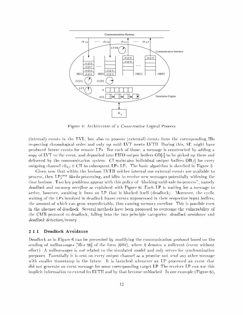
ulation would) the expected simulation time would be E[T async] = E[maxi=1::P (k Tstep;i)] > k� .We have limk!1;P!1 E[T sync]E[Tasync] � log(P ), saying that with increasing simulation size k, an asyn-chronous simulation could complete (at most) log(P ) times as fast as the synchronous simulation,and the maximum attainable speedup of any time stepped simulation is Plog(P ) . These results, how-ever, are a direct consequence of the exponential step execution time assumption, i.e. comparingthe expectation of the k-fold sum over the max of exponential random variates (synchronous) withthe expectation of the max over P k-stage Erlang random variates. For a step execution timeuniformly distributed over [l; u] we have limk!1;P!1 E[T sync]E[Tasync] � 2, or intuitively with T sync � k uand E[T async] � k (l+u)2 the ratio of synchronous to asynchronous �nishing times is 2(k u)(k (l+u)) � 2,i.e. constant. Therefore for a local event processing time distribution with �nite support the im-provement of an asynchronous strategy reduces to an amount independent of P .Certainly the model assumptions are far from what would be observed in real implementationson certain platforms, but the results might help to rank the two approaches at least from a statisticalviewpoint.2 \Classical" LP Simulation Protocols2.1 Conservative Logical ProcessesLP simulations following a conservative strategy date back to original works by Chandy and Misra[Chan 79] and Bryant [Brya 84], and are often referred to as the Chandy-Misra-Bryant (CMB)protocols. As described by [Misr 86], in CMB causality of events across LPs is preserved by sendingtimestamped (external) event messages of type hee@ti, where ee denotes the event and t is a copyof LVT of the sending LP at (@) the instant when the message was created and sent. t = ts(ee)is also called the timestamp of the event. A logical process following the conservative protocol(subsequently denoted by LPcons) is allowed to process safe events only, i.e. events up to a LVTfor which the LP has been guaranteed not to receive (external event) messages with LVT < t(timestamp \in the past"). Moreover, all events (internal and external) must be processed inchronological order. This guarantees that the message stream produced by an LPcons is in turn inchronological order, and a communication system (Figure 3) preserving the order of messages sentfrom LPconsi to LPconsj (FIFO) is su�cient to guarantee that no out of chronological order messagecan ever arrive in any LPconsi (necessary for correctness). A conservative LP simulation can thusbe seen as a set of all LPs LPcons = Sk LPconsk together with a set of directed, reliable, FIFOcommunication channels CH = Sk;i (k 6=i) chk;i = (LPk ;LPi) that constitute the Graph of LogicalProcesses GLPcons = (LP;CH). (It is important to note, that GLPcons has a static toplogy, whichcompared to optimistic protocols, prohibits dynamic (re-)scheduling of LPs in a set of physicalprocessors.)The communication interface CIcons of an LPcons on the input side maintains one input bu�erIB[i] and a channel (or link) clock CC[i] for every channel chi;k 2 CH pointing to LPconsk (Figure 4).IB[i] intermediately stores arriving messages in FIFO order, whereas CC[i] holds a copy of thetimestamp of the message at the head of IB[i]; initially CC[i] is set to zero. LVTH = miniCC[i]is the time horizon up until which LVT is allowed to progress by simulating internal or externalevents, since no external event can arrive with a timestamp smaller than LVTH. CI now triggersthe SE to conduct event processing just like a (sequential) event driven SE (Figure 1) based on11

Rk

e2 @ t1

e4 @ t2

e3 @ t7

e1 @ t9

e3 @ t3

e2 @ t5

e0 @ t0

e2 @ t0

e4 @ t0

CC[P]

Communication Interface

Simulation Engine

Communication System

IB[1]

CC[1]

IB[P] OB[1] OB[P]

LVT

LVTH

S

EVL

ch 1,k ch P,k ch k,1 ch k,P

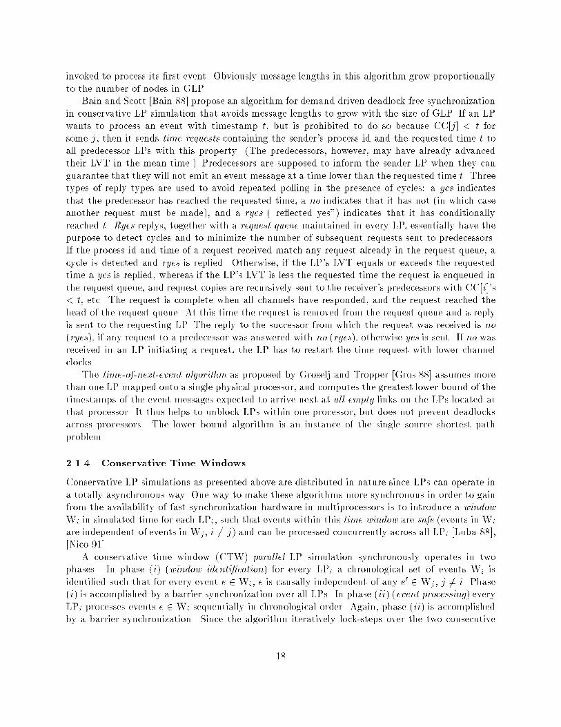
Figure 4: Architecture of a Conservative Logical Process(internal) events in the EVL, but also to process (external) events from the corresponding IBsrespecting chronological order and only up until LVT meets LVTH. During this, SE might haveproduced future events for remote LPs. For each of those, a message is constructed by adding acopy of LVT to the event, and deposited into FIFO output bu�ers OB[i] to be picked up there anddelivered by the communication system. CI maintains individual output bu�ers OB[i] for everyoutgoing channel chk;l 2 CH to subsequent LPs LPl. The basic algorithm is sketched in Figure 5.Given now that within the horizon LVTH neither internal nor external events are available toprocess, then LPconsk blocks processing, and idles to receive new messages potentially widening thetime horizon. Two key problems appear with this policy of \blocking-until-safe-to-process", namelydeadlock and memory over ow as explained with Figure 6: Each LP is waiting for a message toarrive, however, awaiting it from an LP that is blocked itself (deadlock). Moreover, the cyclicwaiting of the LPs involved in deadlock leaves events unprocessed in their respective input bu�ers,the amount of which can grow unpredictably, thus causing memory over ow. This is possible evenin the absence of deadlock. Several methods have been proposed to overcome the vulnerability ofthe CMB protocol to deadlock, falling into the two principle categories: deadlock avoidance anddeadlock detection/recory.2.1.1 Deadlock AvoidanceDeadlock as in Figure 6 can be prevented by modifying the communication protocol based on thesending of nullmessages [Misr 86] of the form h0@ti, where 0 denotes a nullevent (event withoute�ect). A nullmessages is not related to the simulated model and only serves for synchronizationpurposes. Essentially it is sent on every output channel as a promise not send any other messagewith smaller timestamp in the future. It is launched whenever an LP processed an event thatdid not generate an event message for some corresponding target LP. The receiver LP can use thisimplicit information to extend its LVTH and by that become unblocked. In our example (Figure 6),12

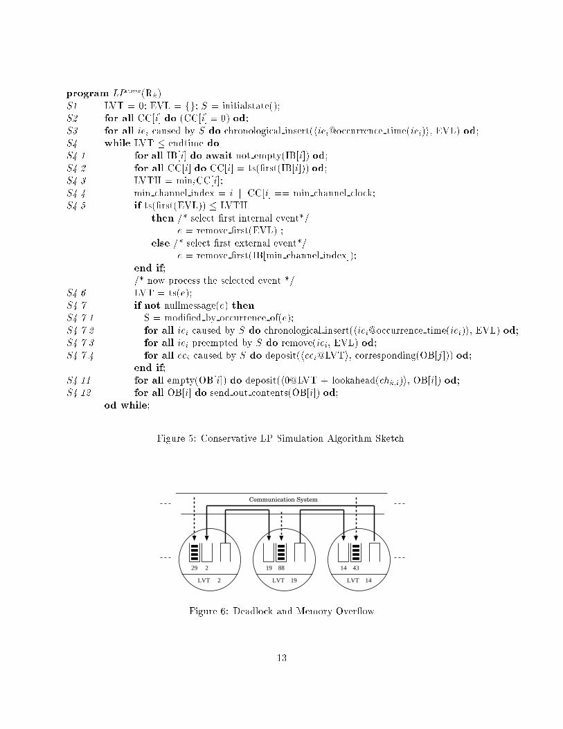
program LPcons(Rk)S1 LVT = 0; EVL = fg; S = initialstate();S2 for all CC[i] do (CC[i] = 0) od;S3 for all iei caused by S do chronological insert(hiei@occurrence time(iei)i, EVL) od;S4 while LVT � endtime doS4.1 for all IB[i] do await not empty(IB[i]) od;S4.2 for all CC[i] do CC[i] = ts(�rst(IB[i])) od;S4.3 LVTH = miniCC[i];S4.4 min channel index = i j CC[i] == min channel clock;S4.5 if ts(�rst(EVL)) � LVTHthen /* select �rst internal event*/e = remove �rst(EVL) ;else /* select �rst external event*/e = remove �rst(IB[min channel index]);end if;/* now process the selected event */S4.6 LVT = ts(e);S4.7 if not nullmessage(e) thenS4.7.1 S = modi�ed by occurrence of(e);S4.7.2 for all iei caused by S do chronological insert(hiei@occurrence time(iei)i, EVL) od;S4.7.3 for all iei preempted by S do remove(iei, EVL) od;S4.7.4 for all eei caused by S do deposit(heei@LVTi, corresponding(OB[j])) od;end if;S4.11 for all empty(OB[i]) do deposit(h0@LVT + lookahead(chk;i)i, OB[i]) od;S4.12 for all OB[i] do send out contents(OB[i]) od;od while; Figure 5: Conservative LP Simulation Algorithm Sketch.Communication System

29

LVT

2

2

19

LVT

88

19

14

LVT

43

14Figure 6: Deadlock and Memory Over ow13

after the LP in the middle would have broadcasted h0@19i to the neighboring LPs, both of themwould have chance to progress their LVT up until time 19, and in turn issue new event messagesexpanding the LVTHs of other LPs etc. The nullmessage based protocol can be guaranteed to bedeadlock free as long as there are no closed cycles of channels, for which a message traversing thiscycle cannot increment its timestamp. This implies, that simulation models whose event structurecannot be decomposed into regions such that for every directed channel cycle there is at least oneLP to put a nonzero time increment on traversing messages cannot be simulated using CMB withnullmessages.Although the protocol extension is straight-forward to implement, it can put a dramatic burdenof nullmessage overhead on the performance of the LP simulation. Optimizations of the protocolto reduce the frequency and amount of nullmessages, e.g. sending them only on demand (uponrequest), delayed until some timeout, or only when an LP becomes blocked have been proposed[Misr 86]. An approach where additional information (essentially the routing path as observedduring traversal) is attached to the nullmessage, the carrier nullmessage protocol [Cai 90] will beinvestigated in more detail later.One problem that still remains with conservative LPs is the determination of when it is safeto process an event. The degree to which LPs can look ahead and predict future events plays acritical role in the safety veri�cation and as a consequence for the performance of conservative LPsimulations. In the example in Figure 6, if the LP with LVT 19 could know that processing thenext event will certainly increment LVT to 22, then nullmessages h0@22i (so called lookahead of 3)could have been broadcasted as further improvement on the LVTH of the receivers.Lookahead must come directly from the underlying simulation model and enhances the pre-diction of future events, which is { as seen { necessary to determine when it is safe to process anevent. The ability to exploit lookahead from FCFS queueing network simulations was originallydemonstrated by Nicol [Nico 88], the basic idea being that the simulation of a job arriving at aFCFS queue will certainly increment LVT by the service time, which can already be determined,e.g. by random variate presampling, upon arrival since the number of queued jobs is known andpreemption is not possible.2.1.2 Example: Conservative LP Simulation of a PN with Model ParallelismTo demonstrate the development and parallel execution of an LP simulation consider again a simu-lation model described in terms of a PN as depicted in the Figure 7. Assume a physical system con-sisting of three machines, either being in operation or being maintained. The PN model comprisestwo places and two transitions with stochastic timing and balanced �ring delays (�(T1) � exp(0:5),�(T2) � exp(0:5)), i.e. time operating is approximately the same as time being maintained. Relatedto those �ring delays and the number of machines being represented by circulating tokens, a certainamount of model parallelism can be exploited when partitioning the net into two LPs, such that theindividual PN regions of LP1 and LP2 are: R1 = (fT1g; fP1g; f(P1;T1)g; �(T1) � exp(� = 0:5));and R2 = (fT2g; fP2g; f(P2;T2)g; �(T2) � exp(� = 0:5)):Let the future list [Nico 88], a sequence of exponentially distributed random �ring times (randomvariates), for T1 and T2 be as in the table of Figure 7. The sequential simulation would thensequence the variates according to their resulting scheduling in virtual time units when simulatingthe timed behavior of the PN as in Table 1. This sequencing stems from the policy of always usingthe next free variate from the future list to schedule the occurrence of the next event in EVL. In14

T2T1 P2P1

exp(τ1 = λ ) exp(τ2 = λ )

Future Lists for = 2λ

0.510.390.420.050.880.17

T2

0.370.170.220.340.930.65

T1

Simulation Engine 1

Region 1 Region 2

Simulation Engine 2

Figure 7: LP Simulation of a Trivial PN with Model ParallelismStep VT S EVL T0 0.00 (2,1) T1@0.17; T1@0.37; T2@0.51 |1 0.17 (1,2) T1@0.37; T2@0.51; T2@0.56 T12 0.37 (0,3) T2@0.51; T2@0.56; T2@0.79 T13 0.51 (1,2) T2@0.56; T1@0.73; T2@0.79 T24 0.56 (2,1) T1@0.73; T2@0.79; T1@0.90 T25 0.73 (1,2) T2@0.78; T2@0.79; T1@0.90 T1Table 1: Sequential DES of a PN with Model Parallelisman LP simulation scheme this sequencing is related to the protocol applied to maintain causalityamong the events.To explain model parallelism as requested by an LP simulation scheme, observe that the �ringof a scheduled transition (internal event) always generates an external event, namely a messagecarrying a token as the event description (tokenmessage), and a timestamp equal to the local virtualtime LVT of the sending LP. On the other hand, the receipt of an event message (external event)always causes a new internal event to the receiving LP, namely the scheduling of a new transition�ring in the local EVL. By just looking at the PN model and the variates sampled in the futurelist (Figure 7), we observe that the �rst occurrence of T1 and the �rst occurrence of T2 could besimulated in a time overlapped way.This is explained as follows (Figure 8): Both T1 and T2 have in�nite server �ring semantics, i.e.whenever a token arrives in P1 or P2, T1 (or T2) is enabled with a scheduled �ring at LVT plus thetransitions next future variate. There are constantly M = 3 tokens in the PN model, therefore themaximum degree of enabling is M for both T1 and T2. Considering now the initial state S = (2; 1)(two tokens in P1 and one in P2), one occurrence of T1 is scheduled for time tT1 = 0.17, and anotherone for t0T1 = 0.37. One occurrence of T2 is scheduled for time tT2 = 0.51. The next variate forT1 is 0.22, the one for T2 is 0.39. A token can be expected in P1 at min(0:51; 0:39; 0:42) = 39 atthe earliest, leading to a new (the third) scheduling of T1 at 0:39 + 0:22 = 0:61 at the earliest,maybe later. Consequently the �rst occurrence of T1 must be at t(T11) = 0.17, and the secondoccurence of T1 must be t(T12) = 0.37. The �rst occurrence of T2 can be either the one scheduled15

fl(T2,4) = 0.05

0.00 0.17 0.37 0.51 0.56 0.73 0.780.79

T1

T2

fl(T1,2) = 0.17

fl(T1,1) = 0.37

fl(T1,4) = 0.34

fl(T2,1) = 0.51

fl(T2,2) = 0.39

fl(T2,3) = 0.42

fl(T1,3) = 0.22 fl(T1,5) = 0.93

fl(T2,5) = 0.88

i-th variate from future list of T1fl(T1,i) = t

fl(T2,i) = t i-th variate from future list of T2

fl(T2,6) = 0.17

firing of T1, token move schedules T2

firing of T2, token move schedules T1

0.90Figure 8: Model Parallelism Observed in the PN executionat 0.51, or the one invoked by the �rst occurence of T1 at 0.17 + 0.39 = 0.56, or the one invokedby the second occurence of T1 at 0.37 + 0.42 = 0.78. Clearly, the �rst occurence of T2 must beat t(T21) = 0.51, and the second occurrence of T2 must be at t(T22) = 0:17 + 0:39 = 0:56, etc.Since T11 ! T22 with t(T21) < t(T22) and T21 ! T13 with t(T11) < t(T13), T11 and T21 do notinterfere with each other and can therefore be simulated independently (T1i ! T2j denotes thedirect scheduling causality of the i�th occurrence of T1 onto the j�th occurrence of T2).As was seen, the model that we consider in Figure 7 provides inherent model parallelism.In order to exploit this model parallelism in a CMB simulation, the PN model is decomposedinto two regions R1 and R2, which are assigned to two LPs LP1 and LP2, such that GLP=(fLP1;LP2g; fch1;2; ch2;1g), where the channels ch1;2 and ch2;1 are supposed to substitute the PNarcs (T1;P2) and (T2;P1) respectively. Both ch1;2 and ch2;1 carry messages containing tokensthat were generated by the �ring of a transition in a remote LP. Consequently, ch1;2 propagates amessage of the form m = h1;P2; ti from LP1 to LP2 on the occurrence of a �ring of T1, in orderto deposit 1 (�rst component of m) token into place P2 (second component of m) at time t (thirdcomponent). The timestamp t is produced as a copy of the LVT of LP1 at the instant of that �ringof T1, that produced the token.A CMB parallel execution of the LP simulation model developed above, since operating in asynchronous way in two phases (�rst simulate one event locally, then transmit messages), generatesthe trace in Table 2. In step 0, both LPs use precomputed random variates from their individualfuture lists and schedule events. In step 1, no event processing can happen due to LVTH = 0:0,LPs are blocked (see indication in B column. Generally in such a situation every LPi computes itslookahead la(chi;j) imposed on the individual outputchannels j. In the example we havela(chi;j) = min( (LVTi �mink=1::Si(stk)) ; mink=1::(M�Si) flk )where stk is the scheduled occurrence time of the k-th entry in EVL, flk is the k-th free variate inthe future list, and M is the maximum enabling degree (tokens in the PN model). For example, thelookahead in LP1 in the state of step 1 imposed on the channel to LP2 is la(ch1;2) = 0:17, whereasla(ch2;1) = 0:39. la is now attached to the LP's LVT, giving the timestamps for the nullmessage h 0;P2; 0.17 i sent from LP1 to LP2, and h 0; P1; 0.39 i sent from LP2 to LP1. The latter, when arrivingat LP1, unblocks the SE1, such that the �rst event out of EVL1 can be processed, generating the16

Step LP1 LP2IB LVT SP1 EVL OB B IB LVT SP2 EVL OB B0 | 0.00 2 T1@0.17;T1@0.37 | | 0.00 1 T2@0.51 |1 | 0.00 2 T1@0.17;T1@0.37 h 0; P2; 0.17 i � | 0.00 1 T2@0.51 h 0; P1; 0.39 i �2 h 0; P1; 0.39 i 0.17 1 T1@0.37 h 1; P2; 0.17 i h 0; P2; 0.17 i 0.17 1 T2@0.51 h 0; P1; 0.51 i �3 h 0; P1; 0.51 i 0.37 0 | h 1; P2; 0.37 i h 1; P2; 0.17 i 0.17 2 T2@0.51;T2@0.56 h 0; P1; 0.51 i �4 h 0; P1; 0.51 i 0.51 0 | h 0; P2; 0.73 i � h 1; P2; 0.37 i 0.37 3 T2@0.51;T2@0.56;T2@0.79 h 0; P1; 0.51 i �5 h 0; P1; 0.51 i 0.51 0 | h 0; P2; 0.73 i � h 0; P2; 0.73 i 0.51 2 T2@0.56;T2@1.79 h 1; P1; 0.51 i6 h 1; P1; 0.51 i 0.51 1 T1@0.73 h 0; P2; 0.73 i � h 0; P2; 0.73 i 0.56 1 T2@0.79 h 1; P1; 0.56 i7 h 1; P1; 0.56 i 0.56 2 T1@0.73;T1@0.90 h 0; P2; 0.73 i � h 0; P2; 0.73 i 0.73 1 T2@0.79 h 0; P1; 0.78 i �8 h 0; P1; 0.78 i 0.73 1 T1@0.90 h 1; P2; 0.73 i h 0; P2; 0.73 i 0.73 1 T2@0.79 h 0; P1; 0.78 i �Table 2: Parallel Conservative LP Simulation of a PN with Model Parallelismevent message h 1; P1; 0.17 i. This message, however, as received by LP2 still cannot unblock LP2since it carries the same timestamp as the previous nullmessage; also the local lookahead cannot beimproved and h 0; P1; 0.51 i is resent. It takes another iteration to �nally unblock LP2, which canthen process its �rst event in step 5, etc. It is easy seen from the example, that the CMB protocol(for the particular example) forces a `logical' barrier synchronization whenever the sequential DES(see trace in Table 1) switches from processing a T1 related event to a T2 related one and viceversa (at VT 0.17, 0.51, 0.73, etc.). In the diagram in Figure 8, this is at points where the arrowdenoting a token move from T1 (T2) to T2 (T1) has the opposite direction that the previous one.2.1.3 Deadlock Detection/RecoveryAn alternative to the Chandy-Misra-Bryant protocol avoiding nullmessages has also been proposedby Chandy and Misra [Chan 81], allowing deadlocks to occur, but providing a mechanism to detectit and recover from it. Their algorithm runs in two phases: (i) parallel phase, in which the simulationruns until it deadlocks, and (ii) phase interface, which initiates a computation allowing some LPto advance LVT. They prove, that in every parallel phase at least one event will be processedgenerating at least one event message, which will also be propagated before the next deadlock. Acentral controller is assumed in their algorithm, thus violating a distributed computing principle.To avoid a single resource (controller) to become a communication performance bottleneck duringdeadlock detection, any general distributed termination detection algorithm [Matt 87] or distributeddeadlock detection algorithm [Chan 83] could be used instead.In an algorithm described by Misra [Misr 86], a special message called marker circulates throughGLP to detect and correct deadlock. A cyclic path for traversing all chi;j 2 CH is precomputedand LPs are initially colored white. An LP that received the marker takes the color white and issupposed to route it along the cycle in �nite time. Once an LP has either received or sent an eventmessage since passing the marker, it turns to red. The marker identi�es deadlock if the last N LPsvisited were all white. Deadlock is properly detected as long as for any chi;j 2 CH all messagessent over chi;j arrive at LPj in the time order as sent by LPi. If the marker also carries the nextevent times of visited white LPs, it knows upon detection of deadlock the smallest next event timeas well as the LP in which this event is supposed to occur. To recover from deadlock, this LP is17

invoked to process its �rst event. Obviously message lengths in this algorithm grow proportionallyto the number of nodes in GLP.Bain and Scott [Bain 88] propose an algorithm for demand driven deadlock free synchronizationin conservative LP simulation that avoids message lengths to grow with the size of GLP. If an LPwants to process an event with timestamp t, but is prohibited to do so because CC[j] < t forsome j, then it sends time requests containing the sender's process id and the requested time t toall predecessor LPs with this property. (The predecessors, however, may have already advancedtheir LVT in the mean time.) Predecessors are supposed to inform the sender LP when they canguarantee that they will not emit an event message at a time lower than the requested time t. Threetypes of reply types are used to avoid repeated polling in the presence of cycles: a yes indicatesthat the predecessor has reached the requested time, a no indicates that it has not (in which caseanother request must be made), and a ryes (\re ected yes") indicates that it has conditionallyreached t. Ryes replys, together with a request queue maintained in every LP, essentially have thepurpose to detect cycles and to minimize the number of subsequent requests sent to predecessors.If the process id and time of a request received match any request already in the request queue, acycle is detected and ryes is replied. Otherwise, if the LP's LVT equals or exceeds the requestedtime a yes is replied, whereas if the LP's LVT is less the requested time the request is enqueued inthe request queue, and request copies are recursively sent to the receiver's predecessors with CC[i]'s< t, etc. The request is complete when all channels have responded, and the request reached thehead of the request queue. At this time the request is removed from the request queue and a replyis sent to the requesting LP. The reply to the successor from which the request was received is no(ryes), if any request to a predecessor was answered with no (ryes), otherwise yes is sent. If no wasreceived in an LP initiating a request, the LP has to restart the time request with lower channelclocks.The time-of-next-event algorithm as proposed by Groselj and Tropper [Gros 88] assumes morethan one LP mapped onto a single physical processor, and computes the greatest lower bound of thetimestamps of the event messages expected to arrive next at all empty links on the LPs located atthat processor. It thus helps to unblock LPs within one processor, but does not prevent deadlocksacross processors. The lower bound algorithm is an instance of the single source shortest pathproblem.2.1.4 Conservative Time WindowsConservative LP simulations as presented above are distributed in nature since LPs can operate ina totally asynchronous way. One way to make these algorithms more synchronous in order to gainfrom the availability of fast synchronization hardware in multiprocessors is to introduce a windowWi in simulated time for each LPi, such that events within this time window are safe (events in Wiare independent of events in Wj , i 6= j) and can be processed concurrently across all LPi [Luba 88],[Nico 91].A conservative time window (CTW) parallel LP simulation synchronously operates in twophases. In phase (i) (window identi�cation) for every LPi a chronological set of events Wi isidenti�ed such that for every event e 2 Wi, e is causally independent of any e0 2 Wj , j 6= i. Phase(i) is accomplished by a barrier synchronization over all LPs. In phase (ii) (event processing) everyLPi processes events e 2 Wi sequentially in chronological order. Again, phase (ii) is accomplishedby a barrier synchronization. Since the algorithm iteratively lock-steps over the two consecutive18

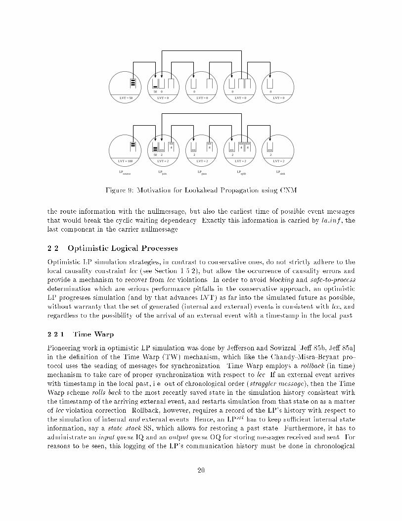
phases, the hope to gain speedup over a purely sequential DES heavily depends on the e�ciencyof the synchronization operation on the target architecture, but also on the event structure in thesimulation model. Di�erent windows will generally have di�erent cardinality of the covered eventset, maybe some windows will remain empty after the identi�cation phase for one cycle. In thiscase the corresponding LPs would idle for that cycle.A considerable overhead can be imposed on the algorithm by the identi�cation of when it issafe to process an event within LPi (window identi�cation phase). Lubachevsy [Luba 88] proposesto reduce the complexity of this operation by restricting the lag on the LP simulation, i.e. thedi�erence in occurrence time of events being processed concurrently is bounded from above bya know �nite constant (bounded lag protocol). By this restriction, and assuming a \reasonable"amount of dispersion of events in space and time, the execution of the algorithm on N processors inparallel will have one event processed in O(logN) time on average. An idealized message passingarchitecture with a tree-structured synchronization network supporting an e�cient realization ofthe bounded lag restriction is assumed for the analysis.2.1.5 The Carrier Null Message ProtocolAnother approach to reduce the overwhelming amount of null messages occuring with the CMBprotocol is to add more information to the null messages. The carrier null message protocol [Cai 90]uses nullmessages to advance CC[i]'s and acquire/propagate knowledge global to the participatingLPs, with the goal of improving the ability of lookahead to reduce the message tra�c.Indeed, good lookahead can reduce the number nullmessages as is motivated by the examplein Figure 9, where a source process produces objects in constant time intervals ! = 50. Thejoin, pass and split processes manipulate objects, consuming 2 time units per object. Eventu-ally objects are released from split into sink. For the example we have la(chi;j) = 2 8i; j 2fsource; join; pass; split; sinkg, (i 6= j), except la(chsource;join) = 50. After the �rst object releaseinto LPjoin, all LPs except LPsource are blocked, and therefore start propagating local lookaheadvia nullmessages. After the propagation of (overall) 4 nullmessages all LPs beyond LPsource haveprogressed LVT's and CC's to 2. It shall take further 96 nullmessages until LPjoin can make its�rst object manipulation, and after that another 100 for the second object, etc. If LPjoin couldhave learned that it had just waited for itself, it could have immediately simulated the externalevent (with VT 50). Besides the importance of the availability of global information within the LPs,the impact of lookahead onto LP simulation performance is now also easily seen: the smaller thelookahead in the successor LPs, the higher the communication overhead caused by nullmessages,the higher also the performance degrade.To generally realize such a waiting dependency across LPs the CNM protocol employs additionalnullmessages of type hc0; t;R, la:infi, where c0 is an identi�cation as a carrier nullmessage, t isthe timestamp, R is information about the travelling route of the message and la:inf is lookaheadinformation. Once LPjoin had received a carrier nullmessage with its id as source and sink in R,it can be sure (but only in the paricular example) not to receive an event message via that path,unless LPjoin itself had sent an event message along that path. So it can { without further waiting {after having received the �rst carrier nullmessage process the event message from LPsource, andthus increment the CC's and LVT's of all successors on the route in R considerably.Should there be any other \source"-like LP entering event messages into the waiting dependencyloop, the arguments above are no longer valid. For this case it is in fact not su�cient to only carry19

LVT = 0 LVT = 0LVT = 50

50

LVT = 0

0 0 0 0

50 2 2 2 2

LVT = 0

LVT = 2 LVT = 2LVT = 100 LVT = 2 LVT = 2

LPsource

LPjoin

LPpass

LPsplit

LPsink

4 4 44Figure 9: Motivation for Lookahead Propagation using CNMthe route information with the nullmessage, but also the earliest time of possible event messagesthat would break the cyclic waiting dependency. Exactly this information is carried by la:inf , thelast component in the carrier nullmessage.2.2 Optimistic Logical ProcessesOptimistic LP simulation strategies, in contrast to conservative ones, do not strictly adhere to thelocal causality constraint lcc (see Section 1.5.2), but allow the occurrence of causality errors andprovide a mechanism to recover from lcc violations. In order to avoid blocking and safe-to-processdetermination which are serious performance pitfalls in the conservative approach, an optimisticLP progresses simulation (and by that advances LVT) as far into the simulated future as possible,without warranty that the set of generated (internal and external) events is consistent with lcc, andregardless to the possibility of the arrival of an external event with a timestamp in the local past.2.2.1 Time WarpPioneering work in optimistic LP simulation was done by Je�erson and Sowizral [Je� 85b, Je� 85a]in the de�nition of the Time Warp (TW) mechanism, which like the Chandy-Misra-Bryant pro-tocol uses the sending of messages for synchronization. Time Warp employs a rollback (in time)mechanism to take care of proper synchronization with respect to lcc. If an external event arriveswith timestamp in the local past, i.e. out of chronological order (straggler message), then the TimeWarp scheme rolls back to the most recently saved state in the simulation history consistent withthe timestamp of the arriving external event, and restarts simulation from that state on as a matterof lcc violation correction. Rollback, however, requires a record of the LP's history with respect tothe simulation of internal and external events. Hence, an LPopt has to keep su�cient internal stateinformation, say a state stack SS, which allows for restoring a past state. Furthermore, it has toadministrate an input queue IQ and an output queue OQ for storing messages received and sent. Forreasons to be seen, this logging of the LP's communication history must be done in chronological20

Rk

Communication Interface

Simulation Engine

Communication System

IQ

IB OB

LVT

GVT

S

EVL

ch 1,k ch P,k ch k,1 ch k,P

SS

EVL

ie1 8 ie7 8 ie2 9 ei5 9

S0

0

S1

1

S2

1

S3

1

S4

2

S5

2

S6

3

S7

4

S8

4

S9

4

S10

5

S11

5

S12

6

EVL EVL EVL EVL EVL EVL

GVT LVT

3

ee1

4

ee3

4

ee5

6

ee2

9

ee1

GVT LVT

+ + + + +

OQ

3

ee4

4

ee1

6

ee6

7

ee1

GVT LVT

+ + + +

ee1 @ 5, +

ee2 @ 6, -

ee3 @ 7, +

ee1 @ 7, +

Figure 10: Architecture of an Optimistic Logical Processorder. Since the arrival of event messages in increasing time stamp order cannot be guaranteed, twodi�erent kinds of messages are necessary to implement the synchronization protocol: �rst the usualexternal event messages (m+ = hee@t;+i), (where again ee is the external event and t is a copy ofthe senders LVT at the sending instant) which will subsequently call positive messages. Opposed tothat are messages of type (m� = hee@t;�i) called negative- or antimessages, which are transmittedamong LPs as a request to annihilate the prematurely sent positive message containing ee, but forwhich it meanwhile turned out that it was computed based on a causally erroneous state.The basic architecture of an optimistic LP employing the Time Warp rollback mechanism isoutlined in Figure 10. External events are brought to some LPk by the communication system inmuch the same way as in the conservative protocol. Messages, however, are not required to arrivein the sending order (FIFO) in the optimistic protocol, which weakens the hardware requirementsfor executing Time Warp. Moreover, the separation of arrival streams is also not necessary, andso there is only a single IB and a single OB (assuming that the routing path can be deduced fromthe message itself). The communication related history of LPk is kept in IQ and OQ, whereas thestate related history is maintained in the SS data structure. All those together represent CIk ; SEkis an event driven simulation engine equivalent to the one in LPcons.The triggering of CI to SE is sketched with the basic algorithm for LPopt in Figure 11. TheLP mainly loops (S3) over four parts: (i) an input-synchronization to other LPs (S3.1), (ii) localevent processing (S3.2 { S3.8), (iii) the propagation of external e�ects (S3.9) and (iv) the (global)con�rmation of locally simulated events (S3.10 { S3.11). Part (ii) and (iii) are almost the same21

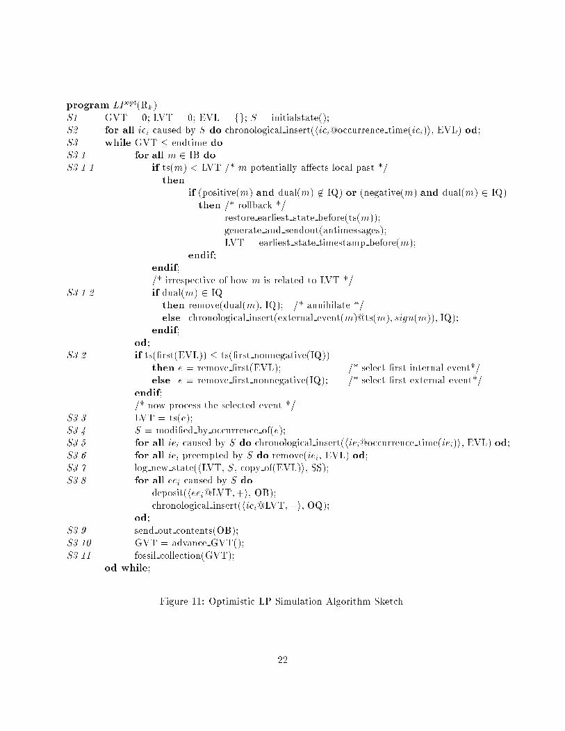
program LPopt(Rk)S1 GVT = 0; LVT = 0; EVL = fg; S = initialstate();S2 for all iei caused by S do chronological insert(hiei@occurrence time(iei)i, EVL) od;S3 while GVT � endtime doS3.1 for all m 2 IB doS3.1.1 if ts(m) < LVT /* m potentially a�ects local past */then if (positive(m) and dual(m) 62 IQ) or (negative(m) and dual(m) 2 IQ)then /* rollback */restore earliest state before(ts(m));generate and sendout(antimessages);LVT = earliest state timestamp before(m);endif;endif;/* irrespective of how m is related to LVT */S3.1.2 if dual(m) 2 IQthen remove(dual(m), IQ); /* annihilate */else chronological insert(external event(m)@ts(m); sign(m)), IQ);endif;od;S3.2 if ts(�rst(EVL)) � ts(�rst nonnegative(IQ))then e = remove �rst(EVL); /* select �rst internal event*/else e = remove �rst nonnegative(IQ); /* select �rst external event*/endif;/* now process the selected event */S3.3 LVT = ts(e);S3.4 S = modi�ed by occurrence of(e);S3.5 for all iei caused by S do chronological insert(hiei@occurrence time(iei)i, EVL) od;S3.6 for all iei preempted by S do remove(iei, EVL) od;S3.7 log new state(hLVT, S, copy of(EVL)i, SS);S3.8 for all eei caused by S dodeposit(heei@LVT;+i, OB);chronological insert(hiei@LVT;+i, OQ);od;S3.9 send out contents(OB);S3.10 GVT = advance GVT();S3.11 fossil collection(GVT);od while; Figure 11: Optimistic LP Simulation Algorithm Sketch.22

Arriving Message is of Type:

m+

timestamp(m) >= LVT

(in the local future)

timestamp(m) < LVT

(in the local past)

m

dual m exists in IQ

dual m does NOT exist

annihilate dual m_

_

_

chronological insert (m , IQ)_

+

dual m exists in IQ (not yet processed)

dual m does NOT exist

annihilate dual m

_

+

chronological insert (m , IQ)+

+

dual m exists in IQ

dual m does NOT exist

annihilate dual m_

_

chronological insert (m , IQ)_

+rollback

dual m exists in IQ (already processed)

dual m does NOT exist

annihilate dual m

_

+

chronological insert (m , IQ)+

+rollbackFigure 12: The Time Warp Message based Synchronization Mechanismas was seen with LPcons. The input synchronization (Rollback and Annihilation) and con�rmation(GVT) part however are the key mechanisms in optimistic LP simulation.2.2.2 Rollback and Annihilation MechanismsThe input synchronization of LPopt (rollback mechanism) relates arriving messages to the currentvalue of the LP's LVT and reacts accordingly (see Figure 12). A message a�ecting the LP's \localfuture" is moved from the IB to the IQ respecting the timestamp order, and the encoded externalevent will be processed as soon as LVT advances to that time. hee3@7;+i in the IB in Figure 10is an example of such an unproblematic message (LVT = 6). A message timestamped in the \localpast" however is an indicator of a causality violation due to tentative event processing. The rollbackmechanism (S3.1.1 ) in this case restores the most recent lcc-consistent state, by reconstructing Sand EVL in the simulation engine from copies attached to the SS in the communication interface.Also LVT is warped back to the timestamp of the straggler message. This so far has compensatedthe local e�ects of the lcc violation; the external e�ects are annihilated by sending an antimessagefor all previously sent outputmessages (in the example hee6@6;�i and hee1@7;�i are generatedand sent out, while at the same time hee6@6;+i and hee1@7;+i are removed from OQ). Finally, ifa negative message is received (e.g. hee2@6;�i) it is used to annihilate the dual positive message(hee2@6;+i) in the local IQ. Two cases for the negative messages must be distinguished: (i) If thedual positive message is present in the receiver IQ, then this entry is deleted as an annihilation.This can be easily done if the positive message has not yet been processed, but requires rollback ifit was. (ii), if a dual positive message is not present (this case can only arise if the communication23

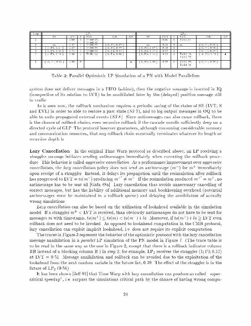
Step LP1 LP2IB LVT S EVL OB RB IB LVT S EVL OB RB0 | 0.00 2 T1@0.17;T1@0.37 | | 0.00 1 T2@0.51 |1 | 0.17 1 T1@0.37 h 1; P2; 0.17 i | 0.51 0 | h 1; P1; 0.51 i2 h 1; P1; 0.51 i 0.37 1 T1@0.73 h 1; P2; 0.37 i h 1; P2; 0.17 i 0.56 0 | h 1; P1; 0.56 i3 h 1; P1; 0.56 i 0.73 1 T1@0.90 h 1; P2; 0.73 i h 1; P2; 0.37 i 0.79 0 | h 1; P1; 0.79 i4 h 1; P1; 0.79 i 0.90 1 T1@1.72 h 1; P2; 0.90 i h 1; P2; 0.73 i 0.73 2 T2@0.78;T2@0.79 h -1; P1; 0.79 i �5 h -1; P1; 0.79 i 0.90 0 | | � h 1; P2; 0.90 i 0.78 2 T2@0.79;T2@1.78 h 1; P1; 0.78 iTable 3: Parallel Optimistic LP Simulation of a PN with Model Parallelismsystem does not deliver messages in a FIFO fashion), then the negative message is inserted in IQ(irrespective of its relation to LVT) to be annihilated later by the (delayed) positive message stillin tra�c.As is seen now, the rollback mechanism requires a periodic saving of the states of SE (LVT, Sand EVL) in order to able to restore a past state (S3.7 ), and to log output messages in OQ to beable to undo propagated external events (S3.8 ). Since antimessages can also cause rollback, thereis the chance of rollback chains, even recursive rollback if the cascade unrolls su�ciently deep on adirected cycle of GLP. The protocol however guarantees, although consuming considerable memoryand communication resources, that any rollback chain eventually terminates whatever its length orrecursive depth is.Lazy Cancellation In the original Time Warp protocol as described above, an LP receiving astraggler message initiates sending antimessages immediately when executing the rollback proce-dure. This behavior is called aggressive cancellation. As a performance improvement over aggressivecancellation, the lazy cancellation policy does not send an antimessage (m�) for m+ immediatelyupon receipt of a straggler. Instead, it delays its propagation until the resimulation after rollbackhas progressed to LVT = ts(m+) producing m+0 6= m+. If the resimulation produced m+0 = m+, noantimessage has to be sent all [Gafn 88a]. Lazy cancellation thus avoids unnecessary cancelling ofcorrect messages, but has the liability of additional memory and bookkeeping overhead (potentialantimessages must be maintained in a rollback queue) and delaying the annihilation of actuallywrong simulations.Lazy cancellation can also be based on the utilization of lookahead available in the simulationmodel. If a stragglerm+ < LVT is received, than obviously antimessages do not have to be sent formessages m with timestamp, ts(m+) � ts(m) < ts(m+)+ la. Moreover, if ts(m+)+ la � LVT evenrollback does not need to be invoked. As opposed to lookahead computation in the CMB protocol,lazy cancellation can exploit implicit lookahead, i.e. does not require its explicit computation.The traces in Figure 3 represent the behavior of the optimistic protocol with the lazy cancellationmessage annihilation in a parallel LP simulation of the PN model in Figure 7. (The trace table isto be read in the same way as the one in Figure 2, except that there is a rollback indicator columnRB instead of a blocking column B.) In step 2, for example, LP2 receives the straggler h1; P1; 0:17iat LVT = 0.51. Message annihilation and rollback can be avoided due to the exploitation of thelookahead from the next random variate in the future list, 0.39. The e�ect of the straggler is in thefuture of LP2 (0.56).It has been shown [Je� 91] that Time Warp with lazy cancellation can produce so called \super-critical speedup", i.e. surpass the simulations critical path by the chance of having wrong compu-24

tations produce correct results. By immediately discarding rolled back computations this chance islost for the aggressive cancellation policy. A performance comparison of the two, however, is relatedto the simulation model. Analysis by Reiher and Fujimoto [Reih 90] shows that lazy cancellationcan arbitrarily outperform aggressive cancellation and vice versa, i.e. one can construct extremecases for lazy and aggressive cancellation such that if one protocol executes in � time using Nprocessors, the other uses �N time. Nevertheless, empirical evidence is reported \slightly" in favorof lazy cancellation for certain simulation applications.Lazy Reevaluation Much like lazy cancellation delays the annihilation of external e�ects uponreceiving a straggler at LVT, lazy re-evaluation delays discarding entries on the state stack SS.Should the recomputation after rollback to time t < LVT reach a state that exactly matches onelogged in SS and the IQ is the same as the one at that state, then immediately jump forward toLVT, the time before rollback occured. Thus, lazy reevaluation prevents from the unnecessaryrecomputation of correct states and is therefore promising in simulation models where events donot modify states (\read-only" events). A serious liability of this optimization is again additionalmemory and bookkeeping overhead, but also (and mainly) the considerable complication of theTime Warp code [Fuji 90]. To verify equivalence of IQ's the protocol must draw and log copies ofthe IQ in every state saving step (S3.7 ). In a weaker lazy re-evaluation strategy one could allowjumping forward only if no message has arrived since rollback.Lazy Rollback The di�erence of virtual time in between the straggler m�, ts(m�), and its actuale�ect at time ts(m�) + la(ee) � LVT can again be overjumped, saving the computation time forthe resimulation of events in between [ts(m�); ts(m�) + la(ee)). la(ee) is the lookahead imposed bythe external event carried by m�.Breaking/Preventing Rollback Chains Besides the postponing of erroneous message andstate annihilation until it turns out that they are not reproduced in the repeated simulation, othertechniques have been studied to break cascades of rollbacks as early as possible. Prakash andSubramanian [Prak 91], comparable to the carrier null message approach, attach a limited amountof state information to messages to prevent recursive rollbacks in cyclic GLPs. This informationallows LPs to �lter out messages based on preempted (obsolete) states to be eventually annihilatedby chasing antimessages currently in transit. Related to the (conservative) bounded lag algorithm,Lubachevsky, Shwartz and Weiss have developed a �ltered rollback protocol [Luba 91] that allowsoptimistically crossing the lag bound, but only up to a time window upper edge. Causality violationscan only a�ect the time period in between the window edge and the lag bound, thus limiting(the relative) length of rollback chains. The SRADS protocol by Dickens and Reynolds [Dick 90],although allowing optimistic simulation progression, prohibits the propagation of uncommittedevents to other LPs. Therefore, rollback can only be local to some LP and cascades of rollbackcan never occur. Madisetti, Walrand and Messerschmitt with their protocol called Wolf-calls freezethe spatial spreading of uncommitted events in so called spheres of in uence W (LPi; �), de�nedas the set of LPs that can be in uenced by a message from LPi at time ts(m) + � respectingcomputation times a and communication times b. The Wolf algorithm ensures that the e�ects ofan uncommitted event generated by LPi are limited to a sphere of a computable (or selectable)radius around LPi, and the number of broadcasts necessary for a complete annihilation within the25

sphere is bounded by a computable (or chooseable) number of steps B (B being provably smallerthan for the standard Time Warp protocol).2.2.3 Optimistic Time WindowsA similar idea of \limiting the optimism" to overcome rollback overhead potentials is to advancecomputations by \windows" moving over simulated time. In the original work of Sokol, Briscoe andWieland [Soko 88], the moving time window (MTW) protocol, neither internal nor external eventse with ts(e) > t+� are allowed to be simulated in the time window [t; t+�), but are postponed forthe next time window [t+�; t+2�). Two events e and e0 timestamped ts(e) and ts(e0) respectivelytherefore can only be simulated in parallel i� j ts(e)�ts(e0) j< �. Naturally, the protocol is in favorof simulation models with a low variation of event occurrence distances relative to the window size.Compared to a time-stepped simulation, MTW does not await the completion of all events e witht � ts(e) < t+� which would cause idle processors at the end of each time window, but invokes anattempt to move the window as soon as the number of events to be executed falls below a certainthreshold. In order to keep moving the time window, LPs are polled for the timestamp of theirearliest next event ti(e) (polling takes place simultaneously with event processing) and the windowis advanced to mini ti(e);mini ti(e)+�. (The next section will show the equivalence of the windowlower edge determination to GVT computation.) Obviously the advantage of MTW and relatedprotocols is the potential e�ective implementation as a parallel LP simulation, either on a SIMDarchitecture or in a MIMD environment where the reduction operation mini ti(e) can be computedutilizing synchronization hardware. Points of criticism are the assumption of approximately uniformdistribution of event occurrence times in space and the ignorance with respect to potentially \good"optimism beyond the upper window edge. Furthermore, a natural di�culty is the determination ofthe � admitting enough events to make the simulation e�cient.The latter is addressed with the adaptive Time Warp concurrency control algorithm (ATW)proposed by Ball and Hyot [Ball 90], allowing the window size �(t) be adapted at any point t insimulation time. ATW aims to temporarily suspend event processing if it has observed a certainamount of lcc violations in the past. In this case the LP would conclude that it progresses LVTtoo fast compared to the predecessor LPs and would therefore stop LVT advancement for a timeperiod called the blocking window (BW). BW is determined based on the minimum of a functiondescribing wasted computation in terms of time spent in a (conservatively) blocked mode, or a faultrecovery mode as induced by the Time Warp rollback mechanism.2.2.4 The Limited Memory DilemmaAll arguments on the execution of the Time Warp protocol so far assumed the availability of asu�cient amount of free memory to record internal and external e�ect history for pending rollbacks,and all arguments were related to the time complexity. Indeed, Time Warp with certain memorymanagement strategies to be described in the sequel can be proven to work correctly when executedwith O(M seq) memory, whereM seq is the number of memory locations utilized by the correspondingsequential DES. Opposed to that, the CMB protocol may require O(kM seq) space, but may alsouse less storage than sequential simulation, depending on the simulation model ( it can even beproven that simulation models exist such that the space complexity of CMB is O((M seq)k)). TimeWarp always consumes more memory than sequential simulation [Lin 91], and a memory limitationimposes a performance decrease on Time Warp: providing just the minimum of memory necessary26

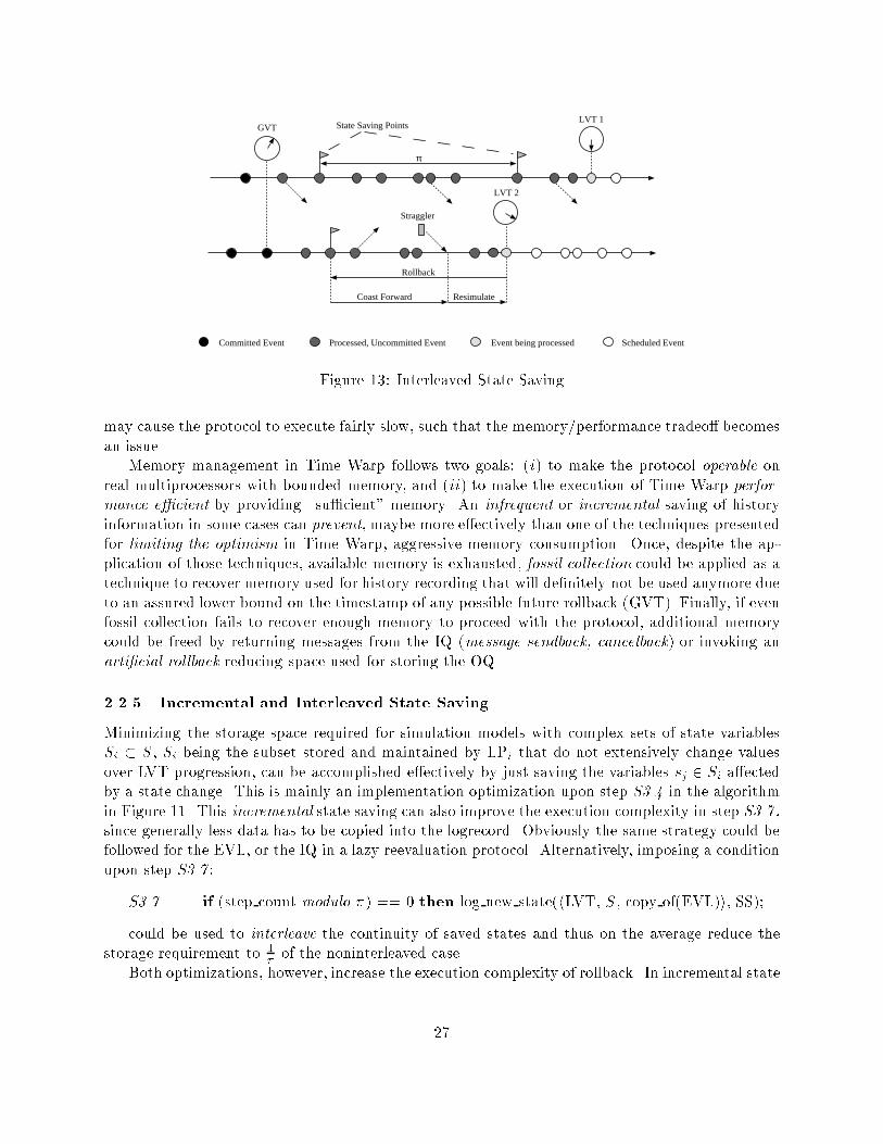
GVTLVT 1

LVT 2

Straggler

State Saving Points

Rollback

Coast Forward Resimulate

Committed Event Processed, Uncommitted Event Event being processed Scheduled Event

π

Figure 13: Interleaved State Savingmay cause the protocol to execute fairly slow, such that the memory/performance tradeo� becomesan issue.Memory management in Time Warp follows two goals: (i) to make the protocol operable onreal multiprocessors with bounded memory, and (ii) to make the execution of Time Warp perfor-mance e�cient by providing \su�cient" memory. An infrequent or incremental saving of historyinformation in some cases can prevent, maybe more e�ectively than one of the techniques presentedfor limiting the optimism in Time Warp, aggressive memory consumption. Once, despite the ap-plication of those techniques, available memory is exhausted, fossil collection could be applied as atechnique to recover memory used for history recording that will de�nitely not be used anymore dueto an assured lower bound on the timestamp of any possible future rollback (GVT). Finally, if evenfossil collection fails to recover enough memory to proceed with the protocol, additional memorycould be freed by returning messages from the IQ (message sendback, cancelback) or invoking anarti�cial rollback reducing space used for storing the OQ.2.2.5 Incremental and Interleaved State SavingMinimizing the storage space required for simulation models with complex sets of state variablesSi � S, Si being the subset stored and maintained by LPi that do not extensively change valuesover LVT progression, can be accomplished e�ectively by just saving the variables sj 2 Si a�ectedby a state change. This is mainly an implementation optimization upon step S3.4 in the algorithmin Figure 11. This incremental state saving can also improve the execution complexity in step S3.7 ,since generally less data has to be copied into the logrecord. Obviously the same strategy could befollowed for the EVL, or the IQ in a lazy reevaluation protocol. Alternatively, imposing a conditionupon step S3.7 :S3.7 if (step count modulo �) == 0 then log new state(hLVT, S, copy of(EVL)i, SS);could be used to interleave the continuity of saved states and thus on the average reduce thestorage requirement to 1� of the noninterleaved case.Both optimizations, however, increase the execution complexity of rollback. In incremental state27

saving protocols, desired states have to be reconstructed from increments following back a pathfurther into the simulated past than required by rollback itself. The same is true for interleavedstate saving, where the most recent saved state older than the straggler must be searched for, areexecution up until the timestamp of the straggler (coast forward) must be started which is a clearwaste of CPU cycles since it just reproduces states that have already been computed but werenot saved, and �nally the straggler integration and usual reexecution are necessary (Figure 13).The tradeo� between state saving costs and the coast forward overhead has been studied (asreported by [Nico 94] in reference to Lin and Lazowska) based on expected event processing time(� = E[exec(e)]) and state saving costs (�), giving an optimal interleaving factor �� asbq(�� 1)�c < �� < dq(2�+ 1)�ewhere � is the average number of rollbacks with � = 1 and � = �� . The result expresses that anoverestimation of �� is more severe to performance than an underestimation by the same (absolute)amount. In a study of the optimal checkpointing interval explicitly considering state saving andrestoration costs while assuming � does neither a�ect the number of rollbacks nor the number ofrolled back events in [Lin 93], an algorithm is developed that, integrated into the protocol, \on-the- y", within a few iterations, automatically adjusts � to ��. It has been shown that some �,though increasing the rollback overhead, can reduce overall execution time.2.2.6 Fossil CollectionOpposed to techniques that reclaim memory temporarily used for storing events and messagesrelated to the future of some LP, fossil collection aims to return space used by history records thatwill no longer be used by the rollback synchronization mechanism. To assure from which state inthe history (and back) computations can be considered fully committed, the determination of thevalue of global virtual time (GVT) is necessary.Consider the tuple �i(T ) = (LVTi(T ); IQi(T ); SSi(T );OQi(T ))to be a local snapshot of LPi at real time T , i.e. LVT, IQi is the input queue as seen by anexternal observer at real time T , etc., and �(T ) = SNi=1�i(T ) [ CS(T ) be the global snapshot ofGLP. Further let LVTi(T ) be the local virtual time in LPi, i.e. the timestamp of the event beingprocessed at the observation instant T , and UMi;j(T ) the set of external events imposed by LPiupon LPj encoded as messages m in the snapshot �. This means m is either in transit on channelchi;j in CS or stored in some IQj , but not yet processed at time T . Then the GVT at real time Tis de�ned to be: GVT(T ) = min(mini LVTi(T ); mini;j;m2UMi;j(T ) ts(m))It should be clear even by intuition, that at any (real time) T , GVT(T ) represents the maximumlower bound to which any rollback could ever backdate LVTi (8i). An obvious consequence is thatany processed event e with ts(e) < GVT(T ) can never (at no instant T ) be rolled back, and cantherefore be considered as (irrevocably) committed [Lin 91] (Figure 13). Further consequences (forall LPi) are that: 28

(i) messagesm 2 IQi with ts(m) � GVT(T ), as well as messagesm 2 OQi with ts(m) � GVT(T )are obsolete and can be discarded (from IQ, OQ) after real time T .(ii) state variables s 2 Si stored in SSi as with ts(s) � GVT(T ) are obsolete and can be discardedafter real time T .Making use of these possibilities, i.e. getting rid of external event history according to (i) andof internal event history according to (ii) that is no longer needed to reclaim memory space is theidea behind fossil collection. It is called as a procedure in the abstracted Time Warp algorithm(Figure 11) in step S3.11 . The idea of reclaiming memory for history earlier than GVT is alsoexpressed in Figure 10, which shows IQ and OQ sections for entries with timestamp later thanGVT only, and copies of EVL in SS if not older than GVT (also the rest of SS beyond GVT couldbe purged as irrelevant for Time Warp, but we assume here that the state trace is required for apost-simulation analysis).Generally, a combination of fossil collection with any of the incremental/interleaved state savingschemes is recommended. Related to interleaving, however, rollback might be induced to eventsbeyond the momentary committed GVT, with an average overhead directly proportional �. Notonly that the interleaving of state recording is prohibiting fossil collection for states timestampedin the gap between GVT and the most recent saved state chronologically before GVT, it is alsocontraproductive to GVT computation which is comparably more expensive than state saving aswill be seen soon.2.2.7 Freeing Memory by Returning MessagesPrevious strategies (interleaved, incremental state saving as well as fossil collection) are merelyable to reduce the chance of memory exhaustion, but cannot actually prevent such situations fromoccurring. In cases where memory is already completely allocated, only additional techniques,mostly based on returning messages to senders or arti�cially initiating rollback, can help to escapefrom deadlocks due to waiting for free memory:Message Sendback The �rst approach to recover from memory over ow in Time Warp wasproposed by the message sendback mechanism by Je�erson [Je� 85a]. Here, whenever the systemruns out of memory on the occasion of an arriving message, part or all af the space used for savingthe input history is used to recover free memory by returning unprocessed input messages (notnecessarily including the one just received) back to the sender and relocating the freed (local)memory. By intuition, input messages with the highest send timestamps are returned �rst, sinceit is more likely that they carry incorrect information compared to \older" input messages, andsince the annihilation of their e�ects can be expected not to disperse as much in virtual time,thus restriciting annihilation in uence spheres. Related to the original de�nition of the TimeWarp protocol which distinguishes the send time (ST) and receive time (RT) (ST(m) � RT(m)) ofmessages, only messages with ST(m) > LVT (local future messages) are considered for returning.An indirect e�ect of the sendback could also be storage release in remote LPs due to annihilationof messages triggered by the original sender's rollback procedure.Gafni's Protocol In a message tra�c study of aggressive and lazy cancellation, Gafni [Gafn 88b]notes that past (RT(m) < GVT) and present messages (ST(m) < GVT < RT(m)) and events29

accumulate in IQ, OQ, SS for the two annihilation mechanisms at the same rate, pointing out alsothe interweaving of messages and events in memory consumption. Past messages and events canbe fossil collected as soon as a new value of GVT is available. The amount of \present" messagesand events present in LPi re ects the di�erence of LVTi to the global GVT directly expressingthe asynchrony or \imbalance" of LVT progression. This fact gives an intuitive explanation of themessage sendback's attempt to balance LVT progression across LPs, i.e. intentionally rollback thoseLPs that have progressed LVT ahead of others. Gafni, considering this asynchrony to be exactlythe source from which Time Warp can gain real execution speedup, states that LVT progressionbalancing is does not solve the storage over ow problem. His algorithm reclaims memory byrelocating space used for saving the input or state or output history in the following way: Whetherthe over ow condition is raised by an arriving input message, the request to log a new state or thecreation of a new output message, the element (message or event) with the largest timestamp isselected irrespective of its type.� If it is an output message, a corresponding antimessage is sent, the element is removed fromOQ and the state before sending the original message is restored. The antimessage arrivingat the receiver will �nd its annihilation partner in the receiver's IQ upon arrival (at least inFIFO CSs), so memory is also reclaimed in the receiver LP.� If it is an input message, it is removed from IQ and returned to the original sender to beannihilated with its dual in the OQ, perhaps invoking rollback there. Again also the receiverLP relocates memory.� If it is a state in SS, it is discarded (and will be recomputed in case of local rollback).The desirable property of both message sendback and Gafni's protocol is that LPs that ranout of memory can be relieved without shifting the over ow condition to another LP. So, given acertain minimum but limited amount of memory, both protocols make Time Warp \operable".Cancelback An LP simulation memory management scheme is considered to be storage optimali� it consumes O(M seq) constant bounded memory [Lin 91]. The worst case space complexity ofGafni's protocol is O(NM seq) = O(N2) (irrespective of whether memory is shared or distributed),the reason for this being that it can only cancel elements within the individual LPs. Cancelbackis the �rst optimal memory management protocol [Je� 90], and was developed targeting TimeWarp implementations on shared memory systems. As opposed to Gafni's protocol, in Cancelbackelements can be canceled in any LPi (not necessarily in the one that observed memory over ow),whereas the element selection scheme is the same. Cancelback thus allows to selectively reclaimthose memory spaces that are used for the very most recent (globally seen) input-, state- or output-history records, whichever LP maintains this data. An obvious implementation of Cancelback istherefore for shared memory environments and making use of system level interrupts. A Markovchain model of Cancelback [Akyi 93] predicting speedup as the amount of available memory beyondM seq is varied, revealed that even with small fractions of additional memory the protocol performsabout as well as with unlimited memory. The model assumes totally symmetric workload and aconstant number of messages, but is veri�ed with empirical observations.30

Arti�cial Rollback Although Cancelback theoretically solves the memory management dilemmaof Time Warp since it produces correct simulations in real, limited memory environments with thesame order of storage requirement as the sequential DES, it has been criticized for its implemen-tation not being straightforward, especially in distributed memory environments. Lin [Lin 91]describes a Time Warp management scheme that is in turn memory optimal (there exists a sharedmemory implementation of Time Warp with space complexity O(M seq) 1), but has a simpler im-plementation. Lin's protocol is called arti�cial rollback for provoking the rollback procedure notonly for the purpose of lcc-violation restoration, but also for its side e�ect of reclaiming memory(since rollback as such does not a�ect operational correctness of Time Warp, it can also be invokedarti�cially, i.e. even in the absence of a straggler). Equivalent to Cancelback in e�ect (cancellingan element generated by LPj from IQi is equivalent to a rollback in LPj , whereas cancelling anelement from OQi or SSi is equivalent to a rollback in LPi), arti�cial rollback has a simpler im-plementation since the rollback procedure already available can be used together with an arti�cialrollback trigger causing only very little overhead. Determining, however, in which LPi to invokearti�cial rollback, to what LVT to rollback and at what instant of real time T to trigger it is nottrivial (except the triggering, which can be related to the over ow condition and the failure of fossilcollection). In the implementation proposed by Lin and Preiss [Lin 91], the two other issues arecoupled to a processor scheduling policy in order to guarantee a certain amount of free memory(called salvage parameter in [Nico 94]), while following the \cancel-furthest-ahead" principle.Adaptive Memory Management The adaptive memory management (AMM) scheme pro-posed by Das and Fujimoto [Das 94] attempts a combination of controling optimism in Time Warpand an automatic adjustment of the amount of memory in order to optimize fossil collection, Can-celback and rollback overheads. Analytical performance models of Time Warp with Cancelback[Akyi 93] for homogeneous (arti�cial) workloads have shown that at a certain amount of availablefree memory fossil collection is su�cient to allocate enough memory. With a decreasing amountof available memory, absolute execution performance decreases due to more frequent cancelbacksuntil it becomes frozen at some point. Strong empirical evidence has been given as a support tothis analytical observations. The motivation now for an adaptive mechanism to control memory istwofold: (i) absolute performance is supposed to have negative increments after reducing memoryeven further. Indeed, one would like to run Time Warp in the area of the \knee-point" of abso-lute performance. A successive adaptation to that performance optimal point is desired. (ii) thelocation of the knee might vary during the course of simulation due to the underlying simulationmodel. A runtime adaptation to follow movements of the knee is desired.The AMM protocol for automatic adjustment of available storage uses a memory ow modelthat divides the available (limited) memory space M into three \pools", M = M c +Muc +Mf .M c is the set of all memory locations used to store committed elements (t(e) � GVT), Muc is itsanalogy for uncommitted events (in IQ, OQ, or SS with t(e) > GVT) and Mf holds temporarilyunused (free) memory. The behavior of Time Warp can now be described in terms of ows of(�xed sized) memory bu�ers (able to record one message or event for simplicity) from one poolinto the other (Figure 14): Free memory must be allocated for every message created/sent, everystate logged or any future event scheduled, causing bu�er moves fromMf to Muc. Fossil collection1For implementations in distributed memory environments, Time Warp with arti�cial rollback cannot guarantee aspace complexity of O(Mseq). Cancelback and Arti�cial Rollback in achieving the sequential DES storage complexitybound rely on the availability of a global, shared pool of (free) memory.31

free memory

committed

uncommitted

processed unprocessed

GVT LVTGVT rollback

process event

fossil collection

GVT progression

- create and send message

- schedule event

- log state

message

annihilation

(cancelback)Figure 14: \Flow of bu�ers" in the AMM protocolon the other hand returns bu�ers from M c as invoked upon exhaustion of Mf , whereas M c isbeing supplied by the progression of GVT. Bu�ers move from Muc to Mf with each messageannihilation, either incurred by rollback or by Cancelback. A Cancelback cycle is de�ned by twoconsecutive invocations of cancelback. A cycle starts where Cancelback was called due to failure offossil collection to reclaim memory; at this point there are no bu�ers in M c. Progression of LVTwill move bu�ers toMuc, rollback of LVT will occasionally return free memory, progression of GVTwill deposit into M c to be depleted again by fossil collection, but tendentially the free pool will bedrained, thus necessitating a new cancelback.Time Warp can now be controlled by two (mutually dependent) parameters: (i) �, the amount ofprocessed but uncommitted bu�ers left behind after cancelback, as a parameter to control optimism;and (ii) �, the amount fo bu�ers freed by Cancelback, as a parameter to control the cycle length.Obviously, � has to be chosen small enough to avoid rollback thrashing and overly aggressivememory consumption, but not too small in order to prevent rollbacks of states that are most likelyto be con�rmed (events on the critical path). � should be chosen in such a way as to minimize theoverhead caused by unnecessary frequent cancelback (and fossil collection) calls. The AMM protocolnow by monitoring the Time Warp execution behavior during one cycle, attempts to simultaneouslyminimize the values of � and �, but respecting the constraints above. It assumes Cancelback (andfossil collection) overhead to be directly proportional to the Cancelback invocation frequency. Let%Muc = ecommittedNTprocess �%FC be the rate of growth ofMuc, where ecommitted is the fraction of processedevents also committed during the last cycle, Tprocess is the average (real) time to process an eventand %FC is the rate of depletion of Muc due to fossil collection. (Estimates for the right hand sideare generated from monitoring the simulation execution.) � is then approximated by� = (Tcycle � TCB;FC)%Mucwhere TCB;FC is the overhead incurred by Cancelback and fossil collection in real time units,and Tcycle is the current invocation interval. Indeed, � is a parameter to control the upper tolerablebound for the progression of LVT. To set � appropriately, AMM records by a marking mechanismwhether an event was rolled-back by Cancelback. A global (across all LPs) counting mechanism letsAMM determine the number #(ecp) of events that should not have been rolled back by Cancelback,32

since they were located on the critical path, and by that causing a de�nitive performance degrade2.Starting now with a high parameter value for � (which will give an observation #(ecp) ' 0), � iscontinuously reduced as long as #(ecp) remains negligible. Rollback thrashing is explicitly tackledby a third mechanism that monitors ecommitted and reduces � and � to their halves when thedecrease of ecommitted hits a prede�ned threshold.Experiments with the AMM protcol have shown that both the claimed needs can be achieved:Limiting optimism in Time Warp indirectly by controlling the rate of drain of free memory can beaccomplished e�ectively by a dynamically adaptive mechanism. AMM adapts this rate towards theperformance knee-point automatically, and adjusts it to follow dynamical movements of that pointdue to workloads varying (linearly) over time.2.2.8 Algorithms for GVT ComputationSo far, global virtual time has been assumed to be available at any instant of real time T in anyLPi, e.g. for fossil collection (S3.11 ) or in the simulation stopping criterion (S3 ). The de�nition ofGVT(T ) has been given in Section 2.2.6. An essential property of GVT(T ) not mentioned yet isthat it is nondecreasing over (real time) T and therefore can guarantee that Time Warp eventuallyprogresses the simulation by committing intermediate simulation work. E�cient algorithms tocompute GVT therefore are another foundational issue to make Time Warp \operable".The computation of GVT(T ) (S3.10 ) generally is hard, such that in practice only estimatesdGVT(T ) � GVT(T ) are attempted. Estimates dGVT(T ), however, (as a necessity to be practicallyuseful) are guaranteed to not overestimate the actual GVT(T ) and to eventually improve pastestimates.GVT Computations Employing a Central GVT Manager Basically dGVT(T ) can be com-puted by a central GVT manager broadcasting a request to all LPs for their current LVT andwhile collecting those values perform a min-reduction. Clearly, the two main problems are that(i) messages in transit potentially rolling back a reported LVT are not taken into consideration,and (ii) all reported LVTi(Ti) values were drawn at di�erent real times Ti. (i) can be tackledby message acknowledging and FIFO message passing in the CS, (ii) is generally approached bycomputing GVT using real time intervals [T>i ; T<i ] for every LPi such that T>i � Ti = T � � T<i forall LPi. T �, thus is an instant of real time that happens to lie within every LP's interval.Samadi's algorithm [Sama 85] follows the idea of GVT triggering via a central GVT managersending out a GVT-start message to announce a new GVT computation epoch. After all LPs haveprompted the request, the manager computes and broadcasts the new GVT value and completesthe GVT epoch. The \message-in-transit" problem is solved by acknowledging every message, andreporting the minimum over all timestamps of unacknowledged messages in one LP's OQ, togetherwith the timestamp of �rst(EVL) (as the LP's local GVT estimate, LGVTi(Ti)) to the GVT master.2The Critical Path of a DES is computed in terms of the (real) processing time on a certain target architecturerespecting lcc. Traditionally, critical path analysis has been used to study the performance of distributed DES asreference to an \ideal", fastest possible asynchronous distributed execution of the simulation model. Indeed, it hasbeen shown that the length of the critical path is a lower bound on the execution time of any conservative protocol,but some optimistic protocols do exist (Time Warp with lazy cancellation, Time Warp with lazy rollback, Time Warpwith phase decomposition, and the Chandy-Sherman Space-Time Method [Je� 91], which can surpass the criticalpath. The resulting possibility of so called supercritical speedup, and as a consequence its nonsuitability as an absolutelower bound reference, however, has made critical path less attractive.33

An improvement of Samadi's algorithm by Lin and Lazowska [Lin 90] does not acknowledge everysingle message. Instead, to every message a sequence number is piggybacked, such that LPi canidentify missing messages as gaps in the arriving sequence numbers. Upon receipt of a controlmessage, the protocol sends out to (all) LPj the smallest sequence number still demanded fromLPj as an implicit acknowledgement of all the previous messages with a smaller sequence number.LPj receiving smallest sequence numbers from other LPs can determine the messages still in transitand compute a lower bound on their timestamps.To reduce communication complexity, Bellenot's algorithm [Bell 90] embeds GLP in a Mes-sage Routing Graph MRG, which is mainly a composition of two binary trees with arcs intercon-necting their leaves. The MRG for a GLP with N = 10 LPs e.g. would be a three level binary treemirrored along its four node leaf base (a MRG construction procedure for arbitrary N is given in[Bell 90]). The algorithm e�ciently utilizes the static MRG topology and operates in three steps:(1) (MRG forward phase) LP0 (GVT manager) sends a GVT-start to the (one or) two succes-sor LPs on the MRG. Once an LPi has received GVT-starts from each successors, it sends aGVT-start in the way as LP0 did. Every GVT-start in this phase de�nes T>i for the traversedLPi.(2) (MRG backward phase) The arrival of GVT-start messages at the last node in MRG(LPN) de�nes T<N = T �. Now, starting from LPN , GVT-lvt messages are propagated toLP0 traversing MRG in the opposite direction; T<i is de�ned for every LPi. Note that LPipropagates \back" as an estimate the minimum of LVTi and the estimates received. WhenLP0 receives GVT-lvts from its child LPs in the MRG, it can, with LVT0, determine the newestimate dGVT(T �) as the minimum over all received estimates and LVT0.(3) (broadcast GVT phase) dGVT(T �) is now propagated along the MRG.Bellenot's algorithm sends less than 4N messages and uses overall O(log(N)) time per GVTprediction epoch after an O(log(N)) time for the initial MRG embedding. It requires a FIFO, faultfree CS.The passive response GVT (pGVT) algorithm [DSou 94] copes with faulty communicationchannels, while at the same time relaxing (i) the FIFO requirement to CS and (ii) the \centralizedinvocation" of the GVT computation. The latter is important since if GVT advancement is madeonly upon the invocation by the GVT manager, GVT cycles due to message propagation delays canbecome unnecessarily long in real time. Moreover, frequent invocations can make GVT computa-tions a severe performance bottleneck due to overwhelming communication load, whereas (arguedin terms of simulated time) infrequent invocations causing lags in event commitment bears thedanger of memory exhaustion due to delaying fossil collection overly long. An LP-initiated GVTestimation is proposed, that leaves it to individual LPs to determine when to report new GVTinformation to the GVT manager. Every LP in one GVT epoch holds the GVT estimate fromthe previous epoch as broadcasted by the GVT master. Besides this, it locally maintains a GVTprogress history, that allows each LP to individually determine when a new local GVT estimate(LGVT) should be reported to the manager. The algorithms executed by the GVT manager andthe respective LPi's are described as follows: 34

GVT mamanger(1) Upon receipt of LGVTi determine new estimatedGVT0. If dGVT0 > dGVT then(2) recompute the k-sample average GVT incre-ment as �GVT = 1k nXj=n�k�GVTjwhere �GVTj is the j-th GVT increment outof a history of k observations, and(3) broadcast the tuple hdGVT0;�GVTi to all LPi.LPi, independently of all LPl, i 6= l(1) recalculate the local GVT estimateLGVT = min(LV Ti; ts(mj) 2 OQj)where ts(mj) is an unacknowledged output mes-sage, and(2) estimate K, the number of �GVT cycles thereporting should be delayed, as the real timets+ack necessary to send a message to and haveacknowledged it from the manager divided bythe k-sample average real time in between twoconsecutive tuple arrivals from the manager asK = ts+ack1kPnj=n�k �RTjand(3) send the new LGVT information to the GVTmanager whenever dGVT + K �GVT exceedsthe local GVT estimate LGVTi.It is clearly seen that a linear predictor of the GVT increment per unit of real time is usedto trigger the reporting to the manager. The receipt of a straggler in LPi with ts(m) � LGV Tnaturally requires immediate reporting to the manager, even before the straggler is acknowledgeditself.A key performance improvement of pGVT is that LPs simulating along the critical path willmore frequently report GVT information than others (which do not have as great of a chance toimprove dGVT), i.e. communication resources are consumed for the targeted purpose rather thanwasted for weak contributions to GVT progression.Distributed GVT Computation A distributed GVT estimation procedure does not rely on theavailability of common memory shared among LPs, neither is a centralized GVT manager required.Although distributed snapshot algorithms [Chan 85] �nd a straightforward application, solutionsmore e�cient than message ackowledging, the delaying of sending event messages while awaitingcontrol messages or piggybacking control information onto event messages are desired. Mattern[Matt 93] uses a \parallel" distributed snapshot algorithm to approximate GVT, that is not relatedto any speci�c control topology like a ring or the MRG topology. Moreover, it does not rely onFIFO channels.To describe the basics of Mattern's algorithm distinguish external events eei 2 EE as eitherbeing send events sei 2 SE or receive events rei 2 RE. The set of events E in the distributedsimulation is thus the union of the set of internal events IE and the set of external events EE =SE [ RE. Both internal (iei 2 IE) and external events (eei 2 EE) can potentially change thestate of the CI in some LP (IQ, OQ, SS, etc.), but only events eei can change the state of CS, i.e.the number of messages in transit. Let further be `!' Lamport's happens before relation [Lamp 78]de�ning a partial ordering of e 2 E as follows:(1) if e; e0 2 IE � EE and e0 is the next after e, then e! e0,(2) if e 2 SE and e0 2 RE is the corresponding receive event, the e! e035

C

C’Future of CPast of C

e

e’

LP1

LP2

LP3

Event

Cut Event (Invisible to Simulation)

C Consistent Cut

C’ Inconsistent CutFigure 15: Matterns GVT Approximation Using 2 Contiguous Cuts C and C 0(3) if e! e0 and e0 ! e00 then e! e00A consistent cut is now de�ned as C � E such that(e0 2 C) ^ (e! e0) =) (e 2 C):This means that a consistent cut separates event occurrences in LPs to belong either to thesimulations past or its future. Figure 15 illustrates a consistent cut C, whereas C0 is inconsistentdue to e0 2 C0, e ! e0 but e 62 C0 (cut events are pseudo events representing the instants where acut crosses the time line of an LP and have no correspondence in the simulation). A cut C0 is laterthan a cut C if C � C0, i.e. the cut line of C 0 can be drawn right to the one for C. The global stateof a cut can now be seen as the local state of every LPi, i.e. all the event occurrences recorded inIQ, OQ, and SS up until the cut line, and the state of the channels chi;j; (i 6= j) for which thereexist messages in transit from the past of LPi into the future of LPj at the time instant of thecorresponding cut event (note that a consistent cut can always be drawn as a vertical (straight)line after rearranging the events without changing their relative positions).Matterns GVT approximation is based on the computation of two cuts C and C 0, C 0 being laterthan C. For the computation of a single cut C 0 the following snapshot algorithm is proposed:(1) Every LP is colored white initially, and one LPinit initiates the snapshot algorithm by broad-casting red control messages to all other LPj (i 6= j). LPinit immediately turns to red. For allfurther steps, white (red) LPs can only send white (red) messages, and a white (red) messagereceived by a white (red) LP does not change the LP's color.(2) Once a white LPi receives a red message it takes a local snapshot �i(C 0) representing its stateright before the receipt of that message, and turns to red.(3) Whenever a red LPi receives a white message, it sends a copy of it, together with its localsnapshot �i(C 0) (containing LVTi(C 0)) to LPinit. (White messages received by a red LP areexactly the ones considered as \in transit".)36

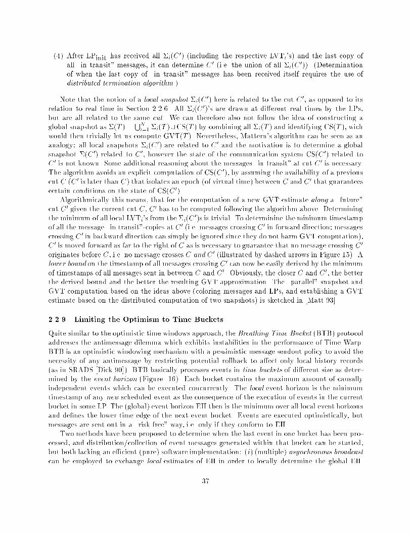
(4) After LPinit has received all �i(C 0) (including the respective LVTi's) and the last copy ofall \in transit" messages, it can determine C0 (i.e. the union of all �i(C0)). (Determinationof when the last copy of \in transit" messages has been received itself requires the use ofdistributed termination algorithm.)Note that the notion of a local snapshot �i(C 0) here is related to the cut C0, as opposed to itsrelation to real time in Section 2.2.6. All �i(C0)'s are drawn at di�erent real times by the LPs,but are all related to the same cut. We can therefore also not follow the idea of constructing aglobal snapshot as �(T ) = SNi=1 �i(T )[CS(T ) by combining all �i(T ) and identifying CS(T ), wichwould then trivially let us compute GVT(T ). Nevertheless, Mattern's algorithm can be seen as ananalogy: all local snapshots �i(C 0) are related to C0 and the motivation is to determine a globalsnapshot �(C 0) related to C 0, however the state of the communication system CS(C 0) related toC0 is not known. Some additional reasoning about the messages \in transit" at cut C0 is necessary.The algorithm avoids an explicit computation of CS(C 0), by assuming the availability of a previouscut C (C 0 is later than C) that isolates an epoch (of virtual time) between C and C 0 that guaranteescertain conditions on the state of CS(C0).Algorithmically this means, that for the computation of a new GVT estimate along a \future"cut C 0 given the current cut C, C 0 has to be computed following the algorithm above. Determiningthe minimum of all local LVTi's from the �i(C 0)s is trivial. To determinine the minimum timestampof all the message \in transit"-copies at C 0 (i.e. messages crossing C0 in forward direction; messagescrossing C0 in backward direction can simply be ignored since they do not harm GVT computation),C0 is moved forward as far to the right of C as is necessary to guarantee that no message crossing C 0originates before C, i.e. no message crosses C and C 0 (illustrated by dashed arrows in Figure 15). Alower bound on the timestamp of all messages crossing C0 can now be easily derived by the minimumof timestamps of all messages sent in between C and C 0. Obviously, the closer C and C0, the betterthe derived bound and the better the resulting GVT approximation. The \parallel" snapshot andGVT computation based on the ideas above (coloring messages and LPs, and establishing a GVTestimate based on the distributed computation of two snapshots) is sketched in [Matt 93].2.2.9 Limiting the Optimism to Time BucketsQuite similar to the optimistic time windows approach, the Breathing Time Bucket (BTB) protocoladdresses the antimessage dilemma which exhibits instabilities in the performance of Time Warp.BTB is an optimistic windowing mechanism with a pessimistic message sendout policy to avoid thenecessity of any antimessage by restricting potential rollback to a�ect only local history records(as in SRADS [Dick 90]). BTB basically processes events in time buckets of di�erent size as deter-mined by the event horizon (Figure 16). Each bucket contains the maximum amount of causallyindependent events which can be executed concurrently. The local event horizon is the minimumtimestamp of any new scheduled event as the consequence of the execution of events in the currentbucket in some LP. The (global) event horizon EH then is the minimum over all local event horizonsand de�nes the lower time edge of the next event bucket. Events are executed optimistically, butmessages are sent out in a \risk free" way, i.e. only if they conform to EH.Two methods have been proposed to determine when the last event in one bucket has been pro-cessed, and distribution/collection of event messages generated within that bucket can be started,but both lacking an e�cient (pure) software implementation: (i) (multiple) asynchronous broadcastcan be employed to exchange local estimates of EH in order to locally determine the global EH.37

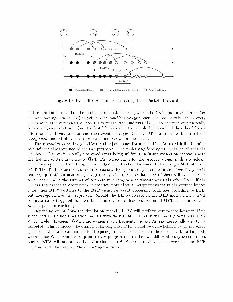
Bucket 1

Committed Event Processed, Uncommitted Event Scheduled Event

Bucket 2

Bucket 3Figure 16: Event Horizons in the Breathing Time Buckets ProtocolThis operation can overlap the bucket computation during which the CS is guaranteed to be freeof event message tra�c. (ii) a system wide nonblocking sync operation can be released by everyLP as soon as it surpasses the local EH estimate, not hindering the LP to continue optimisticallyprogressing computations. Once the last LP has issued the nonblocking sync, all the other LPs areinterrupted and requested to send their event messages. Clearly, BTB can only work e�ciently ifa su�cient amount of events is processed on average in one bucket.The Breathing Time Warp (BTW) [Stei 93] combines features of Time Warp with BTB aimingto eliminate shortcomings of the two protocols. The underlying idea again is the belief that thelikelihood of an optimistically processed event being subject to a future correction decreases withthe distance of its timestamp to GVT. The consequence for the protocol design is thus to releaseevent messages with timestamps close to GVT, but delay the sendout of messages `distant' fromGVT. The BTB protocol operates in twomodes. Every bucket cycle starts in the Time Warp mode,sending up to M outputmessages aggressively with the hope that none of them will eventually berolled back. M is the number of consecutive messages with timestamps right after GVT. If theLP has the chance to optimistically produce more than M outputmessages in the current bucketcycle, then BTW switches to the BTB mode, i.e. event processing continues according to BTB,but message sendout is suppressed. Should the EH be crossed in the BTB mode, then a GVTcomputation is triggered, followed by the invocation of fossil collection. If GVT can be improved,M is adjusted accordingly.Depending on M (and the simulation model), BTW will perform somewhere between TimeWarp and BTB: For simulation models with very small EH BTW will mostly remain in TimeWarp mode. Frequent GVT improvements will frequently adjust M and rarely allow it to beexceeded. This is indeed the desired behavior, since BTB would be overwhelmed by an increasedsynchronization and communication frequency in such a scenario. On the other hand, for large EHwhere Time Warp would overoptimistically progress due to the availability of many events in onebucket, BTW will adapt to a behavior similar to BTB since M will often be exceeded and BTBwill frequently be induced, thus \limiting" optimism.38

Step LP1 LP1IB LVT S EVL OB IB LVT S EVL OB0 | 0.00 2 T1@0.17;T1@0.37 | | 0.00 1 T2@0.51 |1 | 0.17 1 T1@0.37 h 1; P2; 0.17 i | 0.51 0 | h 1; P1; 0.51 i2 h 1; P1; 0.51 i 0.37 1 T1@0.73 h 1; P2; 0.37 i h 1; P2; 0.17 i 0.56 0 | h 1; P1; 0.56 i3 h 1; P1; 0.56 i 0.73 1 T1@0.90 h 1; P2; 0.73 i h 1; P2; 0.37 i 0.56 1 T2@0.79 |4 | 0.90 0 | h 1; P2; 0.90 i h 1; P2; 0.73 i 0.78 1 T2@0.79 h 1; P1; 0.78 iTable 4: Motivation for Probabilistic LP Simulation2.2.10 Probabilistic OptimismA communication interface CI that considers the CMB protocol and Time Warp as two extremesin a spectrum of possibilities to synchronize LP's LVT advancements is the probabilistic distributedDES protocol [Fers 94c]. Let the occurrence of an event e, t(e) = LVTi, in some LPi be causal(!) for a future event e0 with t(e0) = LVTi + �(t) in LPj with probability P [e ! e0], i.e. event ewith some probability changes state variables in Sj with incluence on e0. Then the CMB \blockuntil safe-to-process"-rule appears adequate for P [e ! e0] = 1, and is overly pessimistic for casesP [e ! e0] < 1 since awaiting the decision whether (e ! e0) or (e 6! e0) hinders the (probablycorrect) concurrent execution of events e and e0 in di�erent LPs. Clearly, if P [e ! e0] � 1 anoptimistic strategy could have executed e0 concurrently to e most of the time. This argumentmainly motivates the use of an optimistic CI for simulation models with nondeterministic eventcausalities. On the other hand, as already seen with the discussion of rollback chains, an optimisticLP might tend towards overoptimism, i.e. optimism lacking rational justi�cation. The probabilisticprotocol aims to exploit information on the dynamic simulation behavior in order to be able toallow in every simulation step just that amount of optimism that can be justi�ed.To give an intuition on the justi�cation of optimism look again at the parallel simulation of thesmall simulation model in Figure 7 together with the future list, and the parallel execution of lazycancellation Time Warp in Figure 3. At the beginning of step 3 LP2 at LVT = 0:56 (= LVT atthe end of step 2) faces the straggler h 1; P2; 0.37 i in its IQ; the next element in LP2's future listis 0.42. Since the e�ect of the straggler is in the local future of LP2, i.e. h T2@(0.37+0.42) i, thelazy rollback strategy applies and rollback is avoided at all. The event h T2@0.79 i is executed inthat step, setting LVT = 0.79, and the outputmessage h 1; P1; 0.79 i is generated (OQ) and sentat the end of the step. Unfortunately, in step 4 a new straggler h 1; P2; 0.73 i is observed in IQof LP2, but now with the e�ect that at time t = 0:73 + 0:05 < LVT = 0:79 LP2 is forced to rollback (Figure 3). Indeed, LP2 in step 3 generated and sent out h 1; P1; 0.79 i without consideringany information whether the implicit optimism is justi�ed or not. If LP2 would have observed thatit received \on the average" one input message per step, with an \average" timestamp incrementof 0.185, it might have established a hypothesis that in step 4 a message is expected to arrivewith an estimated timestamp of 0.37+0.185 = 0.555 (= timestamp of previous message + averageincrement). Taking this as an alarm for potential rollback, LP2 could have avoided the propagationof the local optimistic simulation progression by e.g. delaying the sendout of h 1; P1; 0.79 i forone step. This is illustrated in Figure 4: LP2 just takes the input message from IQ and schedulesthe event h T2@0.79 i in EVL, but does not process it. Instead, the execution is delayed until thehypothesis upon the next message's timestamp is veri�ed. The next message is h 1; P1; 0.73 i, thehypothesis can be dropped, and a new event h T2@0.78 i is scheduled and processed next. Actuallytwo rollbacks and the corresponding sending of antimessages could be avoided by applying theprobabilistic simulation scheme. 39

t̂ = ee i + ∆̂ (δ1 ... δn )

s t

0

1

α (t-s)

α

CDF

internal event

external event

simulated time

virtual time (VT)

δ1 ee i+1ee iδn

[ ]s t0

... ......

t-s2

∆̂ =Figure 17: Motivation for the Probabilistic DDESAs a more general argument, assume the timestamp of the next messagem carrying the externalevent eei+1 to arrive at LPj to be in the time interval [s; t] (t can be arbitrarily large), andthat LVTj has advanced to a certain value (see Figure 17). External events have been receivedin the past and respected chronologically, some of the internal events are already scheduled forLPj 's future. Let the probability of the actual timestamp t(eei+1) of the forthcoming message beP [t� = x] = 1t�s 8x 2 [s; t], i.e. the next external event occurrence is equally likely for all points in[s; t]. The CMB protocol could have safely simulated all the internal events t(iek) < t(eei+1), butwill block at LVT = s. Under the assumptions made above, however, by blocking, CMB fails touse a (1��) chance to produce useful simulation work by progressing over s and executing internalevents in the time interval [s; s+ �(t� s)]. Again an overpessimism is identi�ed for CMB, at leastfor small values of �. Time Warp on the other hand would proceed simulating internal events evenafter surpassing t. This is overly optimistic in the sense that every internal event with t(iek) > twill de�nitely (with probability of 1) have to be invalidated.The probabilistic protocol appears to be a performance e�cient compromise between the twoclassical approaches. As opposed to CMB, it allows trespassing of s and progressing simulationup until bt = eei + b�(�1; �2; : : : �n), s � bt � t, where bt(�) is an estimate based on the di�erences�k = t(eei�k+1) � t(eei�k) of the observed arrival instants A = (t(eei�n+1); t(eei�n+2); : : : t(eei)),n being the size of the (history) observation window. Compared to Time Warp it prevents fromoveroptimistically di�using incorrect simulations too far ahead into the simulated future, and thusavoids unnecessary communication overhead due to rollbacks and consequential rollback chains.The message arrival patterns observed are used to adapt the LP to a synchronization behaviorthat is the best tradeo� among blocking and optimistically progressing with respect to the paral-lelism inherent to the simulation model, by conditioning the execution of S3.2 through S3.11 inthe algorithm in Figure 11 to a probabilistic \throttle". Assume that Ai = (t(eek�n+1); t(eek�n+2),: : : t(eek)) is maintained in LPj for every (input) channel chi;j , and that for chi;j bti is estimatedwith some con�dence 0 � �(bti) � 1. The probabilistic protocol is then obtained by replacing S3.2{ S3.11 in Figure 11 with: 40

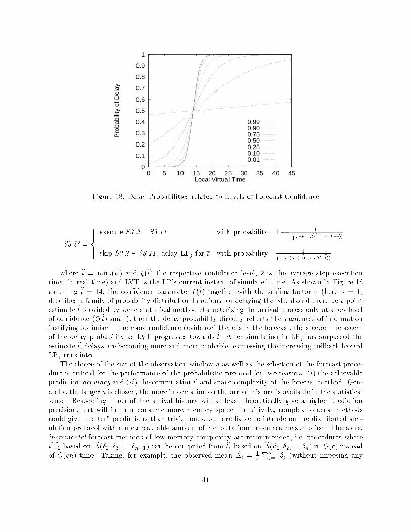
0

0.1

0.2

0.3

0.4

0.5

0.6

0.7

0.8

0.9

1

0 5 10 15 20 25 30 35 40 45

Pro

babi

lity

of D

elay

Local Virtual Time

0.990.900.750.500.250.100.01Figure 18: Delay Probabilities related to Levels of Forecast Con�denceS3.2' = 8>><>>: execute S3.2 { S3.11 with probability 1� 11+e�( �(bt) (LV T�bt))skip S3.2 { S3.11 , delay LPj for s with probability 11+e�( �(bt) (LV T�bt))where bt = mini(bti) and �(bt) the respective con�dence level, s is the average step executiontime (in real time) and LVT is the LP's current instant of simulated time. As shown in Figure 18assuming bt = 14, the con�dence parameter �(bt) together with the scaling factor (here = 1)describes a family of probability distribution functions for delaying the SE: should there be a pointestimate bt provided by some statistical method characterizing the arrival process only at a low levelof con�dence (�(bt) small), then the delay probability directly re ects the vagueness of informationjustifying optimism. The more con�dence (evidence) there is in the forecast, the steeper the ascentof the delay probability as LVT progresses towards bt. After simulation in LPj has surpassed theestimate bt, delays are becoming more and more probable, expressing the increasing rollback hazardLPj runs into.The choice of the size of the observation window n as well as the selection of the forecast proce-dure is critical for the performance of the probabilistic protocol for two reasons: (i) the achievableprediction accuracy and (ii) the computational and space complexity of the forecast method. Gen-erally, the larger n is chosen, the more information on the arrival history is available in the statisticalsense. Respecting much of the arrival history will at least theoretically give a higher predictionprecision, but will in turn consume more memory space. Intuitively, complex forecast methodscould give \better" predictions than trivial ones, but are liable to intrude on the distributed sim-ulation protocol with a nonacceptable amount of computational resource consumption. Therefore,incremental forecast methods of low memory complexity are recommended, i.e. procedures wheredti+1 based on b�(�2; �3; : : : �n+1) can be computed from bti based on b�(�1; �2; : : : �n) in O(c) insteadof O(cn) time. Taking, for example, the observed mean b�i = 1nPnj=1 �j (without imposing any41

observation window) as the basis for an estimate of bt, then upon the availability of the next �n+1,dti+1 could be computed based on b�n+1 = n b�n + �n+1n + 1 :A possibility to weight recent history more heavily than past history could be an exponentialsmoothing of the observation vector by a smoothing factor � (j1� �j < 1):b�n+1 = nXi=1 �(1� �)i�1�n+1�i:b� in this case has the incremental formb�n+1 = ��n+1 + (1� �) b�nThe arrival process of messages via a channel could also be considered to originate from an un-derlying but unknown stochastic process. Autoregressive moving average (ARMA) process models[Broc 91] are a reasonable method to characterize that process by the relationship among a seriesof empirical non-independent observations fXig = (X1; X2; : : :Xn) (in our case = (�1; �2; : : :�n)).Assuming fXig is already a centered series (i.e. transformed with respect to the series mean �,Xi = �i � �), then Xt = �1Xt�1 + �2Xt�2 + : : : + �pXt�p + �t is a pure autoregressive processof order p (AR[p]) with �t being a sequence of (independent, identically distributed) white noiserandom disturbances. Xt is usually called the centered response, and �i are parameters that canbe be estimated from the realizations in various di�erent ways [Broc 91], e.g. maximum likelihoodor the (recursive) Yule-Walker method. Xt = �t + �1�t�1 + �2�t�2 + : : :+ �q�t�q is a pure movingaverage process of order q (MA[q]) with E(�i) = 0, Var(�i) = �2� and E(Xt) = 0. A (mixed) processARMA[p; q] is now de�ned as Xt = pXi=1 �iXt�i + �t + qXi=1 �i�t�iStationary ARMA[p; q] processes are able to explain short term trends and even cycles in theobservation pattern, thus characterizing the transient behavior of message arrivals (in the case thesimulation induces phases of message arrival patterns) to some extent. Several methods are avail-able for ARMA[p; q] processes to forecast Xt+1 from fXig. An incremental way, for example, is theDurbin-Levinson method for one-step best linear predictions. Non-stationary series Xt+1 can betreated with ARIMA[p; d; q] processes, d in this case denoting the di�erencing order, i.e. the num-ber of di�erencing transformations required to induce stationarity for the non-stationary ARIMAprocess (ARIMA[p; 0; q]� ARMA[p; q]). Besides the basic statistical methods described above, also(nonlinear) mechanisms developed in control theory, machine learning and neural network simu-lations as well as hidden markov models could be used to control optimism in the probabilisticprotocol.The major strength of the probabilistic protocol is that the optimism of Time Warp can beautomatically controlled by the model parallelism available as expressed by the likelihood of futuremessages, and can even adapt to a transient behavior of the simulated model. The asymptoticbehavior of the protocol for simulation models with P [e ! e0] ' 1 (for all pairs (e; e0)) is close toCMB, while for models with P [e! e0] ' 0 it is arbitrarily close to (a throtteled) Time Warp.42

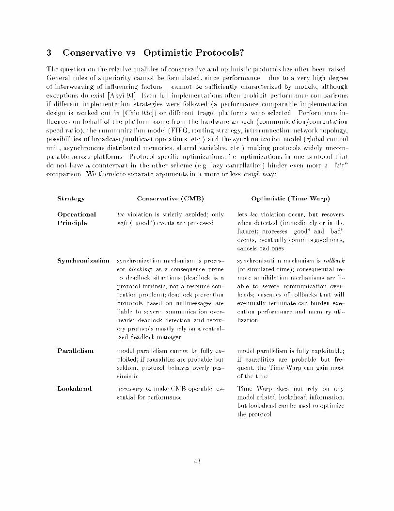
3 Conservative vs. Optimistic Protocols?The question on the relative qualities of conservative and optimistic protocols has often been raised.General rules of superiority cannot be formulated, since performance { due to a very high degreeof interweaving of in uencing factors { cannot be su�ciently characterized by models, althoughexceptions do exist [Akyi 93]. Even full implementations often prohibit performance comparisonsif di�erent implementation strategies were followed (a performance comparable implementationdesign is worked out in [Chio 93c]) or di�erent traget platforms were selected. Performance in- uences on behalf of the platform come from the hardware as such (communication/computationspeed ratio), the communication model (FIFO, routing strategy, interconnection network topology,possibilities of broadcast/multicast operations, etc.) and the synchronization model (global controlunit, asynchronous distributed memories, shared variables, etc.) making protocols widely uncom-parable across platforms. Protocol speci�c optimizations, i.e. optimizations in one protocol thatdo not have a counterpart in the other scheme (e.g. lazy cancellation) hinder even more a \fair"comparison. We therefore separate arguments in a more or less rough way:Strategy Conservative (CMB) Optimistic (Time Warp)OperationalPrinciple lcc violation is strictly avoided; onlysafe (\good") events are processed lets lcc violation occur, but recoverswhen detected (immediately or in thefuture); processes \good" and \bad"events, eventually commits good ones,cancels bad onesSynchronization synchronization mechanism is proces-sor blocking; as a consequence proneto deadlock situations (deadlock is aprotocol intrinsic, not a resource con-tention problem); deadlock preventionprotocols based on nullmessages areliable to severe communication over-heads; deadlock detection and recov-ery protocols mostly rely on a central-ized deadlock manager synchronization mechanism is rollback(of simulated time); consequential re-mote annihilation mechanisms are li-able to severe communication over-heads; cascades of rollbacks that willeventually terminate can burden exe-cution performance and memory uti-lizationParallelism model parallelism cannot be fully ex-ploited; if causalities are probable butseldom, protocol behaves overly pes-simistic model parallelism is fully exploitable;if causalities are probable but fre-quent, the Time Warp can gain mostof the timeLookahead necessary to make CMB operable, es-sential for performance Time Warp does not rely on anymodel related lookahead information,but lookahead can be used to optimizethe protocol43

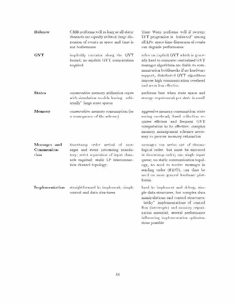
Balance CMB performs well as long as all staticchannels are equally utilized; large dis-persion of events in space and time isnot bothersome Time Warp performs well if averageLVT progression is \balanced" amongall LPs; space time dispersion of eventscan degrade performanceGVT implicitly executes along the GVTbound; no explicit GVT computationrequired relies on explicit GVT which is gener-ally hard to compute; centralized GVTmanager algorithms are liable to com-munication bottlenecks if no hardwaresupport; distributed GVT algorithmsimpose high communication overheadand seem less e�ectiveStates conservative memory utilization copeswith simulation models having \arbi-trarily" large state spaces performs best when state space andstorage requirement per state is smallMemory conservative memory consumption (asa consequence of the scheme) aggressive memory consumption; statesaving overhead; fossil collection re-quires e�cient and frequent GVTcomputation to be e�ective; complexmemory management schemes neces-sary to prevent memory exhaustionMessages andCommunica-tion timestamp order arrival of mes-sages and event processing manda-tory; strict separation of input chan-nels required; static LP interconnec-tion channel topology; messages can arrive out of chrono-logical order, but must be executedin timestamp order; one single inputqueue; no static communication topol-ogy; no need to receive messages insending order (FIFO), can thus beused on more general hardware plat-formsImplementation straightforward to implement; simplecontrol and data structures hard to implement and debug; sim-ple data structures, but complex datamanipulations and control structures;\tricky" implementations of control ow (interrupts) and memory organi-zation essential; several performancein uencing implementation optimiza-tions possible44

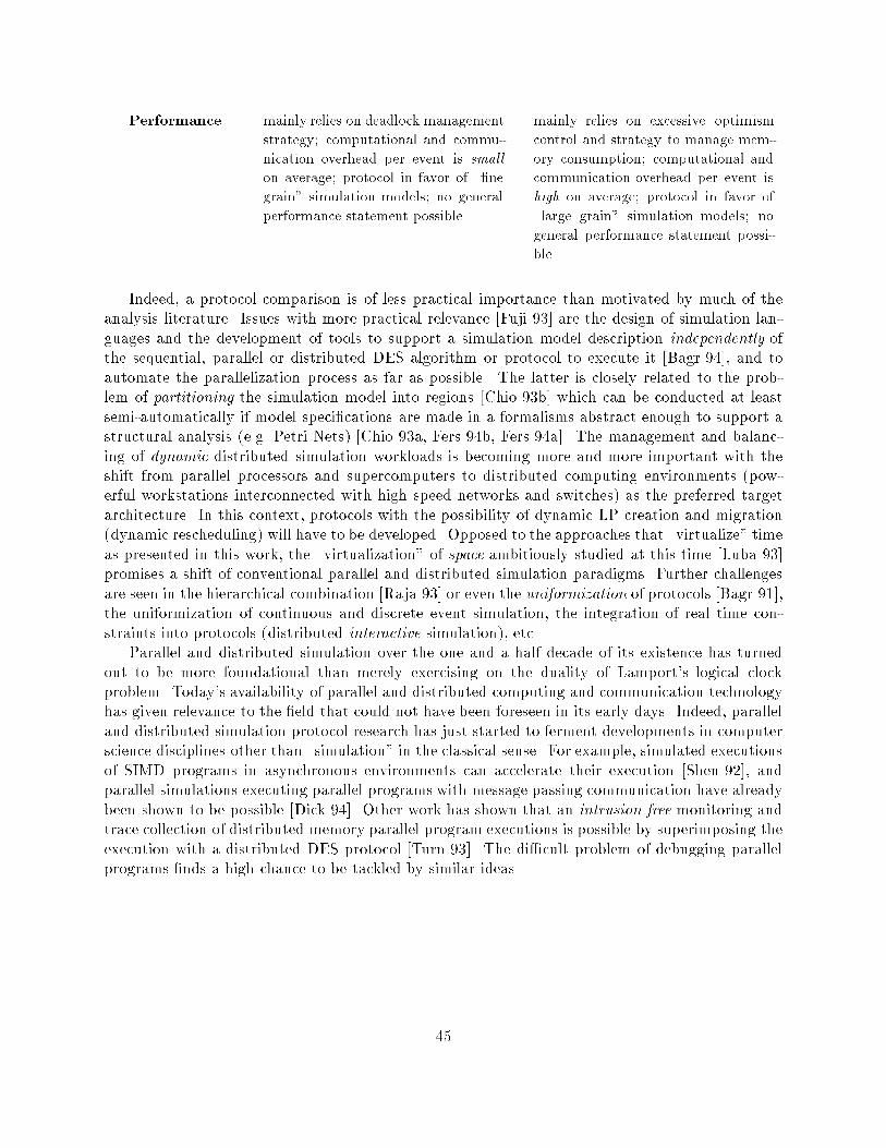
Performance mainly relies on deadlock managementstrategy; computational and commu-nication overhead per event is smallon average; protocol in favor of \�negrain" simulation models; no generalperformance statement possible mainly relies on excessive optimismcontrol and strategy to manage mem-ory consumption; computational andcommunication overhead per event ishigh on average; protocol in favor of\large grain" simulation models; nogeneral performance statement possi-bleIndeed, a protocol comparison is of less practical importance than motivated by much of theanalysis literature. Issues with more practical relevance [Fuji 93] are the design of simulation lan-guages and the development of tools to support a simulation model description independently ofthe sequential, parallel or distributed DES algorithm or protocol to execute it [Bagr 94], and toautomate the parallelization process as far as possible. The latter is closely related to the prob-lem of partitioning the simulation model into regions [Chio 93b] which can be conducted at leastsemi-automatically if model speci�cations are made in a formalisms abstract enough to support astructural analysis (e.g. Petri Nets) [Chio 93a, Fers 94b, Fers 94a]. The management and balanc-ing of dynamic distributed simulation workloads is becoming more and more important with theshift from parallel processors and supercomputers to distributed computing environments (pow-erful workstations interconnected with high speed networks and switches) as the preferred targetarchitecture. In this context, protocols with the possibility of dynamic LP creation and migration(dynamic rescheduling) will have to be developed. Opposed to the approaches that \virtualize" timeas presented in this work, the \virtualization" of space ambitiously studied at this time [Luba 93]promises a shift of conventional parallel and distributed simulation paradigms. Further challengesare seen in the hierarchical combination [Raja 93] or even the uniformization of protocols [Bagr 91],the uniformization of continuous and discrete event simulation, the integration of real time con-straints into protocols (distributed interactive simulation), etc.Parallel and distributed simulation over the one and a half decade of its existence has turnedout to be more foundational than merely exercising on the duality of Lamport's logical clockproblem. Today's availability of parallel and distributed computing and communication technologyhas given relevance to the �eld that could not have been foreseen in its early days. Indeed, paralleland distributed simulation protocol research has just started to ferment developments in computerscience disciplines other than \simulation" in the classical sense. For example, simulated executionsof SIMD programs in asynchronous environments can accelerate their execution [Shen 92], andparallel simulations executing parallel programs with message passing communication have alreadybeen shown to be possible [Dick 94]. Other work has shown that an intrusion free monitoring andtrace collection of distributed memory parallel program executions is possible by superimposing theexecution with a distributed DES protocol [Turn 93]. The di�cult problem of debugging parallelprograms �nds a high chance to be tackled by similar ideas.45

4 Sources of Literature and Further ReadingComprehensive overviews on the �eld of parallel and distributed simulation are the surveys byRichter and Walrand [Rich 89], Fujimoto [Fuji 90], and most recently Nicol and Fujimoto [Nico 94].The primary reading for Time Warp is [Je� 85a], for conservative protocols it is [Misr 86]. Themost relevant literature appears in the frame of the� Workshop on Parallel and Distributed Simulation (PADS),formerly (while being held as part of the SCS Multiconference) published as the Proceedings ofthe SCS Multiconference on Distributed Simulation. PADS's primary focus is on the developmentand analysis of new protocols, recently also on viability studies, successful applications, tools anddevelopment environments. Conferences and workshops that have published application, analysis,performance, implementation and comparison related studies are� the annual Winter Simulation Conference (WSC),� the ACM Sigmetrics Conference on Measurement & Modeling of Computer Systems.� the Annual Simulation Symposium, and� a variety of conferences and workshops related to parallel and distributed processing.Outstanding contributions can be found in the following periodicals:� ACM Trans. on Modeling and Computer Simulation (TOMACS)� IEEE Trans. on Parallel and Distributed Systems� Journal of Parallel and Distributed Computing� IEEE Trans. on Software Engineering, IEEE Trans. on Computers� International Journal in Computer Simulation46

References[Akyi 93] I. F. Akyildiz, L. Chen, R. Das, R. M. Fujimoto, and R. F. Serfozo. \The E�ect ofMemory Capacity on Time Warp Performance". Journal of Parallel and DistributedComputing, Vol. 18, No. 4, pp. 411{422, August 1993.[Bagr 91] R. Bagrodia, K. M. Chandy, and W. T. Liao. \A Unifying Framework for DistributedSimulation". ACM Transactions on Modeling and Computer Simulation, Vol. 1, No. 4,pp. 348{385, October 1991.[Bagr 94] R. L. Bagrodia, V. Jha, and J. Waldorf. \The Maisie Environment for Parallel Simula-tion". In: Proc. of the 27th Annual Simulation Symposium, La Jolla, California, April11-15, 1994, pp. 4 { 12, IEEE Computer Society Press, Los Alamitos, California, 1994.[Baik 85] D. Baik and B. P. Zeigler. \Perfromance Evaluation of Hierarchical Distributed Sim-ulators". In: Proc. of the 1985 Winter Simulation Conference, pp. 421 { 427, SCS,1985.[Bain 88] W. L. Bain and D. S. Scott. \An algorithm for time synchronization in distributeddiscrete event simulation". In: B. Unger and D. Je�erson, Eds., Proceedings of the SCSMulticonference on Distributed Simulation, 19 (3), pp. 30{33, SCS, February 1988.[Ball 90] D. Ball and S. Hoyt. \The Adaptive Time-Warp Concurrency Control Algorithm".In: D. Nicol, Ed., Distributed Simulation. Proceedings of the SCS Multiconference onDistributed Simulation, pp. 174 { 177, Society for Computer Simulation, San Diego,California, 1990. Simulation Series, Volume 22, Number 1.[Bell 90] S. Bellenot. \Global virtual time algorithms". In: Proceedings of the Multiconferenceon Distributed Simulation., pp. 122 { 127, 1990.[Broc 91] P. J. Brockwell and R. A. Davis. Time Series: Theory and Methods. Springer Verlag,New York, 1991.[Brya 84] R. E. Bryant. \A Switch-Level Model and Simulator for MOS Digital Systems". IEEETransactions on Computers, Vol. C-33, No. 2, pp. 160{177, February 1984.[Cai 90] W. Cai and S. J. Turner. \An Algorithm for Distributed Discrete-Event Simulation -The `Carrier Null Message' Approach". In: Proceedings of the SCS Multiconference onDistributed Simulation Vol. 22 (1), pp. 3{8, SCS, January 1990.[Chan 79] K. M. Chandy and J. Misra. \Distributed Simulation: A Case Study in Design andVer��cation of Distributed Programs". IEEE Transactions on Software Engineering,Vol. SE-5, No. 5, pp. 440{452, Sep. 1979.[Chan 81] K. M. Chandy and J. Misra. \Asynchronous Distributed Simulation via a Sequenceof Parallel Computations". Communications ACM, Vol. 24, No. 11, pp. 198{206, Nov.1981.[Chan 83] K. M. Chandy, J. Misra, and L. M. Haas. \Distributed Deadlock Detection". ACMTransactions On Computer Systems, Vol. 1, No. 2, pp. 144{156, May 1983.47

[Chan 85] K. M. Chandy and J. Lamport. \Distributed Snapshots: Determining Global Statesof Distributed Systems.". ACM Transactions on Computer Systems, Vol. 3, No. 1,pp. 63{75, 1985.[Chio 93a] G. Chiola and A. Ferscha. \Distributed Simulation of Petri Nets". IEEE Parallel andDistributed Technology, Vol. 1, No. 3, pp. 33 { 50, Aug. 1993.[Chio 93b] G. Chiola and A. Ferscha. \Distributed Simulation of Timed Petri Nets: Exploitingthe Net Structure to Obtain E�ciency". In: M. Ajmone Marsan, Ed., Proc. of the 14thInt. Conf. on Application and Theory of Petri Nets 1993, Chicago, June 1993, pp. 146{ 165, Springer Verlag, Berlin, 1993.[Chio 93c] G. Chiola and A. Ferscha. \Performance Comparable Implementation Design of Syn-chronization Protcols for Distributed Simulation". Tech. Rep. ACPC-TR 93-20, Aus-trian Center for Parallel Computation, 1993.[Conc 85] A. I. Concepcion. \Mapping Distributed Simulators onto the Hierarchical MultibusMultiprocessor Architecture". In: P. Reynolds, Ed., Proc. of the SCS Multiconferenceon Distributed Simulation, pp. 8{13, Society for Computer Simulation, 1985.[Das 94] S. R. Das and R. M. Fujimoto. \An Adaptive Memory Management Protocol forTime Warp Parallel Simulation". In: Proc. of the 1994 ACM Sigmetrics Conference onMeasurement and Modeling of Computer Systems, Nashville, 1994, pp. 201{210, ACM,1994.[Dick 90] P. M. Dickens and P. F. Reynolds. \SRADS with Local Rollback". In: Proceedingsof the SCS Multiconference on Distributed Simulation Vol. 22 (1), pp. 161{164, SCS,January 1990.[Dick 94] P. M. Dickens, P. Heidelberger, and D. M. Nicol. \Parallelized Direct Execution Sim-ulation of Message-Passing Parallel Programs". Tech. Rep., ICASE, NASA LangleyResearch Center, Hampton, VA, 1994. submitted for publication.[DSou 94] L. M. D'Souza, X. Fan, and P. A. Wilsey. \pGVT: An Algorithm for Accurate GVT Es-timation". In: , Ed., Proc. of the 8th Workshop on Parallel and Distributed Simulation,p. , IEEE Computer Society Press, 1994. to appear.[Feld 90] R. E. Felderman and L. Kleinrock. \An Upper Bound on the Improvement of Asyn-chronous versus Synchronous Distributed Processing". In: D. Nicol, Ed., Proc. of theSCS Multiconf. on Dist. Sim., pp. 131 { 136, Jan 1990.[Fers 94a] A. Ferscha. \Concurrent Execution of Time Petri Nets". In: J. D. Tew and S. Mani-vannan, Eds., Proceedings of the 1994 Winter Simulation Conference, 1994.[Fers 94b] A. Ferscha and G. Chiola. \Accelerating the Evaluation of Parallel Program Perfor-mance Models using Distributed Simulation". In: Proc. of. the 7th Int. Conf. on Mod-elling Techniques and Tools for Computer Performance Evaluation., 1994.48

[Fers 94c] A. Ferscha and G. Chiola. \Self-Adaptive Logical Processes: the Probabilistic Dis-tributed Simulation Protocol". In: Proc. of the 27th Annual Simulation Symposium,LaJolla, 1994, IEEE Computer Society Press, 1994.[Fuji 90] R. M. Fujimoto. \Parallel Discrete Event Simulation". Communications of the ACM,Vol. 33, No. 10, pp. 30{53, October 1990.[Fuji 93] R. M. Fujimoto. \Parallel Discrete Event Simulation: Will the Field Survive?". ORSAJournal of Computing, Vol. 5, No. 3, pp. 218{230, 1993.[Gafn 88a] A. Gafni. \Rollback Mechanisms for Optimistic Distributed Simulation Systems". In:Proc. of the SCS Multiconference on Distributed Simulation 19, pp. 61{67, 1988.[Gafn 88b] A. Gafni. \Rollback Mechanisms for Optimistic Distributed Simulation Systems". In:B. Unger and D. Je�erson, Eds., Proceedings of the SCS Multiconference on DistributedSimulation, 19 (3), pp. 61{67, SCS, February 1988.[Gros 88] B. Groselj and C. Tropper. \The time-of-next-event algorithm". In: B. Unger andD. Je�erson, Eds., Proceedings of the SCS Multiconference on Distributed Simulation,19 (3), pp. 25{29, SCS, February 1988.[Je� 85a] D. A. Je�erson. \Virtual Time". ACM Transactions on Programming Languages andSystems, Vol. 7, No. 3, pp. 404{425, July 1985.[Je� 85b] D. Je�erson and H. Sowizral. \Fast Concurrent Simulation Using the Time WarpMechanism". In: P. Reynolds, Ed., Distributed Simulation 1985, pp. 63{69, SCS-TheSociety for Computer Simulation, Simulation Councils, Inc., La Jolla, California, 1985.[Je� 90] D. Je�erson. \Virtual Time II: the cancelback protocol for storage management inTime Warp". In: Proc. of the 9th Annual ACM Symposium on Principles of DistributedComputing, pp. 75{90, ACM, New York, 1990.[Je� 91] D. Je�erson and P. Reiher. \Supercritical Speedup". In: A. H. Rutan, Ed., Proceedingsof the 24th Annual Simulation Symposium, New Orleans, Louisiana, USA, April 1-5,1991., pp. 159{168, IEEE Computer Society Press, 1991.[Lamp 78] L. Lamport. \Time, clocks, and the ordering of events in distributed systems". Com-munications of the ACM, Vol. 21, No. 7, pp. 558 { 565, Jul 1978.[Lin 90] Y.-B. Lin and E. Lazowska. \Determining the Global Virtual Time in a DistributedSimulation". In: 1990 International Conference on Parallel Processing, pp. III{201{III{209, 1990.[Lin 91] Y.-B. Lin and B. R. Preiss. \Optimal Memory Management for Time Warp ParallelSimulation". ACM Transactions on Modeling and Computer Simulation, Vol. 1, No. 4,pp. 283{307, October 1991.[Lin 93] Y.-B. Lin, B. Preiss, W. Loucks, and E. Lazowska. \Selecting the Checkpoint Intervalin Time Warp Simulation". In: R. Bagrodia and D. Je�erson, Eds., Proc. of the 7thWorkshop on Parallel and Distributed Simulation, pp. 3{10, IEEE Computer SocietyPress, Los Alamitos, CA, 1993. 49

[Luba 88] B. D. Lubachevsky. \Bounded lag distributed discrete event simulation". In: B. Ungerand D. Je�erson, Eds., Proceedings of the SCS Multiconference on Distributed Simula-tion, 19 (3), pp. 183{191, SCS, February 1988.[Luba 91] B. Lubachevsky, A. Weiss, and A. Shwartz. \An Analysis of Rollback-Based Sim-ulation". ACM Transactions on Modeling and Computer Simulation, Vol. 1, No. 2,pp. 154{193, April 1991.[Luba 93] B. D. Lubachevsky. \Relaxation for Massively Parallel Discrete Event Simulation". In:L. Donatiello and R. Nelson, Eds., Performance Evaluation of Computer and Commu-nication Systems, pp. 307 { 329, Springer Verlag, 1993.[Matt 87] F. Mattern. \Algorithms for distributed termination detection". Distributed Computing,Vol. 2, pp. 161{175, 1987.[Matt 93] F. Mattern. \E�cient Algorithms for Distributed Snapshots and Global Virtual TimeApproximation". Journal of Parallel and Distributed Computing, Vol. 18, No. 4,pp. 423{434, August 1993.[Misr 86] J. Misra. \Distributed Discrete-Event Simulation". ACM Computing Surveys, Vol. 18,No. 1, pp. 39{65, March 1986.[Nico 88] D. M. Nicol. \Parallel Discrete-Event Simulation OF FCFS Stochastic Queueing Net-works". In: Proceedings of the ACM/SIGPLAN PPEALS 1988, pp. 124 { 137, 1988.[Nico 91] D. M. Nicol. \Performance bounds on parallel self-initiating discrete event simulations".ACM Transactions on Modeling and Computer Simulation, Vol. 1, No. 1, pp. 24 { 50,Jan 1991.[Nico 94] D. Nicol and R. Fujimoto. \Parallel Simulation Today". to appear in: OperationsResearch, 1994.[Peac 79] J. K. Peacock, J. W. Wong, and E. G. Manning. \Distributed Simulation using aNetwork of Processors.". Computer Networks, Vol. 3, No. 1, pp. 44{56, 1979.[Prak 91] A. Prakash and R. Subramanian. \Filter: An Algorithm for Reducing Cascaded Roll-backs in Optimistic Distributed Simulation". In: A. H. Rutan, Ed., Proceedings of the24th Annual Simulation Symposium, New Orleans, Louisiana, USA, April 1-5, 1991.,pp. 123{132, IEEE Computer Society Press, 1991.[Raja 93] H. Rajaei, R. Ayani, and L. E. Thorelli. \The Local Time Warp Approach to ParallelSimulation". In: R. Bagrodia and D. Je�erson, Eds., Proc. of the 7th Workshop onParallel and Distributed Simulation, pp. 119{126, IEEE Computer Society Press, LosAlamitos, CA, 1993.[Reih 90] P. L. Reiher, R. M. Fujimoto, S. Bellenot, and D. Je�erson. \Cancellation Strategiesin Optimistic Execution Systems". In: Proceedings of the SCS Multiconference onDistributed Simulation Vol. 22 (1), pp. 112{121, SCS, January 1990.50

[Rich 89] R. Richter and J. C. Walrand. \Distributed Simulation of Discrete Event Systems".Proceedings of the IEEE, Vol. 77, No. 1, pp. 99 { 113, Jan 1989.[Sama 85] B. Samadi. Distributed Simulation algorithms and performance analysis. PhD thesis,University of California, Los Angeles, 1985.[Shen 92] S. Shen and L. Kleinrock. \The Virtual-Time Data-Parallel Machine". In: Proc. of the4th Symposium on the Frontiers of Massively Parallel Computation, pp. 46{53, IEEECompute Society Press, 1992.[Soko 88] L. M. Sokol, D. P. Briscoe, and A. P. Wieland. \MTW: a strategy for schedulingdiscrete simulation events for concurrent execution.". In: Proc. of the SCS Multiconf.on Distributed Simulation, pp. 34 { 42, 1988.[Stei 93] J. S. Steinmann. \Breathing Time Warp". In: R. Bagrodia and D. Je�erson, Eds.,Proc. of the 7th Workshop on Parallel and Distributed Simulation, pp. 109{118, IEEEComputer Society Press, Los Alamitos, CA, 1993.[Turn 93] S. J. Turner and W. Cai. \The \Logical Clocks" Approach to the Visualization ofParallel Programs". In: G. Haring and G. Kotsis, Eds., Performance Measurement andVisualization of Parallel Systems, pp. 45{66, North Holland, 1993.[Venk 86] K. Venkatesh, T. Radhakrishnan, and H. F. Li. \Discrete Event Simulation in a Dis-tributed System". In: IEEE COMPSAC, pp. 123 { 129, IEEE Computer Society Press,1986.

51