Embed Size (px)
Citation preview

Paraglacial sediment storage quantification in the
Turtmann Valley, Swiss Alps
Dissertation
zur
Erlangung des Doktorgrades (Dr. rer. nat.)
der
Mathematisch-Naturwissenschaftlichen Fakultät
der
Rheinischen Friedrich-Wilhelms-Universität Bonn
vorgelegt von
Jan-Christoph Otto
aus
Lemgo
Bonn 2006

Angefertigt mit Genehmigung der Mathematisch-Naturwissenschaftlichen
Fakultät der Rheinischen Friedrich-Wilhelms-Universität Bonn
1. Referent: Prof. Dr. Richard Dikau
2. Referent: Prof. Dr. Lothar Schrott
Tag der Promotion: 20.11.06
Diese Dissertation ist auf dem Hochschulschriftenserver der ULB Bonn http://hss.ulb.uni-bonn.de/diss_online elektronisch publiziert.

I
CONTENTS
CONTENTS I
LIST OF FIGURES III
LIST OF TABLES VII
1 PROBLEM STATEMENT AND MAIN OBJECTIVES 1
2 SCIENTIFIC FRAMEWORK 3
2.1 MOUNTAIN ENVIRONMENTS AS GEOMORPHOLOGICAL SYSTEMS 3
2.1.1 Time and space in mountain geosystems 8
2.2 THE SEDIMENT BUDGET APPROACH 11
2.2.1 Denudation rates and sediment yield 16
2.2.2 Sediment budget and storage quantification 17
2.3 EVOLUTION OF MOUNTAIN LANDSCAPE SYSTEMS 21
2.3.1 Uplift and erosion of mountains 21
2.3.2 The paraglacial sedimentation cycle 23
2.4 SEDIMENT STORAGE LANDFORMS 30
2.4.1 Talus slopes and talus cones 30
2.4.2 Block slopes 33
2.4.3 Rockglaciers 34
2.4.4 Moraines 36
2.4.5 Rock fall deposits 37
2.4.6 Alluvial deposits 38
3 METHODS FOR SEDIMENT STORAGE ANALYSIS 40
3.1 GEOMORPHOLOGICAL SYSTEM AND LAND SURFACE PATTERN ANALYSIS 40
3.2 LANDFORM CLASSIFICATION 42
3.2.1 Derivation of primary attributes 42
3.2.2 Derivation of secondary attributes 43
3.3 TOPOGRAPHICAL, DIGITAL IMAGERY AND GEOMORPHOLOGICAL BASE DATA 45
3.4 METHODS FOR SEDIMENT STORAGE QUANTIFICATION 46
3.4.1 Shallow subsurface geophysical investigations 46 3.4.1.1 Seismic refraction (SR) 47 3.4.1.2 2D- electrical resistivity tomography (ERT) 52 3.4.1.3 Ground penetrating radar (GPR) 54 3.4.1.4 Acquisition of geophysical data 56
3.4.2 Volume quantification using DTM analysis 59 3.4.2.1 Sediment thickness interpolation in the Hungerlitaelli 59 3.4.2.2 Volume quantification of the Turtmann Valley 61
3.4.3 Calculation of denudation rates and mass transfer 67
3.4.4 Uncertainties and error estimation of bedrock detection and volume estimation 68

II
3.4.4.1 Uncertainties of bedrock detection using geophysical methods 68 3.4.4.2 Error estimation in volume calculation 69
4 STUDY AREA 72
4.1 GEOMORPHOLOGY 73
4.2 GEOLOGY 75
4.3 CLIMATE 75
4.4 GLACIAL HISTORY AND PALEOCLIMATE 78
4.5 PREVIOUS WORK IN THE TURTMANN VALLEY 81
5 RESULTS 82
5.1 CHARACTERISTICS AND SPATIAL DISTRIBUTION OF SEDIMENT STORAGE LANDFORMS 82
5.1.1 Landform distribution within hanging valleys 88
5.2 GEOPHYSICAL SURVEYS 91
5.2.1 Detection of the regolith-bedrock boundary with seismic refraction surveying (SR) 91
5.2.2 Detection of the regolith-bedrock boundary using Electric Resistivity Tomography (2D-ER) 97
5.2.3 Detection of the regolith-bedrock boundary with ground penetrating radar (GPR) 101
5.3 SEDIMENT VOLUME QUANTIFICATION 105
5.3.1 Sediment volume of the Hungerlitaelli 105
5.3.2 Sediment volume of the Turtmann Valley 111 5.3.2.1 Subsystem hanging valleys 111 5.3.2.2 Subsystem main valley floor 114 5.3.2.3 Subsystem glacier forefield 116 5.3.2.4 Subsystem trough slopes and remaining areas 119 5.3.2.5 Total Sediment volume of the Turtmann Valley 120
5.4 MASS TRANSFER AND DENUDATION RATES 121
6 DISCUSSION 128
6.1 PARAGLACIAL LANDFORM EVOLUTION OF THE TURTMANN VALLEY 128
6.2 SEDIMENT STORAGE IN THE SEDIMENT FLUX SYSTEM OF THE TURTMANN VALLEY 132
6.2.1 Storage volumes and mass transfer 133
6.2.2 Denudation rates 135
7 CONCLUSION 138
8 SUMMARY 141
9 REFERENCES 144
10 APPENDIX A
A. SEISMIC REFRACTION MODELLING RESULTS A
B. 2D-RESISTIVITY INVERSION RESULTS P
C. GROUND PENETRATING RADAR IMAGES V

III
L IST OF FIGURES
Figure 2.1 Caine’s alpine sediment cascade model (Caine 1974) 5
Figure 2.2 Meso scale sediment flux model of the Turtmann Valley (Otto and Dikau 2004) 6
Figure 2.3 Mountain Zones by Fookes et al. (1985). Zone: 1 – High altitude glacial and periglacial, 2 – Free
rock faces and associated slopes, 3 – Degraded middle slopes and ancient valleys floors, 4 – Active
lower slopes, and 5 – Valley floors. 8
Figure 2.4 Time and space scales in geomorphology (Brunsden 1996) 9
Figure 2.5 Qualitative sediment flux model of the Brändjitaelli hanging valley (Otto and Dikau 2004) 15
Figure 2.6 Cross profile through the Rhone Valley derived from seismic reflection surveying at Turtmann
(Finckh and Frei 1990) 20
Figure 2.7 The paraglacial model by Church and Ryder (1978) 24
Figure 2.8 The paraglacial exhaustion model (Ballantyne 2002). Rate of sediment release (λ) is related to
the proportion of sediment ‘available’ (St) at time (t) since deglaciation as tSt −= /)ln(λ . 25
Figure 2.9 The paraglacial sedimentation cycle modified by Church and Slaymaker (1989). The time scale
spans approximately 10 ka. 26
Figure 2.10 Changing volume of sediment storage (Ballantyne 2003) 28
Figure 2.11 Episodic impacts on the sediment input within the paraglacial cycle of the Lillooet River,
Canada (Jordan and Slaymaker 1991) 28
Figure 2.12 Model of paraglacial sediment yield for catchments of different size
(Harbour and Warburton 1993) 29
Figure 2.13 Coalescing talus slopes at the entry to the Bortertaelli. 31
Figure 2.14 Different talus slope types (Ballantyne and Harris 1994). 32
Figure 2.15 A block slope exposed to the south in the Hungerlitaelli. 34
Figure 2.16 Active rock glacier in the Hungerlitaelli. 35
Figure 2.17 Lateral moraine deposits in the Pipjitaelli 37
Figure 2.18 Rock fall deposit in the Niggelingtaelli 38
Figure 2.19 Alluvial deposit have almost filled up a small lake the Niggelingtaelli 39
Figure 3.1 Toposequence for arctic-alpine environments, Greenland (from Huggett and Cheesmann 2002,
originally by Stäblein 1984) 44
Figure 3.2 A – Principle of seismic wave refraction and reflection. B – Travel-time–distance plot (ic – angle
of incidence, V1 – velocity layer 1, V2 – velocity layer 2, ti – intercept time, Xcross – crossover point). 51
Figure 3.3 Configuration of the Wenner Array: A current is passed from electrode A to B. By measuring
the potential between electrodes M and N the apparent resistivity ρ in layers 1 and 2 is determined.
The distance a between the electrodes always remains constant, while the configuration is shifted
along the spread. 53
Figure 3.4 Principle of GPR measurement. T – Transmitter of radar waves; R – Receiver; a – Offset
between T and R. 55
Figure 3.5 Procedure steps of seismic refraction data analysis 57
Figure 3.6 Locations of geophysically derived (yellow) and modelled (blue) thickness locations used for the
sediment thickness interpolation in the Hungerlitaelli. 60

IV
Figure 3.7 Principle of the SLBL method indicating intermediate steps of the procedure. At each step a
point is replaced by the mean of its two neighbours minus the tolerance ∆∆∆∆z. (from Jaboeydoff and
Derron 2005) 64
Figure 3.8 The glacier forefield of the Turtmann Valley. 66
Figure 4.1 Location of the Turtmann Valley, Swiss Alps 72
Figure 4.2 The southern end of the Turtmann Valley terminated by the Turtmann glacier to the right and
Brunegg glacier to the left. The peaks in the left background are Bishorn (4135 m) and
Weisshorn (4504 m) 74
Figure 4.3 View from the Hungerlitaelli across the main trough into some western hanging valleys. The
peak towards the left is Les Diablons (3609 m). 74
Figure 4.4 Geological cross section through the penninic nappes around the Turtmann Valley. The nappes
are: 1–Houillère-Pontis, 2–Siviez-Mischabel, 3–Mont Fort, 4–Monte Rosa, 5–Zermatt-Sass Fee, 6–
Tsaté, 7–Dent Blanche (from Laphart 2001) 75
Figure 4.5 Mean annual air temperature and monthly precipitation figure from the climate station in the
Hungerlitaelli (Altitude 2770 m). 77
Figure 4.6 Younger Dryas extent in the Valais, Switzerland. (modified after Burri 1990, from:
Schweizerische Gesellschaft für Ur- und Frühgeschichte 1993) 80
Figure 5.1 Land surface classification of the hanging valleys 83
Figure 5.2 A - Altitudinal distribution of classifi ed storage land surface. B – Hypsometric curve of the
hanging valley area. 84
Figure 5.3 Directional frequency distribution of mean aspect values for sediment storage landforms.
(Colours correspond to Figure 5.2) 86
Figure 5.4 Different toposequences found in the Grüobtaelli. The roman numbers indicate the
toposequence type (cf. Table 5.4) 88
Figure 5.5 Relative landform storage type area (%) per hanging valley. 90
Figure 5.6 Location of seismic profiles (SR) and sediment storage landforms in the Hungerlitaelli. (For a
description of landform colours please refer to Figure 5.1). 92
Figure 5.7 Sounding SR04_2: Model of refractor locations and velocity distribution (A), travel-times (B)
and cross-section of refractor layers (C). The seismic modelling includes the location of the refractor
surfaces calculated with the network raytracing method and of the velocity distribution derived
from the tomography modelling. The numbers give the velocities (in m s-1) of the modelled layers
using the network raytracing method. Diagram B shows the observed (black lines) and modelled
(coloured lines) travel-times of this sounding. The colour scale on the right refers to the modelled
velocity distribution derived from the tomography modelling. The lower diagram (C) depicts a
cross-section through the talus slope indicating the location of the two observed refractor surfaces. 96
Figure 5.8 Location of the electric resistivity profile (2D-ER) and sediment storage landforms in the
Hungerlitaelli. (For a description of landform colours please refer to Figure 5.1). 97
Figure 5.9 Combined inversion of ER profiles ER04_5q and ER04_5q2. Bedrock boundary is indicated by
the white dashed line. 99
Figure 5.10 Inversion of profile ER05_6 located in the centre of the Hungerlitaelli. A strong resistivity
change is observed at two locations that is attributed to the groundwater situation assumed. 101

V
Figure 5.11 Location of GPR-profiles and sediment storage landforms in the Hungerlitaelli (For a
description of landform colours please refer to Figure 5.1). 102
Figure 5.12 Radargram of survey GPR04_6 in the forefield of the Rothorn glacier, upper Hungerlitaelli.
Internal reflections are marked in red. The upper image shows the recorded data without including
the topography, the lower image includes the topography. 103
Figure 5.13 Interpolated regolith thickness in the Hungerlitaelli. Geophysical data is indicated in yellow.
Blue lines indicate the transects used for the interpolation. The interpolation was done with the
TOPOGRID algorithm in ArcGIS 9.1. 105
Figure 5.14 Bedrock transects through the Hungerlitaelli. The dark line represents the land surface, the
grey line is the interpolated bedrock surface based on the squares. The gray diamonds represent
bedrock surface information derived from geophysics, the black squares show points of assumed
depth. Transect A – Cross profile through the Rothorn cirque (vertical exaggeration: 3.75:1),
Transect B – Longitudinal profile along the central thalweg of the Hungerlitaelli starting below the
Rothorn glacier and terminating at the valley entry (vertical exaggeration: 4.2:1). 107
Figure 5.15 Boxplot of storage landform sediment thickness derived from the interpolation in the
Hungerlitaelli. The single marks represent extreme values that lie outside a range of more than 1.5
box length away from the upper quartile. 109
Figure 5.16 Location of the sediment storage subsystems and sediment source areas 111
Figure 5.17 Comparison of volume distribution between scenario I (A) and scenario II (B) in all hanging
valleys. Main differences between scenario I and II result from correction of rock glacier
thicknesses. 114
Figure 5.18 A – 3-dimensional shaded relief image (DTM 5m) of the modelled glacial trough base. The
valley floor part of the DSM has been lowered using the SLBL procedure. The curvature of the
modelled bedrock surface corresponds to the mean trough slope profile curvature. B – Depth of the
modelled valley fill. Bright colours represent deeper areas, dark colours shallower parts. C – Close-
up of the modelled trough surface showing the deeper surface (dark colours) in the wider valley
parts (foreground) and a decrease of depth (bright colours) at the narrow locations (background).
115
Figure 5.19 Cross-profiles through the valley floor with modelled bedrock surface (gray line). A – Profile
crossing a narrow valley floor part. B – Profile located across a wider part of the valley floor. 116
Figure 5.20 A – Cross profile through the lowest part of the glacier forefield in close proximity to the dam.
Black dots represent the inserted assumed interpolation points. See text for details. B – Longitudinal
profile through the glacier forefield. Black dots mark interpolation points at crossings with the cross
profiles. 118
Figure 5.21 Interpolation of the Turtmann glacier forefield sediment thickness. The blue dots represent
the interpolation points used in the surface modelling. The glacier area was removed afterwards
before the sediment volume is calculated. 119
Figure 6.1 Model of paraglacial landform succession based on the formation of glacier derived rock
glaciers in the hanging valleys in three time steps. 130

VI
Figure 6.2 Sediment storage and Post Glacial subsystem coupling in the Turtmann Valley sediment flux
system. Coupling between glacier forefield and main valley floor does not regard the construction of
the dam (A = area and V = volume) 133

VII
L IST OF TABLES
Table 2.1 Mountain geomorphic systems and appropriate approaches to measurement (Slaymaker 1991) 4
Table 2.2 Mean sediment thickness values from preceding studies. 32
Table 2.3 Compilation of rock glacier thickness from literature. 36
Table 3.1 Primary and secondary landform attributes (Dikau 1989) 42
Table 3.2 Methods and previous studies of storage volume quantification 46
Table 3.3 Geophysical properties of chosen subsurface material (different sources). 48
Table 3.4 Electrical properties of different material (Dielectric constant, conductivity and radar wave
velocity) (different sources) 56
Table 5.1 Sediment storage size and altitudinal distribution 82
Table 5.2 Geomorphometric parameters of storage landforms. 85
Table 5.3 Mean minimum and maximum distance of storage landforms to ridges and drainage ways. 87
Table 5.4 Landform toposequence mapped in the Turtmann valley. The gray shaded sequence parts
represent a landform coupling in a coarse debris sediment cascade. 88
Table 5.5 Geometric characteristics of the hanging valleys in the Turtmann Valley 89
Table 5.6 P-wave velocities and refractor depths of seismic profiles in the Hungerlitaelli. 95
Table 5.7 2D-ER soundings in the Hungerlitaelli. 98
Table 5.8 Ground penetrating radar profiles and detected bedrock surfaces in the Hungerlitaelli 104
Table 5.9 Area and volume distribution of sediment storage landforms in the Hungerlitaelli. Rock glacier
volumes are calculated assuming an ice content of 50% for active, and 30 % for inactive rock
glaciers. Mean depth of moraine deposits, inactive and relict rock glaciers include uncorrected
values in brackets (see text). 110
Table 5.10 Modelled sediment storage volumes in the Turtmann hanging valleys. Volumes for active and
inactive rock glaciers consider debris contents of 30 % and 50 %, respectively. 113
Table 5.11 Modelled sediment volume distribution and volume–area ratio for different subsystems of the
Turtmann Valley. For a description of the two scenarios refer to chapter 5.3.2.1. 120
Table 5.12 Mass transfer within the different subsystems of the Turtmann Valley. 122
Table 5.13 Mass transfer of the different storage types within the hanging valleys. 123
Table 5.14 Denudation rates for different subsystems of the Turtmann Valley. 125
Table 5.15 Denudation rates of single landforms: A – talus slopes, B – talus cones, C – block slopes, D –
talus–derived active rock glaciers based on volumes of this study, and E – talus–derived active rock
glaciers based on volumes of Nyenhuis (2005). 126
Table 6.1 Comparison of alpine denudation rates. 136
Table 6.2 Comparison of denudation rates and rock wall retreat rates in alpine and arctic environments.
137

1. Problem statement and main objectives
1
1 Problem statement and main objectives
Sediment flux plays a central role within the evolution of land surfaces and the Earth’s
biogeochemical system. A sediment budget tries to quantify sediment fluxes on various
scales. Sources, sinks and storages of sediment are the major components of a sediment
budget. The quantification of the magnitude and time-scale of sediment storage flux is still the
weakest part of sediment budget studies. However, it is considered to be the most important
link between sediment movement and landform evolution (Slaymaker and Spencer 1998). In
mountain environments sediment fluxes are heavily influenced by topography and glaciation.
The accumulation, storage and release of sediment in mountain areas affected by glaciation
operate on different time- and space-scales (Church and Ryder 1972; Ballantyne 2002a).
Process rates and operation times changed in the past, thus generating a sequence of
landforms that compose today’s land surface. Sediment storage landforms are often
assembled in a nested manner, creating neighbouring, overlapping, or underlying landform
patterns.
The role of sediment storage within a sediment budget approach is often based on estimations
only. However, geophysical methods, high resolution digital terrain data and GIS techniques
open up new possibilities for the quantification of sediment storage volumes.
This study analyses the spatial distribution of sediment storage landforms and quantifies
sediment volumes in the high Alpine Turtmann Valley in the Swiss Alps. The sediment flux
system generally includes the transport and storage of fine and coarse solid materials and
dissolved matter. As this study is based on the actual distribution of sediments on the land
surface, it concentrates on solid sediments only. The following main questions will be
addressed:
• How are sediment storage landforms distributed in the Turtmann Valley?
• What kind of functional relationships exists between these landforms?
• How can the sediment storage volume be quantified for an entire Alpine meso-scale
catchment?
• How much sediment is stored in the Turtmann Valley?
• Which storage landform types store the largest quantities of sediment?

1. Problem statement and main objectives
2
• What can be inferred from the sediment storage distribution on the sediment flux
system of the Turtmann Valley?
• What does the distribution of sediment storage landforms reveal about the landscape
evolution of the Turtmann Valley?
• How can the paraglacial landform evolution of the Turtmann Valley be characterised?
The approach adopted in this study focuses on three spatial scales of investigation: (a) single
landforms, (b) a hanging valley, and (c) the entire catchment. Sediment thickness was
determined for single landforms. This information is used to quantify landform volumes on
the scales b and c. Landform distribution patterns and characteristics of sediment storage
types are analysed at the scale of the entire valley. No information on the absolute timing of
landform evolution in the Turtmann Valley exists and little is known about the glacial history
of the valley as no dating of landforms or deposits has been performed. Therefore, only a
relative model of paraglacial landform evolution will be established. A calculation of mean
denudation rates refers to a time period of 10 ka as assumed length of the Post Glacial period
in the Turtmann Valley. However, as revealed during the analysis, this time span over- and
underestimates process activity for different landform types.
In order to address the main questions above, the objectives of this study are to:
• characterise the spatial structure of storage landform distribution;
• understand spatial and functional relationships between the sediment storage
landforms within different sediment cascade types;
• quantify sediment volumes using geophysical investigation techniques and DEM
analysis;
• model the volumes of sediment storage on a catchment wide scale; and
• discuss the role of sediment storage within the landscape evolution and the sediment
flux system of the Turtmann Valley.
2. Scientific framework
3
2 Scientific framework
2.1 Mountain environments as geomorphological systems
Mountain landscapes are very heterogeneous and variable geomorphological environments,
hosting a wide span of different geomorphological landforms and processes. The particular
importance of mountain environments in geomorphology is not only due to the
geomorphological activity within but originates from its influence on the surrounding lowland
environments. Mountains are the most important sources of water and sediment within the
Earth’s biogeochemical system and thus have strong impacts on both natural and
anthropogenic systems even at great distances from mountain regions.
Four main factors characterise mountain environments from a geomorphological perspective
(Troll 1966; Barsch and Caine 1984): elevation, steep gradients, surficial bedrock, and the
presence of snow and ice. These fundamental characteristics exhibit strong influences on the
mountain climate and the geomorphological process activity. High precipitation, low
temperatures, and increased process activity compared to lowlands are some particular effects
of these conditions (Owens and Slaymaker 2004). Barsch and Caine (1984) specify other
typical criteria of mountain environments:
• a sequence of climate-vegetation zones;
• high potential energy for sediment movement;
• evidence of Quartenary glaciation; and
• tectonic activity and instability.
Mountain environments show a pronounced variability and diversity of processes, landforms,
distribution of vegetation, and environmental conditions. They are characterised by
metastable conditions expressed by infrequent but intense episodic process activity (Owens
and Slaymaker 2004).
To manage the diversity and complexity of mountain environments in geomorphological
research, Slaymaker (1991) proposes a systems approach as a framework for measurement
programmes. Based on the systems theory introduced into Geomorphology by Chorley (1962)
and Chorley and Kennedy (1971), and on a hierarchical landform classification, Slaymaker
establishes ten geomorphic systems, five on a macro and five on a meso scale, respectively
(Table 2.1).

2. Scientific framework
4
Table 2.1 Mountain geomorphic systems and appropriate approaches to measurement (Slaymaker 1991)
System Category Macroscale Mesoscale
Example Measurement approaches
Example Measurement approaches
Morphological: Regional geomorphic and tectonic framework
Remote sensing Terrain and land analysis Zero order basins
Mapping and air photos
Morphologic evolutionary:
Relief evolution and paleo-environmental reconstruction
Surface chronology Sediments Geochronology
Kinematics of landform change
Surface chronology Sediments Geochronology
Cascading: Regional water, solute and sediment budgets
Monitoring Basin water, solute and sediment budgets
Monitoring Pathway identification Storage volume
Process-response:
Energy input and landform response
Physical models Neotectonics
Process studies
Experiments Strength of response
Control: Global change management and prediction
Environmental indicators Global Climate Models
Geomorphic hazards
Mapping and zoning Magnitude and Frequency analysis
The study of sediment storage and the analysis of sediment budgets belongs to the concept of
cascading systems (Table 2.1). According to Chorley and Kennedy (1971) cascading systems
are composed of:
“…a chain of subsystems, often characterised by thresholds having both spatial
magnitude and geographical location, which are dynamically linked by a cascade of mass
and energy.”
The term cascade describes a flow of energy and/or material along a gravitational gradient.
When subsystem boundaries are crossed the output from the above subsystems becomes the
input in to the next subsystem. Internal regulators and thresholds play an important role in
cascading systems. Regulators determine whether material or energy is stored within a
subsystem, or conveyed towards the adjacent subsystem. When thresholds are passed system
changes can occur, and energy and material are released after a period of accumulation.
Changes can be abrupt or continuous. The sediment cascade is only one example of cascading
systems in Physical Geography, others include the solar energy cascade, the stream channel
cascade or the valley glacier cascade (Chorley and Kennedy 1971).
Sediment is mobilised, routed, stored, remobilised and deposited through different subsystems
in form of solid and solute matter. The driving force originates from the potential energy
determined by the height of the source area above a base level and the impact of climate in
2. Scientific framework
5
form of water, in various physical conditions, and wind. Process activity, relief, lithology,
climate, and the existing landsurface provide the boundary conditions for sediment transfer.
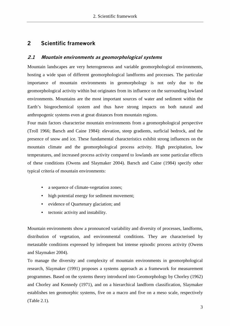
Caine (1974) has illustrated this relationship for the flow of sediment in alpine environments
(Figure 2.1).
Figure 2.1 Caine’s alpine sediment cascade model (Caine 1974)
This sediment flux model depicts some basic internal components of a valley subsystem,
together with input and output relationships. Main sources of sediment in this slope subsystem
are the exposed bedrock and the atmosphere that introduces aeolian sediments. The elements
of this system are interconnected landforms located along an altitudinal gradient, which
provides the energy for sediment movement. The output from this subsystem is delivered into
the adjacent subsystem that takes up the sediment. In a mountain environment this could be a
low-order valley, a lake basin, or the ocean. The valley subsystem can be modified in
different ways according to the scale of investigations. Otto and Dikau (2004) identify four
sedimentary subsystems in the Turtmann Valley: (1) the hanging valleys, (2) the main
glaciers, (3) the main valley trough slopes and (4) the main valley floor (Figure 2.2). Each of
these subsystems contains its own set of sediment transport processes and storage landforms.

2. Scientific framework
6
Figure 2.2 Meso scale sediment flux model of the Turtmann Valley (Otto and Dikau 2004)
Geomorphological processes link the landforms of the sediment cascade. Consequently, Caine
(1974) uses a functional classification approach and distinguishes four process systems in
mountain environments:
1. The glacial system:
Frozen water in form of snow and ice occupies the highest elevations within mountains.
However, glacier movement can extend the location of the glacial system into lower
elevations, for example into valley floors or even towards the sea. The important role of
glaciers for sediment production derives not only from their enormous erosive force, but
also from the storage and release of water. Glacierised mountain environments produce
the highest denudation rates in the world (Caine 2004).
2. The coarse sediment system:
Coarse sediment is produced at cliffs and rock walls, creating typical depositional
landforms like talus slopes, mass movement deposits or rock glaciers. Mainly
gravitational processes like rock falls, landslides, avalanches and debris flows operate the
sediment movement. Steep gradients, high potential energy and increased weathering
favour mass movement processes and enable the production of coarse sediment. Where
process activity and intensity are high coarse sediment is transferred into rivers, thus
coupling slopes to channels. However, if local terrain conditions or reduced process
activity hamper the slope-channel coupling, the coarse sediment can be trapped within the
subsystems (Otto and Dikau 2004).

2. Scientific framework
7
3. The fine-grained sediment system:
The fine-grained sediment system is dominated by the activity of fluvial processes that
remove the material from its provenance area. Weathering and soil erosion, as well as
aeolian sedimentation are the main sources for fine-grained sediment.
4. The geochemical system:
Geochemical denudation is linked with solution weathering, nivation and fluvial
processes. Though chemical denudation rates are usually lower compared to mechanical
denudation, the importance of the geochemical system is increasingly realized (Rapp
1960; Owens and Slaymaker 2004).
Two main factors govern the intensity and efficiency of sediment transport in the three later
systems: bedrock and surficial geology and the basin’s topographical characteristics i.e. the
size, relief and landsurface structure (Owens and Slaymaker 2004). Though Caine’s (1974)
classification is a functional approach, the different sediment systems imply an altitudinal
differentiation of mountain areas. Glacier and coarse sediment systems most often cover
higher altitudes, while fine-grained and geochemical systems typically occur in valley floors
and at lower elevations.
A purely topographic classification of mountain environments is given by Fookes et al.
(1985). Their “mountain model” includes five zones, each associated with typical landforms,
material and processes (Figure 2.3) located at different altitudinal levels of the mountain
system.

2. Scientific framework
8
Figure 2.3 Mountain Zones by Fookes et al. (1985). Zone: 1 – High altitude glacial and periglacial, 2 – Free rock faces and associated slopes, 3 – Degraded middle slopes and ancient valleys floors, 4 – Active lower slopes, and 5 – Valley floors.
Focussing on geological and geotechnical aspects of mountain environments in the context of
road construction, Fookes et al. (1985) use the altitudinal zonation to distinguish surface
materials, denudation processes and landforms in each zone. Though one emphasis is set on
surface materials, additional information like average slope gradients are given as well.
The landforms within a sediment cascade often act as storages, where material is deposited for
a variable period of time. Shroder and Bishop (2004) identify five different storage
environments for non-volcanic mountains: (1) Nonglacial alpine and ablational valley floor
storage, (2) glacier and moraine storage, (3) terrace storage, (4) lacustrine and aeolian storage
and (5) channel and braided plain storage.
2.1.1 Time and space in mountain geosystems
Time and space plays an important role for sediment budget analysis. The scale dependency
of landforms with respect to time and space is widely acknowledged (Figure 2.4). The way in
which landforms are arranged in a landscape is termed a palimpsest (Chorley et al. 1984).
This term expresses a nested arrangement of objects of different age and thus creating a
hierarchy of landforms. The assemblage of different polygenetic landforms within a landscape

2. Scientific framework
9
is the result of different processes, which have been operating at different times or at different
phases, and with various intensities. Generally smaller and younger forms rest on top of larger
and older objects. Therefore, a landscape can contain different generations of landforms
(Büdel 1977), which represent different stages of evolution. In mountain environments these
generations almost always include imprints from former glaciations. In an alpine valley for
example, a hanging valley represents a large and old landform formed by several cycles of
Pleistocene glaciation in several hundred thousand years. The talus slopes, moraines and rock
glaciers, which are located within the hanging valley, were accumulated after the deglaciation
within a few hundreds or thousands of years only. On top of talus slopes processes like debris
flows or avalanches can operate within even shorter time scales (minutes, hours, years)
creating smaller landforms (debris cones, levees, avalanche tongues). Landform size interacts
with time; thus space and time have to be considered together (Massey 1999). This
assemblage of relict, overlap and replacement landforms (Hewitt 2002) in a landscape
exhibits how past processes still have an influence on today’s environments. On the one hand,
land surface variations and landforms created by past processes serve as a grounding,
boundary condition and regulator for current processes. On the other hand, deposits from past
processes act as sediment sources for subsequent processes.
Figure 2.4 Time and space scales in geomorphology (Brunsden 1996)

2. Scientific framework
10
Landforms of various sizes take different time to form and last for different lengths of time
before they are eroded away (Figure 2.4). Besides a spatial hierarchy, expressed in the size of
the landform, a temporal hierarchy of formative process events can be defined as well
(Brunsden 1996). The time scale of an event can be equated with the duration of the process
and the time required to generate a landform. Debris flows or rock falls are rapid events
operating on very short time scales of a few minutes or seconds, thus the resulting form may
be created very quickly. Sustained climate change, which caused for example the Little Ice
Age and associated large moraine complexes, has a significantly longer duration, e.g. several
hundred years. Orogeny takes several million years, thus operating on a time scales of a
different order of magnitude. The composition of landforms results from a constant
adjustment to environmental conditions, where variations within the adjustment represent
sensitivity towards change of a geomorphological system (Brunsden and Thornes 1979; Dikau
1998). Sensitivity is a function of coupling of processes and process-response between the
different system elements and is often associated with negative feedbacks.
The evolution of the land surface is generally regarded as a dynamic equilibrium, which
suggests that the system responds in a complex, linear manner to environmental changes or
random internal fluctuations that cause the crossing of internal thresholds in order to reach a
balance between the formative forces (Schumm 1979). Many concepts of landscape evolution
(cf. paraglacial landscape response, chapter 2.3.2) assume steady-state conditions, where
fluctuations occur around a mean equilibrium. However, this assumption is critically
questioned by Jordan and Slaymaker (1991) and Ballantyne (2003).
The dynamic equilibrium paradigm is challenged by the concepts of complexity and
nonlinearity, which give rise to a more chaotic and less predictable model of landscape
evolution (Phillips 2003). These concepts reduce the incidence of steady-state equilibriums in
nature through various types of non linear response. These include thresholds, storage effects,
saturation and depletion, positive feedback mechanisms (self-reinforcing), self-limiting
processes, competitive interactions, multiple modes of adjustment, self-organisation and
hysteresis (Phillips 2003). Complexity describes a system behaviour, which emerges from the
interaction of the system components (De Boer 2001). Emergent phenomena or properties
(landforms, structures, and reactions) appearing within complex systems that cannot be
immediately explained or predicted by simple interaction of the systems individual
components (Spedding 1997). These emergent properties only become apparent at a certain
level of system complexity, but do not exist at lower levels (Favis-Mortlock et al. 2000). In

2. Scientific framework
11
mountain environments the formation of moraines is an example of emergent structures. Two
conditions produce moraines: the creation of large amounts of debris through bedrock erosion,
and the transport and deposition of this material by the glacier, instead of removal by
glacio-fluvial processes. Thus, the debris production and deposition represent the emergent
results of interdependent variables, like bedrock topography, glacier dynamics or subglacial
drainage network (Spedding 1997). The sediment dynamics of a drainage basin can also be
regarded as an emergent property of the drainage basin system itself (Wasson 1996).
Although they result mainly from local, small-scale processes, sediment dynamics and
sediment yield cannot be explained by analysis of small-scale process alone (De Boer 2001).
Temporal and spatial scales, system configuration, complexity, and coupling also have to be
considered in mountain sediment budget analysis. Additionally, Jordan and Slaymaker (1991)
point out that the occurrence of events is another aspect that affects sediment budget models.
Sediment supply may be more or less constant or characterised by episodic or singular events.
Such behaviour affects the choice of time scales and methods of data gathering for sediment
budget studies (Jordan and Slaymaker 1991).
2.2 The sediment budget approach
A budget is the quantity of objects involved in or available for a particular situation. Hence, a
sediment budget is a summation of all the sediment within a landscape, or as Reid and Dunne
(1996) define it,
“ … an accounting of the sources and disposition of sediment as it travels from its point of
origin to its eventual exit from a drainage basin.”
This definition includes the main elements of sediment flux through a landscape, the sources,
the transfer processes and the sinks, where sediment is finally or temporarily deposited. The
sediment budget approach provides a framework for the analysis of landform and land surface
evolution. Additionally sediment budgets are useful tools for resource management,
especially when human impact on geomorphic systems is studied (Reid and Dunne 1996).
Various sources of sediment production exist for mountain environments. Slaymaker et al.
(2003) identify four sediment sources in mountains with a present or past glacial history:
1. fine-grained glacial deposits (rock flour) derived from subglacial erosion and located
in glacier forefields;

2. Scientific framework
12
2. fluvioglacial deposits derived from paraglacial valley fill and terraces from the early
Holocene;
3. fluvioglacial deposits derived from exposed glacier forefields and moraines during
neoglacial advances; and
4. sediments originating from hillslope instabilities.
In other words bedrock outcrops, hillslopes and glacigenic depositions of various ages are the
main sediment sources in mountain environments. Hence, weathering and glacial erosion are
the major processes that produce sediment. Gravitational, glaciofluvial and periglacial
processes often dominate sediment transport in the vicinity of the source area, while fluvial
processes are responsible for the reworking of intermediate storage, the discharge of material
from catchments and the final transfer to the sinks. The coupling between slopes and channels
governs the transport efficiency between source and drainage basin outlet (Caine and
Swanson 1989). Lakes and oceans are sinks for sediments excavated from mountains.
However, large volumes of sediment have accumulated in sedimentary basins and valleys.
Sedimentary basins are generally of tectonic origin, for example related to orogeny (Einsele
2000) and are filled over very long time scales (millions of years). Valleys are temporary
sediment sinks and store sediment until an environmental change allows a process, for
example glacier advance to remove the sediment from the valley.

2. Scientific framework
13
The principle of the sediment budget approach is the relationship between the input and the
output of a system:
SIO ∆−= (2.1)
O is the output of a system and I is its input, while S∆ is the change of storage within the
system. This principle describes the flow of sediment through a landform as well as through
an entire catchment. Changes in the relationship between I and O at specified temporal and
spatial scales indicate changing process activity, intensity and changing boundary conditions
within the system.
A quantification of the sediment transfer process is expressed by the sediment load (SL),
which is the amount of material that crosses a defined area per time unit. The sediment load is
commonly calculated for fluvial systems; however a sediment load of a glacier or a rock
glacier can be calculated as well. The measurement unit is tons per year (t/a).
The sediment yield (SY) describes the amount of sediment that is discharged from a drainage
basin in a specified period of time, usually looking at fluvial processes and focusing on the
suspended river loads. Sediment yield is also given in tons per year (t/a). SY is calculated
using the following equation:
TASVSY
d
bρ= (2.2)
Where SV is the volume of stored sediment, ρb is the dry bulk density of the bedrock, Ad is the
denudation area and T is the time period of sediment discharge.
The specific sediment yield (SYspec) includes a specific unit area in the sediment yield
calculation:
SYspec = SY / A (2.3)
Sediment yield is regarded as an indicator of erosion and sediment delivery of a drainage
basin, emerging from its geological history, the geomorphological setting and the climatic
regime (Schiefer et al. 2001). Specific sediment yield declines with increasing catchment size
(Milliman and Meade 1983; Chorley et al. 1984), indicating a scale dependency of this
parameter (Schiefer et al. 2001), and the negative influence of sediment storage within a

2. Scientific framework
14
catchment on the sediment yield. However, this relationship is not valid for formerly glaciated
drainage basins, as Church and Slaymaker (1989) have shown.
The sediment delivery ratio (SDR) is a dimensionless parameter describing the ratio between
sediment yield and total erosion for a catchment:
SDR = SY / E (2.4)
The SDR compares the amount of sediment that is actually transported from the sources of
erosion to the catchment outlet, to the total amount of material eroded from the same area
above the basin outlet. Various factors influence the SDR including slope length, basin
morphology, channel-hillslope coupling, dominant processes, to name just a few. Steep slopes
and channels, high relief, and drainage density tend to produce high SDR, whereas large
distances between sediment sources and channels, and low-gradients produce lower SDR
(Milliman and Syvistki 1992).
Erosion within a drainage basin is quantified by the denudation rate (DR), describing the
amount of material eroded per unit area over time. The DR dimension is usually mm a-1, or
mm ka-1. The corresponding depositional rate is the sedimentation rate (SR). The sediment
volume SV can be used to calculate the mechanical denudation rate DR.:
TA SV DR
ds
b
ρρ= (2.5)
This term includes the dry bulk density ρ of the sediment ρs and the bedrock ρb, the
denudation area Ad and the time period of deposition T. If the denudation area is bedrock only,
for example a cliff, the denudation rate is termed rock wall retreat rate. The rock wall retreat
rate can be calculated using equation 2.5 as well and has the same unit as the DR.
A combination of equations (2.2) and (2.5) allows calculating the sediment yield from the
mechanical denudation rate:
SY = DR ρs (2.6)
In practice, the construction of sediment budgets is a very complex task, challenged by the
difficulty of measuring exact rates, the understanding of process mechanics and the
quantification of storage elements. Additionally, transport and storage processes may vary in

2. Scientific framework
15
time and space. Very few works have studied the sediment budget over longer time scales, or
in form of monitoring programs. One of the most famous works was started by Rapp (1960)
in northern Scandinavia and is still partially continued today (Schlyter 1993; Gude et al. 2002;
Beylich et al. 2004).
Dietrich et al. (1982) give three requirements for sediment budget studies in order to integrate
temporal and spatial process variations:
1. recognition and quantification of transport processes;
2. recognition and quantification of storage elements; and
3. identification of linkages among transport processes and storage elements.
Hence, the foundation for all sediment budget studies following these three requirements is a
detailed geomorphological mapping campaign in order to identify the processes and storage
landforms. Based on this information linkages can be identified by the construction of a
qualitative sediment budget model (Dietrich and Dunne 1978). Figure 2.5 depicts the
qualitative sediment budget model for a hanging valley in the Turtmann Valley created by
Otto and Dikau (2004).
Figure 2.5 Qualitative sediment flux model of the Brändjitaelli hanging valley (Otto and Dikau 2004)

2. Scientific framework
16
2.2.1 Denudation rates and sediment yield
Denudation rates and sediment yields quantify the amount of land surface change in
geomorphic systems and represent an integral signal of the systems activity, connectivity and
configurational state. Sediment storage volumes are often used to calculate denudation rates
and sediment yields.
For larger drainage basins, denudation rates are estimated from sediment yield measured or
assessed in rivers or from lake or valley fill deposits at a catchment outlet (Owens and
Slaymaker 1992; Einsele and Hinderer 1997; Hinderer 2001; Schiefer et al. 2001). Some
studies have measured sediment yield in small catchments using sediment traps or nets placed
below slopes (Caine and Swanson 1989; Johnson and Warburton 2002; Krautblatter and
Moser 2005). Relief and drainage basin area are regarded as the major controlling factors for
sediment yield (Milliman and Syvistki 1992). Areas of high relief generally produce high
yields, while low yields are associated with lowland areas. A climatic control on sediment
yields is observable in different climatic zones. Precipitation and glacier occurrence strongly
influence sediment yields; consequently mountain environments affected by these two factors
often produce high sediment yields (Hallet et al. 1996). Lithology controls sediment yields to
a far lesser extent in mountain areas compared to precipitation and glacial erosion. However,
sediments and rocks especially sensitive to weathering, like loess, volcanic or alluvial
deposits, or mudrocks can produce increased levels sediment discharge from limited areas
where other variables remain equal. In contrast, protection from weathering by thick
vegetation cover or clayey soils hampers erosion and decreases sediment yields especially in
lowland areas. In alpine environments however, vegetation is often significantly reduced,
especially at higher elevations. Finally human activities strongly influence sediment yields,
expressed by increased soil erosion, earthworks in floodplains or reservoir construction
(Einsele and Hinderer 1997). Hence, high relief, strong climate variations, the presence of
glaciers and lack of vegetation cover are contributory factors for high sediment yields in
mountain areas.
However, the sediment yield provides only a rough approximation of the sediment budget, as
denudation, considered as bedrock retreat or surface lowering, is estimated for an entire
catchment, without local differentiation or respect to spatial and temporal scales. The
limitations of the sediment yield approach have been stressed by various authors (Phillips
1986; Harbor and Warburton 1993). When derived from sediment yield data, denudation rates
are only valid when no change in storage occurs (Phillips 1986). This limitation underlines the
importance of sediment storage, but as well stresses the close relationship between time scales

2. Scientific framework
17
and denudation rates. Temporal variations in the denudation rate together with the effect of
storage have a strong impact on sediment yield. These influences can be averaged out, when
the time span of the sediment yield measurement is extended and both storage and release of
sediment are included in the denudation rate estimation. However, extreme events, periodic
phenomena or major environmental changes can influence drainage basins over longer time
scales, thus altering the denudation rate (Phillips 1986).
2.2.2 Sediment budget and storage quantification
Early sediment budget studies have been carried out very often in lowland environments and
within small drainage basins (Dietrich and Dunne 1978). Jordan and Slaymaker (1991) point
out that for large glacierised mountain basins approaches used in lowlands cannot be applied,
because of entirely different conditions in mountain environments. Due to the highly episodic
nature of mountain geomorphological processes steady-state models, often used in lowland
budget approaches are not appropriate for mountain regions (Jordan and Slaymaker 1991).
Early work on alpine sediment budget quantification was done by Jäckli (1957) and Rapp
(1960). Jaeckli (1957) produced the first sediment budget in the Alps for the upper Rhine
catchment. He included all major processes in his sediment flux quantification and concludes
that about 80 % of the sediment movement is done by fluvial processes. Rapp (1960)
investigated sediment movements and storages in the Kärkevagge valley in northern
Scandinavia over a period of more than ten years. His results indicate that coarse debris and
bedrock slopes are the most important elements of the sediment flux system, contributing
about 60 % of the sediment budget, followed by soils mantled and fine sediment slopes with
30 %. Barsch (1981) investigated the sediment flux in an high Arctic mountain valley in
Ellesmere Island, Canada. His studies indicate a dominance of fluvial processes (96 %)
followed by glacier erosion (2 %) and rock fall processes (1 %). Though other erosional
processes like solifluction, debris flows or slope wash operate on large areas, they make only
minor contributions to the sediment flux of this region.
Caine’s intensive work in the Colorado Rocky Mountains (USA) produced sediment budgets
for three small mountain catchments. His results for William Fork, Eldorado Lake and Green
Lakes Valley showed that talus shift and rock glacier flow (only Green Lakes valley) are the
most effective processes within the coarse debris system, moving more than 90 % of the
available material. Soil creep and solifluction dominate the fine sediment system making up
over 90 % of total fine debris movement (Caine 1986, 2001).

2. Scientific framework
18
Jordan and Slaymaker (1991) investigated sediment movement and storage along several
reaches of the Lillooet River (British Columbia, Canada) and compared these quantities with
the sediment yield from the basin. Storage volumes were estimated from field investigations
and average thickness values, process activities were taken from the literature. Debris flows,
glaciers and landslides are the most important sources of sediment in this basin; however,
Jordan and Slaymaker detected sediment originating from human activities like logging and
agriculture in the basin fill as well. Most of the sediment is stored in landslide deposits (>
70%), the floodplain (> 20%) and in fans (> 2%). They conclude that the estimated sediment
supply from the different sources is not balanced with the observed long-term sediment yield
from the basin. Their conclusions led to a modification of the paraglacial concept by Church
and Ryder (1972) (cf. chapter 2.3.2).
The constraints on denudation rate assessment from sediment yield show that estimation of
storage volumes is the crucial element of all sediment budget analysis. Various methods are
applied in order to estimate sediment storage in mountain environments. Fundamental
geomorphological methods like mapping, topographic survey and photogrammetry are the
most basic methods and hence frequently used (Jäckli 1957; Rapp 1960; Jordan and
Slaymaker 1991; Watanabe et al. 1998; Curry 1999).
Though not included in a sediment budget, Barsch (1977a; 1977b) estimated the storage
volume of rock glaciers in the Swiss Alps. Based on air photo mapping he used different
thickness scenarios to calculate a volume of 0.8 to 1.4 km³ of coarse sediment stored in active
rock glaciers. Referring to numbers given by Jaeckli (1957), Barsch (1977a) concludes that
active rock glaciers transport around 20% of all mass-wasting processes with an estimated
denudation rate of 2.5 mm a-1. In the Turtmann Valley, Nyenhuis (2005) applied Barsch’s
approach to assess rock glacier volumes. He estimated between 0.05 and 0.07 km³ of rock
glacier volume.
With the availability of digital elevation models (DEM), simple geometric forms representing
actual landform shapes are used to estimate storage volume, for example a half-cone
representing a talus cone landform (Shroder et al. 1999; Campbell and Church 2003).
Following geomorphometric approaches for glacial valley description (Graf 1970), quadratic
or power-law equations have been applied to cross-sections of glacial valleys in order to
estimate valley fill deposits (Hoffmann and Schrott 2002; Schrott and Adams 2002; Schrott et
al. 2003). However, this method compared to geophysical data on sediment thickness in

2. Scientific framework
19
valley bottoms, tends to overestimate sediment volumes and can only be used as a rough
estimation (Schrott et al. 2003). A new approach to estimating sediment volumes based solely
on DEM data is introduced by Jaboyedoff and Derron (2005). Their interactive routine,
named Sloping Local Base Level (SLBL) is based on geometric assumptions about the glacial
trough shape. Using this technique, they calculated a volume of 118 km³ sediment for the
upper Rhone Valley, which correlates well with the available geophysical information on
sediment thickness (cf. chapter 3.3.2).
Occasionally, sediment coring has been applied to determine sediment volumes (Schrott and
Adams 2002; Schrott et al. 2002). However, this method is restricted to very few landforms in
mountain environments, like flood plains and alluvial deposits, due to technical difficulties
and associated high costs evoked by remote locations and subsurface materials characteristics.
The use of geophysical investigation techniques becomes increasingly important for the
quantification of sediment storage, especially in rugged mountain terrain. Non-destructive
geophysical methods permit a faster and often less expensive acquisition of high-resolution
data on structure and composition of storage landforms compared to other methods such as
drilling. Geophysical investigations on storage landforms are applied on two spatial scales,
governed by expected sediment thickness and the penetration depths of the applied method.
Large scale investigations often use the seismic reflection method and strong seismic sources,
such as explosives or weight droppers, or gravity surveying, enabling bedrock detection at
several hundred meters of depth. These surveys are applied to quantify sedimentary fills of
large valley systems or other sedimentary basins. The operating expense, both in time and
cost, for seismic reflection surveys of this scale are very high compared to small scale
investigations. Therefore, very few investigations of this size exist. The major valleys in the
Swiss Alps have been investigated in this way within a National Research Program (Pfiffner
et al. 1997b). Seismic reflection and gravity survey have been applied along several transects
in the Rhone Valley (Figure 2.6) between Brig and Lake Geneva (Finckh and Frei 1991;
Besson et al. 1992; Pfiffner et al. 1997a; Rosselli and Olivier 2003). Sediment thicknesses
between 300 and 900 metres have been detected, and a total mass of 106.2 km³ stored
sediment was calculated for this part of the Rhone Valley based on these surveys (Hinderer
2001). A similar study, but on a different scale has been carried out by Froese et al. (2005),
who investigated a 1000 km long reach of the Yukon River in North America. They detected
a sedimentary fill between 8 and 30 m in depth using ground penetrating radar and resistivity

2. Scientific framework
20
sounding. However, this study does not focus on the sediment budget, but rather uses
floodplain stratigraphy to interpret the equilibrium state of the river.
Figure 2.6 Cross profile through the Rhone Valley derived from seismic reflection surveying at Turtmann (Finckh and Frei 1990)
Small scale, shallow geophysical investigations require much less effort and are more
frequently applied. The most common methods include seismic refraction (SR), electric
resistivity tomography (ERT), and ground penetrating radar (GPR) (for a more detailed
description of these methods cf. chapter 3.2). Talus slopes are the most frequently studied
landforms in alpine environments using geophysical methods. Quantified talus volumes are
frequently used to calculate a retreat rate of the adjacent rock walls (Sass and Wollny 2001,
Schrott and Adams 2002, Hoffman and Schrott 2002, Sass 2006).
Sass and Wollny (2001) used GPR to determine thickness and internal composition of talus
slopes in the German Alps. They detected the regolith-bedrock boundary at depths between 5
and 15 metres below the surface, referring to rock wall retreat rates of 0.1 mm a-1 for the
Holocene. Schrott and Adams (2002) applied seismic refraction and resistivity soundings,
combined with coring and C14 dating to quantify the sediment storage volume in an Alpine
basin in the Dolomites, Italy. They derived sediment thicknesses in the glacial trough of 15 to
72 m and a total volume of 0.35 km³ for a 17 km² sized valley. Their best estimate of volume
results in a denudation rate of 1.1 mm a-1. Investigations by Schrott et al. (2002; 2003) in the
Reintal, Germany, can be regarded as the most detailed application of geophysical methods in
a single glacial trough valley in the northern European Alps. A total of 66 geophysical
soundings have been carried out on various storage landforms including talus slopes, debris
cones, avalanche deposits, alluvial fans and floodplain deposits. Talus slopes and talus cones

2. Scientific framework
21
store more than 70 % of material in this catchment. For talus slopes a mean regolith
thicknesses between 3 and 23.5 m was determined (Hoffmann and Schrott 2002) using
seismic refraction, resulting in a rock wall retreat rate of 0.5 mm a-1. A combination of the
geophysical surveys, detailed geomorphological mapping of storage landform including
process activity, coring along the valley floor and C14 dating allowed for the construction of a
detailed sediment budget and enabled conclusions to be drawn about the paraglacial evolution
of the Reintal (Schrott et al. 2002). The backfilling volume of a small alluvial sink, produced
by a landslide event, was calculated to be 0.9 million m³, with a mean sedimentation rate
between 18 and 27 mm a-1.
2.3 Evolution of mountain landscape systems
2.3.1 Uplift and erosion of mountains
The influence of tectonics and climate on long-term sediment fluxes is currently discussed
avidly in earth sciences, fuelled by new dating methods like cosmogenic nuclides (Peizhen et
al. 2001; Schaller et al. 2001; Kuhlemann et al. 2002; Molnar 2004; Nichols et al. 2005).
Mountains are the result of complex interactions between tectonics, climate and surface
processes. Plate tectonic processes, causing orogeny, are responsible for most of the world’s
highest mountains. According to the plate setting and the tectonic process, divergence or
convergence, different types of orogeny produce different mountain types. Ocean-to-continent
plate margins lead to the formation of continental margin building orogens, like the Andes for
example. Continent-to-continent plate margins create collisional mountains like the Alps or
the Himalaya (Huggett 2003; Slaymaker 2004). When crustal material is accumulated in the
orogenic wedge the surface is elevated. In case of a collisional orogeny for example, material
from the continent crust and the ocean crust gets deformed, uplifted and finally exhumed.
These processes produce the complex lithologic conditions of stacked, folded and overlapping
lithologies which characterise mountains.
For a long time erosion was believed to be the opponent to uplift. Advanced understanding of
interaction and feedbacks between tectonics, isostasy, climate and erosion processes tackles
this belief and produces a far more complex image of mountain evolution (Pinter and Brandon
1997). This new perspective on mountain evolution is studied in the field of tectonic
geomorphology (Burbank and Anderson 2005),a research field located at the interface
between geomorphology, geophysics and sedimentology (Summerfield 1996). The effect of
erosion on uplift rate is generally discussed in close connection with the impact of climate on
2. Scientific framework
22
mountain building and regarded as a feedback system (Molnar and England 1990;
Summerfield and Kirkbride 1992; Molnar 2003). Erosion of sediment, strongly influenced by
climatic conditions, represents the removal of material from one area. Due to isostatic
response, this removal of material leads to tectonic uplift, as load from the earth’s mantle is
relieved (Molnar and England 1990). Thus, erosion could lead to mountain building. The
system feeds back when surface uplift perturbs regional climate conditions, leading to
increased erosion rates (Summerfield 1996).
Schlunegger and Hinderer (2001) studied the correlation between erosion and uplift in the
central Swiss Alps. They infer a positive feedback between surface erosion and tectonic
forcing for the drainage basins of the rivers Rhone and Rhine. In these two basins both
present-day sediment yields and uplift rates are significantly higher compared to other
drainage basins in the study area. This correlation is interpreted as a response of the earth’s
crust to locally increased surface erosion rates through enhanced uplift rates combined with
frequent earthquakes. For the same area, Bansemer (2004) suggests that uplift and erosion are
in a dynamic equilibrium on a long-term scale (5 Million years). Based on a multiple
regression of geomorphometric landform parameters, uplift and erosion rates, he showed how
rock failure and gravitational mass movements compensate for tectonic uplift in the Swiss
Alps. A correlation between Quaternary snowlines, as a proxy for Pleistocene glaciation, and
geomorphometric parameters provided an alternative model of steady-state conditions for the
Swiss Alps. Hence, Bansemer (2004) concludes that mechanical rock properties and high
erosion rates induced by Quaternary glaciation are the controlling factors governing the height
of Alpine peaks in Switzerland.
Various numerical models exist to simulate the evolution of mountain landscapes (Tucker and
Slingerland 1996; Kühni and Pfiffner 2001; Schlunegger and Hinderer 2001). These models
generally focus on the influence of surface processes on the landsurface evolution and its
relationship to tectonic activity. Kühni and Pfiffner (2001) use a surface process model to
reproduce different patterns of uplift combined with the evolution of drainage networks in the
Swiss Alps. Tucker and Slingerland (1996) model the rate of sediment flux into a foreland
basin, in order to understand the functional relationship between the sediment volumes
expelled from a mountain area and the assumed independent variables like relief and climate.
They conclude that sediment storage, in this case located in an intramontane basin caused by a
drainage basin being cut off through a rising thrust, produces a mismatch between the tectonic
event and the timing of sediment delivery to the foreland basin.
2. Scientific framework
23
In order to investigate the main tectonic and climatic impacts on long-term sedimentation
from the European Alps to the surrounding sedimentary basins, Kuhlemann et al. (2002)
construct a sediment budget for the entire European Alps. Based on stratigraphic data of
sedimentary basin fills, they estimate volumes of sediment excavated from the mountain
range since the onset of its existence. Kuhlemann et al. (2002) identify several phases since
the Oligocene of increased discharge rates into the basins, which are associated with possible
climatic or tectonic controlling factors. This sedimentologic approach differs strongly from
the geomorphological sediment budget approach, in terms of the significantly larger spatial (>
250,000 m²) and temporal (> 30 Ma) scale addressed.
2.3.2 The paraglacial sedimentation cycle
Specifically contrasted to the term periglacial, paraglacial sedimentation defines “nonglacial
processes that are directly conditioned by glaciers” (Church and Ryder 1972). For mountain
environments Church and Ryder (1972) introduced the concept of paraglacial sedimentation
based on data from sedimentation studies in two areas in Canada affected by glaciation. They
showed to what extend glaciation disturbs fluvial denudation conditions in the alpine
environment. The paraglacial sedimentation concept describes how geomorphic systems react
to the impact of glaciation and how landforms recover and relax in the ensuing period.
The unifying condition, which underlies all geomorphological processes and landforms
affected by paraglacial sedimentation, is the release of glacially conditioned sediment
(Ballantyne 2002a). Glacier activity increases erosion rates (Hallet et al. 1996) and produces
large amount of debris that is stored in valley floors and on glacial trough slopes. Church and
Ryder (1972) note that this material has reached a position of stability with respect to the
glacial processes in various types of moraines at the ice margins. However, with respect to the
nonglacial processes, these deposits are in unstable or metastable conditions and sediment is
subsequently released from these sources by various processes. Processes such as debris
flows, glaciofluvial erosion, and rock avalanches caused by debuttressing of rock slopes after
deglaciation are considered to be the most important agents in the redistribution of sediment
in proglacial areas (Church and Slaymaker 1989; Cruden and Hu 1993; Ballantyne and Benn
1996; Curry 1999).

2. Scientific framework
24
Figure 2.7 The paraglacial model by Church and Ryder (1978)
Ballantyne (2002b) identifies six paraglacial landsystems with individual sets of landforms
and sediment facies. Paraglacial landsystems can be divided into primary and secondary
systems. Primary systems are directly glacially conditioned and the sediment involved has not
yet been reworked by non-glacial processes. These systems tend to be in the immediate
vicinity of glaciers. In contrast, secondary systems include not only the release of in situ
glacigenic material, but also a reworking of paraglacial deposits further from the glacier
(Ballantyne 2002b). These landforms can be regarded as storage components of an interrupted
sediment cascade with various primary sediment sources: (1) rockwalls, (2) drift-mantled
slopes, (3) valley floor deposits and (4) coastal deposits; and several sediment sinks: (1)
alluvial valley fill, (2) lacustrine deposits, (3) coastal / near offshore deposits and (4) shelf
deposits (Ballantyne 2002b).
The time span during which these paraglacial processes operate is termed the paraglacial
period (Church and Ryder 1972). This period starts when glacial sedimentation ceases and
ends, when glacially conditioned sediment sources are depleted, or when a steady-state in
relation to the reworking processes is achieved. The depletion of sediment sources with time,
as an integral element of the paraglacial cycle has led to the idea of exhaustion (Cruden and
Hu 1993; Ballantyne 2002a, b). Conceptual models of paraglacial sediment movement are
generally represented by a declining curve (Figure 2.7), describing the change of sediment
yield from an initial high level, at the onset of deglaciation, to a constant low yield towards
the end of the paraglacial period. The exhaustion model assumes steady-state conditions in
which no change occurs in the process mechanisms or boundary conditions. Of course this
assumption is highly speculative especially in mountain environments, as it pays no attention

2. Scientific framework
25
to episodic environmental changes like base-level changes, extreme events or human impact
(Ballantyne 2003). In the exhaustion model the paraglacial sediment release through time is
assessed by:
tat eSS λ−= (2.7)
Where St is the available amount of sediment at time t, Sa is the total available sediment at
time t = 0 and λ is the rate of loss of available sediment by either release or stabilisation.
For Sa = 1 at t = 0, λ is expressed as:
tSt −= /)ln(λ (2.8)
Thus, the rate of sediment release follows an exponential decline (Figure 2.8, Ballantyne
2002a), allowing for the estimation of remaining sediment available for release. The extent of
the paraglacial period spans from a few decades to some ten thousand years depending on the
spatial scale and the processes regarded (Church and Slaymaker 1989; Cruden and Hu 1993;
Harbor and Warburton 1993; Curry 1999; Ballantyne 2002a). This implies that paraglacial
sediment storage landforms may be accumulated, while at the same time other formerly
deposited landforms are eroded and vice-versa.
Figure 2.8 The paraglacial exhaustion model (Ballantyne 2002). Rate of sediment release (λ) is related to the proportion of sediment ‘available’ (St) at time (t) since deglaciation as tSt −= /)ln(λ .

2. Scientific framework
26
Church and Slaymaker (1989) elaborated this idea with respect to the sediment yield of
drainage basins of different sizes. In contrast to the conventional models, in which the specific
sediment yield declines as drainage basin area increases, they proved that for the rivers in
British Columbia (BC), Canada, sediment yield increased for larger basins. They conclude
that most of the sediment transported in the rivers originates from a remobilisation of valley
fill deposits, including river banks and the immediate valley sides. The material involved in
the remobilisation has been deposited in the valleys by Quaternary glaciation more than 10 ka
ago. With respect to the original concept of paraglacial sedimentation by Church and Ryder
(1972), Church and Slaymaker (1989) infer that the observed sediment yield of rivers in BC
still responds to the impact of deglaciation on the landsystem. Thus, they extended the
paraglacial period proposed from a few thousand years to more than 10 ka. This challenges
the traditional view on landscape evolution, where the sediment yield is considered to reflect a
denudation rate for a prevailing climate and regional geology. Emphasising the extraordinary
impact of Quaternary glaciation, they conclude that recent sediment yields are still a
consequence of these events, instead of reflecting Holocene erosion rates. However, the
impact of deglaciation, reflected by increased sediment yield, has shifted from the upland
catchments towards the major valleys (Figure 2.9).
Figure 2.9 The paraglacial sedimentation cycle modified by Church and Slaymaker (1989). The time scale spans approximately 10 ka.

2. Scientific framework
27
Church and Slaymakers model stresses the importance of sediment storage with respect to
sediment budgets and sediment yields in mountain landscapes and underlines the role of
relaxation time in systems (Schumm and Lichty 1965).
The distribution and arrangement of sediment storage can be regarded as a paraglacial
landform assemblage, in which landforms with the greatest formative longevity and
persistence dominate the landscape (Ballantyne 2003). Thus, after the deglaciation a
succession of landforms evolves from the initial setting of glacigenic landforms to post-
paraglacial landforms, where sediment is routed through different landforms representing the
sediment cascade. With respect to the role of sediment storage Ballantyne (2003) transferred
the original paraglacial model, where sediment yield is plotted against time since deglaciation,
to a model where sediment volumes decline with time (Figure 2.10). The volume of sediment
storage S at time t in Ballantyne’s model is defined as:
ttaa
ti eeSSeSS κλκ −−− −== )( (2.9)
where Si is the input of sediment, and κ the rate of sediment loss from the storage. A
calculation of the rate of sediment loss both from a storage landform κ and the entire basin λ
requires the total available volume of sediment Sa, which is usually not known. To overcome
this constraint Ballantyne states four prerequisite values: (1) the time since deglaciation at
which sediment volume achieved its maximum t’ ; (2) the time interval between deglaciation
and the present t’’ ; (3) the maximum volume of the sediment store Sm at t’ ; and (4) the present
volume of stored sediment Sv. Therefore, Sm and Sv can be calculated by:
'' )( ttaam eeSSS κλ −−−= (2.10)
And
'''' )( ttaav eeSSS κλ −−−= (2.11)
In order to calibrate this curve and solve the equations (3), (4) and (5), dating techniques
provide information regarding the time scale t’ and t’’ , while sediment volumes Sm and Sv can
be derived from geophysical surveying (Ballantyne 2003).

2. Scientific framework
28
Figure 2.10 Changing volume of sediment storage (Ballantyne 2003)
A first modification of the paraglacial model was introduced by Jordan and Slaymaker (1991)
while constructing a sediment budget for the Lillooet River in Canada. Their paraglacial
sedimentation model for this drainage basin allows for the impacts of episodic changes in
sediment input on the sediment yield (Figure 2.11). For the Lillooet River these changes result
from volcanic activity and associated debris flows and landslides as well as from human
intervention. Thus one constraint of the original model, the steady-state assumption is dealt
with in this approach. Harbour and Warburton (1993) include the variation of basin size into
the paraglacial concept, resulting in a suite of paraglacial sedimentation curves, with varying
relaxation times depending on the basin scale (Figure 2.12). This scale dependency has two
effects: (1) Basins of different size could experience the same sediment yield, and (2) the
relative magnitude of sediment yield for basins of different size will vary at different
measurement times.
Figure 2.11 Episodic impacts on the sediment input within the paraglacial cycle of the Lillooet River, Canada (Jordan and Slaymaker 1991)

2. Scientific framework
29
Figure 2.12 Model of paraglacial sediment yield for catchments of different size (Harbour and Warburton 1993)
The paraglacial sedimentation concept is the fundamental geomorphological model for
sediment flux and landscape evolution in mountain areas affected by glaciation. It underlines
the importance of sediment storage for mountain sedimentary systems with respect to
sediment delivery, sediment residence times and relaxation from the impact of glaciation.
However, many parts of these different paraglacial models need calibration and verification,
for which knowledge of volumes of stored sediment and timing of onset of deglaciation are
required (Ballantyne 2003). Today’s composition of mountain landscapes shows a dichotomy
of sediment movement. On the one hand intensified processes produce, transport and deposit
great amounts of material. On the other hand, once deposited, sediment stays immobile for
very long time in many places, because the forces necessary for remobilisation and transport
only operate occasionally (Church 2002). Typical examples of this situation are fluvial valley
bottom landforms, hanging valleys filled with talus cones and relict rock glaciers.

2. Scientific framework
30
2.4 Sediment storage landforms
The role of sediment storage within a sediment budget approach has already been stressed
above. Consequently, the sediment storage landforms within a catchment need to be
investigated. For alpine environments these are: slope storage landforms, glacial derived
landforms and fluvial derived landforms. In this study seven alpine landform types are studied
in detail: (1) talus slopes, (2) talus cones, (3) block slopes, (4) moraine deposit landforms, (5)
rock glaciers, (6) rock fall deposits, and (7) alluvial deposits. They are considered as the main
sediment storages in the hanging valleys of Turtmann Valley and can be regarded as the most
important storage landforms in many upper high mountain areas. These landform types will
be introduced here briefly focussing on their role within the sediment flux system. Fluvial and
glaciofluvial deposits have not been studied in detail here and are therefore not considered.
2.4.1 Talus slopes and talus cones
Talus slopes are valley-side slopes formed by the accumulation of debris at the foot of
rockwalls (Figure 2.13). Rockwall-talus systems are an important part of mountain
landscapes. Talus accumulations represent the first element in the sediment cascade that takes
up the input from the rockwall. Secondary processes acting on talus slopes such as periglacial,
or gravitational processes transfer the material into the next landform. In case of periglacial
creep the follow-up landform is a rock glaciers or protalus rampart. Processes related to talus
formation are regarded as azonal acting over a wide range of altitudinal and climatic zones
(Perez 1993). Rock fall as the main process has been studied in great detail (Rapp 1960; Caine
1967; Luckman 1976). Snow avalanches contribute to talus formation (Jomelli and Francou
2000) as well, but are also, together with debris flows and dry grain flows, responsible for the
remobilisation of talus material (van Steijn 2002). Ballantyne and Harris (1994) define
different types of talus slopes corresponding to the form of the talus body and the secondary
processes acting on them (Figure 2.14). Talus slopes are often well sorted with increasing
clast size downwards, caused by higher potential energy of larger clasts and sieving effects
towards the foot of the slope. Dry grain flows cause a movement of fines downwards leading
to a stratified internal structure of finer and coarser layers (van Steijn 2002) that is clearly
distinguishable in ground penetrating radar soundings (Sass 2006). Talus slopes are among
the most frequently studied landforms in geomorphology using geophysical techniques.
Consequently, comparably extensive information exists on sediment thickness and volumes of
these forms. Some thickness values are compiled in Table 2.

2. Scientific framework
31
Figure 2.13 Coalescing talus slopes at the entry to the Bortertaelli.

2. Scientific framework
32
Figure 2.14 Different talus slope types (Ballantyne and Harris 1994).
Table 2.2 Mean sediment thickness values from preceding studies.
Location Reference Method Mean sediment thickness
(m)
Bavarian Alps (GER) Sass and Wollny(2001) GPR 10-15
Lechtaler Alps (AT) Sass (2006) GPR, SR, ERT 25
Bavarian Alps (GER) Hoffmann and Schrott (2002) SR 7-23.5
South Wales (UK) Curry and Morris (2004) Geometry 5
Snowdonia, North Wales
(UK)
Sass et al. (subm.) GPR 8-10

2. Scientific framework
33
2.4.2 Block slopes
Straight slopes that are not located below bedrock walls will be termed block slopes in this
study (Figure 2.15). Various terms and theories exist about the formation of block slopes
including rectilinear slopes, Richter denudation slopes or debris-mantled slopes (Ballantyne
and Harris 1994). Two main theories exist on the formation of these slopes: (1) an earlier
theory by Richter (1901) and Lehmann (1933) interprets rectilinear slopes as the final stage of
parallel bedrock recession, with the former rockwall buried under the regolith (Bakker and
LeHeux 1952). Alternatively (2), these slopes are associated with periglacial conditions
(French 1996). Höllermann (1983) gives three prerequisites for the formation of rectilinear
slopes: (a) intensive, mostly mechanical in situ weathering, (b) lack of linear denudation
processes, and (c) no removal of debris at the foot of the slope. The regolith composition
spans from medium to coarse grained sand fractions to block size clasts. Following theory
two, rectilinear slopes can be proofs of former periglacial conditions, if a formation of in situ
weathering of underlying bedrock is demonstrated (van Steijn 2002). However, a combination
of these different ways of evolution is possible as well. Information on sediment thickness of
these slopes in alpine environments is scarce. Ballantyne and Harris (1994) give depths
between 0.6 and 3.5 m quoting several sources. As a lack of removal of material at the slope
foot is one prerequisite for the formation of rectilinear slopes, they are often decoupled from
sediment cascade. However, in the Turtmann Valley a coupling with periglacial creep
phenomena such as relict rock glaciers and gelifluction lobes can be observed.

2. Scientific framework
34
Figure 2.15 A block slope exposed to the south in the Hungerlitaelli.
2.4.3 Rockglaciers
Rock glaciers are periglacial landforms formed by creep of a mixture of sediment and ice.
They are defined as tongue- or lobe-shaped bodies that are separated from their surrounding
environment by steep frontal and side slopes (Figure 2.16). The state of activity is used as one
classification criteria: active (moving), inactive (not moving, but still frozen) and relict (not
moving, not frozen) (Barsch 1996). Other classification schemes differentiate lobate and
tongue shaped forms. Additionally, elongated protalus rock glaciers represent an early stage
in the landform development. Rock glaciers explicitly represent the continuum character of
landscapes as they develop from pre-existing landforms (Burger et al. 1999). According to the
debris source they are termed either talus rock glaciers or glacier-derived rock glaciers.
However, the transition between the original landform (talus slope, or moraine) is usually not
a sharp boundary, thus an exact discrimination of the onset of the rock glacier is not possible.
Within the alpine sediment cascade rock glaciers represent an important element in both
sediment movement and sediment storage (Jäckli 1957; Barsch 1977b; Barsch and Jakob
1998). When the sediment movement ceases, due to lack of gravitational forces, sediment
input or decrease of ice content, rock glacier often persist as relict landforms in a landscape
for a very long time, for example more than 10 ka (Frauenfelder and Kääb 2000), thus being
decoupled from input and output processes. The determination of rock glacier thickness is a
complicated task, especially applying geophysical techniques. Due to similar physical

2. Scientific framework
35
characteristics of ice and bedrock and the internal composition, i.e. a mixture of large blocks
and fines, ice and air, the lower boundary is often not detected. Table 2.3 gives a summary of
rock glacier thicknesses found in the literature, a more extensive list of which has been
compiled by Burger et al. (1999). In order to assess the sediment volume of a rock glacier the
internal composition and the ice content needs to be considered. According to borehole
information the ice content can vary considerably (Arenson et al. 2002). Ice contents are
generally considered to be between 50 and 70 % for active rock glaciers (Barsch 1977b;
Barsch 1996; Haeberli and Vonder Mühll 1996; Burger et al. 1999; Humlum 2000; Ikeda and
Matsuoka 2006).
Figure 2.16 Active rock glacier in the Hungerlitaelli.

2. Scientific framework
36
Table 2.3 Compilation of rock glacier thickness from literature.
Location Reference Method Rock glacier thickness (m)
Swiss Alps (CH) Barsch (1977a) Estimation based on height of frontal lobe
30-100
Khumbu Himalaya (IND) Barsch and Jacob (1998) Estimation based on height of frontal lobe
11-41
Himalaya, Karakorum (IND, PAK)
Owen and England (1998) Estimation > 15
Various Burger et al. (1999) Various 8-120 Swiss Alps (CH) Ahrenson et al. (2002) Borehole drilling > 63 Turtmann valley (CH) Nyenhuis (2005) Estimation based on height of
frontal lobe 3-38
2.4.4 Moraines
Moraines are landforms created by the direct action of glaciers. Due to the enormous erosive
forces of glaciers (Hallet et al. 1996), glacier deposits often dominate presently and formerly
glacierised mountain landscapes (Figure 2.17). Moraines are classified into ice-marginal,
subglacial and supraglacial types. Thus, moraine deposits are stored in different landforms
and locations. Ice-marginal accumulations form longitudinal ridges of lateral and terminal
moraines around the glacier margin with heights up to a few hundred metres. Subglacial
deposits cover the formerly glacierised surface as sheets of till, often creating a hummocky
surface. Supraglacial till is usually delivered to the glacier margin as medial moraines and
contributes to ice-marginal deposits (Benn et al. 2005). Additionally, melting waters remove
large amounts of till from the glacier bed and margin, which are accumulated below in valley
fills and lacustrine sinks. Sediment thicknesses of trough valley fills have been investigated
by various authors on different scales (Hinderer 2001; Schrott and Adams 2002, cf. chapter
2.2.2). However, little is known about glacial deposits of small cirque glacier in hanging
valleys. Sass (2006) investigating talus landforms in the Parzinn cirque, Austria, determined
the thickness of some adjacent moraine ridges to be between 10 and 24 m. Within the
sediment cascade, glaciers represent an important primary sediment source, while glacial
deposits act as secondary sediment sources, when a remobilisation of these deposits starts
after deglaciation (cf. chapter 2.3.2).
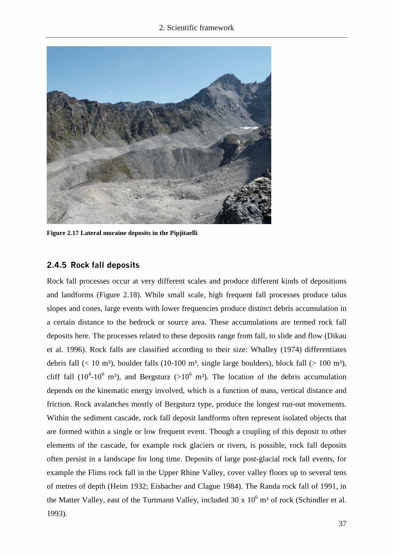
2. Scientific framework
37
Figure 2.17 Lateral moraine deposits in the Pipjitaelli
2.4.5 Rock fall deposits
Rock fall processes occur at very different scales and produce different kinds of depositions
and landforms (Figure 2.18). While small scale, high frequent fall processes produce talus
slopes and cones, large events with lower frequencies produce distinct debris accumulation in
a certain distance to the bedrock or source area. These accumulations are termed rock fall
deposits here. The processes related to these deposits range from fall, to slide and flow (Dikau
et al. 1996). Rock falls are classified according to their size: Whalley (1974) differentiates
debris fall (< 10 m³), boulder falls (10-100 m³, single large boulders), block fall (> 100 m³),
cliff fall (104-106 m³), and Bergsturz (>106 m³). The location of the debris accumulation
depends on the kinematic energy involved, which is a function of mass, vertical distance and
friction. Rock avalanches mostly of Bergsturz type, produce the longest run-out movements.
Within the sediment cascade, rock fall deposit landforms often represent isolated objects that
are formed within a single or low frequent event. Though a coupling of this deposit to other
elements of the cascade, for example rock glaciers or rivers, is possible, rock fall deposits
often persist in a landscape for long time. Deposits of large post-glacial rock fall events, for
example the Flims rock fall in the Upper Rhine Valley, cover valley floors up to several tens
of metres of depth (Heim 1932; Eisbacher and Clague 1984). The Randa rock fall of 1991, in
the Matter Valley, east of the Turtmann Valley, included 30 x 106 m³ of rock (Schindler et al.
1993).

2. Scientific framework
38
Figure 2.18 Rock fall deposit in the Niggelingtaelli
2.4.6 Alluvial deposits
Alluvial deposits are fluvially transported accumulations of fines deposited at flat, usually
lower locations in the hanging valleys (Figure 2.19). The sediments deposited here originate
from all of the other storage landforms. The locations of alluvial deposits may often include
small shallow lakes, formed from dead ice bodies after deglaciation. Depending on the size of
these lakes a complete filling with alluvial sediments is observable. However, these locations
are generally rare in upper high mountain areas, thus alluvial deposits play only a minor role
in the sediment cascade analysed here. In the Reintal, German Alps, Schrott et al. (2003)
measured a sediment thicknesses of 3-10 m for the alluvial valley floor fill.

2. Scientific framework
39
Figure 2.19 Alluvial deposit have almost filled up a small lake the Niggelingtaelli
3. Methods for sediment storage analysis
40
3 Methods for sediment storage analysis
3.1 Geomorphological system and land surface pattern analysis
The land surface is a patchwork of natural and man-made elements of different form and
material. This patchwork often reveals some kind of pattern, following a certain configuration
or structure. A structure is defined as “the way in which the parts of something are connected
together, arranged or organised” (Oxford Advanced Learners Dictionary 2006). The
distribution pattern or structure of landforms within a landscape emanates from its evolution,
conditioned by climatic, lithologic boundary conditions and human impact. Production,
movement and storage of sediment within a sediment cascade create landform patterns.
Landscape structure is frequently analysed in landscape ecology studies, where distribution
patterns of ecological environments, for example plant habitats, are quantified (Blaschke
2000). Numerous indices have been developed in order to describe the distribution structure,
neighbourhood relationships and spatial configuration of objects in an area (Haines-Young
and Chopping 1996; McGarigal 2002). In geomorphology the distribution of patterns and
relationships of geomorphic objects within a landscape is analysed, but approaches differ
from those applied in landscape ecology studies. Many analyses of geomorphological
landscape structure focus on geometrical patterns on the land surface, rather than on patterns
of process, landform or process domain distribution. Mutual to most of the geomorphometric
approaches is the development of an analytical taxonomy of land surface units, for example,
by Penck (1894), Kugler (1974), Speight (1974) or Dikau (1988). An overview of different
taxonomies can be found in Rasemann (2004). Land surface units are commonly classified in
a hierarchic way. Smallest units (form facets) have homogenous geomorphometric parameters
(slope, aspect, and curvature), larger units (form elements), which are composed of the
smaller ones, only have homogenous curvature characteristics (Dikau 1989). These units can
be derived by geomorphometric analysis using different approaches (Dymond et al. 1995;
Schmidt et al. 2003; Schmidt and Hewitt 2004). A very extensive list of landform elements is
given by Speight (1990). However, landform units in a geomorphometric sense often only
represent parts of the land surface and only very basic, mostly erosional landforms. Most
sediment storage landforms are not detected by geomorphometric analysis only, because
process and material of the landform is not considered in a purely geomorphometric approach.
Thus, a geomorphometric land surface classification is not sufficient for a landform structure
analysis (Dehn 2001).

3. Methods for sediment storage analysis
41
The concept of geomorphological mapping represents a more holistic approach towards the
geomorphic landscape structure analysis, taking into account both geometric and functional
characteristics, as well as neighbourhood relationships of landforms within a landscape. The
geomorphological map is a very complex tool to systemise a landscape and its
geomorphological components. It represents key elements of the geomorphological system,
serving as an inventory of landforms, subsurface material, observed recent processes and
inferred past processes at different scales. Based on this inventory the structure of a
geomorphological system and emerging pathways of sediment transfer can be studied in
detail.
Geomorphic mapping traditionally is done in the field. Owing to advances in remote sensing
and GIS technology many geomorphological maps are now often produced digitally, with or
without a field mapping campaign included. First attempts to automatically derive landforms
using digital elevation and remote sensing data have proved to be very successful (van
Asselen and Seijmonsbergen; Schneevoigt and Schrott 2006). Recent developments in semi-
automated digitizing tools make use of three-dimensional visualisation techniques and high
resolution elevation and remote sensing data, in order to accelerate and improve the quality of
landform mapping on a screen (Schneider and Otto in press).
Legends and guidelines for geomorphic maps differ from country to country. A review of
different geomorphical mapping systems can be found in Rothenbühler (2003), recent
mapping concepts are presented by Gustavsson et al. (2006) and Seijmonsbergen and de
Graaff (2006). In Germany guidelines for geomorphological mapping at large scales
(1:25,000 and 1:100,000) scale have been developed by Kugler (1964) and within a national
geomorphological mapping research programme (Stäblein 1980). A 1:25,000
geomorphological map of the Turtmann Valley is used in this study for the identification of
sediment storage landforms (Otto and Dikau 2004). At this scale information is often
generalised for cartographic reasons, which restricts resolution and therefore the ability to
discriminate between landforms. Therefore, the geomorphological map of the Turtmann
Valley, together with High Resolution Stereo Camera (HRSC) data (aerial photographs,
digital terrain model (DTM)) served as a basis for the detailed mapping of storage landforms,
which have been digitised as polygons with sharp boundaries and stored in a GIS database.

3. Methods for sediment storage analysis
42
3.2 Landform classification
A classification of landforms implies different attributes that not only describe individual
characteristics, but also reveal information about patterns of distribution and relationships
between the landforms. Dikau (1989) divides these attributes into primary and secondary
attributes (Table 3.1). Primary attributes include only geomorphometric parameters such as
slope, aspect or curvature, and represent derivates of the elevation data. Secondary attributes
refer to the position of the landform relative to the surrounding environment, shape, material,
and the geomorphodynamic and geomorphogenetic processes responsible for the landform
evolution. An extensive list of primary and secondary landform attributes that can be
calculated from a DTM was compiled by Huggett and Chessman (2002).
Table 3.1 Primary and secondary landform attributes (Dikau 1989)
Primary Attributes Secondary Attributes
• Slope • Aspect • Curvature
• Position in relation to the hierarchically higher-level unit • Type of toposequence • Height • Distance to the drainage divide • Distance to the drainage channel • Height difference to the drainage channel • Shape • Type and association of superimposed forms • Subsurface material • Geomorphodynamic processes • Geomorphogenetic processes • Geomorphochronology
3.2.1 Derivation of primary attributes
Primary attributes of the sediment storage landforms have been derived by geomorphometric
analysis of the HRSC data of the Turtmann Valley. The HRSC data contains a 1 m DTM and
multispectral imagery at 50 cm resolution (c.f. chapter 3.3). High resolution DTM data
combined with multispectral imagery provides a very detailed and useful basis for digital
landform mapping. However, high resolution can be an obstacle for geomorphometric
analysis as well. Small objects (< 2 m) produce a high degree of surface roughness, which
represents a factor of noise in the data. Derivates of elevation, such as slope, aspect or
curvature therefore contain information from smallest changes, for example a large boulder
(e.g. 5 m high) within an otherwise even surface. In order to remove this noise the 1 m DTM

3. Methods for sediment storage analysis
43
has been smoothed using a 7 x 7 pixel analysis window for the geomorphometric calculations
(slope, aspect, and curvature). This smoothing removes small systematic errors of the HRSC
DTM data as well (see chapter 3.2.3). The size of the analysis window was chosen after
comparing the results derived using different window sizes (3, 5, 7, 9). The 7x7 window
proved to be the most efficient in order to remove surface roughness and errors, but retain
important surface structure elements and the original altitude information.
Geomorphometric parameters are calculated according to Evans (1980). The implementation
of the interpolation algorithms into Arc/Info GIS was established by Schmidt et al. (2003)
using the Arc Macro Language (AML). This implementation provides not only different
algorithms for parameter calculations, compared to standard GIS software, but also allows a
definition of the analysis window size. A complete list of the algorithms used to calculate the
geomorphometric parameters can be found in Evans (1980) and Shary et al. (2002).
3.2.2 Derivation of secondary attributes
Secondary landform attributes represent not only the shape, material and formative process of
the landform, but provide information about the environmental setting and neighbourhood
relations around the landform. Therefore, they correspond to the geomorphological landscape
structure of an area. A relative location of the landforms within a hanging valley is expressed
by the distance to the drainage divide and drainage way. This parameter indicates the relative
position of landforms within the sediment cascade for example. These distances have been
calculated on a pixel basis using ridge data from the geomorphological map as drainage
divides and drainage ways from the digital topographic map 1:25,000 (Swisstopo).
A concept to study functional relationships and neighbourhood characteristics of landforms is
the idea of toposequences. Although, originally introduced to study patterns of landform
elements by Speight (1974), the concept can be extended to entire landform distribution. A
toposequence is a topographic succession of landforms or landform elements passed by a
virtual particle following gravitational forces through a landscape (Speight 1974; Rasemann
2004). Figure 3.1 shows the toposequence in arctic-alpine environments developed by
Stäblein (1984) for the mountains of Greenland. This example includes the entire
geomorphological set of processes, landforms and subsurface material found in an arctic-
alpine environment. However, no functional relationship between the elements of
toposequences is included in the toposequence approach. Not all neighbouring landforms
within a toposequence represent the real transportation route of sediment. Landforms can be
coupled or decoupled leading to sediment storage or sediment throughput and creating a

3. Methods for sediment storage analysis
44
neighbourhood relationship between the landforms. This functional relationship between
landforms, resulting from process activity, sediment flux and position leads to a landscape,
where the landforms are not distributed randomly, but reveal a distinct pattern of sediment
flux. Hence, a toposequence represents a sediment cascade, when sediment is transferred from
one landform to another. Time plays a strong role in this classification. Changing process
activity and intensity over time determine whether sediment is delivered from one landform to
the other and hence, whether a toposequence represents a sediment cascade or not. Landform
successions can temporarily become or stop being sediment cascades.
Up to now, no automatic procedure exists to derive toposequences from a digital dataset.
Rasemann (2004) notes that the identification based on quantitative criteria alone is not
enough to map toposequences. The formative semantic model of geomorphological objects
presented by Löwner (2005) provides a promising approach to the identification of
toposequences and sediment cascades. In additions to landforms he specifies coupling
processes to define valid functional relationships among landforms.
In this study, toposequences have been mapped manually based on the storage landform
database by linking each landform with its lower neighbour. Different typical toposequences
could be identified that led to the classification of toposequence types (cf. chapter 5.1).
Figure 3.1 Toposequence for arctic-alpine environments, Greenland (from Huggett and Cheesmann 2002, originally by Stäblein 1984)

3. Methods for sediment storage analysis
45
3.3 Topographical, digital imagery and geomorphological base data
A high resolution data set derived by the HRSC technique is used as elevation and imagery
base data. The “High Resolution Stereo Camera” (HRSC) sensor is a multi-spectral, stereo
scanner containing nine bands: one blue, one green, one red (tending to near infrared), one
near infrared and five panchromatic bands covering the green and red spectrum. It is a
pushbroom scanner consisting of CCD sensors in nine lines.
The HRSC data includes multispectral image of 0.5 m geometrical resolution and a 1 m DTM
that includes vegetation and buildings. DTM altitude accuracy is given with 10-30 cm. The
DTM data shows non random errors along overlapping swath locations. These errors are
represented by regular fabric-like structures that rise 10 - 30 cm above the surface (Rasemann
2004). The multispectral imagery is slightly blurred caused by different viewing angles colour
lines. This blur has been removed for the NADIR-channel, resulting in sharp black and white
images that served as the main aerial photo basis for geomorphological mapping. For more
information about the camera and dataset please refer to Neukum (2001).
The geomorphological map 1:25,000 of the Turtmann Valley is based on a field mapping
campaign during a preceding study by the author (Otto and Dikau 2004). Field maps of
1:10,000 together with aerial-photograph interpretation were used to produce the map within a
GIS environment. The mapping legend is based on the principles of the GMK 25 national
research program (Stäblein 1980). Geomorphic symbols have been taken from the mapping
legend for high mountains introduced by Kneisel et al. (1998). Modifications of the symbols
and the GMK25 principles have been made in order to adjust to the observed geomorphology.

3. Methods for sediment storage analysis
46
3.4 Methods for sediment storage quantification
Approaches towards a quantification of sediment storage volumes in alpine environments can
be divided into two spatial scales: (a) micro to meso scale, representing single landforms and
valley fill storage, and (b) meso to macro scale, representing sedimentary basin and lake fills.
While landforms on smaller scales act as intermediate storage on a medium time
scale (103-104 a), basin and lake fillings often serve as sediment sinks that are only depleted
by tectonic processes on very long time scales (105-107 a). Herein only micro to meso scale
objects are under consideration. In general, four different types of methods are applied to
assess the volume of sediment deposits on these different spatial scales (Table 3.3). However,
in this study only DTM analysis and geophysical surveying are used to asses the sediment
volumes.
Table 3.2 Methods and previous studies of storage volume quantification
Method Scale (acc. Dikau 1989)
Reference
Geometric approaches (valley cross profile, geometric objects, DTM analysis)
micro – macro Shroder et al. (1999), Schrott et al. (2003), Jaboyedoff and Derron (2005)
Geophysical surveying micro – meso Sass and Wollny (2001), Schrott and Adams (2002), Hoffmann and Schrott (2002)
Sedimentological analysis (stratigraphy)
meso – macro Schlunegger (1999), Hinderer (2001)
Drillings micro – meso Schrott et al. (2002)
3.4.1 Shallow subsurface geophysical investigations
Geophysical surveys measure the variation of some physical property of the lithosphere that
might reflect the subsurface geology. Various geophysical methods exist to investigate
underground characteristics such as geological structures, mineral deposits, fossil fuels,
underground water supplies, environmental, engineering or archaeological site issues (Kearey
et al. 2002). In contrast to investigation through borehole drilling, which provides only point
information, geophysical surveys deliver 2D or 3D information of the subsurface conditions.
Moreover, geophysical investigations are non-destructive, often more rapid and cost-effective
than drilling campaigns and usually represent the only possible method for underground
exploration in rough mountain terrain, where drilling is impossible due to, for instance
monetary or technical constraints. In general, geophysical methods can be divided into
techniques using natural fields of the Earth, such as magnetic or gravitational fields and

3. Methods for sediment storage analysis
47
techniques that require the input of an artificially generated energy into the ground, such as
seismic waves or electrical and electro-magnetic fields.
In geomorphology geophysical methods are used to study shallow subsurface features. In
alpine environments two main research fields make use of variations in physical subsurface
properties: (1) periglacial geomorphology (Berthling et al. 2000; Hauck 2001; Musil et al.
2002; Kneisel and Hauck 2003; Kneisel in press) and (2) sediment budget analysis i.e.
investigation of sediment storage bodies (Sass and Wollny 2001; Hoffmann and Schrott 2002;
Schrott and Adams 2002; Schrott et al. 2003). However, geophysical methods become
increasingly popular in other areas of interest in geomorphology, for example in landslide
studies (Sass et al. in press).
Although geophysical methods provide a comparably rapid way to investigate subsurface
conditions, an ambiguity in the interpretation of the results remains a major drawback. The
principle of geophysical techniques is based on knowledge of the internal structure and the
physical properties of the material under investigation. However, this information is generally
unknown and measured physical parameters, e.g. seismic wave velocity, are used to deduce
some internal structure. This problem is referred to as the inverse problem. Since physical and
chemical properties of rocks differ significantly in most cases no direct connection between
physical property and internal structure can be drawn. This ambiguity cannot be
circumvented, but an interpretation of the results is improved when different methods are
combined. Hauck (2001) gives a good introduction into the inverse problem.
This study makes use of changes in physical ground characteristics between the regolith
coverage and the bedrock base. Differences mainly derive from changing material density,
porosity and water/ice content. Seismic and electromagnetic radar waves as well as electric
currents are used to detect these differences. Thus, the methods applied here are: seismic
refractions surveying (SR), 2-dimensional electric resistivity tomography (ERT), and ground
penetrating radar surveying (GPR). These techniques will be briefly described in this chapter.
For a more detailed description of the methods and physical properties of subsurface materials
refer to geophysical textbooks (Knödel et al. 1997; Reynolds 1997; Kearey et al. 2002).
3.4.1.1 Seismic refraction (SR)
Seismic surveys measure the propagation of waves of energy through ground from a
controlled source. The application of an external impulse, for example a blow from a

3. Methods for sediment storage analysis
48
sledgehammer, creates an internal stress on the ground. Vibration of the rock or soil results in
a temporal deformation of the material. This strain manifests as a change in material shape
and size. Up to a certain level this strain is proportional to the applied stress leading to an
elastic deformation. Hence, the deformation is reversible and when the stress is removed,
strain is removed as well. The linear relationship between the stress and strain of a material is
determined by its various elastic moduli. Seismic waves are made up of the elastic strain that
propagates outwards from the source of stress.
Seismic surveys use the velocity of the seismic waves that travel through the ground. Two
types of waves are created depending upon the type of stress acting in the ground.
Compressional waves, also termed primary, longitudinal or p-waves, travel by compressional
strain in the direction of the wave. Shear waves, called secondary, transverse or s-waves,
propagate by a shear strain perpendicular to the wave direction. In general only the
propagation of the p-waves is used, because they are faster than s-waves, and therefore are
detected before the s-waves arrive. Typical p-wave velocities range between some hundred m
s-1 for loose debris to more than 6000 m s-1 for igneous or metamorphic rocks. In the
Turtmann Valley the bedrock velocities of the mica-shists and gneisses range between 2800
and 4000 m s-1 (Table 3.4).
Table 3.3 Geophysical properties of chosen subsurface material (different sources).
Material P-wave velocity (m/s) Resistivity (Ohm m) Water 1430 - 1590 10 - 300 Permafrost Ice 2500 - 4300 104 - 107 Glacier Ice 3100 - 4500 106 > 107 Clay 600 - 2600 1 -30 Talus deposits 600 - 2500 1000 > 20000 Till 1500 - 2700 500 - 3000 Schist 2700 - 4800 50 - 104 Granite 5500 - 6000 150 - 106 Talus debris 400 - 500 Moraine (Egesen) 600 - 900 Dolostone 3500 - 6000 5000 - 104
In the Turtmann valley: Mica-shists, gneisses (Pfeffer 2000, Knopp 2001)
2600 - 4000 2000 - 104
Mica-shists, gneisses (this study) 2900 - 4000 5000 - 7500 Mica-shists, gneisses (Krautblatter, subm.) - 2000 - 8000 (wet)
8000 - 18000 (dry) > 18000 (frozen)
Dry debris (Pfeffer 2000, Knopp 2001) 300 - 600 103 - 104 Compacted debris (Pfeffer 2000, Knopp 2001)
1100 - 2200 -
Dry loose debris (this study) 200 - 800 2000 - 5 * 105 Compacted debris (this study) 700 - 2000 - Frozen debris (Pfeffer 2000, Knopp 2001, Nyenhuis 2005)
1800 - 4000 104 - 106
Frozen debris (this study) 3500 - 4000 2 * 104 - 106

3. Methods for sediment storage analysis
49
If subsurface characteristics change at geological boundaries, the waves will be refracted at
the interface. While part of the energy is transferred into the deeper layer, some energy is also
reflected back towards the surface. The seismic refraction method makes use of the energy
refraction at subsurface boundaries, as waves of energy can be recorded at geophones at the
surface.

3. Methods for sediment storage analysis
50
The angle of incidence is equal to the reflection angle. The refraction angle follows Snell’s
law, which is:
21 /sin/sin VVri =θθ (3.1)
Where θi is the angle of incidence, θr the angle of refraction and V1 and V2 the seismic
velocities of the upper and lower layers, respectively. When the velocity of the lower layer is
higher than the upper layer, a critical refraction θc of the incoming wave occurs and the
refracted waves travel parallel to the interface with velocity V2. The critical refraction is given
by the ratio of the layer velocities:
21 /sin VVc =θ (3.2)
The resulting stress produces upward waves, called head waves that travel towards the surface
and may reach the geophones faster than the direct wave travelling at the velocity of the upper
layer (V1). Thus, one prerequisite for the seismic refraction method is an increase in velocity
towards deeper layers (V2 > V1). As the distance between the trigger location and the recording
geophone increases, the first impulses to arrive come from successively deeper layer
boundaries (Figure 3.2 A). First arrivals are recorded and time-distance plots are interpreted in
order to derive information on the depth of subsurface boundaries. In the case of a layered
subsurface structure, the first arrivals lie on a straight line (Figure.3.2 B). The first line
segment represents the travel-time of the direct wave, while the following segments are
associated with the underlying layers. The gradient of the travel-time segment represents the
reciprocal velocity of the layers, which is equal for both layers at the crossover distance Xcross.
The depth of the refractor can be calculated from the location of the intercept time ti, which is
the intercept of the travel-time segment with the time axis t:
21
2/121
22 )(2
vv
vvzti
−= (3.3)
Thus, the refractor depth z is:
2/121
22
21
)(2 vv
vvtz i
−= (3.4)

3. Methods for sediment storage analysis
51
Figure 3.2 A – Principle of seismic wave refraction and reflection. B – Travel-time–distance plot (ic – angle of incidence, V1 – velocity layer 1, V2 – velocity layer 2, ti – intercept time, Xcross – crossover point).
Different inversion methods exist to analyse wave travel-time data for the calculation of p-
wave velocities and interface depths. In this survey wavefront-inversion (WFI), network
raytracing and seismic tomography are applied to calculate p-wave velocities and refractor
locations. These methods yield more complex results in contrast to, for example, the intercept
method, corresponding to the expected complex underground situations of the study area
(Kearey et al. 2002).
The main method applied here is the network raytracing. Structural models of synthetic
travel-times are compared to the observed travel-times. Based on a starting model, the
synthetic travel-times and the refractor location are repeatedly adjusted until they are in good
agreement with the observed data. The starting model in this case was derived using the
wavefront-inversion method. This method tries to reconstruct the configuration of successive
wavefronts based on the measured travel-times. Using the forward and reverse wave travel
paths the depth of the refracting surface are derived, starting from the uppermost layers and
descending to the underlying layers. This method strongly depends on an exact knowledge of

3. Methods for sediment storage analysis
52
first arrivals and is based on the Finite Difference approximation of the eikonal equation that
migrates the combined forward and reverse travel-times into depths (Sandmeier 2005).
Seismic refraction tomography is an automatic inversion technique. In an iterative procedure
travel-times are modelled based on a simple starting model, until the residuals between
modelled and observed travel-times are minimised. The result is a 2-dimensional (2D) grid
model of the observed velocity distribution.
3.4.1.2 2D- electrical resistivity tomography (ERT)
Resistivity measurements make use of the ability of subsurface material to conduct electricity.
Electricity is conducted through the ground in various ways, for example through the passage
of electrons in certain minerals, e.g. metals, or through the passage of ions in pore waters, i.e.
electrolytic conductivity. Hence, porosity, pore size and distribution, and boundary
conductivity between pore water and rock surfaces, strongly influence the resistivity of rocks
along with other material properties, such as temperature, water and ice content, and other
chemical properties. The resistivity ρ of a material is defined as the resistance R between the
opposite faces of a cube. Resistance is proportional to the cubes length L and inversely
proportional to the cube’s face A:
R = ρ L/A (3.5)
Resistivity is the product of resistance over distance:
ρ = V A / I L (Ω (Ohm) / m), (3.6)
where V is the potential drop between the faces of the cube, and I is the electrical current. In
resistivity measurements a constant current is injected into the ground through two current
electrodes (A, B) and the resulting voltage differences at two potential electrodes (M, N) are
detected (Figure 3.3). Due to inconsistent subsurface conditions only apparent resistivities are
measured. The resistivity for uniform ground is the product of the potential drop between the
current electrodes and the potential electrodes. For a homogenous earth model the potential
difference ∆Φ between the electrodes M and N is given by:
)1111
(2 BNANBMAM
INM +−−=∆=−
πρφφφ , (3.7)
where AM represents the distance between current electrode A and potential electrode M.

3. Methods for sediment storage analysis
53
In order to calculate the resistivity the term can be arranged to:
IK
φρ ∆= , (3.8)
The geometric factor K combines the effect of electrode separation distance a conditioned by
the electrode configuration. Different electrode configurations exist. In this study the Wenner
configuration has been applied, where the two outer electrodes are used as current electrodes
with the two potential electrodes in between. During the survey the spacing is changed by a
multiple of a and moved along the spread. The Wenner configuration minimises the time for a
complete survey, as the number of measurements is relatively small. It provides a good
vertical resolution, but small scale lateral variations are often not resolved. However, it is less
susceptible to flaws resulting from heterogeneous ground conditions and weak signal strength
(Kneisel and Hauck 2003). The Wenner configuration is one of the most common electrode
configurations in geomorphological ERT studies. It is also commonly used in permafrost
detection (Hauck 2001; Hauck and Vonder Mühll 2003; Kneisel 2003) and in storage
quantification studies (Schrott et al. 2003).
Figure 3.3 Configuration of the Wenner Array: A current is passed from electrode A to B. By measuring the potential between electrodes M and N the apparent resistivity ρ in layers 1 and 2 is determined. The distance a between the electrodes always remains constant, while the configuration is shifted along the spread.
For the Wenner configuration K is derived from the electrode distance a:
aK π2= , (3.9)
The field data are commonly arranged in form of pseudosections, giving the distribution of
the apparent resistivity of the subsurface, based on the geometry of the electrodes. In order to
obtain the true resistivities an inversion of this pseudosection data has to be carried out. The
inversion technique used in this study is called smoothness-constrained least-squares method
(deGroot-Hedlin and Constable 1990) and is implemented in the inversion software package
RES2DINV (Loke and Barker 1995). This method solves the inverse problem by creating a

3. Methods for sediment storage analysis
54
model of rectangular blocks of constant resistivity that is compared to the measured apparent
resistivities. The model blocks are generated by the least-square equation:
gJpCCJJ TTT =+ )( λ , (3.10)
where J is the Jacobian matrix of partial derivates, λ is the damping factor, C is a flatness
filter that is used to constrain the smoothness, g is the discrepancy vector containing the
logarithmic differences between the measured and the calculated apparent resistivities, and p
is the correction vector to the model parameters. The RES2DINV inversion algorithm takes
three main steps (Loke and Barker 1995):
• Calculate the apparent resistivity value for the present model.
• Calculate the Jacobian matrix J of partial derivatives.
• Solve the least-square equation (3.10).
These steps are repeated until the algorithm converges, or a maximum number of iterations is
reached. RES2DINV allows a change of some parameters of equation 3.10, like for example
the size of the blocks or the damping factor, in order to adjust the model to the survey
conditions (cf. chapter 3.3.1.5). The difference between the model and the measured apparent
resistivity is given by a root mean square error (RMS). While the RMS error doesn’t
necessarily predict whether the model represents the true geologic situation or not, the model
is considered to be optimised when the change in RMS between the iterations becomes
insignificant.
Typical resistivity values for different materials are given in table 3.3. In the study area the
mica-shists and gneisses show resistivity values between 5000 Ω m and 7500 Ω m. These
numbers correspond well to other studies in this valley.
3.4.1.3 Ground penetrating radar (GPR)
Ground penetrating radar surveys introduce pulses of radar waves into the ground. The
electromagnetic impulse from a transmitter is reflected by subsurface irregularities or
boundaries, and similar to the seismic survey, the wave’s travel-time is measured (Figure 3.4).
In contrast to seismic waves, the velocity of the radar wave is controlled by electrical
properties of the travel medium, mainly the relative permittivity (dielectric constant κ´) and
the electrical conductivity σ.
The speed of radar waves through a material is given by:

3. Methods for sediment storage analysis
55
2/1]1²)1)[(2//( ++= PcV rrm µε , (3.11)
Where c is the speed of light, rε is the relative dielectric constant, rµ is the relative magnetic
permeability. P is the loss factor that includes the conductivity σ, the frequency of the signal f
(ω=2πf) and the permittivity ε:
P=σ/ωε, (3.12)
Permittivity is strongly influenced by the water content, since water has a high dielectric
constant, as well as the porosity of the material. Table 3.4 gives some typical values for
electrical properties of different materials. Radar waves travel at the speed of light through air
(0.3 m ns-1). Through subsurface material the waves are slowed down to a range between 0.01
and 0.17 m ns-1 (Moorman et al. 2003).
Figure 3.4 Principle of GPR measurement. T – Transmitter of radar waves; R – Receiver; a – Offset between T and R.
Different wave frequencies (10-1000 MHz) are used in order to improve the penetration
depth, or the resolution of the image. Higher frequencies usually provide higher subsurface
resolution, but shallower penetration depth due to absorption and attenuation of the wave
within the ground. In addition to the descending waves that are reflected by subsurface
objects, two direct waves are generated that travel parallel to the surface, similar to the
seismic waves: the air wave and the ground wave. These waves need to be considered in the
interpretation of the radar image.

3. Methods for sediment storage analysis
56
Table 3.4 Electrical properties of different material (Dielectric constant, conductivity and radar wave velocity) (different sources)
Material Dielectric constant rε (no dimension)
Conductivity σ (mS m-1)
Wave velocity v (m ns-1)
Air 1 0 0.3 Water 80 0.5 0.033 Saturated sand 20 - 30 0.1 - 1 0.06 Limestone 4 - 8 0.5 - 2 0.12 Shist 5 - 15 1 - 100 0.09 Granit 6 0.01 - 1 0.12 Permafrost 1 - 8 - 0.1 - 0.3 Loose debris - - 0.1 - 0.18 Egesen moraine debris - - 0.09 Moraine debris (dry), this study
- - 0.105 (Egesen age) 0.095 (LIA)
Talus debris (coarse, dry), this study
- - 0.12 - 0.14
The resulting radargram is commonly interpreted visually, but filters can be used to improve
the visual quality of the image. Although this technique provides a high resolution image of
the subsurface conditions, an interpretation of the reflection interfaces is not easy as analysis
of the measured travel-times or velocities is not usually performed. However, data
interpretation is supported through combination with data from other geophysical
investigations or borehole data (Otto and Sass 2006).
A more detailed discussion of the GPR method and application examples can be found in
Daniels (1996), Reynolds (1997), Moorman et al. (2003), and Sass (2006).
3.4.1.4 Acquisition of geophysical data
Geophysical methods have been applied in this study to detect the regolith–bedrock boundary
of single landforms in one hanging valley. The acquisition of geophysical data was done
during field campaigns in summer 2004 and 2005. The Hungerlitaelli hanging valley was
chosen because it has been studied the most intensively by previous studies within the
RTG 437. Previous geophysical surveys in the Hungerlitaelli by Nyenhuis (2005) delivered
additional subsurface information. Although, Nyenhuis does not provide bedrock depths, his
information on permafrost distribution was considered in this study.
The seismic surveys were performed using a 24 channel GEOMETRICS GEODE
seismograph at 27 locations. Locations were chosen in central parts of landforms, usually
parallel and sometimes perpendicular to the slope; and also along the deepest locations within
the hanging valley. The 24 geophones were placed along a spread with an equal spacing of 3
and 4 m, resulting in profile lengths of 69 and 92 m, respectively. One profile (SR05_15) in
the central part of the Hungerlitaelli was performed using 5 m geophone spacing resulting in a
profile length of 120. Seismic waves were created using a 5 kg sledgehammer. On blocky

3. Methods for sediment storage analysis
57
terrain the hammer was applied directly on large rocks, on locations covered with fine
material, soil or vegetation, the hammer was applied on a metal plate to improve the
penetration of waves into the ground. Fifteen recordings before, between and after the
geophone locations were made along a profile to improve the resolution of the subsurface
information. Offset shots were located 2.5 and 0.5 times the geophone spacing before and
after the spread, inline shots were placed between every second geophone. Trigger signals
were stacked 10 times at each recording to improve the signal-to-noise ratio, which proved to
be very useful as background wind noise is always present in this region.
The data was analysed using the REFLEXW software (Sandmeier 2005). Figure 3.5 shows
the main steps of the data analysis, wave velocity determination and refractor depth location
applied in this study. In some locations two overlapping seismic profiles have been spread on
the landforms. Where possible these profiles have been analysed together in order to improve
the underground image. Subsurface information from the other geophysical methods was
incorporated in the refractor surface modelling.
Figure 3.5 Procedure steps of seismic refraction data analysis

3. Methods for sediment storage analysis
58
For the 2D-resistivity surveying we used an ABEM Lund imaging system with a Terrameter
300 device. Forty-one electrodes with 4 and 5 m spacing were installed, resulting in profiles
of 160 m and 200 m length, respectively. The penetration depth of energy using the Wenner
array is roughly one-third of the profile length, i.e. 27 and 33 m, respectively. Currents of 1 or
0.5 mA were applied. The current was injected into the ground using 80 cm long stainless
steel rods, placed at a depth up to 60 cm deep. Occasionally large boulders at the talus surface
hampered the contact between the electrode and rocks. This problem was overcome by
applying sponges saturated with salt water between rocks and the electrode.
The inversion of the apparent resistivity was performed using the software RES2DINV. This
software package produces a two-dimensional subsurface model from the apparent resistivity
pseudosection (Loke and Barker 1995). Model parameters have been adjusted according to
the survey conditions, the data quality, which is considered to contain a lot of noise, and the
expected subsurface characteristics. Some of the adjustments that were made inlcude (cf.
Appendix for a list of the entire model parameters):
• Change of damping factor: Initial 0.3, minimum 0.1, corresponding to noisy data
• Model using a robust inversion to help identify sharp changes
• Model refinement (half block size)
• Change of vertical to horizontal flatness filter to search for horizontal structures.
Inclusion of local topography of the profiles was included in the data processing. The routine
was iterated between 3 and 8 times, generally until the RMS change was smaller than 1%.
However, some spreads took as much as 16 iterations before this change rate occurred.
GPR surveying was carried out in cooperation with Dr. Oliver Sass, Augsburg University, in
summer 2004. We used a RAMAC GPR (Malå Geosystems) with a 25 MHz antenna for the
GPR surveys. Data were acquired at 6 profiles of lengths of between 180 and 290 m. A
transmitter – receiver offset of 4 m was applied and the trigger interval along the profile lines
was 1 m. The specific velocity adaptation was carried out performing several wide angle
reflection and refraction (WARR) measurements with stepwise increasing antenna distance.
The radar wave velocities derived from these measurements ranged from 0.095 m ns-1 in
vegetated moraine debris to 0.14 m ns-1 in the very coarse and dry talus bodies. The vertical
resolution of GPR data is a quarter of the wavelength which is itself dependant upon the
frequency and propagation velocity of the radar wave. In the current investigation the vertical

3. Methods for sediment storage analysis
59
resolution was calculated to be 1.0 to 1.4 m. The REFLEXW software (Sandmeier 2005) was
used for data interpretation. In most instances a DC-shift correction, a bandpass filter, a time-
dependant gain function and a static correction of the first onset times were applied. Data
interpretation was performed visually on the radargrams.
3.4.2 Volume quantification using DTM analysis
A quantification of sediment volumes in the 139 km2 large Turtmann Valley cannot be done
within reasonable time by geophysical methods only. These methods provide the most
detailed information on bedrock locations, but field work is time-consuming and restricted in
this environment to a very short period of time during the year. Consequently, the sediment
thickness information gathered from geophysical surveying at few locations was used to
estimate the entire sediment volume of the hanging valleys using digital terrain data and a
geomorphological landform database in a Geographical Information System (GIS) (cf. chapter
3.3). Sediment volumes have been estimated using different methods according to the
different scales of investigation and sediment storage environments. Some of the volume
estimation methods applied have not been previously used in other studies, but will be
presented here in detail. The quality and certainty of volume quantification varies for the
different scales and subsystems and is discussed at the end of this chapter (cf. chapter 3.5).
Some of the volumes calculated include estimations on sediment thickness that are based on
assumptions. These assumptions follow a geomorphological logic and are based on a
literature review, several years of geomorphological field experience, discussions with fellow
scientists, and are backed up, where possible, by comparison with similar previous studies.
3.4.2.1 Sediment thickness interpolation in the Hungerlitaelli
In order to assess the sediment volume for the Hungerlitaelli, the depth information on single
landforms derived from geophysics was used. First, the sediment thickness is interpolated
along several transects through the Hungerlitaelli (Figure 3.6). These transects have been
constructed by including the depth information from the geophysical surveys. Due to the
limited number of surveys and the lack of bedrock data from some of the soundings,
additional bedrock locations needed to be inserted in order to raise the number of data points
for interpolation. Additional points have been placed at specific locations such as breaks in
slopes, changes in landforms or central positions within the valley.

3. Methods for sediment storage analysis
60
The estimation of sediment thickness at these additional points is based on several
assumptions:(1) The known thickness values from the geophysical surveying can be taken as
representative values and transferred to equal positions and landforms within the hanging
valley. (2) Where certain landforms, for example rock glaciers, clearly rise above the
surrounding surface this indicates a minimum thickness, which can be used as or added to the
assumed value. (3) The shape of the bedrock surface caused by tectonic processes and
lithologic structure influences the land surface morphology and hence the sediment thickness.
A visual interpretation of the structure, location and tectonic setting of the outcropping
bedrock influenced the estimation of certain landform thicknesses. For example: as the shape
and location of the large central moraine corresponds to the direction of the ridge towards the
east of it, it has been assumed that the moraine is based on a buried ridge of bedrock. This
assumption is backed up by the geomorphological interpretation of this hanging valley. The
geometric shape and orientation of the Hungerlitaelli favours the presence of glaciers on the
more shaded northern oriented slopes. Thus, the erosive force of the glaciers must have been
of longer duration in the southern part (oriented towards north) than on the northern part of
the Hungerlitaelli, causing more bedrock erosion and debris removal.
Figure 3.6 Locations of geophysically derived (yellow) and modelled (blue) thickness locations used for the sediment thickness interpolation in the Hungerlitaelli.

3. Methods for sediment storage analysis
61
The points along the transects have been interpolated to 5 m spacing along the profile line.
This interpolation was made using a double parabolic function in Excel. The function was
chosen because it represents an idealised, glacially-smoothed topography better than a linear
interpolation. The resulting differences between linear and parabolic interpolation increase
with larger interpolation point spacing.
Transects were then combined and entered the GIS as point data. Regolith thickness was
interpolated for the entire hanging valley, while additional points from bedrock outcrops and
ridgelines were combined with the regolith thickness information as zero metre thickness
points in order to define the interpolation boundary.
ArcGIS 9.1 offers several ways to interpolate these kinds of data. Following the positive
results of a previous study by Hufschmidt (2002), the interpolation method TOPOGRID was
applied. TOPOGRID is an interpolation method originally implemented in the ANUDEM
software created by M.F. Hutchinson (Australian National University) in order to create
hydrologically correct digital elevation models (DEM) (Hutchinson 1989). The TOPOGRID
method is an iterative finite interpolation that uses thin splines. The method allows the
inclusion of different types of available input data, such as breaklines, boundaries or drainage
ways. One major advantage of the TOPOGRID method is the interpolation of elevation data
based on very few data points. A comparison to other interpolation methods (Spline, IDW,
Kriging) revealed that only the TOPOGRID method created a thickness “surface” that is
constantly below the topographic surface. All other algorithms produced negative thickness
values from the source data points. Thus, the recommendation given by Hufschmidt (2002)
could be verified for the Hungerlitaelli data. Finally, the sediment volume of each pixel of the
debris area in the Hungerlitaelli is calculated by multiplying the interpolated sediment
thickness by its real surface area. A zonal statistics query within the GIS sums up the volumes
of the pixels that construct a landform and delivers landform volumes.
3.4.2.2 Volume quantification of the Turtmann Valley
In order to estimate the sediment volumes of the remaining hanging valleys, a proxy is
required that allows the transfer of thickness information from the local geophysical
investigation to the entire valley. Attempts to find a statistical correlation between the bedrock
depths detected and geomorphometric surface characteristics like slope, aspect, profile
curvature or distance to bedrock failed. Linear regression analyses delivered correlations of
r=0.03 and below. This could be due to the limited number of data points, or because no
relationship exists between geomorphometric characteristics and the thickness of debris cover.

3. Methods for sediment storage analysis
62
A similar interpolation approach as taken for the Hungerlitaelli is not feasible for the entire
valley. Thus, a more simple approach is applied:
The mean sediment depth of the storage landform types in the Hungerlitaelli is used quantify
volumes in the other hanging valleys. This transfer is founded upon some general
assumptions: (1) That the composition and distribution of sediment storage landforms in the
Hungerlitaelli can be regarded as representative for the Turtmann Valley since they are
conditioned by equal lithology, tectonics and climate. This assumption is constrained by the
few locations of different lithology in the Turtmann valley, mainly the Pipji hanging valley
and some parts along the western main ridge (upper parts of hanging valleys Blüomatt, Augst
and Meid). However, the Hungerlitaelli lacks two landform types that are found in other
hanging valleys: alluvial deposits and protalus rock glaciers. These landforms cover less than
1% of the Turtmann Valley together, while protalus rock glaciers making up less than 0.2 %.
Thus they play only a minor role in the sediment budget of the Turtmann Valley.
(2) Furthermore it is assumed, that values of alluvial sediment thickness found in the literature
provide reasonable approximation for similar landforms in the Turtmann Valley. Alluvial
sediment thickness is based on values determined by Schrott et al. (2002). (3) Finally, the
mean frontal height of protalus rock glaciers is held as a reliable approximation for the mean
landform thickness, corresponding to the approach used by Barsch (1977).
However, some sediment storage landforms cannot be quantified by transferring thickness
values from the hanging valleys. These include storages in the remaining subsystems of the
sediment flux system: (1) the main glacial trough, (2) the trough slopes and (3) the glacial
forefield at the valley terminus. These subsystems possess a less complex patterns of storage
landforms compared to the hanging valleys and can be regarded as open systems. Material
stored in the glacier forefield and the main valley trough is most probably only a fraction of
the entire eroded bedrock, as almost no barrier hinders the material’s removal by glaciofluvial
processes.

3. Methods for sediment storage analysis
63
The depth of the main trough filling exceeds the detection range of the available geophysical
methods in this study, as unpublished tests by the author have shown. However, the
application of other geophysical techniques, for example a stronger seismic source for seismic
reflection surveys would overcome this constraint.In order to estimate the storage volume for
the main valley trough, the Sloping Local Base Level (SLBL) approach by Jaboyedoff and
Derron (2005) has been applied. The SLBL approach is founded on the concept of the base
level in geomorphology, defined as the lower limit of subaerial erosion processes affected by
fluvial erosion. The sea level is the general base level for all processes. However, local base
levels above and below the sea level, lakes or basin floors, exist as well. Jaboyedoff et al.
(2004) define the SLBL as a surface above which rocks are assumed to be erodible by
landslides, indicating a potential sliding surface, represented by a surface that joins all rivers.
They developed a method to calculate this volume. Jaboyedoff and Derron (2005) adapted the
SLBL method in order to estimate the bedrock surface of the Rhone valley, Switzerland. The
SLBL method in this case deepens a DTM grid surface based on the following steps
(Figure 3.7):
First, the four neighbouring grid cells of a point are analysed, and the greatest difference in
altitude between the four points is derived. If a point is located above the mean of its two
extreme neighbours minus a tolerance value ∆z, its altitude is replaced by the mean value of
the two extreme neighbours minus ∆z. This procedure is repeated until the surface remains
unchanged between two iterations. The area affected by the routine is defined by fixed points.
These points represent the boundary of the valley floor with the trough slopes.

3. Methods for sediment storage analysis
64
Figure 3.7 Principle of the SLBL method indicating intermediate steps of the procedure. At each step a point is replaced by the mean of its two neighbours minus the tolerance ∆∆∆∆z. (from Jaboeydoff and Derron 2005)
In order to estimate the value of ∆z, Jaboyedoff and Derron (2005) use a parabola, based on
the assumption, that glacial valley cross-sections can be described using quadratic profiles
(Wheeler 1984). This parabola is expressed by:
²axz = (3.13)
where a is a constant equal to half of the second derivative:
)²(
22''
x
zxaz
∆∆== , (3.14)
where ∆x is the size of the grid mesh.
Four parameters govern the SLBL-calculation: the grid size, the curvature tolerance of the
parabola ∆z, the maximum depth and the curvature limit. The calculation for the valley floor
fill was done using a 5 m DTM grid. This DTM has been resampled from the 1 m HRSC

3. Methods for sediment storage analysis
65
DSM and filtered with a Gaussian filter in order to smooth the topography and remove large
trees, boulders and houses. This process is recommended by Jaboyedoff and Derron (2005) in
order to create a smoother bedrock boundary, less influenced by surface artefacts. The
parameters need to be calibrated in order to prevent the algorithm from deepening the grid too
much. The determination of the parameters used in this calculation was done by extensive test
runs in order to produce a surface that resembles the expected glacial trough floor, based on
geomorphological knowledge. The two aspects characterising this ideal shape are the
steepness of the sides, defined by the shape of the parabola applied and the maximum depth.
A maximum depth limit of 75 m was applied based on a comparison of different know valley
depth values from other locations (see chapter 5.3.2.2 for details). The curvature tolerance of
-0.1 m produced the best visual results for the inclination of the parabola. Lower values (-0.2,
-0.5) produced steeper parabolas. The curvature limit proofed to be the more important
variable for the parabola shape. In order to derive the limiting curvature value for this
parameter a mean curvature was chosen that correspondents to the profile curvature of the
trough slopes and was based on the assumption that the curvature tendency continues
underneath the surface. The mean profile curvature of the trough slopes was calculated on a
25 m DTM using the Evans (1980) method on a 20x20 pixel moving window.
A determination of sediment stored on the trough slopes by geophysical methods has not been
done so far and could not be performed within the time frame of this study. The sediment
volume of the trough slopes was estimated by using an average sediment depth. Although this
approach is very rough and basic and no verification or comparison with other data is
possible, this remains the only chance to fill this gap in the sediment budget. Valley trough
deposits are generally very stable and mostly covered with forest. Bedrock crops out very
frequently in the forest above the valley floor indicating a rather shallow sediment cover.
Most creeks are only shallowly (3-5 m) cut into the debris covered slopes with some
exceptions where debris flows have removed more material. Thus, a mean sediment thickness
of 5 m is used to calculate a volume of the trough slope sides
Besides the glacial trough, hanging valleys and the glacial forefield there are some other areas
covered by debris. At the valley entrance the slopes span from the creek up the v-shaped
valley part to the ridges. Towards the valley end around the large glaciers talus slopes and
block slopes cover the space between ice and rock walls. No information exists about these
areas. One characteristic of these areas is the steep inclination of the slopes (above
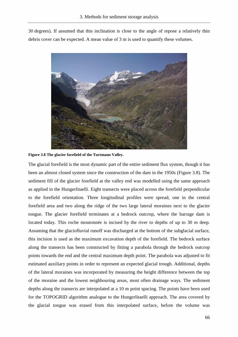
3. Methods for sediment storage analysis
66
30 degrees). If assumed that this inclination is close to the angle of repose a relatively thin
debris cover can be expected. A mean value of 3 m is used to quantify these volumes.
Figure 3.8 The glacier forefield of the Turtmann Valley.
The glacial forefield is the most dynamic part of the entire sediment flux system, though it has
been an almost closed system since the construction of the dam in the 1950s (Figure 3.8). The
sediment fill of the glacier forefield at the valley end was modelled using the same approach
as applied in the Hungerlitaelli. Eight transects were placed across the forefield perpendicular
to the forefield orientation. Three longitudinal profiles were spread, one in the central
forefield area and two along the ridge of the two large lateral moraines next to the glacier
tongue. The glacier forefield terminates at a bedrock outcrop, where the barrage dam is
located today. This roche moutonnée is incised by the river to depths of up to 30 m deep.
Assuming that the glaciofluvial runoff was discharged at the bottom of the subglacial surface,
this incision is used as the maximum excavation depth of the forefield. The bedrock surface
along the transects has been constructed by fitting a parabola through the bedrock outcrop
points towards the end and the central maximum depth point. The parabola was adjusted to fit
estimated auxiliary points in order to represent an expected glacial trough. Additional, depths
of the lateral moraines was incorporated by measuring the height difference between the top
of the moraine and the lowest neighbouring areas, most often drainage ways. The sediment
depths along the transects are interpolated at a 10 m point spacing. The points have been used
for the TOPOGRID algorithm analogue to the Hungerlitaelli approach. The area covered by
the glacial tongue was erased from this interpolated surface, before the volume was

3. Methods for sediment storage analysis
67
calculated. Thus, debris underneath the glacier is not considered here. Very few studies
quantified pro-glacial sediments (Small 1987; Etzelmüller 2000). These studies show large
differences in both methods and result and are difficult to compare the approach used her,
because no sediment thickness information is reported for pro-glacial debris.
3.4.3 Calculation of denudation rates and mass transfer
The denudation rate (DR) for the Turtmann Valley is calculated using equation 2.5. A mean
bedrock density ρb of 2.7 g cm-3 for the lithology of the Turtmann Valley (mica-shist, gneiss
and dolomite) is applied. Density of deposits depends on the consolidation process and the
state of the landforms and is assumed to be higher for glacial and fluvial deposits than for
talus or rock glacier deposits. Debris density values determined or applied in other studies
range from 1.5 to 2.6 g cm-3 (Jäckli 1957; Rapp 1960; Hinderer 2001; Sass and Wollny 2001).
As this study includes different types of storage landforms a mean value of 1.6 g cm-3 is
applied to calculate the DR. A time period of 10 ka was used for the DR calculation.
Denudation rates are calculated for the entire valley, the hanging valleys, the glacier forefield
and the Hungerlitaelli. For each part two denudation rates are determined, one based on the
total area, another based on the area of the current sediment sources, including bedrock
outcrops and glaciers. The total mass transfer per area represents the volume of material in
tons per area and time. Mass transfer is similar to sediment yield and calculated using
equation 2.2 for the same land surface parts of the valley. In contrast to the sediment yield, the
mass transfer relates to material that has not left the denudation area. The unit for mass
transfer per area is t km2 a-1.
Additionally, denudation rates for single landforms are calculated using equation 2.5. Four
landform types are used to derive single landform denudation rates: (1) talus slopes, (2) talus
cones, (3) block slopes, and (4) active rock glaciers. These landforms were chosen because
their source area can be defined with the greatest confidence. Sediment sources for talus
slopes, talus cones and active rock glaciers were determined by using the WATERSHED
command in ArcGIS 9.1. Taking the upper boundary of the landform as the source locations
the algorithm calculates the potential drainage area above the landform. This is assumed to
correspond to the source area of the debris that builds up the landform. Denudation rates of
block slopes are based on the entire block slope area.

3. Methods for sediment storage analysis
68
3.4.4 Uncertainties and error estimation of bedrock detection and volume
estimation
3.4.4.1 Uncertainties of bedrock detection using geophysical methods
Geophysical methods include inherent uncertainties due to the inverse problem (cf. chapter
3.4.1). Another source of uncertainty, especially in mountain terrain, results from similar
physical characteristics of frozen ground and bedrock that can lead to a biasing of the
interpretation (cf. chapter 3.4.1.1). However, with increasing application of these methods in
geomorphology, and hence more experience with the equipment and subsurface material,
uncertainties will decrease. Additionally, the combination of the different methods, as partly
performed in this study helps to explain uncertain or doubtful results (cf. Hoffmann and
Schrott 2003; Otto and Sass 2006), especially when other subsurface information from
boreholes, for example is missing.
Regarding the seismic refraction method, different inversion techniques have been applied
and combined in order to generate propagation velocities and bedrock surfaces. This can be
regarded as a cross check that the model used is realistic, or at least consistent with other
modelling results, which may also be wrong. Here, the network raytracing method provided
the most useful results, which were often, but not always, in good agreement with the
tomography inversion results (cf. chapter 5.2.1). Differences range from a few meters to more
than 10 meters. The network raytracing method itself provides a source of uncertainty when
the artificially calculated travel-times are fitted to the observed ones. This fit depends on the
quality of the recorded first-arrivals, which are never as symmetrical as the artificially
calculated travel-times. Thus, occasional outliers do occur for single rays. The modelling here
was stopped when a good overall fit for both types of travel-time was established. Further
modifications in order to eliminate single differences would have brought about changes in
the order of some 1-2 m of depth of the refractor surface.
The inversion of electric resistivity data strongly depends on the inversion algorithm used.
The algorithm used here (cf. chapter 3.4.1.2) is one of the most widely accepted and
frequently applied in geomorphology, and is therefore regarded as reliable. The inversion
software Res2Dinv enables the modification of a great variety of inversion parameters. These
include the size of the model blocks, damping parameters, a horizontal structure filter or a
factor of layer increase with depth. These parameters have been tested and the results
compared visually. The configuration used is assumed to suit to the expected subsurface
situation and detection of inclined, linear structures best. A complete list of the parameters

3. Methods for sediment storage analysis
69
used is attached in the appendix. The quality of the inversion is highest for a small number of
iterations and a small root mean square error (RMS). However, these values don’t ensure that
the modelled structures correspond to the reality. A sharp change in resistivity was often
detected at the regolith–bedrock boundary. However, a value range of 2-3 k Ω m, rather than
a single value, indicates the occurrence of bedrock. Thus, the bedrock boundary location
could only be determined within a depth range. This range is between 2 and 3 m.
Picking the exact location of the reflections is a potential source of error when analysing GPR
data. Another source of uncertainty is the applied radar wave velocity. The wave velocity
determined by WARR measurements is usually only valid for the upper few metres of the
material. Because the velocity influences the depth calculation, the location of deeper
reflections could be overestimated. However, no solution for this problem is discussed in the
literature. Sass (pers. communication 2006) estimated this error to be less than 15%. More
problematic is the correct interpretation of the reflections itself. Reflections in the radargram
are interpreted as bedrock, but in reality they are also caused by loss of wave energy. This
uncertainty can only be overcome by experience in radargram interpretation and no error
estimation is possible here. To conclude, the detection of the regolith–bedrock boundary by
geophysical surveying is assumed to include an average error of 5–10%.
3.4.4.2 Error estimation in volume calculation
The interpolation of sediment thickness in the Hungerlitaelli is based on field data and
estimated depth information. Field data are liable to the above discussed points of uncertainty.
However, the number of survey points is limited in relation to the size of the Hungerlitaelli
and the number of landforms observed. Estimations of interpolation points rely on
geomorphological analysis and interpretation of the observed land surface and are backed up
by a comparison with observations made in preceding studies in similar environments.
Corresponding to the position of the sediment storage landform in the hanging valley,
uncertainty about sediment storage depth varies. In general, sediment thickness of landforms
at lower locations, for example rock glaciers and moraine deposits, is assumed to be
underestimated, especially where estimation is based on the landform height above the
surface. In contrast, on talus and block slopes at upper elevations regolith depth might be
overestimated. Other studies on block slopes indicate very shallow regolith thickness of only
a few centimetres (Ballantyne and Harris 1994) compared to the 0.5-2 m assumed here. An

3. Methods for sediment storage analysis
70
uncertainty of 20–50% is assumed for the sediment thickness interpolation in the
Hungerlitaelli.
The transfer of regolith thickness information from the Hungerlitaelli to other hanging valleys
is based on the mean regolith depth of each landform type found in the Hungerlitaelli. An
application of mean depths for landform types naturally causes an error in the volume
calculation as variations both within single landforms and between landforms are eliminated.
Size, shape and position of the landforms within one type can differ widely and consequently,
volumes will be affected strongly by landform size and area–height ratio. This is especially
the case for moraine deposits, because lateral and basal moraines have been included in only
one class despite large differences in area–height ratio. Thus, the modelled sediment volumes
of the hanging valleys include a significant uncertainty with a degree of error of 50–100%.
Trough floor volume calculated by the SLBL approach depends on the assumption that the
morphology of the trough can be modelled with parabolas. As Hoffmann and Schrott (2002)
have shown this assumption leads to an overestimation of the trough volume, because the
bedrock surface is generally flatter then the parabola of a curve. The applied maximum
thickness relates to the few similar studies (Finckh and Frei 1991; Hoffmann and Schrott
2002; Schrott et al. 2003), though a valley the size of the Turtmann Valley has never been
studied before. The maximum depth of the valley floor is assumed to include an error of
20-50%. A constraint of the SLBL algorithm is the strong dependency of the modelled depth
on the valley width (cf. chapter 5.3.2.2). This creates shallower locations in narrow valley
floor parts. About 12% of the valley floor is less than 100 wide, while the average width is
about 180 m. At these narrow parts the modelled bedrock depth is significantly
underestimated compared to the wider parts. The overall error in trough volume is considered
to be 20-50%.
The volume calculation of the glacier forefield bases upon interpolation of estimated
parabolic transects. Several sources of uncertainty can be identified. First, the maximum depth
may be underestimated, as no information about over-deepend trough parts in the glacier
forefield is available, nor considered. Such over-deepening is possible at the former
confluence of the Turtmann and Brunegg glaciers and before or behind roche moutonées.
Another source of uncertainty is the depth of the two lateral moraines. The height of these
landforms is estimated relative to the neighbouring valley floor. However, no information
about buried bedrock or underlying glacial deposits is available and this could lead to an over-
or underestimation of the volume. To conclude, an error of 20-50% is considered here.

3. Methods for sediment storage analysis
71
The volume of the remaining areas is entirely based upon assumptions. No mean regolith
thickness for valley slopes or trough slopes could be found. Although, the mean depth values
applied in the modelling are considered to be rather conservative, an error of 50-100% is
possible.
To conclude, though the errors estimated for the single subsystems include a large
uncertainty, the errors include both over- and underestimations. Consequently, errors may
equalise as well as reinforce each other. In general, the sediment volume modelled is
considered rather a minimum scenario based on the geomorphological analysis in the field. A
proof of this assumption is only provided by further geophysical soundings in other hanging
valleys.
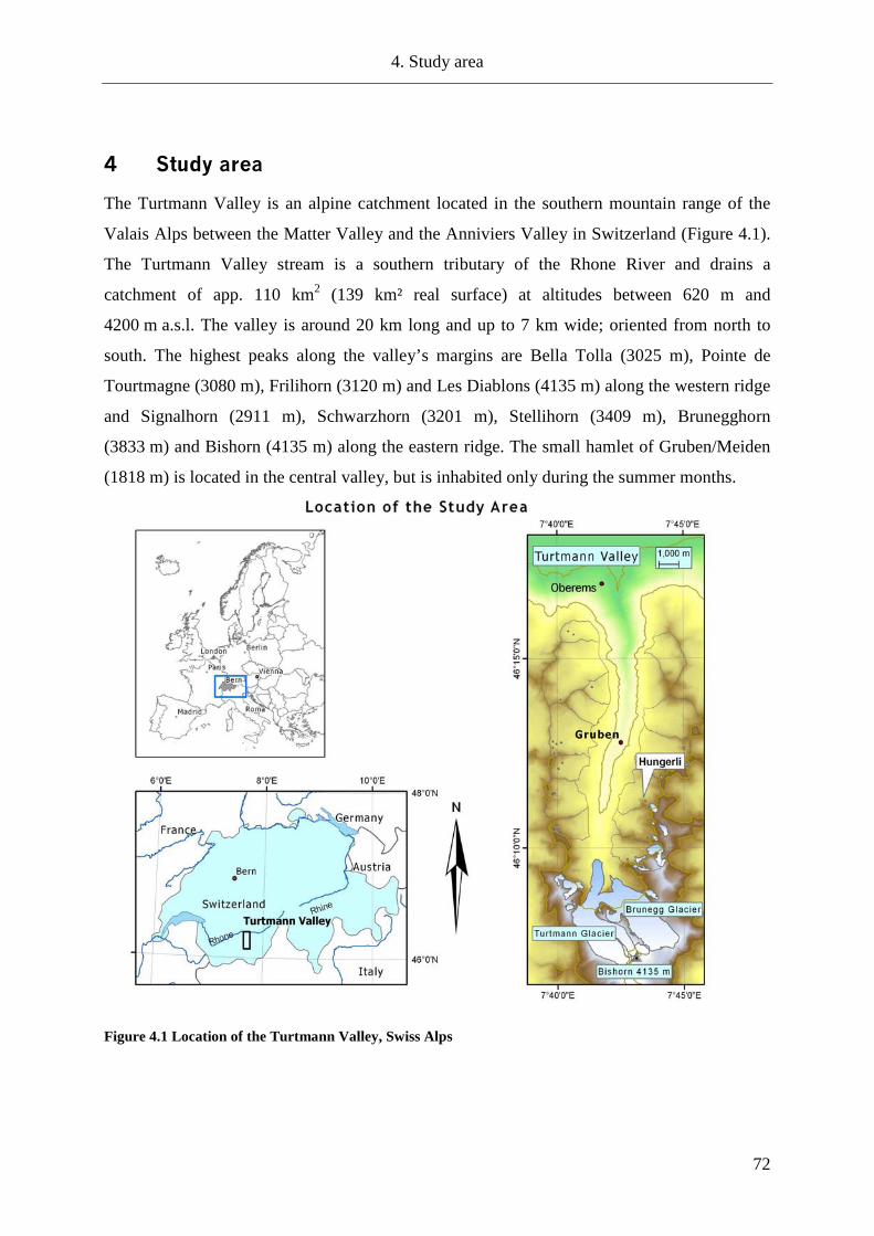
4. Study area
72
4 Study area
The Turtmann Valley is an alpine catchment located in the southern mountain range of the
Valais Alps between the Matter Valley and the Anniviers Valley in Switzerland (Figure 4.1).
The Turtmann Valley stream is a southern tributary of the Rhone River and drains a
catchment of app. 110 km2 (139 km² real surface) at altitudes between 620 m and
4200 m a.s.l. The valley is around 20 km long and up to 7 km wide; oriented from north to
south. The highest peaks along the valley’s margins are Bella Tolla (3025 m), Pointe de
Tourtmagne (3080 m), Frilihorn (3120 m) and Les Diablons (4135 m) along the western ridge
and Signalhorn (2911 m), Schwarzhorn (3201 m), Stellihorn (3409 m), Brunegghorn
(3833 m) and Bishorn (4135 m) along the eastern ridge. The small hamlet of Gruben/Meiden
(1818 m) is located in the central valley, but is inhabited only during the summer months.
Figure 4.1 Location of the Turtmann Valley, Swiss Alps

4. Study area
73
4.1 Geomorphology
The Turtmann Valley is a typical, glacially-shaped, high Alpine valley. The main valley can
be separated into two parts: The lower section of the Turtmann Valley is v-shaped covering
approximately one third of the valley's total length. It opens into an up to 300 m wide glacial
trough that terminates at the complex of Turtmann and Brunegg glaciers (Figure 4.2).
Fourteen hanging valleys (called Taelli in the local dialect) are located on both sides of the
trough slopes (Figure 4.3) most of them oriented west-east. Hanging valley floor elevation
increases from 2300 m to 2600 m from north to south. In addition to some of the hanging
valleys, which contain small glaciers, the dominant ice surfaces of the Turtmann and Brunegg
glaciers at the valley head cover about 14% of the valley surface. The hanging valleys contain
a typical set of high alpine processes and landforms with an observable strong influence of
periglacial processes. Rock glaciers are very frequent and almost every slope is modified by
small-scale periglacial creep. The main valley floor is characterised by a mixture of large
fluvial and debris-flow cones, avalanche tracks and glaciofluvial terraces. Areas below
2600 m on north facing slopes and 2800 m on south facing slopes show continuous vegetation
cover. Rock fall, rock glacier and solifluction creep and avalanches are the most active
processes, while debris flows only occur randomly along the main valley trough and around
the Turtmann glacier forefield. Most fluvial sediment transport is inhibited by the deviation of
the majority of the surface drainage from the hanging valleys into the barrage in the glacier
forefield. The main stream is almost completely disconnected from the glaciofluvial sediment
drainage system due to the construction of the barrage, since the water is entirely routed into
the neighbouring Anniviers Valley.

4. Study area
74
Figure 4.2 The southern end of the Turtmann Valley terminated by the Turtmann glacier to the right and Brunegg glacier to the left. The peaks in the left background are Bishorn (4135 m) and Weisshorn (4504 m)
Figure 4.3 View from the Hungerlitaelli across the main trough into some western hanging valleys. The peak towards the left is Les Diablons (3609 m).

4. Study area
75
4.2 Geology
The study area is located within the middle-penninic Bernard nappe that covers large areas of
the valaisanne Alps south of the Rhone valley (Labhart 2001). This nappe is divided into
several sub-units with the Siviez-Mischabel nappe (S-M) as the main part (Figure 4.4).
Lithostratigraphically the S-M nappe contains different methamorphic layers that consist
mainly of micashists and paragneisses. Palaeozoic shists and gneisses build up most of the
northern and eastern parts of the valley and dominate the lithologic setting (Bearth 1980).
Mesozoic dolomites, limestones and marbles in western and south-eastern parts of the
Turtmann Valley are easily distinguishable because they form large cliffs, like for example in
the Pipjitaelli. They cover the crystalline rocks and are wedged between the S-M nappe and
the overburden Dent Blanche nappe. The rocks of the S-M nappe are heavily folded and often
contain thin layers of amphibolites, quarzites and eclogites (Bearth 1980; Rahn 1991). The
general strike direction is south-west with average dipping between 20 to 30 degrees influence
by the folding of the nappes (Bearth 1980). The inclination of the bedrock influences the
formation of rock walls and slopes. Slopes inclining perpendicular to the bedding result in
steep rock walls and the formation of talus slopes and cones. In contrast, slopes dipping
parallel to the bedrock inclination favour the development of block slopes (Cruden and Hu
1996).
Figure 4.4 Geological cross section through the penninic nappes around the Turtmann Valley. The nappes are: 1–Houillère-Pontis, 2–Siviez-Mischabel, 3–Mont Fort, 4–Monte Rosa, 5–Zermatt-Sass Fee, 6– Tsaté, 7–Dent Blanche (from Laphart 2001)
4.3 Climate
The inner alpine location of the Turtmann Valley produces continental climatic conditions.
The valley is sheltered from heavy precipitation brought about by major frontal systems from
the southwest and southeast. Thus, comparably low precipitation and increased temperatures
characterise the entire southern Valaisan Alps. The climatic snow line is elevated under these
conditions as well, rising to an altitude of 3450 m (Escher 1970). Mean annual precipitation
ranges between 575 mm in Sion (482 m) and 710 mm in Visp (640 m) for lower stations
(Rhone Valley) higher stations (Zermatt, 1638 m & Evolène 1825 m) receive between 600

4. Study area
76
and 700 mm of precipitation per year. Mean annual air temperature varies between 8.5o C in
the Rhone valley at Sion and 3.5o C in Zermatt (Meteoschweiz). In 2002 climatic monitoring
started in the Hungerlitaelli. During the three year of recording, some probable climatic trends
can be observed. Temperature distribution thoughout the year shows a minimum in February
and a maximum in August (Figure 4.5).

77
Average daily temperature [°C] at 2 meters height a nd average daily precipitation [mm]
0
1
2
3
4
5
6
09.0
7.-3
1.07
.
01.0
8.-0
6.08
.
13.0
9.-3
0.09
.
Oct
ober
Nov
embe
r
Dez
embe
r
Janu
ary
Feb
ruar
y
Mar
ch
Apr
il
May
June
July
01.-
19.0
8.
07.1
1. -
30.
11.
Dec
embe
r
Janu
ary
Feb
ruar
y
Mar
ch
Apr
il
Mai
June
July
Aug
ust
Sep
tem
ber
Oct
ober
Nov
embe
r
Dec
embe
r
Janu
ary
Feb
ruar
y
Mar
ch
Apr
il
May
June
July
Aug
ust
01.0
9. -
23.
09.
2002 2003 2004 2005
Time
mm
-15
-10
-5
0
5
10
15
°C
Precipitation
Temperature
Figure 4.5 Mean annual air temperature and monthly precipitation figure from the climate station in the Hungerlitaelli (Altitude 2770 m).

4. Study area
78
The Mean annual air temperature is -1.2o at an altitude of 2770 m a.s.l. indicating that the
lower limit of permafrost lies around this altitude (Nyenhuis 2005). Precipitation is highest in
August. However, snow is not registered and therefore not included in this record. Between
September 2004 and August 2005 492.6 mm of rain have been measured. About 20% of this
precipitation (92 mm) was recorded in August 2005. Summer precipitation often occurs as
thunderstorms that develop in the late afternoon and can bring significant amounts of rain.
Especially the southern part of the Turtmann Valley is often affected by thunderstorms that
form around the largest peaks. Debris flows around the glacier forefield have been observed
caused by such events.
4.4 Glacial history and paleoclimate
The Swiss Alps are among the best studied regions of quaternary glaciation. The introduction
of a general theory on glaciation, established in the 18th and early 19th century by Agassiz and
predecessors, marks the onset of glacial research. The famous works by Penck and Brückner
(1909) lead to a differentiation of distinct phases of quaternary glacial retreat at the end of the
Würm glaciation in the Alps. Their classical division into the three main stages “Bühl –
Gschnitz – Daun” has since been verified and refined by various authors. Eight major stages
of glacial extends have been classified based on moraine mapping for the Alps (Maisch 1982).
The lowest extend (Bühl) is located around 1000 m below the Little Ice Age (LIA) reference
level.
The Late-Glacial maximum glacier extend during the last glaciation (Würm) in the western
Swiss Alps was studied by Kelly et al. (2004a) Based on mapped trimlines and other
evidences of glacial erosion on bedrock, they concluded that the ice surface reached altitudes
up to 2600 m in the Rhone valley near Brig, dropping to 1600 m towards Lake Geneva. For
the Turtmann Valley only rough interpolated information is given, indicating for the main
valley floor an ice surface altitude between 2200 and 2800 m, rising towards the hanging
valley cirques and the Bishorn peak (4058 m). Thus, most of the peaks in the Turtmann
Valley would have been free nunataks.
A detailed mapping of the moraines has been done by Otto (2001) and Wolff (2006).
However, no dating of moraine deposits and glacier extents exists. Wolff (2006) associates
mapped moraine locations in the Turtmann Valley with comparable studies from
neighbouring locations in the Valais. Detailed glacier histories of neighbouring areas have
been accomplished by Bircher (1983) for the Sass Valley, Müller (1984) for the Simplon area
and Val de Nendaz, and by Haas (1978) for the Zinal Valley.

4. Study area
79
The Egesen stage marks the most wide-spread, prominent extend towards the end of the late
glacial. Egesen moraines are often well preserved and because of their larger size compared to
the LIA moraines frequently observed throughout the Alps. Maisch (1982) locates the Egesen
stage between 170 and 240 m below the 1850 snow-line level. The mean 1850 snow-line
altitude for the study area is around 2906 m (mean value for the Dent Blanche glacier region,
after Maisch et al. (1999). Hence, a paleo-snow-line for the Egesen stage in the Turtmann
Valley would have been located between 2660 and 2730 m. In comparison, the 1973 snow-
line has been determined at around 3200 m for the study area (National Snow and Ice Data
Centre 1999). The main valley floor does not show remains of distinct moraine deposits
below the 1850 extend, or near the inferred Egesen level. However, in some of the hanging
valleys large lateral and frontal moraines can be observed. Although no dating information
exists on these moraines, they can be associated with Daun and Egesen levels based on snow-
line modelling Wolff (2006).
The Egesen stage is associated with the Younger Dryas time period. This period represents a
late glacial climate depression at end of the Pleistocene glaciation and is usually dated
between 11,000 and 9,500 BP. In the neighbouring Saas Valley, Bircher (1982), using 14C and
pollen records dated bog sediments associated with the Egesen stage at 1800 m a.s.l. to
9760 ±175 yr BP. Transferring this altitude level to the Turtmann valley, the Younger Dryas
extent of the Turtmann glacier complex would have been located near the settlement of
Gruben. A map created by Burri (cited in: Schweizerische Gesellschaft für Ur-
undFrühgeschichte 1993) showing the Younger Dryas glacier extent in the Valais supports
this assumption (Figure 4.6). Kelly et al. (2004b) dated the Egesen moraine of the Great
Aletsch glacier to 9640 ±430 yr BC using cosmogenic nuclide 10BE. However, this glacier is
not comparable to the Turtmann Valley glaciers due to its larger size.

4. Study area
80
Figure 4.6 Younger Dryas extent in the Valais, Switzerland. (modified after Burri 1990, from: Schweizerische Gesellschaft für Ur- und Frühgeschichte 1993)
The Holocene glacier and climate fluctuations have been investigated in numerous studies
through out the Swiss Alps. Methods applied include lake sediment analysis (varves, pollen,
and others, e.g. Leemann and Niessen 1994; Haas et al. 1998; Heiri et al. 2003), 14C dating of
fossil soils and woods (Röthlisberger 1976; Hormes et al. 2001; Holzhauser et al. 2005),
dendrochronology (Holzhauser and Zumbühl 1996), lake level variation analysis (Holzhauser
et al. 2005) and more recently surface exposure dating (Ivy-Ochs et al. 1996; Kelly et al.
2004b). Studies on lake sediments, using varve analysis of proglacial lake sediments at lake
Silvaplana, Eastern Switzerland, determined the end of the Younger Dryas at 9400 BP
(Leemann and Niessen 1994). Additionally, the study by Leemann and Niessen (1994)
observes that there wa sonly minor glacial acitivty in this catchment from 9400-3300 BP.
Most recent glacier fluctuations since the Little Ice Age (LIA) are recorded only for the
Turtmann glacier. Reliable information on most Late Holocene glacier extents in the hanging
valleys is very scarce. However, some information about the LIA maximum extent of some of
the smaller glaciers does exists (Maisch et al. 1999).

4. Study area
81
4.5 Previous work in the Turtmann Valley
Previous research in the Turtmann Valley focused on glacial and periglacial geomorphology
as well as geomorphometry. Rock glaciers have first been studied by van Tatenhove and
Dikau (1990) using geophysical methods. This work was continued by Pfeffer (2000), von
Elverfeld (2001), Nyenhuis (2005) and Roer (2005), working on permafrost distribution
(Pfeffer, Nyenhuis) and rock glacier kinematics (von Elverfeld, Roer). Glacial research
include the study of push moraines in the Turtmann glacier forefield (Eybergen 1986) and the
observation of drumlin in the Augsttaelli (van der Meer and van Tatenhove 1992). Most
recently, the barrage in the glacier forefield has been investigated by hydrological engineers,
as the volume of the barrage is almost filled up with sediment. Technical modifications to the
forefield have been studied in order to prevent further silting-up and keep the barrage
functioning (Martinerie et al. 2005). The Late Glacial and Holocene moraine distribution has
been studied by Wolff (2006), who models paleo snow-line altitudes based on his field
mapping.
A geomorphological map was compiled by Otto (2001) that was used to construct a first
qualitative sediment flux model of the valley (Otto and Dikau 2004). The first study on
sediment storage was carried out by Knopp (2001).
Rasemann (2004) analysed the geomorphometric structure of the land surface using DTM
data in GIS. A semantic modelling of geomorphological landforms based on the sediment
cascade principle was performed by Löwner (2005). König (2006) used remote sensing
methods on the HRSC data to derive grain-size distribution from sediment storage landform.
The distribution of vegetation was studied using remote sensing techniques by Hörsch (2003).

5. Results
82
5 Results
5.1 Characteristics and spatial distribution of sediment storage landforms
A total of 593 sediment storage landforms have been mapped in the fourteen hanging valleys
of the Turtmann Valley in an area of around 58 km2 (Figure 5.1). About 75% of this area is
covered by sediment; the remaining parts of the surface include bedrock, glaciers and lakes.
Sediment is trapped in lakes and underneath glaciers, however these deposits will not be
considered here. More than 50% of the land surface covered by sediment is classified as slope
deposits that include talus slopes (20%), talus cones (2.5%) and block slopes (28.7%).
Moraine deposits cover around 37% of the land surface, followed by 11% covered by rock
glaciers and 2% by alluvial sediments and rock fall deposits (Table 5.1). Mean landform size
ranges from around 10,000 m2 for alluvial deposits and protalus rock glaciers to more than
175,000 m2 for moraine deposits, covering entire hanging valley floors. Slope storage
landforms, talus slopes, talus cones and block slopes cover 42,000 m2, 35,000 m2 and 85,000
m2 respectively. Rock glaciers have average sizes of 67,000 m2 for active forms, 23,000 m2
for inactive ones and 72,000 m2 for relict rock glaciers.
Table 5.1 Sediment storage size and altitudinal distribution
Sediment storage landform type
Number of objects
Proportion of land surface (%)
Area (106 m2)
Mean area (m 2)
Min. altitude (m)
Max. altitude (m)
Talus slope 191 14.2 8.1 42,250 2264 3328 Talus cone 29 1.8 1.0 35,329 2199 3171 Block slope 143 21.5 12.2 85,485 2150 3261 Moraine deposit 89 27.4 15.6 175,075 2137 3227 Rock fall deposit 24 0.4 0.3 10,442 2406 2936 Alluvium 24 1.0 0.6 24,221 2152 2791 Rock glacier (active) 36 4.2 2.4 67,113 2419 2968 Rock glacier (inactive) 24 2.0 1.1 26,717 2426 2727 Rock glacier (relict) 22 2.3 1.3 74,168 2237 2760 Rock glacier (protalus) 9 0.2 0.1 11,811 2442 2789
Total landform cover 593 74.7 42.5 Other: Bedrock - - 13.2 Glacier - - 1.1 Lakes - - 0.1
Total Area - 100 57.0

5. Results
83
Figure 5.1 Land surface classification of the hanging valleys

5. Results
84
The hanging valleys are located at altitudes between 2137 and 3589 m a.s.l. The highest
accumulation of sediment is found at 3328 m. Figure 5.2A depicts the altitudinal distribution
of the land surface area covered by the different storage landform types. Though influenced
by the hypsometric distribution of the hanging valleys (Figure 5.2B), the distribution reveals a
dominance of slope storage landforms in the upper locations (above 2700 m) in contrast to
lower altitudes that are primarily covered by glacial and alluvial deposits. The location of rock
glaciers shows a distinct correlation between altitude and state of activity, as active types are
found above inactive and relict types. Rock fall deposits are found between 2400 and 2800 m,
which indicates their position between slope foots and valley floors.
Figure 5.2 A - Altitudinal distribution of classifi ed storage land surface. B – Hypsometric curve of the hanging valley area.

5. Results
85
Mean geomorphometric parameters are given in Table 5.2. Slope inclination distribution
allows for a distinction of landform types with steeper inclination of slope types (28-31o) and
more gently inclined landforms like moraines and rock glaciers (19-23o); the lowest
inclinations are observed for alluvial deposits (10o). The aspect of the different landforms
shows little variation when considering average values (Table 5.2). However, a more detailed
distribution pattern is observed in a directional histogram for the single landforms. Figure 5.3
depicts the frequency distribution of mean aspect values for the single landforms classified
into the 8 major directions. The superimposed signal of the general hanging valley orientation
influences the data distribution as indicated by the two largest sectors facing ESE and WNW.
Looking at the proportional distribution within the direction classes some trends are
observable: Talus slopes dominate at northern directions as well as towards ESE. Block
slopes in contrast are generally facing towards southern directions. Moraine deposits follow
the general hanging valley orientations of ESE and WNW corresponding to their overall
position in the central and lower parts of the hanging valleys. Active rock glaciers have a peak
WNW, while rock fall and alluvial deposits do not reveal an orientation trend. Curvature is
not a good indicator for feature characteristics at this scale. Mean values of the almost 600
landforms don’t indicate any tendency for each of the curvature types. This is probably due to
a large scatter of values that is averaged out by observing mean values only.
Table 5.2 Geomorphometric parameters of storage landforms.
Sediment storage landform type
Mean slope (degrees)
Mean aspect (degrees)
Profile curvature (m-1)
Tangential curvature (m-1)
Max. curvature (m-1)
Min. curvature (m-1)
Mean curvature (m-1)
Talus slope 31 157 -0.0018 -0.0015 0.014 -0.018 -0.0017 Talus cone 28 171 -0.0013 -0.0007 0.013 -0.015 -0.0010 Block slope 31 182 -0.0003 -0.0003 0.016 -0.016 -0.0003 Moraine deposit 21 185 -0.0008 0.0001 0.018 -0.019 -0.0003 Rock fall deposit 21 163 -0.0027 -0.0015 0.021 -0.025 -0.0021 Alluvium 10 152 -0.0042 -0.0037 0.012 -0.020 -0.0040 Rock glacier (active) 21 210 -0.0001 0.0001 0.021 -0.021 0.0000 Rock glacier (inactive) 23 202 -0.0003 0.0006 0.022 -0.022 0.0001 Rock glacier (relict) 19 168 -0.0002 0.0001 0.023 -0.023 0.0000 Rock glacier (protalus) 22 194 -0.0006 -0.0008 0.021 -0.022 -0.0007

5. Results
86
Figure 5.3 Directional frequency distribution of mean aspect values for sediment storage landforms. (Colours correspond to Figure 5.2)
The analysis of secondary landform attributes (cf. chapter 3.2) focuses on the relative position
of the landforms with respect to drainage divides and drainage ways, as well as the relative
position of the landforms towards each other. The latter is expressed by the identification of
toposequences. Table 5.3 shows minimum and maximum distances of storage landforms to
the ridge and the drainage ways in the hanging valley. Distances have been calculated on a
pixel basis and are given in metres. The spatial arrangement observed in these distances fits
well to the landform types and their formative process behaviour. Block slopes do not have
overhanging rock walls, hence they start at the ridges, while talus slope are located in a
relatively small distance from the ridge separated by the rock wall. Rock glaciers are located
relative to the drainage divide with increasing distance according to their status of activity.
Moraine deposits cover areas within the largest maximum distance, including points at the
hanging valley entries, while alluvial deposits are located at the largest minimum distance to
the ridge. The position of the landforms types towards the drainage way is almost vice-versa.
Glacial and alluvial deposits flank the creeks. Rock fall deposits, relict rock glaciers and talus

5. Results
87
cones are located closest to the drainage ways, while active rock glaciers and block slopes
cover the most distant locations (according to the minimum distance).
Table 5.3 Mean minimum and maximum distance of storage landforms to ridges and drainage ways.
Min. distance to ridge
Max. distance to ridge
Min. distance to drainage way
Max. distance to drainage way
Sediment storage landform type
(m) (m) (m) (m) Talus Slope 35 1187 177 1806 Talus Cone 153 800 70 1733 Block Slope 0 1116 246 1994 Moraine Deposit 203 1654 0 2138 Rock fall deposit 295 999 113 1046 Alluvium 463 1301 0 639 Rock glacier (active) 73 1075 279 1764 Rock glacier (inactive) 133 675 288 1451 Rock glacier (relict) 192 1075 94 1605 Rock glacier (protalus) 97 709 118 1786
Seven toposequence types have been identified in the Turtmann Valley (Table 5.4) that
illustrate the topographic, downslope neighbourhood of the storage landforms. The most
frequent neighbourhood situation is toposequence type I: a talus slope or cone is located
bellow a rock face and adjacent to the moraine valley fill, followed by alluvium parts at lower
locations. Due to the high number of rock glaciers in the Turtmann Valley, their role in the
toposequence distribution is quite strong; about 39% of the toposequences and 4 out of 7
types (II, III, IV, and V) include rock glaciers. Here, talus derived rock glaciers dominate with
28% compared to 11% moraine derived forms. Figure 5.4 depicts toposequences of the types
I, II and VI in the Grüobtaelli hanging valley. In order to relate the toposequence approach to
a functional relationship between adjacent landforms, the sediment flux needs to be
considered (Table 5.4). Sediment flow directions and coupling of processes can be derived
from the spatial landform distribution. With respect to the coarse sediment flow, the current
transport cascade in the hanging valleys is very short, including a direct combination of
primary source areas (bedrock, moraine deposits) and first and second order storage
landforms. First order storage is the accumulation of material in closest proximity to the
primary source area. In case of toposequence I this is the talus slope that takes up the rock fall
debris. When sediment is transferred from this storage landform into another, for example by
periglacial creep, the second storage landform in the cascade is formed. For example in
toposequence type II, a rock glacier develops underneath a talus slope incorporating its debris.
Most of the storage landforms in the sediment cascades are decoupled from the adjacent
landform in the toposequence, caused for example by the absence of a process that removes
coarse debris from landforms like rock glaciers or talus slopes. Debris flow activity is very

5. Results
88
low and rock glacier creep usually simply overrides moraine deposits without adding to their
storage volume. With respect to fine sediment, fluvial outwash processes and debris flows
remove material and extend the sediment cascade into the main valley subsystem.
Table 5.4 Landform toposequence mapped in the Turtmann valley. The gray shaded sequence parts represent a landform coupling in a coarse debris sediment cascade.
I II III IV V VI VII
Rock face Rock face Rock face Block slope Glacier Block slope Rock face Talus slope/cone
Talus slope/cone
Talus slope/cone
Rock glacier Moraine Deposit
Moraine deposit
(Talus slope)
Moraine deposit
Rock-glacier
Rock glacier (active)
Moraine deposit
Rock-glacier
(Alluvium) Rock fall deposit
(Alluvium) Moraine deposit
Rock glacier (inactive)
(Alluvium) (Rock-glacier)
Moraine deposit
(Alluvium) (Rock glacier (relict))
Moraine deposit
(Alluvium)
Moraine deposit
(Alluvium)
(Alluvium) Frequency: 45 % 20 % 2 % 6 % 11 % 9 % 7 %
Figure 5.4 Different toposequences found in the Grüobtaelli. The roman numbers indicate the toposequence type (cf. Table 5.4)
5.1.1 Landform distribution within hanging valleys
Of the fourteen hanging valleys have been investigated in the Turtmann Valley eight are
located on the western side of the trough, and six are located in the east. The position of the
central valley axis strikes perpendicular to the main valley longitudinal axis in east-west
directions. Only the most northern hanging valleys differ from this orientation pattern towards

5. Results
89
north and south (Table 5.5). Mean valley size is 4 x 10⁶ m2, ranging between 1.7 x 10⁶ m2
(Simmigtaelli) and 8.3 x 10⁶ m2 (Bortertaelli). The hanging valley altitude increases towards
the south, following the general altitudinal trend from 2137 m in the Griebeltaelli to highest
elevations (3589 m) attained in the Pipjitaelli. The mean altitudinal range between the
hanging valley entry and the ridge is about 850 m. The relative storage area averages about
75%; the exception from this distribution is the the Pipjitaelli with only 47% of the land
surface covered by debris. This is influenced by a significant change in lithology that creates
higher and steeper rock walls compared to the other hanging valleys, adding to the
3-dimensional area.
Table 5.5 Geometric characteristics of the hanging valleys in the Turtmann Valley
Hanging Valley
3D-Area
Altitude (m) Orientation of central valley axis
Storage Area (%)
(106 m2) Min Max Augst 2.45 2365 3085 E 79.7 Blüomatt 4.00 2306 3079 E 78.6 Borter 8.27 2150 3025 NE 68.6 Brändji 4.32 2345 3396 W 58.4 Chummetji 3.46 2259 3029 NW 90.2 Frili 2.48 2384 3141 E 72.5 Griebel 2.03 2137 2873 NE 86.7 Grüob 6.03 2238 3169 W 79.7 Hungerli 4.22 2298 3273 W 77.5 Meid 5.35 2216 3084 E 78.2 Niggeling 5.24 2154 3204 W 81.8 Pipji 4.99 2431 3589 W 46.6 Rotig 2.46 2252 2960 SE 84.7 Simmig 1.67 2223 2849 SE 76 Total 56.95

5. Results
90
Figure 5.5 Relative landform storage type area (%) per hanging valley.
The internal distribution of storage types in the hanging valleys is depicted by Figure 5.5. At
first sight, each hanging valley seems to have its own composition of storage landforms.
Though the distribution appears very heterogeneous, the variations between the three main
and ubiquitous landform types, talus slopes, block slopes and moraine deposits are relatively
small, within some exceptions. Talus slopes most often cover between 15% and 25% of the
land surface. Larger relative areas are observed in Blüomatt- and Augsttaelli, while very few
parts are covered by talus slope debris in the Chummetjitaelli (8%). The latter is clearly
balanced by a dominance of block slopes here (50%). The block slope proportion ranges at an
average between 20% and 30%, the smallest relative coverage being found in the Meidtaelli
(17%). Moraine deposits cover at average between 35% and 45% of the hanging valley areas.
The large and especially wide Meidtaelli stands out here, with 55% of the surface being
covered with glacial sediments. The relative distribution of the remaining landform types
shows very little patterns. However, the rock glacier distribution reveals a culmination of
active rock glaciers in the hanging valleys to the east (Niggeling, Pipji, Hungerli, Grüob,
Brändji). In the Hungerlitaelli block slopes and moraine deposits are almost equally
distributed covering 30% of the land surface each. Rock glaciers contribute about 20%, while
talus slopes and cones cover about 15% of the valley. Protalus rock glaciers and alluvial
deposits are not observed in the Hungerlitaelli.

5. Results
91
5.2 Geophysical surveys
5.2.1 Detection of the regolith-bedrock boundary with seismic refraction
surveying (SR)
Refraction seismic soundings have been performed along 27 profiles in the Hungerlitaelli.
Profiles have been placed on talus slopes, talus cones, rock glaciers, moraines and along
central positions within the hanging valley (Figure 5.6). Most profiles spread parallel to the
slope inclination; but some perpendicular profiles have been added. Applying a geophone
spacing of 3, 4, and 5 m spreads of 69, 92 and 120 m respectively could be covered.
Subsurface structures have been detected at a maximum depth of 27 m. Table 5.6 gives a
summary of all seismic profiles. A detailed collection of all seismic modelling results can be
found in Appendix A.
All seismic records show an internal composition of two to three different subsurface layers.
Surface velocities of most of the spreads in an upper zone between 0.5 and 10 m thick are
between 200 and 800 m s-1. An intermediate layer of increased velocity follows in some of the
soundings, represented by velocities between 650 and 2000 m s-1. This zone is located at
depths from 2 to more than 30 m. 23 soundings show subsurface conditions that create wave
velocities of more than 2900 m s-1. Seventeen of them reveal a refractor layer that was
interpreted as bedrock with velocities 2900 and 4000 m s-1. The overburden layers above the
bedrock are interpreted as loose debris at the surface (200–800 m s-1) and compacted debris
within the landform (700–2000 m s-1). Higher velocities in regolith and associated compaction
can be due to different grain compositions, water and/or ice contents and hence may indicate
different accumulative times or processes. Infiltration of fines through large pores at the
surface leads to a reduction of pore space in deeper layers (van Stein et al. 2002) that can also
cause higher velocities. However, buried moraine deposits may be occurring within talus
slope as well, representing the action of different processes in the formation of a landform.
Permafrost has been observed in ten surveys, provoking wave speeds between 3500 and 4500
m s-1.
Permafrost is clearly observable in active rock glaciers (SR04_5r/l, SR05_6, SR05_8,
SR05_13), which hinders the distinction of the deeper bedrock layer. Thus, no sediment
thickness information could be derived for rock glaciers. At the foot of one talus slope
(SR05_1) a large permafrost area is observed, hence, here the dipping bedrock surface cannot

5. Results
92
be detected throughout the entire profile. In some cases geophysical surveys proved the
permafrost occurrence (compare for example SR05_1 and ER05_1). At two locations no
distinct layering can be observed. These profiles are both placed on glacial sediments. Spread
SR04_4 is located on the lateral margin of a rock glacier draining a small cirque. This margin
is interpreted, based on the sedimentological composition, as a lateral moraine merged with
the rock glacier side. Wave velocity of this material increases gradually downwards after a
shallow surface layer (mean depth 2.8 m) of 320–700 m s-1. Profile SR05_3 is a combination
of two overlapping spreads along the thalweg in the glacier forefield. The surface sediment
cover is composed of large clasts (size of 0.5–2 m), under which the sound of running water
could be heard from inside the slope. The modelled results reveal similar subsurface
characteristics in the two profile parts with increasing velocities downwards. However, the
lower part (left) of the profile shows an increase of velocity towards the surface in the central
part. This could probably be due to a large boulder buried in the debris that accelerates the
wave speed.
Figure 5.6 Location of seismic profiles (SR) and sediment storage landforms in the Hungerlitaelli. (For a description of landform colours please refer to Figure 5.1).

5. Results
93
Figure 5.7 depicts the modelling results of survey SR04_2. This survey will be discussed here
in more detail in order to exemplify the interpretation of the seismic modelling results. Survey
SR04_2 was placed on a small talus slope below the Hungerlihorli peak at an altitude between
2572 and 2624 m. The uppermost geophone was located about 1 m beneath the bedrock face.
The geophones were spaced 3 m apart generating a profile of 69 m in length. Shots were
triggered between every second geophone at a distance of 6 m. Two shots have been placed
before and after the spread at -7.5, -1.5, 70.5 and 75.6 m. The travel-times geometry indicates
a two-layer composition of the underground. A first layer is characterised by a wave velocity
of 350 m s-1 and dips parallel to the surface with depths increasing from 2.2 to 6 m. The
surface of the second refractor has more irregular profile (Figure 5.7C). A sharp drop of 5 m
at a distance of 20 m to the cliff interrupts a first surface parallel part close to the rock face at
a depth of 2–4 m. Below this drop the refractor surface has a slight curved shape dipping at
depth between 10 m in proximity to the drop and 6 m towards the end of the profile. The
modelled travel-times by the network raytracing method correspond quite well to the
observed ones, except for one shot in the centre of the spread (cf. Figure 5.7B), where the
observed travel-times show some irregularities. This could be caused by wrong picking of the
first arrivals. A comparison between the network raytracing and the tomography model shows
a comparably good representation of the shape of the lower refractor, including the sharp
drop, but slightly lower wave velocities in the tomography model. However, no indication for
the upper refractor is observable from the tomography results. Thus, the location of the
refractor surface is confirmed by two interpretation methods and can be regarded relatively
accurate.
According to the wave velocities of these three layers the internal composition of this slope is
interpreted as a regolith cover with increasing compaction and density downwards (velocities
350 to 800 m s-1) on top of a (possibly strongly weathered and fractured) bedrock surface with
a velocity of 2900 m s-1. The observed bedrock step in proximity to the rock face may indicate
a buried rock face or step.
The propagation velocities of waves in debris and bedrock material observed in this study
correspond well to values given in general textbooks (cf. Chapter 3.3) and preceding studies
in the Turtmann valley by Pfeffer (2000), Knopp (2001) and Nyenhuis (2005). Pfeffer (2000)
and Knopp (2001) reported p-wave velocities between 100 and 2000 m s-1 for loose debris,
between 1700 and 4000 m s-1 for frozen ground and 2600–4000 m s-1 for bedrock. Nyenhuis
(2005) looking for Permafrost in the upper Hungerlitaelli stated wave velocities between 300

5. Results
94
and 1900 m s-1 for unfrozen debris and values of 2700–3800 for permafrost locations.
However, Nyenhuis (2005) never reached bedrock in his study.
Maximum regolith thickness derived from seismic refraction soundings in the Hungerlitaelli
for talus landforms range from 18 m on block slopes to more than 30 m on talus cone.
Moraine deposits show a sediment thickness of more than 33 m in the central part of the
Hungerlitaelli on former basal moraine deposits and of more than 16 m on a lateral moraine at
the valley entry. Knopp (2001) gives similar values for the neighbouring Braendjitaelli
towards the south. He observed the bedrock surface underneath talus cones at 20 to more than
36 m, while for glacial deposits he gives thickness values between 5 and 28 m. Rock glaciers
in his study have been estimated to be at least 13-24 m thick. For alluvial deposits in the
valley bottom Knopp (2001) observed sediment thickness between 2 and 11 m.

95
Table 5.6 P-wave velocities and refractor depths of seismic profiles in the Hungerlitaelli.

5. Results
96
Figure 5.7 Sounding SR04_2: Model of refractor locations and velocity distribution (A), travel-times (B) and cross-section of refractor layers (C). The seismic modelling includes the location of the refractor surfaces calculated with the network raytracing method and of the velocity distribution derived from the tomography modelling. The numbers give the velocities (in m s-1) of the modelled layers using the network raytracing method. Diagram B shows the observed (black lines) and modelled (coloured lines) travel-times of this sounding. The colour scale on the right refers to the modelled velocity distribution derived from the tomography modelling. The lower diagram (C) depicts a cross-section through the talus slope indicating the location of the two observed refractor surfaces.

5. Results
97
5.2.2 Detection of the regolith-bedrock boundary using Electric Resistivity
Tomography (2D-ER)
Fifteen, two-dimensional electric resistivity soundings (2D-ER) were conducted in the
Hungerlitaelli (Figure 5.8). On talus slopes, talus cones and block slopes profiles were spread
parallel and, at two locations, perpendicular to the slope inclination. In central positions of the
hanging valley, the profiles followed the line of steepest inclination and lowest elevation
(thalweg). Profile lengths were 120, 160 and 200 m with electrode spacing of 2, 3 and 4 m,
respectively. The penetration depth of the electrical current in the subsurface was between 12
to 30 m with a mean depth of 22 metres. Table 5.7 gives a summary of the 2D-ER
measurements. The graphics of the modelled resistivities along all profiles can be found in
Appendix B.
Figure 5.8 Location of the electric resistivity profile (2D-ER) and sediment storage landforms in the Hungerlitaelli. (For a description of landform colours please refer to Figure 5.1).

5. Results
98
Resistivities generally ranged between < 3 k Ω m and 50 k Ω m. Only two profiles, ER05_1
and ER05_4, show values above 100 k Ω m. These high resistivities can be caused by a local
occurrence of permafrost or due to very dry conditions. At profile ER05_1 resistivities
increased with depth at the lower end of the profile from below 10 k Ω m to values above
100 k Ω m. This slope is located in the recently deglaciated forefield of the Rothorn glacier,
and high resistivity at this location is interpreted as permafrost, possibly the remains from a
frozen lateral moraine now buried by talus deposit. The profile ER05_4 was a critical survey
with strong contact difficulties between the electrodes and the rocks. Therefore, very few data
points entered the inversion modelling produced a high RMS error of more than 25%.
Permafrost is unlikely in this situation (south facing slope at 2700 m altitude) and these high
values are possibly due to very dry debris with large, air-filled pores. One profile, ER05_4,
showed values below 5 k Ω m over most of the spread. The location of this profile in the
thalweg of the glacier forefield coincides with the main drainage way of the glacier’s
meltwaters. These waters seep into the coarse debris some 50 m above this location and
percolate downhill below the surface, which can be observed acoustically at few locations.
This subsurface drainage may be responsible for the low resistivities along the profile, even
though the surficial rock cover appears to be dry.
Table 5.7 2D-ER soundings in the Hungerlitaelli.
Length: Spacing: Max. depth: Boundary observable by strong resistivity contrast
Boundary interpreted as:
Profile name:
(m) (m) (m) (yes/no) ER04_1 200 5 26 yes Permafrost ER04_1q 160 4 21 yes ambiguous ER04_2 160 4 24 no -- ER04_3 80 2 12 yes Bedrock ER04_4 160 4 15 yes Bedrock ER04_5 200 5 30 yes Bedrock ER04_5q 160 4 18 yes Bedrock ER04_5q2 160 4 19 yes Bedrock ER04_6 120 3 18 yes Bedrock ER05_1 120 3 18 yes Permafrost ER05_2 160 4 24 no -- ER05_3 200 5 30 no -- ER05_4 160 4 25 yes Bedrock ER05_5 160 4 24 no -- ER05_6 200 5 30 yes ambiguous
In order to acquire the apparent resistivity for the underlying bedrock in the study area some
profiles were located in immediate proximity to surficial bedrock like rock walls or outcrops.
Figure 5.9 shows profiles ER04_5q and ER04_5q2 in a combined inversion. The two
soundings overlap in the central part by 60 m. The eastern (right) part of the profile passes a

5. Results
99
rock wall at a distance of app. 2 m. Thus, the sharp resistivity drop from 20 k Ω m to less than
7.5 k Ω m at a depth of app. 3.5 to 5 m below the surface is interpreted as the bedrock surface.
The same feature is apparent on the western (left) half of the profile at a depth of 13 m. This
boundary can be detected at the perpendicular profile ER04_5 and is observable in the
corresponding SR soundings (RS04_1 and RS04_3) as well. The boundary observed here is
interpreted as the regolith- bedrock boundary with a resistivity value between 5 k and 7.5 k Ω.
In earlier electrical survey studies on comparable landforms in the Turtmann valley, Nyenhuis
(2005), studying the permafrost distribution in the source area of a rock glacier near the
Rothorn glacier (upper Hungerli hanging valley), apparently never reaches the bedrock. His
measurements reveal resitivities above this threshold. Pfeffer (2000) and Knopp (2001) also
measured resistivity in the southern adjacent hanging valley of the Hungerlitälli the
Brändjitälli. They considered resistivity values between 2 and 10 k Ω m representative for
bedrock in the Brändjitälli, whose lithology is identical to the Hungerlitälli. However. recent
measurements on free rock faces of the same lithology in the eastern adjacent Steintälli by
Krautblatter (submitted) revealed values between 8 k Ω and 16 k Ω. The difference in
resistivity can be explained by a higher moisture content and higher degree of weathering of
bedrock under a regolith cover and resulting lower resistivitiy. Geophysical textbooks give a
wide range values for metamorphic rock (cf. Table 3.4), which cover the observed resistivities
in this study as well.
Figure 5.9 Combined inversion of ER profiles ER04_5q and ER04_5q2. Bedrock boundary is indicated by the white dashed line.

5. Results
100
Seven of the 15 2D-ER profiles show surface parallel structures expressed by distinct drop of
resistivity within the range given above. Hence, these structures are interpreted as the bedrock
surface. Profiles ER04_3, ER04_4, ER04_5, ER04_5q, ER05_q2, ER04_6, and ER05_6 show
this sudden decrease of resistivity along a linear structure. These structures were incorporated
in the modelling and interpretation of the refraction seismic and ground penetrating radar data
in order to asses the probability of bedrock occurrence.
Profile ER05_6 (Figure 5.10) was located at the lowest possible location (2591 m) in the
central part of the hanging valley on a slightly inclined, flat meadow between the rock
glaciers to the south and the large lateral moraine that divides the hanging valley. The surface
is covered by former basal moraine deposits. Though the subsurface conditions at profile
location ER05_6 show the strong resistivity drop, the location of this boundary doesn’t fit to
the expected position of the bedrock surface at this location. Corresponding the seismic data
failed and other explanations need to be considered for the resistivity change observed. One
possibility is the occurrence of subsurface water. In this part of the Hungerlitälli no surficial
drainage exists. Glacial meltwater infiltrated the coarse debris already some 200 m above this
location (2785 m). Further down the valley the meltwaters of the glacier and the rock glaciers
appear at the surface again below the front of the inactive rock glaciers in the centre of the
valley (2540 m). The lateral and vertical position of the low resistivity values in profile
ER05_6 could indicate the underground drainage of water from the Rothorn glacier cirque.
The two distinguishable positions of the resistivity boundary can be explained by two
different sources of subsurface flow. The left (east) side of the profile is influenced by water
originating possibly from Rothorn glacier and the rock glacier near the LIA maximum of the
glacier. The inclination of this boundary however, could be affected by the bedrock location.
The boundary less deep at the right (western) end of the plot could be due to meltwater from
the rock glacier front towards the south of the profile. This rock glacier is one in a series of
three rock glacier originating in the western, non-glacierised part of the Rothorn cirque.
Measurements on talus slopes often show resistivities of more than 20 k Ω m at the slope
surface, usually towards the foot of the slope. These values are attributed to dry, coarse debris
accumulations with large pores, where the finer sediments have been washed out (cf. ER04_1,
ER04_3, ER04_5, and ER05_2). Where these resistivity values appear below the surface, they
are attributed either to dry conditions and large pores, due to buried blocks within the
landform, e.g. in the thalweg in the central part of the valley, or on the moraine/relict rock

5. Results
101
glacier at the entrance (ER04_4, ER04_6, ER05_6). Alternatively, these values represent
small local ice lenses within slopes, as for example at the rectilinear slope at the valley
entrance.
Figure 5.10 Inversion of profile ER05_6 located in the centre of the Hungerlitaelli. A strong resistivity change is observed at two locations that is attributed to the groundwater situation assumed.
5.2.3 Detection of the regolith-bedrock boundary with ground penetrating
radar (GPR)
In cooperation with Dr. Oliver Sass from Augsburg University, six locations in the
Hungerlitälli were investigated using GPR. Three profiles were spread on moraine deposits,
two profiles on talus cones and one profile on a block slope (Figure 5.11). Profile lengths
ranged from 180 to 290 m. Maximum penetration depth of the radar waves using a 25 MHz
antenna was 50 m on a large talus cone and 38 m on moraine deposits (Table 5.8). All profiles
investigated reveal reflections that were interpreted as the regolith-bedrock boundary.
However, two profiles only reflected small parts of the bedrock surface towards the end of the
spread in close proximity to surface bedrock (GPR04_2, GPR04_5). Bedrock was detected at
mean depths of between 13.6 and 22 m below the ground considering profiles with
continuous bedrock reflectors only. Regolith cover is thinnest on the block slope (12.7 m
GPR04_4, without moraine surface). Moraine deposits were accumulated at mean thicknesses
between 16.1 and 19.8 m above the bedrock surface, with a maximum of more than 30 metres
of deposited glacial sediment (GPR04_3, GPR04_4, GPR04_6). The large talus cone in the
centre of the Hungerlitälli has a regolith cover of up to 29.5 m (GPR04_1). These boundaries
are often in good agreement with the seismic records.

5. Results
102
Figure 5.11 Location of GPR-profiles and sediment storage landforms in the Hungerlitaelli (For a description of landform colours please refer to Figure 5.1).
Figure 5.12 depicts the result of one GPR sounding (GPR_04_6) and will be interpreted
below in detail. All radargrams can be found in Appendix C and but will not be discussed
here.
Located at the glacier forefield of the Rothorn glacier, this profile stretched uphill on moraine
deposit from 2780 to 2840 m and terminated at the formerly ice covered rock face below
today’s glacier margin. A strong reflector between 200 and 250 m of the profile at a depth of
around 6 m is interpreted to be the rising bedrock surface towards the rock face. Weak,
crossed reflectors below this zone represent internal structures, joints and fractures, within the
bedrock (cf. Sass in press), strengthening the argument for bedrock here. The strong shallow
reflector can be traced along the profile downwards to the left. In the following section
(140-200 m) two reflectors are visible; a shallow one parallel to the surface, and a reflector
dipping into the ground. Thus two possibilities for the interpretation of the bedrock surface
are given here. However, following the profile downwards (left) more linear reflections are
observable at a level below the shallow reflector. These linear reflections appear to strong for
internal bedrock structures and hence are interpreted as regolith structures that could be
related to glacial or glaciofluvial deposition of different layers of sediment. Thus the bedrock
surface is more probably represented by the dipping reflector at depths between 10 and 22 m

5. Results
103
below. The upper reflector may be caused by a decrease in porosity or water content. The
glaciers drainage water trickles through the rocks as the slope starts dipping and flows below
the surface. Towards the left end of the radargram (0 – 70 m) the deep reflector seems to
disappear between the linear reflectors and the bedrock surface may not be detected without
doubt here. Thus, the lower regolith boundary may be located here at depth of 34 m or more.
Figure 5.12 Radargram of survey GPR04_6 in the forefield of the Rothorn glacier, upper Hungerlitaelli. Internal reflections are marked in red. The upper image shows the recorded data without including the topography, the lower image includes the topography.

104
Table 5.8 Ground penetrating radar profiles and detected bedrock surfaces in the Hungerlitaelli
Profile ID Landform type
Profile length
Trigger Spacing
Antenna frequency
Radar wave velocity
Max. wave penetration
Bedrock reached
Bedrock depth, range
Bedrock depth, mean
(m) (m) MHz (m/ns) (m) (yes/no) (m) (m)
GPR04_1 Talus cone /rock glacier 290 1 25 0.14 40 yes 8.2 - 29.5 22.0
GPR04_2 Talus cone 180 1 25 0.14 50 partially 6.8 - 13.9 11.1
GPR04_3 Moraine deposit 200 1 25 0.1 38 yes 13.5 - 25.6 19.8
GPR04_4 Block slope/Moraine
deposit 280 1 25 0.14/0.1 30 yes 9.5 - 19.5 13.6
GPR04_5 Moraine deposit 235 1 25 0.1 38 partially 4.5 - 7.7 6.0
GPR04_6 Moraine deposit 220 1 25 0.1 34 yes 1.5 - 31.3 16.1

5. Results
105
5.3 Sediment volume quantification
The sediment volume quantification was performed at two spatial scales of investigation: (1)
the Hungerlitaelli hanging valley, and (2) the entire Turtmann Valley.
5.3.1 Sediment volume of the Hungerlitaelli
The modelling of the regolith thickness within the Hungerlitaelli was based on 35 transects
through the hanging valley (Figure 5.13). Transects were placed throughout the hanging
valley and coverd the locations of the geophysical profiles and additional locations, where no
geophysical surveying was performed.
Figure 5.13 Interpolated regolith thickness in the Hungerlitaelli. Geophysical data is indicated in yellow. Blue lines indicate the transects used for the interpolation. The interpolation was done with the TOPOGRID algorithm in ArcGIS 9.1.
Figure 5.14 depicts two profiles used in the interpolation that will be discussed here in detail
in order to illustrate the interpolation procedure. The cross profile (Figure 5.14A) is located in
the centre of the Rothorn cirque, running from a rock face at the eastern end, crossing the
lateral moraine at the left of the graph and the active rock glacier at the right of the graph. The
longitudinal transect (Figure 5.14B) starts at the roche mountonée below the glacier front,
follows the eastern thalweg into the centre of the hanging valley and runs further down along
the creek terminating at the northern margin of the relict rock glacier at the exit of the
Hungerlitaelli (Figure 5.13.X1 A in red, B in blue). Transect A was interpolated using a
double parabolic interpolation, which produces a smooth, rounded profile that should
resemble a glacial trough. The interpolated and measured location of the regolith-bedrock

5. Results
106
boundary reveals the surface parallel dipping at the talus slope towards both ends of the
profile (cf. SR05_4, Appendix A). Towards the east end of the transect, the geophysical
information reveals a shallow regolith thickness, with the bedrock surface located only 5–10
m below the surface. The central interpolation points are all assumed, as no depth information
is available here. The assumed minimum sediment thickness of 40 m below the lateral
moraine is based on the GPR sounding GPR04_5 that did not detect the bedrock within the
maximum penetration range of the radar waves at 38 m below here. Thus, this thickness is
regarded as a minimum value for this location. The thickness of the rock glacier at the western
end of the transect was assumed to be 35 m. This depth includes a height difference of the
lateral rock glacier margin above the surface of about 10 m at this location and an assumed
additional thickness of 25 m.
Transect B was interpolated using a linear interpolation in order to avoid over deepening
between the widely spaced points. The bedrock profile in close proximity to the roche
moutonnée indicates the existence of a bedrock platform at a depth of 5-8 m, followed by a
drop of the bedrock to a depth of 30 m under ground (cf. GPR04_6) below the moraine
deposits. At the crossing with transect A another bedrock platform at 5-10m depth is visible
(SR05_4, SR05_5). Towards the valley bottom in the centre of the Hungerlitaelli seismic
refraction soundings detected the bottom of the regolith at 30 m (Profile X-location 800 m,
SR05_15). In between these two locations an additional bedrock point underneath the onset of
a rock glacier was assumed to be situated at a depth of 10 m. Further down the valley, a depth
of 30 m was assumed at position 1100 m serving as an interpolation point in between
SR05_15 the next depth information backed up by geophysics (1310 m, GPR04_1). GPR04_1
starts at the valley floor next to a protalus rock glacier and runs across the rock glacier and
onto a talus cone. Though, the radar waves couldn’t detect the bedrock without doubt here, a
minimum depth of 25 m was assumed according to the maximum wave penetration. Towards
the exit of the hanging valley, where the relict rock glacier crosses the trough shoulder, a
sediment thickness of 15 m was used, based on a correspondent ER survey (ER04_6) next to
the southern margin of the relict rock glacier. The rock glacier tongue on the trough wall rises
only 5-8 m above the neighbouring surface. A sediment thickness is assumed to be 10 m for
this part of the rock glacier, as the relict rock glacier may have collapsed substantially and did
not erode much of its underlying base material while still active.

5. Results
107
Figure 5.14 Bedrock transects through the Hungerlitaelli. The dark line represents the land surface, the grey line is the interpolated bedrock surface based on the squares. The gray diamonds represent bedrock surface information derived from geophysics, the black squares show points of assumed depth. Transect A – Cross profile through the Rothorn cirque (vertical exaggeration: 3.75:1), Transect B – Longitudinal profile along the central thalweg of the Hungerlitaelli starting below the Rothorn glacier and terminating at the valley entry (vertical exaggeration: 4.2:1).
Based on this interpolation of the sediment thickness debris cover, the sediment volumes are
quantified for each landform of the Hungerlitaelli. The Hungerlitaelli has a total area of 2.7
km2 with 92 % being covered by debris. The 54 landforms that store the sediment include 18
talus slopes, 3 talus cones, 8 block slopes, 9 moraine deposits, 5 rock glaciers in each activity
status (active, inactive, relict) and 1 rock fall deposit. Talus landforms cover about 44% of the
land surface, followed by rock glaciers (25%) and moraine deposits (22%) (Table 5.9).
5. Results
108
The interpolated sediment thickness varies strongly within the different landform types
(Figure 5.15). Talus slopes and block slopes have the thinnest debris cover of 1–18 m. As
revealed by the geophysical surveys these landforms often show a strong increase of debris
depth down slope. Further, many upper locations of the hanging valley are included in this
class, where the debris cover is estimated to be less than 1 m on average. Talus cones have a
considerably higher sediment thickness due to their formative process. The channelling of
debris input from above limits the accumulation area and hence increases the debris thickness.
Moraine deposits show the largest scatter of thickness values. This class includes all types of
moraine deposits including wide-spread but thin basal moraines and linear but higher lateral
deposits. The largest thickness values are observed for inactive and relict rock glaciers. These
values result solely from what is assumed to bed bedrock as no geophysical information is
available here. However, the interpolated sediment thickness of inactive and relict rock
glaciers, located in central positions of the valley, possibly includes overridden glacial
deposits. Hence, their sediment thickness is most probably overestimated. Active rock
glaciers are mostly located on steeper, upper positions, where the underlying till base is
expected to be less and thus not considered here. In order to correct both rock glacier and
moraine deposit thicknesses the rise of the lateral rock glacier margin above the surrounding
surface is used for the thickness estimation. The inactive rock glacier complex in the centre of
the Hungerlitaelli has a lateral height of 10–20 m, while the relict rock glaciers rise between
5–10 m above the surrounding areas. The interpolated depth of these landforms is
overestimated by 30–60%. The remaining sediment volume, derived from the difference
between the rock glacier height and the interpolated thickness is then added to the moraine
deposit class. This addition to the moraine deposit volume increases mean sediment thickness
from 19 m to 35 m.

5. Results
109
Figure 5.15 Boxplot of storage landform sediment thickness derived from the interpolation in the Hungerlitaelli. The single marks represent extreme values that lie outside a range of more than 1.5 box length away from the upper quartile.
The total sediment volume stored in the Hungerlitaelli, calculated from the sediment thickness
interpolation is 33.7 ±10.1 x 10⁶ m³. Of this volume 64% is stored in moraine deposit
landforms resulting from both the large area covered by these deposits and the thickness of
the sediment layer. Talus slope deposits store about 20% of the total debris. Rock glaciers
hold about 15% of the accumulated material using the corrected sediment thickness. The
volumes of rock glaciers are calculated assuming a debris content of 30% for active types and
50% for inactive types.
The interpolated mean sediment thickness values from the Hungerlitaelli will be used for an
assessment of the debris volumes in the other hanging valleys of the Turtmann Valley.

110
Table 5.9 Area and volume distribution of sediment storage landforms in the Hungerlitaelli. Rock glacier volumes are calculated assuming an ice content of 50% for active, and 30 % for inactive rock glaciers. Mean depth of moraine deposits, inactive and relict rock glaciers include uncorrected values in brackets (see text).
Storage landform type Number 3D-Area Debris volume Mean Depth (106 m2) % of total Area (106 m3) % 20 % Error (10 6 m3) (m) Talus slope 18 0.46 16.81 1.73 5.12 0.52 5.1
Talus cone 3 0.06 2.20 0.96 2.85 0.29 16.0
Block slope 8 0.69 24.98 4.03 11.97 1.21 5.8
Moraine deposits 9 0.60 21.91 21.65 64.23 6.50 35.8 (18.9)
Rock fall deposits 1 0.02 0.56 0.31 0.92 0.09 20.2
Rock glacier (active) 5 0.21 7.66 1.06 3.14 0.32 15.0
Rock glacier (inactive) 5 0.15 5.46 0.95 2.81 0.28 11.1 (29.7)
Rock glacier (relict) 5 0.35 12.61 3.02 8.96 0.91 7.6 (29.0)
Total storage 54 2.54 92 33.71 10.11
Total hanging valley 2.76 100 100

5. Results
111
5.3.2 Sediment volume of the Turtmann Valley
The sediment volume of the Turtmann Valley is determined for the four sediment flux
subsystems defined in chapter 2 (Figure 2.2): (1) Hanging valleys, (2) glacial trough slopes,
(3) Turtmann glacier, and (4) the main trough (Figure 5.16).
Figure 5.16 Location of the sediment storage subsystems and sediment source areas
5.3.2.1 Subsystem hanging valleys
The Hungerlitaelli is taken as a representative for the remaining hanging valleys. Inspite of
differences in size, orientation, most of them share a uniform lithology, tectonics and the same
climatic conditions. The storage landform composition is regarded as typical for a hanging
valley of the Turtmann Valley (cf. chapter 5.1.1), though two landforms types, alluvium and
protalus rock glaciers are not observed here. Table 5.10 shows the distribution of modelled
sediment storage volumes for all hanging valleys based on the mean sediment thickness of the
different landform type observed in the Hungerlitaelli. Alluvial deposits were quantified using

5. Results
112
the assumed sediment thicknesses of 2 m, based on literature values and own estimations.
Protalus rock glaciers were quantified by applying the mean frontal height for each individual
landform.
Landform volumes were calculated in two scenarios. Scenario I uses the mean debris depth
corrected for rock glaciers and moraines. Scenario II includes the uncorrected, interpolated
debris thicknesses.
A total sediment volume of 750.3 ±360.3 x 10⁶ m³ (Scenario I) or 498.4 ±249.2 x 10⁶ m³
(Scenario II) is accumulated in the hanging valleys of the Turtmann Valley. The sediment
storage distribution is dominated by moraines that contain between 77 % (I) and 60 % (II) of
the total debris content of the hanging valleys (Figure 5.17). Slopes store 18 % and 25 % of
sediment, respectively, while rock glaciers take up 4 % (I) or 15 % (II). Active and inactive
rock glacier volume considers a debris content of 30 % and 50 %, respectively. Relict rock
glaciers are considered to be free of ice. Protalus rock glaciers have not been studied by
previous studies in the Turtmann Valley (Nyenhuis 2005, Roer 2005) and no information on
their activity is available. Their volume was calculated without consideration of potential ice
contents. Alluvium and rock fall deposit landforms include less than 1 % of the total sediment
volume modelled in both scenarios. Scenario I amplifies the role of glacial storage, while
scenario II strengthens the role of periglacial storage, especially in relict rock glaciers.

113
Table 5.10 Modelled sediment storage volumes in the Turtmann hanging valleys. Volumes for active and inactive rock glaciers consider debris contents of 30 % and 50 %, respectively.
Scenario I Scenario II Storage landform type Number Area
(106 m2) Mean depth
(m) Volume (106 m³)
50 % error (106 m3 )
Mean depth (m)
Volume (106 m³)
50 % error (106 m3 )
Talus slope 191 8.1 5.1 41.2 20.6 5.1 41.2 20.6 Talus cone 29 1.0 16.0 16.4 8.2 16.0 16.4 8.2 Block slope 143 12.2 5.8 71.0 35.5 5.8 71.0 35.5 Moraine deposit 89 15.6 35.8 558.3 279.1 19.0 295.4 147.7 Rock fall deposit 24 0.3 20.2 5.1 2.5 20.2 5.1 2.5 Alluvium 24 0.6 2.0 1.2 0.6 0.5 1.2 0.6 Rock glacier (active) 38 2.3 15.0 10.2 5.1 15.0 10.2 5.1 Rock glacier (inactive) 24 1.1 11.1 6.0 3.0 29.7 9.2 4.6 Rock glacier (relict) 22 1.3 7.6 10.0 5.0 29.0 47.6 23.8 Rock glacier (protalus) 9 0.1 9.5 1.4 0.7 9.5 1.4 0.7 0.0 0.0 Total 593 42.5 750.3 360.3 498.4 249.2

5. Results
114
Figure 5.17 Comparison of volume distribution between scenario I (A) and scenario II (B) in all hanging valleys. Main differences between scenario I and II result from correction of rock glacier thicknesses.
5.3.2.2 Subsystem main valley floor
The trough area was mapped on aerial photos and includes the glaciofluvial terraces and the
avalanche and debris flow cones that have been formed in the bottom of the valley.
A maximum depth threshold value was applied in the calculation of the SLBL to prevent the
algorithm from over deepening the trough. Unfortunately, no information about valley fill
thickness is available for a valley of this size. Detailed trough depth information exists for the
Rhone Valley, where several geophysical surveys have been conducted (Finckh and Frei
1991, Pfiffner et al. 1997, Rosselli and Olivier 2003). These studies revealed a postglacial
filling between 400 m at Turtmann and about 900 m near Lake Geneva. However, the Rhone
Valley is about 45 times bigger than the Turtmann Valley, draining an area of 5220 km2. For
the 24 km2 large Rein Valley in the German Alps, Schrott et al. (2003) determined a valley fill
maximum depth of up to 20 m, a value that has been questioned by recent radar investigations
by Sass and Kraublatter (accepted), who failed to detect the bedrock boundary within a
maximum penetration depth of the radar waves of 30-40 m. For the Turtmann Valley a
maximum depth of 75 m is assumed and used in the SLBL calculation. However, this value
will require verification by geophysical surveying in the future.
Figure 5.18 depicts the modelled trough base, derived from the SLBL procedure. The bedrock
surface modelled is of parabolic shape, defined by the SLBL parameters described in chapter
3.3.2. One characteristic of the SLBL algorithm is the dependence on the valley floor width.
At wider parts of the valley floor the SLBL produces a deeper surface, in contrast to narrow
parts, where the surface is less deep. Consequently, a surface is produced that may not

5. Results
115
correspond to a realistic subglacial bedrock surface. This artificial surface contains sinks
upstream of narrow valley parts. In reality these narrow parts would have resulted in the
formation of steep gorges, corresponding to the two gorges located in the Turtmann Valley.
Thus, these parts are underestimated by the SLBL modelling.
Figure 5.18 A – 3-dimensional shaded relief image (DTM 5m) of the modelled glacial trough base. The valley floor part of the DSM has been lowered using the SLBL procedure. The curvature of the modelled bedrock surface corresponds to the mean trough slope profile curvature. B – Depth of the modelled valley fill. Bright colours represent deeper areas, dark colours shallower parts. C – Close-up of the modelled trough surface showing the deeper surface (dark colours) in the wider valley parts (foreground) and a decrease of depth (bright colours) at the narrow locations (background).
The trough valley floor investigated spans an area of 1.2 x 10⁶ m2 on a distance of
approximately 6 km. The topographic surface is lowered by the SLBL at an average of 27 m
and up to a maximum of 75 m. The sediment filling the glacial trough results in
26.3 ±13.1 x 10⁶ m3. Figure 5.19 depicts two cross profiles through the glacial trough. The
cross profiles given in figure 5.19A shows the bedrock surface in gray at a narrow part of the
valley floor. Figure 5.19B was placed in a wider part of the valley. Note the difference in
modelled bedrock depth caused by the SLBL algorithm.

5. Results
116
Figure 5.19 Cross-profiles through the valley floor with modelled bedrock surface (gray line). A – Profile crossing a narrow valley floor part. B – Profile located across a wider part of the valley floor.
5.3.2.3 Subsystem glacier forefield
In order to quantify the sediment volume deposited by the Turtmann and Brunegg glacier, the
most recently influenced part of the glacier forefield was considered. Though, the greatest
modern ice extent during the Little Ice Age (LIA) surpassed the dam of the Turtmann barrage
by almost 300 m, only the area before the dam is quantified here. The sediment cover behind
the dam is relatively small compared to the rest of the forefield and is neglected in this
quantification.

5. Results
117
The dam is located at a roche moutonée that crosses the valley, which served as a sediment
trap. Glaciofluvial meltwaters created a 30 m deep gorge here that drained the forefield until
the construction of the dam.
Eleven profiles were spread throughout the glacier forefield that spans an area of 1.6 x 10⁶ m3.
These profiles run perpendicular and parallel to the orientation of the forefield, crossing the
main moraine ridges on both sides of the glacier. Above the moraine ridges profiles stretched
up to the closest bedrock outcrop. Where bedrock was missing, profiles ended on the talus
slope. Thus, it is assumed, that mainly glacial deposits enter this quantification. Figure 5.20
depicts two of these profiles. Profile A (Figure 5.20 A) is located in close proximity to the
lake dam and marks the lower end of the glacier forefield. The bedrock surface has been
modelled using three interpolation points. The interpolation is based on a parabola with the
central point as maximum depth. This depth corresponds to the maximum depth of the gorge
located below the dam. Assuming that this is the maximum erosion depth of the glaciofluvial
discharge from the glacier, the maximum thickness of the glacier forefield is determined to be
30 m. Two additional points were placed in order to create a smooth parabolic line that should
resemble the trough, excavated by the glacier. Profile B (Figure 5.20 B) depicts the
longitudinal transect through the glacier forefield. This profile includes the glacier tongue in
its upper parts and a bedrock outcrop between 1500 and 2000 m distance. The interpolation
points result from the cross profiles that run perpendicular to this transect. The depth of the
profile below the glacier tongue was assumed to be 50 m at the most deepest parts, including
an assumed glacier thickness of up to 50 m. As the subglacial sediment deposit is assumed to
be rather thin, the glacier tongue has been removed after the interpolation in order to enhance
the interpolated surface morphology and prevent sharp steps in this part. The large lateral
moraines have been included in the calculation by placing two profiles along the moraine
ridges. Ridge altitude was measured relative to neighbouring terrain, mostly relative to
proximate creeks.

5. Results
118
Figure 5.20 A – Cross profile through the lowest part of the glacier forefield in close proximity to the dam. Black dots represent the inserted assumed interpolation points. See text for details. B – Longitudinal profile through the glacier forefield. Black dots mark interpolation points at crossings with the cross profiles.

5. Results
119
Figure 5.21 shows the interpolated depth of the assumed bedrock surface. Interpolation points
are shown in light blue. Bedrock outcrops were included in the interpolation as zero m of
depth and served as a boundary for the forefield area. Using this model, the average sediment
depth in the forefield is 18 m. The maximum depth of 91 m is modelled underneath the most
recent eastern lateral moraine. The volume created with this model sums up to 19.6 ±9.8 x 10⁶
m3 of glacial till.
Figure 5.21 Interpolation of the Turtmann glacier forefield sediment thickness. The blue dots represent the interpolation points used in the surface modelling. The glacier area was removed afterwards before the sediment volume is calculated.
5.3.2.4 Subsystem trough slopes and remaining areas
The remaining areas of the Turtmann Valley include the trough slopes, the slopes at the valley
entry above the v-shaped part and talus slopes around the Turtmann and Brunegg glaciers
outside of hanging valleys. For these parts mean sediment thickness values have been applied
to estimate a trough volume of stored sediment.
Mean sediment depth estimation for the slopes above the trough slopes is based on the
maximum incision depth of transecting creeks from the hanging valleys (cf. chapter 3.3.2).
Trough slopes are characterised by steep slopes (20o – 35o) covered by forest. Bedrock

5. Results
120
outcrops are very frequently observed within the forest and often show signs of rock flow
(sacking). Linear acting fluvial processes remove material from this subsystem along creeks
and avalanche tracks. Assuming a mean sediment cover of 5 m these areas of 33 x 106 m3
contain about 168.5 ±84.2 x 10⁶ m3 of material.
The remaining parts have been modelled applying mean sediment depth of 3 m. These slopes
cover an area of 15.2 ±7.5 x 10⁶ m2 and consequently store about 50.7 ±25.3 x 10⁶ m3 of
debris.
5.3.2.5 Total Sediment volume of the Turtmann Valley
Summing up the debris quantified in the previous paragraphs for all four sediment flux
subsystems, a total volume of 1,030.7 ±515.3 x 10⁶ m3 or 778.8 ±389.4 x 10⁶ m3 is currently
deposited in the Turtmann Valley according to scenario I and scenario II, respectively
(Table 5.11).
Table 5.11 Modelled sediment volume distribution and volume–area ratio for different subsystems of the Turtmann Valley. For a description of the two scenarios refer to chapter 5.3.2.1.
Area Volume V / A V / A
Scenario I Scenario II Scenario I -50%, mean,+50%
Scenario II -50%, mean,+50%
(106 m2) (106 m3) (106 m3) (m3/m2) (m3/m2) Hanging valleys subsystems
42.5 750.3 ±360.2 498.4 ±249.2 8.8
17.6 26.5
5.9 11.7 20.6
Glacier Forefield subsystem
1.7 19.6 ±9.8 - 5.9
11.8 17.7
-
Trough floor subsystem 1.2 26.3 ±13.8 -
11.2 22.3 33.5
-
Trough slopes subsystem
55.7 234.5 ±117.0 - 2.1 4.2 6.3
-
Turtmann Valley system
139.3 1030.7 ±515.3 778.8 ±389.4 7.4 5.6
The hanging valleys contain the largest amount of sediment in both scenarios compared to the
other subsystems and include between 72% and 63% of the total sediment volume. Though
the trough slopes subsystem that includes slopes above the trough and the remaining slopes
outside the hanging valleys covers a very large area, it stores comparably less material than
the hanging valleys. However, they contribute 20% (Scenario I) and 30% (Scenario II) to the
total storage volume. The remaining 2% and 3% of the material are currently stored in the
glacial forefield and the main trough floor, respectively. The sediment volume–area ratio V/A

5. Results
121
allows a comparison of the volume distribution without the effect of the variable depositional
areas. The greatest debris volume per m2 is observed in the valley trough floor. A sediment
volume of 22.3 m3/m2 is modelled here. According to the different scenarios the hanging
valleys are filled with 17.6 ±8.8 (I) or 11.7 ±5.9 (II) m3/m2 of material. A similar sediment
thickness is found in the glacier forefield (11.8 m3/m2), while the trough slopes store about 4.2
m3/m2 of sediment.
5.4 Mass transfer and Denudation rates
The total mass transfer in the Turtmann Valley is 1997.6 ±998.8 and 1509.5 ±754.8 t km-2 a-1
for scenarios I and II, respectively (Table 5.13). An increase of about 40% of mass transfer is
observed in the hanging valleys compared to the entire valley. A corresponding volume of
3560.4 ±1780.2 (I) and 2322.3 ±1139.8 t km-2 a-1 is determined for the Hungerlitaelli. The
glacier forefield subsystem reveals a very low amount of only 208.9 ±104 t km-2 a-1. Sediment
masses based on the current source area increase equally to the DR by three-fold and four-fold
and are considered to be overestimated.
The mass transfer per storage type is depicted in Table 5.14. Glacial processes dominate the
mass transfer contributing 2649.2 ±1324.6 and 1400.7 ±700.9 t km-2 a-1, in scenario I and II in
that order. Gravitational processes on slopes move 610.2 ±305.1 t km-2 a-1, in contrast to only
24.2 ±12.1 t km-2 a-1 provided by large single rock fall events. Periglacial creep in rock
glaciers transfers 131 ±65.5 and 324.6 ±162.3 t km-2 a-1, respectively. Compared to the
material transported by glacial processes, periglacial processes move up to 23% on just 15%
of the surface area.

122
Table 5.12 Mass transfer within the different subsystems of the Turtmann Valley.
Based on total area:
Source area (106 m2)
Volume (106 m3)
Mass Transfer (t km 2 a-1)
Scenario I Scenario II Scenario I Scenario II
Min Mean Max Min Mean Max Turtmann Valley 139.3 1030.7 ±515.3 778.8 ±389.4 998.9 1997.6 2996.6 754.8 1509.5 2264.3
Hanging valleys 56.9 750.3 ±360.2 498.4 ±249.2 1780.2 3560.4 5340.6 1139.8 2322.3 3504.8
Glacier Forefield 25.3 19.6 ±9.8 - 104.4 208.9 313.3 - - -
Hungerli-taelli 2.8 33.7 ±10.11 - 2274.8 3249.6 4224.5 - - -
Based on real source area:
Turtmann Valley 38.6 1030.7±515.3 778.8 ±389.4 3607.9 7215.3 10823.8 2726.2 5452.4 7971.9
Hanging valleys 14.3 750.3 ±360.2 498.4 ±249.2 7083.5 14167.0 21250.6 4535.2 9240.4 13945.6
Glacier Forefield 21.8 19.6 ±9.8 - 121.2 242.4 363.6 - - -
Hungerli-taelli 0.2 33.7 ±10.11 - 31846.5 45495.0 59143.5 - - -

5. Results
123
Table 5.13 Mass transfer of the different storage types within the hanging valleys.
Area Volume Mass transfer Sediment storage landform type
(106 m2) (106 m³) (t km -2 a-1)
Scenario I Scenario II Scenario I Scenario II Slope deposits (total): 21.3 128.6 ±64.4 128.6 ±64.4 610.2 ±305.1 610.2 ±305.1
Talus Slope 8.1 41.2 ±20.6 41.2 ±20.6 195.5 ±97.8 195.5±97.8
Talus Cone 1 16.4 ±8.2 16.4 ±8.2 77.8 ±38.9 77.8 ±38.9
Block Slope 12.2 71 ±35.5 71 ±35.5 336.9 ±168.5 336.9 ±168.5
Moraine Deposit 15.6 558.3 ±279.2 295.4 ±147.7 2649.2 ±1324.6 1400.7 ±700.9
Rock fall deposit 0.3 5.1 ±2.6 5.1 ±2.6 24.2 ±12.1 24.2 ±12.1
Alluvium 0.6 1.2 ±0.6 1.2 ±0.6 5.7 ±2.8 5.7 ±2.8
Rock glaciers (total): 4.8 27.6 ±13.8 68.4 ±34.2 131 ±65.5 324.6±162.3
Rock glacier (active) 2.3 10.2 ±5.1 10.2 ±5.1 48.4 ±24.2 48.4 ±24.2
Rock glacier (inactive) 1.1 6 ±3 9.4 ±4.6 28.5 ±14.2 43.7±21.8
Rock glacier (relict) 1.3 10 ±5 47.6 ±23.8 47.5 ±23.7 225.9 ±112.9
Rock glacier (protalus) 0.1 1.4 ±0.7 1.4 ±0.7 6.6 ±3.3 6.6 ±3.3 Total sediment area: 42.5 750.3 ±375.2 498.4 ±249.2
Total hanging valley area: 56.9

5. Results
124
Denudation rates (DR) are calculated for the entire valley, the hanging valleys, the glacier
forefield and the Hungerlitaelli. For each part of the land surface two denudation rates are
determined, one based on the total area, another based on the area of the current sediment
source areas. These areas include the bedrock outcrops and rock walls and the glaciers. Based
on the total valley area, the mean denudation rate for the entire Turtmann Valley is 0.6–1.9
and 0.5–1.4 mm a-1 for the two scenarios, respectively (Table 5.12). The hanging valleys
have a higher DR of 1.1–3.4 and 0.7–2.2 mm a-1, while the DR for the glacier forefield is
very low (0.07–0.2 mm a-1). For the Hungerlitaelli a DR of 1.4–2.6 mm a-1 was calculated,
which corresponds well to the mean DR of all hanging valleys.
Based on the current source area, DR increases significantly. For the entire valley storage DR
increases three-fold, while for the hanging valley storage DR increases by a factor of four.
This effect results from the difference in bedrock and glacier area of 30% for the entire valley
to 25% in the hanging valleys. In the glacier forefield the differences are small due to the
dominance of the large glaciers in the source area compared to the storage area. The
Hungerlitaelli contains only 8% of land surface not covered by sediments causing a high DR
of 19.9–36.9 mm a-1. The denudation rates based on the current source area are judged to be
too high in relation to the 10 ka time period applied.

5. Results
125
Table 5.14 Denudation rates for different subsystems of the Turtmann Valley.
Based on total area Source
area
Volume (106 m3)
Denudation rate ( DR) (mm a-1)
(106 m2) Scenario I Scenario II
Scenario
I Scenario II
Min Mean Max Min Mean Max
Turtmann Valley 139.3
1030.7 ±515.3
778.8 ±389.4
0.62 1.25 1.87 0.47 0.94 1.42
Hanging valleys 56.9
750.3 ±360.2
498.4 ±249.2
1.11 2.23 3.34 0.71 1.45 2.19
Glacier Forefield 25.3
19.6 ±9.8
0.07 0.13 0.20 - - -
Hungerlitaelli 2.8 33.7
±10.11 - 1.42 2.03 2.64 - - -
Based on real source area Turtmann Valley 38.6
1030.7 ±515.3
778.8 ±389.4
2.25 4.51 6.76 1.70 3.41 4.98
Hanging valleys 14.3
750.3 ±360.2
498.4 ±249.2
4.43 8.85 13.28 2.83 5.78 8.72
Glacier Forefield 21.8
19.6 ±9.8
0.08 0.15 0.23 - - -
Hungerlitaelli 0.2 33.7
±10.11 - 19.90 28.43 36.96 - - -

5. Results
126
Denudation rates of source areas of single landforms have been calculated for four different
landform types: (1) talus slopes, (2) talus cones, (3) block slopes, and (4) talus–derived active
rock glaciers. Only landforms with well defined source area were chosen in order to reduce
the uncertainty about debris input. For block slopes, the entire block slope area was used as
debris source, assuming in situ sediment production for these landforms. Rock glacier source
area includes the talus slope and the rock wall above. Eight landforms of each type were
analysed (Table 5.14). Talus cones range between 0.5 and 2.6 mm a-1 had the highest DR,
followed by block slopes (0.6–1.8 mm a-1) and talus slopes (0.2–1.0 mm a-1). Rock glacier
source areas showed a DR between 0.1 and 0.7 mm a-1. For comparison rock glacier volumes
of the same landforms from the study by Nyenhuis (2005) were used. For his two scenarios
DR ranges between 0.2–1.4 mm a-1, and 0.1–1.0 mm a-1, respectively.
Table 5.15 Denudation rates of single landforms: A – talus slopes, B – talus cones, C – block slopes, D – talus–derived active rock glaciers based on volumes of this study, and E – talus–derived active rock glaciers based on volumes of Nyenhuis (2005).
A
Source Area Volume DR Talus slopes: (106 m2) (106 m3) (mm a-1)
TS1 0.01 0.09 1.00 TS2 0.08 0.23 0.40 TS3 0.02 0.04 0.24 TS4 0.03 0.09 0.47 TS5 0.11 0.21 0.26 TS6 0.11 0.49 0.61 TS7 0.30 2.17 0.98 TS8 0.13 0.43 0.45
B
SRC Area Volume DR Talus cones: (106 m2) (106 m3) (mm a-1)
TC1 0.03 0.30 1.39 TC2 0.02 0.37 2.03 TC3 0.08 0.30 0.52 TC4 0.17 2.05 1.59 TC5 0.03 0.52 2.60 TC6 0.06 1.20 2.55 TC7 0.10 1.00 1.39 TC8 0.09 0.98 1.47

5. Results
127
C
Source Area Volume DR Block slopes: (106 m2) (106 m3) (mm a-1)
BS1 0.11 1.49 1.77 BS2 0.14 1.87 1.84 BS3 0.24 2.20 1.24 BS4 0.18 1.03 0.78 BS5 0.19 1.13 0.78 BS6 0.12 0.70 0.78 BS7 0.60 2.66 0.60 BS8 0.13 0.77 0.78
D
Source Area Volume DR Rock glaciers: ID Nyenhuis (2005) (106 m2) (106 m3) (mm a-1)
RG1 HT02b 0.18 0.42 0.32 RG2 HT05 0.13 0.40 0.42 RG3 HT08 0.33 0.36 0.14 RG4 HT10 0.36 0.26 0.10 RG5 NT01 0.29 1.53 0.71 RG6 GT09 0.24 0.86 0.48 RG7 GT01 0.18 0.74 0.55 RG8 CU01 0.34 0.46 0.18
E
DR using volumes from Nyenhuis(2005): Volume Nyenhuis (2005)
DR
(106 m2) (106 m3) (mm a-1) (mm a-1)
Rock glaciers:
ID Nyenhuis (2005)
I II I II RG1 HT02b 0.34 0.50 0.26 0.39 RG2 HT05 0.54 0.46 0.56 0.48 RG3 HT08 0.58 0.27 0.23 0.11 RG4 HT10 0.67 0.43 0.25 0.16 RG5 NT01 2.36 2.31 1.10 1.08 RG6 GT09 1.63 1.39 0.92 0.78 RG7 GT01 1.88 1.09 1.41 0.82 RG8 CU01 0.62 0.52 0.25 0.21

6. Discussion
128
6 Discussion
The spatial structure of sediment storage landforms in the hanging valleys emerges form the
paraglacial evolution of the Turtmann Valley. Although no dating information is available for
the Turtmann Valley, the paraglacial evolution can be reconstructed to a certain extent based
on the spatial structure of the sediment storages. Landform size and volume, absolute and
relative position and neighbourhood relationships suggest the evolutionary phases of landform
development. There is a logical, evolutionary succession of landforms in a sediment cascade,
landforms at higher positions within the cascade are thought to be older than succeeding
landforms. Additionally, the 2-dimensional extent and the volume of a landform may indicate
the duration of process activity and/or the intensity of the process.
6.1 Paraglacial landform evolution of the Turtmann Valley
The large erosional force of glaciers is well known (Hallet et al. 1996) and the dominance of
glacial storage landforms in terms of both spatial coverage and volume in the Turtmann
Valley is not surprising (cf. Tables 5.1 and 5.10). Consequently, glaciation plays a leading
role in the landform evolution of the Turtmann Valley. First, glacial erosion serves as a major
sediment source. Secondly, the time of deglaciation determines the onset of non-glacial
landform formation. Thirdly, glaciers shaped the eroded bedrock surface and deposited
material that serves as the morphological boundary conditions for the development of
landforms in Post Glacial times. Several glacial cycles combined with phases of non-glacial
conditions shaped the hanging valleys during the Pleistocene. Late Pleistocene deglaciation
left a glacial debris cover and large lateral moraines in the central parts of most hanging
valleys.
The reworking of glacial sediment during the paraglacial period in the hanging valleys of the
Turtmann Valley is dominated by periglacial creep and glacier-derived rock glacier
formation. Relict and inactive rock glaciers formed in moraine deposits are landforms that
prevail in the landscape and are the strongest evidence of Post Glacial paraglacial evolution.
Additionally, the position and size of slopes indicates a paraglacial land surface development.
In contrast, small-scale processes on moraines, for example solifluction of debris flows have
not created landforms that are still visible today. Nevertheless, these processes were active in
the past, as lateral moraines of Late Pleistocene age have a much smoother appearance
compared to for example LIA moraines. Since the Late Pleistocene, the role of glaciers as
primary sediment sources in the hanging valleys decreased in favour of bedrock weathering.

6. Discussion
129
Simultaneously, the dominant process domain in the hanging valleys switches from glacial to
periglacial. During the Holocene most of the hanging valleys have been almost free of
glaciers, besides some hanging valleys on the eastern side. Sediment input during the
Holocene is mainly provided by disintegration of bedrock and reworking of Pleistocene
glacial deposits. The lithology of the Turtmann Valley includes metamorphic mica shists,
gneisses, dolomites and calcareous shists. These rocks have been heavily modified by tectonic
forces during orogeny and show signs of strong folding and foliation. Consequently, bedrock
outcrops are characterised by heavy fracturing, large fissures and large zones of easily
weathered mica pegmatites. These physical and lithological preconditions favour the force of
physical and chemical weathering and cause a high erodibility of the bedrock. Post-Glacial
unloading most probably plays only a minor role in the formation of fractures, as most of the
bedrock was not covered by very large quantities of ice, compared to, for example, the Rhone
valley (Kelly et al. 2004a).
The paraglacial evolution of the Turtmann Valley can be roughly described in three time steps
(Figure 6.1): (1) A period when the hanging valley glaciers were at their largest Late Glacial
extent, after seperation from the main valley glacier. This would probably be associated with
the Daun advance (13 ka BP). (2) Another Late Glacial glacier maximum, however smaller
than the extent at phase 1. This could be the Egesen extent at Younger Dryas times (10-11 ka
BP). (3) The last step represents today’s situation, but is probably representative for most of
the Late Holocene.
The relict, glacier-derived rock glaciers are the landforms that would have dominated the first
step of paraglacial evolution. Although their age is not known in the Turtmann Valley, a
relative age can be assumed from their position within the hanging valleys. Relict rock
glaciers are positioned at the entry of the hanging valleys and on south facing slopes. Some of
them even left the hanging valley and flowed down the trough shoulder. These locations have
been freed of ice first and the preservation of the rock glaciers indicates that no later glacier
advance altered these landforms. This image is confirmed by Frauenfelder and Kääb (2000)
who estimate the time of decay of relict rock glaciers in the Swiss Alps to be at the end of
Alpine Late Glacial. Almost 50% of relict rock glaciers are glacier-derived (Nyenhuis 2005)
and consequently must have formed from Late Glacial deposits. Relict rock glaciers cover the
largest areas and contain more material compared to active and inactive rock glaciers. This
may indicate long process duration on the one hand, and a large availability of material
required for the formation on the other. Thus, the formation of the now relict rock glaciers
represents the first stage of paraglacial evolution in the hanging valleys in the Turtmann

6. Discussion
130
Valley. Relict talus rock glaciers are in general located on south facing locations below block
slopes, for example in the Grüobtaelli or the Niggelingtaelli. The onset of their formation is
conditioned by the development of the block slopes that provide the sediment input. The
formation of most block slopes is associated also with step 1. Block slopes dominate on south
facing slopes (Figure 5.3) where deglaciation started first and periglacial conditions must have
prevailed for most of the Late Glacial period. In contrast, talus slopes are more often found on
slopes exposed to the north, where glaciers and perennial snow patches have persisted longer.
Furthermore, block slopes can represent the late stage of talus slope evolution with the talus
burying a rock wall requiring a long formation time. Thus, two different processes can create
block slopes representing an example for equifinality. Most southern exposed block slopes are
vegetated today indicating that the evolution of many block slopes, especially on lower
elevations, has probably terminated or slowed down today.
Figure 6.1 Model of paraglacial landform succession based on the formation of glacier derived rock
glaciers in the hanging valleys in three time steps.

6. Discussion
131
At step 2 (Figure 6.1) a re-advance of the glaciers deposited material above the relict rock
glaciers. This material is taken up by a second generation of rock glaciers, those that are
classified as inactive today. These rock glaciers are located at higher elevations and have most
probably formed during the Holocene or immediately after the Younger Dryas. The amount of
glacier-derived rock glaciers among the inactive and active forms declines to 25% and 10%,
respectively (Nyenhuis 2005). This probably indicates that less material was deposited at
locations favourable for glacier-derived rock glacier development. Nevertheless, periglacial
conditions prevailed and allowed the formation of talus rock glaciers. The development of
talus rock glaciers is conditioned by the talus formation and falls into a later stage of the
paraglacial evolution. The position of the inactive and active rock glaciers represents a much
more complex evolution compared to the relict forms. Often younger, active rock glaciers
override older, now inactive forms indicating strong climatic variations during the Holocene
(Nyenhuis 2005).
The entire Holocene probably lies between step 2 and 3. Large climatic fluctuations, including
several warming periods, have been reported for the Swiss Alps during this period (Gamper
and Suter 1982; Leemann and Niessen 1994; Schlüchter and Jörin 2004; Holzhauser et al.
2005). Unfortunately, a further differentiation during the Holocene is not possible from
geomorphological analysis only and dating is required here. However, today’s landform
distribution reveals that the reworking of glacial deposits in the hanging valleys by rock
glaciers and other processes, for example debris flows, has almost stopped. The Little Ice Age
had only minor impact on the sediment storage situation in the hanging valleys; however, the
Turtmann glacier forefield was affected significantly. Glacier forefields in the hanging valleys
show no significant debris input compared to non glaciated hanging valleys. Only the Brändji
and the Pipji glacier deposited a large frontal moraine complex. In the Hungerlitaelli, the
recently deglaciated area below the Rothorn glacier is largely filled with rock fall deposits
that cover the glacial deposits. Assuming that bedrock weathering is the dominant source of
sediment input into the hanging valley systems today and that weathering is not any more
affected by Post Glacial unloading, the paraglacial cycle in the hanging valleys of the
Turtmann Valley is almost finished. This is consistent with the model of Church and
Slaymaker (1989) which considers a different the paraglacial response with time between
upland and lowland environments (Figure 2.9). With respect to the longer time scale
introduced into the paraglacial concept by Church and Slaymaker (1989), the length of the
paraglacial period in the hanging valleys of the Turtmann Valley is probably less than 10 ka.

6. Discussion
132
In contrast to the exhaustion model by Ballantyne (2002a), denudation within the hanging
valleys would not necessarily decrease if the bedrock weathering rate remained constant. With
respect to the storage situation in the hanging valleys, this may cause further increases in talus
deposits and talus-derived rock glaciers, while the amount of moraine deposits and
glacier-derived rock glaciers remains as it is.
6.2 Sediment storage in the sediment flux system of the Turtmann Valley
The sediment flux system of the Turtmann Valley includes four subsystems (Otto and Dikau
2004): (1) Hanging valleys, (2) Turtmann and Brunegg glacier complex, (3) main valley
lateral slopes, and (4) valley floor subsystem. Each subsystem contains a different amount of
stored sediment that varies with the size of the subsystem (Figure 6.2). Sediment production
and transport in the main valley is characterised by glacial and glaciofluvial processes with
expected high erosion rates and high sediment transport by the glacier’s meltwaters. Up until
the construction of the dam in the forefield in the 1950s, the glacier forefield and the main
valley trough had been fully coupled since the end of Pleistocene glaciation. Equal coupling
existed between the trough and the Rhone Valley, until a large rock fall event caused a
contemporary separation of the main valley trough from the v-shaped valley entry and the
subsequent Rhone Valley system. Although, today material is still removed from the main
valley by the Turtmann creek and delivered to the Rhone Valley today, the valley floor
represents a temporary sink in the glacial system of the valley. However, glaciofluvial
transport most likely includes only fine sediment, while coarse debris is trapped in the glacier
forefield and in the main valley trough. The largest amount of fine debris is probably routed
from the glacier forefield subsystem into the main valley floor and out of the valley. Only a
fraction of the material eroded in the past is stored within these subsystems, with less storage
in the glacier forefield due to higher glaciofluvial activity and Holocene glacier fluctuation,
and more storage in the main trough due to its lower position in the cascade. A relative
sediment thickness of 11.8 m3/m2 in the glacier forefield and 22.3 m3/m2 in the main valley
reveals this situation. Nevertheless, the glacial system can be regarded as an open system for
most of the Post Glacial period.
In contrast, the hanging valleys are closed systems with respect to coarse sediment. This
explains the 20% smaller, relative sediment cover compared to the trough and indicates that
most of the coarse sediment produced since the Pleistocene glaciation is still stored within the
hanging valleys. The hanging valleys are de-coupled from the Turtmann Valley sediment flux
system and do not contribute to the main valley sediment storage. Few Late Glacial rock
glacier advances caused the only output of coarse sediment from some of the hanging valleys.

6. Discussion
133
However, this material is now stored on the main valley slopes. Lateral slopes of the main
trough and the main valley floor are partially coupled. Material is only transported along
narrow corridors, for example creeks or avalanche tracks, while the remaining parts are
covered by forest stabilising the sediment cover.
Figure 6.2 Sediment storage and Post Glacial subsystem coupling in the Turtmann Valley sediment flux
system. Coupling between glacier forefield and main valley floor does not regard the construction of the
dam (A = area and V = volume)
6.2.1 Storage volumes and mass transfer
A comparison of sediment volumes per process domain with other studies is strongly
conditioned by variable study area sizes and changing storage landform compositions. For
example, Rapp (1960), Caine (1986), Schrott and Adams (2002), or Schrott et al. (2003)
studied drainage basins about an order of magnitude smaller (1-27 km2) than the Turtmann
Valley (139 km2). In contrast, Jäckli (1957) and Jordan and Slaymaker (1991) investigated
drainage basins order of magnitude larger (4000-5000 km2). Thus, this study bridges a gap
between small meso-scale and macro-scale drainage basins. Additionally, apart from Jäckli
(1957) and Caine (1986) no comparable study has been carried out in an environment where
rock glaciers have such a strong role in the sediment flux system. According to the scale
investigated, different process domains dominate the sediment flux und storage situation.

6. Discussion
134
Talus processes and storage are the most important sediment flux agents observed in small
scale studies (Rapp 1960; Caine 1986; Schrott and Adams 2002; Schrott et al. 2003), while
fluvial processes and glaciofluvial storage take over in large basins environments (Jäckli
1957; Jordan and Slaymaker 1991). This observation fits with the paraglacial model of
Church and Slaymaker (1989).
In the Turtmann Valley the proportion of talus storage is reduced compared to the small scale
studies (see above). Due to the morphology of the hanging valleys large areas in central
positions are covered with glacial deposits. Though slope deposits cover a larger area, the
mean sediment thickness of glacial deposits is significantly higher and results in greater
volumes. Rock glaciers store up to 50 % of the debris volume on only 20% of the area. Thus,
periglacial creep causes a concentration of debris and creates landforms with higher volume to
area ratio compared to other slope deposits. Based on the model of paraglacial evolution of
the Turtmann Valley (cf. 6.1) the deposition of glacial sediments were mainly deposited
during the Late Glacial, while all other landforms, apart from relict rock glaciers and block
slopes are products of the Post Glacial period. In contrast to most other studies (see above),
fluvial processes play only a very minor role in the sediment storage system due to the dry,
inner Alpine climatic conditions of the Turtmann Valley combined with high summer
temperatures and increased summer evaporation. Additionally, at the altitude of the hanging
valleys, periglacial conditions store significant amounts of water in the ground.
The mean annual mass transfer per area calculated from the sediment volumes over a period
of 10 ka for the entire Turtmann Valley is 1509 ± 755 – 1960 ±998 t km2 a-1 corresponding to
a denudation rate of 0.94 ±0.47 – 1.25 ±0.62 mm a-1. However, this rate does not remove
material that has already been removed and delivered to the Rhone Valley. Hinderer (2001)
calculated a mean annual sediment yield into Lac Leman of 2370 t km2 a-1 since the Late
Glacial Maximum for the Rhone River based on the Rhone Valley trough sediment volume.
Thus, the mean mass transfer of the Turtmann Valley might correspond to a mean Post
Glacial rate of mass transfer for the Region. However, few data exist on annual mass transfer
per area for the Alps and the scatter is quite high. For example, Vezzoli (2004) determined
current bedload sediment yields for 21 small catchments rivers in the western Italian Alps and
reports rates between 19 and 1926 t km2 a-1.

6. Discussion
135
6.2.2 Denudation rates
The denudation rate (DR) calculated on the basis of the entire catchment area for the
Turtmann Valley corresponds well with other studies in the Alps. A mean DR for Post Glacial
times of 0.58 - 1.5 mm a-1 is observable in the Alps (cf. Table 6.1) compared to 0.94 ±0.47 –
1.25 ±0.62 mm a-1 in the Turtmann Valley. However, a comparison of Alpine-wide
denudation rates is critical, as many different environments with variable lithologies and
processes have been studied and different methods and parameters have been used to calculate
the rates.
The hanging valley storage volume represents a two-fold increase in DR compared to the
entire valley (Table 5.12). The lack of sediment removal strongly influences the DR in this
subsystem. Consequently, this rate may be more exact compared to the DR of the entire
valley, which includes an underestimation caused by the lack of material already removed
from the main valley. The DR of the hanging valleys emerges from a mixture of erosional
processes during paraglacial times and includes the change from glacier-dominated erosion to
weathering-dominated erosion.
The glacier subsystem has a DR of 0.13 ±0.07 mm a-1, which is an order of magnitude smaller
than the one apparent for the entire valley. Recent studies at the glacier forefield by
Martinerie et al. (2005) report a DR of 0.3 mm a-1 for the Turtmann glacier. This rate indicates
that the modelled sediment volume of the forefield may be underestimated by more than 50%,
This material could also represent the amount of debris already removed from the subsystem.
However, compared to other glaciers in the Valais, the Turtmann glacier shows a significantly
lower DR. For example, Small (1987) reports 1.7–2.1 mm a-1 for the Tsidjiore Nuove glacier
and Bezinge (1987) gives erosion rates between 0.4 and 1.7 mm a-1 for various glaciers in
southern Valais. This compilation reveals that glacial denudation rates in the Alps vary
strongly. The difference in DR between the glacier forefield and the entire valley can be
explained by the different time scales and storage volumes used in the calculation. The DR for
the glacier subsystem is calculated on the basis of the current storage volume that was
deposited to a great extent during and since the Little Ice Age, but the calculation is based on
a time period of 10 ka. In contrast, the DR of the entire valley includes material deposited in
Post-Glacial times. A denudation rate of the glacier forefield subsystem using a time period
of, for example 500 years, results in a DR of 1.3–3.9 mm a-1.

6. Discussion
136
The DR of the Hungerlitaelli of 2.0 ±0.6 mm a-1 corresponds to the rate calculated for all
hanging valleys and also to a DR of 1.07 - 3.06 mm a-1 by Knopp (2001) for the neighbouring
Brändjitaelli.
Table 6.1 Comparison of alpine denudation rates.
Location DR (mm a-1) Time period Author
Turtmann Valley (CH) 0.62 – 1.87 Post Glacial (10 ka) This study
Hungerlitaelli (CH) 1.42 – 2.64 Post Glacial (10 ka) This study
Brändjitaelli (CH) 1.07 – 1.84 Post Glacial (10 ka) Knopp (2001)
Walensee (CH) > 1.5 15 ka Müller (1999)
Upper Rhone Valley (CH) 0.95 Late + Post Glacial Hinderer (2001)
Alps (mean) 0.13 Present Hinderer (2001)
Alps (mean) 0.62 Late + Post Glacial Hinderer (2001)
Bündner Rhine (CH) 0.58 Quaternary Jaeckli (1957)
Langental (I) 1.1 Post Glacial Schrott and Adams (2002)
Reintal (D) 0.3 Post Glacial Hufschmidt (2002)
Time plays an important role in the calculation of denudation rates, especially for single
landforms. The time span applied represents the assumed duration of denudation and hence is
governed by the time of deglaciation and the beginning of landform formation. As no dating
information is available for the study area, a time period of 10 ka was assumed in all
calculations, which may be too long or too short according to different landform types and
individual objects. For example, the onset of rock glacier development in particular is not
clearly defined. Relict rock glaciers and block slope have most probably formed during Late
Glacial. Hence, their denudation rate consider an underestimated time period. The same is
valid for most of the moraine deposits that stem from Late Glacial times. In contrast, active
rock glaciers have formed during the Holocene and a period of formation of 10 ka is most
probably too long.
Denudation rates for single landforms show some variability between the landform types and
the single objects (Table 5.14). Rock wall retreat rates for talus slopes and cones fall within
the range of rates previously published for other alpine regions (cf. Table 6.2). However,
compared to other environments, for example the Arctic or the Himalaya, denudation rates are
usually much lower in the Alps. Retreat rates calculated from talus cone volumes are
significantly higher than talus slopes. This is affected by differences in the shape of the source
area. While talus slopes develop under the whole length of a rock wall that provides the
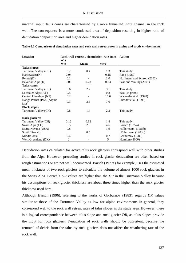
6. Discussion
137
material input, talus cones are characterised by a more funnelled input channel in the rock
wall. The consequence is a more condensed area of deposition resulting in higher ratio of
denudation / deposition area and higher denudation rates.
Table 6.2 Comparison of denudation rates and rock wall retreat rates in alpine and arctic environments.
Location Rock wall retreat / denudation rate (mm a-1)
Author
Min Mean Max Talus slopes: Turtmann Valley (CH) 0.2 0.7 1.3 This study Kärkevagge(N) 0.04 - 0.15 Rapp (1960) Reintal(D) 0.1 - 1.0 Hoffmann and Schrott (2002) Bavarian Alps (D) 0.06 0.28 0.73 Sass and Wollny (2001) Talus cones: Turtmann Valley (CH) 0.6 2.2 3.1 This study Lechtaler Alps (AT) 0.5 0.8 Sass (in press) Central Himalaya (NP) 3.2 - 15.6 Watanabe et al. (1998) Nanga Parbat (PK), (Alpine fans)
0.3 2.5 7.0 Shroder et al. (1999)
Block slopes: Turtmann Valley (CH) 0.8 1.4 2.3 This study Rock glaciers: Turtmann Valley(CH) 0.12 0.62 1.8 This study Swiss Alps (CH) 0.5 2.5 4.6 Barsch (1977a) Sierra Nevada (USA) 0.8 - 1,9 Höllermann (1983b) South Tirol (I) 0.5 Höllermann (1983b) Middle Asia 0.4 - 0.7 Gorburnov (1983) West Greenland (DK) 2 - 5 Humlum (2000)
Denudation rates calculated for active talus rock glaciers correspond well with other studies
from the Alps. However, preceding studies in rock glacier denudation are often based on
rough estimations or are not well documented. Barsch (1977a) for example, uses the estimated
mean thickness of two rock glaciers to calculate the volume of almost 1000 rock glaciers in
the Swiss Alps. Barsch’s DR values are higher than the DR in the Turtmann Valley because
his assumptions on rock glacier thickness are about three times higher than the rock glacier
thickness used here.
Although Barsch (1996), referring to the works of Gorburnov (1983), regards DR values
similar to those of the Turtmann Valley as low for alpine environments in general, they
correspond well to the rock wall retreat rates of talus slopes in the study area. However, there
is a logical correspondence between talus slope and rock glacier DR, as talus slopes provide
the input for rock glaciers. Denudation of rock walls should be consistent, because the
removal of debris from the talus by rock glaciers does not affect the weathering rate of the
rock wall.

7. Conclusion
138
7 Conclusion
The analysed and quantified storage landforms of the Turtmann Valley reveal a detailed
paraglacial evolution of this Alpine geosystem. The analysis of the spatial distribution of
storage landforms allows for a relative reconstruction of the Post Glacial land surface
evolution of the Turtmann Valley. Though partially based on assumptions, the applied
methods resulted in sediment volumes that allow calculating denudation rates in good
agreement to previous results for other Alpine environments. As previous sediment storage
analysis were performed whether in much smaller or much larger drainage basins, this study
bridges between these two extremes by analysing a meso scale catchment. Finally, the
importance of rock glaciers in the paraglacial evolution of the valley and the sediment storage
distribution stresses the role of periglacial processes in the sediment flux system of high
alpine environments. The main results of the study are as follows:
• The distribution of sediment storage landforms shows a distinct high Alpine pattern
and distribution structure.
• The relative and absolute positions of landforms within the sediment cascade together
with their spatial extent and volume hint on a sequence of landform development.
From this spatial pattern a relative model of paraglacial landform evolution can be
inferred.
• Slope sediment storage landforms cover more than 50% of the hanging valley surface,
followed by moraine deposits (38%) and rock glaciers (11%). Alluvial deposits and
large rock fall debris cover less than 2% of the land surface.
• Sediment volumes were modelled on two spatial scales: (1) in one hanging valley,
sediment volumes are based on extrapolation of sediment thickness information
derived by geophysical surveying. (2) For the entire Turtmann Valley, volumes are
calculated applying different approaches according to the four sediment flux
subsystems. Two scenarios of sediment volumes are proposed.
• Sediment storage is dominated by moraine deposits that include 77 or 60 % of the
volume according to scenario I and II, respectively. Between 18 (I) and 25% (II) of
debris is located on slopes, while 4 (I) or 15% (II) of sediment volume is stored in
rock glaciers.
• A total sediment volume of 1,030.7 ±515.3 x 10⁶ m3 (I) or 778.8 ±389.4 x 10⁶ m3 (I) is
stored in the Turtmann Valley. More than 70 % of the material is located in the

7. Conclusion
139
hanging valleys, 20% is found on the main valley lateral slopes, while the main trough
and the glacier forefield each contain 3% of the sediment volume.
• Relative sediment volumes per area in the hanging valleys exceed the volume per area
stored in the main valley trough.
• The hanging valleys subsystems are considered as closed with respect to the coarse
debris flux and consequently decoupled from the main valley system. Lateral valley
slopes and main valley floor are only coupled along avalanche corridors or creeks. The
glacier forefield was coupled with the main valley floor for most of the Holocene; the
closure of the forefield by the dam disconnected the sediment cascade of the glacial
sediment flux.
• A mean volume of 1997.6 ±998.8 and 1509.5 ±754.8 t km-2 a-1 was transported within
the Turtmann valley based on 10 ka of process activity for scenarios I and II,
respectively.
• The average denudation rate for the Turtmann Valley varies between 1.25 ±0.62 and
0.94 ±0.47 mm a-1 following scenarios I and II, respectively. The denudation rate for
the hanging valleys is slightly higher showing rates of 2.23 ±1.11 (I) and 1.45 ±0.71
(II) mm a-1. In contrast, volumes stored in the glacier forefield result in a mean
denudation rate of 0.13±0.07 mm a-1.
• Denudation rates for single processes range from 0.2–2.6 mm a-1 for talus deposits and
between 0.1 and 1.4 mm a-1 for active talus-derived rock glaciers.
• The paraglacial reworking of glacial deposits in the hanging valleys was accomplished
mainly by glacier-derived rock glaciers. Their distribution is used to generate a model
of relative paraglacial landform succession in the hanging valleys.
• The paraglacial period can be divided into three main phases: Today’s relict
glacier-derived rock glaciers and block slopes are the landforms that formed during
the earliest stage of the paraglacial period. Rock glaciers formed from deposits of a
first Late Glacial glacier maximum (probably from the Daun phase). Talus slopes and
inactive rock glaciers formed during a second stage, when deposits from a smaller
Late Glacial glacier advance were reworked (probably Egesen phase, Younger Dryas).
Active glacier-derived rock glaciers are the most recent last landforms that have
developed from glacial deposits in the hanging valleys of the Turtmann Valley during
the Holocene.
• Since most of the active rock glaciers are talus-derived, the reworking of paraglacial
deposits is most probably completed. Assumed that most of the current bedrock

7. Conclusion
140
weathering is not influenced any more by stress release following deglaciation, the
paraglacial period in the hanging valleys of the Turtmann Valley is considered to be
terminated.

8. Summary
141
8 Summary
Sediment flux plays a central role within the evolution of land surfaces and Earth’s
biogeochemical systems. Within sediment flux systems, the role of sediment storage is often
the least understood part. A quantification of storage volumes is often based on rough
assumptions. However, geophysical methods, high resolution digital terrain data and GIS
techniques open up new possibilities for the more accurate quantification of sediment storage
volumes.
This study analyses the spatial distribution of sediment storage landforms and quantifies
sediment volumes in the high alpine Turtmann Valley, Swiss Alps. A detailed
geomorphological mapping provided information on the spatial structure of storage
landforms. Geophysical methods were used to derive sediment thickness of storage landforms
in one hanging valley, known as the Hungerlitaelli. Sediment volumes of single landforms
were quantified in the Hungerlitaelli by extrapolating sediment thickness data into the entire
hanging valley. The sediment storage of the entire Turtmann Valley was assessed for the four
different sediment flux subsystems. Quantification of sediment stored in the hanging valleys
was performed by transferring the average sediment thickness of the different landforms
observed in the Hungerlitaelli hanging valley to landforms located in the other hanging
valleys. The valley floor volume was estimated using the SLBL method that excavates a
digital elevation model until an assumed glacial trough surface is formed. The sediment
storage volume of the glacier forefield was quantified by constructing an assumed bedrock
surface, while the storage volume on main valley slopes was estimated using an assumed
average sediment depth.
The distribution of sediment storage landforms reveals a typical high Alpine land surface
pattern. Slope sediment storage landforms cover more than 50% of the hanging valley surface,
followed by moraine deposits (38%) and rock glaciers (11%). Alluvial deposits and large rock
fall debris cover less than 2% of the land surface. Sediment volumes were quantified using
two scenarios. Scenario I considers the moraine debris layer buried underneath rock glaciers
and increases the amount of material stored in moraine deposits that is removed from the rock
glacier class. In scenario II the entire modelled volume of the rock glaciers is considered
causing less volume stored in moraine deposits and an increase in rock glacier storage.
Sediment storage is dominated by moraine deposits that include 77 or 60 % of the volume

8. Summary
142
according to scenario I and II, respectively. Between 18 (I) and 25% (II) of debris is located
on slopes, while 4 (I) or 15% (II) of sediment volume is stored in rock glaciers.
A total sediment volume of 1,030.7 ±515.3 x 10⁶ m3 (I) and 778.8 ±389.4 x 10⁶ m3 (II),
respectively is stored in the Turtmann Valley. More than 70 % of the material is located in the
hanging valleys, 20% is found on the main valley lateral slopes, while the main trough and the
glacier forefield each contains 3% of the sediment volume. The hanging valley subsystems
are considered as closed with respect to the coarse debris flux and consequently decoupled
from the main valley system. Lateral valley slopes and main valley floor are only coupled
along avalanche corridors or creeks. The glacier forefield was coupled with the main valley
floor for most of the Holocene; the closing of the forefield is caused by the dam disconnected
the sediment cascade of the glacial sediment flux.
The average denudation rate for the Turtmann Valley varies between 1.25 ±0.62 and 0.94
±0.47 mm a-1 following scenarios I and II, respectively. The denudation rate for the hanging
valleys is slightly higher showing rates of 2.23 ±1.11 (I) and 1.45 ±0.71 (II) mm a-1,
respectively. In contrast, volumes stored in the glacier forefield result in a mean denudation
rate of 0.13±0.07 mm a-1.
The relative and absolute positions of landforms within the sediment cascades together with
their spatial extent and volume hint on a sequence of landform development. From this spatial
pattern a relative model of paraglacial landform evolution can be inferred. A reworking of
glacial deposits in the hanging valleys was accomplished mainly by glacier-derived rock
glaciers. Their distribution is used to generate a model of relative paraglacial landform
succession in the hanging valleys. The paraglacial period can be divided into three main
phases: Today’s relict glacier-derived rock glaciers and block slopes are the landforms that
were build up during the earliest stage of the paraglacial period. Rock glaciers developed from
deposits of a first Late Glacial glacier maximum (probably Daun). Talus slopes and inactive
rock glaciers were created during a second stage, when deposits from a smaller Late Glacial
glacier advance were reworked (probably Egesen; Younger Dryas). Active glacier-derived
rock glaciers are the most recent landforms that have been developed from glacial deposits in
the hanging valleys of the Turtmann Valley during the entire Holocene.
Since most of the active rock glaciers are talus-derived, the reworking of paraglacial deposits
is probably completed. Assuming that most of the current bedrock weathering is not
influenced any more by stress release following deglaciation, the paraglacial period in the
hanging valleys of the Turtmann Valley is considered to be finished.
8. Summary
143
To conclude, the analysis of the spatial distribution of storage landforms allows for a relative
reconstruction of the Post Glacial land surface evolution of the Turtmann Valley. Though
partially based on assumptions the applied methods result in sediment volumes that allow
calculating denudation rates in good agreement to previous results for other Alpine
environments. As previous sediment storage analyses were performed, whether in much
smaller or much larger drainage areas, this study bridges between these two extreme by
analysing a meso scale catchment. Finally, the importance of rock glaciers in the paraglacial
evolution of the valley and the sediment storage distribution stresses the role of periglacial
processes in the sediment flux system of high alpine environments.

References
144
9 References
Arenson, L., Hoelzle, M. and Springman, S., 2002. Borehole deformation measurements and
internal structure of some rock glaciers in Switzerland. Permafrost and Periglacial
Processes, 13(2): 117-135.
Bakker, J.P. and LeHeux, W.N., 1952. A remarkable new geomorphological law. I. Physical
Geography, Series B, 55(4): 399-410.
Ballantyne, C.K., 2002a. A general model of paraglacial landscape response. Holocene, 12(3):
371-376.
Ballantyne, C.K., 2002b. Paraglacial Geomorphology. Quaternary Science Reviews, 21:
1935-2017.
Ballantyne, C.K., 2003. Paraglacial landform succession and sediment storage in deglaciated
mountain valleys: theory and applroaches to calibration. Zeitschrift für
Geomorphologie, Suppl.-Vol 132: 1-18.
Ballantyne, C.K. and Harris, C., 1994. The Periglaciation of Great Britain. Cambridge
University Press, Cambridge.323p
Ballantyne, C.K. and Benn, D.I., 1996. Paraglacial Slope Adjustment during recent
deglaciation and its implications for slope evolution in formerly glaciated
environments. In: M.G. Anderson and S.M. Brooks (Editors), Advances in hillslope
processes. Symposia Series. John Wiley & Sons, Chichester: 1173-1195.
Bansemer, K., 2004. Spätkänozoische Reliefentwicklung der Schweizer Alpen, University of
Bonn, Bonn, 135p.
Barsch, D., 1977a. Eine Abschätzung von Schuttproduktion und Schuttransport im Bereich
aktiver Blockgletscher der Schweizer Alpen. Zeitschrift für Geomorphologie N.F., 28:
148-160.
Barsch, D., 1977b. Nature and importance of mass-wasting by rock glaciers in alpine
permafrost environments. Earth Surface Processes, 2: 231-245.
Barsch, D., 1981. Ergebnisse der Heidelberg-Ellesmere Island-Expedition. Heidelberger
Geographische Arbeiten, 69. Geographisches Institut, Universität Heidelberg,
Heidelberg.
Barsch, D., 1996. Rockglaciers - Indicators for the present and former geoecology in high
mountain environments. Springer-Verlag, Heidelberg, 319p.

References
145
Barsch, D. and Caine, N.T., 1984. The nature of mountain geomorphology. Mountain
Research and Development, 4(4): 287-298.
Barsch, D. and Jakob, M., 1998. Mass transport by active rockglaciers in the Khumbu
Himalaya. Geomorphology, 26(1-3): 215-222.
Bearth, P., 1980. Geologischer Atlas der Schweiz. Blatt 1308 St. Niklaus, Erläuterungen,
Bern.50p.
Benn, D.I., Kirkbride, M.P., Owen, L.A. and Brazier, V., 2005. Glaciated valley landsystems.
In: D.A. Evans (Editor), Glacial Landsystems. Hodder Arnold, London,: 372-406.
Berthling, I., Elzelmuller, B., Isaksen, K. and Sollid, J.L., 2000. Rock glaciers on Prins Karls
Forland. II: GPR soundings and the development of internal structures. Permafrost and
Periglacial Processes, 11(4): 357-369.
Besson, O., Roullier, J.-D., Frei, W. and Masson, H., 1992. Campagne de sismique-réflexion
dans la Vallée du Rhône entre Sion et Martigny, Suisse. Bull. Murithienne, Sion, 18.
Beylich, A.A., Lindblad, K., Molau, U., Sandberg, O. and Wache, S., 2004. Intensity and
spatio-temporal variability of fluvial sediment transfers in arctic-oceanic Latnjavagge,
northernmost Swedish Lapland. Geophysical Research Abstracts, 6: 06807.
Bezinge, A., 1987. Glacal meltwater streams, hydrology and sediment transport: the case of
the Grande Dixence hydroelectric scheme. In: A.M. Gurnell and M.J. Clark (Editors),
1987. Wiley, Chichester: 473-498.
Bircher, W., 1983. Zur Gletscher- und Klimageschichte des Saastales. Glazialmorphologische
und dendroklimatologische Untersuchungen. Physische Geographie, 9.
Blaschke, T., 2000. Landscape metrics: Konzepte eines jungen Ansatzes der
Landschaftsökologie und Anwendungen in Naturschutz und Landschaftsforschung.
Arch. für Naturschutz und Landschaftsforschung, 39: 267-299.
Brunsden, D., 1996. Geomorphological events and landform change. Zeitschrift für
Geomorphologie N.F., 40(3): 273-288.
Brunsden, D. and Thornes, J.B., 1979. Landscape sensitivity and change. Transactions
Institute of British Geographers (New Series), 4(4): 463-484.
Büdel, J., 1977. Klima-Geomorphologie. Arbeiten aus der Kommission für Geomorphologie
der Bayerischen Akademie der Wissenschaften.
Burbank, D.W. and Anderson, R.S., 2005. Tectonic Geomorphology. Blackwell Science Ltd.,
Malden, Oxford, Carlton, 274 p.
Burger, K.C., Degenhardt, J.J. and Giardino, J.R., 1999. Engineering geomorphology of rock
glaciers. Geomorphology, 31(1-4): 93-132.
References
146
Caine, N., 1967. The texture of talus in Tasmania. Journal of Sedimentary Petrology, 37: 796-
803.
Caine, N.T., 1974. The geomorphic processes of the alpine environment. In: J.D. Ives and
R.G. Barry (Editors), Arctic and Alpine Environments. Methuen, London: 721-748.
Caine, N., 1986. Sediment movement and storage on alpine slopes in the Colorado Rocky
Mountains. In: A.D. Abrahams (Editor), Hillslope processes. Allen & Unwin, London:
115-137.
Caine, N., 2001. Geomorphic systems of Green Lakes Valley. In: W.D. Bowman and S. T.R.
(Editors), Structure and function of an alpine ecosystem. Oxford University Press,
Oxford: 45-74.
Caine, N., 2004. Mechanical and chemical denudation in mountain systems. In: L.A. Owen
and O. Slaymaker (Editors), Mountain Geomorphology. Arnold, London, pp. 132 -
152.
Caine, N. and Swanson, F.J., 1989. Geomorphic coupling of hillslope and channel systems in
two small mountain basins. Zeitschrift für Geomorphologie, 33(2): 189-203.
Campbell, D. and Church, M., 2003. Reconnaissance sediment budgets for the Lynn Valley,
British Columbia: Holocene and contemporary time scales. Canadian Journal of Earth
Science, 40: 701-713.
Chorley, R.J., 1962. Geomorphology and general systems theory. Geological Survey
Professional Paper, 500-B: 1-10.
Chorley, R.J. and Kennedy, B.A., 1971. Physical geography - A systems approach, London.
Church, M., 2002. Fluvial Sediment Transfer in Cold Regions. In: K. Hewitt, M.-L. Byrne,
M. English and G.J. Young (Editors), Landscapes of Transition. Kluwer, Dordrecht:
93-118
Church, M. and Ryder, J.M., 1972. Paraglacial sedimentation: a consideration of fluvial
processes conditioned by glaciation. Geol. Soc. Am. Bull., 83: 3059-3071.
Church, M. and Slaymaker, O., 1989. Disequilibrium of Holocene sediment yield in glaciated
British Columbia. Nature, 337(2): 452-454.
Chorley, R.J., Schumm, S.A. and Sudgen, D.E., 1984. Geomorphology, London, New
York.607p.
Cruden, D.M. and Hu, X.Q., 1993. Exhaustion and steady state models for predicting
landslide hazards in the Canadian Rocky Mountains. Geomorphology, 8: 279-285.
Cruden, D.M. and Hu, X.Q., 1996. The shape of some mountain peaks in the canadian
rockies. Earth Surface Processes, 24: 1229-1241.

References
147
Curry, A.M., 1999. Paraglacial modification of slope form. Earth Surface Processes and
Landforms, 24(13): 1213-1228.
Curry, A.M. and Morris, C.J., 2004. Lateglacial and Holocene talus slope development and
rockwall retreat on Mynydd Du, UK. Geomorphology, 58(1-4): 85-106.
Daniels, D.J., 1996. Surface-penetrating Radar, Radar, Sonar, Navigation and Avionics Series
6. Institute of Electrical Engineers, London, 300p.
De Boer, D.H., 2001. Self-organisation in fluvial landscapes: sediment dynamics as an
emergent property. Computers and Geosciences, 27: 995-1001.
deGroot-Hedlin, C. and Constable, S.C., 1990. Occams's inversion to generate smooth, two-
dimensional models from magnetotelluric data. Geophysics, 55: 1613-1624.
Dehn, M., Gärtner, H. & R. Dikau, 2001. Principles of semantic modeling of landform
structures. Computers and Geosciences, 27: 1005 - 1010.
Dietrich, W.E. and Dunne, T., 1978. Sediment budget for a small catchment in mountainous
terrain. Zeitschrift für Geomorphologie, Suppl. Bd. 29: 191-206.
Dietrich, W.E., Dunne, T., Humphrey, N.F. and L.M. Ried, 1982. Construction of sediment
budgets for drainage basins. In: F.J. Swanson, R.J. Janda, T. Dunne and D.N.
Swanston (Editors), Sediment Budgets and Routing in Forested Drainage Basins.
United States Department Agriculture Forest Service: 5-23.
Dikau, R., 1988. Entwurf einer geomorphographisch-analytischen Systematik von
Reliefeinheiten. Heidelberger Geographische Bausteine, 5.
Dikau, R., 1989. The application of a digital relief model to landform analysis in
geomorphology. In: J. Raper (Editor), Three dimensional applications in Geographical
Information Systems. Taylor & Francis, London: 51-77.
Dikau, R., 1998. The need for field evidence in modelling landform evolution. In: S.
Hergarten and H.J. Neugebauer (Editors), Process Modelling and Landform Evolution.
Lecture Notes in Earth Sciences. Springer-Verlag, Heidelberg: 3-12.
Dikau, R., Brunsden, D., Schrott, L. and Ibsen, M. (Editors), 1996. Landslide Recognition.
Identification, movement and causes. John Wiley & Sons Ltd, Chichester, 251 p.
Dymond, J.R., DeRose, R.C. and Harmsworth, G.R., 1995. Automated mapping of land
components from digital elevation data. Earth Surface Processes and Landforms, 20:
131-137.
Einsele, G., 2000. Sedimentary Basins: Evolution, Facies, and Sediment Budget. Springer,
Heidelberg.792p.

References
148
Einsele, G. and Hinderer, M., 1997. Terrestrial sediment yield and the lifetimes of reservoirs,
lakes, and larger basins. Geologische Rundschau, 86(2): 288-310.
Eisbacher, G.H. and Clague, J.J., 1984. Destructive Mass Movements in High Mountains:
Hazard and Management. 84-16, Geological Survey of Canada, 230p.
Escher, H., 1970. Bestimmung der klimatischen Schneegrenze in den Schweiz Alpen. .
Geographica Helvetica, 25: 35-43.
Etzelmüller, B., 2000. Quantification of thermo-erosion in pro-glacial areas - examples from
Svalbard. Zeitschrift für Geomorphologie N.F., 44(3): 343-361.
Evans, I.S., 1980. An integrated system of terrain analysis and slope mapping. Zeitschrift für
Geomorphologie, Supplement Band, 80: 274-295.
Eybergen, F.A., 1986. Glacier snout dynamics and contempory push moraine formation at the
Turtmannglacier, Switzerland, INQUA Symposium on Genesis & Lithology of Glacial
Deposits. Amsterdam: 217-231.
Favis-Mortlock, D.T., Boardman, J., Parsons, A.J. and Lascelles, B., 2000. Emergence and
erosion: A model for rill initiation and development. Hydrological Processes, 14(11-
12): 2173-2205.
Finckh, P. and Frei, W., 1991. Seismic reflection profiling in the Swiss Rhone valley. Part I:
seismic reflection field work, seismic processing and seismic results of the Roche-
Vouvry and Turtmann and Agarn lines. Eclogae Geologicae Helvetiae, 84(2): 345-
357.
Fookes, P.G., Sweeney, M., Manby, C.N.D. and Martin, R.P., 1985. Geological and
geotechnical engineering aspects of low-cost roads in mountainous terrain.
Engineering Geology, 21(1-2): 1-152.
Frauenfelder, R. and Kääb, A., 2000. Towards a palaeoclimatic model of rock-glacier
formation in the Swiss Alps. Annals of Glaciology, 31: 281-286.
French, H.M., 1996. The periglacial environment. Longmann, London, 341p.
Froese, D.G., Smith, D.G. and Clement, D.T., 2005. Characterizing large river history with
shallow geophysics: Middle Yukon River, Yukon Territory and Alaska.
Geomorphology, 67(3-4): 391-406.
Gamper, M. and Suter, J., 1982. Postglaziale Klimageschichte der Schweizer Alpen.
Geographica Helvetica, 2: 105-114.
Gorburnov, A.P., 1983. Rock glaciers of the mountains of middle Asia Proceedings of the 4th
International Conference on Permafrost. Fairbanks, Alaska. National Academic Press:
359-362.

References
149
Graf, W.L., 1970. The Geomorphology of the glacial valley cross section. Arctic and Alpine
Research, 2(4): 303-312.
Gude, M., Daut, G., Dietrich, S., Mäusbacher, R., Jonasson, C., Bartsch, A. and Scherer, D.,
2002. Towards an integration of process measurements, archive analysis and
modelling in geomorphology - the Kärkevagge experimental site, Abisko area,
Northern Sweden. Geografiska Annaler, 84 A(3-4): 205-212.
Gustavsson, M., Kolstrup, E. and Seijmonsbergen, A.C., 2006. A new symbol-and-GIS based
detailed geomorphological mapping system: Renewal of a scientific discipline for
understanding landscape development. Geomorphology, 77(1-2): 90-111.
Haas, P., 1978. Untersuchung zur Gletschergeschichte im Val d'Anniviers, University of
Zürich, 110p.
Haas, J.N., Richoz, I., Tinner, W. and Wick, L., 1998. Synchronous Holocene climatic
oscillations recorded on the Swiss Plateau and at timberline in the Alps. The
Holocene, 8(3): 301-309.
Haeberli, W. and Vonder Mühll, D., 1996. On the characteristic and possible origin of ice in
the rock glacier permafrost. Zeitschrift für Geomorphologie N.F., Suppl.-Bd. 104: 43-
57.
Haines-Young, R. and Chopping, M., 1996. Quantifying landscape structure: a review of
landscape indices and their application to forested landscapes. Progress in Physical
Geography, 20(4): 418-445.
Hallet, B., Hunter, L. and Bogen, J., 1996. Rates of erosion and sediment evacuation by
glaciers: A review of field data and their implications. Global and Planetary Change,
12: 213-235.
Harbor, J. and Warburton, J., 1993. Relative Rates of Glacial and Nonglacial Erosion in
Alpine Environments. Arctic and Alpine Research, 25(1): 1-7.
Hauck, C. and Vonder Mühll, D., 2003. Inversion and Interpretation of Two-Dimensional
Geoelectrical Measurements for Detecting Permafrost in Mountainous Regions.
Permafrost and Periglacial Processes, 14: 305-318.
Hauck, C., 2001. Geophysical methods for detecting permafrost in high mountains. VAW
Mitteilungen, 171. Versuchsantalt für Wasserbau Hydrologie und Glaziologie der
Eidgenössischen Technischen Hochschule,, Zürich, 204p.
Heim, A., 1932. Bergsturz und Menschenleben. Beiblatt zur Vierteljahrschrift, 20, Zürich,
218p.

References
150
Heiri, O., Lotter, A.F., Hausmann, S. and Kienast, F., 2003. A chironomid-based Holocene
summer air temperature reconstruction from the Swiss Alps. The Holocene, 13(4):
477-484.
Hewitt, K., 2002. Postglacial Landform and Sediment Associations in a Landslide-fragmented
River-system: The Transhimalayan Indus Streams, Central Asia. In: K. Hewitt, M.-L.
Byrne, M. English and G.J. Young (Editors), Landscapes of Transition. Kluwer,
Dordrecht: 63-91.
Hinderer, M., 2001. Late Quaternary denudation of the Alps, valley and lake fillings and
modern river loads. Geodinamica Acta, 14(4): 231-263.
Hoffmann, T. and Schrott, L., 2002. Modelling sediment thickness and rockwall retreat in an
Alpine valley using 2D-seismic refraction (Reintal, Bavarian Alps). Zeitschrift für
Geomorphologie, Supplement Band, 127: 153-173.
Hoffmann, T. and Schrott, L., 2003. Determining sediment thickness of talus slopes and
valley fill deposits using seismic refraction - a comparison of 2D interpretation tools.
Zeitschrift für Geomorphologie N.F., Suppl.-Bd. 132: 71-87.
Höllermann, P., 1983a. Verbreitung und Typisierung von Glatthängen, Mesoformen des
Reliefs im heitigen Periglazialraum: 241-260.
Höllermann, P., 1983b. Blockgletscher als Mesoformen der Periglazialstufe. Bonner
Geographische Abhandlungen, 67, Bonn, 73p.
Holzhauser, H. and Zumbühl, H.J., 1996. To the history of the Lower Grindelwald Glacier
during the last 2800 years - paleaosols, fossil wood and historical pictorial records -
new results. Zeitschrift für Geomorphologie, Suppl.-Bd 104: 95-127.
Holzhauser, H., Magny, M. and Zumbühl, H.J., 2005. Glacier and lake level variations in
west-central Europe over the last 3500 years. The Holocene, 15(6): 789-801.
Hormes, A., Muller, B.U. and Schluchter, C., 2001. The Alps with little ice: evidence for
eight Holocene phases of reduced glacier extent in the Central Swiss Alps. Holocene,
11(3): 255-265.
Hörsch, B., 2003. Zusammenhang zwischen Vegetation und Relief in alpinen
Einzugsgebieten des Wallis (Schweiz). Ein Multiskaliger GIS- und
Fernerkundungsansatz. Bonner Geographische Abhandlungen, 110. Asgard Verlag,
Sankt Augustin, 256p.
Hufschmidt, G., 2002. GIS-gestützte Modellierung von Sedimentspeichern als Komponenten
eines alpinen Geosystems (Reintal, Bayrische Alpen), University of Bonn, 106p.

References
151
Huggett, R.J. and Chessman, J., 2002. Topography and the Environment. Prentice Hall,
London. 274p.
Huggett, R.J., 2003. Fundamental of Geomorphology. Routledge, London, 386p.
Humlum, O., 2000. The geomorphic significance of rock glaciers: estimates of rock glacier
debris volumes and headwall recession rates in West Greenland. Geomorphology,
35(1-2): 41-67.
Hutchinson, M.F., 1989. A new procedure for gridding elevation and stream line data with
automatic removal of spurious pits. Journal of Hydrology, 106: 211-232.
Ikeda, A. and Matsuoka, N., 2006. Pebbly versus bouldery rock glaciers: Morphology,
structure and processes. Geomorphology, 73(3-4): 279-296.
Ivy-Ochs, S., Schlüchter, C., Kubik, P.W., Synal, H.A. and Kerschner, H., 1996. The
exposure age of an Egesen moraine at Julier Pass, Switzerland, measured with the
cosmogenic radionuclides Be-10, Al-26 and Cl-36. Eclogae Geologicae Helvetiae,
89(3): 1049-1063.
Jaboyedoff, M., Baillifard, F., Couture, R., Locat, J. and Locat, P., 2004. Towards preliminary
hazard assessment using DEM topographic analysis and simple mechanic modeling.
In: W.A. Lacerda, M. Erhlich, A.B. Fontoura and A. Sayo (Editors), Landslide
evaluation and stabilization. Balkema, Amsterdam: 191-197.
Jaboyedoff, M. and Derron, M.H., 2005. A new method to estimate the infilling of alluvial
sediment of glacial valleys using a sloping local base level. Geografia Fisica e
Dinamica Quaternaria, 28(1): 37-46.
Jäckli, H., 1957. Gegenwartsgeologie des bündnerischen Rheingebiets. Ein Beitrag zur
exogenen Dynamik alpiner Gebirgslandschaften. Geotechnische Serie, 36. Kümmerle
& Frey, Bern, 135p.
Johnson, R.M. and Warburton, J., 2002. Annual sediment budget of a UK mountain torrent.
Geografiska Annaler Series a-Physical Geography, 84A(2): 73-88.
Jomelli, V. and Francou, B., 2000. Comparing the characteristics of rockfall talus and snow
avalanche landforms in an Alpine environment using a new methodological approach:
Massif des Ecrins, French Alps. Geomorphology, 35(3-4): 181-192.
Jordan, P. and Slaymaker, O., 1991. Holocene sediment production in Lillooet river basin,
British Columbia: a sediment budget approach. Géographie Physique et Quaternaire,
45(1): 45-57.
Kearey, P., Brooks, M. and Hill, I., 2002. An Introduction to Geophysical Exploration.
Blackwell, London, 280p.

References
152
Kelly, M.A., Buoncristiani, J.F. and Schlüchter, C., 2004a. A reconstruction of the last glacial
maximum (LGM) ice-surface geometry in the western Swiss Alps and contiguous
Alpine regions in Italy and France. Eclogae Geologicae Helvetiae, 97(1): 57-75.
Kelly, M.A., Kubik, P.W., Von Blankenburg, F. and Schlüchter, C., 2004b. Surface exposure
dating of the Great Aletsch Glacier Egesen moraine system, western Swiss Alps, using
the cosmogenic nuclide 10 BE. Journal of Quaternary Science, 19(5): 431-441.
Kneisel, C., 2003. Permafrost in recently deglaciated glacier forefields measurements and
observations in the eastern Swiss Alps and northern Sweden. Zeitschrift Fur
Geomorphologie, 47(3): 289-305.
Kneisel, C., in press. Assessment of subsurface lithology in mountain environments using 2D
resistivity imaging. Geomorphology.
Kneisel, C., Lehmkuhl, F. and Winkler, S., 1998. Legende für geomorphologische
Kartierungen in Hochgebirgen (GMK Hochgebirge). Trierer Geographische Studien,
18.
Kneisel, C. and Hauck, C., 2003. Multi-method geophysical investigation of a sporadic
permafrost occurence. Zeitschrift für Geomorphologie, Suppl. -Vol. 132: 145-159.
Knödel, K., Krummel, H. and Lange, G., 1997. Geophysik. Handbuch zur Erkundung des
Untergrundes von Deponien und Altlasten. Springer-Verlag, Berlin, 1063p.
Knopp, F., 2001. Untersuchungen zum Sedimenthaushalt eines hochalpinen Hängetals im
Turtmanntal, Wallis, Schweiz, University of Bonn, 123p.
König, O., 2006. Korngrößenmuster auf Oberflächen alpiner Sedimentspeicher, University of
Bonn, Bonn, 130p.
Krautblatter, M. and Moser, M., 2005. The implications of a four-year quantitative rockfall
measurement for hazard assessment, risk mitigation and the design of protection
measures. Proceedings of the 15th Conference on Engineering Geology, Erlangen
April 6th to 9th: 67-72.
Krautblatter, M. and Hauck, C. (submitted): First DC-resistivity monitoring of permafrost in
solid rockwalls. Journal of Geophysical Research.
Krautblatter, M. Moser, M., Schrott, L. and Wolf, J. (submitted): A study on sediment yield
and geomorphic work comprising all rockfall magnitudes in an alpine catchment
(Reintal, German Alps). Geomorphology.
Kugler, H., 1964. Die geomorphologische Reliefanalyse als Grundlage großmaßstäbiger
geomorphologischer Kartierung. Wiss. Veröff. Dt. Inst. f. Landeskunde, 21/22: 541-
655.

References
153
Kugler, H., 1974. Das Georelief und seine kartographische Modellierung, Halle-Wittenberg,
514p.
Kuhlemann, J., Frisch, W., Szekely, B., Dunkl, I. and Kazmer, M., 2002. Post-collisional
sediment budget history of the Alps: tectonic versus climatic control. International
Journal of Earth Sciences, 91(5): 818-837.
Kühni, A. and Pfiffner, O.A., 2001. Drainage patterns and tectonic forcing: a model study for
the Swiss Alps. Basin Research, 13: 169-197.
Labhart, T.P., 2001. Geologie der Schweiz. Ott Verlag, Thun, 211p.
Leemann, A. and Niessen, F., 1994. Holocene glacial activity and climatic variations in the
Swiss Alps: reconstucting a continuous record from proglacial lake sediments. The
Holocene, 4(3): 259-268.
Lehmann, O., 1933. Morphologische Therorie der Verwitterung von Steinschlagwänden
Vierteljahresschrift Naturforsch. Ges. Zürich 78: 83-126.
Loke, M.H. and Barker, R.D., 1995. Least-squares deconvolution of apparent resistivity
pseudosections. Geophysics, 60(6): 1682-1690.
Löwner, M.O., 2005. Semantische Modellierung von geomorphologischen Objekten in einem
Geoinformationssystem (GIS) unter besonderer Berücksichtigung von Wänden und
steilen Hangbereichen, Unversity of Bonn, Bonn, 146p.
Luckman, B.H., 1976. Rockfalls and rockfall inventory data: Some observations from
Surprise Valley, Jasper National Park, Canada. Earth Surface Processes, 1: 287-298.
Maisch, M., 1982. Zur Gletscher- und Klimageschichte des alpinen Spätglazials. Geographica
Helvetica, 22: 93-104.
Maisch, M., Wipf, A., Denneler, B., Battaglia, J. and Benz, C., 1999. Die Gletscher der
Schweizer Alpen. Schlussbericht NFP 31. vdf, Zürich, 373p.
Martinerie, R., De Cesare, G., Jordan, F. and Boillat, J.-L., 2005. Gestion globale des
sédiments de la retenue de Tourtmagne. Génération et analyse de variantes. In: A.
Schleiss (Editor), INTERREG III B - Projet ALPRESERV, Gestion durable des
sédiments dans les réservoirs alpins. Sion, CH, 22. Laboratoire de Constructions
Hydraulique, Ecole Polytechnique Fédérale de Lausanne: 39-66.
Massey, D., 1999. Space-time, `science´, and relationship between physical geography and
human geograpy. Transactions of the Institute of British Geographers, 24: 261-276.
McGarigal, K., 2002. Lanscape pattern metrics. In: A.H. El-Shaarawi and W.W. Piegorsch
(Editors), Encyclopedia of Environmentrics. Wiley and Sons, Sussex: 1135-1142.

References
154
Milliman, J.D. and Meade, R.H., 1983. World-wide delivery of river sediment to the oceans.
Journal of Geology, 91(1): 1-21.
Milliman, J.D. and Syvistki, J.P., 1992. Geomorphic / tectonic control of sediment discharge
to the ocean: the importance of small mountainous rivers. The Journal of Geology,
100: 525-544.
Molnar, P. and England, P., 1990. Late Cenozoic uplift of mountain ranges and global climate
change: chicken or egg? Nature, 364: 29-34.
Molnar, P., 2003. Nature, nurture and landscape. Nature, 426: 612-614.
Molnar, P., 2004. Late cenozoic increase in accumulation rates of terrestrial sediment: How
might climate change have affected erosion rates? Annu. Rev. Earth Planet. Sci., 31:
67-89.
Moorman, B.J., Robinson, S.D. and Burgess, M.M., 2003. Imaging periglacial conditions
with ground-penetrating radar. Permafrost and Periglacial Processes, 14(4): 319-329.
Müller, H.-N., 1984. Spätglaziale Gletscherschwankungen in den westlichen Schweizer Alpen
(Simplon - Süd und Val de Nendaz, Wallis) und im Nordisländischen Tröllskagi,
University of Zürich, Zürich, 199p.
Musil, M., Maurer, H., Green, A.G., Horstmeyer, H., Nitsche, F.O., Vonder Mühll, D. and
Springman, S., 2002. Shallow seismic surveying of an Alpine rock glacier.
Geophysics, 67(6): 1701-1710.
National Snow and Ice Data Centre, 1999. World glacier inventory. World Glacier
Monitoring Service and National Snow and Ice Data Center/World Data Center for
Glaciology, Boulder, CO. Internet source.
Neukum, G., 2001. The airborne HRSC-AX cameras: evaluation of the technical concept and
presentation of application results after one year of operations. Photogrammetric
Week, 01: 117-131.
Nichols, K.K., Bierman, P.R., Caffee, M., Finkel, R. and Larsen, J., 2005. Cosmogenically
enabled sediment budgeting. Geology, 33(2): 133-136.
Nyenhuis, M., 2005. Permafrost und Sedimenthaushalt in einem alpinen Geosystem,
University of Bonn, 217p.
Otto, J.-C., 2001. Das geomorpholgische System des Turtmanntals (Wallis, Schweiz).
Formen, Substrate, Prozesse, University of Bonn, 133p.
Otto, J.-C. and Dikau, R., 2004. Geomorphic system analysis of a high mountain valley in the
Swiss Alps. Zeitschrift für Geomorphologie N.F., 48(3): 323-341.

References
155
Otto, J.-C. and Sass, O., 2006. Comparing geophysical methods for talus slope investigations
in the Turtmann valley (Swiss Alps). Geomorphology, 76(3-4): 257-272.
Owens, P.N. and Slaymaker, O., 1992. Late Holocene sediment yield in small alpine and
subalpine drainage basins, British Columbia, Erosion, Debris Flows and Environments
in Mountain Regions (Proceedings of the Chengdu Symposium, July 1992). IAHS
publ.: 147-154.
Owen, L.A. and England, J., 1998. Observations on rock glaciers in the Himalayas and
Karakoram Mountains of northern Pakistan and India. Geomorphology, 26(1-3): 199-
213.
Owens, P.N. and Slaymaker, O. (Editors), 2004. Mountain Geomorphology. Edward Arnold
Publishers Limited, London, 313p.
Peizhen, Z., Molnar, P. and Downs, W.R., 2001. Increased sedimentation rates and grain sizes
2 - 4 Myr ago due to the influence of climate change on erosion rates. Nature, 410:
891-897.
Penck, A. and Brückner, E., 1909. Die Alpen im Eiszeitalter. Tauschnitz, Leipzig, 393p.
Penck, A., 1894. Morphologie der Erdoberfläche. Engelhorn, Stuttgart, 471p.
Perez, F.L., 1993. Talus movement in the high equatorial Andes: A synthesis of ten years of
data. Permafrost and Periglacial Processes, 4: 199-215.
Pfeffer, G., 2000. Untersuchungen zur Permafrostverbreitung mit geophysicalischen
Methoden im Turtmanntal/Wallis, University of Bonn, 118p.
Pfiffner, O.A., Lehner, P., Heitzmann, P., Mueller, S. and Steck, A., 1997a. Deep structure of
the Swiss Alps. Birkhäuser, 460p.
Pfiffner, O.A., Heitzmann, P., Lehner, P., Frei, W., Pugin, P. and Felber, M., 1997b. Incision
and backfilling of the Alpine valleys: Pliocene and Holocene processes. In: O.A.
Pfiffner, P. Lehner, P. Heitzmann, S. Mueller and A. Steck (Editors), Deep structure of
the Swiss Alps. Results of NRP 20. Birkhäuser, Basel: 265-288.
Phillips, J.D., 1986. Sediment storage, Sediment yield, and time scales in landscape
denudation studies. Geographical Analysis, 18(2): 161-167.
Phillips, J.D., 2003. Sources of nonlinearity and complexity in geomorphic systems. Progress
in Physical Geography, 27(1): 1-23.
Pinter, N. and Brandon, M.T., 1997. How erosion builds mountains. Scientific american, 4:
74-79.
Rahn, M., 1991. Eclogites from the Minugrat, Siviez-Mischabel nappe (Valais, Switzerland).
Schweiz. Mineral. Petrogr. Mitt., 71: 415-426.

References
156
Rapp, A., 1960. Recent Development of mountain slopes in Kaerkevagge and surroundings,
Northern Scandinavia. Geografiska Annaler, A 42(2-3): 1-200.
Rasemann, S., 2004. Geomorphometrische Struktur eines mesoskaligen alpinen Geosystems.
Bonner Geographische Abhandlungen, Bd. 111. Asgard-Verlag, Sankt Augustin.
Reid, L.M. and Dunne, T. (Editors), 1996. Rapid evaluation of sediment budgets. GeoEcology
paperback. Catena Verlag, (GeoScience Publisher), Reiskirchen, 164p.
Reynolds, J.M., 1997. An introduction to applied and environmental geophysics. John Wiley
& Sons, Chichester, 792p.
Richter, E., 1901. Geomorphologische Untersuchungen in den Hochalpen. Petermanns
Geographische Mitteilungen, 24: 1-103.
Roer, I., 2005. Rockglacier kinematics in a high mountain geosystem, University of Bonn,
217p.
Rosselli, A. and Olivier, R., 2003. Modélisation gravimétrique 2.5D et cartes des isohypses au
1:100,000 du substratum de la vallée du Rhone entre Villeneuve et Brig (Suisse).
Eclogae Geologicae Helvetiae, 96: 399-423.
Rothenbühler, C., 2003. Erfassung und Darstellung der Geomorphologie im Gebiet Bernina
(GR) mit Hilfe von GIS. In: M. Maisch, Vonder Mühll, D. & Monbaron, M. (Editor),
Entwicklungstendenzen und Zukunftsperspektiven in der Geomorphologie.
Publikation zur Jahrestagung der Schweizerischen Geomorphologischen Gesellschaft
(SGmG) anlässlich des 180. Jahreskongresses der Schweizerischen Akademie der
Naturwissenschaften (SANW) in Winterthur. Physische Geographie. Geographisches
Institut Zürich, Zürich: 117-126.
Röthlisberger, F., 1976. Gletscher- und Klimageschichte im Raum Zermatt, Ferpècle und
Arolla. . In: W. Scheebeli and F. Röthlisberger (Editors), 8000 Jahre Walliser
Gletschergeschichte. Schweizer Alpen Club, Bern: 59-150.
Sandmeier, K.J., 2005. REFLEXW Manual, Karlsruhe, 194p.
Sass, O., in Press. Determination of the internal structure of alpine talus deposits using
different geophysical methods (Lechtaler Alps, Austria). Geomorphology, Corrected
Proof.
Sass, O. and Wollny, K., 2001. Investigations regarding alpine talus slopes using ground-
penetration radar (GPR) in the Bavarian Alps, Germany. Earth Surface Processes and
Landforms, 26: 1071-1086.
Sass, O. and Krautblatter, M. (accepted). Debris-flow-dominated scree slopes: genetic models
derived from GPR measurements. Geomorphology.

References
157
Sass, O., Bell, R. and Glade, T., in press. Comparison of Georadar, 2D-resistivity and
traditional techniques for the subsurface exploration of landslides. Geomorphology.
Sass, O., Krautblatter, M. and Viles, H. (submitted). Short and long term measurements of
rockwall retreat over the Holocene in Nant Ffrancon, Snowdonia, Wales. Earth
Surface Process and Landform.
Schaller, M., von Blankenburg, F., Hovius, N. and Kubik, P.W., 2001. Large-scale erosion
rates from in situ-produced cosmogenic nuclides in European river sediments. Earth
and Planetary Science Letters, 188: 441-458.
Schiefer, E., Slaymaker, O. and Klinkenberg, B., 2001. Physiographically controlled
allometry of specific sediment yield in the Canadian Cordillera: A lake sediment-
based approach. Geografiska Annaler Series a-Physical Geography, 83A(1-2): 55-65.
Schindler, C., Cuenod, Y., Eisenlohr, T. and Joris, C.L., 1993. The Events of Randa, April
18th and May 9th, 1991 - an Uncommon Type of Rockfall. Eclogae Geologicae
Helvetiae, 86(3): 643-665.
Schlüchter, C. and Jörin, U., 2004. Alpen ohne Gletscher? Holz- und Torffunde als
Klimaindikatoren. Die Alpen, 6: 34-47.
Schlunegger, F., 1999. Controls of surface erosion on the evolution of the Alps: Constraints
from the stratigraphies of the adjacent foreland basins. International Journal of Earth
Sciences, 88(2): 285-304.
Schlunegger, F. and Hinderer, M., 2001. Crustal uplift in the Alps: Why the drainage pattern
matters. Terra Nova, 13(6): 425-432.
Schlyter, P., 1993. Geomorphic process studies related to climate change in Karkevagge,
northern Sweden - status of current research. Geografiska Annaler, Series A, 75
A(1-2): 55-60.
Schmidt, J. and Hewitt, A., 2004. Fuzzy land element classification from DTMs based on
geometry and terrain position. Geoderma, 121(3-4): 243-256.
Schmidt, J., Evans, I.S. and Brinkmann, J., 2003. Comparison of polynomial models for land
surface curvature calculation. International Journal of Geographical Information
Science, 17(8): 797-814.
Schneevoigt, N.J. and Schrott, L., 2006. Fernerkundungsbasierte Reliefformenerkennung im
Hochgebirge (Reintal, Bayerische Alpen) Geographica Helvetica, 3.
Schneider, M. and Otto, J.C., in press. A new semi-automatic tool for three dimensional
landform mapping, High Mountain Remote Sensing Cartography (HMRSC-IX). Graz.

References
158
Schrott, L. and Adams, T., 2002. Quantifying sediment storage and Holocene denudation in
an Alpine basin, Dolomites, Italy. Zeitschrift für Geomorphologie N.F. Suppl.-Bd.,
128: 129-145.
Schrott, L., Niederheide, A., Hankammer, M., Hufschmidt, G. and Dikau, R., 2002. Sediment
storage in a mountain catchment: geomorphic coupling and temporal variability
(Reintal, Bavarian Alps, Germany). Zeitschrift für Geomorphologie, 127: 175-196.
Schrott, L., Hufschmidt, G., Hankammer, M., Hoffmann, T. and Dikau, R., 2003. Spatial
distribution of sediment storage types and quantification of valley fill deposits in an
alpine basin, Reintal, Bavarian Alps, Germany. Geomorphology, 55: 45 - 63.
Schumm, S.A., 1979. Geomorphic thresholds: the concept and ist application. Transactions
Institute of British Geographers (New Series), 4(4): 485-515.
Schumm, S.A. and Lichty, R.W., 1965. Time, space, and casuality in geomorphology.
American Journal of Science, 263(February): 110-119.
Schweizerische Gesellschaft für Ur- und Frühgeschichte, 1993. Die Schweiz vom
Paläolithikum bis zum frühen Mittelalter - Paläolithikum und Mesolithikum, 1. Verlag
Schweizerische Gesellschaft für Ur- und Frühgeschichte, Basel, 302p.
Seijmonsbergen, A.C. and de Graaff, L.W.S., 2006. Geomorphological mapping and
geophysical profiling for the evaluation of natural hazards in an alpine catchment.
Natural Hazards and Earth System Science, 6(2): 185-193.
Shary, P.A., Sharaya, L.S. and Mitusov, A.V., 2002. Fundamental quantitative methods of
land surface analysis. Geoderma, 107(1-2): 1-32.
Shroder, J.F., Scheppy, R.A. and Bishop, M.P., 1999. Denudation of small alpine basins,
Nanga Parbat Himalaya, Pakistan. Arctic Antarctic and Alpine Research, 31(2): 121-
127.
Shroder, J.F. and Bishop, M.P., 2004. Mountain geomorphic systems. In: M.P. Bishop and
J.F. Shroder (Editors), Geographic Information Science and Mountain
Geomorphology. Springer, Berlin, pp. 33-74.
Slaymaker, O., 1991. Mountain geomorphology: a theoretical framework for measurement
programms. Catena, 18: 427-437.
Slaymaker, O., 2004. Mountain Geomorphology. In: A.S. Goudie (Editor), Encyclopedia of
Geomorphology. Routledge, London: 701-703.
Slaymaker, O. and Spencer, T., 1998. Physical Geography and Global Environmental Change.
Understanding Global Environmental Change. Addison Wesley Longman Limited,
Essex, 292p.

References
159
Slaymaker, O., Souch, C., Menounos, B. and Filippelli, G., 2003. Advances in Holocene
mountain geomorphology inspired by sediment budget methodology. Geomorphology,
55(1-4): 305-316.
Small, R.J., 1987. Moraine sediment budgets. In: A.M. Gurnell and M.J. Clark (Editors),
Glacio-fluvial sediment transfer - An alpine perspective. John Wiley & Sons Ltd.,
Chichester, New York, pp. 165-198.
Spedding, N., 1997. On growth and form in geomorphology. Earth Surface Processes and
Landforms, 22: 261-265.
Speight, J.G., 1974. A parametric approach to landform regions. Instit.Brit.Geography Special
Publication, 7: 213-230.
Speight, J.G., 1990. Landform. In: R.C. McDonald, R.F. Isbell, J.G. Speight, J. Walker and
M.S. Hopkins (Editors), Australian soil and land survey field handbook, pp. 8-42.
Stäblein, G., 1980. Die Konzeption der Geomorphologischen Karten GMK 25 und GMK 100
im DFG-Schwerpunktprogramm. Berliner Geographische Abhandlung, 31: 13-30.
Stäblein, G., 1984. Geomorphic altitudinal zonation in the arctic-alpine mountains of
Greenland. Mountain Research and Development, 4: 319-331.
Summerfield, M.A., 1996. Understanding landscape development: the evolving interface
between geomorpholgy and other earth sciences. Area, 28(2): 211-220.
Summerfield, M.A. and Kirkbride, M.P., 1992. Climate and landscape response. Nature, 355:
306.
Troll, C., 1966. Über das Wesen der Hochgebirgsnatur. In: C. Troll (Editor), Ökologische
Landschaftsforschung und vergleichende Hochgebirgsforschung. Erdkundliches
Wissen. Franz Steiner Verlag, Stuttgart: 127-151.
Tucker, G.E. and Slingerland, R., 1996. Predicting sediment flux from fold and thrust belts.
Basin Research, 8: 329-349.
van Asselen, S. and Seijmonsbergen, A.C., Expert-driven semi-automated geomorphological
mapping for a mountainous area using a laser DTM. Geomorphology, In Press.
van der Meer, J.J.M. and van Tatenhove, G.M., 1992. Drumlins in a full alpine setting: some
examples from Switzerland. Geomorphology, 5(6): 59-67.
van Steijn, H., 2002. Long-term landform evolution: Evidence from talus studies. Earth
Surface Processes and Landforms, 27(11): 1189-1199.
van Tatenhove, F. and Dikau, R., 1990. Past and present permafrost distribution in the
Turtmanntal, Wallis, Swiss Alps. Arctic and Alpine Research, 22(3): 302-316.

References
160
Vezzoli, G., 2004. Erosion in the Western Alps (Dora Baltea Basin): 2. Quantifying sediment
yield. Sedimentary Geology, 171: 247-259.
von Elverfeld, K., 2001. Analyse der Blockgletscher-Kinematik im Turtmanntal (Wallis,
Schweiz) mittels digitaler Photogrammetrie, University of Bonn.114p.
Wasson, R.J., 1996. What approach to the modelling of catchment scale erosion and sediment
transport shuld be adopted? In: W. Summer and D.E. Walling (Editors), Modelling
erosion, sediment transport and yield. . UNESCO Technical Documents in Hydrology
60. UNESCO: 1-11.
Watanabe, T., Dali, L. and Shiraiwa, T., 1998. Slope denudation and the supply of debris to
cones in Langtang Himal, Central Nepal Himalaya. Geomorphology, 26(1-3): 185-
197.
Whalley, W.B., 1974. The mechanics of high mountain - low frequency rock failure and its
importance in mountainous areas. Geographical Papers, 27: 48.
Wheeler, D.A., 1984. Using parabolas to describe the cross-sections of glaciated valleys.
Earth Surface Processes, 9: 391-394.
Wolff, I., 2006. Spätglacial und holozäne Gletscherstände im Turtmanntal, Wallis, Schweiz,
University of Bonn, Department of Geography, 130p.

Appendix
A
10 Appendix
A. Seismic refraction modelling results
SR04_1
SR04_2

Appendix
B
SR04_3

Appendix
C
SR04_4

Appendix
D
SR04_5l
SR04_5r

Appendix
E
Sr04_6o
SR04_6u

Appendix
F
SR04_7
SR04_7q

Appendix
G
SR04_9
SR05_1

Appendix
H
SR05_2
SR05_3

Appendix
I
SR05_4
SR05_5

Appendix
J
SR05_6

Appendix
K
SR05_7
SR05_8
SR05_9

Appendix
L
SR05_10
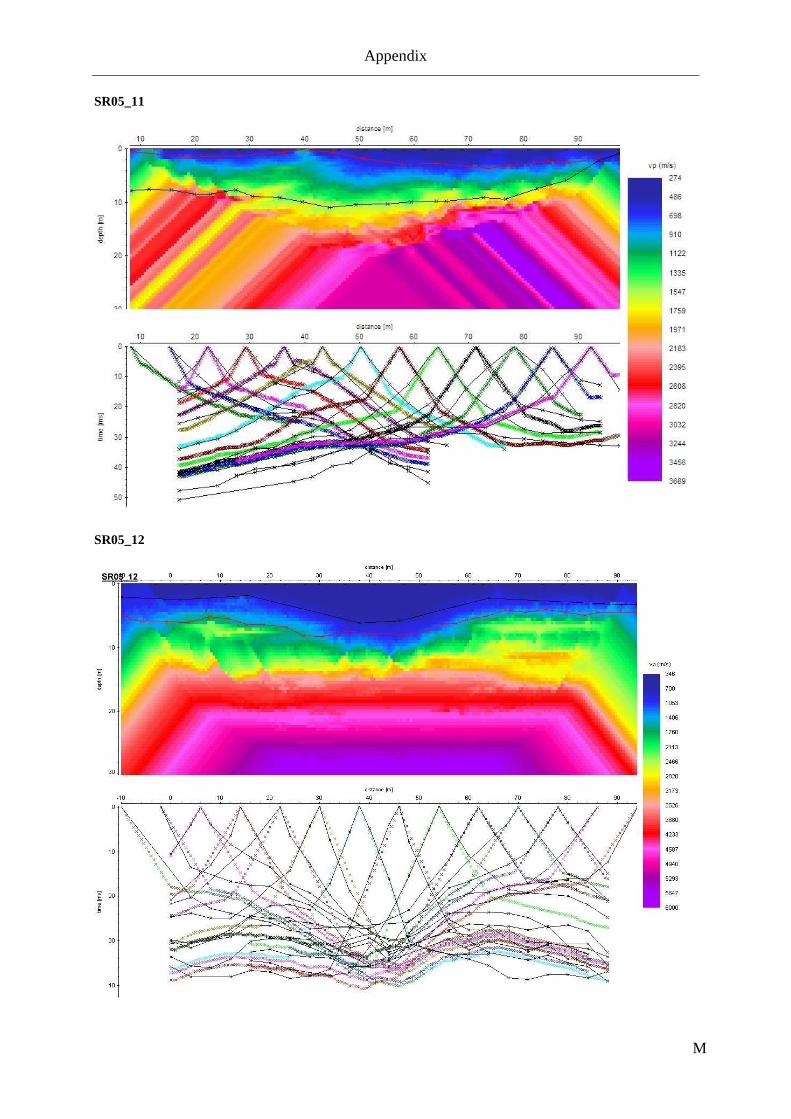
Appendix
M
SR05_11
SR05_12

Appendix
N
SR05_13
SR05_14
SR05_15
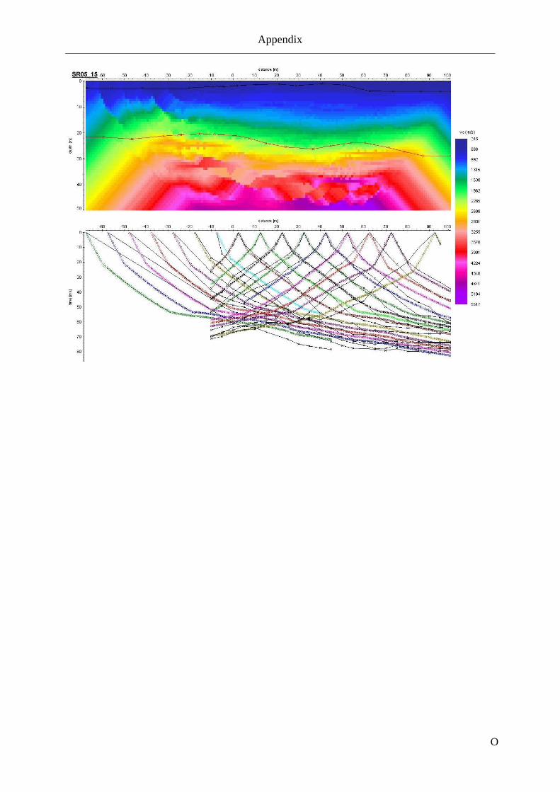
Appendix
O

Appendix
P
B. 2D-resistivity inversion results
10 20 30 40 50 60 70 80 90 100 110 120
2540
2550
2560
2570
2580
2590
2600
2610
2620
2630
0
2,000
3,000
4,000
5,000
7,500
10,000
12,500
15,000
20,000
25,000
30,000
50,000
75,000
100,000
ER04_1 Iteration 16 - RMS Error: 7.9 % Unit Spacing: 3 m
Resistivity in Ohm m
20 40 60 80 100 120
2580
2600
2620
2640
2660
0
2,000
3,000
4,000
5,000
7,500
10,000
12,500
15,000
20,000
25,000
30,000
50,000
75,000
100,000
ER04_2 Iteration 12 - RMS Error: 4.8 % Unit Spacing: 4 m Resistivity in Ohm m
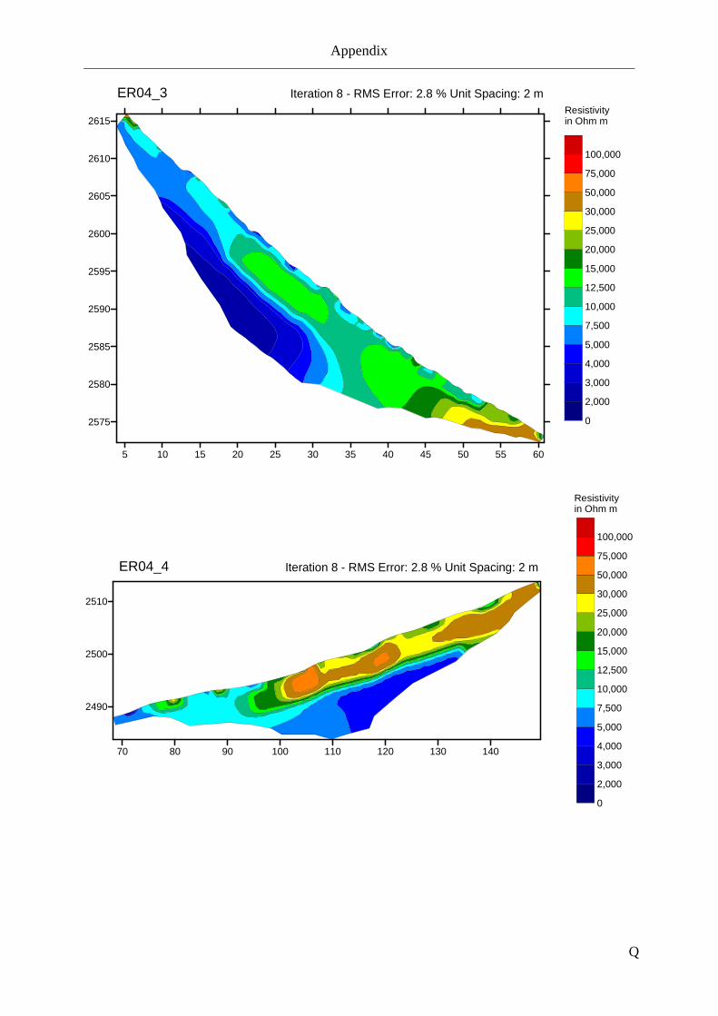
Appendix
Q
5 10 15 20 25 30 35 40 45 50 55 60
2575
2580
2585
2590
2595
2600
2605
2610
2615
0
2,000
3,000
4,000
5,000
7,500
10,000
12,500
15,000
20,000
25,000
30,000
50,000
75,000
100,000
ER04_3 Iteration 8 - RMS Error: 2.8 % Unit Spacing: 2 mResistivity in Ohm m
70 80 90 100 110 120 130 140
2490
2500
2510
0
2,000
3,000
4,000
5,000
7,500
10,000
12,500
15,000
20,000
25,000
30,000
50,000
75,000
100,000
ER04_4 Iteration 8 - RMS Error: 2.8 % Unit Spacing: 2 m
Resistivity in Ohm m

Appendix
R
-80 -60 -40 -20 0 20 40 60
2500
2520
2540
2560
2580
0
2,000
3,000
4,000
5,000
7,500
10,000
12,500
15,000
20,000
25,000
30,000
50,000
75,000
100,000
ER04_5 Iteration 13 - RMS Error: 11.8 % Unit Spacing: 5 mResistivity in Ohm m
20 40 60 80 100 120 140 160
2550
2560
2570
0
2,000
3,000
4,000
5,000
7,500
10,000
12,500
15,000
20,000
25,000
30,000
50,000
75,000
100,000
ER04_5q / 5q2 combined Iteration 7 - RMS Error: 8.8 % Unit Spacing: 3 m
Resistivity in Ohm m
Overlap

Appendix
S
10 20 30 40 50 60 70 80 90 100
2420
2430
2440
0
2,000
3,000
4,000
5,000
7,500
10,000
12,500
15,000
20,000
25,000
30,000
50,000
75,000
100,000
ER04_6 Iteration 6 - RMS Error 16.0% Unit spacing 3m
Resistivityin Ohm m
Resistivitiesin Ohm m
Iteration 5 - RMS Error = 8.4 % Unit Spacing 3m
10 20 30 40 50 60 70
2830
2840
2850
2860
2870
2880
0
2,000
3,000
4,000
5,000
7,500
10,000
12,500
15,000
20,000
25,000
30,000
50,000
75,000
100,000
ER05_1

Appendix
T
ER05_2 Resistivitiesin Ohm m
Iteration 5 - RMS Error = 5.4 % Unit Spacing 3m
10 20 30 40 50 60 70 80 90 100 110
2810
2820
2830
2840
2850
2860
2870
2880
2890
0
2,000
3,000
4,000
5,000
7,500
10,000
12,500
15,000
20,000
25,000
30,000
50,000
75,000
100,000
20 40 60 80 100 120 140 160
2720
2740
2760
0
2,000
3,000
4,000
5,000
7,500
10,000
12,500
15,000
20,000
25,000
30,000
50,000
75,000
100,000
ER05_4
Resistivitiesin Ohm m
Iteration 4 -RMS Error = 4.4 % Unit Spacing 4 m

Appendix
U
20 40 60 80 100 120
2680
2700
2720
0
2,000
3,000
4,000
5,000
7,500
10,000
12,500
15,000
20,000
25,000
30,000
50,000
75,000
100,000ER05_4
Resistivitiesin Ohm m
Iteration 3 - RMS Error = 27.4 % Unit Spacing 4m
20 40 60 80 100 120
2780
2800
0
2,000
3,000
4,000
5,000
7,500
10,000
12,500
15,000
20,000
25,000
30,000
50,000
75,000
100,000
ER05_5
Resistivitiesin Ohm m
Iteration 5 RMS Error = 11.4 % Unit Spacing 4m

Appendix
V
20 40 60 80 100 120 140 160 180
2580
2600
0
2,000
3,000
4,000
5,000
7,500
10,000
12,500
15,000
20,000
25,000
30,000
50,000
75,000
100,000ER05_6
Resistivitiesin Ohm m
Iteration 8 RMS Error = 11.4 % Unit Spacing 5 m
C. Ground penetrating radar images
GPR04_2
GPR04_3

Appendix
W
GPR04_5

Appendix
X
GPR05_6

Appendix
Y
2D-resitivity inversion parameters
Inversion settings
Initial damping factor 0.3
Minimum damping factor 0.1
Line search option 2
Convergence limit 5
Minimum change in RMS error 0.4
Number of iterations 5
Vertical to horizontal flatness filter ratio 0.5
Model for increase in thickness of layers 2
Number of nodes between adjacent electrodes 2
Flatness filter type, Include smoothing of model resistivity 1
Reduce number of topographical datum points? 0
Carry out topography modeling? 1
Type of topography trend removal 1
Type of Jacobian matrix calculation 1
Increase of damping factor with depth 1.2
Type of topographical modeling 4
Robust data constrain? 1
Cutoff factor for data constrain 0.05
Robust model constrain? 1
Cutoff factor for model constrain 0.005
Allow number of model parameters to exceed datum points? 1
Use extended model? 0
Reduce effect of side blocks? 2
Type of mesh 2
Optimise damping factor? 1
Time-lapse inversion constrain 0
Type of time-lapse inversion method 0
Thickness of first layer 0.5
Factor to increase thickness layer with depth 1.1
USE FINITE ELEMENT METHOD (YES=1,NO=0) 1
WIDTH OF BLOCKS 1
MAKE SURE BLOCKS HAVE THE SAME WIDTH 1
RMS CONVERGENCE LIMIT (IN PERCENT) 1
USE LOGARITHM OF APPARENT RESISTIVITY 0
LIMIT RESISTIVITY VALUES(0=No,1=Yes) 1
Upper limit factor (10-50) 20
Lower limit factor (0.02 to 0.1) 0.05
Type of reference resistivity (0=average,1=first iteration) 0
Model refinement (1.0=Normal,0.5=Half-width cells) 0.5
Combined Combined Marquardt and Occam inversion 0
Type of optimisation method 0
Convergence limit for Incomplete Gauss-Newton method 0.005
Use data compression with Incomplete Gauss-Newton 0

Appendix
Z
Use reference model in inversion (0=No,1=Yes) 0
Damping factor for reference model 0.005
Use fast method to calculate Jacobian matrix. 1
Use higher damping for first layer? (0=No,1=Yes) 0
Extra damping factor for first layer 1.5
Type of finite-element method 0