1

Paradoxical Euler: Integrating by Differentiating

Andrew Fabian Hieu D. Nguyen

Department of Mathematics

Rowan University, Glassboro, NJ 08028 February 12, 2012

I. Introduction

Every student of calculus learns that one typically solves a differential equation by integrating it. However, as Euler showed in his 1758 paper (E236), Exposition de quelques paradoxes dans le calcul intégral (Explanation of certain paradoxes in integral calculus) [2], there are differential equations that can be solved by actually differentiating them again. This initially seems paradoxical or as Euler describes it in the introduction of his paper:

Here I intend to explain a paradox in integral calculus that will seem rather strange: this is that we sometimes encounter differential equations in which it would seem very difficult to find the integrals by the rules of integral calculus yet are still easily found, not by the method of integration, but rather in differentiating the proposed equation again; so in these cases, a repeated differentiation leads us to the sought integral. This is undoubtedly a very surprising accident, that differentiation can lead us to the same goal, to which we are accustomed to find by integration, which is an entirely opposite operation.

A discussion of Euler’s paradoxical method and the geometrical problems that are solved

in his paper appears in our synopsis [3] (available on the Euler Archive) and also in Edward Sandifer’s column, How Euler Did it, Oct 2008 [5]. In this paper, we revisit Euler’s paradoxical method, discuss one of his geometrical problems (Problem I), and reformulate it using vectors in order to demonstrate that his method is a standard technique used by modern differential geometers today. Moreover, we investigate an interesting generalization of Problem I involving pedal curves to pedal surfaces and more generally to pedal manifolds. This leads to the notion of tangentially equidistant surfaces, which contains an interesting family of developable ruled surfaces. II. Integrating by Differentiating

In his E236 paper [2], Euler presents four geometrical problems (I-IV) to demonstrate his paradoxical method of differentiation. We shall discuss only the first problem:

PROBLEM I Given point A, find the curve EM such that the perpendicular AV, derived from point A onto some tangent of the curve MV, is the same size everywhere (Figure 1).

2

Figure 1

In modern terms, Problem I asks for a curve EM where every one of its tangent lines has fixed distance from point A (origin).

To solve this problem, Euler begins by introducing notation. In Figure 1, let α denote the curve EM and set x AP= , y PM= , dx Pp Mm= = , dy mπ= , and 2 2ds Mm dx dy= = + . It follows from the similarity of the three triangles APRV , PMSV , and MmπV that

,PS M PR mPM Mm AP Mm

π π= = ,

which implies

,PM M ydx AP m xdyPS PRMm ds Mm ds

π π⋅ ⋅= = = = .

Thus,

ydx xdya AV PS PRds−= = − = ,

or in differential form, 2 2ydx xdy a dx dy− = + . (1.1)

To solve (1.1), Euler applies the “ordinary” method of integrating a differential equation. Towards this end, he squares (1.1) to obtain 2 2 2 2 2 2 2 22y dx xydxdy x dy a dx a dy− + = + and then solves for dy by extracting square roots:

2 2 2

2 2

xydx adx x y ady

a x− + + −

=−

.

This is equivalent to 2 2 2 2 2a dy x dy xydx adx x y a− + = + − . (1.2)

Next, Euler applies the substitution 2 2y u a x= − to (1.2), and by assuming 2 2x a≠ (otherwise 0)y = , he obtains

2 2 2( ) 1a x du adx u− = − . (1.3)

3

Now, it is straightforward to check that 2 1u = is a solution to (1.3) since 0du = . Therefore, 2 2y a x= ± − , or upon squaring both sides, yields the circle of radius a centered at the origin as the solution (see Figure 2): 2 2 2x y a+ = . (1.4)

Figure 2

On the other hand, if 2 1u ≠ , then (1.3) can be separated as

2 22 1du adx

a xu=

−−,

and upon integration Euler reveals a family of lines as the other solution to Problem I:

2 2( 1) ( 1)2 2n ny x an n− += + . (1.5)

Here, n is a constant of integration. Observe that the lines described by (1.5) are all tangent to the circle in (1.4) (see Figure 3) and reveals the circle as their envelope (see Figure 4).

Figure 3 Figure 4

4

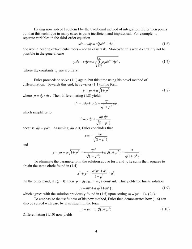
Having now solved Problem I by the traditional method of integration, Euler then points

out that this technique in many cases is quite inefficient and impractical. For example, to separate variables in the third-order equation 3 33ydx xdy a dx dy− = + , (1.6) one would need to extract cube roots – not an easy task. Moreover, this would certainly not be possible in the general case

0

nn k kn k

ky dx xdy a c dx dy−

=

− = ∑ , (1.7)

where the constants kc are arbitrary.

Euler proceeds to solve (1.1) again, but this time using his novel method of differentiation. Towards this end, he rewrites (1.1) in the form 21y px a p= + + (1.8) where /p dy dx= . Then differentiating (1.8) yields

21

apdy xdp pdx dpp

= + ++

,

which simplifies to

2

0(1 )ap dpxdp

p= +

+.

because dy pdx= . Assuming 0dp ≠ , Euler concludes that

2(1 )

apxp

= −+

and

2

2 2

2 21 (1 )

(1 ) (1 )ap ay px a p a pp p

= + + = − + + =+ +

.

To eliminate the parameter p in the solution above for x and y, he sums their squares to obtain the same circle found in (1.4):

2 2 2

2 2 221

a p ax y ap++ = =

+.

On the other hand, if 0dp = , then /p dy dx m= = , a constant. This yields the linear solution

2(1 )y mx a m= + + , (1.9) which agrees with the solution previously found in (1.5) upon setting 2( 1) / (2 )m n n= − .

To emphasize the usefulness of his new method, Euler then demonstrates how (1.6) can also be solved with ease by rewriting it in the form 33 (1 )y px a p− = + (1.10) Differentiating (1.10) now yields

5

2

3 23 (1 )ap dpdy p dx xdpp

= + ++

,

which reduces it to

2

3 230

(1 )ap dpxdpp

= ++

.

As before, by assuming 0dp ≠ , Euler is able to solve for x and y:

2

3 23

3 23

,(1 )

.(1 )

apxpayp

−=+

=+

(1.11)

To eliminate p here, Euler sums the cube powers of x and y to obtain

3 6 3 3 3

3 3 33 2 3 3

(1 ) (1 ) 2(1 ) 1 1a p a p ay x a

p p p− −+ = = = − +

+ + +,

which allows him to solve for

3 3 3

3 3

11 2

a x yp a

+ +=+

.

Thus,

23 3 3 3

33 23

( )4(1 )

a a x yyap

+ += =+

, (1.12)

or equivalently, 3 3 3 3 3 24 ( )a y a x y= + + . (1.13)

On the other hand, if we require 0dp = , then by the same argument /p dy dx m= = , a constant. This produces the other solution: 3 31y mx a m= + + . (1.14)

Of course Euler does not stop here but proceeds to demonstrate the solution for the

general case given by (1.7). We on the other hand shall not following him in this regard, but instead establish the even more general result: Theorem 1: If ( )ydx xdy F p dx− = , (1.15) where /p dy dx= and ( )F p is a differentiable function of p with 0dp ≠ , then

( )( ) ( )

x F py F p pF p

′= −′= −

(1.16)

Conversely, if )(pfx = and )(pgy = where dxdyp = , 0≠dp , and f (p) and g(p) are differentiable functions of p, then (1.15) and (1.16) hold with ( ) ( )F p f p dp= −∫ (1.17)

6

To prove this theorem, we rewrite (1.15) in the form

( )y xp F p= + (1.18) and differentiate it to get ( )dy pdx xdp F p dp′= + + . (1.19) Then recognizing that dy pdx= , (1.19) simplifies to

0 ( )dp dpx F pdx dx

′= + . (1.20)

Assuming 0dp ≠ , we obtain the parametric solution

( )( ) ( )

x F py F p pF p

′= −′= −

as desired. On the other hand, if 0dp = , then /p dy dx m= = , a constant. Thus, ( )y mx F m= + . (1.21)

Conversely, suppose )(pfx = and )(pgy = where dxdyp = , 0≠dp , and f (p) and g(p) are differentiable functions. It is then easy to see that dppfdx )(′= and pdxdy = , therefore dppfpdy )(′= . Using integration by parts, we further see that

∫−= dppfppfy )()( .

By making the substitution ∫−= dppfpF )()( , we have

( ) '( ),( ) '( ) ( ).

x f p F py g p pF p F p= = −= = − +

(1.22)

Hence )()()( pFppfpg =− , or equivalently, dxpFxdyydx )(=− .

As an application of this Theorem, suppose we modify Problem I to require that the

distance a be proportional to ds (infinitesimal arc length), i.e.

ydx xdy a kdsds− = = ,

where k is the proportionality constant. The corresponding differential equation in this case takes the form 2 2( )ydx xdy k dx dy− = + , (1.23) or equivalently, 2(1 )ydx xdy k p dx− = + (1.24) where /p dy dx= . It follows from the Theorem with 2( ) (1 )F p k p= + that

2

'( ) 2 ,'( ) ( ) (1 ).

x F p kpy pF p F p k p= − = −= − + = −

(1.25)

The solution is thus a parabola:

2

214xy kk

⎛ ⎞= −⎜ ⎟

⎝ ⎠. (1.26)

7

III. Pedal Curves

Problem I involves the notion of a pedal curve, first considered by Colin Maclaurin in his work Geometria Organica (1720) [1]. The pedal p of a curve c with respect to a point O (called the pedal point) is defined to be the locus of the foot of the perpendicular from O to the tangent of the curve. Given the curve c it is easy to derive the formula for its pedal, as we shall see later. However, the inverse problem, i.e. finding c given its pedal p, is in general much more difficult. In this case, c is called the negative pedal of p.

If we set c to be the curve ! in Problem I and the pedal point O to be origin, then V is the foot of the perpendicular to the tangent of c. It follows that the locus generated by V is the pedal curve p corresponding to c. Thus we see that Problem I is the inverse problem of determining those negative pedal curves c with constant pedal p, i.e. p has constant distance from the origin.

Of course the modern approach to deriving the differential equation describing the pedal curve in Problem I is to formulate it in terms of vectors. In particular, the value a AV= can be viewed as the projection of the position vector r = AM

! "!!!= (x, y) onto the normal vector

( , )dy dx= −n for the tangent line (see Figure 5), i.e.

r i nn

= a (1.27)

It follows that

2 2

xdy ydx adx dy

− + =+

,

which is equivalent to (1.1).

Figure 5

To solve (1.27), we first parametrize the solution curve r using the arc length parameter s so that r(s) has unit speed, i.e., r '(s) = 1 . Then it is well known that the unit normal vector N(s) = r ''(s) / r ''(s) is perpendicular to r '(s) and thus parallel to n. It follows that (1.27) is equivalent to r(s) iN(s) = ±a (1.28)

8

Of course, the standard technique in differential geometry is to differentiate this equation so that it can be reformulated in terms of curvature: r '(s) iN(s)+ r(s) iN '(s) = 0 (1.29) Now use the fact that r '! N and N ' = !" r ' , where ! is the curvature of r (see [5]), to simplify (1.29) to ! (r i r ') = 0 (1.30) It follows that either ! = 0 , in which case r is a line, or r i r ' = 0 , in which case r is a circle. Thus, we recover the same two solutions as Euler did.

Problem I can be generalized to three dimensions as follows:

PROBLEM I-3D

Determine a surface M whose tangent plane at every point P has constant distance k from the origin (Figure 6).

Figure 6

Let us call M a tangentially equidistant (TED) surface of distance k. To derive the

corresponding differential equation for TED surfaces, we again view the distance k as the projection of the position vector r = OP

! "!!= (x, y, z) onto the normal vector

n = (!"z / "x,!"z / "y,1) for the tangent plane at P:

r i nn

= k .

It follows that S is modeled by the following nonlinear partial differentiation equation:

22

1z z z zz x y kx y x y

⎛ ⎞∂ ∂ ∂ ∂⎛ ⎞− − = + + ⎜ ⎟⎜ ⎟∂ ∂ ∂ ∂⎝ ⎠ ⎝ ⎠. (1.31)

Using our intuition from Problem I, it is clear that (1.31) should have two types of solutions: the sphere 2 ( )S k of radius k centered at the origin, i.e. 2 2 2 2x y z k+ + = , and every

9

one of its tangent planes. However, there is a third family of solutions that is quite interesting and consists of developable ruled surfaces generated from spherical curves lying on 2 ( )S k .

To derive these three families of solutions, denote by /p z x= ∂ ∂ and /q z y= ∂ ∂ so that (1.31) becomes 2 21z xp yq k p q− − = + + . (1.32) Then following Euler we differentiate (1.32) with respect to x yields

2 21

z p q k p qp x y p qx x x x xp q∂ ∂ ∂ ∂ ∂⎛ ⎞− − − = +⎜ ⎟∂ ∂ ∂ ∂ ∂⎝ ⎠+ +

. (1.33)

Since /p z x= ∂ ∂ , (1.33) simplifies to

2 21

p q k p qx y p qx x x xp q

∂ ∂ ∂ ∂⎛ ⎞+ =− +⎜ ⎟∂ ∂ ∂ ∂⎝ ⎠+ +. (1.34)

Similarly, differentiating (1.32) with respect to y yields

2 21

p q k p qx y p qy y y yp q

⎛ ⎞∂ ∂ ∂ ∂+ =− +⎜ ⎟∂ ∂ ∂ ∂+ + ⎝ ⎠. (1.35)

CASE I: Assume the partial derivatives for p and q to be non-zero: / 0, / 0, / 0, / 0p x p y q x q y∂ ∂ ≠ ∂ ∂ ≠ ∂ ∂ ≠ ∂ ∂ ≠ . Then equating coefficients for these partial derivatives on the left and right hand sides of (1.34) and (1.35) yields the following solution:

2 2

2 2

2 2

2 2

,1

,1

1 ,1

kpxp qkqyp q

kz xp yq k p qp q

=−+ +

=−+ +

= + + + + =+ +

(1.36)

which represents a sphere of radius k (Figure 7): 2 2 2 2x y z k+ + = .

Figure 7

10

CASE II: Assume all four partial derivatives vanish identically: / 0, / 0, / 0, / 0p x p y q x q y∂ ∂ = ∂ ∂ = ∂ ∂ = ∂ ∂ = . It follows that p and q are both constant, say p m= and q n= . Thus, we obtain a family of planes as our second solution set: 2 21z mx ny k m n= + + + + . (1.37) Ruled TED Surfaces In this section we present a third family of TED surfaces and demonstrate how they can be constructed as ruled surfaces generated from spherical curves. A surface M is called a ruled surface if it has a coordinate patch x : D ! !2 " M ! !3 of the form (see [2]) ( , ) ( ) ( )u v u v uβ δ= +x . (1.38) Here, ( )uβ and ( )uδ are curves in !3 and the surface S can be viewed as consisting of lines emanating from ( )uβ (directrix) and moving in the direction ( )uδ (ruling). To obtain ruled TED surfaces, we restrictβ to being a spherical curve lying on 2 ( )S k . Since 2 ( )S k is an equidistant surface, it follows that ( , )u vx describes an TED surface M if every tangent plane of M is also a tangent plane of 2 ( )S k . This holds if both parameter tangent vectors

( , ) '( ) '( )( , ) ( )u

v

u v u v uu v u

β δδ

= +=

xx

lie on the tangent plane 2( ) ( )uT S kβ , or equivalently, if 2

( )( ) ( )uu T S kβδ ∈ and all three vectors '( )uβ , ( )uδ , and '( )uδ are coplanar . In that case the unit normal

u v

u v

x xUx x×=×

for M does not depend on v since pT M is constant in the v-direction and so the normal curvature of M is zero in the same direction. Thus, M is a developable surface, i.e. a surface having zero Gaussian curvature. We summarize this formally in the following theorem. Theorem 2: Let M be a ruled surface having a coordinate patch of the form ( , ) ( ) ( )u v u v uβ δ= +x , where β is a spherical curve on 2 ( )S k and 2

( )( ) ( )uu T S kβδ ∈ . If '( )uβ , ( )uδ , and ( )uδ are coplanar, then 2

( , ) ( ) ( )u v uT M T S kβ=x and thus M is a developable ruled TED surface of distance k. To construct such surfaces based on our theorem, define ( ) ( ) '( )u u uδ β β= × . We claim that this choice of δ yields a developable TED surface M defined by (1.38). To prove this, first observe that 2

( )( ) ( )v uu T S kβδ= ∈x since ( )uδ is perpendicular to ( )uβ and thus

perpendicular to the unit normal ( ) / ( )U u uβ β= for 2 ( )S k . To prove that '( )uβ , ( )uδ , and '( )uδ are coplanar, we will show that their scalar triple product vanishes. Towards this end

11

recall that ( )uβ is perpendicular to '( )uβ since β has constant distance k from the origin and so , ',β β δ are mutually orthogonal. It follows that

2'( ) ( ) '( ) ( )u u u uβ δ β β× = . Thus, ! 'i (" '#! ) = (" '# " '+ " # " '') i ( "

2" ) = (" # " '') i ( "

2" ) = 0 .

This proves that the vectors '( )uβ , ( )uδ , and '( )uδ are coplanar. Thus, by our theorem M is a developable ruled TED surface of distance k. Let us now finish our discussion by considering a couple of examples of developable ruled TED surfaces generated from our construction. Example 1: Assume β is a parallel (latitude) of 2 ( )S k of the form 0 0 0( ) (cos cos ,sin cos ,sin )u u v u v vβ = , where 0v is its latitude. Then the corresponding developable ruled TED surface M is a cone circumscribing the sphere (Figure 8), unless β is an equator ( 0 0v = ), in which case M is a cylinder (Figure 9).

Figure 8 Figure 9 Example 2: Assume β is the spherical figure-8 curve (see Figure 10) given by 2( ) (sin cos ,sin ,cos )u u u u uβ =

Figure 10

Then the corresponding developable ruled TED surface M is shown in Figures 11 and 12 (side views) circumscribing the sphere.

12

Figure 11 Figure 12

Observe that other TED surfaces can be constructed by taking any region SΔ of the

sphere 2 ( )S k and attaching to it the developable ruled TED surface corresponding to the boundary of SΔ (assumed to be a simple closed spherical curve). One such example is the silo surface obtained as the union of the upper hemisphere and the cylinder generated as a ruled surface from the circular boundary (equator) of the hemisphere (see Figure 13).

Figure 13

We conclude by asking whether the converse holds true, i.e. whether every TED surface must either be the sphere of radius k, a developable ruled surface, or unions of developable ruled TED surfaces with regions of the sphere. Our intuition says that it should be true but we have not been able to prove this. Of course, counterexamples are most welcome!

References [1] A. Cayley, Note on the Problem of Pedal Curves, Philosophical Magazine 26 (1863), 20-21. [2] L. Euler, Exposition de quelques paradoxes dans le calcul integral (Explanation of Certain Paradoxes in Integral Calculus), Memoires de l'academie des sciences de Berlin 12, 1758, 300-321; also published in Opera Omnia: Series 1, Volume 22, 214 – 236. [3] A. Fabian, English Translation of Leonard Euler’s E236 publication, Exposition de quelques paradoxes dans le calcul integral (Explanation of Certain Paradoxes in Integral Calculus), posted on the Euler Archive: http://www.math.dartmouth.edu/~euler/ [4] J. Oprea, Differential Geometry and Its Applications, MAA, 2007.

13

[5] E. Sandifer, Curves and Paradox, How Euler Did It (MAA Column), October 2008: http://www.maa.org/news/howeulerdidit.html Department of Mathematics Rowan University Glassboro, NJ 08028 Fabian78@students.rowan.edu Nguyen@rowan.edu