1

PAPER NO. CI12

CERTIFIED INVESTMENT AND FINANCIAL ANALYSTS

(CIFA)

SECTION ONE

FINANCIAL MATHEMATICS

STUDY NOTES

2

CONTENT

2.1 Introduction to financial mathematics

- Nature and scope of finance; financing, investment, management of working capital and

profit sharing (dividend policy) decisions

- Relationship between finance and other disciplines; finance and economics, finance and

accounting, finance and mathematics

- Purpose of financial modeling

2.2 Financial algebra

- Simultaneous and quadratic equations

- Developing financial equations

- Developing finance functions

- Interactive graphs; graphing financial functions

- Overview of calculator operations: turning on and off the calculator, selecting second

functions, setting calculator formulae, clearing calculator memory, mathematical

operations, memory operations, memory operations, using worksheets

2.3 Time value of money and interest rate mathematics

- Concept of interest rates and inflation

- Simple interest

- Compound interest

- Continuously Compound interest

- Present values

- Basics of capital budgeting

- Loan amortization

- Time value of money and amortization worksheets, entering variables in amortization

worksheets, entering cash inflows and outflows, generating amortization schedules

- Cash flow worksheets; calculator worksheet variables for both even and uneven and

grouped and grouped cash flow, entering, deleting, inserting and computing results

- Depreciation worksheets; depreciation worksheet variables, entering data and computing

results

- Other worksheets: percentage change/compound interest worksheets, interest conversion

worksheets, profit margin worksheets, break-even worksheets, memory worksheets

2.4 Financial forecasting

- Need for financial forecasting

- Techniques of financial forecasting: statistical and non-statistical methods

- Time series components and analysis

3

- Share valuation

- Fixed income model for bonds and construction of yield curve

- Regression and correlation

- Use of financial calculators in regression and correlation models, entering data,

computing the results and interpretation

2.5 Financial calculus

- Introduction calculus

- Differentiation; ordinary and partial derivatives

- Integration

- Application of calculus to solve financial problems relating to maximization of returns

and minimization of costs

2.6 Descriptive statistics

- Measures of central tendency; mean, mode, median

- Measures of relative standing; quartiles, deciles, percentiles

- Measures of dispersion; range, mean deviation, variance, standard deviation, coefficient

of variation

- Statistical worksheets; statistical worksheet variables, computing statistical results and

interpretation

2.7 Probability Theory

- Relevance of probability theory

- Events and probabilities

- Probability rules

- Random variables and probability distributions

- Binomial random variables

- Expected value

- Variance and standard deviation

- Probability density function

- Normal probability distribution

- Stochastic functions

- Application of probability to solve business problems

2.8 Index numbers

- Purpose of index numbers

- Construction of index numbers

- Simple index numbers; fixed base method and chain base method

4

- Weighted index numbers; Laspeyre‘s, Paashes‘s, Fisher‘s ideal and Marshall-

Edgeworth‘s methods

- Limitations of index numbers

2.9 Emerging issues and trends

CHAPTERS

CHAPTER ONE…………………………………………………………………..……………5

Introduction to financial mathematics

CHAPTER TWO………………………………………………………………………………12

Financial algebra

CHAPTER THREE………………………………………………………….…..……………32

Time value of money and interest rate mathematics

CHAPTER FOUR………………………………………………………………………..…..59

Financial forecasting

CHAPTER FIVE…………………………………………………………………….……….85

Financial calculus

CHAPTER SIX………………………………………………………………………………96

Descriptive statistics

CHAPTER SEVEN…………………………………………………………………………125

Probability Theory

CHAPTER EIGHT………………………………………………………………….………150

Index numbers

FOR FULLNOTES CALL/TEXT:0724 962 4775

CHAPTER ONE

INTRODUCTION TO FINANCIAL MATHEMATICS

Nature of financial decision

Financial decisions are those made by financial managers of a firm. It‘s broadly classified into two.

a) Managerial decision

b) routine decision

Managerial decisions

These are Decisions that require technical skills, planning and expertise of a financial manager.

It‘s classified into four:

1) Financing decision

It involves looking for finance to acquire assets of the firm and may include:

- Issue of ordinary shares

- Long term loan

- Preference shares

2) Investment decision

It‘s the responsibility of a financial manager to determine whether acquired funds should be

invested in order to generate revenue. Financial manager must do a proper appraisal of any

investment that may be undertaken.

3) Dividend decision

Dividends are part of the earnings distributed to ordinary shareholders for their investment in the company. Financial manager has to consider the following:

- How much to pay

- When to pay

- How to pay i.e. cash or bonus issue

- Why to pay

6

4) Liquidity/working capital management decision

Liquidity is the ability of a company to meet its short-term financial obligation when they fall due.

It‘s the financial managers‟ role to ensure that the company has maintained the required liquidity and to avoid instances of insolvency.

It‘s also his role to manage the cash position of the firm, inventory position and the amount of receivables in the company.

Routine decisions

They are supportive to managerial decisions. They require no expertise in executing them. They are normally delegated to junior staff in finance department. They include:

- issue of cash receipts

- safeguarding the cash balance

- safe custody of important finance document (filing)

- implementation of control system

Financial asset

A financial asset is an intangible asset that derives value because of a contractual claim. Examples include bank deposits, bonds, and stocks. Financial assets are usually more liquid than tangible assets, such as land or real estate, and are traded on financial

markets. According to the International Financial Reporting Standards (IFRS), a financial asset is defined as one of the following:

Cash or cash equivalent;

Equity instruments of another entity;

Contractual right to receive cash or another financial asset from another entity or toexchange financial assets or financial liabilities with another entity under conditionsthat are potentially favourable to the entity;

Contract that will or may be settled in the entity's own equity instruments and is eithera non-derivative for which the entity is or may be obliged to receive a variable numberof the entity's own equity instruments, or a derivative that will or may be settled otherthan by exchange of a fixed amount of cash or another financial asset for a fixednumber of the entity's own equity instruments.

FOR FULLNOTES CALL/TEXT:0724 962 4777

Risk and return

Risk It refers to deviation or variations of the actual outcome from the expected. It‟s the possibility of things happening than they are expected. Risk can be measured for either a single or a gap of project (portfolio-collection of securities)

Return It is the anticipated gain or earnings on any investment. These investments returns could be positive or negative outcomes.

'Risk-Return Tradeoff' It‘s the principle that the potential return rises with an increase in risk. Low levels of uncertainty

(low-risk) are associated with low potential returns, whereas high levels of uncertainty (high-risk) are associated with high potential returns. According to the risk-return tradeoff, invested money can render higher profits only if it is subject to the possibility of being lost. Because of the risk-return tradeoff, you must be aware of your personal risk tolerance when choosing investments for your portfolio. Taking on some risk is the price of achieving returns; therefore, if you want to make money, you can't cut out all risk. The goal instead is to find an appropriate balance - one that generates some profit, but still allows you to sleep at night.

Optimization decisions These are decisions that maximize returns and minimize risks to an investor.

Relationship between finance and other disciplines

Relationships to Economics: There are two important linkages between economics and finance. The macroeconomic environment defines the setting within which a firm operates and the micro-economic theory provides the conceptual under pinning for the tools of financial decision making. Key macro-economic factors like the growth rate of the economy, the domestic savings rate, the role of the government in economic affairs, the tax environment, the nature of external economic relationships the availability of funds to the corporate sector, the rate of inflation, the real rate of interests, and the terms on which the firm can raise finances define the environment in which the firm operates. No finance manager can afford to ignore the key developments in the macro economic sphere and the impact of the same on the firm. While an understanding of the macro economic developments sensitizes the finance manager to the opportunities and threats in the environment, a firm grounding in micro economic principles sharpens his analysis of decision alternatives. Finance, in essence, is applied micro economics. For example the principle of marginal analysis – a key principle of micro economics according to with a decision should be guided by a comparison of incremental benefits and cost is applicable to a number of managerial decisions in finance.

8

To sum up, a basic knowledge of macro economics is necessary for understanding the

environment in which the firm operates and a good grasp of micro economic principles is helpful

in sharpening the tools of financial decision making.

Relationship to Accounting: The finance and accounting functions are closely related and almost invariably fall within the domain of the chief financial officer as shown. Given this affinity, it is not surprising that in popular perception finance and accounting are often considered indistinguishable or at least substantially over lapping. However, as a student of finance you should know how the two differ and how the two relate. The following discussion highlights the difference and relationship between the two. Score Keeping Vs Value maximizing: Accounting is concerned with score keeping, whereas finance is aimed at value maximizing. The primary objective of accounting is to measure the performance of the performance of the firm, assess its financial condition, and determine the base for tax payment. The principal goal of financial management is to create shareholder value by investing in positive net present value projects and minimizing the cost of financing. Of course, financial decision making requires considerable inputs from accounting. The accountant‘s role is to provide consistently developed and easily interested data about the firm‘s past, present and future operations. The financial manager uses these data, either in raw form or after certain adjustments and analyses as an important input to the decision making process. Accrual Method Vs Cash Flow Method : The accountant prepares the accounting reports based on the accrual method which recognizes revenues when the sale occurs irrespective of whether the cash is realized immediately or not and matches expenses to sales irrespective of whether cash is paid or not. The focus of the finance manager, however, is on cash flows. He is concerned about the magnitude, timing and risk of cash flows as these are the fundamental determinants of values. Certainty Vs Uncertainty: According deals primarily with the past, it records what has happened. Hence it is relatively more objective and certain. Finance is concerned mainly with the future. It involves decision making under imperfect information and uncertainty. Hence it is characterized by a high degree of subjectivity.

Relationship to mathematics Financial mathematics is the application of mathematical methods to the solution of problems in finance. (Equivalent names sometimes used are financial engineering, mathematical finance, and computational finance.) It draws on tools from applied mathematics, computer science, statistics, and economic theory. Investment banks, commercial banks, hedge funds, insurance companies, corporate treasuries, and regulatory agencies apply the methods of financial mathematics to such problems as derivative securities valuation, portfolio structuring, risk management, and scenario simulation. Quantitative analysis has brought efficiency and rigor to financial markets and to the investment process and is becoming increasingly important in regulatory concerns. As the pace of financial innovation increases, the need for highly qualified people with specific training in financial mathematics intensifies. Finance as a sub-field of economics concerns itself with the valuation of assets and financial instruments as well as the allocation of resources. Centuries of history and experience have produced fundamental theories about the way economies function and the way we value assets.

FOR FULLNOTES CALL/TEXT:0724 962 4779

Mathematics comes into play because it allows theoreticians to model the relationships between variables and represent randomness in a manner that can lead to useful analysis. Mathematics, then, becomes a tool chest from which researchers can draw to solve problems, provide insights and make the intractable model tractable.

Mathematical finance draws from the disciplines of probability theory, statistics, scientific computing and partial differential equations to provide models and derive relationships between fundamental variables such as asset prices, market movements and interest rates. These mathematical tools allow us to draw conclusions that can be otherwise difficult to find or not immediately obvious from intuition. Especially with the aid of modern computational techniques, we can store vast quantities of data and model many variables simultaneously, leading to the ability to model quite large and complicated systems. Therefore the techniques of scientific computing, such as numerical computations, Monte Carlo simulation and optimization are an important part of financial mathematics.

Financial modeling

Financial modeling is the task of building an abstract representation (a model) of a real world

financial situation.This is a mathematical model designed to represent (a simplified version of)

the performance of a financial asset or portfolio of a business, project, or any other investment.

Financial modeling is a general term that means different things to different users; the reference

usually relates either to accounting and corporate finance applications, or to quantitative finance

applications. While there has been some debate in the industry as to the nature of financial

modeling—whether it is a tradecraft, such as welding, or a science—the task of financial

modeling has been gaining acceptance and rigor over the years. Typically, financial modeling is

understood to mean an exercise in either asset pricing or corporate finance, of a quantitative

nature. In other words, financial modelling is about translating a set of hypotheses about the

behavior of markets or agents into numerical predictions; for example, a firm's decisions about

investments (the firm will invest 20% of assets), or investment returns (returns on "stock A" will,

on average, be 10% higher than the market's returns).

Accounting

In corporate finance, investment banking, and the accounting profession financial modeling is

largely synonymous with financial statement forecasting. This usually involves the preparation

of detailed company specific models used for decision making purposes and financial analysis.

Applications include:

Business valuation, especially discounted cash flow, but including other valuation

problems

Scenario planning and management decision making ("what is"; "what if"; "what has to

be done"])

10

Capital budgeting

Cost of capital (i.e. WACC) calculations

Financial statement analysis (including of operating- and finance leases, and R&D)

Project finance

Mergers and Acquisitions (i.e. estimating the future performance of combined entities)

To generalize as to the nature of these models: firstly, as they are built around financial

statements, calculations and outputs are monthly, quarterly or annual; secondly, the inputs take

the form of ―assumptions‖, where the analyst specifies the values that will apply in each period

for external / global variables (exchange rates, tax percentage, etc…; may be thought of as the

model parameters), and for internal / company specific variables (wages, unit costs, etc.…).

Correspondingly, both characteristics are reflected (at least implicitly) in the mathematical form

of these models: firstly, the models are in discrete time; secondly, they are deterministic. For

discussion of the issues that may arise, see below; for discussion as to more sophisticated

approaches sometimes employed, see Corporate finance# Quantifying uncertainty.

The Financial Modeling World Championships, known as ModelOff, have been held since 2012.

ModelOff is a global online financial modeling competition which culminates in a Live Finals

Event for top competitors. From 2012-2014 the Live Finals were held in New York City and in

this year 2015 they will be held in London

Quantitative finance

In quantitative finance, financial modeling entails the development of a sophisticated

mathematical model.Models here deal with asset prices, market movements, portfolio returns and

the like. A key distinction] is between models of the financial situation of a large, complex firm

or "quantitative financial management", models of the returns of different stocks or "quantitative

asset pricing", models of the price or returns of derivative securities or "financial engineering"

and models of the firm's financial decisions or "quantitative corporate finance".

Applications include:

Option pricing

Other derivatives, especially interest rate derivatives, credit derivatives and exotic

derivatives

Modeling the term structure of interest rates (Bootstrapping, short rate modelling) and

credit spreads

Credit scoring and provisioning

Corporate financing activity prediction problems

Portfolio optimization

Real options

Risk modeling (Financial risk modeling) and value at risk

Dynamic financial analysis (DFA)

FOR FULLNOTES CALL/TEXT:0724 962 47711 August 2015

Financial models serve five purposes:

1. to demonstrate the size of the market opportunity

2. to explain the business model

3. to show the path to profitability

4. to quantify the investment requirement

5. to facilitate valuation of the business

12

CHAPTER TWO

FINANCIAL ALGEBRA

Function

It‘s the relationship between independent variable and the dependent variable. It consists of a constant and a variable.

A constant – This is a quantity whose value remains unchanged throughout a particular analysis e.g. fixed cost, rent, and salary. A variable – This is a quantity which takes various values in a particular problem

Illustration Suppose an item is sold at Sh 11 per unit. Let S represent sales rate revenue in shillings and let Q represents quantity sold.

Then the function representing these two variables is given as:

S = 11Q

S and Q are variables whereas the price - Sh 11 - is a constant.

Types of variables

Independent variable – this is a variable which determines the quantity or the value of some other variable referred to as the dependent variable. In Illustration 1.1, Q is the independent variable while S is the dependent variable.

An independent variable is also called a predictor variable while the dependent variable is also known as the response variable i.e. Q predicts S and S responds to Q.

3. A function – This is a relationship in which values of a dependent variable are determined bythe values of one or more independent variables. In illustration 1.1 sales is a function ofquantity, written as S = f(Q)

Demand = f( price, prices of substitutes and complements, income levels,….) Savings = f(investment, interest rates, income levels,….)

Note that the dependent variable is always one while the independent variable can be more than one.

FOR FULLNOTES CALL/TEXT:0724 962 47713

Types of functions/equations

1) Linear equation

It takes the form y = a + bx

Where x and y are variables while a and b are constants.

e.g y = 20 + 2x

y = 5x

y = 15-0.3x

In graphical presentation of a linear equation, the constant ‗a‘ represents y-intercept and ‗b‘

represents the gradient of the slope. Δ𝑦

Δ𝑥

The linear equation can be presented either as 2 by 2 simultaneous equation. In general 2 by 2

equations are given as follows:

2x2

𝑎1𝑥 + 𝑏1𝑦 = 𝑐1

𝑎2𝑥 + 𝑏2𝑦 = 𝑐2

3x3 is given by as,

𝑎1𝑥 + 𝑏1𝑦 + 𝑐1𝑧 = 𝑑1

𝑎2𝑥 + 𝑏2𝑦 + 𝑐2𝑧 = 𝑑2

𝑎3𝑥 + 𝑏3𝑦 + 𝑐3𝑧 = 𝑑3

14 August 2015 www.fb.com/kasnebcsia

2) Quadratic equations

The general formula is 𝑎𝑥2 + 𝑏𝑥 + 𝑐 = 0

When the equation is ploted, it yields either a valley or a mountain depending on constant a. if <

0 a mountain, if> 0 a valley.

In order to solve a linear equation, the equation is equated to zero.

Methods of solving simultaneous equations:

Substitution Method

Example:

𝑥 = 86000 + 0.01𝑦

𝑦 = 44000 + 0.02𝑥

Rewrite:

86000 + 0.01𝑦 − 𝑥 44000 + 0.02𝑥 − 𝑦

𝑌 = 44000 + 0.02(86000 + 0.01)

𝑌 = 44000 + 1720 + 0.0002𝑦

𝑦 − 0.0002𝑦 = 44000 + 1720

0.9998𝑦 = 45720

𝑦 =45720

0.998

= 45,729.15

𝑋 = 86000 + (0.01𝑥45.729)

= 86457.29

FOR FULLNOTES CALL/TEXT:0724 962 47715

Elimination

𝑥 + 2𝑦 = 3 2𝑥 + 3𝑦 = 4

2(𝑥 + 2𝑦) = 3(2)

2𝑥 + 4𝑦 = 6

−2𝑥 + 3𝑦 = 4 𝑦 = 2

𝑥 = −3

Solving a 3× simultaneously equation

There are two main methods:

1. Matrix method 2. Crammers rule

1. Matrix method

A matrix is a rectangular array of numbers

Operations of matrices

The following operations can be carried out in matrices:

1. Addition 2. Subtraction

3. Multiplication 4. Determinant

5. Transposition 6. Matrix Inversion

Basics of Matrix Algebra

Definitions

A matrix is a collection of numbers ordered by rows and columns. It is customary to enclose the

elements of a matrix in parentheses, brackets, or braces. For example, the following is a matrix:

512

683Χ

16

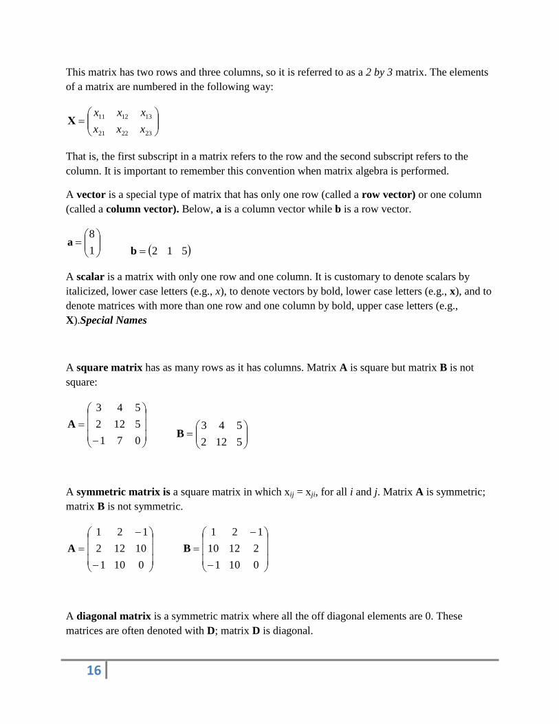
This matrix has two rows and three columns, so it is referred to as a 2 by 3 matrix. The elements

of a matrix are numbered in the following way:

232221

131211

xxx

xxxΧ

That is, the first subscript in a matrix refers to the row and the second subscript refers to the

column. It is important to remember this convention when matrix algebra is performed.

A vector is a special type of matrix that has only one row (called a row vector) or one column

(called a column vector). Below, a is a column vector while b is a row vector.

1

8a

512b

A scalar is a matrix with only one row and one column. It is customary to denote scalars by

italicized, lower case letters (e.g., x), to denote vectors by bold, lower case letters (e.g., x), and to

denote matrices with more than one row and one column by bold, upper case letters (e.g.,

X).Special Names

A square matrix has as many rows as it has columns. Matrix A is square but matrix B is not

square:

071

5122

543

A

5122

543B

A symmetric matrix is a square matrix in which xij = xji, for all i and j. Matrix A is symmetric;

matrix B is not symmetric.

0101

10122

121

A

0101

21210

121

B

A diagonal matrix is a symmetric matrix where all the off diagonal elements are 0. These

matrices are often denoted with D; matrix D is diagonal.

FOR FULLNOTES CALL/TEXT:0724 962 47717

700

020

004

D

An identity matrix is a diagonal matrix with 1s and only 1s on the diagonal. The identity matrix

is almost always denoted as I.

100

010

001

I

Matrix Algebra

Addition and Subtraction

To add two matrices, they both must have the same number of rows and they both must have the

same number of columns. The elements of the two matrices are simply added together, element

by element, to produce the results. That is, for R = A + B, then rij = aij + bij.

040

521

1010

061

5103

911

0101

10122

121

Matrix subtraction works in the same way, except that elements are subtracted instead of added.

Matrix Multiplication

There are several rules for matrix multiplication. The first concerns the multiplication between a

matrix and a scalar. Here, each element in the product matrix is simply the scalar multiplied by

the element in the matrix. That is, for R = aB, then rij = abij for all i and j. Thus,

2412

812

63

234

18 August 2015

Matrix multiplication involving a scalar is commutative. That is, aB = Ba. The next rule involves

the multiplication of a row vector by a column vector. To perform this, the row vector must have

as many columns as the column vector has rows.

For example,

2

1

0

210

is legal.

But,

2

0411

is not legal because the row vector has three columns while the column

vector has two rows.

The product of a row vector multiplied by a column vector will be a scalar. This scalar is simply

the sum of the first row vector element multiplied by the first column vector element plus the

second row vector element multiplied by the second column vector element plus the product of

the third elements, etc. In algebra, if r = ab, then

n

i

iibar1 . Thus,

52*21*10*0

2

1

0

210

All other types of matrix multiplication involve the multiplication of a row vector and a column

vector. Specifically, in the expression R = AB, jiijr ba where ia

the ith

row vector in matrix A

and jbis the j

th column vector in matrix B. Thus, if

120

151A

17

40

21

B

then

87*10*51*1

7

0

1

1511111

bar

and

FOR FULLNOTES CALL/TEXT:0724 962 47719

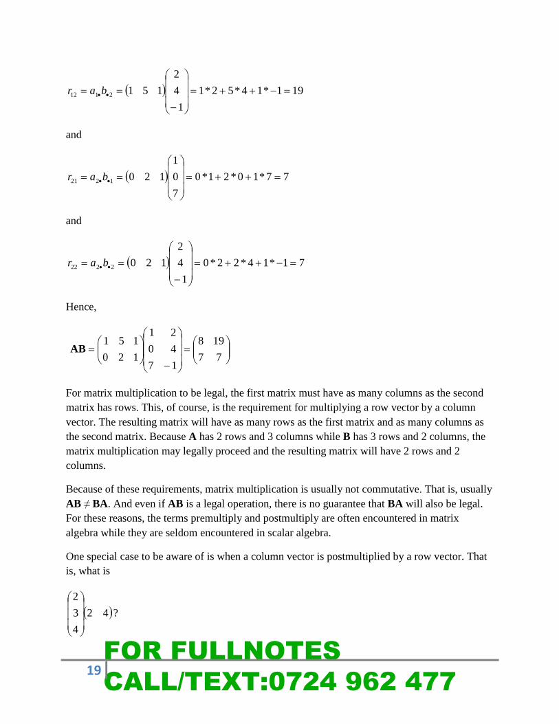
191*14*52*1

1

4

2

1512112

bar

and

77*10*21*0

7

0

1

1201221

bar

and

71*14*22*0

1

4

2

1202222

bar

Hence,

77

198

17

40

21

120

151AB

For matrix multiplication to be legal, the first matrix must have as many columns as the second

matrix has rows. This, of course, is the requirement for multiplying a row vector by a column

vector. The resulting matrix will have as many rows as the first matrix and as many columns as

the second matrix. Because A has 2 rows and 3 columns while B has 3 rows and 2 columns, the

matrix multiplication may legally proceed and the resulting matrix will have 2 rows and 2

columns.

Because of these requirements, matrix multiplication is usually not commutative. That is, usually

AB ≠ BA. And even if AB is a legal operation, there is no guarantee that BA will also be legal.

For these reasons, the terms premultiply and postmultiply are often encountered in matrix

algebra while they are seldom encountered in scalar algebra.

One special case to be aware of is when a column vector is postmultiplied by a row vector. That

is, what is

?42

4

3

2

20

In this case, one simply follows the rules given above for the multiplication of two matrices.

Note that the first matrix has one column and the second matrix has one row, so the matrix

multiplication is legal. The resulting matrix will have as many rows as the first matrix (3) and as

many columns as the second matrix (2). Hence, the result is

168

126

84

42

4

3

2

Similarly, multiplication of a matrix times a vector (or a vector times a matrix) will also conform

to the multiplication of two matrices. For example,

4

3

2

168

126

84

is an illegal operation because the number of columns in the first matrix (2) does not match the

number of rows in the second matrix (3). However,

8

6

4

0*161*8

0*121*6

0*81*4

0

1

168

126

84

and

19313*35*27*07*35*23*0

37

55

73

320

The last special case of matrix multiplication involves the identity matrix, I. The identity matrix

operates as the number 1 does in scalar algebra. That is, any vector or matrix multiplied by an

identity matrix is simply the original vector or matrix. Hence, aI = a, IX = X, etc. Note,

however, that a scalar multiplied by an identify matrix becomes a diagonal matrix with the

scalars on the diagonal. That is,

20

02

10

012

and not 2. This should be verified by reviewing the rules for multiplying a scalar and a matrix

given above.

FOR FULLNOTES CALL/TEXT:0724 962 47721

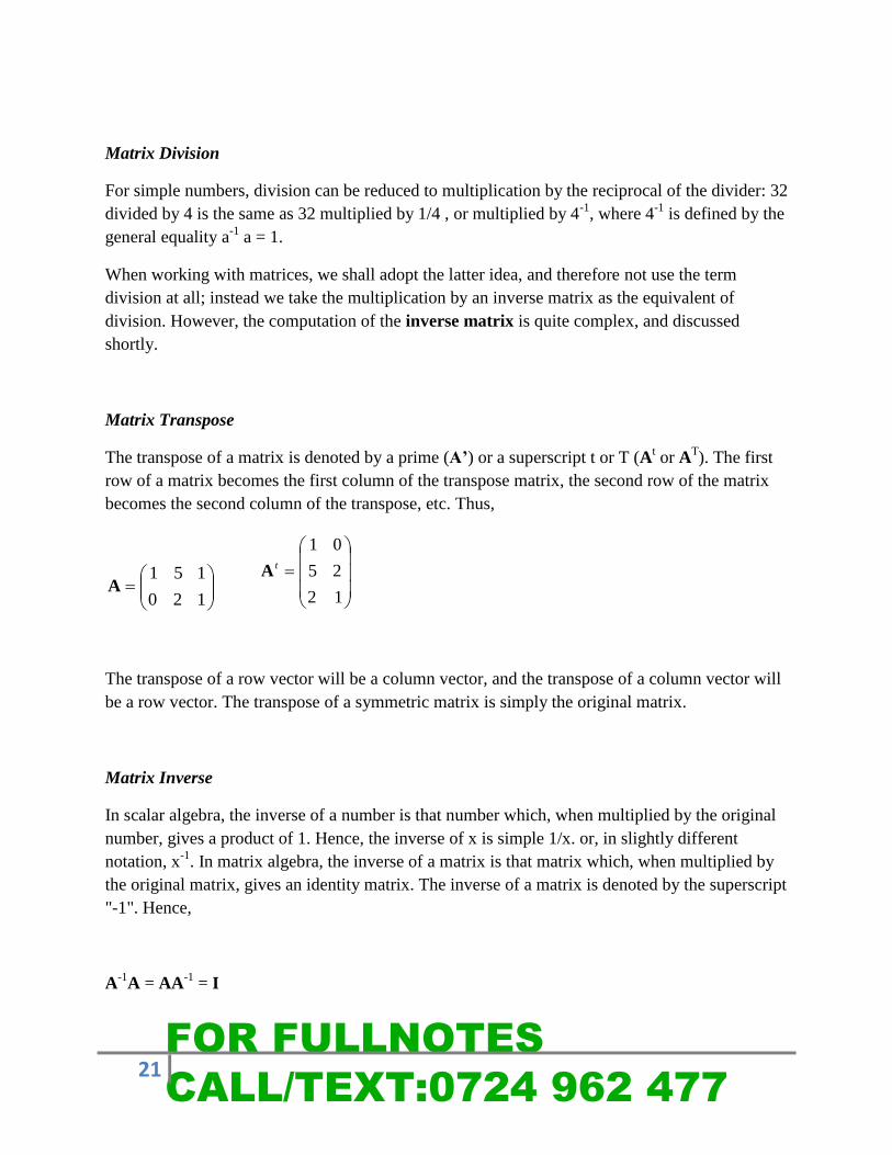
Matrix Division

For simple numbers, division can be reduced to multiplication by the reciprocal of the divider: 32

divided by 4 is the same as 32 multiplied by 1/4 , or multiplied by 4-1

, where 4-1

is defined by the

general equality a-1

a = 1.

When working with matrices, we shall adopt the latter idea, and therefore not use the term

division at all; instead we take the multiplication by an inverse matrix as the equivalent of

division. However, the computation of the inverse matrix is quite complex, and discussed

shortly.

Matrix Transpose

The transpose of a matrix is denoted by a prime (A’) or a superscript t or T (At or A

T). The first

row of a matrix becomes the first column of the transpose matrix, the second row of the matrix

becomes the second column of the transpose, etc. Thus,

120

151A

12

25

01t

A

The transpose of a row vector will be a column vector, and the transpose of a column vector will

be a row vector. The transpose of a symmetric matrix is simply the original matrix.

Matrix Inverse

In scalar algebra, the inverse of a number is that number which, when multiplied by the original

number, gives a product of 1. Hence, the inverse of x is simple 1/x. or, in slightly different

notation, x-1

. In matrix algebra, the inverse of a matrix is that matrix which, when multiplied by

the original matrix, gives an identity matrix. The inverse of a matrix is denoted by the superscript

"-1". Hence,

A-1

A = AA-1

= I

22

A matrix must be square to have an inverse, but not all square matrices have an inverse. In some

cases, when the determinant of the matrix is zero, the inverse does not exist. For covariance and

correlation matrices, an inverse will always exist, provided that there are more subjects than

there are variables and that every variable has a variance greater than 0.

It is important to know what an inverse is in multivariate statistics, but it is not necessary to

know how to compute an inverse. There are several ways to compute the inverse. The general

way is by solving a set of structural equations in which the elements of the inverse matrix are the

unknowns. A simple way to compute the inverse, involves the transpose, but this only works

when the column vectors are orthogonal, that is when x•1 • x•2 = 0. When

2221

1211

xx

xxA

is orthogonal, then 1

1

0

2

22

2

21

2

12

2

11

22211211

xx

xx

xxxx

will hold.

When matrix A is transposed we obtain At.

2212

2111

xx

xxt

A

When we compute At A we obtain:

IAA

10

012

22

2

2122211211

22211211

2

12

2

11

2212

2111

2221

1211

xxxxxx

xxxxxx

xx

xx

xx

xxt

Therefore, when A orthogonal, then At is A

-1.

The inverse of a product of two matrices is the swapped product of the individual inverse

matrices. Thus: (AB)-1

= B-1

A-1

. Where it is assumed that A and B are square and that A-1

and

B-1

exist. The proof is straightforward. Let AB be given, then we have

(AB) (AB)-1

= (AB) (B-1

A-1

) = A (B B-1

) A-1

= A I A-1

= A A-1

= I.

Determinant of a Matrix

The determinant of a matrix is a scalar and is denoted as |A| or det(A). The determinant is a

value. It has very important mathematical properties, but it is very difficult to provide a

substantive definition. It requires some steps to show how the value is found.

FOR FULLNOTES CALL/TEXT:0724 962 47723

If A is of order n x n, then the determinant is said to be or order n. Given a determinant |A| of

order n, we can form products of n elements in such a way that from each row and column of |A|

one and only one element is selected as a factor for the product. This is more easily seen in an

example. Suppose |A| is of third order:

333231

232221

131211

xxx

xxx

xxx

A

then 333231

232221

131211

xxx

xxx

xxx

A

Then the product x12x23x31 would satisfy the requirement: we have x12 as the only element form

the first row (second column), x23 as the only element from the second row (third column), and

x31 as the only element form the third row (first column). Such a product is called a term of the

determinant

However, we can form many terms like this. Other examples are x12x21x33, x13x22x31. The

complete set appears to be:

x11x22x33, x11x32x23

x12x21x33, x12x23x31

x13x21x32, x13x22x31

Note that there is systematicity in this. Start with the first row and than multiply with the left and

right diagonal elements of the submatrices. Or more formal, because we have one element out of

each row, we can always rank the elements in each term in such a way the row indices follow

the natural numbers. All that is left is to determine an order for the second subscripts; clearly

they can be taken in as many ways as there are permutations, we can form 3! = 6 terms for a

determinant of order 3. In general, a determinant of order n will have n! terms.

The next step is to assign a plus or a minus sign to each term. Assuming again that the row

subscripts are in natural order, the sign depends on the column subscripts only. First we shall

agree that every time a higher subscript precedes a lower, we have an inversion. Looking back at

the terms just presented, we have 0, 1, 1, 2, 2, and 3 inversions. For terms with an odd number of

inversions, the sign becomes negative.

It is now possible to compute the determinant of A.

|A| = x11x22x33 - x11x32x23 - x12x21x33 + x12x23x31 + x13x21x32 - x13x22x31

24

A numerical example:

The following rules are important for, and can help you sometimes:

1. The determinant of A has the same value as the determinant of A‘.

2. The value of the determinant changes sign if one row (column) is interchanged with

another row (column).

3. If a determinant has two equal rows (columns), its value is zero.

4. If a determinant has two rows (columns) with proportional elements, its value is zero.

5. If all elements in a row (column) are multiplied by a constant, the value of the

determinant is multiplied by that constant.

6. If a determinant has a row (column) in which all elements are zero, the value of the

determinant is zero.

7. The value of the determinant remains unchanged if one row (column) is added to or

subtracted form another row (column). Moreover, if a row (column) is multiplied by a

constant and then added to or subtracted from another row (column) the value remains

unchanged.

For covariance and correlation matrices, the determinant is a number that is sometimes used to

express the "generalized variance" of the matrix. That is, covariance matrices with small

determinants denote variables that are redundant or highly correlated (this is something that is

used in factor analysis, or regression analysis). Matrices with large determinants denote variables

that are independent of one another. The determinant has several very important properties for

some multivariate stats (e.g., change in R2 in multiple regression can be expressed as a ratio of

determinants). It is obvious that the computation of the determinant is a tedious business, so only

fools calculate the determinant of a large matrix by hand. We will try to avoid that, and have the

computer do it for us.

Illustration 1: Jane Mary and Joseph purchased cereals A, Band C from Faida super market. Jane purchased 1kg of A, 3kg of B and C and spent a total of ksh.650 on each Mary purchased 1kg, 4kg and 2kg of A, B, C and spent ksh.700. Joseph bought 2kg of A&B and 1kg of C and spent 650

I. Express the following information in a matrix form

II. Determine unit price of each type of cereals

FOR FULLNOTES CALL/TEXT:0724 962 47725

solution

Let X -Jane Y -mary Z -joseph

𝐴 + 3𝐵 + 3𝐶𝐴 + 4𝐵 + 2𝐶2𝐴 + 2𝐵 + 𝐶

= 650700650

|

1 + 3 + 31 + 4 + 22 + 2 + 1

𝐴𝐵𝐶 =

650700650

𝐷𝑒𝑡 = 1(4𝑥1 − 2𝑥2) − 3(1𝑥1 − 2𝑥2) + 3(1𝑥2 − 2𝑥4)

𝐷𝑒𝑡 = (1𝑥0) − (3𝑥3) + (3𝑥 − 6)

= 0 + 9 − 18

= −9

Inverse method

To find an inverse of a matrix, find

Determinant

Minor

Co-factor

Adjoint

Divide adjoint with determinant

0 −3 −6−3 −5 −4−6 −1 1

Row 2 (3x1)-(2x3)= -3

(1x1)-(2x3)= -5

(1x2)-(2x3)= -4

Row 3 (3x2)-(4x3)= -6

(1x2)-(1x3)= -1

(1x4)-(1x3)= -1

Cofactor

26

+ − +− + −+ − +

0 3 63 −5 4−6 1 1

Adjoint

0 3 63 −5 4−6 1 1

1

−9

𝐴− = A x AT

𝐴− =

0 −39

63

−39

59

−19

69

−49

−19

𝐴𝐵𝐶 =

0 −39

63

−39

59

−19

69

−49

−19

650700650

𝐴𝐵𝐶 =

0x650 −39 x700 6

3 x650

−39 x650 5

9 x700 −19 x650

69 x650 −4

9 x700 −19 x650

𝐴𝐵𝐶 =

20010050

FOR FULLNOTES CALL/TEXT:0724 962 47727

CRAMMER’S METHOD

A:

𝒉𝟏 𝑏 𝑐𝒉𝟐 𝑒 𝑓𝒉𝟑 𝑕 𝑖

𝑎 𝑏 𝑐𝑑 𝑒 𝑓𝑔 𝑕 𝑖

= 𝑋1

650 3 3700 4 2650 2 1

−9= 𝐴

Numerator 650 4𝑥1 − (2𝑥2) − 3 700𝑥1 − (650𝑥3) + 3 700𝑥2 − (650𝑥4)

= −1800

𝐴 =−1800

−9

𝐴 = 200

B:

𝑎 𝒉𝟏 𝑐𝑑 𝒉𝟐 𝑓𝑔 𝒉𝟑 𝑖

𝑎 𝑏 𝑐𝑑 𝑒 𝑓𝑔 𝑕 𝑖

= 𝑋2

1 650 31 700 22 650 1

−9= 𝐵

𝐵 =−900

−9

𝐵 = 100 C:

28

1 3 6501 4 7002 2 650

−9= 𝐶

𝐶 =−450

−9

𝐶 = 100 REDUCTION METHOD

FOR FULLNOTES CALL/TEXT:0724 962 47729

Illustration 2: Mary is employed as a sales lady in a company she is paid a basic salary and a commission on sales paid. Mary is paid a commission of sh.x on additional sales made above sh.100,000. During the month of July, august and September 2004: Mary made the sales and gross earnings as shown:

Months Sales Gross earning

July 300 000 23 000

August 200 000 20 000

September 50 000 14 750

In September 2004, she had 2weeks sick leave thus sales were low. a) Rates and commission applied.

b) Basic salary

c) Gross earnings of October 2004 when she made sales worth sh.400, 000.

Solution:

a) Rates and commission applied.

=100 000

100𝑥1000𝑥

30

Application of equation or functions in cost-volume-profit analysis

It can be applied in the following areas:

a) Demand function (price function)

THIS IS A FREE SAMPLE OF THE ACTUAL NOTES TO GET FULL/COMPLETE

NOTES:

Call/Text/Whatsapp:0724 962 477

You can also write to us at: 24sevenstudy@gmail.com

To download more resources visit: http://www.mykasnebnotes.com

For updates and insights like us on Facebook

STUDY NOTES|REVISION KITS|PILOT PAPERS|COURSE OUTLINE|STUDY TIPS|