Paper No. 6146 - Ohio

ADVANCEMENT IN PREDICTIVE MODELING OF MILD STEEL CORROSION IN CO₂ AND H₂S CONTAINING ENVIRONMENTS

Srdjan Nesic, Yougui Zheng, Bruce Brown, Jing Ning Institute for Corrosion and Multiphase Technology

Department of Chemical and Biomolecular Engineering Ohio University 342 W. State St.

Athens, OH 45701

ABSTRACT

Over the past decade, the knowledge related to predicting internal pipeline corrosion for sweet and particularly sour environments has dramatically improved. Advancement in understanding of the corrosion mechanisms related to H₂S corrosion environments enabled the development of an integrated electrochemical model for CO2/H₂S uniform corrosion, including the effect of H₂S on the protective corrosion product formation on mild steel.

The latest model of uniform CO₂/H₂S corrosion of carbon steel accounts for the key processes underlying of corrosion: chemical reactions in the bulk solution, electrochemical reactions at the steel surface, the mass transport between the bulk solution to the steel surface, and the corrosion product formation and growth (iron carbonate and iron sulfide). The model is able to predict the corrosion rate as well as the surface water chemistry as related to all the key species involved. The model has been successfully calibrated against experimental data in conditions where corrosion product layer do not form and in environments where they do, and compared to other similar models.

Key words: carbon dioxide, hydrogen sulfide, corrosion model.

INTRODUCTION Corrosion predictive models are a very useful tool that can be used to determine corrosion allowances, make predictions of facilities remaining life, and provide guidance in corrosion management. When it comes to internal corrosion of mild steel in the oil and gas industry, the mechanism of CO₂ corrosion is well understood through laboratory investigations.1,2 Hence, models for CO₂ corrosion developed in the past, range from those based on empirical correlations to mechanistic models describing the different processes involved in CO₂ corrosion of carbon steel. In 2002, Nyborg3 published a performance-based review of several CO₂ corrosion models focusing on the ability to account for effects of pH, protective iron carbonate layers, oil wetting, fluid flow, H₂S, top-of-the line corrosion, and acetic acid. Some five

1

Paper No.

6146

©2015 by NACE International. Requests for permission to publish this manuscript in any form, in part or in whole, must be in writing to NACE International, Publications Division, 15835 Park Ten Place, Houston, Texas 77084. The material presented and the views expressed in this paper are solely those of the author(s) and are not necessarily endorsed by the Association.

years later, Nesic published a comprehensive review of the understanding and modeling practices for internal corrosion of oil and gas pipelines.4 In the case of H₂S corrosion, there are numerous experimental studies; however, the mechanism of H₂S corrosion is still unclear and only a few models have been developed and published in the open literature for pure H₂S or mixed CO₂/H₂S corrosion. It has been widely observed that the uniform corrosion rate is reduced in the presence of very small concentrations of H₂S (1 mbar or even smaller) at room temperature and higher. To account for this effect one approach is to use a factor related to H₂S concentration and correct the predicted sweet (CO₂) corrosion rate. For example, Anderko, et al.,5 (1999) developed a mechanistic model to predict the corrosion rates of carbon steel in both CO₂ and H₂S containing environments, which includes a thermodynamic calculation to predict corrosion product composition and an electrochemical corrosion model to simulate the processes of cathodic and anodic reactions on the steel surface. To get the desired performance, the predictions of the electrochemical model were simply correlated to the final steady state corrosion rate experimental data, by using a surface coverage factor of iron sulfide and iron carbonate. Mechanistic verification of this approach using electrochemical kinetics data was not performed, and the water chemistry at the steel surface and in the bulk solution was not distinguished in their model. Sun and Nesic2,6, (2009) published a mechanistic corrosion model based on an assumption that in the presence of H₂S the corrosion rate is always mass transfer control due to the ubiquitous presence of iron sulfide layers. This model was calibrated with a wide range of experimental results and was found to be a useful tool for the prediction of transient corrosion rates arising from the growth of iron sulfide layers. However, the model consists of a number of assumptions which were not explicitly verified. In particular, it was universally assumed that the rate of corrosion in the presence of H2S is always under mass transfer control, hence the electrochemical reactions were not defined nor included in the model. This made it harder to integrate this model with mechanistic (electrochemical) models of CO2 corrosion.

Almost a decade ago, at the NACE 2006 conference, Nesic and Pots7 presented an overview of the state-of-the art in modeling of internal corrosion of oil and gas pipelines made from carbon steel which covered various mathematical modeling strategies, their strengths and their weaknesses. The present paper is an update of that overview, with a strong focus on modeling of the effects of H₂S and mixed CO₂/H₂S uniform corrosion,

PHYSICOCHEMICAL PROCESSES UNDELYING CO₂/H₂S CORROSION CO₂/H₂S corrosion is a complex process involving multiple physicochemical processes occurring simultaneously. These are: chemical reactions in the bulk solution, mass transport of aqueous species through the liquid boundary layer and the porous surface layer, electrochemical reactions at the steel surface and porous corrosion product layer formation which may or may not be protective. All these processes must be taken into account in a predictive model to provide a realistic estimation of the corrosion rate. For CO₂ corrosion, a electrochemical mechanistic model8,9 based on the key physicochemical processes has been developed and implemented into a software package which is well known and freely available.10,11 For H₂S corrosion, Sun and Nesic’s mass transfer model6 was also publically available and widely implemented.2,10,11 Based on the recent experimental findings, and the more thorough understanding that has emerged in the meantime, a more comprehensive uniform aqueous H₂S corrosion model can now be formulated and is described below.

We can start the outline of the new physicochemical model by picturing aqueous H₂S diffusing to a steel surface where it reacts rapidly to form a very thin adsorbed sulfide layer, as suggested by Marcus, et al.12 Following the mechanism proposed by Smith and Wright13, we can write:

2


𝐅𝐞(𝐬) + 𝐇𝟐𝐒(𝐚𝐪) → 𝐅𝐞𝐒(𝐚𝐝) + 𝟐𝐇(𝐚𝐝) (1)

The work of Marcus et al.12 indicates that sulfur adsorbs very strongly to a steel surface and can displace adsorbed H2O and OH-. This action results in slowing down the kinetics of electrochemical reactions such Fe dissolution, H₂O reduction, and carbonic acid reduction, apparently by affecting the double layer. The electrochemical reactions (both anodic and cathodic) continue to go forward despite an existing adsorbed sulfide layer, albeit at a slower rate.

When the surface concentrations of Fe²⁺ and S²⁻ ions exceed the solubility limit of iron sulfide (initially mackinawite), solid iron sulfide is thermodynamically stable, and it will precipitate on the steel surface:

𝐅𝐞(𝐚𝐪)𝟐+ + 𝐒(𝐚𝐪)

𝟐− ⇔ 𝐅𝐞𝐒(𝐬) (2)

This iron sulfide layer can grow and retard the corrosion rate via a surface coverage effect and a mass transfer effect (acting as diffusion barrier). The present transient corrosion model is somewhat similar, but also quite different from the model proposed by Sun and Nesic6 in some key elements. A comparison between the key differences for the two models is listed in Table 1.

Table 1 Differences between Sun-Nesic model6 and the present model

Sun-Nesic model (2009)6 Present model

A thin inner mackinawite film formed by direct chemical reaction acting as a solid state diffusion barrier.

A thin adsorbed iron sulfide film affecting directly the kinetics of different electrochemical reactions (retardation effect).

A porous outer iron sulfide layer formed by spalling of the inner layer.

A porous outer iron sulfide layer formed via a precipitation mechanism.

Corrosion rate is always under mass-transfer control due to the porous outer iron sulfide layer and inner mackinawite film.

Corrosion rate is not always under mass-transfer control depending the kinetics of mass transfer and electrochemical reactions.

MODEL DESCRIPTION The present model describes H₂S/CO₂ corrosion in terms of two main processes: an electrochemical corrosion process including effect of mass transport from bulk to the surface, and corrosion product formation and growth process for iron carbonate and iron sulfide.

Electrochemical Corrosion Model The concentration of the species can be very different in the bulk solution and at the corroding steel surface due to corrosion, mass transfer effects and chemical reactions. One usually knows (or can readily calculate) the bulk species concentration, however, the electrochemical corrosion process depends on the surface concentrations. Therefore the surface concentrations need to be estimated by calculation. In the present model, two calculation “nodes” were used in the computational domain: one for the species concentrations in the bulk solution and the other for the species concentrations in the thin water layer adjacent to the corroding steel surface. The concentrations of chemical species in the

3


bulk solution can be calculated using a standard water chemistry equilibrium model. The concentrations of species at the corroding steel surface need to be calculated in a way that ensures that all the key physicochemical processes that affect the surface concentrations are accounted for (see Figure 1). These are:

1. Homogenous chemical reactions close to the steel surface.

2. Electrochemical reactions at the steel surface.

3. Transport of species between the steel surface and the bulk, including convection and diffusion through the boundary layer as well as electromigration due to establishment of electrical potential gradients.

These three physicochemical processes are interconnected and can be expressed by writing a material balance or mass conservation equation for a thin surface water layer.

jjwje R

xNN

tc

+∆

−=

∂

∂ ,,jsurface, (3)

where jsurface,c is the concentration of species j, jeN , is the flux of species j on the east boundary due to

mass transfer from the bulk solution to the surface, jwN , is the flux of species j on the east boundary due to electrochemical reactions at the steel surface, and jR is the source/sink term due to homogeneous chemical reactions involving species j.

Figure 1: Illustration of computation domain and governing equations for mass transport

simulation.

Homogenous Chemical Reactions

The homogenous reactions considered in the present model are well known and readily available in the open literature.1,2,8 The reactions describe the interaction between various species (H₂S, HS⁻, S2-, CO₂, H₂CO₃, HCO₃⁻, CO₃²⁻, OH⁻, and H⁺).

4


It should be noted that chemical reactions are often very rapid when compared to other processes involved in corrosion, such as species transport and electrochemical reactions, thus preserving chemical equilibria throughout the solution. On the other hand, in the case of slow chemical reactions (such as the CO2 hydration reaction), other faster processes can lead to local non-equilibrium conditions at the corroding steel surface. Therefore, chemical reactions can significantly affect the rates of electrochemical processes at the steel surface and the ultimately – the corrosion rate.

In order to better understand how the rates of homogenous chemical reactions are calculated in the present model, one is referred to the papers by Nešić, et al.1,2,8

Electrochemical Reactions at the Steel Surface Electrochemical reactions at the steel surface considered in the present model include:

Fe(s) → Fe(aq)2+ + 2e− (4)

2H (aq)+ + 2e− → H2(g) (5)

2H2CO3(aq) + 2e− → H2(g) + HCO3−

(aq) (6)

H2S(aq) + 2e− → H2(g) + 2HS(aq)−

(7)

2H2O(l) + 2e− → H2(g) + OH(𝑎𝑞)− (8)

The Tafel equation used to calculate the current densities (rate) of various electrochemical reactions listed above is described in detail in the previously published paper on the electrochemical corrosion model14,15:

𝑖 = 𝑖𝑜 10±𝐸−𝐸𝑜𝑏 (9)

where 𝑖 represents the reaction current density in A/m2, 𝑖𝑜 represents a reference current density in A/m2 , 𝐸 represents the corrosion potential of the steel in V, 𝐸𝑜 represents a reference potential in V, and 𝑏 represents the Tafel slope in V/decade. In this model, the current density for each electrochemical reaction depends on the surface concentration of species, which is not explicitly known and needs to be calculated, as explained below. For a spontaneous corrosion process, the unknown corrosion potential of the steel, E can be calculated from the charge balance equation at the steel surface:

� 𝑖𝑐𝑎𝑡ℎ𝑜𝑑𝑖𝑐

= � 𝑖𝑎𝑛𝑜𝑑𝑖𝑐

(10)

5


Details of this calculation have already been explained elsewhere14,15. Then the flux at the steel surface can be determined from:

𝑁𝑤,𝑗 = ±𝑖𝑗

𝑛𝑗𝐹

(11)

where 𝑛𝑗 is the number of moles of electrons exchanged per mol of species j participating in a particular electrochemical reaction. For species j consumed by electrochemical reactions at the steel surface, the positive sign is applied. For species j produced by electrochemical reactions at the steel surface, the negative sign is applied. For those species j that are not involved in the electrochemical reactions, 𝑖𝑗 = 0. Once the corrosion potential (E) is found, the partial current (𝑖𝑗) for a given species j is readily calculated from Equation (9).

Species Surface Concentration and Mass Transfer Ten minor species (H₂S, HS⁻, S2-, CO₂, H₂CO₃, HCO₃⁻, CO₃²⁻, OH⁻, H⁺, and Fe²⁺) and two major species (Na+ and Cl-) were accounted for by calculating their mass transfer flux between the bulk solution and the steel surface. The terms “major” and “minor” refer to the magnitude of species concentration, with Na+ and Cl- exceeding the concentration of other species by orders of magnitude. It should be noted that the concentrations of species are not calculated throughout the mass transfer boundary layer, as is done in more advanced models presented by Nesic’s et al.8,9 due to inherent complexities associated with this approach. Rather, only two calcuation nodes are used, one in the bulk and the other at the steel surface, so the mass transfer flux between the bulk solution to the steel surface can be calculated for each of the species using a mass transfer coefficient, 𝑘𝑚,𝑗 approach:

𝑁𝑒,𝑗 = 𝑘𝑚,𝑗 �𝑐𝑏𝑢𝑙𝑘, 𝑗 − 𝑐𝑠𝑢𝑟𝑓𝑎𝑐𝑒,𝑗� + 𝑘𝑚,𝑗 𝑧𝑗𝐹𝑅𝑇

𝑐𝑏𝑢𝑙𝑘,𝑗∆Φ (12)

Here 𝑐𝑏𝑢𝑙𝑘, 𝑗 is the concentration of the species j in the bulk solution, 𝑐𝑠𝑢𝑟𝑓𝑎𝑐𝑒,𝑗 is the concentration of the species j at the steel surface, 𝑧𝑗 is the electric charge of species j. The mass transfer coefficient of species j, 𝑘𝑚,𝑗, can be calculated from well-known correlations such as the one for a rotating cylinder electrode (RCE) proposed by Eisenberg16:

𝑆ℎ = 0.0791 𝑅𝑒0.7 𝑆𝑐0.356 (13)

or for turbulent single phase pipe flow the mass transfer coefficient can be calculated by a straight pipe correlation of Berger and Hau:17

𝑆ℎ = 0.0165 𝑅𝑒0.86 𝑆𝑐0.33 (14)

6


The last term, ∆Φ, in the transport equation (11) represents electromigration due to a small electrical potential difference between the bulk solution and the surface water layer, which is significant only for the transport of major species (Na+ and Cl-).

Substitution of flux density due to electrochemical reactions and mass transfer processes into mass conservation equation of Equation (3) yields the final transport equation which can be written for each species:

∆𝑥 𝜕𝐶𝑠𝑢𝑟𝑓𝑎𝑐𝑒,𝑗

𝜕𝑡= − 𝑖𝑗

𝑛𝑗𝐹+ 𝑘𝑚,𝑗 �𝑐𝑏𝑢𝑙𝑘,𝑗 − 𝑐𝑠𝑢𝑟𝑓𝑎𝑐𝑒,𝑗� + 𝑘𝑚,𝑗 𝑧𝑗𝐹

𝑅𝑇𝑐𝑏𝑢𝑙𝑘,𝑗∆Φ + ∆𝑥 ∗ 𝑅𝑗 (15)

There are 13 unknowns (12 unknown surface concentrations and the potential gradient, ∆Φ), and only 12 transport equations. Since the aqueous solution is always charge neutral, the electroneutrality equation must be satisfied:

� 𝑧𝑗𝑐𝑠𝑢𝑟𝑓𝑎𝑐𝑒,𝑗 = 0 (16)

The concentration for all the considered chemical species at the steel surface can now be calculated by solving these 13 equations. At the same time, the corrosion current and the corrosion potential are calculated using Equations (9) and Equation (10).

Model of Corrosion Product Layer Growth From the electrochemical corrosion model described in the previous section, the surface water chemistry (the concentration of different chemical species at the steel surface) and the corrosion potential of the steel are obtained. Using this information, a thermodynamic model can be used to predict which solid corrosion product may form on the steel surface (solubility calculation).18,19 If this calculation suggests that solubility of a given salt is not exceeded, the corrosion process at the bare steel surface proceeds unimpeded. If any given solubility is exceeded, a corrosion product layer forms on the steel surface. The formation of the corrosion product layer may significantly affect the corrosion process. Therefore, a corrosion product layer growth model, which focuses on kinetics of iron sulfide and iron carbonate formation, was developed to address this issue.

In the corrosion model described above, two nodes were considered in the computational domain for species concentration calculation: one in the bulk solution and the other at the steel surface. When a corrosion product layer forms, one more node needs to be added to account for this, as shown in Figure 2.

7


Figure 2: Sketch of corrosion process with corrosion product layer.

Formation of an iron sulfide and/or iron carbonate corrosion product layer affects the fluxes and thereby the concentrations of species at the steel surface, that in turn changes the kinetics of the electrochemical processes and corrosion. To reflect this, the mass conservation equation, Equation (3), needs to be slightly modified to read:

jjwjejsurface R

xNN

tc

+∆

−=

∂∂ ,,,ε

(17)

here, ε is the porosity of the corrosion product layer. The rate of reaction jR (source or sink of species j) now includes both homogeneous chemical reactions and heterogeneous chemical reactions such as iron sulfide and/or iron carbonate precipitation. The flux of species between the bulk and the steel surface jeN , is also different as it is affected by the diffusion through the porous corrosion product layer.

The flux of species due to electrochemical reactions at the steel surface jwN , is also changed due to the partial coverage of the surface by the corrosion product layer. How these three terms, jR , jeN , and

jwN , are calculated exactly, when a corrosion product layer forms, is addressed below.

Heterogeneous Chemical Reactions Homogenous reactions have been discussed in the previous section. The focus here is on two new heterogeneous chemical reactions: iron carbonate and iron sulfide formation.

Iron Carbonate Formation

Iron carbonate forms when the product of the concentrations of Fe2+ and CO32- ions exceeds the

solubility limit according to:

Fe(aq)2+ + CO3(aq)

2− → FeCO3(s) (18)

8


This reaction acts as a sink for Fe2+ and CO32- species, and the kinetics can be calculated using

Equation (19) proposed by Sun, et al. 20:

𝑅𝐹𝑒𝐶𝑂3(𝑠) = 𝑒28.20 − 64.85𝑅𝑇

𝑆𝑉

𝐾𝑠𝑝𝐹𝑒𝐶𝑂3�𝑆𝐹𝑒𝐶𝑂3 − 1� (19)

where 𝑅𝐹𝑒𝐶𝑂3(𝑠) is the precipitation rate in mol/(m3 s); 𝑆𝑉

is the surface to volume ratio of the iron carbonate in 1/m; 𝑆𝐹𝑒𝐶𝑂3 is the saturation value of iron carbonate (considering only super saturation, i.e. when 𝑆𝐹𝑒𝐶𝑂3 >1), and 𝐾𝑠𝑝𝐹𝑒𝐶𝑂3 is the solubility limit of iron carbonate in (mol/L)2, which is given by Equation (20)20 .

𝑙𝑜𝑔𝐾𝑠𝑝𝐹𝑒𝐶𝑂3 = −59.3498 − 0.041377 𝑇 −2.1963

𝑇+ 24.5724 𝑙𝑜𝑔𝑇 + 2.518𝐼0.5 − 0.657 𝐼 (20)

where T is the temperature in K and I is the ionic strength in mol/L.

Iron Sulfide Formation

The iron sulfide layer forms when the product of the concentrations of Fe2+ and S2- ions exceeds the solubility limit according to:

Fe(aq)2+ + S(aq)

2− → FeS(s) (21)

The precipitation kinetics are much faster for iron sulfide than for iron carbonate and the solubility limit is lower. Therefore, in the present model, when an iron sulfide layer can precipitate (SFeS>1), iron carbonate precipitation is not considered. Although some previous researchers21,22 have addressed the precipitation kinetics of iron sulfide, a reliable expression for the precipitation kinetics is still elusive. A new expression is suggested here, which is similar in essence to the one for iron carbonate precipitation kinetics:

𝑅𝐹𝑒𝑆(𝑠) = 𝑒48 − 40,000𝑅𝑇 𝑆

𝑉 𝐾𝑠𝑝,𝑆2− (𝑆𝐹𝑒𝑆 − 1) (22)

In this expression, the constants were calibrated with the experimental results from the present study (shown below) and by using Harmandas et al.21 The saturation value for iron sulfide is denoted by 𝑆𝐹𝑒𝑆 and 𝐾𝑠𝑝,𝑆2− is the solubility limit of iron sulfide in (mol/L)2, which can be calculated from Benning et al.23:

9


𝐾𝑠𝑝,𝑆2− = 102848.779

𝑇 − 6.347 𝐾ℎ𝑠 𝐾𝑏𝑠 (23)

Here, Khs and Kbs are the equilibrium constants for the H₂S first dissociation and second dissociation, which are obtained from the open literature.24,25

Effect of Corrosion Product layer on Electrochemical Reactions The electrochemical reactions are mainly affected by the surface coverage effect where the corrosion product layer makes parts of the steel surface unavailable for corrosion. Assuming the surface coverage is equal to the volumetric porosity of the corrosion product layer, the current density of each electrochemical reaction (9) now becomes:

𝑖 = 𝜀 𝑖𝑜 10±𝐸−𝐸𝑜𝑏 (24)

Based on the change in the current density, the flux jeN , at the steel surface can be calculated using Equation (11). The rate of the electrochemical reactions is also affected by the changes in surface concentrations of various species due to retarded mass transfer through the porous corrosion product layer, as described below.

Effect of Porous Corrosion Product Layer on Mass Transfer The governing equations used to quantify the mass transfer process through the corrosion product layer for different species are similar to those described by Nesic et al.(2003).8 The retardation of mass transfer depends primarily on the properties of the corrosion product layer, such as the thickness, porosity and tortuosity. Considering the models available in the open literature, the mass transfer coefficient 𝑘𝑠,𝑗 of species j through the porous corrosion product layer is a function of the diffusion coefficient (Dj), porosity (ε), tortuosity (τ) and thickness (𝛿𝑠) of the corrosion product layer.26–29

𝑘𝑠,𝑗 =𝜀𝜏𝐷𝑗

𝛿𝑠 (25)

The tortuosity (𝜏) is taken to be proportional to the square root of porosity, in an analogy with the theory of porous electrodes.30 The total mass transfer coefficient from the bulk solution to the steel surface is represented by kT,j, which is the function of km,j and ks,j :

1𝑘𝑇,𝑗

=1

𝑘𝑠,𝑗+

1𝑘𝑚,𝑗 (26)

The corrosion product layer thickness ∆𝛿𝑠 change over time is calculated as follows:

- when iron sulfide layer forms:

10


∆𝛿𝑠 =Δ𝑥𝑅𝐹𝑒𝑆(𝑠)𝑀𝐹𝑒𝑆∆𝑡

𝜌𝐹𝑒𝑆(1 − ε) (27)

- when iron carbonate layer forms:

∆𝛿𝑠 =Δ𝑥𝑅𝐹𝑒𝐶𝑂3(𝑠)𝑀𝐹𝑒𝐶𝑂3∆𝑡

𝜌𝐹𝑒𝐶𝑂3(1 − ε) (28)

Here 𝑀𝐹𝑒𝑆 and 𝑀𝐹𝑒𝐶𝑂3 represent the molecular weight of iron sulfide and iron carbonate (kg/mol); Δ𝑡 is the time step; 𝜌𝐹𝑒𝑆 and 𝜌𝐹𝑒𝐶𝑂3 are the density of iron sulfide and iron carbonate (kg/m3).

The change in surface corrosion layer porosity ε is calculated explicitly using a corrosion product layer growth model developed by Nesic et al. ,9 as shown by mass balance equations Equation (29) and Equation (30). The detailed derivation of these equations is explained in the original paper and will not be repeated here.

- for the iron carbonate layer:

xCRR

Mt FeCO

FeCO

FeCO

∂∂

−−=∂∂ ε

ρε

3

3

3 (29)

- for the iron sulfide layer:

xCRRM

t FeSFeS

FeS

∂∂

−−=∂∂ ε

ρε (30)

At the interface between corrosion product layer and steel surface, ε is taken to be 1, as the corrosion process continuously creates voids underneath the corrosion product layer. The initial porosity was also set as 1.

The procedure for the calculation of the corrosion rate over time is sought at discrete time steps. First, the initial corrosion rate, including surface water chemistry, is determined by the electrochemical corrosion model without the effect of any corrosion product layer. Then, a corrosion product prediction model based on thermodynamic framework is used to determine whether a corrosion product layer forms or not on the steel surface. If a corrosion product layer doesn’t form, the calculation is over and a bare steel corrosion rate is the result. If a corrosion product layer does form, a corrosion product layer growth model is invoked. The change in porosity for the corrosion product layer is calculated from Equation (29) or (30), and the change in thickness of layer growth is obtained from Equation (27) or

11


Equation (28) depending on which corrosion products forms. Finally, the mass conservation equations for each species are solved. Therefore, the concentration for all the chemical species at the steel surface can be obtained. The corrosion current, corrosion potential, corrosion rate, potential gradient in solution and the rates (currents) for each of the cathodic reactions and the anodic reaction are calculated.

MODEL VERIFICATION Although the present model was primarily developed to address H₂S corrosion and combined H₂S/ CO₂ corrosion, it also has the capability of predicting pure CO₂ corrosion. Since the entire mathematical model was revised and simplified, this new model needs to be compared with other models and verified with experimental data.

Verification of Corrosion Model without Corrosion Product Layer Comparisons with Other Models

The comparison was done with two other advanced multi-node models, i.e., model presented by Nesic’s et al. 8,9 (denoted as Model Nesic) and a corrosion model developed by Pots (denoted as Model Pots)31.

For a pure CO₂ environment, the predicted corrosion rate, surface pH and CO32- concentration at 25 °C

from these different models are shown in Figure 3. Reasonably good agreement is obtained. Many other comparisons were made for various conditions and it was concluded that the present model is directly comparable in performance with the other two models, while being much simpler than either of them.

Figure 3: Comparison between the present model and two other models (Model Nesic and Model

Pots) for a pure CO₂ environment using velocities up to 8 m/s at 25 °C, [Fe2+ ]=1 ppm, pH 4.0, 1bar CO₂, pipeline diameter = 0.1 m, 1 wt% NaCl.

Comparisons with Experimental Results

A model cannot be used with confidence before its performance is compared with experimental results. Various comparisons with laboratory data are presented below. Figure 4 shows the comparisons between the present model and experimental data for an aqueous acidic environment purged by N₂ (without any CO₂ or H₂S) at pH 4.0 and various flow velocities. The predictions made by Model Nesic are also added to the plots, in order to get a better sense how this well-established model is comparing with the same experimental data. One can conclude that for a pure acidic environment the predictions

12


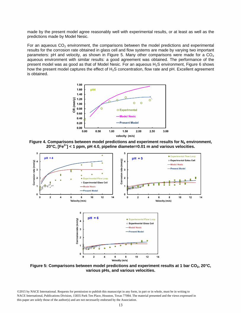
made by the present model agree reasonably well with experimental results, or at least as well as the predictions made by Model Nesic.

For an aqueous CO₂ environment, the comparisons between the model predictions and experimental results for the corrosion rate obtained in glass cell and flow systems are made by varying two important parameters: pH and velocity, as shown in Figure 5. Many other comparisons were made for a CO₂ aqueous environment with similar results: a good agreement was obtained. The performance of the present model was as good as that of Model Nesic. For an aqueous H₂S environment, Figure 6 shows how the present model captures the effect of H₂S concentration, flow rate and pH. Excellent agreement is obtained.

Figure 4. Comparisons between model predictions and experiment results for N₂ environment,

20°C, [Fe2+] < 1 ppm, pH 4.0, pipeline diameter=0.01 m and various velocities.

Figure 5: Comparisons between model predictions and experiment results at 1 bar CO₂, 20°C,

various pHs, and various velocities.

13


Figure 6: Comparisons between model predictions and experiment results for 30°C, 1 bar total

pressure and various H₂S concentrations, velocities and pHs. Verification of Corrosion Model for Conditions when Iron Carbonate Corrosion Layer Forms Figure 7 shows the comparisons of the model predictions with results of experiments conducted in a CO2 aqueous solution under flowing conditions, for conditions when protective iron carbonate corrosion product layer forms. The corrosion rate was rapidly reduced, however, these experiments are notoriously difficult to reproduce, as indicated by differences in results from five repeats of a nominally identical experiment. The model predictions are within the range of the variation of experimental data, and are similar to those made by Model Nesic. This indicates that the present model is capable of simulating the iron carbonate layer growth kinetics and the effect on the CO2 corrosion rate.

Figure 7: Comparisons between the model predictions and the experiment results for iron carbonate layer forming condition at pH 6.6, 80°C, 0.53 bar CO₂, and 1000rpm rotating speed, 50

ppm bulk Fe2+.

14


Verification of Corrosion Model for Conditions when Iron Sulfide Layer Forms Effect of pH2S

The partial pressure of H₂S, is directly relates to the aqueous H₂S concentration in the solution, and is an important factor as it plays dual and oposing roles. First, aqueous H₂S is a corrosive species accelerating the corrosion rate by enhancing the cathodic reaction rate. Second, H₂S also promotes the rate of the iron sulfide precipitation that decreases the general corrosion rate. Figure 8 illustrates the predicted effect of pH₂S on the corrosion rate calculated by the present model. The initial corrosion rate increases with increasing pH₂S, because no corrosion product layer protectiveness is accounted for at the initial time (time zero), the system is overwhelmed by the accelerating role of H₂S reduction. However, during longer reaction times, such as 1 day, the formation of a protective iron sulfide layer is promoted by pH₂S. The best example of the dual roles of H₂S is that at 10 bar pH₂S, the initial corrosion rate is the highest, but the corrosion rate after 1 day is the lowest.

Figure 8. The predicted effect of pH₂S on the corrosion rate from present model for pH 5.0,

T=80oC, V=1 m/s. The model by Sun-Nesic6 of H2S corrosion was a precursor of the current work, as described above. Both models: the Model Sun-Nesic and the present model were compared with the experimental data, as shown below. First, the performance at low partial pressures of H₂S was examined. The test was conducted by Sun6 at H₂S gas partial pressures from 0.54 mbar to 54 mbar. Figure 9 shows that both the present model and Model Sun-Nesic capture the corrosion rate change well.

Figure 9. Corrosion rate changing with time at different H₂S partial pressure from present model

and Model Sun-Nesic; points: experimental data, lines: model predictions; conditions: total pressure = 1 bar, H₂S gas partial pressure from 0.54 mbar to 54 mbar, 80°C, experiment duration

1 h to 24 h, pH 5.0 to 5.5, stagnant. Experimental data taken from Sun 6.

15


Corrosion experiments at higher pH₂S (pH₂S= 16.1 bar in the mixed H₂S/N₂ environment) were reported by Liu et al.32 and model predictions are compared with the experimental results in Figure 10. The present model performs much better than Model Sun-Nesic at this condition.

A similar range of H₂S partial pressures were reported by Bich, et al. 33 with the main difference being the presence of CO₂. Figure 11 shows the comparison between the model prediction and experimental results in a mixed H₂S/CO₂ environment. The present model captures the corrosion rate change with time, but Model Sun-Nesic tends to over predict the corrosion rate.

Figure 10. Corrosion rate changing with time, points: experimental data, lines: model

predictions; conditions: 16.1 bar H₂S, 90°C, 2L autoclave, stagnant. Experimental data taken from Liu, et al. 32

.

Figure 11. Corrosion rate changing with time, points: experimental data, lines: model

predictions; conditions: 12.2 bar H₂S, 3.5 bar CO₂, 65°C. Experimental data taken from Bich et al. 33

Effect of pH

The predicted effect of a change in pH on the corrosion rate for a pure H₂S environment when protective iron sulfide layer forms is demonstrated in Figure 12 and compared with experimental data.

16


Corrosion rate increases with a decrease in pH as expected, since the corrosivity of the solution increases and the solubility of iron increases as well. The decrease of corrosion rate with time is much faster at pH 6.0 due to the formation of a denser iron sulfide layer. The present model captures the corrosion rate change much better than Model Sun-Nesic. It is worth noting that the experimental LPR corrosion rates are much higher than the model prediction at pH 4.0. This is probably due to the iron carbide remaining on the metal surface from corrosion at pH 4.0, which can accelerate the corrosion rate by providing a more cathodic reaction area34,35. This effect is not included in the present model.

Figure 12: Corrosion rate changing with time, points: experimental data, lines: model

predictions; conditions: 0.054 bar pH2S, balance nitrogen, T = 80oC, stirring rate: 600 rpm.

Effect of Flow Fluid flow and turbulence play an important role in the corrosion process. Higher flow can increase the corrosion rate through enhancing the mass transport process, especially when there is no corrosion product layer formed. Flow can also affect the formation of a protective iron sulfide layer. Species transport in turbulent flow affects the surface concentration of species and, consequently, changes the precipitation rate of iron sulfide. Figure 13 shows the comparisons between model predictions and experimental results at different flow conditions. The present model is generally able to predict the change of the corrosion rate rather well.

Figure 13: Corrosion rate vs. time, points: experimental data, lines: model predictions;

conditions: pH₂S = 0.054 bar, balance nitrogen, T=80 oC, pH 5.0.

17


Effect of Temperature Increasing temperature makes the bare steel corrosion rate higher as seen in the beginning of the experiments shown in Figure 14 and Figure 15. However, the formation of a protective iron sulfide layer is also promoted at high temperature, and therefore, the corrosion rate decreases more rapidly with temperature increase. Comparisons between model prediction and experimental results at different temperatures, shown in Figure 14 and Figure 15 faithfully capture this behavior. The predictions of the effect of temperature on corrosion rate are better than those made by Model Sun-Nesic.


conditions: total pressure=1 bar, pH₂S = 0.1 bar at 25 °C, pH₂S = 0.054 bar at 80 oC, pH 6.0, 400 rpm stirring rate. Experimental data taken from Ning36


conditions: total pressure= 1 bar, pH₂S=0.3 bar at 90 °C, pH₂S=0.88 bar at 50 °C pH 4.2-4.7, Stirring condition. Experimental data taken from Abayarathna, et al.37

CONCLUSIONS A relatively simple mechanistic transient model of uniform CO₂/H₂S corrosion of carbon steel has been developed, which accounts for the key processes underlying corrosion:

o chemical reactions in the bulk solution, o electrochemical reactions at the steel surface, o mass transport between the bulk solution to the steel surface, and o corrosion product formation and growth (iron carbonate and iron sulfide).

18


The model is able to predict the corrosion rate as well as the surface concentration of all key species involved in the corrosion process. The model has been successfully calibrated against experimental data in conditions where corrosion product layer do not form and in those where they do. Parametric testing of the model in iron sulfide forming conditions has been done in order to gain insight into the effect of various environmental parameters on the H₂S/CO₂ corrosion process. Performance of the present model was favorably compared to the performance of other similar models which are publically available.

REFERENCES 1. S. Nešić, “Carbon Dioxide Corrosion of Mild Steel,” in Uhligs Corrosion. Handbook, 3rd edition,

edited by R.W. Revie,(John Wiley & Sons, Inc., 2011), pp. 229–245. 2. S. Nesic and W. Sun, “Corrosion in Acid Gas Solutions,” Sheir’s Corrosion, 2nd edition, editied by

J.A. Richardson et al., (Elsevier, 2010), pp. 1270–1298. 3. R. Nyborg, “Overview of CO2 Corrosion Models for Wells and Pipelines,” CORROSION/2002,

paper no. 02233 (Houston, TX: NACE, 2002). 4. S. Nesic, “Key Issues Related to Modelling of Internal Corrosion of Oil and Gas Pipelines: A

Review,” Corros. Sci. 49 (2007): pp. 4308–4338. 5. A. Anderko, P. McKenzie, and R. D. Young, “Computation of Rates of General Corrosion Using

Electrochemical and Thermodynamic Models,” Corrosion 57 (2001): pp. 202–213. 6. W. Sun and S. Nesic, “A Mechanistic Model of Uniform Hydrogen Sulfide/carbon Dioxide

Corrosion of Mild Steel,” Corrosion 65 (2009): pp. 291–307. 7. S. Nesic and B. F. M. Pots, “Predictive Modeling in CO2 and H2S Containing Environments,”

CORROSION/2006, paper no.06116 (Houston TX: NACE, 2006). 8. S. Nesic, A. Stangeland, M. Nordsveen, and R. Nyborg, “A Mechanistic Model for Carbon Dioxide

Corrosion of Mild Steel in the Presence of Protective Iron Carbonate Films Part 2: A Numerical Experiment,” Corrosion 59 (2003): pp. 489–497.

9. S. Nesic and K. L. J. Lee, “A Mechanistic Model for Carbon Dioxide Corrosion of Mild Steel in the Presence of Protective Iron Carbonate Films Part 3: Film Growth Model,” Corrosion 59 (2003): pp. 616–628.

10. S. Nesic, H. Li, J. Huang, and D. Sormaz, “An Open Source Mechanistic Model for CO2 / H2S Corrosion of Carbon Steel,” CORROSION/2009, paper no. 09572 (Houston TX: NACE, 2009).

11. “FREECORP - Corrosion Prediction Software”, Ohio University, http://www.corrosioncenter.ohiou.edu/software/freecorp/.

12. P. Marcus and E. Protopopoff, “Potential-pH Diagrams for Adsorbed Species: Application to Sulfur Adsorbed on Iron in Water at 25 °C and 300 °C,” J. Electrochem. Soc. 137 (1990): pp. 2709–2712.

13. S. N. Smith and E. J. Wright, “Prediction of Minimum H2S Levels Required for Slightly Sour Corrosion,” Corrosion/94, paper no. 11 (Houston TX: NACE, 1994).

14. Y. Zheng, B. Brown, and S. Nešić, “Electrochemical Study and Modeling of H2S Corrosion of Mild Steel,” Corrosion 70 (2014): pp. 351–365.

15. Y. Zheng, J. Ning, B. Brown, and S. Nesic, “Electrochemical Model of Mild Steel Corrosion in a Mixed H2S/CO2 Aqueous Environment,” CORROSION/2014, paper no. 3907 (Houston, TX: NACE, 2014).

16. M. Eisenberg, C. W. Tobias, and C. R. Wilke, “Ionic Mass Transfer and Concentration Polarization at Rotating Electrodes,” J. Electrochem. Soc. 101 (1954): pp. 306–320.

17. F. P. Berger and K.-F. F.-L. Hau, “Mass Transfer in Turbulent Pipe Flow Measured by the Electrochemical Method,” Int. J. Heat Mass Transf. 20 (1977): pp. 1185–1194.

18. J. Ning, Y. Zheng, D. Young, B. Brown, and S. Nešić, “Thermodynamic Study of Hydrogen Sulfide Corrosion of Mild Steel,” Corrosion 70 (2014): pp. 375–389.

19


19. T. Tanupabrungsun, “Thermodynamics and Kinetics of Carbon Dioxide Corrosion of Mild Steel at Elevated Temperatures,” Ph.D. dissertation, Ohio University, 2012.

20. W. Sun, “Kinetics of Iron Carbonate and Iron Sulfide Scale Formation in Carbon Dioxide/hydrogen Sulfide Corrosion,” Ph.D. dissertation, Ohio University, 2006.

21. N. G. Harmandas and P. G. Koutsoukos, “The Formation of iron(II) Sulfides in Aqueous Solutions,” J. Cryst. Growth 167 (1996): pp. 719–724.

22. D. Rickard, “Kinetics of FeS Precipitation: Part 1. Competing Reaction Mechanisms,” Geochim. Cosmochim. Acta 59 (1995): pp. 4367–4379.

23. L. G. Benning, R. T. Wilkin, and H. L. Barnes, “Reaction Pathways in the FeS System below 100 °C,” Chem. Geol. 167 (2000): pp. 25–51.

24. O. M. Suleimenov and R. E. Krupp, “Solubility of Hydrogen Sulfide in Pure Water and in NaCl Solutions, from 20 to 320 °C and at Saturation Pressures,” Geochim. Cosmochim. Acta 58 (1994): pp. 2433–2444.

25. Y. K. Kharaka, W. D. Gunter, P. K. Aggarwal, E. H. Perkins, and J. D. Dedraal, “SOLMINEQ. 88: A Computer Program for Geochemical Modeling of Water - Rock Interactions” (Menlo Park, CA: Alberta Research Council, 1988).

26. E. L. Cussler, Diffusion: Mass Transfer in Fluid Systems, 2nd edition (Cambridge, UK: Cambridge University Press, 1997).

27. P. Grathwohl, Diffusion in Natural Porous Media: Contaminant Transport, Sorption/desorption and Dissolution Kinetics (New York, NY: Springer US, 1998).

28. M. Gopal, S. Rajappa, and R. Zhang, “Modeling the Diffusion Effects through the Iron Carbonate Layer in the Carbon Dioxide Corrosion of Carbon Steel,” CORROSION/98, paper no. 98026 (Houston TX: NACE, 1998).

29. D. Mu, Z.-S. Liu, C. Huang, and N. Djilali, “Determination of the Effective Diffusion Coefficient in Porous Media Including Knudsen Effects,” Microfluid. Nanofluidics 4 (2008): pp. 257–260.

30. L. Pisani, “Simple Expression for the Tortuosity of Porous Media,” Transp. Porous Media 88 (2011): pp. 193–203.

31. B. F. M. Pots, “Mechanistic Models for the Prediction of CO2 Corrosion Rates under Multi-Phase Flow Conditions,” CORROSION/95, paper no. 137 (Houston, TX: NACE, 1995).

32. M. Liu, J. Wang, W. Ke, and E.-H. Han, “Corrosion Behavior of X52 Anti-H2S Pipeline Steel Exposed to High H2S Concentration Solutions at 90 °C,” J. Mater. Sci. Technol. 30 (2014): pp. 504–510.

33. N. N. Bich and K. G. Goerz, “Caroline Pipeline Failure: Findings on Corrosion Mechanisms in Wet Sour Gas Systems Containing Significant CO2,” CORROSION/96, paper no. 96026 (Houston, TX: NACE, 1996).

34. F. Farelas, B. Brown, and S. Nesic, “Iron Carbide and Its Influence on the Formation of Protective Iron Carbonate in CO2 Corrosion of Mild Steel,” CORROSION/2013, paper no. 02291 (Houston TX: NACE, 2013).

35. T. Berntsen, M. Seiersten, and T. Hemmingsen, “Effect of FeCO3 Supersaturation and Carbide Exposure on the CO2 Corrosion Rate of Carbon Steel,” Corrosion 69 (2013): pp. 601–613.

36. J. Ning, “Investigation of Polymorphous Iron Sulfide in H2S Corrosion of Mild Steel,” Ohio University Advisory Board Meeting (Ohio University, 2013).

37. D. Abayarathna, A. R. Naraghi, and S. Wang, “The Effect of Surface Films on Corrosion of Carbon Steel in a CO2-H2S-H2O System,” CORROSION/2005, paper no. 08417 (Houston, TX: NACE, 2005).

20


Documents

Paper No. 6146 - Ohio