Embed Size (px)
Citation preview

1
Paper 3370-2015
PROC RANK, PROC SQL, PROC FORMAT and PROC GMAP Team Up and a (Map) Legend is Born!
Christianna Williams, PhD, Chapel Hill, NC Louise Hadden, Abt Associates Inc., Cambridge, MA
ABSTRACT
The task was to produce a figure legend that gave the quintile ranges of a continuous measure corresponding to each color on a five-color choropleth US map. Actually, we needed to produce the figures and associated legends for several dozen maps for several dozen different continuous measures and time periods as well as associated "alt-text" for compliance with Section 508…so, the process needed to be automated. A method was devised using SAS
® PROC RANK to generate the quintiles, PROC SQL to get
the data value ranges within each quintile, and PROC FORMAT (with the CNTLIN= option) to generate and store the legend labels. The resulting data files and format catalogs are then used to generate both the maps (with legends) and associated "alt text". Then, these processes were rolled into a macro to apply the method for the many different maps and their legends. Each part of the method is quite simple – even mundane – but together these techniques allowed us to standardize and automate an otherwise very tedious process. The same basic strategy could be used whenever one needs to dynamically generate data "buckets" but then keep track of the bucket boundaries – whether for producing labels, map legends, "alt-text", or so that future data can be benchmarked against the stored categories.
xx Figure 3.16a. Percentage of Nursing Home Residents Taking Antipsychotic Medication, 2011 xx
Source: MDS; measures are fully described in the Methods section
Numbers in parentheses in legend indicate number of states in a given category
Figure 1. Example figure with legend indicating range for each of the five colors and number of states in that category.

2
INTRODUCTION
One of our ongoing projects is to help in the annual production of a lengthy report published by the Centers for Medicare and Medicaid Services (CMS) called the Nursing Home Data Compendium (CMS, 2014). This roughly 150-page book presents descriptive summary information in the form of tables, figures and maps on all Medicare- and Medicaid-certified nursing homes in the US and the residents in these facilities. Data on nursing home characteristics (such as occupancy levels), health inspection results (such as the average number of and severity of citations for violations to health regulations) and resident characteristics (such as the percent of residents taking antipsychotic medications or reporting severe pain) are presented in summary form, generally broken down by provider characteristics that are of interest to CMS and researchers, such as for-profit vs. not-for-profit nursing homes or by state. Of course, an effective way to present geographic (in this case state-to-state) variation in some measure of interest is with a map, and the Nursing Home Data Compendium includes a lot of US maps – specifically five-color chloropleth maps (sometimes called “heat maps”), in which each state is presented in one of five colors, corresponding to quintiles of the measure being mapped. An example of such a map is shown in Figure 1.
The purpose of this paper is to describe in detail how both the figure and the figure legends are produced. The figure legends were an interesting problem, because they differ for each map, based on the range and distribution of the measure being mapped (e.g. percent of residents taking antipsychotic medications as shown in Figure 1). Also, note that the legend includes the number of states in each of the five groups,
1 and we describe how that information is added to the legend data. The paper also describes the
production of “alt-text”, which allows the final product to be used with screen readers and refreshable Braille displays making figures compliant with Section 508, a federal law requiring that federal agencies make electronic and information technology accessible to people with disabilities, including low vision. While the basic process is very straightforward, there were a few interesting wrinkles in making the process reproducible, and in “macro-tizing” the code. Also, because there were two programmers and MANY figures involved, we wanted to standardize the process, data structure and naming conventions to facilitate efficient, consistent and reproducible production. An earlier version of this paper (Williams, 2014) described the production of the figure legend, but not the figure itself or the “alt-text.” Some other coding challenges involved with producing the Nursing Home Data Compendium have also been described (Hadden, 2014).
OVERVIEW OF THE PROCESS
The basic steps in the process are shown here. The remainder of the paper will describe each of these steps and provide the associated code.
1) Summarize individual-level data to state level, rounding to the desired degree of precision. 2) Use PROC RANK to generate quintiles. 3) Use PROC SQL to obtain the upper and lower bounds of each quintile and the number of states
in each range. 4) Prepare the input data set for PROC FORMAT with a DATA step. 5) Use PROC FORMAT to add FORMAT that maps the quintile value to the legend labels to a
format library. 6) Generate a permanent data set containing all the information needed to produce the figure and
the legend. 7) Use PROC GMAP to produce a map and legend from this data. 8) Use DATA Step code and PROC REPORT to generate “alt” text describing the map for Section
508 compliance, using the same input data as the map and legend.
1 While the number of states in each quintile should be around 10, it does vary slightly due to rounding and because Washington,
DC is included (so N=51 “states” for each map. Additionally, we keep the same “bin” thresholds for some longitudinal presentations (e.g. a separate map for 3 successive years), and in this case, if there is a secular trend in the data, the number of states in each “quintile” may vary substantially from one year to the next.

3
Steps 2 through 8 are repeated for each measure (map). After the code was working as desired for a single measure, macros incorporating steps 2 through 6, and steps 7 and 8 were built that could simply be called once for each measure. The macro code is also included at the end of the paper.
STEP 1. SUMMARIZE DATA TO STATE LEVEL
All the measures of interest described in this paper begin as binary (i.e. yes/no) indicators at the level of the individual nursing home resident. A federally mandated assessment tool is administered to every resident of every Medicare- or Medicaid certified nursing home on admission and on a quarterly basis, and the indicators are derived from this assessment. The resident data we process are de-identified; however, they include a facility ID that can be linked to the state where the facility is located (as well as other basic facility characteristics such as size and profit status). In order to generate state prevalence estimates for the data compendium, we simply aggregate these 0/1 measures up to the state level. It is, of course, very handy that the mean of a 0/1 measure will give a prevalence at the desired level of aggregation. Though for many applications it may be desirable to process each measure separately, here it was efficient to summarize many measures at once. We used PROC SUMMARY, which is handy here because we can very easily just use the “MEAN=” option on the OUTPUT statement to assign the original variable names to the state averages, and these new variables retain the LABELs (if any, of the raw variables). The resulting data set has 51 observations, one for each state plus the District of Columbia. In the DATA step shown below we round each measure to the nearest thousandth (or tenth of one percent); this is enough precision to distinguish substantive differences among the states and will reduce confusion later about which quintile a state should go in.
* STEP 1: Summarize 0/1 resident indicators to state level;
PROC SUMMARY DATA = residents NWAY ;
CLASS state ;
VAR Age_ge65 Age_ge85 Age_ge95 Minority ADLimp0 ADLimp_ge4 Falls_any
Falls_inj_any Presulc Restrnt_any Incontinent FeedingTube WeightLoss
Antipsych;
OUTPUT OUT = statesum MEAN=;
RUN;
* Round before getting ranges;
DATA statesum_all ;
SET statesum (DROP = _:);
ARRAY unr{14} Age_ge65 Age_ge85 Age_ge95 Minority ADLimp0 ADLimp_ge4 Falls_any
Falls_inj_any Presulc Restrnt_any Incontinent FeedingTube WeightLoss
Antipsych;
ARRAY rnd{14} Age_ge65R Age_ge85R Age_ge95R MinorityR ADLimp0R ADLimp_ge4R
Falls_anyR Falls_inj_anyR PresulcR Restrnt_anyR IncontinentR FeedingTubeR
WeightLossR AntipsychR;
DO i = 1 TO 14;
RND{i} = ROUND(unr{i},0.001) ;
END;
DROP i;
RUN;
A partial print of the Statesum_All data set is shown in Output 1.
STATE PresUlc PresulcR Restrnt_any Restrnt_anyR Antipsych AntipsychR
AK 0.065292 0.065 0.008591 0.009 0.14433 0.144
AL 0.048739 0.049 0.012544 0.013 0.26161 0.262
AR 0.044360 0.044 0.020304 0.020 0.27412 0.274
AZ 0.059019 0.059 0.007005 0.007 0.21618 0.216
CA 0.063499 0.063 0.029076 0.029 0.23185 0.232
Output 1. Print selected summary data, rounded and unrounded for 5 states

4
STEP 2: USE PROC RANK TO GENERATE QUINTILES
For the next several steps, it is simplest to process one measure at a time. Here we provide the code for a single measure, and at the end of the paper provide the macros that get called once for each measure. The use of a consistent naming convention for the variables and the output data set that will simplify implementing a macro later as well as sharing the data among co-authors! PROC RANK with the GROUPS=5 option will assign each state to a quintile for each measure.
* STEP 2: Generate quintiles;
PROC RANK DATA = statesum_all GROUPS=5
OUT = stateranks_Antipsych (KEEP = state Antipsych:);
VAR AntipsychR;
RANKS Antipsych_5 ;
RUN;
A partial print of the StateRanks_Antipsych data set is shown in Output 2.
STATE Antipsych AntipsychR Antipsych_5
AK 0.14433 0.144 0
AL 0.26161 0.262 3
AR 0.27412 0.274 4
AZ 0.21618 0.216 1
CA 0.23185 0.232 2
Output 2. Print the StateRanks_Antipsych data set for 5 states
STEP 3: USE PROC SQL TO OBTAIN DATA FOR MAP LEGEND
While PROC RANK very conveniently assigns states to quintiles of the measure, it does not readily tell us what the cut-points or thresholds are between one quintile and the next. We need this information for two purposes. First, we want to put it into the legend on our map. Second, we want to be able to assign future data to categories (or “bins”) based on the same ranges; for example, in the next edition of the data compendium, we may want to use the same categories so that we could see which states have changed “quintiles”
2. We also want to know how many states are in each bin because we want to include that in
the legend as well. PROC SQL readily provides this information. We use the rank (quintile) variable as the GROUP BY variable to obtain the MIN and MAX of the prevalence for each level as well as the number in each bin. The COUNT(*) syntax counts the number of rows in each of the groups defined by GROUP BY.
* STEP 3: Get Data needed for map legend;
PROC SQL ;
CREATE TABLE range_Antipsych AS
SELECT Antipsych_5 AS bin
,COUNT(*) AS n_in_bin
,MIN(AntipsychR) AS minAntipsych
,MAX(AntipsychR) AS maxAntipsych
FROM stateranks_Antipsych
GROUP BY Antipsych_5
ORDER BY Antipsych_5;
QUIT;
The resulting data set (range_Antipsych) has just five observations (one per bin). Output 3 has a complete listing.
2 The implementation of this second purpose is beyond the scope of this paper, and it involves some additional wrinkles (e.g. what if
new data falls outside the range of the old data), but knowing we were going to want to do this later guided some of the decisions for the current purpose – generating the data for the figure legends.

5
min max
bin n_in_bin Antipsych Antipsych
0 10 0.123 0.203
1 10 0.210 0.217
2 11 0.219 0.233
3 10 0.236 0.267
4 10 0.269 0.331
Output 3. Ranges for quintiles for the Antipsychotic measure and number of states in each group
STEP 4. PREPARE THE RANGE AND COUNT DATA SET FOR PROC FORMAT
We want to construct a FORMAT library to store all the legend labels. There are a few things we need to do to get the rangeAntipsych data set ready to be used as my CNTLIN= data set with PROC FORMAT. The DATA step code is shown below. Here is what is going on:
a) The RETAIN statement assigns a format name (Antipsychf) and specifies that we will be creating a numeric format. PROC FORMAT expects these variables to have the names FMTNAME and TYPE. Though it is trivial for a 5-observation data set, this method is slightly more efficient than assignment statements.
b) The required START and END values (which specify the range for the values to be formatted) both get the value of the variable BIN (0 to 4).
c) Note in Output 3 that there are gaps between the end of one range and the beginning of the next
range. This wouldn’t look right on our legend, nor would it work correctly when new data (which might well have values falling in these gaps) gets filtered with this format. So, beginning with bin 1, we want the starting value for the bin to be 0.1 greater than the ending value for the previous bin. I use the LAG function to make this happen.
d) MINVAL will hold the lower bound of each range and MAXVAL the upper bound. We multiply by 100 and round to the nearest tenth so that the values will be in the format xx.x (like a percent, which is the way people are used to seeing prevalence estimates).
e) Here we assign the values to the required LABEL variable, using concatenation functions (CATS and CAT) to format them precisely as desired.
* STEP 4: Prepare data as input to PROC FORMAT;
DATA cntl_Antipsych (DROP = space bincount);
SET range_Antipsych ;
RETAIN FMTNAME 'Antipsychf' /* STEP a */
TYPE 'N' ;
START = bin; /* STEP b */
END = bin;
lmaxAntipsych = LAG(maxAntipsych); /* STEP c */
* numeric start and end points for each of the bins ; /* STEP d */
IF bin = 0 THEN minval = ROUND(100*minAntipsych,0.1);
ELSE minval = ROUND(100* lmaxAntipsych + 0.1,0.1);
maxval = ROUND(100*maxAntipsych,0.1) ;
* convert above to labels for legend, adding # of states; /* STEP e */
LENGTH bincount $4 LABEL $18 ;
space = ' ';
bincount = CATS('(',PUT(n_in_bin,2.),')');
LABEL = CAT(PUT(minval,4.1),' to ',PUT(maxval,4.1),space,space,bincount) ;
RUN;
The resulting data set (cntl_Antipsych) is listed in Output 4. The only variables that will be used by PROC FORMAT are FMTNAME, TYPE, START, END, and LABEL, but the others are shown for clarity.

6
Note how the ranges have been extended to eliminate gaps in between. (As an aside, if we were going to use this data to create a format to assign new data to bins, we would use MINVAL and MAXVAL as our START and END and BIN as our LABEL.)
l
m m m
i a a
n x x
A A A
n n n n
_ t t f t
i i i m i m m
n p p t s p i a l
_ s s n t t s n x a
b b y y a y a e y v v b
i i c c m p r n c a a e
n n h h e e t d h l l l
0 10 0.123 0.203 Antipsychf N 0 0 . 12.3 20.3 12.3 to 20.3 (10)
1 10 0.210 0.217 Antipsychf N 1 1 0.203 20.4 21.7 20.4 to 21.7 (10)
2 11 0.219 0.233 Antipsychf N 2 2 0.217 21.8 23.3 21.8 to 23.3 (11)
3 10 0.236 0.267 Antipsychf N 3 3 0.233 23.4 26.7 23.4 to 26.7 (10)
4 10 0.269 0.331 Antipsychf N 4 4 0.267 26.8 33.1 26.8 to 33.1 (10)
Output 4. CNTLIN data set for construction of FORMAT to assign legend labels.
STEP 5. ADD FORMAT MAPPING QUINTILE VALUES TO LEGEND LABELS TO LIBRARY
The next step is extremely straightforward – just use PROC FORMAT to read the CNTL dataset built in the last step to generate a FORMAT and add it to a format library specific to the annual data compendium. The PROC CATALOG step that allows us to give a description to the format (which will show up in the format catalog’s metadata) is a nice touch.
* STEP 5: Add format for this measure to format library;
PROC FORMAT LIBRARY = LIBRARY.Compendium2011Res CNTLIN=cntl_Antipsych ;
RUN;
PROC CATALOG CATALOG = LIBRARY.Compendium2011Res ;
MODIFY Antipsychf.FORMAT (DESCRIPTION = "Legend labels for map [Antipsych]") ;
CONTENTS ;
RUN ;
QUIT;
The CONTENTS statement off PROC CATALOG will produce the listing shown in Output 5. Obviously this will be more useful when the catalog contains a lot of formats.
Contents of Catalog LIBRARY.COMPENDIUM2011RES
# Name Type Create Date Modified Date Description
-------------------------------------------------------------------------------------
1 ANTIPSYCHF FORMAT 07/21/2014 07/21/2014 Legend labels for map [Antipsych]
Output 5. Metadata (output from PROC CATALOG) for the legend label format(s).

7
STEP 6. GENERATE DATA SET WITH DATA NEEDED FOR FIGURE, LEGEND & “ALT-TEXT”
We decided to produce a little data set for each map which summarized the data neatly for mapping and production of the alt-text code with relatively little need for additional manipulation. While a DATA step could certainly be used here, we chose PROC SQL primarily because it allows us to easily specify the order of the variables on the resulting data set, and (control-freaks that we are), we wanted this to be consistent. I am also linking the state-level data set to the bin-level data set to add in variables needed for the alt-text. For the maps, we need states identified by their FIPS code, and the STFIPS function translates the two-letter postal abbreviation into the FIPS code. Similarly, the STNAMEL function converts the postal abbreviation to the full name of the state (in title case). We use the format we created in the last step to associate the correct legend label with each state. Note the OPTIONS FMTSEARCH statement at the top – this may be critical to ensure that the correct version of the format is used, if, for example, the ranges and/or number of states in each category change from one year to the next. The quintile variable itself (Antipsych_5) is the value that is actually “mapped” for each state. We will use the number of states in each quintile (bincount) and the range of values for each quintile (binrange) in producing the alt-text.
* STEP 6. Write data for one map to permanent file;
* make sure to use the correct format library ;
OPTIONS FMTSEARCH = (library.Compendium2011Res);
PROC SQL;
CREATE TABLE out.Antipsych (LABEL = "Data for Map of % of Residents Taking
Antipsychotics [var=Antipsych]") AS
SELECT
a.state AS state_abbr LABEL = "State (postal abbreviation)"
, STFIPS(a.state) AS state_fips LABEL = "State (FIPS code)"
, STNAMEL(a.state) AS statename LABEL = "State Name"
, a.AntipsychR AS Antipsych LABEL = "% of Residents Taking
Antipsychotics (rounded)"
, a.Antipsych_5
LABEL = "Quintile for % of Residents Taking Antipsychotics [Antipsych]
(0=low,4=high)"
, PUT(a.Antipsych_5,Antipsychf.) AS legend_label
LABEL = "Range for Bin (# of States)"
, b.n_in_bin AS bincount
LABEL = 'Number of States in Quintile'
, CAT(PUT(b.minval,4.1),' to ',PUT(b.maxval,4.1)) AS binrange
LABEL = 'Text Range for Quintile (xx.x to yy.y)'
FROM stateranks_Antipsych a
INNER JOIN
cntl_Antipsych b
ON a.Antipsych_5 = b.bin
ORDER BY state ;
QUIT;
The resulting data set has one observation for each state (plus DC); a listing of the first several observations is shown in Output 6.
state_ state_ Antipsych_
abbr fips statename Antipsych 5 legend_label bincount binrange
AK 2 Alaska 0.144 0 12.3 to 20.3 (10) 10 12.3 to 20.3
AL 1 Alabama 0.262 3 23.4 to 26.7 (10) 10 23.4 to 26.7
AR 5 Arkansas 0.274 4 26.8 to 33.1 (10) 10 26.8 to 33.1
AZ 4 Arizona 0.216 1 20.4 to 21.7 (10) 10 20.4 to 21.7
CA 6 California 0.232 2 21.8 to 23.3 (11) 11 21.8 to 23.3
Output 6. Partial listing of final data set for mapping for one measure

8
STEP 7. GENERATE THE FIGURE & LEGEND
First, a “base” map data set which includes separate boxes for small states in the Northeast is created. All figures we generate are drawn using this map. The code for this map is loosely based on one of Robert Allison’s wonderful examples (Allison, 2012)
* STEP 7a. Generate base map w/ extra squares small Eastern states;
/* make the base map for all figures */
DATA mymap;
SET maps.us (WHERE=(state NE 72));
RUN;
/* create the extra 'square' for certain small states */
DATA extra_squares;
INPUT statecode $ 1-2;
state=STFIPS(statecode);
DATALINES;
NH
VT
MA
RI
CT
NJ
DE
MD
DC
;
RUN;
DATA extra_squares;
SET extra_squares;
RETAIN y;
segment=999;
IF _n_=1 THEN y=.14;
ELSE y=y-.010;
x=.345; OUTPUT; /* Each OUTPUT statement */
x=x+.025; OUTPUT; /* draws a line */
y=y-.020; OUTPUT;
x=x-.025; OUTPUT;
RUN;
DATA mymap;
SET mymap extra_squares;
state_name=FIPNAMEL(state);
RUN;
*labels with state code equidistant from bottom and top of square for each state;
PROC SQL;
CREATE TABLE extra_label AS
SELECT UNIQUE AVG(y) AS y
, AVG(x)+.02 AS x
, statecode AS text
FROM extra_squares
GROUP BY statecode;
QUIT;
***set annotate parameters to produce the labels;
DATA extra_label;
SET extra_label;
XSYS='2'; YSYS='2'; HSYS='3'; WHEN='a';
FUNCTION='label'; COLOR='gray55'; POSITION='6'; SIZE=2.25;
RUN;

9
As you will note in Output 6 above, the measure data set has a record for each state and the District of Columbia (Puerto Rico, the U.S. Virgin Islands and Territories are not included in the figures.) In order to generate the map legend, a summary data set with 5 records containing the categorized measure and legend level is required. This can be accomplished in a number of ways – among which is using the measure format in the format catalog along with PROC FORMAT with a CNTLOUT statement. We use a simple data step to create a macro variable for each of the legend labels.
*STEP 7b. Prepare legend labels for use in the map;
/* build macro variables for the labels */
PROC FREQ DATA=out.ANTIPSYCH;
TABLES ANTIPSYCH _5*legend_label / NOPRINT OUT=legend;
RUN;
DATA _NULL_;
LENGTH tvar $ 2;
SET legend;
tvar=CATS("T",PUT(antipsych_5 + 1, 1.));
CALL SYMPUT(tvar,legend_label) ;
RUN;
Input for the legend has one observation per legend label; a listing is shown in Output 7. After the CALL SYMPUT, there will be five macro variables &T1 - &T5, holding the respective legend labels.
Antipsych_5 legend_label COUNT PERCENT
0 12.3 to 20.3 (10) 10 19.6078
1 20.4 to 21.7 (10) 10 19.6078
2 21.8 to 23.3 (11) 11 21.5686
3 23.4 to 26.7 (10) 10 19.6078
4 26.8 to 33.1 (10) 10 19.6078
Output 7 Listing of a mini data set for the legend for one measure
In Step 7c, the map (with legend) is generated, with a file written to HTML as well as generating a PNG file. OPTIONS are set to output to a landscape page and suppress the printing of the date and page number; GOPTIONSs are set to determine the type of image (PNG), suppress a border around the graphic, determine the units used in measurements of the image, and assign text formatting; ODS listing is closed to suppress “windowing” of the graphic while running in batch, and ODS destination(s) (HTML) are selected. The result is in Figure 1.
*STEP 7c. Generate the map and legend, outputting to HTML (and a PNG file);
***Set options and parameters for output to create the map;
OPTIONS ORIENTATION=landscape NODATE NONUMBER;
GOPTIONS DEVICE=png NOBORDER;
ODS LISTING CLOSE;
ODS HTML PATH=odsout BODY="&invar._&year..htm" OPTIONS(pagebreak='no');
GOPTIONS cback=white;
GOPTIONS GUNIT=pct FTITLE="albany amt/bold" FTEXT="albany amt/bold";
GOPTIONS HTITLE=18pt HTEXT=11pt CTITLE=black CTEXT=gray55;
***create the legend using the macro variables for legend labels;
LEGEND1 LABEL=none ACROSS=5 CSHADOW=dodgerblue CFRAME=gold CBLOCK=dodgerblue
POSITION=(bottom center outside) SHAPE=bar(.15in,.15in) MODE=reserve
OFFSET=(0,0) VALUE=("&t1" "&t2" "&t3" "&t4" "&t5");
***set colors for the five values of measure_5;
PATTERN1 VALUE=msolid COLOR=white;
PATTERN2 VALUE=msolid COLOR=lightblue ;

10
PATTERN3 VALUE=msolid COLOR=CornflowerBlue ;
PATTERN4 VALUE=msolid COLOR=blue ;
PATTERN5 VALUE=msolid COLOR=navy;
***create some blank space at the top of the map;
TITLE1 a=-90 h=5pct " ";
TITLE2 a=90 h=1pct " ";
***add information to provide "hover text" when viewing the HTML file;
***The state name and measure percent appear when mousing over a state;
DATA my_data;
SET out.ANTIPSYCH (RENAME=(state_fips=state statename=state_name));
LENGTH my_html $100;
my_html='TITLE='||QUOTE(TRIM(LEFT(state_name))||': '||
TRIM(LEFT(PUT(&invar.*100,5.1))) );
RUN;
***generate the map using the annotate data set for extra squares;
PROC GMAP DATA=my_DATA MAP=mymap ALL ANNO=extra_label;
ID state_name;
CHORO antipsych_5 / DISCRETE COUTLINE=gold WOUTLINE=1
CDEFAULT=yellow
LEGEND=legend1
HTML=my_html
DES='' NAME="antipsych_2011 ";
RUN;
QUIT;
ODS _ALL_ CLOSE;
ODS LISTING;
STEP 8. GENERATE “ALT” TEXT FOR SECTION 508 COMPLIANCE
A combination of SAS procedures and data steps is used to manipulate the measure data set and create a paragraph describing the figure for each measure. An example of this paragraph is shown in Figure 2. The technique used features the ability to create very long variables with style information for formatting and line breaks, and reporting using PROC REPORT which allows very long variables to wrap.
Figure 3.16 . This is a five color map of the United States that displays the percentage of nursing home residents taking antipsychotic medication for each state. Ten states have 12.3 to 20.3 percent of nursing home residents taking antipsychotic medication including Alaska, Hawaii, Maryland, Michigan, Minnesota, North Carolina, Oregon, South Carolina, Wisconsin and Wyoming. Ten states have 20.4 to 21.7 percent of nursing home residents taking antipsychotic medication including Arizona, Colorado, Iowa, Montana, Nevada, New Jersey, North Dakota, Rhode Island, South Dakota and Washington. Eleven states have 21.8 to 23.3 percent of nursing home residents taking antipsychotic medication including California, Delaware, District of Columbia, Florida, Idaho, Indiana, New Mexico, New York, Pennsylvania, Virginia and West Virginia. Ten states have 23.4 to 26.7 percent of nursing home residents taking antipsychotic medication including Alabama, Connecticut, Georgia, Kentucky, Maine, Massachusetts, Nebraska, New Hampshire, Utah and Vermont. Ten states have 26.8 to 33.1 percent of nursing home residents taking antipsychotic medication including Arkansas, Illinois, Kansas, Louisiana, Mississippi, Missouri, Ohio, Oklahoma, Tennessee and Texas. Guam, Puerto Rico and the Virgin Islands are not included in this figure.
The source of data for this figure is the Minimum Data Set.
Figure 2. Example “alt” text to enable one figure to be compliant with Section 508

11
The first step (Step 8a) is to create a “bin” level data set from the state level data set. We use PROC SORT with the NODUPKEY option to accomplish this, keeping the variables needed for the “alt-text” description.
* STEP 8. Generate alt text for section 508 compliance;
***8a: create summary bin-level data set from state-level measure data set;
PROC SORT DATA = out.antipsych (keep = antipsych_5 legend_label bincount
binrange) OUT = step8a NODUPKEY ;
BY legend_label ;
RUN;
The resulting dataset (Step8a) has one observation per legend label; a listing is shown in Output 8.
Antipsych_5 legend_label bincount binrange
0 12.3 to 20.3 (10) 10 12.3 to 20.3
1 20.4 to 21.7 (10) 10 20.4 to 21.7
2 21.8 to 23.3 (11) 11 21.8 to 23.3
3 23.4 to 26.7 (10) 10 23.4 to 26.7
4 26.8 to 33.1 (10) 10 26.8 to 33.1
Output 8. Complete listing of a single “bin-level” data set for one measure (Step8a)
Next (Step 8b), we use PROC TRANSPOSE on the state level data set to array out the state names for each value of measure_5. The data set is sorted first so that we can transpose BY the legend_label and so the state names will be listed alphabetically. We also generate a macro variable (&Nmaxbin) which holds the number of states in the largest bin. This will be used in a later step.
**Step 8b: transpose state level measure DATA SET to get lists of states by
legend labels for the measure level bins;
PROC SORT DATA=out.antipsych (KEEP = statename legend_label) OUT=antipsych_st;
BY legend_label statename;
RUN;
PROC TRANSPOSE DATA=antipsych_st (KEEP=statename legend_label)
OUT=step8b (DROP = _:) PREFIX=st_;
VAR statename;
BY legend_label;
RUN;
**put the largest binsize into a macro variable ;
PROC SQL ;
SELECT LEFT(PUT(MAX(bincount),2.)) INTO: Nmaxbin
FROM step8a;
QUIT;
%PUT &Nmaxbin;
The transposed data set (Step 8b) has one observation per bin and columns listing each of the states in that bin. A listing of all five observations but only a subset of the columns (state names) is shown in Output 9.

12
legend_label st_1 st_2 st_3 st_4 ..
12.3 to 20.3 (10) Alaska Hawaii Maryland Michigan
20.4 to 21.7 (10) Arizona Colorado Iowa Montana
21.8 to 23.3 (11) California Delaware District of Columbia Florida
23.4 to 26.7 (10) Alabama Connecticut Georgia Kentucky
26.8 to 33.1 (10) Arkansas Illinois Kansas Louisiana
Output 9. Listing of the transposed bin-level data set. All of the rows but only a subset of the columns (state names in each bin) are shown.
Next (Step 8c), we merge the results of the Steps 8a and 8b, generating strings containing the groups of state names separated by commas with ‘and’ between the last two state names in each list, and converting the number of states into a word representation of the number, using WORDSn. format.
***Step 8c: String out the states into a sentence ;
DATA step8c;
LENGTH numword $ 10 stlist $ 2000 ;
MERGE step8a step8b;
BY legend_label;
legend_label=COMPBL(legend_label);
***Get number of words for each legend label group;
Numword =PROPCASE(PUT(bincount,WORDS10.)) ;
stlist = st_1;
ARRAY stnames {&Nmaxbin.} st_1 - st_&Nmaxbin. ;
IF bincount = 2 THEN stlist = CATX(' ',stlist,'and',st_2) ;
ELSE IF bincount > 2 THEN DO;
DO i = 2 TO (bincount - 1) ;
stlist = CATX(', ',stlist,stnames{i}) ;
END;
stlist = CATX(' ',stlist,'and',stnames{bincount}) ;
END;
* add a period at end of list ;
stlist = catt(stlist,'.');
DROP i;
RUN;
PROC FREQ was used to generate a listing of the number of states and the complete list of states in each bin (Step8c), shown in Output 10.
numword stlist Frequency
-------------------------------------------------------------------------------------------
Eleven California, Delaware, District of Columbia, Florida, Idaho, Indiana, New
Mexico, New York, Pennsylvania, Virginia and West Virginia. 1
Ten Alabama, Connecticut, Georgia, Kentucky, Maine, Massachusetts, Nebraska, New
Hampshire, Utah and Vermont. 1
Ten Alaska, Hawaii, Maryland, Michigan, Minnesota, North Carolina, Oregon, South
Carolina, Wisconsin and Wyoming. 1
Ten Arizona, Colorado, Iowa, Montana, Nevada, New Jersey, North Dakota, Rhode
Island, South Dakota and Washington. 1
Ten Arkansas, Illinois, Kansas, Louisiana, Mississippi, Missouri, Ohio, Oklahoma,
Tennessee and Texas. 1
Output 10. FREQ output for Step8c, showing the comma-separated lists of states and the count in each.
In Step 8d, we finish preparing the alt-text data set. Each string (list of states) is written to a separate one-observation data set (sent1 – sent5), which are then recombined into a single data set with one very

13
long observation. Next, we combine strings with constant text to create “sentences” (variables blurb1-blurb5) and finally a single “paragraph” – variable blurb, which is a very long strings containing text and style information.
***Step 8d: Prepare the final paragraph for PROC REPORT;
* split out the separate sentences for each bucket and merge;
DATA sent1 (RENAME=(stlist=sent1 numword=num1 binrange=range1 ))
sent2 (RENAME=(stlist=sent2 numword=num2 binrange=range2))
sent3 (RENAME=(stlist=sent3 numword=num3 binrange=range3))
sent4 (RENAME=(stlist=sent4 numword=num4 binrange=range4))
sent5 (RENAME=(stlist=sent5 numword=num5 binrange=range5));
SET step8c (KEEP=Antipsych_5 stlist numword binrange);
IF Antipsych_5=0 THEN OUTPUT sent1;
ELSE IF Antipsych_5=1 THEN OUTPUT sent2;
ELSE IF Antipsych_5=2 THEN OUTPUT sent3;
ELSE IF Antipsych_5=3 THEN OUTPUT sent4;
ELSE IF Antipsych_5=4 THEN OUTPUT sent5;
RUN;
***add constant text to the data driven sentences and create paragraphs;
DATA step8d;
LENGTH blurb blurb1 - blurb5 $ 20000 figtit lctit source $ 132;
MERGE sent1-sent5;
lctit=
"percent of nursing home residents taking antipsychotic medication including";
fignum="3.16";
figtit=
' percentage of nursing home residents taking antipsychotic medication '; source=
CATS('^n^n',' The source of data for this figure is the Minimum Data Set.'); constant_text1='Figure';
constant_text2=
'. This is a five color map of the United States that displays the';
constant_text3='states have';
constant_text4='for each state.';
constant_text5=
'Guam, Puerto Rico and the Virgin Islands are not included in this figure.';
blurb1=CATX(' ',num1,constant_text3,range1,lctit,sent1);
blurb2=CATX(' ',num2,constant_text3,range2,lctit,sent2);
blurb3=CATX(' ',num3,constant_text3,range3,lctit,sent3);
blurb4=CATX(' ',num4,constant_text3,range4,lctit,sent4);
blurb5=CATX(' ',num5,constant_text3,range5,lctit,sent5);
blurb=
CATX(' ', constant_text1,fignum,constant_text2,figtit,constant_text4,
blurb1,blurb2,blurb3,blurb4,blurb5,constant_text5,source);
blurb=COMPBL(blurb);
RUN;
The single variable blurb in the resulting data set (Step8d) is printed using PROC REPORT, resulting in an RTF document such as the one shown in Figure 2 above.

14
*** Step 8e: Report on the paragraph just created;
ODS LISTING CLOSE;
ODS ESCAPECHAR='^';
ODS RTF FILE="antipsych.rtf" PATH=odsout STYLE=styles.noborder;
TITLE2 "Figure &fignum. - 2011 - Section 508 compliance text";
PROC REPORT NOWD DATA=step8d
STYLE(REPORT)=[CELLPADDING=3pt VJUST=b]
STYLE(HEADER)=[JUST=center FONT_FACE=Helvetica FONT_WEIGHT=bold
FONT_SIZE=10pt]
STYLE(LINES)=[JUST=left FONT_FACE=Helvetica] ;
COLUMNS blurb ;
DEFINE blurb / STYLE(COLUMN)={JUST=l FONT_FACE=Helvetica
FONT_SIZE=10pt CELLWIDTH=1000 }
style(HEADER)={JUST=l FONT_FACE=Helvetica
FONT_SIZE=10pt };
RUN;
ODS RTF CLOSE;
ODS LISTING;
BUILD MACROS TO AUTOMATE PROCESS FOR MANY MEASURES
Once we were certain that the process was working exactly as we wanted for a single measure, we converted the above pieces into three macros that could be called once for each measure. The first macro (%MACRO mklegend) builds the legend and map data set for one measure (Steps 2 – 6 above). A second macro (%MACRO mapmac) generates each figure and legend combination (Step 7b – Step7c) and a third generates the “alt” text for each measure (Step 8, %MACRO gen508). By careful naming of the variables, a single macro parameter (the measure name) does most of the driving. Full code for each macro is shown below with a few example macro calls. Step 1 and Step 7a are not part of the macros (as they are not measure-specific and need to be run only once); thus, this code is not repeated below.
%MACRO mklegend(inds=statesum_all,invar=Antipsych,labl=) ;
%LET labl=%STR(&labl.);
* ~~~~~~~~~~~~~~~~~~~~~~~~~~~~~~~~~~~ * ;
* STEP 2: Assign the Quintiles * ;
* ~~~~~~~~~~~~~~~~~~~~~~~~~~~~~~~~~~~ * ;
PROC RANK DATA = &inds. GROUPS=5
OUT = stateranks_&invar. (KEEP = state &invar.:);
VAR &invar.R;
RANKS &invar._5 ;
RUN;
* ~~~~~~~~~~~~~~~~~~~~~~~~~~~~~~~~~~~~~~~ * ;
* STEP 3: Get Data needed for map legend * ;
* ~~~~~~~~~~~~~~~~~~~~~~~~~~~~~~~~~~~~~~~ * ;
PROC SQL ;
CREATE TABLE range_&invar. AS
SELECT &invar._5 AS bin
,COUNT(*) AS n_in_bin
,MIN(&invar.R) AS min&invar.
,MAX(&invar.R) AS max&invar.
FROM stateranks_&invar.
GROUP BY &invar._5
ORDER BY &invar._5;
QUIT;
* ~~~~~~~~~~~~~~~~~~~~~~~~~~~~~~~~~~~~~~~~~~~~~~ * ;
15
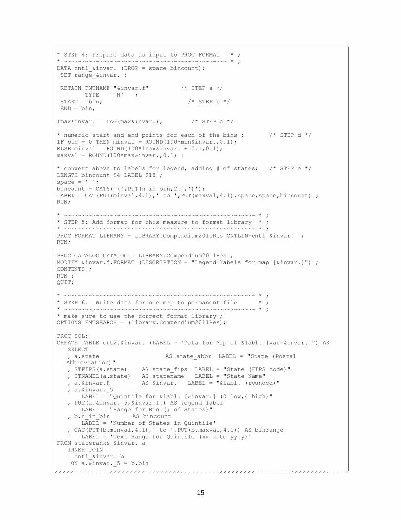
* STEP 4: Prepare data as input to PROC FORMAT * ;
* ~~~~~~~~~~~~~~~~~~~~~~~~~~~~~~~~~~~~~~~~~~~~~~ * ;
DATA cntl_&invar. (DROP = space bincount);
SET range_&invar. ;
RETAIN FMTNAME "&invar.f" /* STEP a */
TYPE 'N' ;
START = bin; /* STEP b */
END = bin;
lmax&invar. = LAG(max&invar.); /* STEP c */
* numeric start and end points for each of the bins ; /* STEP d */
IF bin = 0 THEN minval = ROUND(100*min&invar.,0.1);
ELSE minval = ROUND(100*lmax&invar. + 0.1,0.1);
maxval = ROUND(100*max&invar.,0.1) ;
* convert above to labels for legend, adding # of states; /* STEP e */
LENGTH bincount $4 LABEL $18 ;
space = ' ';
bincount = CATS('(',PUT(n_in_bin,2.),')');
LABEL = CAT(PUT(minval,4.1),' to ',PUT(maxval,4.1),space,space,bincount) ;
RUN;
* ~~~~~~~~~~~~~~~~~~~~~~~~~~~~~~~~~~~~~~~~~~~~~~~~~~~~~~ * ;
* STEP 5: Add format for this measure to format library * ;
* ~~~~~~~~~~~~~~~~~~~~~~~~~~~~~~~~~~~~~~~~~~~~~~~~~~~~~~ * ;
PROC FORMAT LIBRARY = LIBRARY.Compendium2011Res CNTLIN=cntl_&invar. ;
RUN;
PROC CATALOG CATALOG = LIBRARY.Compendium2011Res ;
MODIFY &invar.f.FORMAT (DESCRIPTION = "Legend labels for map [&invar.]") ;
CONTENTS ;
RUN ;
QUIT;
* ~~~~~~~~~~~~~~~~~~~~~~~~~~~~~~~~~~~~~~~~~~~~~~~~~~~~~~ * ;
* STEP 6. Write data for one map to permanent file * ;
* ~~~~~~~~~~~~~~~~~~~~~~~~~~~~~~~~~~~~~~~~~~~~~~~~~~~~~~ * ;
* make sure to use the correct format library ;
OPTIONS FMTSEARCH = (library.Compendium2011Res);
PROC SQL;
CREATE TABLE out2.&invar. (LABEL = "Data for Map of &labl. [var=&invar.]") AS
SELECT
, a.state AS state_abbr LABEL = "State (Postal
Abbreviation)"
, STFIPS(a.state) AS state_fips LABEL = "State (FIPS code)"
, STNAMEL(a.state) AS statename LABEL = "State Name"
, a.&invar.R AS &invar. LABEL = "&labl. (rounded)"
, a.&invar._5
LABEL = "Quintile for &labl. [&invar.] (0=low,4=high)"
, PUT(a.&invar._5,&invar.f.) AS legend_label
LABEL = "Range for Bin (# of States)"
, b.n_in_bin AS bincount
LABEL = 'Number of States in Quintile'
, CAT(PUT(b.minval,4.1),' to ',PUT(b.maxval,4.1)) AS binrange
LABEL = 'Text Range for Quintile (xx.x to yy.y)'
FROM stateranks_&invar. a
INNER JOIN
cntl_&invar. b
ON a.&invar._5 = b.bin

16
ORDER BY state ;
QUIT;
* Testing ;
PROC PRINT DATA = out.&invar. (obs=10);
ID state_abbr ;
run;
PROC CONTENTS DATA = out.&invar. ;
RUN;
%MEND mklegend ;
%MACRO mapmac(figtit,invar,year);
* ~~~~~~~~~~~~~~~~~~~~~~~~~~~~~~~~~~~~~~~~~~~~~~~~~~~~~~ * ;
* Step 7b: Build macro vars for the labels *
* ~~~~~~~~~~~~~~~~~~~~~~~~~~~~~~~~~~~~~~~~~~~~~~~~~~~~~~ * ;
PROC FREQ DATA=out.&invar.;
TABLES &invar._5*legend_label / NOPRINT OUT=legend;
RUN;
DATA _NULL_;
LENGTH tvar $ 2;
SET legend;
tvar=CATS("T",PUT(&invar._5 + 1, 1.));
CALL SYMPUT(tvar,legend_label) ;
RUN;
* ~~~~~~~~~~~~~~~~~~~~~~~~~~~~~~~~~~~~~~~~~~~~~~~~~~~~~~ * ;
* STEP Step 7c – produce the map and legend * ;
* ~~~~~~~~~~~~~~~~~~~~~~~~~~~~~~~~~~~~~~~~~~~~~~~~~~~~~~ * ;
OPTIONS ORIENTATION=landscape NODATE NONUMBER;
GOPTIONS DEVICE=png NOBORDER;
ODS LISTING CLOSE;
ODS HTML PATH=odsout BODY="&invar._&year..htm" OPTIONS(pagebreak='no');
GOPTIONS cback=white;
GOPTIONS GUNIT=pct FTITLE="albany amt/bold" FTEXT="albany amt/bold";
GOPTIONS HTITLE=18pt HTEXT=11pt CTITLE=black CTEXT=gray55;
LEGEND1 LABEL=none ACROSS=5 CSHADOW=dodgerblue CFRAME=gold CBLOCK=dodgerblue
POSITION=(bottom center outside) SHAPE=bar(.15in,.15in) MODE=reserve
OFFSET=(0,0) VALUE=("&t1" "&t2" "&t3" "&t4" "&t5");
PATTERN1 VALUE=msolid COLOR=white;
PATTERN2 VALUE=msolid COLOR=lightblue ;
PATTERN3 VALUE=msolid COLOR=CornflowerBlue ;
PATTERN4 VALUE=msolid COLOR=blue ;
PATTERN5 VALUE=msolid COLOR=navy;
TITLE1 a=-90 h=5pct " ";
TITLE2 a=90 h=1pct " ";
DATA my_data;
SET out.&invar. (RENAME=(state_fips=state statename=state_name));
LENGTH my_html $100;
my_html='TITLE='||QUOTE(TRIM(LEFT(state_name))||': '||
TRIM(LEFT(PUT(&invar.*100,5.1))) );
RUN;

17
PROC GMAP DATA=my_DATA MAP=mymap ALL ANNO=extra_label;
ID state_name;
CHORO &invar._5 / DISCRETE COUTLINE=gold WOUTLINE=1
CDEFAULT=yellow
LEGEND=legend1
HTML=my_html
DES='' NAME="&invar._&year";
RUN;
QUIT;
ODS _all_ CLOSE;
ODS LISTING;
%MEND mapmac;
%MACRO gen508(fignum,figvar,figtit,figyear,lctit,outfi,source);
* ~~~~~~~~~~~~~~~~~~~~~----~~~~~~~~~~~~~~~~~~~~~~~~~~~~~~~~~ * ;
* Step 8a – Generate bin-level data set from state-level one * ;
* ~~~~~~~~~~~~~~~~~~~~~----~~~~~~~~~~~~~~~~~~~~~~~~~~~~~~~~~ * ;
PROC SORT DATA = out.&figvar. (keep = &figvar._5 legend_label bincount binrange)
OUT = step8a NODUPKEY ;
BY legend_label ;
RUN;
* ~~~~~~~~~~~~~~~~~~~~~----~~~~~~~~~~~~~~~~~~~~~~~~~~~~~~~~~~~~~~~ * ;
* Step 8b - transpose state level measure data set to get * ;
* lists of states by legend labels for the measure level bins * ;
* ~~~~~~~~~~~~~~~~~~~~~----~~~~~~~~~~~~~~~~~~~~~~~~~~~~~~~~~~~~~~~ * ;
PROC SORT DATA=out.&figvar. (KEEP = statename legend_label) OUT=&figvar._st ;
BY legend_label statename;
RUN;
PROC TRANSPOSE DATA=&figvar._st (KEEP=statename legend_label)
OUT=step8b (DROP = _:) PREFIX=st_;
VAR statename;
BY legend_label;
RUN ;
* put the largest binsize into a macro variable ;
PROC SQL ;
SELECT LEFT(PUT(MAX(bincount),2.)) INTO: Nmaxbin
FROM step8a;
QUIT;
%PUT &Nmaxbin;
* ~~~~~~~~~~~~~~~~~~~~~----~~~~~~~~~~~~~~~~~~~~~~~~~~~~~~~~ * ;
* Step 8c – String the states out into a sentence * ;
* ~~~~~~~~~~~~~~~~~~~~~----~~~~~~~~~~~~~~~~~~~~~~~~~~~~~~~~ * ;
DATA step8c;
LENGTH numword $ 10 stlist $ 2000 ;
MERGE step8a step8b;
BY legend_label;
legend_label=COMPBL(legend_label);
***Get number words for each legend label group;
Numword =PROPCASE(PUT(bincount,WORDS10.)) ;
stlist = st_1;

18
ARRAY stnames {&Nmaxbin.} st_1 - st_&Nmaxbin. ;
IF bincount = 2 THEN stlist = CATX(' ',stlist,'and',st_2) ;
ELSE IF bincount > 2 THEN DO;
DO i = 2 TO (bincount - 1) ;
stlist = CATX(', ',stlist,stnames{i}) ;
END;
stlist = CATX(' ',stlist,'and',stnames{bincount}) ;
END;
* add a period at end of list ;
stlist = catt(stlist,'.');
DROP i;
RUN;
* ~~~~~~~~~~~~~~~~~~~~~----~~~~~~~~~~~~~~~~~~~~~~~~~~~~~~~~~~ * ;
* Step 8d: Prepare the final paragraph for PROC REPORT * ;
* ~~~~~~~~~~~~~~~~~~~~~----~~~~~~~~~~~~~~~~~~~~~~~~~~~~~~~~~~ * ;
DATA sent1 (RENAME=(stlist=sent1 numword=num1 binrange=range1 ))
sent2 (RENAME=(stlist=sent2 numword=num2 binrange=range2))
sent3 (RENAME=(stlist=sent3 numword=num3 binrange=range3))
sent4 (RENAME=(stlist=sent4 numword=num4 binrange=range4))
sent5 (RENAME=(stlist=sent5 numword=num5 binrange=range5));
SET Step8c (KEEP=&figvar._5 stlist numword binrange);
IF &figvar._5=0 THEN OUTPUT sent1;
ELSE IF &figvar._5=1 THEN OUTPUT sent2;
ELSE IF &figvar._5=2 THEN OUTPUT sent3;
ELSE IF &figvar._5=3 THEN OUTPUT sent4;
ELSE IF &figvar._5=4 THEN OUTPUT sent5;
RUN;
DATA Step8d;
LENGTH blurb blurb1 - blurb5 $ 20000 figtit lctit source $ 132;
MERGE sent1-sent5;
lctit="&lctit";
fignum="&fignum";
figtit="&figtit";
source=CATS('^n^n',"&source.");
constant_text1='Figure';
constant_text2=
'. This is a five color map of the United States that displays the';
constant_text3='states have';
constant_text4='for each state.';
constant_text5=
'Guam, Puerto Rico and the Virgin Islands are not included in this figure.';
blurb1=CATX(' ',num1,constant_text3,range1,lctit,sent1);
blurb2=CATX(' ',num2,constant_text3,range2,lctit,sent2);
blurb3=CATX(' ',num3,constant_text3,range3,lctit,sent3);
blurb4=CATX(' ',num4,constant_text3,range4,lctit,sent4);
blurb5=CATX(' ',num5,constant_text3,range5,lctit,sent5);
blurb=
CATX(' ',constant_text1,fignum,constant_text2,figtit,constant_text4,
blurb1,blurb2,blurb3,blurb4,blurb5,constant_text5,source);
blurb=COMPBL(blurb);
RUN;
* ~~~~~~~~~~~~~~~~~~~~~----~~~~~~~~~~~~~~~~~~~~~~~~~~~~ * ;
* Step 8e - Report on the paragraph just created *;
* ~~~~~~~~~~~~~~~~~~~~~----~~~~~~~~~~~~~~~~~~~~~~~~~~~~ * ;
ODS LISTING CLOSE;
ODS ESCAPECHAR='^';
ODS RTF FILE="&figvar._&figyear..rtf" PATH=odsout STYLE=styles.noborder;

19
TITLE2 "Figure &fignum. - &figyear. - Section 508 compliance text";
PROC REPORT NOWD DATA=step8d
STYLE(REPORT)=[CELLPADDING=3pt VJUST=b]
STYLE(HEADER)=[JUST=center FONT_FACE=Helvetica FONT_WEIGHT=bold
FONT_SIZE=10pt]
STYLE(LINES)=[JUST=left FONT_FACE=Helvetica] ;
COLUMNS blurb ;
DEFINE blurb / STYLE(COLUMN)={JUST=l FONT_FACE=Helvetica
FONT_SIZE=10pt CELLWIDTH=1000 }
style(HEADER)={JUST=l FONT_FACE=Helvetica
FONT_SIZE=10pt };
RUN;
ODS RTF CLOSE;
ODS LISTING ;
%MEND gen508;
***A few example calls to the macros;
%mklegend(invar=Age_ge95,labl=% of Residents Age 95 and older)
%mklegend(invar=ADLimp0,labl=% of Residents with 0 ADL impairments)
%mklegend(invar=Falls_any,labl=% of Residents with Any Recent Falls)
%mklegend(invar=Antipsych,labl=% of Residents Taking Antipsychotic Medication)
%mapmac(Figure 3.16,antipsych,2011);
%gen508(3.16,
antipsych,
percentage of nursing home residents taking antipsychotic medication,
2011,
percent of nursing home residents taking antipsychotic medication including,
fig316_508,
The source of data for this figure is the Minimum Data Set.);
CONCLUSION
What started as a fairly basic analytic and data manipulation problem of assigning states to categories of a measure for purposes of mapping became an interesting formatting task because of the need to label the categories in a specific way and the need to make the process reproducible – from measure to measure and year to year. Further, the need to do precisely the same set of manipulations for dozens of measures made the job an obvious candidate for macros. In my view, the real “trick” here is using PROC SUMMARY and PROC SQL to reveal (and document) the thresholds between the quintile categories from the data produced by PROC RANK – which assigns the categories for the current data but doesn’t “tell” us what those breakpoints are. I hope that there are a few other simple techniques in this process that you’ll find useful as well, such as the automated production of attractive, data-driven maps and text to help enable Section 508 compliance.
There are some obvious possible extensions of the code. With relatively little revision, the macro could be (and has been) extended to process data for multiple years, different numbers of categories for different measures, different levels of precision. We’ve also extended it to accommodate new data – where we don’t want the basic categories to change, but we may need to extend the overall range because of secular trends in the data. Briefly, we can pull the previous year’s information out of the formats (using the CNTLOUT option), check if the ranges need to be extended, generate new formats to assign the new data into the (mostly) unchanged bins, and, of course, re-generate the counts of states going into each bin.

20
As with many projects, this task has evolved over time. Currently, we have combined the small measure data sets into a single long data set (with a row for each measure for each state), so that the same information and structure is available with a variable denoting which measure the data is for. We have also added information on figure titles, which we inserted with macro variables above. We hope to incorporate pulling in information on figure numbers and titles from a metadata spreadsheet maintained for a given year’s processing in the future.
REFERENCES
Centers for Medicare and Medicaid Services, “Nursing Home Data Compendium 2013 Edition”, Available at https://www.cms.gov/Medicare/Provider-Enrollment-and-
Certification/CertificationandComplianc/downloads/nursinghomedatacompendium_508.pdf
Hadden, Louise. 2014. “Extreme SAS® Reporting II: Data Compendium and 5 Star Ratings Revisited” Proceedings of SAS Global Forum 2014. Available at http://support.sas.com/resources/papers/proceedings14/1342-2014.pdf
Williams, Christianna. 2014. “PROC RANK, PROC SUMMARY, and PROC FORMAT Team Up and a Legend is Born!” Proceedings of SESUG 2014. Available at http://analytics.ncsu.edu/sesug/2014/AD-07.pdf
Allison, Robert. 2012. SAS/GRAPH: Beyond the Basics. Cary, NC: SAS Institute Inc.
Zdeb, Mike. 2002. Maps Made Easy Using SAS. Cary, NC: SAS Institute Inc.
RECOMMENDED READING
Robert Allison’s examples: http://robslink.com/SAS/Home.htm
Specific example used: http://www.robslink.com/SAS/democd54/natural_disasters_info.htm).
e-book: http://robslink.com/SAS/book1/
ACKNOWLEDGMENTS
The authors gratefully acknowledge the contributions of several CMS colleagues, including Edward Mortimore, Jon Friedlander, Dan Andersen and Ian Kramer. In addition, we appreciate the creative and helpful examples, and technical assistance provided by Robert Allison of SAS,
CONTACT INFORMATION
Your comments and questions are valued and encouraged. Contact the authors at:
Name: Christianna Williams E-mail: [email protected]
Name: Louise Hadden E-mail: [email protected]
SAS and all other SAS Institute Inc. product or service names are registered trademarks or trademarks of SAS Institute Inc. in the USA and other countries. ® indicates USA registration.
Other brand and product names are trademarks of their respective companies.