Embed Size (px)
Citation preview
Panel Data Estimation Methods on Supply
and Demand Elasticities: The Case of
Cotton in Greece
Christina Kotakou
This article examines the effects of the application of panel data estimation methods ona system of equations with unbalanced panel data. We apply pooled, random-effects, andfixed-effects estimation in three data sets: small, medium, and large farms to examine therelationship between farm size and the elasticity of cotton supply with respect to cotton price.Our results indicate that the adoption of various estimation methods entails different esti-mated parameters both in terms of their absolute value and in terms of their statistical sig-nificance. Additionally, the elasticity of cotton supply with respect to price varies accordingto farm size.
Key Words: farm size, panel data, supply elasticity, systems of equations
JEL Classifications: C33, D21, Q18
In recent years, many empirical studies that
evaluate the effects of agricultural policies in
Europe and United States have relied on data
sets that are balanced or unbalanced panels.
The use of farm-level data implies that we have
to consider the application of proper panel data
estimation methods so as to obtain estimates of
parameters. The adoption of the appropriate
estimation method is crucial because the esti-
mated parameters are used for policy evalua-
tion. Consequently, the increased reliability of
the estimated parameters ensures that the pol-
icy evaluation will be more accurate.
Although there are a significant number of
empirical papers that rely on the estimation of
a system of equations with balanced or un-
balanced panel data to evaluate agricultural
policies, they do not use panel data estimation
methods. Serra et al. (2005a, 2006) examined
the effects of agricultural policies in the United
States. They have estimated a system of equa-
tions using a balanced panel with farm-level data
collected in Kansas. As for the unbalanced panel
data sets, the most frequently used in agricultural
economics in the European Union is the Farm
Accountancy Data Network (FADN), which
consists of farm-level data collected every year
(Bakucs and Ferto, 2009; Csajbok, Lansink, and
Huirne, 2005; Karagiannis and Sarris, 2005;
Melfou, Theocharopoulos, and Papanagiotou,
2009; Reidsma et al., 2009; Rezitis, Tsiboukas,
and Tsoukalas, 2002). Many studies that eval-
uate the effects of Common Agricultural Policy
estimate a system of equations and make use of
the FADN data set. However, they do not take
into account the panel structure of the data
(Moro and Sckokai, 1999; Sckokai and Moro,
2006; Serra et al., 2005b).
In this study we focus on the estimation
of a Seemingly Unrelated Regression System
Christina Kotakou is a PhD candidate, Department ofEconomics, University of Macedonia, Thessaloniki,Greece.
I thank Jeffrey Gillespie and two anonymous re-viewers for their useful comments and suggestions.
Journal of Agricultural and Applied Economics, 43,1(February 2011):111–129
� 2011 Southern Agricultural Economics Association
(SUR) with unbalanced panel data applying
three estimation techniques: pooled, random-
effects (RE), and fixed-effects (FE) estimation.
We apply these methods to underline the dif-
ferent results obtained by adopting them. The
effects of panel data estimation methods on
estimated parameters have also been examined
by Platoni, Sckokai, and Moro (2008). However,
although they apply FE and RE estimation in
a single equation, in a system of equations only,
the RE method is applied. In this study, we apply
all the different estimation techniques in a sys-
tem of equations, i.e., in the same model. Thus,
the difference in the estimated parameters is
exclusively attributed to the estimation method.
In terms of economic analysis, the objective
of this study is to examine the relationship be-
tween farm size and the elasticity of cotton
supply with respect to its own price. The elas-
ticities we estimate are short-run elasticities,
which, generally, are smaller than the long-run
supply elasticities as a result of the existence of
fixed costs. Although producers in the short run
can increase production by increasing variable
inputs, in the long run, producers can adjust all
input quantities. Small farmers use more vari-
able inputs than medium and large farmers
(European Commission, 2007, pp. A6–A13).
This way, small farmers gain in terms of flex-
ibility and therefore can better accommodate to
output variation in the presence of price fluctu-
ations (Mills and Schumann, 1985). Therefore,
we expect the elasticity of the cotton supply to be
decreasing with respect to farm size. This result
was found by Adesoji (1991), who examined the
relation of farm size and supply elasticity for
U.S. dairy farms. He found that they move in the
opposite direction in the short run but the reverse
holds during the long-run period.
The European Union Cotton Market
The cotton sector is of limited importance to
the European Union (EU) as a whole because
cotton contributes only 0.5% to the final agri-
cultural output. However, cotton production has
strong regional importance to Greece and Spain,
which are the main EU cotton producers. Greece
is the major cotton-producing Member State of
the EU given that 76% of the EU’s total cotton
output is grown in Greece. The share of cotton to
total agricultural output in Greece is 9.1% and in
Spain 1.3% (European Commission, 2007).
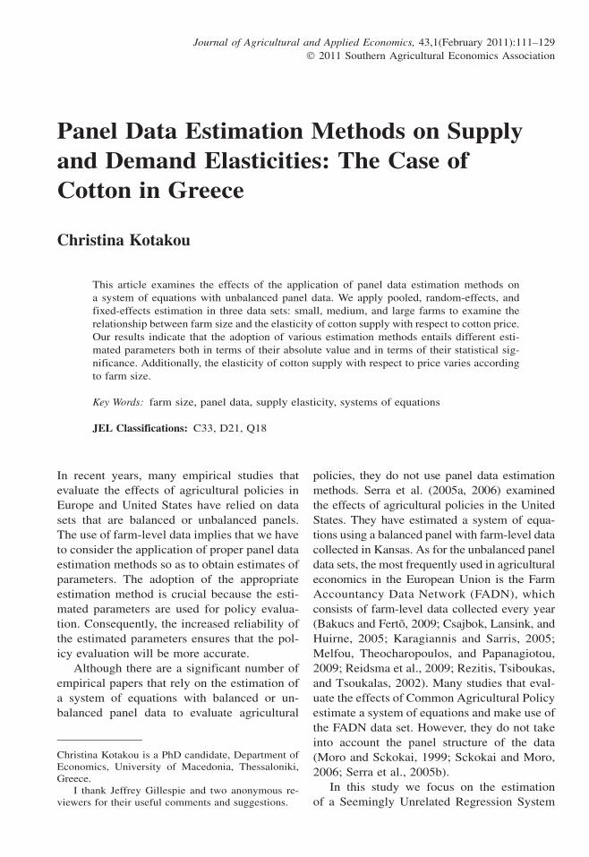
In terms of economic size classes, i.e., the
classification that is used in the present study,
the distribution of small-, medium-, and large-
sized cotton farms in Greece and Spain is pre-
sented in Table 1.
In light of these results, it is quite clear that
the number of cotton farmers in Greece is much
Table 1. Distribution of Cotton Farms per Size Category in Greece and Spain
Number of Cotton Farms per Size Category
2000 2003 2005 2007
Greece Spain Greece Spain Greece Spain Greece Spain
Small farms 16.600 840 15.810 780 15.550 490 13.200 80
Medium farms 14.930 1.490 10.670 460 11.980 1.200 12.220 200
Large farms 10.520 1.930 5.720 1.390 5.980 1.290 7.510 1.420
Total 42.050 4.260 32.200 2.630 33.510 2.980 32.930 1.700
Share of Cotton Farms per Size Category to Total Number of Cotton Farms
2000 2003 2005 2007
Greece Spain Greece Spain Greece Spain Greece Spain
Small farms 39.48% 19.72% 49.10% 29.66% 46.40% 16.44% 40.09% 4.71%
Medium farms 35.51% 34.98% 33.14% 17.49% 35.75% 40.27% 37.11% 11.76%
Large farms 25.02% 45.31% 17.76% 52.85% 17.85% 43.29% 22.81% 83.53%
Source: Farm Accountancy Data Network.
Journal of Agricultural and Applied Economics, February 2011112

larger than in Spain. For example, the total
number of cotton farms in Greece in 2000 is
42.050, in which 16.600 are small and 14.930
and 10.250 are medium and large, respectively.
The total number of cotton farms in Spain in
2000 is 4.260, which corresponds to 840 small,
1.490 medium, and 1.930 large farms. In both
countries, the number of cotton farms decreases
from 2000 to 2003 but in Greece remains rel-
atively stable after 2003. On the other hand, the
number of cotton farms in Spain reduces
greatly in 2007. This result can be attributed to
the change in the cotton policy regime that took
place in the EU from 2006. In Spain, during the
cultivation year 2006–2007, there was a de-
crease in the area under cotton by 45%. On the
contrary, in Greece, the cotton area increased
by 4% (European Commission, 2007).
Taking into consideration the share of farms
per size, it is clear that there is small change
from year to year in Greece. However, the sit-
uation in Spain is completely different. The
share of small and medium farms to total cotton
producers gradually decreases and the corre-
sponding share of large farms is almost doubled
from 2000 to 2007. According to the FADN
data, the total cost of production is higher in
Spain, 3.037 V/ha, than in Greece, 2565 V/ha.
Additionally, the total profit is larger in Spain,
745.5 V/ha, than in Greece, 596.8 V/ha (European
Commission, 2007).
Theoretical Framework
In this section, we present the theoretical
framework that we used in this study. To com-
pute the supply and the derived demand elas-
ticities, we use duality theory and particularly
a flexible functional form of profit function.
Flexible functional forms of profit functions
have been widely used in agricultural economics
research (Abrar, Morrissey, and Rayner, 2004;
Arnade and Kelch, 2007; Pope et al., 2007;
Shumway, 1983; Sidhu and Baanante, 1981;
Vilezca-Becerra and Shumway, 1994; Weaver,
1983). We choose the normalized quadratic
profit function, which is one of the flexible
functional forms that exist.
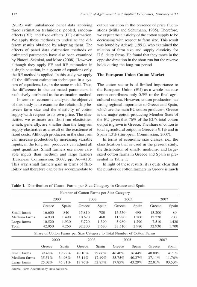
The normalized quadratic profit function
has the following form:
(1)
P =Pm 5 ao 1Xm�1
i51
ai Pi =Pmð Þ1Xn
i5m11
biZi
11
2
Xm�1
i51
Xm�1
j51
aij Pi =Pmð Þ Pj =Pm
� �
11
2
Xn
i5m11
Xn
j5m11
bijZiZj
1Xm�1
i51
Xn
j5m11
g ij Pi =Pmð ÞZj 1 d1t
11
2d2t2 1
Xm�1
i51
ei Pi =Pmð Þt
1Xn
i5m11
ziZit
where P is short-run profit (revenue minus
variable costs) divided by the price of netput m
(input or output); P1. . . .Pm21 are the prices of
the rest netputs (netputs are measured in neg-
ative units if they are inputs and in positive
units in case that they refer to outputs) divided
by the price of netput m; Zm11,. . .,Zn are the
quantities of quasifixed factors of production; t
is a time trend; and a, b, g , d, e, z are param-
eters to be estimated.
Applying Hotelling’s lemma to equation (1)
we obtain the supply of output yi, and the de-
rived demands for variable inputs of production
xi:
(2)
›P›ðPi =PmÞ
5 yi 5 ai 1Xm�1
j51
aijðPj =PmÞ
1Xn
j5m11
g ijZj 1 eit
(3)
›P›ðPi =PmÞ
5�xi 5 ðai 1Xm�1
j51
aijðPj =PmÞ
1Xn
j5m11
g ijZj 1 eitÞ
for i51.....m� 1
To be consistent with competitive theory, the
profit function must satisfy the following prop-
erties: linear homogeneity in prices, symmetry,
i.e., aij 5 aji, monotonicity in prices and fixed
inputs, convexity in prices, and concavity in
quantities of fixed inputs. We impose linear ho-
mogeneity by dividing the profit function with
Kotakou: Supply and Demand Elasticities of Cotton 113
the price of m netput (in our case input)1 and
symmetry before estimation. Convexity and
monotonicity were checked after estimation.
Econometric Techniques
In this section, we present the econometric tech-
niques that we applied to obtain estimators of the
coefficients. As we noted in the introductory
comments, we estimate a system of equations
using three different econometric techniques.
In the first case, we estimate the system without
taking into consideration the panel specifica-
tion of our data, i.e., pooled estimation. In the
second case, we estimate the system using the
one-way error components method for unbal-
anced panel data proposed by Biørn (2004) so
as to obtain RE estimators. Finally, we use the
least-squares dummy-variable approach to ob-
tain the FE estimators.2
A. Pooled Data Estimation
It is well known that the appropriate way to
estimate a system of M equations is the SUR
proposed by Zellner (1962). In this case, the
best linear unbiased estimator is the General-
ized Least Squares (GLS). Up to now, this
method has been used by various researchers in
agricultural economics (Carlberg, 2002; Fousekis
and Revell, 2000; Lee, Kennedy, and Fletcher,
2006).
B. Panel Data Estimation
The panel data estimation relies on the hypoth-
esis that in the estimation procedure, we take
into account the ‘‘heterogeneity’’ of each cross-
sectional unit. Because it is well known by pre-
vious studies (Baltagi, 1985; Cai et al., 2008;
El-Osta and Mishra, 2005; Kaltsas, Bosch, and
McGuirk, 2008; Poudel, Paudel, and Bhattarai,
2009), the most frequently used models in panel
data are the one-way RE and FE models. These
models rely on the hypothesis that differences
among cross-sectional units can be captured by
means of an intercept term, which is specific for
each cross-sectional unit. This specific intercept
term is considered as a random disturbance in
the RE model and as a fixed parameter in the FE
model.
B1. One-way Random-effects Model. Avery
(1977) was the first to suggest an appropriate
method of estimating a SUR system with er-
ror components when the data set is a bal-
anced panel. However, in most cases, we have
to deal with unbalanced panels so we have to
apply the method proposed by Biørn (2004).
The main difficulty in applying both methods
is that no econometric software supports the
estimation of a SUR system with error com-
ponents either for a balanced or for un-
balanced data set. In the following analysis,
we provide the approach suggested by Biørn
(2004), which we use in the present study.
Consider a system that consists of M re-
gression equations indexed by m 5 1,...., M.
The data set is an unbalanced panel with N
farms indexed by i 5 1,....,N, where each farm
is observed in at least two and at most S periods.
Let Ds denote the number of farms observed in
s periods with s 5 2,....S, and n corresponds to
the total number of observations. Then the total
number of farms observed up to S periods and
the total number of observations are given by
D 5PS
s52 Ds and n 5PS
s52 Dss, respectively.
The farms are ordered in S groups so as the D2
farms observed twice come first, the D3 farms
observed three times come second, etc. If the
cumulative number of farms observed up to
1 The derived demand equation for the numeraireinput is given by the expression:
xm 5 P =Pm �Xm�1
i51
Pi›P
›ðPi =PmÞ5a0
1Xn
i5m11
biZi �1
2
Xm�1
i51
Xm�1
j51
aijðPi =PmÞðPj=PmÞ
11
2
Xn
i5m11
Xn
j5m11
bijZiZj 1 d1t 11
2d2t2
1Xn
i5m11
ziZit
which is a quadratic function of normalized prices,quasi-fixed factors of production and time trend.
2 To apply the FE estimation method, we had toeliminate all the farms that appeared only once in thesamples.
Journal of Agricultural and Applied Economics, February 2011114

s times is Ks, then the index sets of the farms
observed s times can be written as:
(4)
I2 5 1,..........,K2
I3 5 K2 1 1,.....,K3
..
.
IS 5 KS�1 1 1,.....,KS
where I2,. . .,IS can be considered as balanced
subpanels with 2, . . . . ,S observations of each
farm, respectively.
The system of M equations for individual i,
observation t3 is written as:
(5)ymit 5 Xmitbm 1 dmi 1 lmit 5 Xmitbm 1 umit
m 5 1,....M,i 2 Is,t51,....S
The dimensions of the matrices consisting of
ymit, Xmit, and bm are Mn � 1, Mnx k and k � 1,
respectively.
The usual assumptions made by ECM are:
(6)
Eðdmi,dji0 Þ 5 s2dmj i 5 i0
5 0 i 6¼ i0
Eðlmit,lji0t0 Þ 5 s2lmj i 5 i0,t 5 t0
5 0 i 6¼ i0,t 6¼ t0
where i is the farm index and t is the sequence
index, which counts the times that each farm is
observed.
The variance–covariance matrix of the re-
siduals in this case is equal to:
(7) VuðsÞ5Cs � Sl 1 Fs � ðSl 1 sSdÞ
where Fs 5 (1/s)Hs and Cs 5 Is – (1/s)Hs, Is is the
identity matrix of dimension s, and Hs 5 hshs9 is
the (sxs) matrix with all elements equal to one.
To compute the matrices Sl and Sd, we
have to calculate the (M�M) matrices of overall
within farms and between farms (co)variation in
the residuals u of the different equations, which
can be expressed as:
(8) Wuu 5XS
s52
Xi2Is
Xs
t51
ðuit � �uiÞðuit � �uiÞ0
(9) Buu 5XS
s52
Xi2Is
sð�ui � �uÞð�ui � �uÞ0
where �ui 5 ð1=sÞPst 51
uit and �u5 ð1=nÞPSs52
Pi2Is
sui.
Biørn (2004) proved that the matrices Sland Sd are given by the following expressions:
(10) S l5Wuu
n� N
(11) Sd5Buu � ððN � 1Þ=ðn� NÞÞWuu
n�PS
s52 Dss2� �
=n
Using equations (8) and (9) to obtain estimates
of the variance–covariance matrices Sl and
Sd, these estimates are then substituted into
equation (7). After the calculation of the var-
iance–covariance matrix of the residuals, the
coefficient’s GLS estimators and their vari-
ance–covariance matrix can be computed by
the following formulas:
(12)
bGLS 5XS
s52
Xi2Is
X0
i sð ÞW�1u sð ÞXi sð Þ
!�1
�XS
s52
Xi2Is
X0
i sð ÞW�1u sð Þyi sð Þ
!
(13) V bGLS
� �5
XS
s52
Xi2Is
X0
i sð ÞW�1u sð ÞXi sð Þ
!�1
Once again, because there does not exist any
standard econometric software that provides au-
tomatic commands to estimate one-way SUR
systems, we applied the following stepwise pro-
cedure for estimating the W�1u sð Þ, the coefficient’s
GLS estimators, and their variance–covariance
matrix:
Step 1: We run an OLS regression separately
on all M equations for all observations yit and
Xit. Using our estimation results, we form the
corresponding vectors of residuals uit 5 yit �XitbOLS for all i and t.
Step 2: We compute the matrices of overall
within and between farms (co)variation that is
Wuu,Buu by inserting the residuals uitin equa-
tions (8) and (9).
Step 3: We calculate matrices Sl,Sd by
inserting the matrices Wuu,Buu in expressions
(10) and (11).3 In this case, t is a sequence index, not a time
index.
Kotakou: Supply and Demand Elasticities of Cotton 115
Step 4: Using the results from the previous
step and equation (7), we calculate the variance–
covariance matrix Wu sð Þ.Step 5: We compute the matrix W�1
u sð Þ, which
is inserted in equations (12) and (13) so as to
calculate the GLS estimators as well as their
variance–covariance matrix.
B2. One-way fixed-effects Model. To obtain
the FE estimators we follow the procedure
that is described in the previous section but
we modified the variance–covariance matrix
of the residuals. It is well known that the GLS
estimator is a weighted average of the be-
tween and within group estimators (Hsiao,
1986, p. 36). In the case that we exclude the
between-group variation in the residuals from
the variance–covariance matrix, we obtain
the within-group or FE estimators. According
to this property of GLS estimator, we modified
the variance–covariance matrix described in
equation (7) as follows:
(14) WFE 5 Cs � Sl
The FE estimators and their variance–covariance
matrix are given by the following formulas:
(15)
bFE 5XS
s52
Xi2Is
X0
i sð ÞV�1FEXi sð Þ
!�1
�XS
s52
Xi2Is
X0
i sð ÞV�1FEyi sð Þ
!
(16) V bFE
� �5
XS
s52
Xi2Is
X0
i sð ÞV�1FEXi sð Þ
!�1
Statistical Tests
In our analysis we make the hypothesis that the
estimated coefficients vary according with farm
size as well as with the estimation method. As
a result, it is necessary to examine if our hy-
potheses are valid by conducting some statistical
tests. To examine the statistical significance of
the differences in the estimated coefficients
among the different types of farm size, we used
the dummy variable approach proposed by
Guajarati (1970). According to this approach,
suppose that we have a set of N 5 N1 1 N2 1 N3
observations of the same variables and there is
a source of difference between the observations
of subsamples N1, N2, and N3. Then we run
a regression by pooling the set of N observations
and we use dummy variables in the coefficients
that are affected by this source of difference.
Consider, for example, the case that the source
of difference affects the constant term and the
slope coefficient, then we run a regression as
follows:
(17)yit 5 a1 1 a2D1 1 a3D2 1 b1Xit 1 b2D1Xit
1 b3D2Xit 1 eit
where D1 5 1 if the observation lies in the N2
set of observations
D1 5 0, otherwise
D2 5 1, if the observation lies in the N3 set
of observations
D2 5 0, otherwise
To test the hypothesis of no parameter change,
we have to test the joint hypothesis that
H0 : a2 5 a3 5 b2 5 b3 5 0 against the alter-
native that at least one of the four hypotheses
is not true. This test can be easily conducted
by using the c2J where J is the number of co-
efficients to be tested.
Additionally, we have to test which is the
appropriate specification of our model, i.e., the
pooled, the RE, or the FE. In the beginning, we
test the pooled against the one-way FE model
because the question of whether to pool the
data or not naturally arises with panel data. In
this case, we have to test the hypothesis that
constant terms are homogeneous or not (Hsiao,
1986, p. 16). The null and the alternative hy-
potheses are:
H0 : a1 5 a2 5 ........... 5 aN
H1 : a1 6¼ a2 6¼ ........... 6¼ aN
Under the null hypothesis, the constant term is
the same for all individuals and the pooled es-
timators are efficient. The null hypothesis rep-
resents a set of linear restrictions on coefficients
so we can test the null by using the F-statistic
written in terms of restricted and unrestricted
model sum of squares. In our case, because we
have a system of regression equations, we have
to use the generalized F test statistic (Bun, 2004;
Zellner, 1962). The F-statistic has the form:
Journal of Agricultural and Applied Economics, February 2011116

(18) F 5ðRRSS� URSSÞ=J
URSS=ðMNT � KÞ ; FðJ,MNT�KÞ
where RRSS 5 residual sum of squares of the
pooled model
URSS 5 residual sum of squares of the FE
model
J 5 number of linear restrictions equal with
M(N-1)
M 5 number of equations
NT 5 number of observations
K 5 number of estimated coefficients
Finally, we examine if the appropriate panel
model specification is the RE or the FE. The
critical assumption in the RE model is that
E uit =Xitð Þ5 0, i.e., there is no correlation be-
tween the included variables and the RE. If
there is correlation between the included vari-
ables and the RE, that is E uit =Xitð Þ 6¼ 0, the
RE estimators become biased and inconsistent
(Baltagi, 2005). Hausman (1978) provides a
test in which we compare these estimators.
Under the null hypothesis H0: E uit =Xitð Þ5 0
both estimators are consistent and the RE esti-
mator is efficient, whereas under the alternative
H1: E uit =Xitð Þ 6¼ 0 the FE estimator is consis-
tent but the RE estimator is not.
The test statistic is given by the expression:
(19) h 5 g0Y�1g
where g 5 bFE � bRE with bFE,bRE being the
vectors of estimated coefficients without the
constant terms and Y 5 VðbFEÞ � VðbREÞ.Under the H0, the test statistic h is asymptoti-
cally distributed as c2k where k is the dimension
of vector b.
Data
The data we use are from the EU FADN, Na-
tional Statistical Service of Greece and Euro-
stat during the period 1991–2002. From the
entire sample of farms that are characterized as
cotton producers, we use the farms that produce
only cotton as well as the farms that the pro-
portion of cotton revenue to total revenue is
equal or larger than 95%, so they are considered
as pure cotton producers. According to standard
FADN methodology, there are ten categories of
farm size and our sample consists of farms that
belong to first nine categories.4 Details about the
way that farms are grouping into nine categories
are provided in Table 2 in the Appendix. How-
ever, as a result of limitations in the number of
observations in each category, we grouped the
farms into three size categories. First, the farms
that belong to the first three categories are
considered small-sized. Second, the farms that
belong to the next three categories are consid-
ered as medium-sized and finally the farms of
the three last categories as large-sized. After
this grouping, we obtain three samples of un-
balanced panel data. The sample of small-sized
firms consists of 28 farms, the sample of me-
dium-sized farms involves 206 farms, and fi-
nally the sample of large-sized includes 282
agricultural enterprises.5 The number of obser-
vations of each sample is 108, 752, and 986 for
small, medium, and large farms, respectively.
The descriptive statistics of the variables are
provided in Table 3.
Cotton farmers produce cotton using four
variable inputs: labor, fertilizer, energy, and
other intermediate inputs6 and two quasi fixed
inputs: land and capital. Cotton quantity and
revenue are available from FADN data so we
obtain cotton price by dividing revenue with
quantity. As for the variable inputs, the FADN
sample contains expenditures and quantity of
labor, but only expenditures for fertilizer, en-
ergy, and the other intermediate inputs. Prices
for energy and fertilizer are provided by
Eurostat and the price index for the other in-
termediate inputs is provided by the National
Statistical Service of Greece. To obtain quan-
tities of energy and fertilizer, we divide the
expenditures by the corresponding prices. The
expenditures of the other intermediate inputs
are divided by their price index so as to obtain
their quantity measure. The quantity of land is
available from FADN data and the value of
4 Our sample does not contain farms that belong tothe tenth category because there are no so large cottonproducers in Greece.
5 The initial number of farms in each sample was75 small, 349 medium, and 456 large. However, weeliminated the farms that appeared only once in eachsample to apply the FE estimation method.
6 This category includes all other intermediate in-puts of production like water, pesticides, etc.
Kotakou: Supply and Demand Elasticities of Cotton 117

capital is deflated by the capital price index to
obtain its quantity measure. Finally, we include
a time trend to take into account the effect of
technology change in the cotton production.
For each sample of farms we estimate a
system of four equations: cotton supply and
the derived demands of fertilizer, energy, and
the other intermediate inputs. Labor is our
numeraire input. STATA 10 (College Station,
TX) econometrics software is used for the
estimations.
Estimation Results
In this section we present the estimated supply
and derived demand functions, which are ob-
tained by applying all estimation techniques, the
results of which are obtained by the statistical
tests as well as the elasticities for small-, me-
dium-, and large-sized farms. Initially, we pooled
the data for all farms to test if the parameter es-
timates differ by size. Using the dummy variables
approach, under the hypothesis that farm size
affects both constant terms and slopes, we found
that the differences in parameters are statistically
significant. The c252 statistic is equal to 965.73 at
the 5% level of significance with the corre-
sponding critical value 69.83. Estimation results
for small-, medium-, and large-sized farms are
reported in Tables 4, 5, and 6, respectively.
The absolute value of the estimated co-
efficients is fairly different when either com-
paring the coefficients of pooled with the
corresponding RE and FE or the coefficients of
RE with the FE. For example, the coefficient of
cotton supply with respect to cotton price for
large-sized farms is equal to 0.145, 0.244, and
0.330 when we apply the pooled, RE, and FE
methods, respectively. The statistical signifi-
cance of the estimated parameters is improved
when we apply the panel data estimation
methods. The standard errors of the RE coef-
ficients are smaller than the standard errors of
the pooled coefficients in 59 of 78 cases. The
result is similar when we compare the standard
errors of the FE estimators with the corre-
sponding of pooled estimators because they are
smaller in 43 of 66 cases. The obtained results
make clear that when we take into account
the panel specification of our data, the statis-
tical significance of the estimated parameters is
increased.
Additionally, we checked if the properties
of the profit function are satisfied. According to
the obtained results, the profit function is in-
creasing in the price of output and decreasing in
input prices. We also checked the eigenvalues
and the determinants of the principal minors of
Hessian matrix and we found that the only case
that the convexity property is not satisfied as
Table 3. Descriptive Statistics of the Variables
Variable
Small Farms Medium Farms Large Farms
Mean
Standard
Deviation Mean
Standard
Deviation Mean
Standard
Deviation
Profits (V) 1920.1 1486.25 5,928.92 4007.19 19,812.46 11,709.32
Cotton production (kilos) 7063.89 2134.91 17,083.51 5810.44 45,321.81 20,874.37
Cotton price (V/kilo) 0.80 0.06 0.80 0.07 0.81 0.07
Labor (hours) 797.58 236.67 1,283.70 579.57 2,165.75 1,030.54
Labor price (V/hour) 1.99 0.56 1.91 0.46 1.83 0.47
Energy quantity 558.07 385.59 1,756.92 1205.87 5,061.44 4,385.02
Energy price (V) 0.46 0.15 0.46 0.15 0.46 0.15
Fertilizer quantity 1713.66 659.48 4,205.70 1811.71 10,591.38 5,831.47
Fertilizer price (V) 0.18 0.03 0.18 0.03 0.18 0.03
Other intermediate inputs (V) 1207.79 520.14 2,584.96 1140.34 12,990.48 6,299.23
Other intermediate inputs
price (index)
185.51 30.51 185.51 30.51 185.51 30.51
Capital (V) 5870.54 5126.81 13,496.46 9521.70 27,764.78 18,646.8
Land (ha) 2.5 0.72 5.68 1.61 15.28 6.37
Journal of Agricultural and Applied Economics, February 2011118

Tab
le4.
Est
imat
edP
aram
eter
sof
Supply
and
Dem
and,
Sm
all-
Siz
edF
arm
s
Co
tto
nS
up
ply
Fer
tili
zer
Dem
and
En
erg
yD
eman
dO
ther
Inte
rmed
iate
Inp
uts
Dem
and
Var
iab
les
Po
ole
dR
EF
EP
oo
led
RE
FE
Po
ole
dR
EF
EP
oo
led
RE
FE
Co
nst
ant
0.2
98
0.1
74
—0
.51
20
.57
4—
1.4
24
1.0
64
—1
.25
72
.65
5—
(0.1
37
)(0
.14
7)
(0.1
85
)(0
.11
4)
(0.3
79
)(0
.11
6)
(0.5
11
)(0
.14
7)
Pri
ceo
fco
tto
n0
.82
32
.10
50
.87
4
(0.2
62
)(0
.29
9)
(0.3
06
)
Pri
ceo
ffe
rtil
izer
–0
.18
4–
0.2
63
–0
.41
6–
1.6
96
–1
.86
9–
1.9
19
(0.0
80
)(0
.07
0)
(0.0
80
)(0
.13
4)
(0.0
68
)(0
.07
1)
Pri
ceo
fen
erg
y–
0.0
53
–0
.15
4–
0.1
68
0.2
08
0.2
66
0.2
43
–1
.59
7–
1.5
91
–1
.64
4
(0.0
40
)(0
.04
3)
(0.0
51
)(0
.06
1)
(0.0
35
)(0
.03
7)
(0.1
26
)(0
.04
2)
(0.0
46
)
Pri
ceo
fo
ther
inte
rmed
iate
inp
uts
–0
.64
3–
2.1
47
–0
.49
61
.17
00
.80
80
.92
40
.42
40
.12
60
.19
5–
2.7
73
–2
.54
1–
1.2
64
(0.3
19
)(0
.33
7)
(0.3
28
)(0
.20
9)
(0.0
76
)(0
.08
1)
(0.1
64
)(0
.04
0)
(0.0
42
)(0
.64
0)
(0.4
05
)(0
.40
4)
Qu
anti
tyo
fca
pit
al0
.19
60
.38
10
.13
5–
0.1
98
–0
.09
2–
0.1
32
0.1
01
0.3
44
0.3
25
1.6
53
1.2
85
1.1
67
(0.0
85
)(0
.08
8)
(0.1
07
)(0
.12
3)
(0.0
72
)(0
.07
6)
(0.2
15
)(0
.06
6)
(0.0
72
)(0
.34
2)
(0.0
89
)(0
.09
3)
Qu
anti
tyo
fla
nd
0.3
14
0.3
57
0.2
78
–0
.16
1–
0.0
40
0.0
77
0.0
06
–0
.01
30
.06
5–
0.6
99
–0
.56
5–
0.9
12
(0.0
65
)(0
.07
4)
(0.0
99
)(0
.10
1)
(0.0
61
)(0
.05
9)
(0.2
03
)(0
.06
2)
(0.0
61
)(0
.25
9)
(0.0
65
)(0
.06
0)
Tim
etr
end
0.3
07
0.5
75
0.3
22
–0
.22
7–
0.0
31
0.1
19
1.0
75
0.8
52
1.0
44
–1
.37
8–
0.4
61
–1
.02
0
(0.1
04
)(0
.11
5)
(0.1
25
)(0
.13
4)
(0.0
88
)(0
.09
1)
(0.2
82
)(0
.09
2)
(0.0
96
)(0
.37
0)
(0.1
18
)(0
.10
5)
So
urc
e:O
wn
com
pu
tati
on
s.
No
te:
Nu
mb
ers
inp
aren
thes
esar
est
and
ard
erro
rs,
sig
nif
ican
tat
the
0.0
5le
vel
.
Kotakou: Supply and Demand Elasticities of Cotton 119

Tab
le5.
Est
imat
edP
aram
eter
sof
Supply
and
Dem
and,
Med
ium
-siz
edF
arm
s
Co
tto
nS
up
ply
Fer
tili
zer
Dem
and
En
erg
yD
eman
dO
ther
Inte
rmed
iate
Inp
uts
Dem
and
Var
iab
les
Po
ole
dR
EF
EP
oo
led
RE
FE
Po
ole
dR
EF
EP
oo
led
RE
FE
Co
nst
ant
0.2
20
0.2
07
—0
.14
20
.19
2—
0.5
49
0.4
90
—0
.18
10
.23
3—
(0.0
43
)(0
.05
0)
(0.0
68
)(0
.04
9)
(0.0
68
)(0
.04
8)
0.0
98
)(0
.05
0)
Pri
ceo
fco
tto
n0
.27
50
.24
20
.25
8
(0.0
67
)(0
.06
7)
(0.0
76
)
Pri
ceo
ffe
rtil
izer
–0
.21
2–
0.4
08
–0
.44
0–
1.0
98
–1
.24
8–
1.2
75
(0.0
27
)(0
.02
9)
(0.0
32
)(0
.04
5)
(0.0
32
)(0
.03
3)
Pri
ceo
fen
erg
y–
0.0
07
–0
.14
2–
0.1
94
0.2
70
0.2
40
0.2
16
–1
.48
5–
1.6
63
–1
.66
8
(0.0
22
)(0
.02
4)
(0.0
27
)(0
.03
0)
(0.0
21
)(0
.02
1)
(0.0
41
)(0
.02
7)
(0.0
29
)
Pri
ceo
fo
ther
inte
rmed
iate
inp
uts
–0
.07
40
.16
80
.22
60
.44
60
.27
60
.29
00
.62
80
.52
20
.49
5–
1.2
98
–0
.66
5–
0.5
72
(0.0
78
)(0
.07
3)
(0.0
80
)(0
.05
1)
(0.0
32
)(0
.03
3)
(0.0
43
)(0
.02
4)
(0.0
26
)(0
.11
7)
(0.0
92
)(0
.10
0)
Qu
anti
tyo
fca
pit
al0
.08
40
.04
20
.04
2–
0.0
43
–0
.01
9–
0.0
29
–0
.02
5–
0.0
43
–0
.06
60
.42
30
.34
00
.34
9
(0.0
15
)(0
.01
7)
(0.0
20
)(0
.02
5)
(0.0
15
)(0
.01
6)
(0.0
24
)(0
.01
5)
(0.0
16
)(0
.03
6)
(0.0
16
)(0
.01
7)
Qu
anti
tyo
fla
nd
0.6
35
0.7
34
0.7
88
–0
.41
0–
0.3
73
–0
.38
5–
0.0
86
–0
.12
5–
0.1
45
–0
.89
3–
0.8
39
–0
.78
9
(0.0
34
)(0
.03
8)
(0.0
46
)(0
.05
9)
(0.0
34
)(0
.03
5)
(0.0
58
)(0
.03
5)
(0.0
38
)(0
.08
2)
(0.0
35
)(0
.03
5)
Tim
etr
end
0.2
48
0.2
99
0.3
75
–0
.31
5–
0.2
38
–0
.19
90
.18
10
.23
70
.17
5–
0.5
85
–0
.55
8–
0.4
88
(0.0
30
)(0
.03
6)
(0.0
48
)(0
.04
4)
(0.0
32
)(0
.03
6)
(0.0
45
)(0
.03
3)
(0.0
40
)(0
.03
7)
(0.0
36
)(0
.03
9)
So
urc
e:O
wn
com
pu
tati
on
s.
No
te:
Nu
mb
ers
inp
aren
thes
esar
est
and
ard
erro
rs,
sig
nif
ican
tat
the
0.0
5le
vel
.
Journal of Agricultural and Applied Economics, February 2011120

Tab
le6.
Est
imat
edP
aram
eter
sof
Supply
and
Dem
and,
Lar
ge-
size
dF
arm
s
Co
tto
nS
up
ply
Fer
tili
zer
Dem
and
En
erg
yD
eman
dO
ther
Inte
rmed
iate
Inp
uts
Dem
and
Var
iab
les
Po
ole
dR
EF
EP
oo
led
RE
FE
Po
ole
dR
EF
EP
oo
led
RE
FE
Co
nst
ant
0.0
25
0.0
16
—–
0.2
64
–0
.11
7—
–0
.21
50
.05
6—
–0
.17
5–
0.0
91
—
(0.0
40
)(0
.03
8)
(0.0
64
)(0
.03
8)
(0.1
50
)(0
.03
6)
(0.0
61
)(0
.03
8)
Pri
ceo
fco
tto
n0
.14
50
.24
40
.33
0
(0.0
32
)(0
.03
5)
(0.0
40
)
Pri
ceo
ffe
rtil
izer
–0
.07
1–
0.0
91
–0
.12
8–
0.5
28
–0
.58
4–
0.5
96
(0.0
14
)(0
.01
6)
(0.0
18
)(0
.02
2)
(0.0
16
)(0
.01
6)
Pri
ceo
fen
erg
y–
0.0
71
–0
.19
5–
0.2
17
0.1
71
0.2
56
0.2
27
–1
.10
7–
1.3
57
–1
.33
9
(0.0
10
)(0
.00
9)
(0.0
10
)(0
.01
6)
(0.0
08
)(0
.00
8)
(0.0
41
)(0
.01
0)
(0.0
11
)
Pri
ceo
fo
ther
inte
rmed
iate
inp
uts
–0
.04
2–
0.1
21
–0
.18
20
.16
30
.17
20
.18
70
.18
80
.29
20
.25
9–
0.5
02
–0
.58
8–
0.6
32
(0.0
38
)(0
.03
9)
(0.0
43
)(0
.02
2)
(0.0
18
)(0
.01
9)
(0.0
16
)(0
.00
9)
(0.0
09
)(0
.05
2)
(0.0
50
)(0
.05
5)
Qu
anti
tyo
fca
pit
al0
.12
40
.13
20
.10
7–
0.1
05
–0
.10
2–
0.1
04
–0
.12
5–
0.0
87
–0
.02
20
.08
00
.07
60
.08
8
(0.0
09
)(0
.00
8)
(0.0
10
)(0
.01
5)
(0.0
08
)(0
.00
8)
(0.0
36
)(0
.00
8)
(0.0
09
)(0
.01
4)
(0.0
08
)(0
.00
9)
Qu
anti
tyo
fla
nd
0.7
80
0.8
43
0.8
59
–0
.81
5–
0.8
05
–0
.79
8–
0.7
83
–0
.60
5–
0.4
63
–0
.88
0–
0.8
91
–0
.87
4
(0.0
26
)(0
.02
3)
(0.0
27
)(0
.04
4)
(0.0
21
)(0
.02
1)
(0.1
09
)(0
.02
2)
(0.0
24
)(0
.04
0)
(0.0
23
)(0
.02
4)
Tim
etr
end
0.1
67
0.2
67
0.2
57
–0
.25
2–
0.2
05
–0
.10
50
.14
90
.13
20
.09
0–
0.3
15
–0
.34
7–
0.3
27
(0.0
21
)(0
.02
2)
(0.0
38
)(0
.03
3)
(0.0
21
)(0
.02
6)
(0.0
78
)(0
.02
0)
(0.0
29
)(0
.03
2)
(0.0
22
)(0
.02
8)
So
urc
e:O
wn
com
pu
tati
on
s.
No
te:
Nu
mb
ers
inp
aren
thes
esar
est
and
ard
erro
rs,
sig
nif
ican
tat
the
0.0
5le
vel
.
Kotakou: Supply and Demand Elasticities of Cotton 121

for small farms in the RE model.7 These results
are reported in the Table 7 in the Appendix.
Taking into consideration the previously men-
tioned analysis about the estimated coefficients in
all cases, it is clear that their values are affected
by the estimation method. Therefore, our con-
clusions about cotton supply and input demands
depend on the estimation method. To examine the
appropriate specification of our model and as a
result the appropriate estimation method, we ap-
plied two statistical tests. First, we test the pooled
model against the FE model; thus, we computed
the F-statistic for all samples. The values of
F-statistic are reported in the Table 8 that follows.
In view of these results, it is clear that the
null hypothesis about the common constant
term for all farms is rejected in all cases. This
means that the FE model is more preferable
than the pooled model so in the estimation
procedure, we have to take into account the
‘‘heterogeneity’’ of each cross-sectional unit.
Afterward, the question that arises is which
of two panel models is the most appropriate. In
this case we have to test the FE model against
the RE model using the Hausman test. We
computed the h-statistic for all samples and we
found that the appropriate specification of our
model is the FE because the H0 hypothesis is
strongly rejected. The values of h-statistic are
presented in the Table 9.
Because h is distributed asymptotically as
c222, which has a critical value of 33.9 at 5%
level of significance, it is evident that the RE
model is not appropriate.
In view of this analysis, we conclude that
the right specification of our model and our
data are the FE and as a result, the FE estima-
tors are consistent. In terms of policy analysis,
this means that we have to use the elasticities
based on FE estimators in case we want to
make policy simulations.
We now turn the analysis to our estimated
elasticities. The elasticities of supply and derived
demands for each sample and all estimation
methods are reported in Tables 10, 11, and 12,
respectively.
All own price elasticities have the correct
sign, i.e., cotton supply elasticity is positive and
input demand elasticities are negative. How-
ever, there is strong variability in the value of
the estimated elasticities, which depends on the
farm size and the estimation method.
Our results indicate that the elasticity of
cotton supply with respect to cotton price is
larger in value for small farms than for me-
dium- and large-sized farms. In the case of
pooled estimation, the elasticity of cotton sup-
ply with respect to cotton price decreases as
farm size increases. The calculated cotton
supply elasticities for small-, medium-, and
large-sized farms are 0.861, 0.272, and 0.149,
respectively. In the RE and FE models, this
elasticity is also larger in value for small farms
than for medium and large farms; however, it is
not smaller for large farms relative to the me-
dium farms. For example, in the RE model, the
elasticity of the cotton supply with respect to
cotton price is equal to 2.202, 0.239, and 0.251
for small, medium, and large farms, re-
spectively. In the FE model, the corresponding
values are 0.914, 0.255, and 0.339. Previous
studies for Greece (Katranidis and Velentzas,
2000; Lianos and Rizopoulos, 1988; Zanias,
1981) estimated that the elasticity of cotton
supply with respect to cotton price varies from
0.41 to 0.70.
These results are in accordance with the past
literature, which found an inverse relation be-
tween the farm size and the elasticity of supply
Table 8. F Test Statistic for All Samples
Sample F-Statistic
F-Critical
Value
Small-sized farms 2.52 1.27
Medium-sized farms 5.72 1.09
Large-sized farms 3.79 1.08
Source: Own calculations.
Table 9. Hausman Test Statistic for All Samples
Sample h-Statistic
Small-sized farms 337.1
Medium-sized farms 376.4
Large-sized farms 784.9
Source: Own calculations.
7 This result may provide some indication thatsmall farmers are not profit maximizers.
Journal of Agricultural and Applied Economics, February 2011122

with respect to price. Mills and Schumann
(1985) find that there is an inverse relation be-
tween the degree of output variation and capital
intensity of a firm, so small firms have the
ability to vary production more intensely than
large firms. Following this result, short-run
supply elasticities are lower for larger farms.
Own price elasticities for inputs are differ-
ent in three samples and different estimation
methods. Specifically, the elasticity of fertilizer
Table 10. Elasticities of Supply and Demand, Pooled Estimation
Small-Sized Farms
Cotton Fertilizer Energy
Other Intermediate
Inputs Labor
Cotton 0.861 –0.243 –0.082 –0.611 0.076
(0.274) (0.106) (0.062) (0.304) (0.104)
Fertilizer 0.149 –1.742 0.247 0.864 0.481
(0.065) (0.137) (0.072) (0.154) (0.122)
Energy 0.033 0.161 –1.429 0.236 0.999
(0.025) (0.047) (0.113) (0.091) (0.147)
Other intermediate inputs 0.304 0.700 0.293 –1.192 –0.105
(0.151) (0.125) (0.113) (0.275) (0.147)
Labor 0.028 0.081 0.642 0.235 –0.985
(0.053) (0.092) (0.147) (0.201) (0.479)
Medium-Sized Farms
Cotton Fertilizer Energy
Other Intermediate
Inputs Labor
Cotton 0.272 –0.204 –0.006 –0.070 0.008
(0.066) (0.026) (0.017) (0.074) (0.024)
Fertilizer 0.229 –1.157 0.227 0.464 0.237
(0.030) (0.047) (0.025) (0.053) (0.045)
Energy 0.012 0.424 –1.861 0.972 0.454
(0.036) (0.047) (0.051) (0.067) (0.065)
Other intermediate inputs 0.060 0.354 0.397 –1.015 0.204
(0.063) (0.040) (0.027) (0.092) (0.049)
Labor 0.007 0.065 0.178 0.057 –0.307
(0.010) (0.017) (0.014) (0.024) (0.080)
Large-Sized Farms
Cotton Fertilizer Energy
Other Intermediate
Inputs Labor
Cotton 0.149 –0.071 –0.084 –0.044 0.050
(0.033) (0.015) (0.012) (0.039) (0.015)
Fertilizer 0.074 –0.540 0.207 0.171 0.088
(0.015) (0.023) (0.020) (0.023) (0.025)
Energy 0.053 0.125 –0.956 0.141 0.638
(0.007) (0.012) (0.035) (0.012) (0.039)
Other intermediate inputs 0.046 0.174 0.237 –0.550 0.094
(0.041) (0.024) (0.020) (0.056) (0.024)
Labor 0.036 0.113 0.737 0.103 –0.989
(0.013) (0.021) (0.052) (0.020) (0.074)
Source: Own computations.
Notes: Elasticities are computed at the sample mean values; numbers in parentheses are standard errors computed with the delta
method provided by Papke and Wooldridge (2005).
Kotakou: Supply and Demand Elasticities of Cotton 123

with respect to its price range from –0.540 to
–1.971, the corresponding elasticity for energy
range from –0.956 to –2.091, and the elasticity
of other intermediate inputs with respect to its
price varies from –0.447 to –1.192. Additionally,
in some cases, the demand changes from elastic
to inelastic and vice versa. This change is at-
tributed to the different estimation method. For
example, the demand for other intermediate in-
puts in medium-sized farms is elastic when we
Table 11. Elasticities of Supply and Demand, Random-Effects Estimation
Small-Sized Farms
Cotton Fertilizer Energy
Other Intermediate
Inputs Labor
Cotton 2.202 –0.348 –0.235 –2.043 0.424
(0.313) (0.093) (0.066) (0.320) (0.109)
Fertilizer 0.213 –1.920 0.316 0.597 0.794
(0.057) (0.070) (0.042) (0.056) (0.073)
Energy 0.094 0.206 –1.423 0.070 1.052
(0.026) (0.027) (0.037) (0.022) (0.048)
Other intermediate inputs 1.015 0.483 0.087 –1.092 –0.493
(0.159) (0.045) (0.028) (0.174) (0.046)
Labor 0.221 0.324 0.736 –0.237 –1.043
(0.054) (0.049) (0.047) (0.047) (0.148)
Medium-Sized Farms
Cotton Fertilizer Energy
Other Intermediate
Inputs Labor
Cotton 0.239 –0.393 –0.109 0.160 0.104
(0.066) (0.028) (0.018) (0.069) (0.028)
Fertilizer 0.441 –1.314 0.202 0.287 0.385
(0.032) (0.034) (0.017) (0.033) (0.028)
Energy 0.229 0.377 –2.084 0.809 0.670
(0.038) (0.032) (0.034) (0.038) (0.040)
Other intermediate inputs –0.137 0.219 0.330 –0.520 0.107
(0.059) (0.025) (0.015) (0.072) (0.022)
Labor 0.055 0.124 0.233 0.013 –0.426
(0.012) (0.011) (0.008) (0.011) (0.039)
Large-Sized Farms
Cotton Fertilizer Energy
Other Intermediate
Inputs Labor
Cotton 0.251 –0.091 –0.232 –0.125 0.198
(0.036) (0.016) (0.011) (0.040) (0.014)
Fertilizer 0.095 –0.598 0.310 0.181 0.012
(0.017) (0.016) (0.009) (0.019) (0.013)
Energy 0.145 0.187 –1.172 0.219 0.621
(0.007) (0.006) (0.008) (0.006) (0.009)
Other intermediate inputs 0.132 0.183 0.368 –0.644 –0.039
(0.042) (0.019) (0.011) (0.055) (0.014)
Labor 0.152 0.060 0.668 0.003 –0.884
(0.012) (0.011) (0.013) (0.012) (0.025)
Source: Own computations.
Notes: Elasticities are computed at the sample mean values; numbers in parentheses are standard errors computed with the delta
method provided by Papke and Wooldridge (2005).
Journal of Agricultural and Applied Economics, February 2011124

apply the pooled estimation method and inelastic
in case of RE and FE estimation. This practically
means that the adoption of the right estimation
method is crucial to arrive at a right conclusion
about the magnitude of the elasticities.
All in all, considering the aforementioned
discussion as well as the results of specifica-
tions tests, we conclude that the right specifi-
cation of our model and our data are the FE and
as a result, the FE estimators are consistent.
Table 12. Elasticities of Supply and Demand, Fixed-Effects Estimation
Small-Sized Farms
Cotton Fertilizer Energy
Other Intermediate
Inputs Labor
Cotton 0.914 –0.550 –0.257 –0.472 0.365
(0.320) (0.106) (0.077) (0.312) (0.143)
Fertilizer 0.337 –1.971 0.288 0.682 0.663
(0.065) (0.073) (0.044) (0.060) (0.076)
Energy 0.103 0.188 –1.470 0.109 1.071
(0.031) (0.029) (0.041) (0.023) (0.056)
Other intermediate inputs 0.234 0.553 0.135 –0.543 –0.379
(0.155) (0.048) (0.029) (0.174) (0.049)
Labor 0.099 0.205 0.730 –0.154 –0.880
(0.071) (0.051) (0.054) (0.049) (0.170)
Medium-Sized Farms
Cotton Fertilizer Energy
Other Intermediate
Inputs Labor
Cotton 0.255 –0.424 –0.143 0.215 0.103
(0.075) (0.031) (0.021) (0.076) (0.033)
Fertilizer 0.475 –1.343 0.182 0.301 0.385
(0.034) (0.035) (0.018) (0.034) (0.028)
Energy 0.312 0.339 –2.091 0.766 0.674
(0.043) (0.033) (0.036) (0.040) (0.042)
Other intermediate inputs –0.184 0.229 0.313 –0.447 0.089
(0.065) (0.026) (0.016) (0.078) (0.023)
Labor 0.059 0.127 0.235 0.005 –0.426
(0.014) (0.011) (0.009) (0.012) (0.041)
Large-Sized Farms
Cotton Fertilizer Energy
Other Intermediate
Inputs Labor
Cotton 0.339 –0.129 –0.259 –0.189 0.237
(0.041) (0.018) (0.012) (0.045) (0.018)
Fertilizer 0.133 –0.609 0.275 0.196 0.005
(0.018) (0.017) (0.010) (0.020) (0.013)
Energy 0.162 0.166 –1.156 0.195 0.634
(0.008) (0.006) (0.009) (0.007) (0.011)
Other intermediate inputs 0.198 0.199 0.327 –0.693 –0.031
(0.047) (0.020) (0.011) (0.061) (0.015)
Labor 0.185 0.050 0.690 0.004 –0.929
(0.016) (0.011) (0.014) (0.013) (0.029)
Source: Own computations.
Notes: Elasticities are computed at the sample mean values; numbers in parentheses are standard errors computed with the delta
method provided by Papke and Wooldridge (2005).
Kotakou: Supply and Demand Elasticities of Cotton 125

Consequently, the elasticities based on FE es-
timators are the accurate policy variables in
case we want to make policy simulations.
Concluding Remarks
In this study, we have attempted to evaluate the
results of three different estimation methods
when they are applied in a system of equations
and the dataset is an unbalanced panel. These
methods are applied in three data sets named
small-, medium-, and large-sized farms because
we also wanted to examine the relation between
the own price elasticity of supply and the farm
size.
According to our results, the adoption of
different estimation techniques leads to quite
different results in terms of the absolute value
of the estimated parameters as well as in terms
of their statistical significance. The absolute
value of the estimated parameters is fairly dif-
ferent when either comparing the coefficients
of pooled with the corresponding FE and RE
or the coefficients of FE with the RE. In view
of the fact that the estimated parameters are
affected by the estimation method, it was nec-
essary to examine the appropriate specification
of our model and as a result the appropriate
estimation method. We test the pooled against
FE model and we found that the FE model is
preferable, i.e., in the estimation procedure, we
have to applied panel data estimation methods.
Afterward, we test the FE against the RE model
and we found that the FE estimators are con-
sistent. Therefore, we conclude that the clas-
sical regression model with a single constant
term is inappropriate for our model and our
data because among all estimators, the FE es-
timators are consistent.
As for the elasticity of cotton with respect to
its own price, we found that it varies according
to farm size. The elasticity of cotton supply
with respect to cotton price is larger in value
for small farms in all cases. In the case that
we apply the pooled estimation method, it be-
comes apparent that as the farm size increases,
the elasticity of cotton supply decreases. In the
FE and RE models, the elasticity of cotton
supply is larger for small farms than for me-
dium and large farms; however, it is not smaller
for large farms relative to the medium farms.
As we mentioned earlier, the consistent esti-
mators are the FE, so we come to the conclu-
sion that the elasticity of cotton supply with
respect to cotton price is not smaller for large
farms relative to the medium farms. According
to this result, it is evident that it is important to
apply the appropriate estimation method to
come to the right conclusions about the key
policy parameters.
All in all, the estimation method matters to
come to the right conclusions about the esti-
mated coefficients and the estimated elasticities
based on them. Moreover, the elasticity of
cotton supply with respect to cotton price is
larger for small farms relative to their larger
‘‘counterparts.’’ In terms of policy, this practi-
cally means that small farmers will be expected
to produce more when, for example, the applied
policy tends to increase product price.
[Received September 2009; Accepted July 2010.]
References
Abrar, S., O. Morrissey, and T. Rayner. ‘‘Aggre-
gate Agricultural Supply Response in Ethiopia:
A Farm-level Analysis.’’ Journal of International
Development 16(2004):605–20.
Adesoji, O.A. ‘‘Price Changes, Supply Elastici-
ties, Industry Organization, and Dairy Output
Distribution.’’ American Journal of Agricul-
tural Economics 73(1991):89–102.
Arnade, C., and D. Kelch. ‘‘Estimation of Area
Elasticities from a Standard Profit Function.’’
American Journal of Agricultural Economics
89(2007):727–37.
Avery, B.R. ‘‘Error Components and Seem-
ingly Unrelated Regressions.’’ Econometrica
45(1977):199–209.
Bakucs, Z., and I. Ferto. ‘‘The Growth of Family
Farms in Hungary.’’ Agricultural Economics
40(2009):789–95.
Baltagi, B.H. ‘‘Pooling Cross-sections with Un-
equal Time-series Lengths.’’ Economics Letters
18(1985):133–36.
———. Econometric Analysis of Panel Data.
London: John Wiley & Sons, Ltd., 2005.
Biørn, E. ‘‘Regression Systems for Unbalanced
Panel Data: A Stepwise Maximum Likelihood
Procedure.’’ Journal of Econometrics 122(2004):
281–91.
Journal of Agricultural and Applied Economics, February 2011126
Bun, J.G.M. ‘‘Testing Poolability in a System of
Dynamic Regressions with Nonspherical Dis-
turbances.’’ Empirical Economics 29(2004):
89–106.
Cai, Y., P.A. Alviola, R.M. Nayga, and X. Wu.
‘‘The Effect of Food-Away-from-Home and
Food-at-Home Expenditures on Obesity Rates:
A State-Level Analysis.’’ Journal of Agricul-
tural and Applied Economics 40(2008):507–21.
Carlberg, J.G. ‘‘Effect of Ownership Restrictions
on Farmland Values in Saskatchewan.’’ Journal
of Agricultural and Applied Economics 34(2002):
248–358.
Csajbok, I., A.O. Lansink, and R. Huirne. ‘‘Ef-
fects of Management Information from FADN
on Profitability of Dutch Potted-Plant Firms.’’
Agricultural Economics 33(2005):325–31.
El-Osta, H.S., and A.K. Mishra. ‘‘Dimensions of
Wealth Dispersion among Farm Operator
Households: An Assessment of the Impact
Farm Subsidies.’’ Journal of Agricultural and
Applied Economics 37(2005):187–208.
European Commission. ‘‘Study on the Cotton Sec-
tor in the European Union.’’ Final Report, 2007.
Internet site: http://ec.europa.eu/agriculture/
analysis/external/cotton/index_en.htm (Accessed
February 12, 2010).
Fousekis, P., and B.J. Revell. ‘‘Meat Demand in
the UK: A Differential Approach.’’ Journal of
Agricultural and Applied Economics 32(2000):
11–19.
Guajarati, D. ‘‘Use of Dummy Variables in Test-
ing for Equality between Two Sets of Co-
efficients in Two Linear Regressions: A Note.’’
The American Statistician 24(1970):50–52.
Hausman, J.A. ‘‘Specification Tests in Econo-
metrics.’’ Econometrica 46(1978):1251–71.
Hsiao, C. Analysis of Panel Data. Cambridge,
MA: Cambridge University Press, 1986.
Kaltsas, I.K., D.J. Bosch, and A. McGuirk.
‘‘Residential Land Values in Urbanizing
Areas.’’ Journal of Agricultural and Applied
Economics 40(2008):635–47.
Karagiannis, G., and A. Sarris. ‘‘Measuring and
Explaining Scale Efficiency with the Para-
metric Approach: The Case of Greek Tobacco
Growers.’’ Agricultural Economics 33(2005):
441–51.
Katranidis, S., and K. Velentzas. ‘‘The Markets of
Cotton Seed and Maize in Greece: Welfare
Implications of the Common Agricultural Pol-
icy.’’ Agricultural Economics Research 1(2000):
82–95.
Lee, D.S., P.L. Kennedy, and S.M. Fletcher. ‘‘An
Analysis of Latin American Peanut Trade.’’
Journal of Agricultural and Applied Economics
38(2006):1–16.
Lianos, T., and G. Rizopoulos. ‘‘Estimation of
Social Welfare Weights in Agricultural Policy:
The Case of Greek Cotton.’’ Journal of Agri-
cultural Economics 39(1988):61–68.
Melfou, K., A. Theocharopoulos, and E.
Papanagiotou. ‘‘Assessing Productivity Change
with SFA in the Sheep Sector in Greece.’’ Op-
erations Research 9(2009):281–92.
Mills, E.D., and L. Schumann. ‘‘Industry Struc-
ture with Fluctuating Demand.’’ The American
Economic Review 75(1985):758–67.
Moro, D., and P. Sckokai. ‘‘Modelling the CAP
Arable Crop Regime in Italy: Degree of
Decoupling and Impact of AGENDA 2000.’’
Cahiers D’economie et Sociologie Rurales
53(1999):50–73.
Papke, L.E., and J.M. Wooldridge. ‘‘A Computa-
tional Trick for Delta-Method Standard Er-
rors.’’ Economics Letters 86(2005):413–17.
Platoni, S., P. Sckokai, and D. Moro. ‘‘Panel Data
Estimation Techniques for Farm-level Data
Model.’’ Paper presented at the 12th Congress
of the European Association of Agricultural
Economists, Ghent, Belgium, August 26–29,
2008.
Pope, R.D., J.T. LaFrance, and R.E. Just. ‘‘Im-
perfect Price Deflation in Production Systems.’’
American Journal of Agricultural Economics
89(2007):738–54.
Poudel, B.N., K.P. Paudel, and K. Bhattarai.
‘‘Searching for an Environmental Kuznets
Curve in Carbon Dioxide Pollutant in Latin
American Countries.’’ Journal of Agricultural
and Applied Economics 41(2009):13–27.
Reidsma, P., F. Ewert, H. Boogaard, and K. van
Diepen. ‘‘Regional Crop Modelling in Europe:
The Impact of Climatic Conditions and Farm
Characteristics on Maize Yields.’’ Agricultural
Systems 100(2009):51–60.
Rezitis, A.N., K. Tsiboukas, and S. Tsoukalas.
‘‘Measuring Technical Efficiency in the Greek
Agricultural Sector.’’ Applied Economics 34(2002):
1345–57.
Sckokai, P., and D. Moro. ‘‘Modeling the Reforms
of the Common Agricultural Policy for Arable
Crops under Uncertainty.’’ American Journal of
Agricultural Economics 88(2006):43–56.
Serra, T., D. Zilberman, B.K. Goodwin, and A.M.
Featherstone. ‘‘Decoupling Farm Policies: How
Does This Affect Production?’’ Paper presented
at the American Agricultural Economics As-
sociation Annual Meeting, Providence, RI, July
24–27, 2005a.
Kotakou: Supply and Demand Elasticities of Cotton 127

Serra, T., D. Zilberman, B.K. Goodwin, and K.
Hyvonen. ‘‘Replacement of Agricultural Price
Supports by Area Payments in the European
Union and the Effects of Pesticide Use.’’
American Journal of Agricultural Economics
87(2005b):870–84.
Serra, T., D. Zilberman, B.K. Goodwin, and A.M.
Featherstone. ‘‘Effects of Decoupling on the
Mean and Variability of Output.’’ European
Review of Agriculture Economics 33(2006):
269–88.
Shumway, C.R. ‘‘Supply, Demand and Technology
in a Multiproduct Industry: Texas Field Crops.’’
American Journal of Agricultural Economics
65(1983):748–60.
Sidhu, S.S., and A.C. Baanante. ‘‘Estimating Farm-
Level Demand and Wheat Supply in the Indian
Punjab Using a Translog Profit Function.’’
American Journal of Agricultural Economics
63(1981):237–46.
Vilezca-Becerra, A.P., and C.R. Shumway.
‘‘State-Level Output Supply and Input Demand
Elasticities for Agricultural Commodities.’’
Journal of Agricultural Economics Research
44(1994):22–34.
Weaver, D.R. ‘‘Multiple Input, Multiple Output
Production Choices and Technology in the U.S.
Wheat Region.’’ American Journal of Agricul-
tural Economics 65(1983):45–56.
Zanias, G. ‘‘An Estimation of the Supply Re-
sponse of Cotton in Greece from 1950–1979.’’
Oxford Agrarian Studies 10(1981):196–211.
Zellner, A. ‘‘An Efficient Method of Estimating
Seemingly Unrelated Regressions and Tests for
Aggregation Bias.’’ Journal of the American
Statistical Association 57(1962):348–68.
Appendix
Each farm in the FADN sample has its own size
which is determined by the Standard Gross Margin
(SGM) of the output that produces. The SGM is
defined as: SGM 5 value of output from one hectare
or animal – cost of variable inputs required pro-
ducing that output. The SGM is expressed in terms
of European Size Units (ESU), which value is
expressed as fixed number of Euro. One ESU cor-
responds to 1200 Euros. The economic size classes
in terms of ESU are presented in Table 2.
Table 2. Size Class per Category
Category Size Classes
1 <2 ESU
2 2–<4 ESU
3 4–<6 ESU
4 6–<8 ESU
5 8–<12 ESU
6 12–<16 ESU
7 16–<40 ESU
8 40–<100 ESU
9 100–<250 ESU
10 ³250 ESU
Source: European Commission.
Journal of Agricultural and Applied Economics, February 2011128

Table 7. Principal Minors and Eigenvalues of the Hessian Determinants
Small-Sized Farms
H1 H2 H3 H4 Eigenvalues
Pooled 0.823 1.312 2.130 2.055 3.626 1.780 1.222 0.261
RE 2.105 3.325 5.934 -2.452 4.552 2.137 4.576 -0.160
FE 0.874 1.409 2.334 0.080 2.582 1.717 1.390 0.013
Medium-Sized Farms
H1 H2 H3 H4 Eigenvalues
Pooled 0.275 0.409 0.362 0.208 2.037 1.478 0.506 0.137
RE 0.242 0.382 0.157 0.063 1.917 1.510 0.322 0.067
FE 0.258 0.393 0.129 0.039 1.902 1.559 0.263 0.050
Large-Sized Farms
H1 H2 H3 H4 Eigenvalues
Pooled 0.145 0.155 0.071 0.024 1.186 0.679 0.325 0.091
RE 0.244 0.293 0.135 0.024 1.510 0.759 0.459 0.045
FE 0.330 0.395 0.184 0.026 1.472 0.807 0.581 0.037
Source: Own computations.
Kotakou: Supply and Demand Elasticities of Cotton 129