@RISK©: A Hands-On Tutorial

Palisade Corporation, 2011

Table of Contents

Why Simulation and @RISK?

Developing a Deterministic Model Play video

Overview of @RISK

Opening and Closing @RISK

Steps for Developing an @RISK Model

@RISK User Interface

Choosing Probability Distributions for Uncertain Inputs

Developing and Analyzing an @RISK Simulation Model Play video

More Advanced Features Play video Simulation Settings Using Correlated Inputs Fitting Distributions to Data Using RISKSIMTABLE with Lookup Tables Using Goal Seek Optimizing with RISKOptimizer

@RISK Ribbon Reference: What Do All the Buttons Do? Model Group

Simulation Group Results Group Tools Group

Why Simulation and @RISK? Return to Table of Contents

The purpose of @RISK is to analyze models that contain uncertainty. @RISK enables you to simulate such models so that you can see a variety of scenarios that might occur, rather than a single “best guess” scenario. Before going any further, however, it is worth asking what you miss if you create a deterministic model of the situation, one that ignores uncertainty entirely. The following simple example, used throughout most of this tutorial, illustrates that you can miss a lot.

Developing a Deterministic Model Return to Table of Contents

Play video

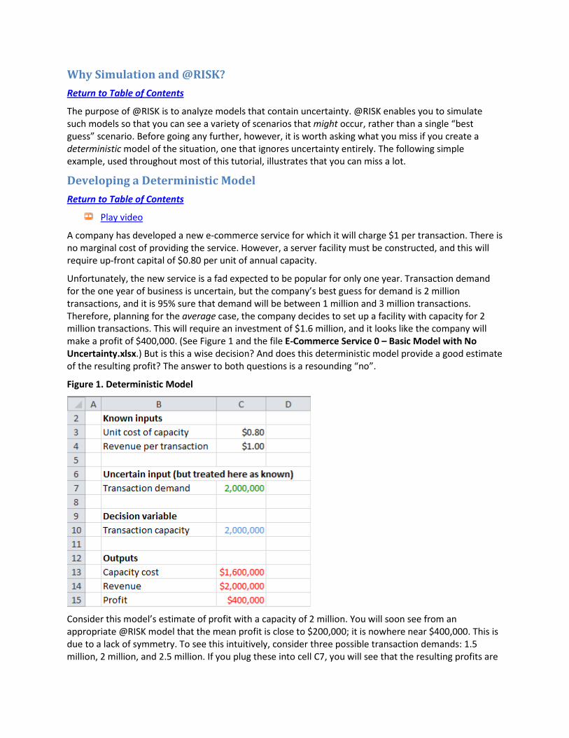
A company has developed a new e-commerce service for which it will charge $1 per transaction. There is no marginal cost of providing the service. However, a server facility must be constructed, and this will require up-front capital of $0.80 per unit of annual capacity.

Unfortunately, the new service is a fad expected to be popular for only one year. Transaction demand for the one year of business is uncertain, but the company’s best guess for demand is 2 million transactions, and it is 95% sure that demand will be between 1 million and 3 million transactions. Therefore, planning for the average case, the company decides to set up a facility with capacity for 2 million transactions. This will require an investment of $1.6 million, and it looks like the company will make a profit of $400,000. (See Figure 1 and the file E-Commerce Service 0 – Basic Model with No Uncertainty.xlsx.) But is this a wise decision? And does this deterministic model provide a good estimate of the resulting profit? The answer to both questions is a resounding “no”.

Figure 1. Deterministic Model

Consider this model’s estimate of profit with a capacity of 2 million. You will soon see from an appropriate @RISK model that the mean profit is close to $200,000; it is nowhere near $400,000. This is due to a lack of symmetry. To see this intuitively, consider three possible transaction demands: 1.5 million, 2 million, and 2.5 million. If you plug these into cell C7, you will see that the resulting profits are

–$100,000 (a loss), $400,000, and $400,000. The reason is that your revenue decreases by $1 for every transaction below 2 million, but it cannot increase for transactions above 2 million because you don’t have the capacity to service them. Therefore, the most profit you can make with this capacity is $400,000—and your actual profit can be a lot less than this. Hence, the deterministic profit model is very misleading in terms of the profit you are likely to make. For the same basic reason, setting capacity below the most likely number of transaction demand (2 million) turns out to a much better decision, as you will soon see.

The point here is that if you have a situation with a fair amount of uncertainty, you should view a deterministic model, even one with good guesses for the uncertain inputs, with a lot of skepticism. You will capture reality much better—and you will learn a lot more about this reality—if you treat the uncertainty explicitly. Fortunately, this is exactly what @RISK enables you to do. It lets you build simulation models that explicitly incorporate uncertainty.

Overview of @RISK Return to Table of Contents

Any Excel model, simulation or otherwise, contains the following elements:

• Known inputs to the model (the “given” values such as unit price and unit cost) • Uncertain inputs (such as transaction demand) • Outputs (one or more “bottom line” values such as total cost and profit) • Formulas that contain the logic for calculating outputs from inputs

People use the term “input” in various ways. In a general Excel model, inputs are any known numbers that you start with. Through Excel formulas, these inputs lead to outputs of interest. The situation is slightly more complicated with @RISK models. Some of the inputs are known values and others are uncertain and require probability distributions. In its various dialog boxes and reports, @RISK uses the term “input” to refer only to the uncertain inputs, not the known values. This might be confusing, so in this tutorial, the terms “known inputs” and “uncertain inputs” are used instead. The former are known values, and the latter require probability distributions. Actually, these probability distributions usually require “parameters,” such as the mean and standard deviation of a normal distribution. These parameters will be clearly marked as such in this tutorial.

Many Excel models also include one or more decision variables, values that can be changed to make certain outputs move in the desired direction. For example, a company might need to choose an order quantity for its product to maximize its expected profit. Finally, an important byproduct of most Excel models is that they facilitate sensitivity analysis, where you can see how various outputs vary as inputs and/or decision variables are varied in a systematic way.

@RISK models have all of these features, so if you are comfortable building and using Excel models, you should have no trouble with @RISK. You still have to decide what the known inputs, the uncertain inputs, and possibly the decision variables are, what outputs you want to keep track of, and how to relate them with appropriate formulas. However, the big difference in @RISK models is that the uncertain inputs are modeled with probability distributions.

When you run an @RISK simulation model, you actually recalculate many iterations of it. On each iteration, @RISK samples a random value from each cell containing a probability distribution, that is, from each uncertain input, recalculates the model with the sampled values, and keeps track of the output values for that iteration. After all iterations have been performed, it shows you the results, both in graphical and numerical form. For example, if profit is an output, it shows you the smallest profit in

any of the iterations, the largest profit in any of the iterations, the mean (average) profit over all iterations, the standard deviation of profit over all iterations, a histogram of these profits, and much more. Fortunately, @RISK takes care of many of the tedious details, allowing you time to carefully examine the resulting distribution of profit. In addition, if you have one or more decision variables, @RISK enables you to vary their values in a systematic way, so that you can see which value(s) leads to the “best” output values.

Opening and Closing @RISK Return to Table of Contents

Before you can use @RISK, you must load it into memory. This is easy. It can be done with Excel already open, or it can be done with Excel not yet open. In the latter case, opening @RISK opens both Excel and @RISK.

You can simply launch @RISK from the desktop icon if you elected to place it there during installation, or you can go to the Windows Start button, find the Palisade Decision Tools group in the list of all Programs, and select @RISK. It usually takes a few seconds for @RISK to load, and you will eventually see an @RISK welcome window. Once you close this window, you will know that @RISK is loaded because you will see an @RISK tab for its ribbon in Excel 2007 and 2010. (@RISK is also compatible with Excel 2000-2003, where it adds a new toolbar.)

To unload @RISK from memory, you have two choices. If you close Excel, @RISK will close as well. Alternatively, you can click the Utilities dropdown in the Tools group of the @RISK ribbon and select Unload @RISK Add-In. This unloads @RISK but keeps Excel open.

Steps for Developing an @RISK Model Return to Table of Contents

Most @RISK models are developed with the same basic steps. For reference, these steps are listed here and are then explained and implemented in the following sections.

1. Decide which inputs are known with a fair amount of certainty and which inputs are uncertain. The latter should be modeled with probability distributions, as explained in the previous section.

2. Decide which probability distributions to use for the uncertain inputs. Some general guidelines for doing this will be given shortly.

3. Determine the decision variables, if any, in the model, and provide “reasonable” values for them. You can use several @RISK tools to find better values for these decision variables, as discussed in step 10.

4. Create an Excel model in the usual way, using appropriate Excel formulas to implement the logic that leads from the known inputs, the uncertain inputs, and the decision variables to outputs. This step is often the most difficult and time-consuming step in the process, depending on the complexity of the model, but it has nothing specifically to do with @RISK. It requires the usual Excel logic.

5. Designate the output(s) you want @RISK to keep track of. You can have a single designated output, or you can have many. It all depends on what you want to keep track of.

6. Change @RISK settings as necessary, especially the number of iterations and possibly the number of simulations.

7. Run the simulation. 8. Examine the distributions of the designated outputs with various @RISK tables and charts.

9. Perform sensitivity analysis on the results to see which of the uncertain inputs have the largest effects on the outputs.

10. If there are decision variables, use @RISK to find “good” values for them.

@RISK User Interface Return to Table of Contents

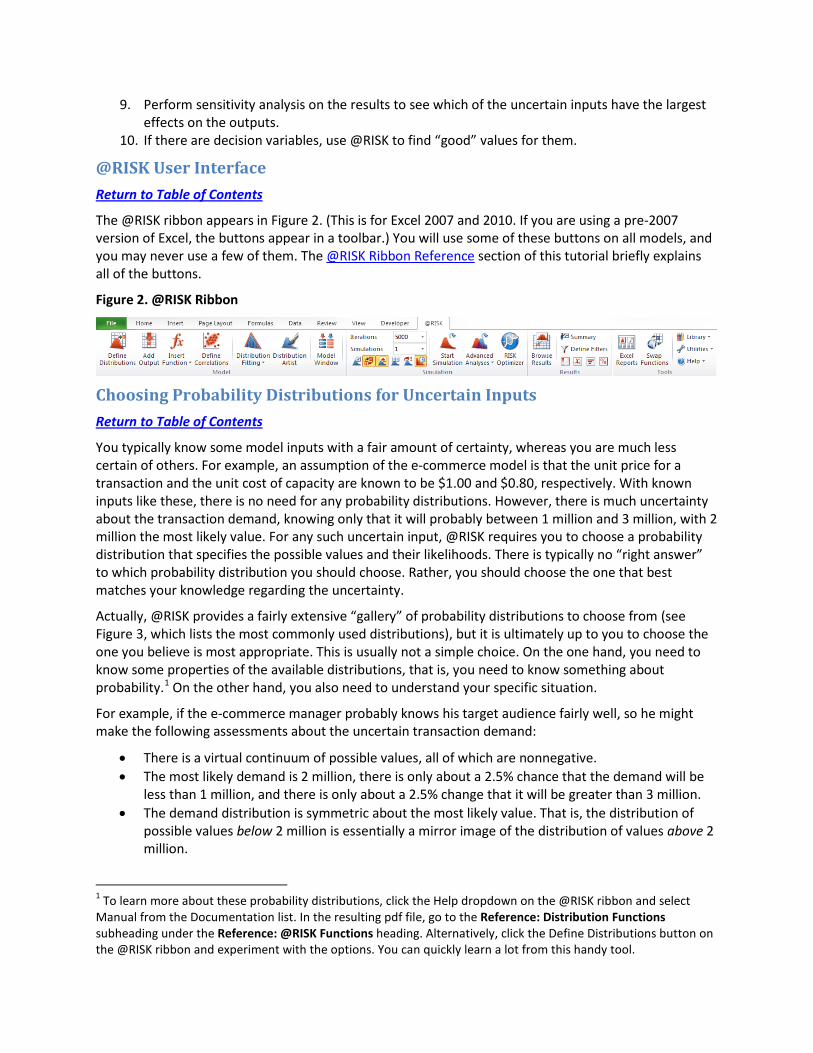
The @RISK ribbon appears in Figure 2. (This is for Excel 2007 and 2010. If you are using a pre-2007 version of Excel, the buttons appear in a toolbar.) You will use some of these buttons on all models, and you may never use a few of them. The @RISK Ribbon Reference section of this tutorial briefly explains all of the buttons.

Figure 2. @RISK Ribbon

Choosing Probability Distributions for Uncertain Inputs Return to Table of Contents

You typically know some model inputs with a fair amount of certainty, whereas you are much less certain of others. For example, an assumption of the e-commerce model is that the unit price for a transaction and the unit cost of capacity are known to be $1.00 and $0.80, respectively. With known inputs like these, there is no need for any probability distributions. However, there is much uncertainty about the transaction demand, knowing only that it will probably between 1 million and 3 million, with 2 million the most likely value. For any such uncertain input, @RISK requires you to choose a probability distribution that specifies the possible values and their likelihoods. There is typically no “right answer” to which probability distribution you should choose. Rather, you should choose the one that best matches your knowledge regarding the uncertainty.

Actually, @RISK provides a fairly extensive “gallery” of probability distributions to choose from (see Figure 3, which lists the most commonly used distributions), but it is ultimately up to you to choose the one you believe is most appropriate. This is usually not a simple choice. On the one hand, you need to know some properties of the available distributions, that is, you need to know something about probability.1 On the other hand, you also need to understand your specific situation.

For example, if the e-commerce manager probably knows his target audience fairly well, so he might make the following assessments about the uncertain transaction demand:

• There is a virtual continuum of possible values, all of which are nonnegative. • The most likely demand is 2 million, there is only about a 2.5% chance that the demand will be

less than 1 million, and there is only about a 2.5% change that it will be greater than 3 million. • The demand distribution is symmetric about the most likely value. That is, the distribution of

possible values below 2 million is essentially a mirror image of the distribution of values above 2 million.

1 To learn more about these probability distributions, click the Help dropdown on the @RISK ribbon and select Manual from the Documentation list. In the resulting pdf file, go to the Reference: Distribution Functions subheading under the Reference: @RISK Functions heading. Alternatively, click the Define Distributions button on the @RISK ribbon and experiment with the options. You can quickly learn a lot from this handy tool.

Figure 3. Common Probability Distributions

These assessments typically come from talking with domain experts, reading relevant reports, and hard thinking about the specific uncertain inputs at hand. But once these assessments are made, they lead naturally to one or more candidate probability distributions from @RISK’s gallery. In the current example, the normal distribution is a reasonable choice, as are the beta general and the symmetric triangular distributions shown in Figure 3. For the sake of discussion, the normal distribution will be used from here on. Furthermore, because there is about a 95% chance of being within two standard deviations of the mean for a normal distribution, the assessments imply that the appropriate normal distribution has mean 2 million and standard deviation 0.5 million.2

The normal distribution has been chosen in this example partly because it is the most familiar distribution to most people. However, you should not fall into the trap of using the normal distribution for every uncertain input in every @RISK model. You should check whether the bulleted assumptions above are reasonable. Assessments that would lead you to a non-normal distribution are quite common and include the following:

• The uncertain input is bounded above and below by natural limits. An example is the quality of a manufactured product, measured on a 0–100 scale.

• The uncertain input can have only a few integer values. An example is the number of accidents a driver has in a given year. In this case, a discrete distribution should be used.

• The distribution of the uncertain input is definitely skewed, not symmetric. An example is the time until burnout of a light bulb, where times much greater than the most likely time are certainly possible, but times much less than the most likely time are not possible.

2 Note that this normal distribution has some possible negative values, and a negative value makes no sense for a demand. However, with mean 2 million and standard deviation 0.5, there is very little probability of a negative value occurring. If this is a concern, perhaps the normal distribution should not be chosen. Alternatively, @RISK provides the option of a normal distribution truncated at 0, which eliminates the possibility of negative values.

This is why there are so many probability distributions in the @RISK gallery. Some are bounded; some are open-ended. Some are continuous; some are discrete. Some are symmetric; some are skewed in one direction or the other. The more of these distributions you know, the more likely you will be able to choose one that is appropriate for your situation. Just remember that the input probability distribution(s) you use in your @RISK models can make a difference in terms of the resulting outputs, so you should spend the time to choose them carefully.

Sometimes you have historical data that can lead you to the appropriate distribution for some uncertain input. For example, you might need future stock price changes for some model. If you have a lot of past price changes for the same stock, you could look at the distribution of these and use it to estimate the distribution of future price changes. @RISK has a fitting tool to help you find the best fit. It is discussed in the Fitting Distributions to Data section of this tutorial.

Developing and Analyzing an @RISK Simulation Model Return to Table of Contents

Play video

Now you get a chance to develop an @RISK model and analyze it. This will build upon the deterministic e-commerce model discussed earlier. You can either open the E-Commerce Service 1 - Basic @RISK Model.xlsx file, or you can start with a blank worksheet and fill it in according to the instructions given below. For reference, the completed model appears in Figures 4 (which shows values) and 5 (which shows formulas). The instructions here follow the same steps as in the previous section.

1. There are two known inputs, the unit cost of capacity and the revenue per transaction, and there is one unknown input, transaction demand. The known inputs are assumed to be $0.80 and $1.00, respectively. The transaction demand is modeled with a probability distribution.

2. For reasons discussed earlier, the selected probability distribution for transaction demand is normal with mean 2 million and standard deviation 0.5 million. To use this probability distribution, enter the formula =RISKNORMAL(F7,G7) in cell C7.3 The RISKNORMAL function takes a mean and standard deviation as parameters. All @RISK probability functions start with RISK, followed by the name of the distribution and any relevant parameters. An easy way to enter any such distribution (if you don’t want to type it) is to select a blank cell, click the Define Distributions button on the @RISK ribbon, select the distribution of interest, such as normal, enter its parameters, and click OK. This pastes the correct formula into the cell. Now press the F9 key a few times to recalculate. You will see that the transaction demand changes randomly, and all cells that depend on it also change. This is the essence of simulation. However, if nothing happens when you press the F9 key, you need to change an @RISK setting. In the middle of the @RISK ribbon, there is a “dice” toggle button that can be orange or white. When it is orange, cells with uncertain inputs change value randomly when you press the F9 key. This is probably the setting you will want in your @RISK models. However, if you want to see the results of a model with all uncertain inputs set equal to their means, toggle the dice button to white. This can be very useful for comparing a model with uncertainty to a model with the uncertainty removed.

3 This tutorial capitalizes all @RISK (and other Excel) functions for emphasis, but they are not case sensitive.

3. There is one decision variable in the model, capacity. Enter any reasonable value for it in cell C10. The value 2 million is used here, but it will be varied in step 10.

Figure 4. E-Commerce Simulation Model

4. The logic for this model is quite straightforward and is developed with the formulas in cells C13

to C15. (See Figure 5.) Specifically, the formula in cell C14 indicates that the company can sell only the smaller of transaction demand and transaction capacity.

5. Any of cells C13 to C15 could be of interest as an output, but only the profit in cell C15 will be designated as such. To do so, select this cell and click the Add Output button on the @RISK ribbon. @RISK appends RISKOUTPUT()+ to the formula in cell C15. Note, however, that this does not indicate addition. It is simply @RISK’s way of indicating that it will keep track of the values in this cell. If you wanted the revenue cell (or any other cell) to be an @RISK output cell as well, you could select it and again click the Add Output button.

Figure 5. Formulas for E-Commerce Model

6. There are many @RISK settings you can change, but you will typically change only the number of

iterations and possibly the number of simulations (more about the latter in step 10). For now, choose 5000 as the number of iterations and the number of simulations to be 1. In general, the more iterations you choose, the more accurate the results will be. The only downside to a large number of iterations is increased computing time. Usually, a value from 1000 to 5000 suffices.

7. To run the simulation, click the Start Simulation button on the @RISK ribbon. You will see the progress at the lower left of the screen. The run time depends entirely on the complexity of the model and the speed of your PC, but you typically won’t need to wait very long. (Note: To speed up the progress, it is best to have only one @RISK model open at a time. If several are open, they will all recalculate at the same time, and this can be a significant drag on speed.)

8. By this time, @RISK has stored 5000 scenarios in memory (or however many iterations you requested), and you can now analyze the results. Because this is such an important part of the overall procedure, @RISK provides a number of ways to see the results, and you will undoubtedly develop your favorites. They include the following:

a. To see a quick histogram of any designated output, select the output cell and click the Browse Results button on the @RISK ribbon.4 The histogram of profit for a capacity of 2 million appears in Figure 6. This chart is interactive, meaning that you can drag the vertical slider bars to find various percentiles or probabilities. And don’t be afraid to experiment with the various buttons at the bottom of the window. Does this histogram surprise you, given the normal (bell-shaped) distribution of demand? It shouldn’t. The extreme skewness is due to the asymmetry in the model, as discussed earlier. If transaction demand is at least 2 million, profit is always $400,000. This explains the large spike to the right. But as transaction demand decreases from 2 million, profit gradually decreases. This explains the long tail to the left. The summary measures listed on the right (such as mean profit of about $200,000) are important, but the shape of the histogram provides the most insight.

Figure 6. Histogram of Profit from Browse Results5

b. To see a quick summary of any output, click the Summary button on the @RISK window.

This leads to the results in Figure 7. If there were multiple outputs, you would see all of them. This window is actually interactive. If you right-click any output and select Columns for Table, you can choose the summary measures you want to appear. And, as

4 Actually, this histogram might already be visible, depending on which cell is active when you run the simulation. However, if you turn off Live Update, which can save computing time, the histogram will not be visible until after the simulation is run. 5 The screenshots in this tutorial are from @RISK 6.0. They differ slightly from those in version 5.7. For example, the Browse Results window now has many more statistics listed in the right pane.

with the Browse Results window, don’t be afraid to experiment with the buttons at the bottom of the window. (Note: If you drag a thumbnail graph in the Summary Window to the worksheet, you get an interactive chart, exactly as if you had clicked the Browse Results button for that output.)

Figure 7. Summary Window for Profit

c. If you want to see summary measures of an output in cells on the same worksheet as the model, you can use a number of @RISK statistical functions. These include RISKMEAN, RISKSTDDEV, RISKPERCENTILE, RISKTARGET, and a few others.6 Several of these appear in Figures 4 and 5 in rows 18–24. All of these summarize the 5000 values of profit that were generated by the simulation. Therefore, these cells are meaningless until you run the simulation, so don’t worry if you see crazy numbers or even errors in these cells. Just run the simulation to make them come alive. Note that a formula such as =RISKTARGET(C15,0) returns the fraction of iterations where profit is less than or equal to the second argument. If you want a “greater than” fraction, you can subtract RISKTARGET from 1.

d. The Browse Results and Summary options provide quick but not permanent results; they don’t save with the file.7 If you want permanent versions, click the Excel Reports button on the @RISK ribbon. This gives you a choice of several types of reports. A good choice is Quick Reports, which leads to the results in Figure 8, but you can experiment with the other report types. (Only part of the report is shown here.) Note that by default, these reports are stored in a new workbook, not the workbook that contains your model. If you would rather have the reports in your model’s workbook, click @RISK’s Utilities dropdown, select Application Settings, and change the “Place Reports In” setting to Active Workbook. This setting will “stick” on all future models unless you change it again.

6 To see more of these, click the Insert Function dropdown on the @RISK ribbon and select the Simulation Result group. If you hover your mouse over any function, you will see a quick description of the function. 7 Actually, this isn’t quite true. In either the Browse Results window or the Summary window, one of the buttons at the bottom of the window allows you to store the results in an Excel worksheet.

Figure 8. Quick Reports on Profit

e. For even more results, click either the Simulation Detailed Statistics button or the

Simulation Data button on the @RISK ribbon. The former lists the detailed summary measures (and even more) shown in the bottom right of Figure 8. The latter lists all of the input and output values for each of the iterations. You might not need this level of detail very often, but it is always available. (And remember that “inputs” in @RISK’s windows refer only to the uncertain inputs.)

f. Suppose you want to share the completed model, together with the results, with a colleague who doesn’t own @RISK. You can do this by clicking the Swap Functions button on the @RISK ribbon. This replaces all random functions like RISKNORMAL with their means. If you want to recover the random functions, you can click the Swap Functions a second time.

9. In a typical @RISK model, there are several uncertain inputs and at least one designated output cell. Then the most natural sensitivity analysis is to check which uncertain inputs have the largest effects on a given output. For the current e-commerce model, this is not relevant because there is only one uncertain input. To illustrate how it can be useful, the model was

modified so that the unit cost of capacity and the revenue per transaction, along with transaction demand, are treated as uncertain. (See the file E-Commerce Service 2 – Basic Model with Extra Uncertainty.xlsx.) These quantities are all assumed to be normally distributed with the means and standard deviations indicated in Figure 9. For example, the formula in cell C6 is =RISKNORMAL(F6,G6), and the formulas in cells C7 and C8 are similar. Nothing else in the model has been changed. To see which of the three uncertain inputs has the largest effect on profit, you can run the simulation for 5000 iterations as before. Then, if a chart for profit is not visible, select the profit cell, click the Browse Results button, and click the “tornado” button at the bottom of the window (the 5th button from the left). This creates the tornado chart in Figure 10. It is called a tornado chart because the longest bars are at the top of the chart. The longer the bar, the more effect this uncertain input has on profit. Here, you can see that the transaction demand has the largest (positive) effect on profit, followed by revenue per transaction and (in a negative direction) the unit cost of capacity.8

10. To this point, the capacity has been set to the most likely demand, 2 million. But there is no guarantee that this is the “best” capacity to choose. Fortunately, @RISK has a very handy RISKSIMTABLE function that lets you try several capacities in one large simulation run. From the resulting outputs, you can then choose the one you like best. Figure 11 shows how it is done. (See the file E-Commerce Service 3 – Model with Different Capacities.xlsx for this modified model, which again has only one uncertain input, transaction demand.) You can list any capacities you want to try in row 10 and then enter the formula =RISKSIMTABLE(E10:M10) in cell C10. This cell then displays the first capacity in the list, but all of them are eventually tried. However, you must first change one @RISK setting. You must set the number of simulations to 6, not 1. Each of these will run with the number of iterations specified, such as 5000. And importantly, @RISK uses the same transaction demand values in each of the simulations. This results in a fair comparison. After you run the simulations, you can get results in any of the ways described earlier, but now they are broken down by the simulation number (1 to 6). For example, to see the summary measures in rows 20-26, you can enter the same @RISK statistical functions as before but add the simulation number as a last argument, such as =RISKMEAN($C$15,C18) in cell C20 (where the profit cell is made absolute to enable copying across). Alternatively, you can click Browse Results and right-click the button with the histogram and pound sign (the 5th button from the right) to see a histogram of profit for any of the 6 simulations.

8 If you right-click the tornado button, you will see two choices: regression coefficients or correlation coefficients. Don’t worry too much about this setting; they generally both show similar behavior.

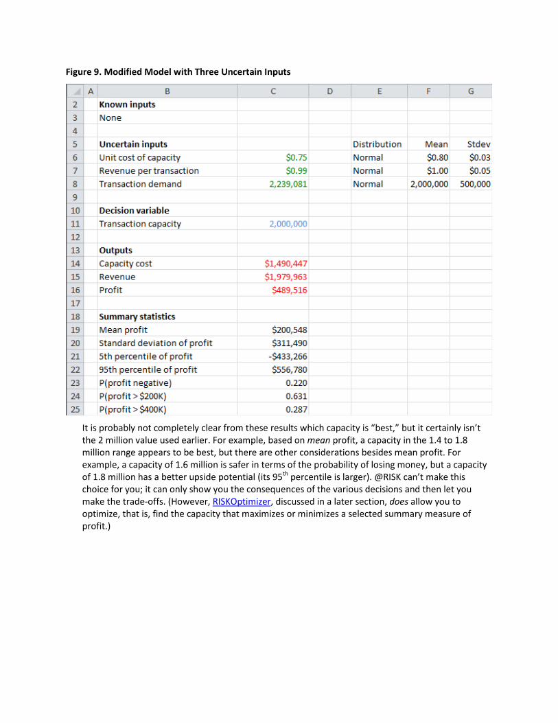
Figure 9. Modified Model with Three Uncertain Inputs

It is probably not completely clear from these results which capacity is “best,” but it certainly isn’t the 2 million value used earlier. For example, based on mean profit, a capacity in the 1.4 to 1.8 million range appears to be best, but there are other considerations besides mean profit. For example, a capacity of 1.6 million is safer in terms of the probability of losing money, but a capacity of 1.8 million has a better upside potential (its 95th percentile is larger). @RISK can’t make this choice for you; it can only show you the consequences of the various decisions and then let you make the trade-offs. (However, RISKOptimizer, discussed in a later section, does allow you to optimize, that is, find the capacity that maximizes or minimizes a selected summary measure of profit.)

Figure 10. Tornado Chart for Profit Sensitivity

Figure 11. Model for Testing Multiple Capacities

More Advanced Features Return to Table of Contents

Play video

If you master everything that has been discussed so far, you will be a very competent and successful @RISK modeler. However, the features described in this section will enable you to step up to an even higher level.

Simulation Settings

Return to Table of Contents

The small Simulation Settings button on the @RISK ribbon opens a dialog box where you can change a lot of advanced settings. For example, the Macros tab enables you to select a macro that should be run during the simulation. You probably won’t need to change any of these advanced settings except for the number of iterations and the number of simulations (and you don’t need the dialog box for these), but there are several other settings you ought to be aware of.

The General tab, shown in Figure 12, provides an alternative way to specify the number of iterations and the number of simulations. It also lets you enable multiple CPU cores in a single machine to speed up simulations. (You are allowed 2 CPUs in the Professional version and an unlimited number in the Industrial version. This setting is enabled by default.)

Figure 12. Random or Static Values

Finally, you can display either random or static values in the uncertain input cells. This setting can be changed, as discussed earlier, by toggling the “dice” button, or it can be changed here. It can be disconcerting to have “random” cells that don’t change when you press the F9 key, so you will probably

want the Random Values setting. On the other hand, the Static Values setting can be very useful when you want to see what the results would be in a deterministic setting, that is, where the uncertainty is removed. Note that the dropdown for Static Values allows four possibilities for static values: expected values, “true” expected values, modes, or percentiles (where you can choose the percentage).9 In any case, be aware that this setting has absolutely no effect when you actually run the simulation.

The Random Numbers section of the Sampling tab, shown in Figure 13, contains some important settings.

• The Sampling Type can be Latin Hypercube or Monte Carlo. Given that spreadsheet simulation is often called Monte Carlo simulation, you might expect Monte Carlo to be the preferred sampling type, but it isn’t. For technical reasons, Latin Hypercube is much more accurate. It is the default @RISK setting, so unless you have a very good reason, you shouldn’t change it.

• The Generator is the method used to generator uniformly distributed random numbers between 0 and 1, the building blocks for random numbers from any distribution. Researchers have developed many random number generators, but the default Mersenne Twister shown here has good statistical properties and is a good choice.

• The Initial Seed can be fixed at any positive integer value, or it can be random. The fixed setting is a good one if you want someone else to replicate your results. If you both use the same seed, you will get identical results. But if you want different results each time you run the simulation, you should use the random option.

• You should keep the “All Use Same Seed” for the Multiple Simulations setting. This provides a fair comparison when you run multiple simulations with a RISKSIMTABLE function.

9 The difference between expected values and “true” expected values is relevant only for discrete inputs. In this case, the “true” expected value can be a value like 13.3. In contrast, the expected value setting would round this to 13. The idea is that if only integer values make sense, a value like 13.3 shouldn’t be used.

Figure 13. Sampling Type

Using Correlated Inputs

Return to Table of Contents

If a model has several uncertain inputs and you enter an @RISK formula such as =RISKNORMAL(100,10) in each of their cells, the uncertain inputs are treated as if they are probabilistically independent. However, quantities in the real world are often correlated to some extent, either positively or negatively. If you know that the uncertain inputs are correlated and you can measure the extent of their correlation, you should account for this correlation in your model by using @RISK’s RISKCORRMAT function. It is usually difficult to gauge how much this actually matters—this depends entirely on the specific model—but there is no excuse for assuming independence when you know it isn’t realistic.

The file Investment Model with Correlated Assets.xlsx illustrates how to do it (see Figure 14). This model assumes you are going to invest certain percentages of your wealth for some period of time (a year, say) in two stocks and a commodity such as gold. The returns are assumed to be normally distributed with the means and standard deviations shown, and they are fairly highly correlated. The two stocks tend to change in the same direction, which tends to be the opposite direction from the commodity (see columns B-E).

Figure 14. Model with Correlated Assets

The quickest way to build this correlation behavior into the model is to first enter the usual RISKNORMAL functions (or whatever distribution you want to use) in the uncertain cells C22 to E22. Then select these cells and click the Define Correlations button on the @RISK ribbon. This opens the dialog box in Figure 15, where you can define a correlation matrix. You give the matrix a name, such as CorrMatrix1, you specify the location for it on the worksheet, and you specify the correlations (actually, only those below the diagonal are required) by typing numbers in the boxes.

Figure 15. Define Correlations Dialog Box

When you click OK, the model appears as in Figure 14, columns B to E. The correlation matrix in rows 15 to 18 has been entered automatically through the Define Correlations dialog box, and rows 28 to 30 indicate how the formulas in cells C22 to E22 have been changed. For example, the original formula in cell C22 was =RISKNORMAL(C11,C12). By adding correlations, you can see that a third argument, RISKCORRMAT(CorrMatrix1,1), has been added to the formula. The last 1 indicates that this is the first

of the three correlated variables. Note that the formulas in cells D22 and E22 have indexes 2 and 3, meaning that they are the second and third correlated variables.

If you prefer, you can skip the Define Correlations dialog box and type the formulas directly, but this will probably take a little more time and increase the chance of making a mistake. Specifically, you can enter the correlations you want directly into cells, range-name the correlation matrix something like CorrMatrix1, and then enter the entire formulas shown in rows 28 to 30 in the uncertain cells.

Note that there are three sets of asset return cells in Figure 14, just for comparison. Those in the middle are for the case of independent returns, so there is no correlation matrix. Those on the right are for the case where the minus signs have been omitted from the correlations; now all returns are positively correlated.

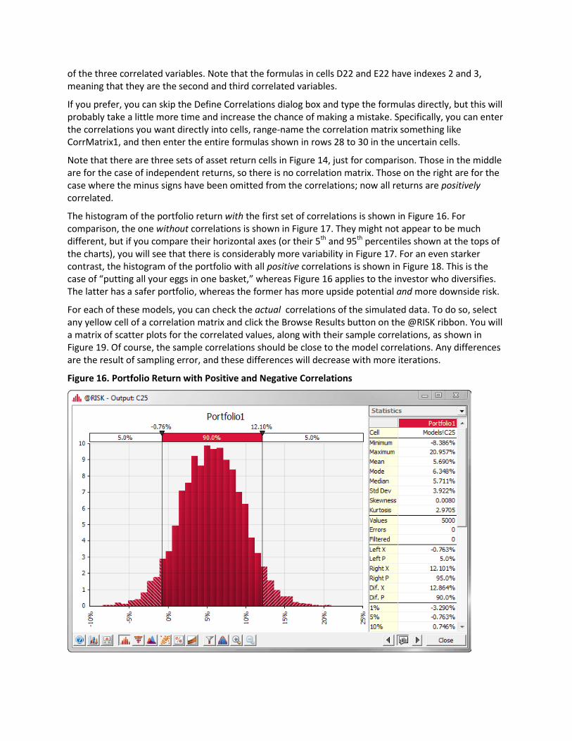
The histogram of the portfolio return with the first set of correlations is shown in Figure 16. For comparison, the one without correlations is shown in Figure 17. They might not appear to be much different, but if you compare their horizontal axes (or their 5th and 95th percentiles shown at the tops of the charts), you will see that there is considerably more variability in Figure 17. For an even starker contrast, the histogram of the portfolio with all positive correlations is shown in Figure 18. This is the case of “putting all your eggs in one basket,” whereas Figure 16 applies to the investor who diversifies. The latter has a safer portfolio, whereas the former has more upside potential and more downside risk.

For each of these models, you can check the actual correlations of the simulated data. To do so, select any yellow cell of a correlation matrix and click the Browse Results button on the @RISK ribbon. You will a matrix of scatter plots for the correlated values, along with their sample correlations, as shown in Figure 19. Of course, the sample correlations should be close to the model correlations. Any differences are the result of sampling error, and these differences will decrease with more iterations.

Figure 16. Portfolio Return with Positive and Negative Correlations

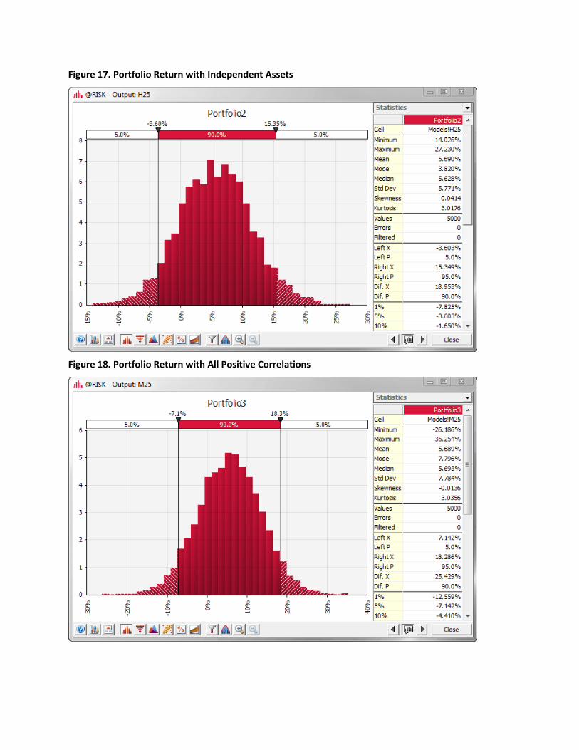
Figure 17. Portfolio Return with Independent Assets

Figure 18. Portfolio Return with All Positive Correlations

Figure 19. Scatter Plots and Sample Correlations

Fitting Distributions to Data

Return to Table of Contents

This tutorial has already discussed the importance of choosing appropriate probability distributions for uncertain inputs, and it has discussed some general principles for doing so. For example, you can sometimes narrow the choice by assessments such as: (1) the quantity must be between 0 and 100; (2) the quantity can have only a few discrete values; or (3) the distribution of the quantity is skewed to the right. Another approach is to fit possible distributions to historical data on the quantity. Of course, historical data are not always available, but when they are, @RISK’s distribution fitting tool can be used. This tool automatically ranks candidate distributions on their goodness-of-fit to the data, and then you can make the ultimate choice of the distribution you want to use.

As an example, the file Fitting a Distribution to Weekly Demands.xlsx contains three years of weekly demands (156 observations) for a company’s product. If a simulation model requires demands in one or more future weeks, it is natural to use a probability distribution that fits the historical data well. To find good fits, click the Distribution Fitting dropdown on the @RISK ribbon and select Fit Distributions to Data.10 In the resulting dialog box, select the data range and the type of data (continuous versus discrete) in the Data tab (see Figure 20), and select candidate distributions you want to try in the Distributions to Fit tab (see Figure 21). Specifically, once you makes some choices about the data in the left side of Figure 21 (for example, lower bound of 0, open upper bound), @RISK automatically checks all the continuous distributions that satisfy these conditions. If you have never heard of some of these distributions, feel free to uncheck them, as was done to a few of them here.

Figure 20. Specifying the Data Range and Type

10 If you have already fit a distribution to the data, you can select Fit Manager from the Distribution Fitting dropdown, and “Goto” any defined data set directly.

Figure 21. Specifying the Candidate Distributions

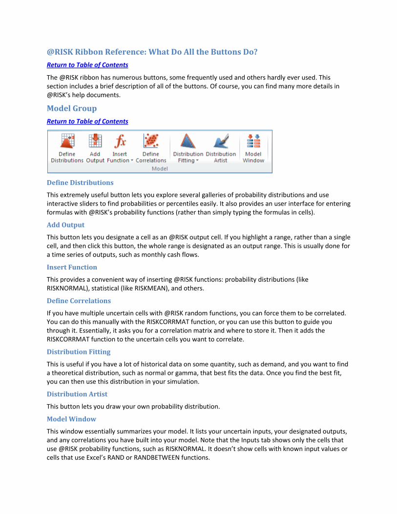
@RISK then fits each of the checked distributions to the data, it ranks them on goodness-to-fit, and it shows you the results graphically and numerically, as in Figure 22. For these data, the best fit (the one with the lowest chi-square value) is the lognormal distribution with parameters 109.34 and 84.071.11 You can see this fit in the graph, where the red curve is the lognormal distribution and the blue bars represent the histogram of the data. By clicking the other distributions in the left pane, you can see how well they fit the data. For this data set, a Weibull fit is also quite good, but the exponential fit is not nearly as good. At this point, you can enter the formula =RISKLOGNORM(109.34,84.071) into a simulation model as the demand for some future week. Even easier, you can click the Write to Cell button in Figure 22 to enter this formula in the active cell. Either way, you can feel comfortable that you have chosen a reasonable probability distribution for demand.

11 @RISK actually ranks the distributions on three criteria (chi-square, Anderson-Darling, and Kolmogorov-Smirnoff), and the rankings can be slightly different depending on the criterion used. For this data set, the lognormal distribution ranks first on two of the three criteria, but the Weibull ranks first on the Anderson-Darling criterion.

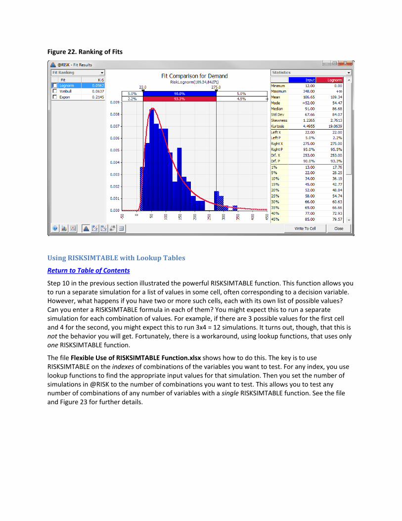
Figure 22. Ranking of Fits

Using RISKSIMTABLE with Lookup Tables

Return to Table of Contents

Step 10 in the previous section illustrated the powerful RISKSIMTABLE function. This function allows you to run a separate simulation for a list of values in some cell, often corresponding to a decision variable. However, what happens if you have two or more such cells, each with its own list of possible values? Can you enter a RISKSIMTABLE formula in each of them? You might expect this to run a separate simulation for each combination of values. For example, if there are 3 possible values for the first cell and 4 for the second, you might expect this to run 3x4 = 12 simulations. It turns out, though, that this is not the behavior you will get. Fortunately, there is a workaround, using lookup functions, that uses only one RISKSIMTABLE function.

The file Flexible Use of RISKSIMTABLE Function.xlsx shows how to do this. The key is to use RISKSIMTABLE on the indexes of combinations of the variables you want to test. For any index, you use lookup functions to find the appropriate input values for that simulation. Then you set the number of simulations in @RISK to the number of combinations you want to test. This allows you to test any number of combinations of any number of variables with a single RISKSIMTABLE function. See the file and Figure 23 for further details.

Figure 23. Using RISKSIMTABLE and Lookup Functions

Using Goal Seek

Return to Table of Contents

You might be familiar the Goal Seek tool in Excel. It is used for solving one equation in one unknown. Specifically, it allows you to force a formula cell to equal a desired value by varying a selected “changing cell.” For example, in a breakeven model, you might want to find the sales volume required to break even, that is, to force profit to zero. @RISK has a very similar Goal Seek tool, found under the Advanced Analyses dropdown. The difference is that it uses a changing cell to force a summary measure (such as a mean, standard deviation, or percentile) of an output cell to a desired value.

As an example, suppose you want to find the capacity in the earlier e-commerce model that forces the mean profit to $230,000. (Remember that this mean is about $200,000 if the capacity is set to 2 million.) The file E-Commerce Service 4 – Model with Goal Seek.xlsx contains the solution. It is exactly the same model as earlier, starting with a capacity of 2 million. (Any reasonable starting capacity could be used.) To force mean profit to $230,000, select Goal Seek from the Advanced Analyses dropdown and fill in the resulting dialog box as shown in Figure 24. (Remember that cell C10 is transaction capacity and cell C15 is profit.) You can speed up the search by adding lower and upper bounds on capacities to search in the Options dialog box (see Figure 25); the tighter the bounds, the quicker the search. Also, note in this dialog box that only an approximate answer is guaranteed: The mean profit will be within 1% of the value desired. (It might take too long to find a more exact value.)

Figure 24. Main Goal Seek Dialog Box

Figure 25. Additional Goal Seek Parameters

The result of Goal Seek for this example appears in Figure 26. Of course, this doesn’t mean that a capacity of 1,207,650 will always lead to a profit of $230,000. It only implies that this capacity will lead to a mean profit of approximately $230,000. Actually, if you then run @RISK again with this capacity, you will not get a mean return of exactly $230,000, but it will be reasonably close. The discrepancy is due to randomness, not to an error in the model or a bug in the software. In fact, if you run Goal Seek again, it is very possible that it will report a slightly different solution, again because of randomness.

Figure 26. Goal Seek Results

Optimizing with RISKOptimizer

Return to Table of Contents

The RISKSIMTABLE function was used earlier in this tutorial to test several capacities for the e-commerce model so that a “best” capacity could be chosen. @RISK’s RISKOptimizer tool can be used to take this a step further.12 It allows you to maximize or minimize a selected summary measure of any @RISK output cell by varying selected “changing cells.” For example, you could maximize mean profit, minimize the standard deviation of profit, or even maximize the probability making profit greater than $220,000. This tutorial provides only a quick glimpse of RISKOptimizer. It is a very powerful tool, and an entire chapter of a book, or even an entire book, could be devoted to it.

To use RISKOptimizer, you must first set up an optimization model, which has been done in the file E-Commerce Service 5 – Model with Optimal Capacity.xlsx. To do so, click the RISKOptimizer dropdown on the @RISK ribbon and select Model Definition. You then fill out a dialog box similar to the one in Figure 27. You must specify (1) whether to minimize or maximize, (2) an output cell, (3) a summary measure of that output to optimize (and there are a lot of choices), any changing cells (and optional bounds on them), and any other constraints. In this model, the 10th percentile of profit is maximized by letting transaction capacity vary from 1 million to 2 million; there are no other constraints. After you click OK, nothing happens, at least not yet. This just stores the model information. To actually perform the optimization, you need to click the RISKOptimizer dropdown and select Start.

12 RISKOptimizer was, and still is, a separate add-in in Palisade’s DecisionTools Suite. However, it is so closely allied with @RISK that it shows up as a button in the @RISK toolbar (in recent versions of @RISK). Nevertheless, an extra step is still required. When you click the button, you are asked whether you want to load RISKOptimizer. You are also given the option to automatically load it whenever @RISK starts.

Figure 27. RISKOptimizer Model Setup

Note that the results from RISKOptimizer are not immediate. This is because it systematically checks many values of the changing cell(s), and for each such set of values, it runs a simulation. However, as it is running, you see the progress in various ways, including the dialog box in Figure 28.13 Here you can monitor the progress. Specifically, the last two boxes show values of the objective, in this case the 10th percentile of profit. The starting value was -240,781, and it has improved to about 271,155. Often, fairly quick improvements will be made at first, but then they will level off. Once you sense that no significant improvements are being made, you can click the stop button on the bottom right and accept the best solution so far. RISKOptimizer then shows you a summary of the final solution.

In this case, it turns out that the best 10th percentile of profit of 271,826 was achieved with a capacity of 1,359,132, which you can see in the file. However, as with the Goal Seek tool, you shouldn’t be surprised if you run @RISK again with this capacity and get a slightly different 10th percentile of profit. This is due to randomness, not to an error in the model or a bug in the software. In fact, if you run RISKOptimizer again, it is very possible that it will converge to a slightly different solution, again because of randomness.

13 You will also see a blue box pointing to the profit cell with the best value of the objective so far.

Figure 28. Progress Monitor for RISKOptimizer

@RISK Ribbon Reference: What Do All the Buttons Do? Return to Table of Contents

The @RISK ribbon has numerous buttons, some frequently used and others hardly ever used. This section includes a brief description of all of the buttons. Of course, you can find many more details in @RISK’s help documents.

Model Group Return to Table of Contents

Define Distributions

This extremely useful button lets you explore several galleries of probability distributions and use interactive sliders to find probabilities or percentiles easily. It also provides an user interface for entering formulas with @RISK’s probability functions (rather than simply typing the formulas in cells).

Add Output

This button lets you designate a cell as an @RISK output cell. If you highlight a range, rather than a single cell, and then click this button, the whole range is designated as an output range. This is usually done for a time series of outputs, such as monthly cash flows.

Insert Function

This provides a convenient way of inserting @RISK functions: probability distributions (like RISKNORMAL), statistical (like RISKMEAN), and others.

Define Correlations

If you have multiple uncertain cells with @RISK random functions, you can force them to be correlated. You can do this manually with the RISKCORRMAT function, or you can use this button to guide you through it. Essentially, it asks you for a correlation matrix and where to store it. Then it adds the RISKCORRMAT function to the uncertain cells you want to correlate.

Distribution Fitting

This is useful if you have a lot of historical data on some quantity, such as demand, and you want to find a theoretical distribution, such as normal or gamma, that best fits the data. Once you find the best fit, you can then use this distribution in your simulation.

Distribution Artist

This button lets you draw your own probability distribution.

Model Window

This window essentially summarizes your model. It lists your uncertain inputs, your designated outputs, and any correlations you have built into your model. Note that the Inputs tab shows only the cells that use @RISK probability functions, such as RISKNORMAL. It doesn’t show cells with known input values or cells that use Excel’s RAND or RANDBETWEEN functions.

Simulation Group Return to Table of Contents

Iterations

This integer setting indicates the number of runs in each simulation. (Many analysts call these replications or recalculations; Palisade calls them iterations.) On each iteration, new random values for all uncertain inputs are generated, and the corresponding outputs are calculated. Usually, 1000 to 5000 iterations are sufficient to obtain reasonably accurate results, but you can ask for as many as you like. The only downside to a large value is increased computer time, especially for complex simulation models.

Simulations

This integer indicates the number of simulations to run, each with the designated number of iterations. This is almost always used in conjunction with a RISKSIMTABLE function. For example, if you want to try 6 values of an order quantity decision variable, you can use RISKSIMTABLE in the order quantity cell and designate 6 simulations. Note that each simulation is run with the same random numbers. This provides a fairer comparison.

Group of Small Buttons:

From left to right, these are the following.

Simulation Settings

You can change a number of settings with this button, but they are mostly for advanced users.

Random/Static Recalc

This “dice” button is a toggle. You can either show all cells with uncertain inputs at their means or make them look random.14 You will probably prefer the latter, where the dice button is orange. However, this is cosmetic only. When you run the simulation, it will run correctly regardless of the dice button setting.

Automatically Show Output Graph

This is another toggle. If it is on (orange), the output graph for the selected output will display while the simulation runs. If this is annoying, you can turn it off. You can always see the output graphs later on through the Browse Results button.

Automatically Show Summary Results Window

This button is linked to the previous button. They can’t both be on (orange). If this one is on, you automatically see the Summary window.

14 Setting them equal to their means is the default, but there are several other possibilities. See the section on Simulation Settings.

Demo Mode

This button is linked to the previous two buttons. Only one of them can be on (orange). This evidently shows more results as the simulation is running.

Live Update

If this button is on (orange), any windows you see from the previous three buttons will update as the simulation is running. Otherwise, they will update only at the end of the simulation. Turning this off can save some time. (As mentioned above, multiple CPUs can also speed up the simulations.)

Start Simulation

This runs the simulation. Before clicking this button, you should designate your output cell(s) and specify the numbers of iterations and simulations.

Advanced Analyses

There are three options here.

Goal Seek

This is very much like Excel’s Goal Seek tool. You designate a changing cell, an output statistic, and a desired value. Then @RISK keeps running simulations with different values in the changing cell until the output statistic is sufficiently close to the desired value. As an example, the output statistic could be the probability of negative profit, and its desired value could be 0.05.

Stress Analysis

This allows you to control the range that is sampled from an input probability distribution function, enabling you to see how different scenarios affect designated outputs without changing your model.

Advanced Sensitivity Analysis

This lets you see how changes in any input—distributions or known values—affect simulation results.

RISKOptimizer

This is actually a separate add-in in the DecisionTools Suite, but it is so linked to @RISK that it now opens when @RISK is loaded. It is much like Excel’s Solver add-in, where you specify the decision variables (changing cells), an objective to optimize, and optionally, constraints. The objective can be one of many summary measures of an output, such as mean profit (to maximize), standard deviation of profit (to minimize), or probability of negative profit (to minimize). The changing cells are then varied in a systematic way until the objective is sufficiently close to optimal. However, unlike with Solver, which runs on deterministic (non-random) models, a simulation must be run for each set of values in the changing cells. This makes RISKOptimizer somewhat slow, but very powerful.

Results Group Return to Table of Contents

Browse Results

This is a quick way to get results after a simulation has been run. You can select any output cell and click this button to get a histogram and several summary measures. There are numerous buttons below the histogram that you can experiment with. You can also use the sliders to find probabilities or percentiles.

Summary

This is another quick way to get results after a simulation has been run. It shows a mini-histogram and several summary measures for each output (and for each simulation, if there is more than one). Again, there are several buttons at the bottom you can experiment with. For example, you can select the columns for the table if you want more, or different, summary measures to appear.

Define Filters

This lets you filter output values for selected values. For example, you could run a World Series simulation with 10,000 iterations and then filter on the number of games, asking for only 6 or 7. It would then show you the results for the subset of the 10,000 iterations where the series lasted 6 or 7 games.

Group of Small Buttons:

From left to right, these are the following.

Simulation Detailed Statistics

This shows even more summary measures of the outputs than are shown in the Summary window.

Simulation Data

This provides a spreadsheet-like view of the values of all uncertain inputs and designated outputs for all iterations of the simulation. You can them copy and paste these into your Excel workbook if you like.

Simulation Sensitivities

This lets you see how sensitive the outputs are to the uncertain inputs. Probably the most popular tool in this group is the tornado chart. For any selected output, this shows chart a horizontal bar for each uncertain input. The longer the bar, the more this uncertain input affects the output. The longest bars are at the top; hence the name tornado chart.

Simulation Scenarios

Scenario analysis allows you to determine which uncertain inputs contribute significantly towards reaching a goal. For example, you might want to determine which uncertain inputs contribute to exceptionally high sales, or you might want to determine which uncertain inputs contribute to profits below $1,000,000. @RISK allows you to define target scenarios for each output. You might be interested in the highest quartile of values in the Total Sales output, or the value less than 1 million in the Net Profits output. You can enter these values directly in the Scenarios row of the @RISK Scenario Analysis window.

Tools Group Return to Table of Contents

Excel Reports

This button provides a variety of reports that become a permanent part of your workbook. Quick Reports is a good option, but you can experiment with the others.

Swap Functions

This button enables you to swap @RISK functions in and out of your workbooks. This makes it easy to give models to colleagues who do not own @RISK. If your model is changed when @RISK functions are swapped out, @RISK will update the locations and static values of @RISK functions when they are swapped back in.

Library

An @RISK library allows a company to store probability functions or simulation results in a database for later use. Essentially, they become corporate assets, not just “one off” models. The library is stored in a SQL Server database, so a connection to a SQL Server database is required.

Utilities

This dropdown has a number of obvious features, such as allowing you to unload @RISK without closing Excel. Its Application Settings item allows you to change all sorts of @RISK settings (for all @RISK models, not just the current one). For example, this is where you can change where you want your results to be stored. By default, the results (such as those from Excel Reports) are stored in a new workbook. You might want to change this so that they are stored in the Active Workbook.

Help

This button allows you to find loads of useful documentation, including the complete user manual. It is also where you go to activate a license.

PALISADE.COM

Palisade Corporation sales@palisade.com

tel: +1 607 277 8000 800 432 RISK fax: + 1 607 277 8001

Palisade Europe sales@palisade-europe.com

tel: +44 1895 425050 fax: +44 1895 425051 UK: 0800 783 5398 France: 0800 90 80 32 Germany: 0800 181 7449 Spain: 900 93 8916

Palisade Asia-Pacific sales@palisade.com.au

tel: +61 2 9252 5922 1 800 177 101 fax: +61 2 9252 2820

Palisade Latinoamérica www.palisade-lta.com

ventas@palisade.com tel: +1 607 277 8000 fax: + 1 607 277 8001

Palisade Brasil www.palisade-br.com

vendas@palisade.com tel: +55 21 2586 6334 tel: +1 607 277 8000 fax: + 1 607 277 8001

Palisade アジア・パシ フィック東京事務所 sales.jp@palisade.com tel: +81 3 5456 5287

fax: +81 3 5456 5511