Paleogenomics DocumentationRelease 0.1.0

Claudio Ottoni

Feb 26, 2021

CONTENTS

1 Contents 31.1 List of Tools . . . . . . . . . . . . . . . . . . . . . . . . . . . . . . . . . . . . . . . . . . . . . . . 31.2 Quality filtering of reads . . . . . . . . . . . . . . . . . . . . . . . . . . . . . . . . . . . . . . . . . 41.3 Metagenomic screening of shotgun data . . . . . . . . . . . . . . . . . . . . . . . . . . . . . . . . . 71.4 Alignment of reads to a reference genome . . . . . . . . . . . . . . . . . . . . . . . . . . . . . . . . 141.5 Variant calling and visualization . . . . . . . . . . . . . . . . . . . . . . . . . . . . . . . . . . . . . 231.6 Filtering, annotating and combining SNPs . . . . . . . . . . . . . . . . . . . . . . . . . . . . . . . . 251.7 DO-IT-YOURSELF . . . . . . . . . . . . . . . . . . . . . . . . . . . . . . . . . . . . . . . . . . . 301.8 Material from previous courses . . . . . . . . . . . . . . . . . . . . . . . . . . . . . . . . . . . . . 33

i

ii

Paleogenomics Documentation, Release 0.1.0

Welcome to the 3rd edition of the “Physalia Paleogenomics” course, online version 16-20 November 2020.

CONTENTS 1

Paleogenomics Documentation, Release 0.1.0

2 CONTENTS

CHAPTER

ONE

CONTENTS

1.1 List of Tools

Data preprocessing

• AdapterRemoval: https://github.com/MikkelSchubert/adapterremoval

Metagenomics screening of shotgun data

• kraken: https://ccb.jhu.edu/software/kraken/

• kraken2: https://ccb.jhu.edu/software/kraken2/index.shtml

• krona: https://github.com/marbl/Krona/wiki

• braken: https://ccb.jhu.edu/software/bracken/

• metaphlan3: https://github.com/biobakery/MetaPhlAn/wiki/MetaPhlAn-3.0

Reads alignment and variants calling

• bwa: https://github.com/lh3/bwa

• gatk: https://software.broadinstitute.org/gatk/

• samtools: http://www.htslib.org/

• bcftools: http://www.htslib.org/

Filtering and manipulating bam files

• picard: https://broadinstitute.github.io/picard/

• dedup: https://github.com/apeltzer/DeDup

aDNA deamination detection and rescalinghttps://github.com/Amine-Namouchi/snpToolkit

• mapDamage: https://ginolhac.github.io/mapDamage/

Creating summary reports

• fastqc: https://www.bioinformatics.babraham.ac.uk/projects/fastqc/

• Qualimap: http://qualimap.bioinfo.cipf.es/

• BAMStats: http://bamstats.sourceforge.net

• MultiQC: http://multiqc.info/

Integrative genomic viewer

• IGV: http://software.broadinstitute.org/software/igv/

SNPs annotation and post-processing

3

Paleogenomics Documentation, Release 0.1.0

• snpToolkit: https://github.com/Amine-Namouchi/snpToolkit

Phylogeny

• IQ-TREE: http://www.iqtree.org/

• Figtree: http://tree.bio.ed.ac.uk/software/figtree

1.2 Quality filtering of reads

1.2.1 Reads quality control

The reads generated by a sequencing platform are delivered in fastq format. The first step of the analysis of rawsequences is the quality-control. To do that, we will use FastQC, which provides a modular set of analyses that youcan use to have a first impression of whether your data has any problems of which you should be aware before doingany further analysis. To run FastQC type the following command:

fastqc filename.fastq.gz

To analyze multiple fastq files you can run FastQC as follows:

fastqc *.fastq.gz

At the end of the analysis, FastQC generates for each input file a summary report, like in the screenshot below:

4 Chapter 1. Contents

Paleogenomics Documentation, Release 0.1.0

Note:

• You can download the reports of FastQC (and any other file) in your laptop with the command scp (SecureCopy), which allows files to be copied to, from, or between different hosts. It uses ssh for data transfer andprovides the same authentication and same level of security as ssh. For example, to copy from a remote host(our server) to your computer:

scp username@remotehost:/full_path_to_file /some/local/directory

• To copy a folder you need to call the option -r

scp -r username@remotehost:/full_path_to_file /some/local/directory

• If you are using a pem file to connect to the server, you have to use in order to download the files:

scp -i filename.pem -r username@remotehost:/full_path_to_file /some/local/→˓directory

1.2.2 Reads quality filtering

Reads filtering is a crucial step as it will affect all downstream analyses. One of the important things to do is totrim the adapters that were used during the preparation of the genomic libraries. For this step we will use the pro-gram AdapterRemoval, which performs adapter trimming of sequencing reads and subsequent merging (collapse) ofpaired-end reads with negative insert sizes (an overlap between two sequencing reads derived from a single DNAfragment) into a single collapsed read. We will analyse the DNA sequences of an ancient sample sequenced in single-end. With this command, the trimmed reads are written to output_single.truncated.gz, the discardedFASTQ reads are written to output_single.discarded.gz, and settings and summary statistics are written tooutput_single.settings.

AdapterRemoval --file1 filename.fastq.gz --basename filename --minlength 30 --trimns -→˓-trimqualities --gzip

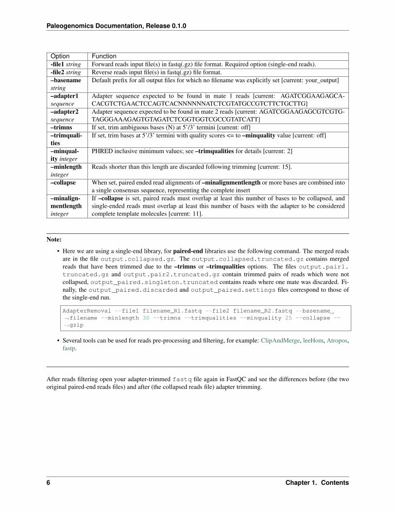
Here some of the options of AdapterRemoval:

1.2. Quality filtering of reads 5

Paleogenomics Documentation, Release 0.1.0

Option Function-file1 string Forward reads input file(s) in fastq(.gz) file format. Required option (single-end reads).-file2 string Reverse reads input file(s) in fastq(.gz) file format.–basenamestring

Default prefix for all output files for which no filename was explicitly set [current: your_output]

–adapter1sequence

Adapter sequence expected to be found in mate 1 reads [current: AGATCGGAAGAGCA-CACGTCTGAACTCCAGTCACNNNNNNATCTCGTATGCCGTCTTCTGCTTG]

–adapter2sequence

Adapter sequence expected to be found in mate 2 reads [current: AGATCGGAAGAGCGTCGTG-TAGGGAAAGAGTGTAGATCTCGGTGGTCGCCGTATCATT]

–trimns If set, trim ambiguous bases (N) at 5’/3’ termini [current: off]–trimquali-ties

If set, trim bases at 5’/3’ termini with quality scores <= to –minquality value [current: off]

–minqual-ity integer

PHRED inclusive minimum values; see –trimqualities for details [current: 2]

–minlengthinteger

Reads shorter than this length are discarded following trimming [current: 15].

–collapse When set, paired ended read alignments of –minalignmentlength or more bases are combined intoa single consensus sequence, representing the complete insert

–minalign-mentlengthinteger

If –collapse is set, paired reads must overlap at least this number of bases to be collapsed, andsingle-ended reads must overlap at least this number of bases with the adapter to be consideredcomplete template molecules [current: 11].

Note:

• Here we are using a single-end library, for paired-end libraries use the following command. The merged readsare in the file output.collapsed.gz. The output.collapsed.truncated.gz contains mergedreads that have been trimmed due to the –trimns or –trimqualities options. The files output.pair1.truncated.gz and output.pair2.truncated.gz contain trimmed pairs of reads which were notcollapsed, output_paired.singleton.truncated contains reads where one mate was discarded. Fi-nally, the output_paired.discarded and output_paired.settings files correspond to those ofthe single-end run.

AdapterRemoval --file1 filename_R1.fastq --file2 filename_R2.fastq --basename→˓filename --minlength 30 --trimns --trimqualities --minquality 25 --collapse --→˓gzip

• Several tools can be used for reads pre-processing and filtering, for example: ClipAndMerge, leeHom, Atropos,fastp.

After reads filtering open your adapter-trimmed fastq file again in FastQC and see the differences before (the twooriginal paired-end reads files) and after (the collapsed reads file) adapter trimming.

6 Chapter 1. Contents

Paleogenomics Documentation, Release 0.1.0

1.3 Metagenomic screening of shotgun data

1.3.1 Kraken 2

In this hands-on session we will use Kraken 2 to screen the metagenomic content of an ancient sample. The firstversion of Kraken (see Kraken) uses a large indexed and sorted list of k-mer/LCA pairs as its database, which may beproblematic for users due to the large memory requirements. For this reason Kraken 2 was developed. Kraken 2 is fastand requires less memory, BUT false positive errors occur in less than 1% of queries (confidence scoring thresholdscan be used to call out to detect them). The default (or standard) database size is 29 GB (as of Jan. 2018, in Kraken 1the standard database is about 200 GB!), and you will need slightly more than that in RAM if you want to build it. Bydefault, Kraken 2 will attempt to use the dustmasker or segmasker programs provided as part of NCBI’s BLAST suiteto mask low-complexity regions.

A Kraken 2 database is a directory containing at least 3 files:

• hash.k2d: Contains the minimizer to taxon mappings

• opts.k2d: Contains information about the options used to build the database

• taxo.k2d: Contains taxonomy information used to build the database

Other files may also be present as part of the database build process, and can, if desired, be removed after a successfulbuild of the database.

Minikraken2

We will first use a pre-built 8 GB Kraken database, called Minikraken2, constructed from complete dusted bacterial,archaeal, and viral genomes in RefSeq. You can download the pre-built Minikraken2 database from the program’swebsite with wget, and extract the archive content with tar:

wget ftp://ftp.ccb.jhu.edu/pub/data/kraken2_dbs/minikraken2_v1_8GB_201904_UPDATE.tgztar -xvzf minikraken2_v1_8GB_201904_UPDATE.tgz

To classify the reads in a fastq file against the Minikraken2 database, you can run this command:

kraken2 --db minikraken2_v1_8GB filename.fastq.gz --gzip-compressed --output filename.→˓kraken --report filename.kraken.report

Some of the options available in Kraken 2:

Option Function–use-names Print scientific names instead of just taxids–gzip-compressed Input is gzip compressed–report <string> Print a report with aggregrate counts/clade to file–threads Number of threads (default: 1)

Note:

• In Kraken 2 you can generate the reports file by typing the --report option (followed by a name for the reportfile to generate) in the command used for the classification.

1.3. Metagenomic screening of shotgun data 7

Paleogenomics Documentation, Release 0.1.0

• In order to run later Krona, the Kraken output file must contain taxids, and not scientific names. So if you wantto run Krona do not call the option --use-names.

The Kraken 2 report format, like Kraken 1, is tab-delimited with one line per taxon. There are six fields, from left toright:

1. Percentage of fragments covered by the clade rooted at this taxon

2. Number of fragments covered by the clade rooted at this taxon

3. Number of fragments assigned directly to this taxon

4. A rank code, indicating (U)nclassified, (R)oot, (D)omain, (K)ingdom, (P)hylum, (C)lass, (O)rder, (F)amily,(G)enus, or (S)pecies. Taxa that are not at any of these 10 ranks have a rank code that is formed by using therank code of the closest ancestor rank with a number indicating the distance from that rank. E.g., “G2” is a rankcode indicating a taxon is between genus and species and the grandparent taxon is at the genus rank.

5. NCBI taxonomic ID number

6. Indented scientific name

Visualization of data with Krona

Finally, we can visualize the results of the Kraken2 analysis with Krona, which disaplys hierarchical data (like tax-onomic assignation) in multi-layerd pie charts. The interactive charts created by Krona are in the html formatand can be viewed with any web browser. We will convert the kraken output in html format using the programktImportTaxonomy, which parses the information relative to the query ID and the taxonomy ID.

ktImportTaxonomy -q 2 -t 3 filename.kraken -o filename.kraken.html

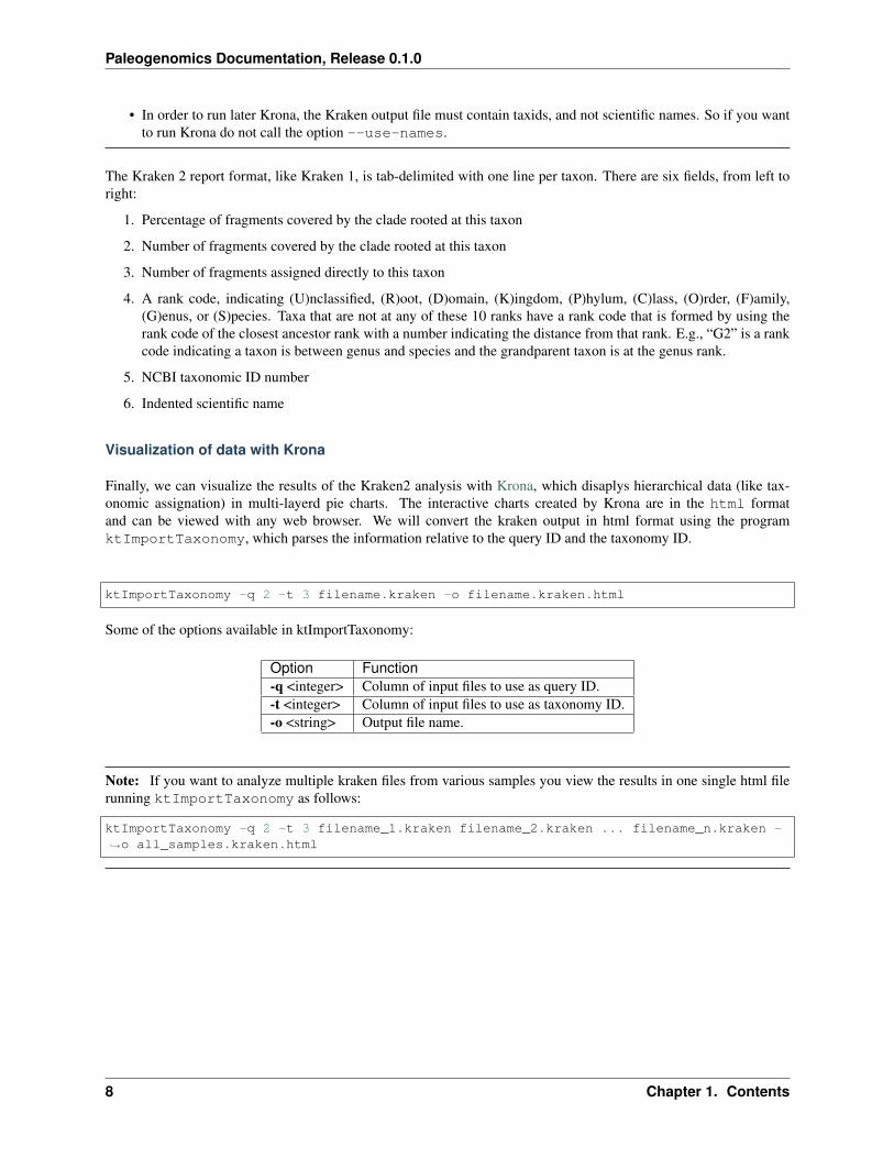
Some of the options available in ktImportTaxonomy:

Option Function-q <integer> Column of input files to use as query ID.-t <integer> Column of input files to use as taxonomy ID.-o <string> Output file name.

Note: If you want to analyze multiple kraken files from various samples you view the results in one single html filerunning ktImportTaxonomy as follows:

ktImportTaxonomy -q 2 -t 3 filename_1.kraken filename_2.kraken ... filename_n.kraken -→˓o all_samples.kraken.html

8 Chapter 1. Contents

Paleogenomics Documentation, Release 0.1.0

Kraken 2 Custom Database

We have already created a custom database to use in this hands-on session so we can go straight to the classification(step 4). However, we report here all the commands to build a Kraken2 database (steps 1-3).

1. The first step is to create a new folder that will contain your custom database (choose an appropriate name forthe folder-database, here we will call it CustomDB). Then we have to install a taxonomy. Usually, you will usethe NCBI taxonomy. The following command will download in the folder /taxonomy the accession numberto taxon maps, as well as the taxonomic name and tree information from NCBI:

kraken2-build --download-taxonomy --db CustomDB

2. Install one or more reference libraries. Several sets of standard genomes (or proteins) are available, which areconstantly updated (see also the Kraken website).

• archaea: RefSeq complete archaeal genomes/proteins

• bacteria: RefSeq complete bacterial genomes/proteins

• plasmid: RefSeq plasmid nucleotide/protein sequences

• viral: RefSeq complete viral genomes/proteins

• human: GRCh38 human genome/proteins

• fungi: RefSeq complete fungal genomes/proteins

• plant: RefSeq complete plant genomes/proteins

• protozoa: RefSeq complete protozoan genomes/proteins

• nr: NCBI non-redundant protein database

• nt: NCBI non-redundant nucleotide database

1.3. Metagenomic screening of shotgun data 9

Paleogenomics Documentation, Release 0.1.0

• env_nr: NCBI non-redundant protein database with sequences from large environmental se-quencing projects

• env_nt: NCBI non-redundant nucleotide database with sequences from large environmental se-quencing projects

• UniVec: NCBI-supplied database of vector, adapter, linker, and primer sequences that may becontaminating sequencing projects and/or assemblies

• UniVec_Core: A subset of UniVec chosen to minimize false positive hits to the vector database

You can select as many libraries as you want and run the following command, which will download the referencesequences in the folder /library, as follows:

kraken2-build --download-library bacteria --db CustomDBkraken2-build --download-library viral --db CustomDBkraken2-build --download-library plasmid --db CustomDBkraken2-build --download-library fungi --db CustomDB

In a custom database, you can add as many fasta sequences as you like. For exmaple, you can download theorganelle genomes in fasta files from the RefSeq website with the commands wget:

wget ftp://ftp.ncbi.nlm.nih.gov/refseq/release/mitochondrion/mitochondrion.1.1.→˓genomic.fna.gzwget ftp://ftp.ncbi.nlm.nih.gov/refseq/release/mitochondrion/mitochondrion.2.1.→˓genomic.fna.gz

The downloaded files are in compressed in the gz format. To unzip them run the gunzip command:

gunzip mitochondrion.1.1.genomic.fna.gzgunzip mitochondrion.2.1.genomic.fna.gz

Then you can add the fasta files to your library, as follows:

kraken2-build --add-to-library mitochondrion.1.1.genomic.fna --db CustomDBkraken2-build --add-to-library mitochondrion.2.1.genomic.fna --db CustomDB

3. Once your library is finalized, you need to build the database (here we set a maximum database size of 8 GB(you must indicate it in bytes!) with the --max-db-size option).

kraken2-build --build --max-db-size 8000000000 --db CustomDB

Warning: Kraken 2 uses two programs to perform low-complexity sequence masking, both availablefrom NCBI: dustmasker, for nucleotide sequences, and segmasker, for amino acid sequences. Theseprograms are available as part of the NCBI BLAST+ suite. If these programs are not installed on the localsystem and in the user’s PATH when trying to use kraken2-build, the database build will fail. Users whodo not wish to install these programs can use the --no-masking option to kraken2-build in conjunctionwith any of the --download-library, --add-to-library, or --standard options; use of the--no-masking option will skip masking of low-complexity sequences during the build of the Kraken 2database.

The kraken2-inspect script allows users to gain information about the content of a Kraken 2 database.You can pipe the command to head, or less.

10 Chapter 1. Contents

Paleogenomics Documentation, Release 0.1.0

kraken2-inspect --db path/to/dbfolder | head -5

4. Finally, we can run the classification of the reads against the custom database with the kraken2 command:

kraken2 --db CustomDB filename.fastq.gz --gzip-compressed --output filename.→˓kraken --report filename.report

5. To visualize the results of the classification in multi-layerd pie charts, use Krona, as described in the section3.1.2: Visualization of data with Krona

Note: Recently, a novel metagenomics classifier, KrakenUniq, has been developed to reduce false-positive identifi-cations in metagenomic classification. KrakenUniq combines the fast k-mer-based classification of Kraken with anefficient algorithm for assessing the coverage of unique k-mers found in each species in a dataset. On various testdatasets, KrakenUniq gives better recall and precision than other methods and effectively classifies and distinguishespathogens with low abundance from false positives in infectious disease samples.

1.3.2 Bracken

Kraken and Kraken 2 classify reads to the best matching location in the taxonomic tree, but they do not estimateabundances of species. To do that we will use Bracken (Bayesian Reestimation of Abundance with KrakEN), whichestimates the number of reads originating from each species present in a sample. Bracken computes probabilities thatdescribe how much sequence from each genome in the Kraken database is identical to other genomes in the database,and combine this information with the assignments for a particular sample to estimate abundance at the species level,the genus level, or above. Bracken is compatible with both Kraken 1 and Kraken 2 (just note that the default kmerlength is different, 31 in Kraken, 35 in Kraken 2).

Bracken from Minikraken 2

Prior to abundance estimation with Bracken, each reference genome contained in the Kraken database is divided into“read-length kmers”, and each of these read-length kmers are classified. To do that, we need the library and taxonomyfolders of the kraken database that we used for classification. This will generate a kmer distribution file, for examplesfor read-length kmers of 100 nucleotides: database100mers.kmer_distrib. The kmer distribution file willbe used for the following bracken analysis. As pre-built database, Minikraken already contains three kmer distributionfiles built at 100, 150, 200 kmers.

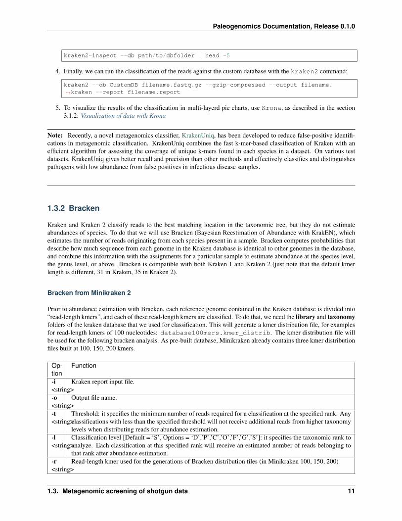
Op-tion

Function

-i<string>

Kraken report input file.

-o<string>

Output file name.

-t<string>

Threshold: it specifies the minimum number of reads required for a classification at the specified rank. Anyclassifications with less than the specified threshold will not receive additional reads from higher taxonomylevels when distributing reads for abundance estimation.

-l<string>

Classification level [Default = ‘S’, Options = ‘D’,’P’,’C’,’O’,’F’,’G’,’S’]: it specifies the taxonomic rank toanalyze. Each classification at this specified rank will receive an estimated number of reads belonging tothat rank after abundance estimation.

-r<string>

Read-length kmer used for the generations of Bracken distribution files (in Minikraken 100, 150, 200)

1.3. Metagenomic screening of shotgun data 11

Paleogenomics Documentation, Release 0.1.0

To run Bracken on one sample we use the following command, with a threshold set at 10, and the read length set at100 (so as to use the database100mers.kmer_distrib file inside the minikraken2_v1_8GB folder):

bracken -d path/to/minikraken2_v1_8GB -i sample.kraken.report -o sample.bracken -r→˓100 -t 10

To speed the process, we can also use variables to set up the options and the paths to the minikraken database and otherfolders, and a for loop. We will generate taxonomic abundances at the species level (the default option). Rememberto create first an output folder (with mkdir). Also note that you can set as path variables either relative paths (basedon your actual position and path) or absolute paths:

KRAKEN_DB=/path/to/kraken/db-folderOUTPUT=/path/to/output-folderREAD_LEN=100THRESHOLD=10

for i in $(find -name "*krk.report" -type f)do

FILENAME=$(basename "$i")SAMPLE=${FILENAME%.krk.report}bracken -d $KRAKEN_DB -i $i -o $OUTPUT/${SAMPLE}.bracken -r $READ_LEN -t $THRESHOLD

done

The Bracken output file is tab-delimited. There are seven fields, from left to right:

1. Name

2. Taxonomy ID

3. Level ID (S=Species, G=Genus, O=Order, F=Family, P=Phylum, K=Kingdom)

4. Kraken Assigned Reads

5. Added Reads with Abundance Reestimation

6. Total Reads after Abundance Reestimation

7. Fraction of Total Reads

Bracken from Custom databases

The Minikraken database is available with all the files needed to run Bracken. If you used a custom database you mustgenerate yourself the kmer_distrib file and the other Bracken database files with bracken-build. To do that,we need the library and taxonomy folders of the kraken database that we used for classification. These are big sizefolders, but do not delete them if you plan to generate Braken databases in the future at different “read-length kmers”.You can select the “read-length kmers” that is most suitable for your samples (namely the average insert size of yourlibrary, e.g. 60 bp for ancient libraries). You can also generate several kmer_distrib files and make different runs(as in Minikraken run, where 100, 150 and 200 are available). You can find all the steps for generating the Brackendatabase files in the Bracken manual.

12 Chapter 1. Contents

Paleogenomics Documentation, Release 0.1.0

1.3.3 Mataphlan 3

MetaPhlAn is a computational tool that relies on ~1.1M unique clade-specific marker genes identified from ~100,000reference genomes (~99,500 bacterial and archaeal and ~500 eukaryotic) to conduct taxonomic profiling of microbialcommunities (Bacteria, Archaea and Eukaryotes) from metagenomic shotgun sequencing data. MetaPhlAn allows:

• unambiguous taxonomic assignments;

• an accurate estimation of organismal relative abundance;

• species-level resolution for bacteria, archaea, eukaryotes, and viruses;

• strain identification and tracking

• orders of magnitude speedups compared to existing methods.

• metagenomic strain-level population genomics

We are not going to cover to in detail MetaPhlAn, but this is a great tool given its specificity, in particular to confirmthe detection of peculiar microbial species (e.g. pathogens).

Warning: Please note that MetaPhlAn may have been installed in a separate environment that we calledmetaphlan. In that case, if you are already working in a conda environment, get out of it with condadeactivate, and activate the metaphlan environment conda activate metaphlan.

The basic usage of MetaPhlAn for taxonomic profiling is:

metaphlan filename.fastq(.gz) --input_type fastq -o outfile.txt

Note: MetaPhlAn relies on BowTie2 to map reads against marker genes. To save the intermediate BowTie2 outputuse --bowtie2out, and for multiple CPUs (if available) use --nproc:

metaphlan filename.fastq(.gz) --bowtie2out filename.bowtie2.bz2 --nproc 5 --input_→˓type fastq -o output.txt

The intermediate BowTie2 output files can be used to run MetaPhlAn quickly by specifying the input(--input_type bowtie2out):

metaphlan filename.bowtie2.bz2 --nproc 5 --input_type bowtie2out -o output.txt

For more information and advanced usage of MetaPhlAn see the manual and the wiki page. And, recently, MetaPhlAn3 has been released!

1.3.4 Other tools

We remind you that there are several metagenomic classifiers, all with their pros and cons, as discussed in the lecture.Other tools that we want to suggest are MALT (and the HOPS pipeline to analyse the data), and Centrifuge, whichboth implement alignment-based methods to classify the reads.

1.3. Metagenomic screening of shotgun data 13

Paleogenomics Documentation, Release 0.1.0

1.4 Alignment of reads to a reference genome

The metagenomic screenig of the shotgun library detected reads assigned to Yersinia pestis. The following step is toascertain that these molecules are authentic. You can do that by mapping your pre-processed fastq files (mergedand trimmed) to the Yersinia pestis CO92 strain reference sequence, available in the RefSeq NCBI database. Here, inorder to obtain an optimal coverage for the subsequent variant call, we will run the alignment on a different fastqfile that we prepared to simulate an enriched library.

1.4.1 Preparation of the reference sequence

Index the reference sequence with bwa

To align the reads to the reference sequence we will use the program BWA, in particular the BWA aln algorithm.BWA first needs to construct the FM-index for the reference genome, with the command BWA index. FM-indexingin Burrows-Wheeler transform is used to efficiently find the number of occurrences of a pattern within a compressedtext, as well as locate the position of each occurrence. It is an essential step for querying the DNA reads to the referencesequence. This command generates five files with different extensions: amb, ann, bwt, pac, sa.

bwa index -a is reference.fasta

Note: The option -a indicates the algorithm to use for constructing the index. For genomes smaller than < 2 Gb usethe is algorithm. For larger genomes (>2 Gb), use the bwtsw algorithm.

Create a reference dictionary

A dictionary file (dict) is necessary to run later in the pipeline GATK RealignerTargetCreator. A sequencedictionary contains the sequence name, sequence length, genome assembly identifier, and other information about thesequences. To create the dict file we use Picard.

picard CreateSequenceDictionary R= referece.fasta O= reference.dict

Note: In our server environment we can call Picard just by typing the program name. In other environments (includingyour laptop) you may have to call Picard by providing the full path to the java file jar of the program:

java -jar /path/to/picard.jar CreateSequenceDictionary R= referece.fasta O= ref.dict

14 Chapter 1. Contents

Paleogenomics Documentation, Release 0.1.0

Index the reference sequence with Samtools

The reference sequence has to be indexed in order to run later in the pipeline GATK IndelRealigner. To do that,we will use Samtools, in particular the tool samtools faidx, which enables efficient access to arbitrary regionswithin the reference sequence. The index file typically has the same filename as the corresponding reference sequece,with the extension fai appended.

samtools faidx reference.fasta

1.4.2 Alignment of the reads to the reference sequence

Alignment of pre-processed reads to the reference genome with BWA aln

To align the reads to the reference genome we will use BWA aln, which supports an end-to-end alignment of reads tothe reference sequence. The alternative algorithm, BWA mem supports also local (portion of the reads) and chimericalignments (resulting in a larger number of mapped reads than BWA aln). BWA aln is more suitable for aligingshort reads, like expected for ancient DNA samples. The following comand will generate a sai file.

bwa aln reference.fasta filename.fastq.gz -n 0.1 -l 1000 > filename.sai

Some of the options available in BWA aln:

Option Function-nnum-ber

Maximum edit distance if the value is an integer. If the value is float the edit distance is automaticallychosen for different read lengths (default=0.04)

-l inte-ger

Seed length. If the value is larger than the query sequence, seeding will be disabled.

-o inte-ger

Maximum number of gap opens. For aDNA, tolerating more gaps helps mapping more reads (default=1).

Note:

• Due to the particular damaged nature of ancient DNA molecules, carrying deaminations at the molecules ends,we deactivate the seed-length option by giving it a high value (e.g. -l 1000).

• Here we are aligning reads to a bacterial reference genome. To reduce the impact of spurious alignemnts due topresence bacterial species closely related to the one that we are investigating, we will adopt stringent conditionsby decreasing the maximum edit distance option (-n 0.1). For alignment of DNA reads to the humanreference sequence, less stringent conditions can be used (-n 0.01 and -o 2).

Once obtained the sai file, we align the reads (fastq file) to the reference (fasta file) using BWA samse, togenerate the alignment file sam.

bwa samse reference.fasta filename.sai filename.fastq.gz -f filename.sam

1.4. Alignment of reads to a reference genome 15

Paleogenomics Documentation, Release 0.1.0

Converting sam file to bam file

For the downstream analyses we will work with the binary (more compact) version of the sam file, called bam. Toconvert the sam file in bam we will use Samtools view.

samtools view -Sb filename.sam > filename.bam

Note: The conversion from sam to bam can be piped (|) in one command right after the alignment step:

bwa samse reference.fasta filename.sai filename.fastq.gz | samtools view -Sb - >→˓filename.bam

To view the content of a sam file we can just use standard commands like head, tail, less, while to view thecontent of a bam file (binary format of sam) we have to use Samtools view:

samtools view filename.bam

You may want to display on the screen one read/line (scrolling with the spacebar):

samtools view filename.bam | less -S

while to display just the header of the bam file:

samtools view -H filename.bam

Sorting and indexing the bam file

To go on with the analysis, we have to sort the reads aligned in the bam file by leftmost coordinates (or by read namewhen the option -n is used) with Samtools sort. The option -o is used to provide an output file name:

samtools sort filename.bam -o filename.sort.bam

The sorted bam files are then indexed with Samtools index. Indexes allow other programs to retrieve specific partsof the bam file without reading through each sequence. The following command generates a bai file, a companionfile of the bam which contains the indexes:

samtools index filename.sort.bam

Adding Read Group tags and indexing bam files

A number of predefined tags may be appropriately assigned to specific set of reads in order to distinguish samples,libraries and other technical features. To do that we will use Picard. You may want to use RGLB (library ID) and RGSM(sample ID) tags at your own convenience based on the experimental design. Remember to call Picard from the pathof the jar file.

picard AddOrReplaceReadGroups INPUT= filename.sort.bam OUTPUT= filename.RG.bam→˓RGID=rg_id RGLB=lib_id RGPL=platform RGPU=plat_unit RGSM=sam_id VALIDATION_→˓STRINGENCY=LENIENT

Note:

16 Chapter 1. Contents

Paleogenomics Documentation, Release 0.1.0

• In some instances, Picard may stop running and return error messages due to conflicts with sam specificationsproduced by BWA (e.g. “MAPQ should be 0 for unmapped reads”). To suppress this error and allow Picard tocontinue, we pass the VALIDATION_STRINGENCY=LENIENT options (default is STRICT).

• Read Groups may be also added during the alignment with BWA using the option -R.

Once added the Read Group tags, we index again the bam file:

samtools index filename.RG.bam

Marking and removing duplicates

Amplification through PCR of genomic libraries leads to duplication formation, hence reads originating from a singlefragment of DNA. The MarkDuplicates tool of Picard marks the reads as duplicates when the 5’-end positionsof both reads and read-pairs match. A metric file with various statistics is created, and reads are removed from thebam file by using the REMOVE_DUPLICATES=True option (the default option is False, which simply ‘marks’duplicate reads keep them in the bam file).

picard MarkDuplicates I= filename.RG.bam O= filename.DR.bam M=output_metrics.txt→˓REMOVE_DUPLICATES=True VALIDATION_STRINGENCY=LENIENT &> logFile.log

Once removed the duplicates, we index again the bam file:

samtools index filename.DR.bam

Local realignment of reads

The presence of insertions or deletions (indels) in the genome may be responsible of misalignments and basesmismatches that are easily mistaken as SNPs. For this reason, we locally realign reads to minimize the num-ber of mispatches around the indels. The realignment process is done in two steps using two different toolsof GATK called with the -T option. We first detect the intervals which need to be realigned with the GATKRealignerTargetCreator, and save the list of these intevals in a file that we name target.intervals:

gatk -T RealignerTargetCreator -R reference.fasta -I filename.DR.bam -o target.→˓intervals

Note: Like Picard, in some server environment you can call GATK just by typing the program name. In otherenvironments (also in this server) you have to call GATK by providing the full path to the java jar file. Here, theabsolute path to the file is ~/Share/Paleogenomics/programs/GenomeAnalysisTK.jar:

java -jar ~/Share/tools/GenomeAnalysisTK.jar -T RealignerTargetCreator -h

Warning: In version 4 of GATK the indel realigment tools have been retired from the best practices (theyare unnecessary if you are using an assembly based caller like Mutect2 or HaplotypeCaller). To use the indelrealignment tools make sure to install version 3 of GATK.

Then, we realign the reads over the intervals listed in the target.intervals file with the option-targetIntervals of the tool IndelRealigner in GATK:

1.4. Alignment of reads to a reference genome 17

Paleogenomics Documentation, Release 0.1.0

java -jar ~/Share/tools/GenomeAnalysisTK.jar -T IndelRealigner -R reference.fasta -→˓I filename.RG.DR.bam -targetIntervals target.intervals -o filename.final.bam --→˓filter_bases_not_stored

Note:

• If you want, you can redirect the standard output of the command into a log file by typing at the end of thecommand &> logFile.log

• The option --filter_bases_not_stored is used to filter out reads with no stored bases (i.e. with *where the sequence should be), instead of failing with an error

The final bam file has to be sorted and indexed as previously done:

samtools sort filename.final.bam -o filename.final.sort.bamsamtools index filename.final.sort.bam

Generate flagstat file

We can generate a file with useful information about our alignment with Samtools flagstat. This file is a finalsummary report of the bitwise FLAG fields assigned to the reads in the sam file.

samtools flagstat filename.final.sort.bam > flagstat_filename.txt

Note:

• You could generate a flagstat file for the two bam files before and after refinement and see the differences.

• You can decode each FLAG field assigned to a read on the Broad Institute website.

18 Chapter 1. Contents

Paleogenomics Documentation, Release 0.1.0

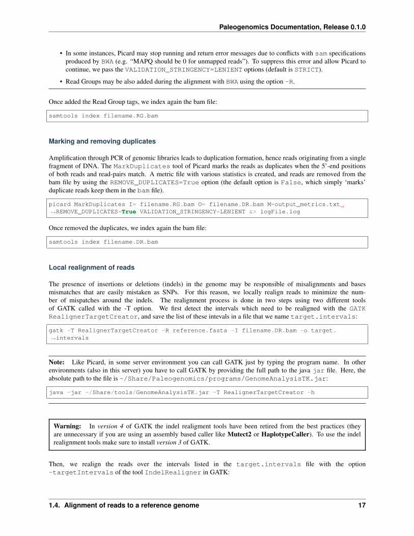
Visualization of reads alignment

Once generated the final bam file, you can compare the bam files before and after the refinement and polishing process(duplicates removal, realignment around indels and sorting). To do so, we will use the program IGV, in which we willfirst load the reference fasta file from Genomes –> Load genome from file and then we will add one (or more) bamfiles with File –> Load from file:

1.4.3 Create mapping summary reports

We will use Qualimap to create summary reports from the generated bam files. As mentioned in the website,Qualimap examines sequencing alignment data in sam/bam files according to the features of the mapped reads andprovides an overall view of the data that helps to detect biases in the sequencing and/or mapping of the data and easesdecision-making for further analysis.

qualimap bamqc -c -bam input.bam

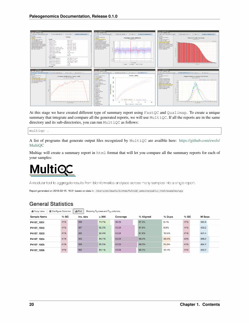
Here are some screenshots of the outputs:

1.4. Alignment of reads to a reference genome 19

Paleogenomics Documentation, Release 0.1.0

At this stage we have created different type of summary report using FastQC and Qualimap. To create a uniquesummary that integrate and compare all the generated reports, we will use MultiQC. If all the reports are in the samedirectory and its sub-directories, you can run MultiQC as follows:

multiqc .

A list of programs that generate output files recognized by MultiQC are availble here: https://github.com/ewels/MultiQC

Multiqc will create a summary report in html format that will let you compare all the summary reports for each ofyour samples:

20 Chapter 1. Contents

Paleogenomics Documentation, Release 0.1.0

1.4.4 Damage analysis and quality rescaling of the BAM file

To authenticate our analysis we will assess the post-mortem damage of the reads aligned to the reference sequence. Wecan track the post-portem damage accumulated by DNA molecules in the form of fragmentation due to depurinationand cytosine deamination, which generates the typical pattern of C->T and G->A variation at the 5’- and 3’-end of theDNA molecules. To assess the post-mortem damage patterns in our bam file we will use mapDamage, which analysesthe size distribution of the reads and the base composition of the genomic regions located up- and downstream of eachread, generating various plots and summary tables. To start the analysis we need the final bam and the referencesequence:

mapDamage -i filename.final.sort.bam -r reference.fasta

mapDamage creates a new folder where the output files are created. One of these files, is namedFragmisincorporation_plot.pdf which contains the following plots:

If DNA damage is detected, we can run mapDamage again using the --rescale-only option and providing thepath to the results folder that has been created by the program (option -d). This command will downscale the qualityscores at positions likely affected by deamination according to their initial quality values, position in reads and damage

1.4. Alignment of reads to a reference genome 21

Paleogenomics Documentation, Release 0.1.0

patterns. A new rescaled bam file is then generated.

mapDamage -i filename.final.sort.bam -r reference.fasta --rescale-only -d results_→˓folder

You can also rescale the bam file directly in the first command with the option --rescale:

mapDamage -i filename.final.sort.bam -r reference.fasta --rescale

Note: Another useful tool for estimating post-mortem damage (PMD) is PMDTools. This program uses a modelincorporating PMD, base quality scores and biological polymorphism to assign a PMD score to the reads. PMD > 0indicates support for the sequence being genuinely ancient. PMDTools filters the damaged reads (based on the selectedscore) in a separate bam file which can be used for downstream analyses (e.g. variant call).

The rescaled bam file has to be indexed, as usual.

samtools index filename.final.sort.rescaled.bam

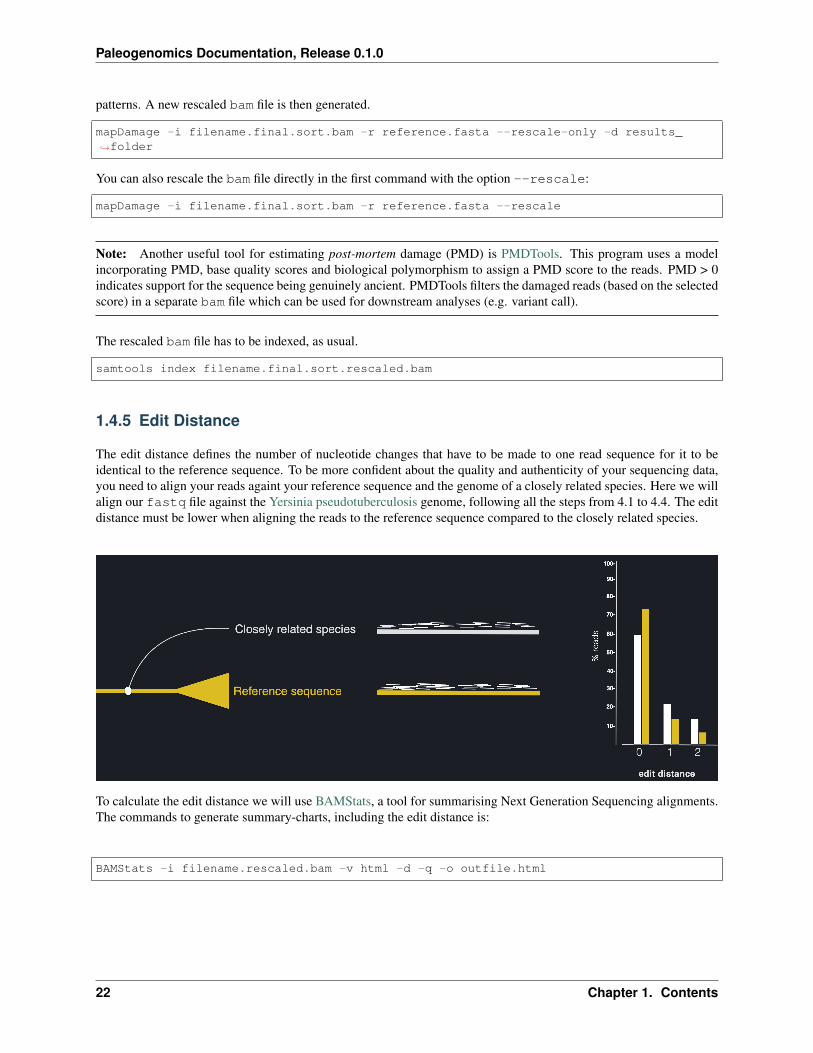
1.4.5 Edit Distance

The edit distance defines the number of nucleotide changes that have to be made to one read sequence for it to beidentical to the reference sequence. To be more confident about the quality and authenticity of your sequencing data,you need to align your reads againt your reference sequence and the genome of a closely related species. Here we willalign our fastq file against the Yersinia pseudotuberculosis genome, following all the steps from 4.1 to 4.4. The editdistance must be lower when aligning the reads to the reference sequence compared to the closely related species.

To calculate the edit distance we will use BAMStats, a tool for summarising Next Generation Sequencing alignments.The commands to generate summary-charts, including the edit distance is:

BAMStats -i filename.rescaled.bam -v html -d -q -o outfile.html

22 Chapter 1. Contents

Paleogenomics Documentation, Release 0.1.0

Option Function-i filename SAM or BAM input file (must be sorted).-vhtml/simple

View option for output format (currently accepts ‘simple’ or ‘html’; default, simple).

-d If selected, edit distance statistics will also be displayed as a separate table (optional).-q If selected, mapping quality (MAPQ) statistics will also be displayed as a separate table (optional).

1.5 Variant calling and visualization

Once the reads are aligned and the data authenticated through post-mortem damage analysis, we can analyse the variantpositions in the samples against the reference sequence.

1.5.1 Variants calling

We will use two common tools for variants calling: Samtools, in particular samtools mpileup, in combinationwith bcftools call of the program BCFtools.

samtools mpileup -B -ugf reference.fasta filename.final.sort.rescaled.bam | bcftools→˓call -vmO z - > filename.vcf.gz

Samtoolsmpileupoptions

Function

-B, –no-BAQ BAQ is the Phred-scaled probability of a read base being misaligned. Applying this option greatlyhelps to reduce false SNPs caused by misalignments.

-u, –uncom-pressed

Generate uncompressed VCF/BCF output, which is preferred for piping.

-g, –BCF Compute genotype likelihoods and output them in the binary call format (BCF). As of v1.0, thisis BCF2 which is incompatible with the BCF1 format produced by previous (0.1.x) versions ofsamtools.

-f, –fasta-reffile

The faidx-indexed reference file in the FASTA format. The file can be optionally compressed bybgzip.

1.5. Variant calling and visualization 23

Paleogenomics Documentation, Release 0.1.0

BCFtoolscall op-tions

Function

-v,–variants-only

Output variant sites only.

-m,–multiallelic-caller

Alternative modelfor multiallelic and rare-variant calling designed to overcome known limitationsin -c calling model (conflicts with -c)

-g, –BCF Compute genotype likelihoods and output them in the binary call format (BCF). As of v1.0, thisis BCF2 which is incompatible with the BCF1 format produced by previous (0.1.x) versions ofsamtools.

-O,–output-type b|u|z|v

Output compressed BCF (b), uncompressed BCF (u), compressed VCF (z), uncompressed VCF (v).

The detected genetic variants will be stored in the vcf file. The genetic variants can be filtered according to somecriteria using BCFtools:

bcftools filter -O z -o filename.filtered.vcf -s LOWQUAL -i'%QUAL>19' filename.vcf.gz

BCFtools filter op-tions

Function

-O, –output-typeb|u|z|v

Output compressed BCF (b), uncompressed BCF (u), compressed VCF (z), uncompressedVCF (v).

-o, –output file Output file.-s, –soft-filterstring|+

Annotate FILTER column with <string> or, with +, a unique filter name generated by theprogram (“Filter%d”).

-i, –include expres-sion

Include only sites for which expression is true.

Note: other options can be added when using BCFtools filter:

Option Function-g, –SnpGap int Filter SNPs within int base pairs of an indel-G, –IndelGapint

Filter clusters of indels separated by int or fewer base pairs allowing only one topass

Instead of samtools mpileup and bcftools call (or in addition to) we can use gatkHaplotypeCaller:

java -jar ~/Share/tools/GenomeAnalysisTK.jar -T HaplotypeCaller -R reference.fasta -I→˓filename.final.sort.rescaled.bam -o filename.vcfjava -jar ~/Share/tools/GenomeAnalysisTK.jar -T VariantFiltration -R reference.fasta -→˓V filename.vcf -o filename.filtered.vcf --filterName 'Qual20|Cov5' --→˓filterExpression 'QUAL<19||DP<5'

Now that you have your vcf file, you can open the file (use nano or vim in the server, or download the file in yourlaptop with scp and open it in a text editor) and try to search diagnostic variants (e.g. for classification). You can also

24 Chapter 1. Contents

Paleogenomics Documentation, Release 0.1.0

visualize the variants in a specific program, as described below.

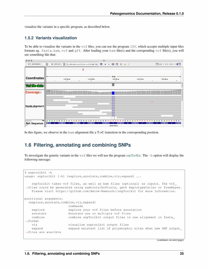
1.5.2 Variants visualization

To be able to visualize the variants in the vcf files, you can use the program IGV, which accepts multiple input filesformats eg. fasta, bam, vcf and gff. After loading your bam file(s) and the corrsponding vcf file(s), you willsee something likt that:

In this figure, we observe in the bam alignment file a T->C transition in the corresponding position.

1.6 Filtering, annotating and combining SNPs

To investigate the genetic variants in the vcf files we will use the program snpToolkit. The -h option will display thefollowing message:

$ snptoolkit -husage: snptoolkit [-h] {explore,annotate,combine,viz,expand} ...

snpToolkit takes vcf files, as well as bam files (optional) as inputs. The vcf→˓files could be generated using samtools/bcftools, gatk HaplotypeCaller or freeBayes.

Please visit https://github.com/Amine-Namouchi/snpToolkit for more information.

positional arguments:{explore,annotate,combine,viz,expand}

commandsexplore explore your vcf files before annotationannotate Annotate one or multiple vcf filescombine combine snpToolkit output files in one alignment in fasta

→˓formatviz visualize snptoolkit output filesexpand expand existent list of polymorphic sites when new SNP output

→˓files are availble

(continues on next page)

1.6. Filtering, annotating and combining SNPs 25

Paleogenomics Documentation, Release 0.1.0

(continued from previous page)

optional arguments:-h, --help show this help message and exit

Five options are possible: explore, annotate, combine, viz, expand.

1.6.1 SNPs filtering and annotion

The snpToolkit annotate command will display general information about the usage of the program:

snptoolkit annotate -husage: snptoolkit annotate [-h] -i IDENTIFIER -g GENBANK [-p PROCESSORS] [-f→˓EXCLUDECLOSESNPS] [-q QUALITY] [-d DEPTH] [-r RATIO] [-e EXCLUDE]

optional arguments:-h, --help show this help message and exit

snpToolkit annotate required options:-i IDENTIFIER provide a specific identifier to recognize the file(s) to be

→˓analyzed-g GENBANK Pleae provide a genbank file

snpToolkit annotate additional options:-p PROCESSORS number of vcf files to be annotated in parallel default value

→˓[1]-f EXCLUDECLOSESNPS exclude SNPs if the distance between them is lower then the

→˓specified window size in bp-q QUALITY quality score to consider as a cutoff for variant calling.

→˓default value [20]-d DEPTH minimum depth caverage. default value [3]-r RATIO minimum ratio that correspond to the number of reads that has

→˓the mutated allele / total depth in that particular position. defaultvalue [0]

-e EXCLUDE provide a tab file with genomic regions to exclude in this→˓format: region start stop. region must correspond to the same name(s) of

chromsome and plasmids as in the genbank file

Here is a simple example on how to use snpToolkit:

snptoolkit annotate -i vcf -g GCF_000009065.1_ASM906v1_genomic.gbff -d 3 -q 20 -r 0.9

snpToolkit can automatically recogninze vcf files generated with the following programs: samtools mpileup,gatk HaplotyCaller and freeBayes. The vcf files could be gzipped or not. In the command line above,snpToolkit will filter and annotate all SNPs in the vcf file(s) that fullfil the following criteria: quality >= 30,depth of coverage >= 5 and ratio >= 0.9.

Note: For each SNP position, the ratio (r) is calculated as follows:

r= dm / (dr + dm)

• dr= Number of reads having the reference allele

• dm= Number of reads having the mutated allele

The output file(s) of snpToolkit is a tabulated file(s) that you can open with Microsoft Excel and it will look as follow:

26 Chapter 1. Contents

Paleogenomics Documentation, Release 0.1.0

##snpToolkit=__version__##commandline= snptoolkit annotate -i vcf -g GCF_000009065.1_ASM906v1_genomic.gbff -d→˓5 -q 30 -r 0.9 -p 4##VcfFile=sample5.vcf.gz##Total number of SNPs before snpToolkit processing: 406##The options -f and -e were not used##Filtred SNPs. Among the 406 SNPs, the number of those with a quality score >= 30, a→˓depth >= 5 and a ratio >= 0.9 is: 218##After mapping, SNPs were located in:##NC_003131.1: Yersinia pestis CO92 plasmid pCD1, complete sequence 70305 bp##NC_003143.1: Yersinia pestis CO92, complete genome 4653728 bp##The mapped and annotated SNPs are distributed as follow:##Location Genes RBS tRNA rRNA ncRNA Pseudogenes intergenic→˓ Synonymous NonSynonumous##SNPs in NC_003143.1: Yersinia pestis CO92, complete genome 4653728 bp 155 0→˓ 0 1 0 0 57 54 101##SNPs in NC_003131.1: Yersinia pestis CO92 plasmid pCD1, complete sequence 70305 bp→˓ 2 0 0 0 0 0 3 1 1##Syn=Synonymous NS=Non-Synonymous##Coordinates REF SNP Depth Nb of reads REF Nb reads SNPs Ratio→˓Quality Annotation Product Orientation Coordinates in gene Ref codon→˓ SNP codon Ref AA SNP AA Coordinates protein Effect Location82 C A 36 0 34 1.0 138.0 intergenic .→˓ + . - - - - - - NC_003143.1:→˓Yersinia pestis CO92, complete genome 4653728 bp130 G C 28 0 27 1.0 144.0 intergenic .→˓ + . - - - - - - NC_003143.1:→˓Yersinia pestis CO92, complete genome 4653728 bp855 G A 69 0 62 1.0 228.0 YPO_RS01010|asnC→˓ transcriptional regulator AsnC - 411 ACC AC[T] T T→˓137 Syn NC_003143.1: Yersinia pestis CO92, complete genome 4653728 bp

The header of the generated snpToolkit output file includes useful information e.g. raw number of SNPs, Number offiltered SNPs, SNPs distribution, etc. . . The SNPs annotation is organized in tab delimited table. The columns of thistable are:

1.6. Filtering, annotating and combining SNPs 27

Paleogenomics Documentation, Release 0.1.0

Column name DescriptionCoordinates SNP coordinateREF Reference alleleSNP New allele in analyzed sampleDepth Total depth of coverageNb of reads REF Number of reads with the reference alleleNb reads SNPs Number of reads with the new alleleRatio Nb reads SNPs/(Nb of reads REF+Nb reads SNPs)Quality Quality scoreAnnotation Distribution within genes or intergenicProduct Functional product of the geneOrientation Gene orientationCoordinates in gene Coordinate of the SNP within the geneRef codon Reference codon, ACC in the example aboveSNP codon New codon, AC[T]Ref AA Amino Acid corresponding to reference codonSNP AA Amino Acid corresponding to new codonCoordinates protein Coordinate of the Amino AcidEffect Could be Synonymous (Syn) or Non-Synonymous (NS)Location ID of the chromosome and plasmids.

1.6.2 Compare and combine multiple annotation files

After generating a set of output files, you can run snpToolkit combine:

$ snptoolkit combine -husage: snptoolkit combine [-h] --location LOCATION [-r RATIO] [--bam BAMFILTER→˓BAMFILTER BAMFILTER] [--snps {ns,s,all,inter}] [-e EXCLUDE]

optional arguments:-h, --help show this help message and exit

snpToolkit combine required options:--location LOCATION provide for example the name of the chromosome or plasmid you

→˓want to create fasta alignemnt for

snpToolkit additional options:-r RATIO new versus reference allele ratio to filter SNPs from

→˓snpToolkit outputs. default [0]--bam BAMFILTER BAMFILTER BAMFILTER

provide the depth, ratio and the path to the folder→˓containing the bam files. eg. 3 0.9 path--snps {ns,s,all,inter}

Specify if you want to concatenate all SNPs or just→˓synonymous (s), non-synonymous (ns) or intergenic (inter) SNPs. default [all]-e EXCLUDE Provide a yaml file with keywords and coordinates to be

→˓excluded

snpToolkit combine will compare all the SNPs identified in each file and create two additional output files:

1) a tabulated files with all polymorphic sites

2) a fasta file.

To combine the snps from different samples in one alignment fasta file you type the following command:

28 Chapter 1. Contents

Paleogenomics Documentation, Release 0.1.0

snptoolkit combine --loc NC_003143.1 -r 0.9 --bam 2 1.0 ../bam

As we will be working with ancient DNA, a small fraction of your genome could be covered. In this case we will usethe option --bam to indicate the path to the folder containing the bam files. The option -d must be used with theoption --bam. By default, all SNPs will be reported. This behaviour can be changed using the option --snp.

Note: It is also possible to use the option --bam with modern data as some genomic regions could be deleted.

The file reporting the polymorphic sites is organized as follows:

ID Coordi-nates

REF SNP Columns with SNP informa-tion

sam-ple1

sam-ple2

sam-ple3

sam-ple4

snp1 130 A T 1 1 1 1snp2 855 C G 0 0 ? 1snp3 1315 A C 1 1 0 0snp4 12086 G A 1 0 ? 0

The table above reports the distribution of all polymorphic sites in all provided files. As we provided the bam filesof the ancient DNA samples, snpToolkit will check if the polymorphic sites (snp2 and snp4) are absent in sample3because there is no SNP in that positions or because the region where the snps are located is not covered. In the lattercase, snpToolkit will add a question mark ? that reflects a missing data. From the table above, it will be possible togenerate a fasta file, like the one below:

>ReferenceATCGGGTATGCCAATGCGT>Sample1ACCGGGTATGCCAATGTGT>Sample2ATTGGGTATGCCAGTGCGT>Sample3?TTGAGT?TGTCA?TACGT>Sample4ATCGGGTATGCCAATGCGT

The fasta output file will be used to generate a maximum likelihood tree using IQ-TREE

1.6.3 Phylogenetic tree reconstruction

There are several tools to build phylogenetic trees. All of these tools, use an alignment file as input file. Now that wehave generated an alignment file in fasta format, we will use IQ-TREE to build a maximum likelihood tree. Weuse IQ-TREE for several reasons:

• It performs a composition chi-square test for every sequence in the alignment. A sequence is denoted failed ifits character composition significantly deviates from the average composition of the alignment.

• Availability of a wide variety of phylogenetic models. IQ-TREE uses ModelFinder to find the best substitutionmodel that will be used directly to build the maximum likelihood phylogenetic tree.

• Multithreading

To generate the phylogenetic tree type the following command using your fasta as input:

iqtree -m MFP+ASC -s SNPs_alignment.fasta

1.6. Filtering, annotating and combining SNPs 29

Paleogenomics Documentation, Release 0.1.0

IQ-TREE options Function-m Substitution model name to use during the analysis.-s Alignment file

More information of IQ-TREE can be found in the program’s tutorial

The phylogenetic tree generated can be visualized using Figtree, download it in your local machine and load thetreefile output from IQ-TREE to visualize the tree.

1.7 DO-IT-YOURSELF

1.7.1 Hands-on 1: ancient human mtDNA

In this final hands-on session you will analyse shotgun (reduced) sequencing data generated from an ancient humantooth.The genomic library built from the DNA extract was sequenced on an Illumina platform in paired-end mode.Your task is:

1. Process the raw reads (remove adapters, merge the reads, section 2).

2. Align the reads to the human mitochondrial DNA (mtDNA) reference sequence, assess the damage of DNAmolecules, call the variants (sections 4-5-6).

3. Run the metagenomic screning of the DNA extract with Kraken using the Minikraken database (section 3).

After reads pre-processing it is up to you whether first aliging the reads or screening the metagenomic content.

• Option 1: You can use your vcf file to assign an haplogroup to the human samples that you analysed. Someuseful tools for haplogroup assignation:

– Check the variant positions in Phylotree (http://www.phylotree.org/)

– Load the vcf file in Haplogrep (https://haplogrep.uibk.ac.at)

• Option 2: Run again the metagenomic screening with a Custom Database of Kraken (provided by us), andcompare the results with those obtained with Minikraken.

1.7.2 Hands-on 2: ancient human dental calculus

In this hands-on you will use a sequence dataset of ancient dental calculus from a recent study by Velsko et al.(Microbiome, 2019), which consists of paired-end sequence data. After filtering and collapsing the reads, classify thereads of each sample with Kraken2 and estimate the abudances with Bracken.

After that, you can use R to run analyses and create charts from the abundance tables generated with Bracken. Runthe following R script to merge the species aundances of all the samples in one table. The script needs as argument thepath to the folder containing the bracken results. Move to the bracken results folder and type the following command:

Rscript brackenToAbundanceTable.R .

The script will generate two abundance tables, taxa_abundance_bracken_IDs.txt, which contains thespecies names as NCBI IDs, and taxa_abundance_bracken_names.txt, which contains the actual speciesnames. Since the Minikraken database was built from complete Bacterial, Archaeal and Viral genomes, we must

30 Chapter 1. Contents

Paleogenomics Documentation, Release 0.1.0

make a normalization for the genome leghts of each species. This normalization is important when we want to anal-yse relative taxa abundances to characterise full microbiomes. To do that will use a Python script that takes threearguments:

1) The abundance table

2) The table of genome legths

3) The name of the output file

To run the normalization type the command:

python gL-normalizer-lite.py taxa_abundance_bracken_names.txt prokaryotes_viruses_→˓organelles.table taxa_abundance_bracken_names_normalized.txt

R session

Now can download the normalized table in your local machine (e.g. with scp) and open R.

First of all, in R, we must set up the folder which contains the abundance table:

setwd("/path/to/your/folder")

Then we can import the abundance table files, setting the 1st column as row names. Then we remove the 1st, 2nd and3rd column, which will not be used for the analysis.

table.species = read.delim("taxa_abundance_bracken_names_normalized.txt", header=T,→˓fill=T, row.names=1, sep="\t")table.species.final = table.species[,-c(1:3)]

Then we filter the species in the table for their abundance by removing those that are represented below a threshold of0.02%. First we define a function (that we call low.count.removal)

low.count.removal = function(data, # OTU count data frame of size n

→˓(sample) x p (OTU)percent=0.02 # cutoff chosen){

keep.otu = which(colSums(data)*100/(sum(colSums(data))) > percent)data.filter = data[,keep.otu]return(list(data.filter = data.filter, keep.otu = keep.otu))

}

We run the function on our table, setting up the threshold at 0.02%:

result.filter = low.count.removal(t(table.species.final), percent=0.02)

We generate a table with the filtered data:

table.species.final.flt = result.filter$data.filter

In the next step, we normalize the reads for the sequencing depth. This means that we will account for the total readsgenerated for each sample, and normalize the species abundance for that number. To do that we will define a TotalSum Squared function

TSS.divide = function(x){x/sum(x)

}

1.7. DO-IT-YOURSELF 31

Paleogenomics Documentation, Release 0.1.0

The function is applied to the table, and each row must represent a sample. For this reason we transpose the table.

table.species.final.flt.tss = t(apply(table.species.final.flt, 1, TSS.divide))

We have just generated a table of species abundances of ancient dental calculus samples, normalized for genomelenghts and sequencing depths. We can now include in our analysis a dataset of normalized species abundancesgenerated with Kraken2 representing other microbiomes. You can find this table in the server, download it and importit in R.

microbiomes.literature = read.table("microbiomes_literature.txt", header=T, fill=T,→˓row.names=1, sep="\t")

The following commands are used to merge the two tables, the dental calculus dataset that you generated and the othermicrobiomes dataset.

table.total = merge(t(table.species.final.flt.tss), t(microbiomes.literature), by=0,→˓all=TRUE)table.total[is.na(table.total)] <- 0row.names(table.total) = table.total[,1]table.total.final = t(table.total[,-1])

UPGMA

Once generated the final including both datasets (dental calculus and other microbiomes), we run an UPGMA clusteranalysis. We must first install the vegan and ape package in R.

install.packages("vegan")install.packages("ape")library(vegan)library(ape)

Then we use vegan to calculate the Bray-Curtis distances, and run the cluster analysis.

bray_dist = vegdist(table.total.final, method = "bray", binary = FALSE, diag = FALSE,→˓upper = FALSE, na.rm = FALSE)bray_dist.clust = hclust(bray_dist, method="average", members = NULL)

Finally, we plot the dendrogram:

plot(as.phylo(bray_dist.clust), type = "unrooted", cex = 0.5, lab4ut="axial", no.→˓margin=T, show.tip.label=T, label.offset=0.02, edge.color = "gray", edge.width = 1,→˓edge.lty = 1)

To visualize better our samples, we can define colors. We will assign group labels on each sample:

labels = c("Velsko-ancient","Velsko-ancient","Velsko-ancient","Velsko-ancient",→˓"Velsko-ancient","Velsko-ancient","Velsko-ancient","Velsko-ancient","Velsko-ancient→˓","Velsko-ancient",

"Velsko-modern","Velsko-modern","Velsko-→˓modern","Velsko-modern","Velsko-modern","Velsko-modern","Velsko-modern","Velsko-→˓modern",

"Ancient calculus","Ancient tooth",→˓"Ancient calculus","Ancient tooth",

"Soil","Soil","Soil","Soil","Soil","Soil→˓","Soil",

"Ancient calculus","Ancient tooth",→˓"Ancient calculus","Ancient tooth","Ancient calculus","Ancient tooth","Ancient→˓calculus","Ancient tooth","Ancient calculus","Ancient tooth","Ancient calculus",→˓"Ancient tooth",

(continues on next page)

32 Chapter 1. Contents

Paleogenomics Documentation, Release 0.1.0

(continued from previous page)

"Plaque","Plaque","Plaque","Plaque",→˓"Plaque","Plaque","Plaque","Plaque","Plaque","Plaque",

"Plaque","Plaque","Plaque","Plaque",→˓"Plaque","Plaque","Plaque","Plaque","Plaque","Plaque",

"Plaque","Plaque","Plaque","Plaque",→˓"Plaque",

"Skin","Skin","Skin","Skin","Gut","Gut","Gut","Gut","Gut","Gut","Gut

→˓","Gut","Gut","Gut","Gut","Gut","Gut","Gut","Gut","Gut","Gut

→˓","Gut","Gut","Gut","Gut","Gut","Gut","Gut","Skin","Skin","Skin","Skin","Skin","Plaque","Plaque")

To have a better look at the correspondence of data we can create a dataframe:

table.total.final.df = as.data.frame(table.total.final)table.total.final.df$group = labels

We assign colors to each label:

coul=c("#E41A1C", #Ancient calculus"#419681", #Ancient tooth"#4DAF4A", #Gut"lightgray", #Plaque"#984EA3", #Skin"#FF7F00", #Soil"goldenrod", #Velsko-ancient"#994C00") #Velsko-modern

And finally, we plot again the dendrogram, this time by customizing the tips assigning color-coded labels:

plot(as.phylo(bray_dist.clust), type = "unrooted", cex = 0.5, lab4ut="axial", no.→˓margin=T, show.tip.label=T, label.offset=0.02, edge.color = "gray", edge.width = 1,→˓edge.lty = 1)tiplabels(pch=19, col = coul[factor(labels)], bg = coul[factor(labels)], cex=1, lwd=1)

And we can add a legend:

legend("topleft", legend = sort(unique(labels)), bty = "n", col = coul, pch = 19, pt.→˓cex=1, cex=0.6, pt.lwd=1)

1.8 Material from previous courses

1.8.1 Kraken

In this hands-on session we will use Kraken to screen the metagenomic content of a DNA extract after shotgunsequencing. A Kraken database is a directory containing at least 4 files:

• database.kdb: Contains the k-mer to taxon mappings

• database.idx: Contains minimizer offset locations in database.kdb

• taxonomy/nodes.dmp: Taxonomy tree structure + ranks

1.8. Material from previous courses 33

Paleogenomics Documentation, Release 0.1.0

• taxonomy/names.dmp: Taxonomy names

Minikraken

We will first use a pre-built 8 GB Kraken database, called Minikraken, constructed from complete dusted bacterial,archaeal, and viral genomes in RefSeq (as of October 2017). You can download the pre-built Minikraken databasefrom the website with wget, and extract the archive content with tar:

wget https://ccb.jhu.edu/software/kraken/dl/minikraken_20171101_8GB_dustmasked.tgztar -xvzf minikraken_20171101_8GB_dustmasked.tgz

Then, we can run the taxonomic assignation of the reads in our sample with the kraken command

kraken --db minikraken_20171101_8GB_dustmasked --fastq-input filename.gz --gzip-→˓compressed --output filename.kraken

Some of the options available in Kraken:

Option Function–db <string> Path to the folder (database name) containing the database files.–output <string> Print output to filename.–threads <integer> Number of threads (only when multiple cores are used).–fasta-input Input is FASTA format.–fastq-input Input is FASTQ format.–gzip-compressed Input is gzip compressed.

Create report files

In Kraken 1, report files are generated with a specific command, after the classification (section 3.1.2: Create reportfiles). Once the taxonomic assignation is done, from the Kraken output file we create a report of the analysis byrunning the kraken-report script. Note that the database used must be the same as the one used to generate theoutput file in the command above. The output file is a tab-delimited file with the following fields, from left to right:

1. Percentage of reads covered by the clade rooted at this taxon

2. Number of reads covered by the clade rooted at this taxon

3. Number of reads assigned directly to this taxon

4. A rank code, indicating (U)nclassified, (D)omain, (K)ingdom, (P)hylum, (C)lass, (O)rder, (F)amily, (G)enus, or(S)pecies. All other ranks are simply ‘-‘.

5. NCBI taxonomy ID

6. Indented scientific name

Notice that we will have to redirect the output to a file with >.

kraken-report --db Minikraken filename.kraken > filename.kraken.report

Note: We can use a for loop to make the taxonomic assignation and create the report file for multiple samples.Notice the assignation of variables filename and fname to return output files named after the sample.

34 Chapter 1. Contents

Paleogenomics Documentation, Release 0.1.0

for i in *.fastqdo

filename=$(basename "$i")fname="${filename%.fastq}"kraken --db Minikraken --threads 4 --fastq-input $i --output /${fname}.krakenkraken-report --db Minikraken ${fname}.kraken > ${fname}.kraken.report

done

To visualize the results of the classification in multi-layerd pie charts, use Krona, as described in the section 3.1.2(see Visualization of data with Krona).

Building a Kraken standard database (on HPC clusters)

The pre-built Minikraken database is useful for a quick metagenomic screening of shotgun data. However, by buildinglarger databases (i.e. a larger set of k-mers gathered) we may increase the sensitivity of the analysis. One option is tobuild the Kraken standard database. To create this database we use the command kraken-build, which downladsthe RefSeq complete genomes for the bacterial, archaeal, and viral domains, and builds the database.

kraken-build --standard --db standardkraken.folder

Note:

• Usage of the database will require users to keep only the database.idx, database.kdb, taxonomy/nodes.dmp and taxonomy/names.dmp files. During the database building process some intermediate fileare created that may be removed afterwards with the command:

kraken-build --db standardkraken.folder --clean

• The downloaded RefSeq genomes require 33GB of disk space. The build process will then require approxi-mately 450GB of additional disk space. The final database.idx, database.kdb, and taxonomy/ filesrequire 200 Gb of disk space, and running one sample against such database requires 175 Gb of RAM.

Building a Kraken custom database (on HPC clusters)

Building kraken custum databases is computationally intensive. You will find a ready to use database. Kraken alsoallows creation of customized databases, where we can choose which sequences to include and the final size of thedatabase. For example if you do not have the computational resources to build and run analyses with a full databaseof bacterial genomes (or you don’t need to), you may want to build a custom database with only the genomes neededfor your application.

1. First of all we choose a name for our database and we create a folder with that name using mkdir. Let’s callthe database CustomDB. This will be the name used in all the dollowing commands after the --db option.

2. Download NCBI taxonomy files (the sequence ID to taxon map, the taxonomic names and tree information)with kraken-build --download-taxonomy. The taxonomy files are necessary to associate a taxon tothe sequence identifier (the GI number in NCBI) of the fasta sequences composing our database. For thisreason we will build our database only with sequences from the NCBI RefSeq. For more information on theNCBI taxonomy visit click here. This command will create a sub-folder taxonomy/ inside our CustomDBfolder:

1.8. Material from previous courses 35

Paleogenomics Documentation, Release 0.1.0

kraken-build --download-taxonomy --threads 4 --db CustomDB

3. Install a genomic library. RefSeq genomes in fasta file from five standard groups are made easily available inKraken with the command kraken-build –download-library:

• bacteria : RefSeq complete bacterial genomes

• archaea : RefSeq complete archaeal genomes

• plasmid : RefSeq plasmid sequences

• viral : RefSeq complete viral genomes

• human : GRCh38 human genome

The following command will download all the RefSeq bacterial genomes (33Gb size) and create a folderlibrary/ with a sub-folder bacteria/ inside your CustomDB folder:

kraken-build --download-library bacteria --threads 4 --db CustomDB

4. We can add any sort of RefSeq fasta sequences to the library with kraken-build --add-to-library.For example we will add to the library of bacterial genomes the RefSeq sequences of mitochodrial genomes.The sequences will be inside the sub-folder added/.

kraken-build --add-to-library mitochondrion.1.1.genomic.fna --threads 4 --db→˓CustomDBkraken-build --add-to-library mitochondrion.2.1.genomic.fna --threads 4 --db→˓CustomDB

Note: If you have several fasta files to add you can use a for loop:

for i in *.fastadokraken-build --add-to-library $i --threads 4 --db CustomDB

done

5. When analyzing a metagenomics sample using a Kraken database the primary source of false positive hits isrepresented by low-complexity sequences in the genomes themselves (e.g., a string of 31 or more consecutiveA’s). For this reason, once gathered all the genomes that we want to use for our custom database, low-complexityregions have to be ‘dusted’. The program dustmasker from Blast+ identifies low-complexity regions andsoft-mask them (the corresponding sequence is turned to lower-case letters). With a for loop we run dust-masker on each fasta file present in the library folder, and we will pipe (|) to dustmasker a sed command toreplace the low-complexity regions (lower-case) with Ns. Notice that the output is redirected (>) to a temporaryfile, which is afterwards renamed to replace the original file fasta file with the command mv.

for i in `find CustomDB/library \( -name '*.fna' -o -name '*.ffn' \)`dodustmasker -in $i -infmt fasta -outfmt fasta | sed -e '/>/!s/a\|c\|g\|t/N/g' >

→˓tempfilemv -f tempfile $i

done

Some of the options available in Dustmasker:

36 Chapter 1. Contents

Paleogenomics Documentation, Release 0.1.0

Option Function-in <string> input file name-infmt <string> input format (e.g. fasta)-outfmt8 <string> output format (fasta)

6. Finally, we build the database with kraken-build. With this command, Kraken uses all the masked genomescontained in the library (bacteria and mtDNA RefSeq) to create a database of 31 bp-long k-mers. We canchoose the size of our custom database (hence the number of k-mers included, and the sensitivity) with the--max-db-size option (8 Gb here).

kraken-build --build --max-db-size 8 --db CustomDB

Taxonomic assignation with Kraken custom database

Once our custom database is built we can run the command for taxonomic assignation of DNA reads agaisnt thecustom database, as in section 1.1 and 1.2.

kraken --db CustomDB --fastq-input merged.fastq.gz --gzip-compressed --output sample.→˓krakenkraken-report --db CustomDB sample.kraken > sample.kraken.report

Or, again, we can loop the commands if we have various samples.

for i in *.fastqdo

filename=$(basename "$i")fname="${filename%.fastq}"kraken --db CustomDB --threads 4 --fastq-input $i --output ${fname}.krakenkraken-report --db CustomDB ${fname}.kraken > ${fname}.kraken.report

done

To visualize the results of the classification in multi-layerd pie charts, use Krona, as described in the section 3.1.3:Visualization of data with Krona

Course overview

1.8. Material from previous courses 37

Paleogenomics Documentation, Release 0.1.0

• genindex

• modindex

• search

38 Chapter 1. Contents