Chapter 2

Paleoclimatic Ocean Circulationand Sea-Level Changes

Stefan Rahmstorf and Georg FeulnerPotsdam Institute for Climate Impact Research, Potsdam, Germany

Chapter Outline1. Introduction 31

2. Reconstructing Past Ocean States 32

2.1. Proxies for Past Ocean Circulation 32

2.1.1. Nutrient Water Mass Tracers 32

2.1.2. Conservative Water Mass Tracers 33

2.1.3. Circulation Rate Tracers 34

2.1.4. Other Tracers 34

2.2. Past Sea-Level Proxies 34

2.2.1. Coastal Morphology and Corals 35

2.2.2. Sediment Cores 36

2.2.3. Manmade Sea-Level Indicators 37

2.3. Models 38

3. The Oceans in the Quaternary 39

3.1. The Last Glacial Maximum 40

3.2. Abrupt Glacial Climate Changes 42

3.2.1. Deglaciation 44

3.3. Glacial Cycles 45

3.4. Interglacial Climates 46

4. The Deeper Past 46

4.1. Challenges of Deep-Time Paleoceanography 46

4.2. The Oceans During the Mid-Cretaceous Warm Period 48

5. Outlook 51

Acknowledgments 52

References 52

1. INTRODUCTION

The oceans have been an important factor in shapingEarth’s past climate. Their circulation has influenced theoverlying atmosphere (see, e.g., reviews of Alley et al.,2002; Clark et al., 2002; Rahmstorf, 2002) and they haveacted, as they still do, as a repository for heat and gases.One consequence of the ocean’s response to climatechange, which is acutely important for human society, issea-level change (the book Understanding sea-level riseand variability edited by Church et al., 2010 gives anexcellent overview of this topic; see Chapter 27). Thischapter provides a brief introductory discussion of pastocean circulation and sea-level changes before the timeof instrumental measurements.

We describe the methods used for reconstructing pastocean states using proxy data and models and give specificexamples of ocean circulation and sea-level changes inEarth’s history. This is a large field with a vast body of sci-entific literature, thanks to a great research community withmany excellent scholars, and this chapter can certainly not

provide a comprehensive review. Rather, we provide thereader with an introduction to some of the main methods,together with examples of the research questions beingaddressed. Inevitably, the choice of examples is to someextent subjective and dependent on the authors’ areas ofexpertise. However, we hope to provide a basis of under-standing this exciting and important topic in which manypuzzles still wait to be solved.

The dominant drivers of paleoclimatic change dependon the timescale considered. Two important ones are tec-tonic and orbital timescales (Ruddiman, 2000). The formercovers climatic changes on timescales of some millions ofyears up to the age of the Earth of 4.6 billion years. Thesechanges are driven by tectonic processes associated with thesolid Earth’s internal heat, but also include the evolution oflife which has altered the composition of Earth’s atmo-sphere (Stanley, 2005). Plate tectonics are a key driver ofEarth’s long-term carbon cycle which controls atmosphericCO2 concentration on multimillion year timescales byexchanging carbon with the Earth’s crust. Plate tectonicsalso alter the Earth’s geography with effects on climate, that

Ocean Circulation and Climate, Vol. 103. http://dx.doi.org/10.1016/B978-0-12-391851-2.00002-7Copyright © 2013 Elsevier Ltd. All rights reserved. 31

is, the position of continents and oceans, the formation ofmountain ranges, and the opening or closing of oceangateways.

On timescales of thousands to hundreds of thousands ofyears, the Earth’s orbital cycles are an important (probablydominant) driver of climate changes. These Milankovitchcycles (Milankovitch, 1941) have main periods of23,000 years (precession), 41,000 years (tilt of Earth’saxis), and !100,000 as well as !400,000 years (eccen-tricity of Earth’s orbit) and have a strong effect on the sea-sonal and latitudinal distribution of solar radiation(Ruddiman, 2000). These orbital cycles are pacemakersof the Quaternary glaciations (see Section 3).

In addition, climate has been changed by variability inthe sun’s radiation output and by internal processes in theclimate system, such as through instabilities in ocean circu-lation or ice sheets. It is important to distinguish betweenchanges in global-mean temperature (primarily dependenton Earth’s global radiation balance but with small transientvariations due to changes in ocean heat storage; Chapter 27)and those climate changes caused by redistribution of heatsuch as through changing oceanic or atmospheric heattransport (Chapter 29).

2. RECONSTRUCTING PAST OCEANSTATES

Past changes in ocean circulation and sea level have left anumber of lasting records that can still be sampled today,for example, in the form of sediments on the ocean floor,uplifted marine terraces, or ancient corals. In order tointerpret these proxy data and to provide quantitatively con-sistent scenarios of past ocean states and changes, a range ofmodels is used. The combination of proxy data and modelsallows us to formulate and test hypotheses about mecha-nisms of past ocean and climate changes.

2.1. Proxies for Past Ocean Circulation

Although there are numerous sources of information aboutpast ocean states in the sedimentary record, it is not easy tointerpret this information in terms of specific changes inocean circulation. In fact, this is an inverse problem wherethe products of a given ocean circulation (in terms of sed-iment deposition) are used to infer what the ocean circu-lation state may have been. Solving this inverse problemis complicated by the fact that what is found in the sedi-mentary record is usually the result of multiple influencingfactors, the data have uncertainties both in dating and in theparameter values measured, and their time resolution isoften seriously limited (e.g., by bioturbation of the sed-iment) so that they need to be interpreted as some kind oftime average.

Tracers of past ocean circulation can be broadly groupedinto three types: nutrient-type water mass tracers, conser-vative water mass tracers, and circulation rate tracers. Inaddition, special cases are the neodymium isotope ratiosand nongeochemical tracers. An excellent, much moredetailed review along these lines is found in Lynch-Stieglitz (2003); see also Chapter 26.

2.1.1. Nutrient Water Mass Tracers

Nutrient water mass tracers are those elements that areinvolved in biological activity and thus behave likenutrients, that is, like the key constituents of marine organicmatter: carbon, nitrogen, and phosphorus. These are takenup by marine life during primary production near the oceansurface and hence tend to be depleted in surface waters. Inmany parts of the ocean, nitrogen or phosphorus are close tozero concentration at the surface since their availability isthe limiting factor of primary production (these are bio-limiting elements). As dead organic matter sinks throughthe water column and decays there or on the seafloor,nutrients are returned to the water. Thus, water masses typ-ically gain in nutrient concentration over time after theyhave left the surface ocean. In the present-day Atlantic,the main water masses of Antarctic Intermediate Water(AAIW), North Atlantic Deep Water (NADW), andAntarctic BottomWater (AABW) reflect the initial nutrientcontent set by the respective surface value in the water massformation region and by subsequent mixing between thesewater masses. In the deep Pacific Ocean, nutrient contentreflects the initial value of the inflowing AABW, progres-sively increasing as the water mass ages along the pathwaythat it spreads.

The basic principle behind the use of nutrient-stylewatermass tracers is to use elements (or isotopes of ele-ments) that behave like nutrients but that are preserved insediments (typically in the calcium carbonate shells ofbottom dwelling marine organisms such as foraminifera),so that their distribution during past epochs can be mappedusing a large number of sediment cores from different oceandepths. Prominent among these tracers are carbon isotoperatios (d13C) (Deuser and Hunt, 1969) and the cadmium/calcium ratio (Cd/Ca) (Boyle et al., 1976).

A basic precondition for using the composition of shells(or “tests”) of marine organisms as water mass indicators isthat the chemical composition of these shells faithfullyreflects that of the seawater they grew in. This is illustratedfor two species of foraminifera in Figure 2.1 for their carbonisotope ratios.

The choice of species is important: not all are as wellsuited as the two shown. Biological processes can lead topreferential uptake of the lighter 12C as compared to 13C,so that a systematic offset arises between d13C (a measureof relative 13C content) in the shells relative to the ambient

PART I The Ocean’s Role in the Climate System32

water (Wefer and Berger, 1991). This is generally the casefor planktonic foraminifera (i.e., those living in the watercolumn), which thus do not record water mass propertiesas well as the benthic (i.e., bottom dwelling) species shownin Figure 2.1 (Spero and Lea, 1996). Hence, benthic forami-nifera are commonly used to reconstruct past deepwatermasses. Within benthic foraminifera, differences betweenspecies are thought to mainly arise because of their differentchoices of microhabitat (e.g., Tachikawa and Elderfield,2002). Some (e.g., Uvigerina) live not on the surface ofthe sediments but within the pore water, which is depletedin d13C relative to the bottom water. This example high-lights that much experience and a detailed understandingof the processes is required in order to arrive at robust con-clusions from proxy data; it takes considerable time anddetective work to develop proxies to the level where theycan be properly interpreted.

The Cd/Ca ratio in shells of benthic foraminifera isanother commonly used proxy for nutrient cycling in theocean, because these elements are incorporated in the shellsin proportion to their abundance in the water. However,there is a depth-dependent empirical factor that needs tobe accounted for in reconstructing seawater cadmium con-centrations from the shells (Boyle, 1992).

Cadmium in seawater is distributed much like majornutrients (e.g., phosphorus)—indeed it shows an almostlinear relationship to phosphorus. Apparently, marineplankton metabolize cadmium like a nutrient, so it isdepleted in warm surface waters where primary produc-tivity occurs and enriched in deepwaters where organicmatter decays (Boyle et al., 1976). A complication that

needs to be considered in the interpretation is that the bio-logical relation between cadmium and phosphorus is notexactly linear due to preferential uptake, so that a curvedP versus Cd relation is expected along a water mass thatis progressively nutrient-depleted by biological activity(Elderfield and Rickaby, 2000). In contrast, a straightmixing line would be obtained by progressive mixing oftwo distinct water masses with low and high nutrientcontent.

Further nutrient-style tracers include barium and zinc,measured as Ba/Ca and Zn/Ca ratios, respectively(Lynch-Stieglitz, 2003).

2.1.2. Conservative Water Mass Tracers

Conservative water mass tracers are those that (in contrastto nutrients) have no sources or sinks in the subsurfaceocean, so that their properties are set at the ocean surfaceand the variations deeper in the water column reflect thetransport and mixing of water masses (see Chapters 6–8and 26). This is the case with temperature and salinity,the standard water mass tracers of modern physical ocean-ography. Such a conservative tracer is magnesium, as theMg/Ca ratio in benthic foraminifera reflects the water tem-perature during calcification, that is, that in which theorganisms lived (Rosenthal et al., 1997). The major chal-lenge here is to determine the water temperature fromMg/Ca with sufficient accuracy in order to reconstructthe relatively small gradients in deepwater temperatures.

Another common conservative tracer is the oxygenisotope ratio, expressed as d18O (i.e., the relative deviationof 18O content from a standard). The d18O value of oceanwater is set at the surface depending on water exchange(e.g., by evaporation and precipitation), hence it is closelylinked to salinity (Lynch-Stieglitz, 2003). Since 18O isheavier than the common 16O, it evaporates less easily.Therefore, continental ice (made from snow) is depletedin 18O and the formation of large ice sheets leads to asizeable increase in 18O in ocean water. During the lastglacial maximum (LGM), sea level was!130 m lower thantoday; the missing water was 18O depleted and stored onland in the form of ice. The remaining water thereforewas proportionally 18O enriched by about 1% in d18O. Infact, this glacial 18O peak can still be found today in the porewater of sediments formed at the time, now typically foundat a depth of 20–60 m within the sediments, depending onlocation (Schrag et al., 2002).

The d18O in the calcite shells of foraminifera depends onthat of the surrounding waters and on the temperature (thereis a temperature-dependent biological fractionation) (e.g.,Duplessy et al., 2002). Hence, if the d18O of the water orthe salinity and ice volume effect is known (or negligible),d18O in these shells can be used as a proxy for local temper-ature (Figure 2.2). The slope shown there suggests that

Estimated seawater d13C (‰ PDB)

d13 C

rec

onst

ruct

ed fr

om fo

ram

inife

ra (

‰ P

DB

)

!0.40!0.40

0.00

0.40

0.80

1.20

1.60

0.00 0.40 0.80 1.20 1.60

FIGURE2.1 Carbon isotopic composition of core top benthic foraminifera

in the genera Cibicidoides and Planulina versus estimated carbon isotopic

composition of dissolved inorganic carbon in the water column above core

location. From Lynch-Stieglitz (2003) after Duplessy et al. (1984).

Chapter 2 Paleoclimatic Ocean Circulation and Sea-Level Changes 33

benthic d18O in calcite increases by !0.25% per "C.However, d18O is useful as a water mass tracer even ifthe effects of temperature and salinity cannot be separated,since they are both conservative tracers (Lynch-Stieglitz,2003).

2.1.3. Circulation Rate Tracers

The tracers discussed so far provide information on thewater masses present in the past at locations for whichwe have sediment data, including on the relative contri-bution of waters from different source regions and thus rel-ative renewal rates. But they do not reveal the rates ofocean circulation. Various methods have been applied toestimate rates.

One set of techniques uses radiocarbon (14C), which iscreated in the atmosphere due to cosmic rays. While thesurface ocean is close to equilibrium with atmosphericradiocarbon content, this decays below the surfaceaccording to the half-life of 14C of 5730 years. In themodern ocean, this is a very useful measure of the age ofwater masses, that is, the time elapsed since they left thesurface (Stuiver et al., 1983).

The problem with using 14C in paleoclimatic studies isthat it continues to decay after it is incorporated in calciteshells, so that the time recorded by 14C ages of benthic fora-minifera is the age of the deepwater plus the age of the fora-minifera shell. To derive the deepwater age, an independentmeasure of the shell age is needed. This can be derived fromthe age of planktonic foraminifera collocated in the samesediment (Broecker et al., 1988). Or the method is appliedto benthic corals, which can be dated independently usinguranium dating (Adkins et al., 1998).

Another approach is measuring the ratio of protactiniumto thorium, 231Pa/230Th. These elements are created uni-formly throughout the water column by uranium decay

and rapidly removed into the sediments by reacting withsinking marine particles (Anderson et al., 1983). Sincethe efficiency with which both elements are removed is dif-ferent, their ratio depends on how long this removal processhas operated, for example, along the path of NADWflowing south in the Atlantic. This method has been usedto infer NADW flow rates during the LGM (Yu et al.,1996). However, this ratio is also sensitive to particle fluxesand composition and interpretation is not straightforward.

Finally, the geostrophic method, a standard approach inphysical oceanography, can also be applied to paleoclimate.It requires knowledge of density profiles in the past upperocean, which can be estimated from d18O in benthic forami-nifera (see Section 2.1.2). This method has been used toreconstruct past Gulf Stream flow in the Florida Straits(Lynch-Stieglitz et al., 1999). To reconstruct density pro-files, benthic foraminifera are required from different depthlevels and thus a range of cores from different water depths.

2.1.4. Other Tracers

Some other tracers exist, that neither behave like nutrients(i.e., with biological sources and sinks) nor are conser-vative. An example is neodymium isotopes, which havesources and sinks at the ocean–sediment interface, becauseneodymium precipitates in metallic crusts or is mobilizedfrom detrital material. This gives water masses like NADWa distinctive neodymium isotope signature that can be usedto assess the mixing of water masses of different origin(Rutberg et al., 2000).

2.2. Past Sea-Level Proxies

When studying sea level, we first need to distinguish rel-ative from absolute sea-level changes. Absolute sea-levelchanges are changes in the sea surface height with respect

!3

!2

!1

0

1

2

3

4

0 5 10 15 20 25 30

"18 O

calc

ite (

PD

B)

- d1

8 Ow

ater

(P

DB

)

Temperature (°C)

Lynch-Stieglitz et al. (1999)Duplessy et al (2002)Kim and O’Neil (1997)

FIGURE 2.2 The isotopic fractionation, expressed asthe difference between the d18O of foraminiferal

calcite and the d18O of seawater versus temperature

of calcification. Cibicidoides and Planulina fromLynch-Stieglitz et al. (1999) (—#) and Duplessy

et al. (2002) (—$) are shown along with the inorganicprecipitation experiments of Kim and O’Neil (1997)

(D). From Lynch-Stieglitz (2003).

PART I The Ocean’s Role in the Climate System34

to a fixed absolute reference frame, for example, the centerof the Earth, as measured from a satellite. Relative sea-levelchange is what an observer (or tide gauge) at the coastwould have experienced. It is measured locally, relativeto the land and is thus the sum of absolute sea-level changesand vertical motions of the land. In the recent geologicalpast (last !4000 years), vertical land motion was the dom-inant factor of relative sea-level change on many coastlines.

Within absolute sea-level changes, it is useful to distin-guish local from global changes. There are mechanisms(e.g., a change in wind regime) that can change sea levellocally without having any effect on global-mean watervolume and sea level. Changes in global-mean (or eustatic)sea level consist of changes in the volume of seawater(arising either from mean density changes or from additionof water, e.g., from melting continental ice) and of changesin the volume of the ocean basins that contain it (due to platetectonics or isostatic adjustment).

Past sea-level changes are reconstructed using sea-levelindicators (proxies) that have a specific (and known) rela-tionship to sea level. A sea-level indicator is any biological,chemical, or physical proxy that can be reliably related tosea level. These include relic beaches, ancient corals, inter-tidal sediment, and historic human structures built at orclose to contemporary sea level (e.g., fish ponds, ports, orcoastal wells). The relationship between a proxy and sealevel is established from modern, observable examples.When a fossil example of the sea-level indicator is located,it is dated and interpreted based on its modern counterparts.The resulting reconstruction estimates the unique positionin time and space of former sea level as a sea-level indexpoint. Compilations of index points allow patterns andtrends in relative sea level to be described. Almost all ofthese record the local sea level relative to the land, and amajor challenge in interpreting these data is to disentanglethe land motions from true sea-level changes, and to obtain

a reconstruction of global sea-level history that can belinked to climate. More detailed reviews are found, forexample, in Lambeck et al. (2010) and Shennan et al.(2007).

2.2.1. Coastal Morphology and Corals

Waves, tides, sediment transport, or reef-building coralsshape the coastline, and in some places, the resulting coastalland forms are found today at elevations far away frompresent-day sea level. Tidal notches that have been erodedout of coastal cliffs during extended periods of stable sealevel can today be seen at different elevations (Pirazzoliand Evelpidou, 2013). Marine terraces form when the flatformer beach front is uplifted or inundated. The sequenceof reef terraces on Huon Peninsula (Papua New Guinea)is famous: the reef front from the last interglacial has beenuplifted over 100 m above the present sea level due toseismic activity (Figure 2.3; McCulloch et al., 1999; Otaand Chappell, 1999). For large relative sea-level changes,these are useful indicators.

Since corals can grow tens of meters below the watersurface but not above it, the envelope of (radiometricallydated) ancient corals can provide a lower limit to past rel-ative sea level (e.g., Lambeck, 2002). Most useful are coralspecies that have a particularly close relation to sea level,such as Elkhorn coral (Acropora palmata). Coral microa-tolls are disc-shaped coral colonies that have been stoppedfrom further upward growth by exposure at low tides, sothat the center of the upper surface is dead and coralgrowth occurs laterally around the margin (Figure 2.4;Woodroffe and McLean, 1990). Because corals showannual growth bands, precise dating is possible, and micro-atolls can reveal interannual to decadal sea-level changesof the order of %5 cm and millennial changes of the orderof %25 cm (Lambeck et al., 2010). However, since they

FIGURE 2.3 Uplifted coral reef terraces of the Huon Pen-

insula, Papua New Guinea. In this area, the land is movingupward at a rate of!2 m/1000 years. Consequently, fringing

coral reefs along the coast get uplifted. These ancient reefs

now form a succession of “steps,” or terraces, in the coastal

landscape, with the youngest reefs closest to the coast, andthe oldest reefs at higher elevation further back from the

coast. The oldest reefs in this image are about 250,000 years

old and are seen as terraces toward the top-left of the photo.

Photo: Sandy Tudhope.

Chapter 2 Paleoclimatic Ocean Circulation and Sea-Level Changes 35

mainly record how low the water drops at low tide, highlylocalized events (such as storms) that change the shorelineand affect tidal flow and the formation of pools onreef flats can alter the results. As with most proxy data,it is the combination of data from different sites and/orusing different methods that ultimately provides robustresults.

2.2.2. Sediment Cores

Sheltered, low-energy coasts are often vegetated by saltmarshes in temperate climate zones and mangroves in thetropics. The distribution of these ecosystems is fundamen-tally and intrinsically tied to tidal limits and sea level. Underregimes of rising relative sea level, organic and muddy sed-iment is deposited in these environments. Over time thesediment accumulates to form an important archive from

which relative sea level can be reconstructed. The sedimentis dated using the radiometric method (principallyradiocarbon), while sea-level indicators preserved in thesediment such as identifiable plants, diatoms, and forami-nifera are used to determine the vertical location of themarsh surface at any time relative to the tidal range(Scott and Medioli, 1978). Since the current verticalposition of the sediment is used in reconstructing the pastsea level, an important issue is that no compaction of thesediment has occurred after it has formed (Allen, 2000).The procedure is illustrated in Figure 2.5. This method isuseful for high-resolution reconstruction of sea-levelchanges over the last few millennia, with a vertical pre-cision of %5–20 cm (e.g., Gehrels, 1994; Donnelly et al.,2004; Kemp et al., 2011).

A notable exception to the usual records of local relativesea level is the d18O in benthic foraminifera, which depends

FIGURE 2.4 Schematic illustration of the response of coral, particularly the upper surface of microatolls, to changes of sea level or uplift of the land, as

shown by annual banding within the coral skeleton. (a) If sea level (SL) remains constant from year to year, a massive coral that has grown up to sea level

continues to grow outward but with its upper surface constrained at water level. The inner part of the upper surface is partly protected by the outer rim,which will usually be the only living part of the colony. (b) If the coral does not reach water level, it adopts a domed growth form and is not constrained by

water level. Its upper surface could be several meters below sea level. (c) If the coast undergoes uplift (or sea level falls), a coral previously not limited by

sea level may be raised above its growth limit and the exposed upper surface will die, but with continued lateral growth at a lower elevation. (d) If the waterlevel increases, a coral previously constrained by exposure at low tides can resume vertical growth and begin to overgrow the formerly dead upper surface.

(e) If water level falls episodically, then the microatoll adopts the form of a series of terracettes. (f) If there are fluctuations of water level with a periodicity

of several years then the upper surface of the microatoll consists of a series of concentric undulations. Such a pattern can be seen on microatolls from reef

flats in the central Pacific where El Nino results in interannual variations in sea level. Reproduced from Lambeck et al. (2010).

PART I The Ocean’s Role in the Climate System36

on the total ice volume on land (see Section 2.1.2). Since icevolume changes are by far the dominant cause of global sea-level changes during glacial–interglacial cycles, d18O is avery useful global sea-level tracer on these timescales(Waelbroeck et al., 2002).

2.2.3. Manmade Sea-Level Indicators

Ancient buildings or artifacts and their relation to sea levelcan provide clues about past sea-level changes. The oldestexample is the famous cave paintings of Cosquer cave in

FIGURE 2.5 Schematic illustration of the steps involved in reconstructing sea-level changes using salt marsh microfossils. The contemporary surface

distribution (a) of foraminifera species (b) is related to elevation of the marsh surface above a tidal datum and subsequently represented by a transfer

function. Paleo-marsh surface (PMS) indicators are sampled in a sediment core (c), with dating control provided by radiometric techniques. The coreis also analyzed for fossil foraminifera species abundances (d), which are interpreted in terms of PMS height (e) relative to paleo-mean highwater (PMHW)

using the transfer function arrived on the basis of steps (a) and (b). These combine (f) to reconstruct the PMS accumulation history and rate of relative sea-

level rise. Reproduced from Lambeck et al. (2010).

Chapter 2 Paleoclimatic Ocean Circulation and Sea-Level Changes 37

southern France from the last ice age (from 19 to 27 kyearsBP); today the entrance of the then inhabited cave is 37 mbelow the sea surface (Lambeck and Bard, 2000). Ancientwells submerged off the coast of Israel have been dated tobe between 8200- and 9500-years old (Sivan et al., 2004).Only divers can today visit the sunken city of Baia in Italyto marvel at the floor mosaics (Passaro et al., 2013).

More useful as a sea-level constraint are structures with aprecise relation to sea level, such as ancient harborwalls or theRoman fish tankswhichwere connected to the seawith a seriesof canals and sluice gates for water exchange, which constrainthe sea level at the time these ponds were built to within anarrow range (Lambeck et al., 2004). Remains of the Romanmarket at Pozzuoli include pillars that have borings bymarineorganisms up to 7 m above present-day sea level; the sitemusthave been submerged up to that level and uplifted againbetween the time it was built and the present (due to volcanicactivity). Remarkably, already in 1832, Lyell showed this inhis Principles of Geology (Lyell, 1832). More recently, oldpaintings of Venice have been analyzed for the level up towhich the palace walls are covered by brown algae(CamuffoandSturaro,2003;Figure2.6).Canalettoandhis stu-dents painted these palaces along the canals with greataccuracyusing a cameraobscura.Results showa!70-cmrel-ative sea-level rise since the first half of the eighteenth century(mostly due to land subsidence) which is themain cause of thefrequent floodings of Venice today (Carbognin et al., 2010).

2.3. Models

In principle, the full range of ocean models described else-where in this book can also be applied to paleoclimate. The

major difficulties are the specification of paleoclimaticboundary conditions and computational cost. Computinga very different ocean circulation, like that of the LGM,requires millennia of model time until a new thermody-namic equilibrium of the circulation with the temperatureand salinity fields is reached.

Ocean-only models require boundary conditions for theentire ocean surface, a demand that is very difficult tosatisfy. Historically, ocean-only models have often beendriven by prescribing surface temperatures and salinitiesusing a relaxation boundary condition and prescribed windforcing anomalies (e.g., Fichefet et al., 1994). But even if aglobal map of these quantities is available, fundamentalproblems with relaxation boundary conditions remain: ifthe surface temperature and salinity fields in the model per-fectly match the data, then the heat and freshwater fluxesvanish, but if the fluxes are correct, then errors in temper-ature and salinity must exist. Hence relaxation boundaryconditions cannot converge to the “true” solution but onlyapproximate it in a first-order sense.

High-resolution (eddy-permitting) ocean models arestarting to be applied to paleoclimatic studies (Ballarottaet al., 2013), but due to computational cost, these modelstypically can only be run for a limited time period of theorder of decades, which means they remain close to theinitial conditions for temperature and salinity in the watercolumn and essentially diagnose a velocity field that isdynamically consistent with this initial distribution.

Coupled ocean–atmosphere models are best suited forpaleoclimatic applications (Braconnot et al., 2007a,b) becausethey can simulate the surface climate together with atmo-spheric and oceanic circulations in a physically consistent

FIGURE 2.6 Left: A detail from B. Bellotto’s painting S. Giovanni e Paolo (1741). The two arrows give the level of the algae belt in 1741 (lower) and

today (upper) as derived from on-site observations. The painting shows that there were two front steps above the green belt. The displacement is

77%10 cm. Right: The same door today. The picture was taken during low tide and the top step of the old front stairs is just visible (green arrow).

The door was walled up with bricks in the first 70 cm above the front step to avoid water penetration. From Camuffo and Sturaro (2003).

PART I The Ocean’s Role in the Climate System38

way, including the air–sea fluxes which are crucial in drivingthe ocean circulation. The boundary conditions required areless demanding. For example, for a simulation of the LGM,besides theorbital parameters, oneneeds the atmospheric com-position (greenhouse gases, dust load) and specification of theland surface (vegetation and ice cover). More comprehensiveEarth system models require increasingly fewer externalboundary conditions asmore processes are included in the sim-ulation. If an ice sheetmodel is included, then the ice sheet con-figuration need not be prescribed; if a vegetation model isincluded, then the vegetation cover is likewise predicted ratherthanprescribed,andwithaclosedcarboncycle theatmosphericCO2 concentration is also predicted by the model. Only thelatter approach can ultimately explain glacial cycles—as longas prescribedCO2 is still included, the forcing already includesthe same sawtooth-shaped 100-kyear cycles as the climateresponse, so even a simple linear model can produce reason-ableglacial cycles.But theMilankovitch forcing—theultimateexternal driver of the glacial cycles—does not resemblethe climate response, so that obtaining realistic glacial cyclesonly from this forcing requires capturing the key nonlinearitiesin the climate system.

When going back deeper into Earth’s geologic past,boundary conditions such as the atmospheric greenhousegas content are increasingly poorly known, and the addi-tional problem arises that the ocean’s bottom topographyalso becomes more and more uncertain due to the actionof plate tectonics.

Models of intermediate complexity (Claussen et al.,2002) are particularly suited for paleoclimate studies, notonly because their computational speed allows for the longsimulated time periods needed in paleoclimate experiments(e.g., related to the slow time scale of ice sheet formation),but also because modeling such a complex nonlinear systemwell outside the realm of experience (i.e., modern climate)is a process of learning by trial and error. Model runs arecompared to proxy data, discrepancies are inevitably found,and their physical (or computational) reasons are investi-gated; on this basis, model improvements are made andthe next round of experiments is performed, and so on—thislearning process requires a large number of model experi-ments to reach a mature stage. Full-blown general circu-lation models, which explicitly simulate weather in theatmosphere with the associated short time steps, typicallyonly allow a few model experiments and thus the first ten-tative steps in this development and learning process. Also,explicitly resolving synoptic timescales (i.e., weather) maynot be needed for most paleoclimatic studies.

In terms of experimental design, historically the firstapproach was the simulation of time slices, that is, a“snapshot” of a climate state at a particular point (or period)in time, such as the mid-Holocene and the LGM (Braconnotet al., 2007a,b). In this case, a model is driven by boundaryconditions that are unchanging in time, and it needs to berun until an equilibrium with these fixed boundary

conditions has been reached. More advanced are transientsimulations where boundary conditions are changing overtime, for example, to simulate climate evolution over a fullglacial cycle (Ganopolski et al., 2010). Particularly whenboundary conditions are poorly known, sensitivity studiesare a useful approach in which a whole range of possibilitiesis investigated in an ensemble of model runs.

Increasingly, models are used to simulate not just paleo-ocean circulation but also the transport, transformation, andsedimentation processes of particular tracers, so that themodels effectively simulate the formation of a sedimentarysequence that can be directly compared to proxy data fromsediment cores (Schmidt, 1999; Hesse et al., 2011). This is apromising alternative to comparing a modeled circulationstate to one heuristically inferred backward from proxydata. One still would like to draw inferences about pastocean circulation, so the inverse problem remains, but itcan be approached in a more quantitative manner withthe help of such models, for example, by data assimilationtechniques using proxy data.

Modeling sea-level changes in principle require modelsof all the processes that contribute to sea level. For the largeglobal sea-level changes during glacial cycles, the problemessentially reduces to continental ice sheet modeling, thedominant contribution. The much smaller sea-level varia-tions during the last few millennia, including the twentiethcentury rise, on the other hand, are caused by a more evenmix of thermal expansion and ice sheet and glacier masschanges which are not easily modeled (see Chapter 16).As a complementary approach to these “bottom up” modelsof individual processes, semiempirical models have beendeveloped, which link global sea level to global-mean tem-perature or radiative forcing with simple equations cali-brated with empirical data (Rahmstorf, 2007; Grinstedet al., 2010). The equation used in a semiempirical modelis typically a variation on the idea that the rate of sea-levelrise is proportional to the amount of warming above a pre-vious temperature level at which sea level was stable. Insome cases (particularly for multicentury timescales), atime scale of the response is explicitly included.

To aid in the interpretation of sea-level proxies, anentirely different class of models is used: those that describevertical land motions, for example, models of glacial iso-static adjustment (GIA; Argus and Peltier, 2010). This isimportant to derive absolute sea-level changes from proxyrecords of relative sea level, by subtracting the local verticalland movement.

3. THE OCEANS IN THE QUATERNARY

The Quaternary period covers roughly the last 2.5 millionyears, which are characterized by periodic glaciations.A prime target for reconstructions and models of thepaleo-ocean has been the LGM about 20 kyears beforepresent, because it is the most recent period with a

Chapter 2 Paleoclimatic Ocean Circulation and Sea-Level Changes 39

massively different climate (so the signal is large). Inter-glacial climate, full glacial cycles, and millennial-scaleevents have also been targets of scientific interest, as wellas of course the climate evolution of the most recentmillennia preceding the twentieth century global warming.

3.1. The Last Glacial Maximum

The LGM is defined as the time period when the continentalice sheets reached their maximum total mass during the lastice age; Clark et al. identify the interval between 26.5 and19 kyears BP with the LGM (Clark et al., 2009). Maximumice sheet size coincides with a minimum in global sea levelsince continental ice mass is by far the dominant factor inglacial–interglacial sea-level changes. Figure 2.7 showsglobal sea-level history across the LGM based on fourproxy records for relative sea level from far-field sites(i.e., sites that are remote from the location of the ice sheets)as well as an independent estimate of eustatic sea-levelchanges based on a large number of proxy estimates ofthe size of continental ice masses. Global sea level duringthe LGM was 120–135 m lower than at present (Peltierand Fairbanks, 2006).

The timing of the LGM coincides with a strongminimumin summer insolation inmid- to high northern latitudes due toorbital cycles, and it is thus naturally explained by theMilan-kovitch theory of glaciations. Between the LGM and thebeginning of the Holocene !10 kyears BP, peak northernsummer insolation increased by some 40–50 W/m2. Thismassive increase in solar heating was the driver of NorthernHemisphere deglaciation and consequent sea-level rise by

!130 m. Detailed analysis reveals some episodes of excep-tionally rapid sea-level rise, known as meltwater pulses(Fairbanks, 1989). The most prominent is meltwater pulse1Aat14.5 kyearsBP,with anestimated sea-level riseof about20 m at a rate reaching 4 m per century (Stanford et al., 2006;Deschamps et al., 2012). Clark et al. (2009) argue that melt-water pulse 1A included amajormeltwater contribution fromthe West Antarctic Ice Sheet.

A comparison of glacial sea-level proxies with d18Ofrom benthic foraminifera shells (the often-used Lisiecki–Raymo stack (Lisiecki and Raymo, 2005)) reveals some dif-ferences that can be explained by changes in deepwatertemperature, since the calcite d18O depends on both icevolume and local temperature (Section 2.1.2). This dif-ference suggests that deep ocean temperatures during theLGM must have been !3 "C colder than today, and henceclose to the freezing point of seawater.

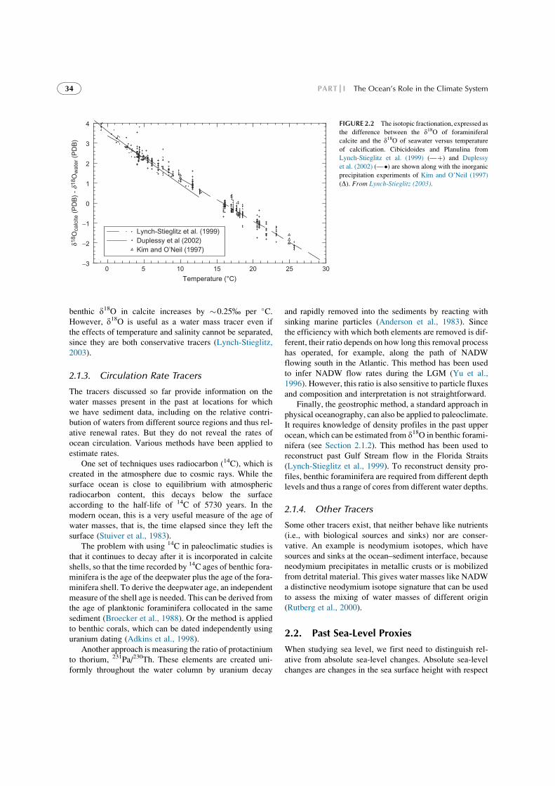
Because of the relatively good availability of data, thelarge climate change signal, and relatively stable climateconditions over several millennia, the LGM was the targetof the earliest proxy reconstructions of paleo-ocean circu-lation (Duplessy et al., 1988) and of a number of time sliceclimate model experiments with atmosphere models, withocean models and with coupled ocean–atmosphere models,including systematic model intercomparison studies(Braconnot et al., 2007a,b). Figure 2.8 (left) shows the dis-tribution of d13C in the modern and LGMAtlantic ocean, asa nutrient-like tracer of water masses (see Section 2.1.1).The d13C distribution of the modern ocean reflects thespread of the well-known water masses NADW andAABW. The LGM Atlantic likewise shows a low-nutrientwater mass of northern origin and below it a high-nutrientwater mass, but their boundary is higher up in the watercolumn at about 2 km depth. The northern water mass issometimes called glacial North Atlantic intermediate water(GNAIW); it can be interpreted as a shoaling of the flow ofNADW which leaves room for a northward and upwardextension of AABW during the LGM. This distributionof water masses was more recently confirmed by Cd/Caratios (Lynch-Stieglitz et al., 2007). More recent anddetailed compilations of LGM proxy data also show apresence of AAIW in the Atlantic, the northward extentof which is subject to ongoing research. d18O data at30 "S from the eastern and western side of the basin indicatea collapse of the east–west density gradient, which currentlycharacterizes the outflow of NADW (see Section 2.1.3).While the protactinium/thorium ratio suggests a NADWrenewal rate similar to today, these d18O data may indicatea much reduced NADW outflow into the Southern Ocean(Lynch-Stieglitz et al., 2007). Reconstructions of surfaceproperties of the northern Atlantic at the same time suggestthat NADW (or GNAIW) formation probably occurred tothe south of the Greenland–Iceland–Scotland ridge duringthe LGM (Oppo and Lehman, 1993; Alley and Clark,

50 40 30 20 10Age (ka)

!125

!100

!75

!50

RS

L (m

)

FIGURE 2.7 Sea-level reconstructions from four different sites (dots

with depth uncertainty bars): New Guinea (blue dots), Sunda Shelf (bluehalf-pluses), Barbados (purple), Bonaparte Gulf (green). The blue and

purple lines show sea-level predictions for New Guinea and Barbados,

while the gray line shows eustatic sea level. The vertical gray bar indicates

the time of the LGM. From Clark et al. (2009).

PART I The Ocean’s Role in the Climate System40

Atl

anti

c o

cean

mo

der

n

NA

DW

Atl

anti

c o

cean

last

gla

cial

max

imu

m"13

C

"13C

0

2500

5000 0

2500

5000

40°S

-0.4

-0.2

+0.2

+0.6

+0.9+1.1

+0.7

+0.9

+0.5

20°S

20°N

40°N

0

65°N

45°N

18

30S

EQ

30N

60N

90N

0 1 2 3 4 5 30S

EQ

30N

Latit

ude

Depth (km)Depth (km)

60N

90N

0 1 2 3 4 5

18

1512

12

63

0

!396

3

0

!1.5

Ice

FIGURE2.8

Left:Distributionof

d13Cinthemod

ernandLGM

AtlanticOcean

from

Dup

lessyetal.(19

88).Right:S

treamfunction

ofAtlanticOcean

circulationformodernandLGM

cond

itions

inthe

clim

atemodel

ofGanop

olskiet

al.(199

8).Darkblue

shadingindicatesbo

ttom

water

ofAntarctic

origin,brow

nthebo

ttom

topography.

1999), consistent with a southward extension of sea icecover and in contrast to the modern ocean where it partlyforms in the Nordic Seas and then overflows this ridge.

The first coupled ocean–atmosphere model simulationof LGM climate (Ganopolski et al., 1998), at the time stillwith prescribed continental ice sheets, produced an LGMcirculation in the Atlantic broadly consistent with theseproxy findings (see Figure 2.8). We can see a southwardshift of deepwater formation, a shoaling of NADW flowand an upward and northward extension of AABW, and asimilar NADW renewal rate as at present, combined witha near-breakdown of the outflow across 30 "S as the over-turning cell recirculates within the Atlantic. This flowpattern is consistent with recent findings of a reversed gra-dient in the 231Pa/230Th ratio between north and southAtlantic during the LGM (Negre et al., 2010).

However, subsequent attempts at modeling LGMclimate, including those for the Paleoclimate ModelingIntercomparison Project, have produced a variety of circu-lation patterns for the LGM Atlantic (Weber et al., 2007).This is perhaps not surprising since the stability propertiesof the thermohaline ocean circulation are highly nonlinearand dependent on a subtle density balance, where particu-larly the freshwater budget is difficult to get right in modelseven for the modern ocean (Hofmann and Rahmstorf,2009). Systematic comparison of model results with the fullsuite of proxy data is needed to establish what range of cir-culation patterns is consistent with the data.

3.2. Abrupt Glacial Climate Changes

While the LGM was a period of frosty climate stabilitylasting for several 1000 years, the glacial time beforethe LGM as well as the period of deglaciation followingthe LGM were rather turbulent, punctuated by abrupt andmassive, large-scale climate changes. An illustration is givenin Figure 2.9, based on Greenland ice core data (often shownas standard because of their high resolution) and sediment

data from the subtropical North Atlantic. The numberedwarm events there are known as Dansgaard–Oeschger(DO) events while H1. . .H6 refers to Heinrich events,defined as episodes of massive continental ice discharge intothe northern Atlantic as documented by ice-rafted debris insediment cores. They could either result from internally orexternally triggered ice sheet instability. Heinrich eventsdo not stand out in Greenland temperature but tend to occurduring cold periods preceding some strong DO events.

There is plentiful and strong evidence linking theseabrupt climate events to changes in Atlantic Ocean circu-lation, reviewed, for example, in Alley (2007). From amechanistic point of view, the perhaps most compellingpiece of evidence for a major role of ocean heat transportchanges is the “bipolar seesaw” (or “seasaw”): an antiphasebehavior between the North Atlantic and the SouthernOcean/Antarctica (Stocker, 1998). Establishing the phaserelationship required accurate relative dating betweendistant paleoclimatic records, which was achieved forGreenland and Antarctic ice cores using the globally syn-chronous variations in atmospheric methane that arerecorded at both poles (Blunier and Brook, 2001;Figure 2.10). Methane changes must be synchronous sincemethane is a well-mixed greenhouse gas in the atmosphere,so they can be used to line up the records. Examination ofthe phase relation shows that during cold phases inGreenland (termed “stadials”) Antarctic temperatureincreases, while at the time of abrupt warming in Greenland(the DO events) Antarctic temperature begins to drop andthen continues to decline during Greenland warm phases(called interstadials).

The same pattern is found in climate model simulationsin response to changes in the Atlantic meridional over-turning circulation (Ganopolski and Rahmstorf, 2001; seeFigure 2.11). This behavior can be nicely explained by asimple conceptualmodel consisting of changes in northwardocean heat transport coupled to a heat reservoir in thesouth, the Southern Ocean (Stocker and Johnsen, 2003).

60 55 50 45 40 35 30 25 20 15 10

16

18

20

22

!42

!40

!38

!36

"18O

(per

mil)

SS

T (

°C)

kyr before present

1

2

345

678

91011

12

13

14151617

YD

Bölling

H1H5 H4 H3 H2H6 ?

H0

FIGURE 2.9 Proxy data from the subtropical Atlantic (green) (Sachs and Lehman, 1999) and from the Greenland ice core GISP2 (blue) (Grootes et al.,

1993) show several Dansgaard–Oeschger (D/O) warm events (numbered). The timing of Heinrich events is marked in red. Gray lines at intervals of

1470 years illustrate the tendency of D/O events to occur with this spacing, or multiples thereof.

PART I The Ocean’s Role in the Climate System42

Subsequent more detailed data, including also millennialevents from the previous glacial period, support thisconcept, showing a magnitude of Antarctic response thatasymptotically approaches an equilibrium with increasingduration of North Atlantic stadials (Margari et al., 2010).

While compelling evidence thus points to ocean heattransport changes at the core of abrupt glacial climateevents, the exact nature of these ocean circulation changesis harder to establish. The simple concept of a bistableAMOC, which is either turned “on” or “off,” clearlydoes not have enough degrees of freedom to explain glacialand modern circulations as well as DO and H events.Neither does the concept of an AMOC that simply hasdifferent flow rates appear to explain the data.For example, why are DOwarmings in Greenland so abrupt?Why do Heinrich events appear as prominent cooling at thePortuguese margin (Cacho et al., 1999) but not in Greenland(Figure 2.9)? And why are DO events associated with a largesalinity increase near Iceland (Kreveld et al., 2000)?

One possible explanation for these features is a conceptwith three distinct circulationmodes and transitions betweenthem (see schematic Figure 2.12), which is based on timeslice reconstructions using sediment cores (Sarntheinet al., 1994) as well as model experiments (Ganopolskiand Rahmstorf, 2001). The central image shows a “coldmode” of the AMOC prevailing during the LGM and stadialperiods. DO events occur when convection starts in theNordic Seas (a situation that is stable in the Holocene butonlymetastable during glacial conditions, that is, in the lattercase the circulation reverts spontaneously to the cold modeafter some hundreds of years), which extends the AMOCnorthward, reduces sea ice cover there, and leads to strongwarming over Greenland. This mechanism can explain thesalinity increase during DO events (Figure 2.11b) and theshape and phasing of Greenland and Antarctic temperatures(Figure 2.11d and e). DO events can thus be viewed as a“flickering” between the Holocene and LGM modes of theAMOC, where the latter is the stable one during glacial

times. Other modeling attempts have been reviewed byKageyama et al. (2010).

Heinrich events can be interpreted as a temporaryshutdown of North Atlantic deepwater formation and flow,caused by a dilution of northern Atlantic surface waters dueto meltwater release stemming from the iceberg dischargeevents (Otto-Bliesner and Brady, 2010). Such a shutdownwould lead to cooling of the North Atlantic (but perhapshardly affecting Greenland, since ocean heat transportalready does not reach that far north in the cold mode)and warming in Antarctica, asymptotically approachingan equilibrium as seen in Figure 2.11e and in ice core data(Margari et al., 2010).

An interesting discussion has arisen about the timingof DO events, many of which tend to occur in intervals

Time (yr)

#Ffw

f(Sv)

NA

DW

(S

v)

(a)

(b)

(c)

(d)

S (

ppt)

#T (

°C)

(e)

1

0.150.120.090.060.03

0

0

31

!7.5!7

!6.5!6

!5.5!5

!18

!16

!14

!12

!10

!8

32

33

34

35

36

10

20

30

40

50

1500 3000 4500 6000 7500 9000

0 1500 3000 4500 6000 7500 9000

0 1500 3000 4500 6000 7500 9000

0 1500 3000 4500 6000 7500 9000

!0.03

2 3

FIGURE 2.11 Simulated DO and Heinrich events. (a) Forcing, (b)

Atlantic overturning, (c) Atlantic salinity at 60 "N, (d) air temperature in

the northern North Atlantic sector (60–70 "N), and (e) temperature overAntarctica (temperature values are given as the difference from the

present-day climate, DT). From Ganopolski and Rahmstorf (2001).

FIGURE 2.10 Oxygen isotopes as a temperature proxy for the Greenland

ice core of GRIP and the Byrd ice core in Antarctica, synchronized on acommon time scale. Graph by A. Ganopolski after (Blunier and Brook,

2001). Heinrich events 4 and 5 are marked as in Figure 2.9.

Chapter 2 Paleoclimatic Ocean Circulation and Sea-Level Changes 43

of 1500 years or multiples thereof (see the gray lines inFigure 2.9; Alley et al., 2001a; Schulz, 2002; Rahmstorf,2003). A physical mechanism that can produce such atiming is stochastic resonance (Gammaitoni et al., 1998;Alley et al., 2001a,b; Ganopolski and Rahmstorf, 2002).Model simulations suggest that solar cycles could providethe weak regular trigger required by the stochastic reso-nance mechanism (Braun et al., 2005).

3.2.1. Deglaciation

Since the late 1990s and based on an increasingly largenumber of proxy records, the time history of deglaciation(the transition from the last ice age into the Holocene)has been interpreted as a globally near synchronouswarming out of the ice age (synchronized in part by theglobal atmospheric CO2 increase), superimposed with a

FIGURE 2.12 Schematic of the three circulation modes explained in the text.

PART I The Ocean’s Role in the Climate System44

north–south seesaw due to episodic changes in the Atlanticoverturning circulation (Alley and Clark, 1999; Clark et al.,2002; Rahmstorf, 2002). During deglaciation, the meltingof the ice sheets may have provided an irregular freshwaterinput disrupting the Atlantic Ocean circulation. The mostrecent data compilations have firmed up that interpretationand added much detail (Barker et al., 2009; Clark et al.,2012). In line with early model results for the response ofthe AMOC to freshwater forcing, they document an imme-diate antiphase response off South Africa and more gradualchanges in Antarctica. Thus, a major role of AMOCchanges in shaping the climate evolution during deglaci-ation can now be considered well established, thanks tothe consistent picture that has emerged from many high-resolution proxy records as well as model simulations.Details of the sequence of events are still subject to activeresearch.

3.3. Glacial Cycles

The prime characteristic of glacial cycles is the growth anddecay of vast continental ice sheets, directly mirrored in theglobal ocean in the form of sea-level and salinity changes.Since the average depth of today’s global ocean is 3790 m,the 130-m sea-level drop during the LGM amounts to!3.5% of all ocean water being removed and stored onland, increasing the average salinity of the remaining oceanwater by over 1 psu and increasing its average d18O contentby 1.0%%0.1% (Clark et al., 2009).

Figure 2.13 shows a reconstruction of eustatic sea-levelchanges over the last four glacial cycles based mainly ond18O and coral data. To first order, it shows a sawtoothpattern with a slow descent into full glacial conditionsbut comparatively rapid deglaciations, which can beexplained by a fundamental asymmetry in ice sheet physics:

continental ice sheets grow slowly by accumulating snow attheir surface, but they can decay muchmore rapidly due to acombination of surface melting and ice flow (i.e., solid icedischarge into the ocean).

Figure 2.14 shows a recent attempt at modeling the lastglacial cycle with an intermediate complexity coupledclimate model driven by variations of the Earth’s orbitalparameters and atmospheric concentration of major green-house gases prescribed from ice core data (Ganopolskiet al., 2010). The model contains a three-dimensional poly-thermal ice sheet model which successfully reproduces thehistory of ice sheet growth and decay and hence sea level,as shown in the figure, with some underestimation of themaximum ice sheet volume. The oscillations superimposedon the basic sawtooth shape result from the precession cyclein the orbital parameters which has a period of 23 kyears.

Age (ka)

2

4

3

1

5.1

5.3 5.

5

7.1

7.3

7.5

8.5

9.1

9.3

9.2

10

12

11

6.5

6.3

6.2

8.2

8.3

RS

L (m

)

Sha

ckle

ton

mea

n w

ater

"18

O (

‰)

0!180

!140

!100

!60

!20

20

60

100 CoralsRohling et al. (1998)Composite RSLShackleton (2000)

50 100 150 200 250 300 350 400 450!1.5

!1.0

!0.5

0.0

0.5

FIGURE 2.13 Left axis: Composite RSL curve (bold gray line) and associated confidence interval (thin gray lines). Crosses: coral reef relative sea-leveldata. Empty circles: Relative sea-level low stands estimated by Rohling et al. (1998). Right axis: variations in mean ocean water d18O derived by

Shackleton (2000) from atmospheric d18O (black line). Graph from Waelbroeck et al. (2002).

Modelled

Corals

?

Waelbroeck et al. (2002)

Time (kyBP)

Sea

leve

l (m

)

120

!140

!120

!100

!80

!60

!40

!20

20

0

110 100 90 80 70 60 50 40 30 20 10 0

FIGURE 2.14 Simulation of the last glacial cycle with the CLIMBER-2ocean–atmosphere ice sheet model compared to the data shown in

Figure 2.13. From Ganopolski et al. (2010).

Chapter 2 Paleoclimatic Ocean Circulation and Sea-Level Changes 45

A remaining challenge is to produce such simulationswith predicted rather than prescribed greenhouse gasconcentrations.

In the course of glacial cycles, ocean circulationchanges have mainly been discussed with respect to abruptevents within the glacial and the specific sequence of eventsduring the last deglaciation (see Section 3.2.1). However, ifa weakening of the Atlantic overturning circulation is ageneral feature of the transitions from glacial to interglacialconditions, due to the massive northern meltwater inputoccurring at these times, then the bipolar seesaw may bepart of the explanation of the time lag of atmosphericcarbon dioxide concentration behind Antarctic temperaturethat is found in Antarctic ice cores (Ganopolski and Roche,2009).

3.4. Interglacial Climates

Conditions during the current Holocene and previous inter-glacials do not differ as dramatically from modern climateas do glacial conditions, so it is more difficult to establishwhat changes in ocean circulation—if any—may haveoccurred. Global mean temperature likely was no more than1.5 "C warmer than in the preindustrial time, if at all,although regional differences were larger (Turney andJones, 2010; McKay et al., 2012). Lynch-Stieglitz et al.(2009) have attempted to reconstruct the flow of the Floridacurrent over the past 8000 years from oxygen isotope dataand found a small increase of 4 Sv (out of a total of!30 Sv)over this period. Given this small change and the uncer-tainties of the proxy method, the main (and also interesting)conclusion probably is that the flow was rather stable overthe last 8000 years.

Most discussion on interglacial climates has focused onsea-level changes, both over the Holocene and in previousinterglacials. Global sea level during the Eemian inter-glacial, !120,000 years BP, has been estimated as peakingat 5.5–9 m above present sea level (Kopp et al., 2009;Dutton and Lambeck, 2012). This is of considerableinterest in the context of current global warming since itmay provide clues about the response of ice sheets towarmer climate conditions. Data from the Eemian in com-bination with an ice sheet model ensemble have been usedto constrain the stability threshold of the Greenland icesheet (Robinson et al., 2011). This threshold could becrossed between 0.8 and 3.2 "C global warming above pre-industrial conditions, with a best estimate of 1.6 "C(Robinson et al., 2012). Discussion on Eemian sea levelcontinues, for example, about sea-level changes withinthe Eemian period and about the relative contributionsof the Greenland and Antarctic ice sheets (Dahl-Jensenet al., 2013).

In theHolocene, sea level is characterized by the long tailof deglaciation due to the long time scale needed for melting

continental ice. Different locations record different timeswhen the relative postglacial sea-level rise ended, due tothe interplay between eustatic sea-level rise and postglacialuplift (or in some places, subsidence). Lambeck et al. (2010)have constructed a eustatic sea-level curve for the past6000 years, based on a multitude of relative sea-level data(Figure 2.15). Their best estimate shows how postglacialsea level rise came to an endbetween2 and3 kyearsBP, afterwhich sea levelwas approximately constant until themodernrise, registered by the tide gauges, started.

A compilation of relative sea-level records for the lasttwo millennia from different parts of the world is shownin Figure 2.16. This shows some consistency but also largelocal deviations (e.g., records for Israel, Cook Islands). It istempting to consider the consistent records as represen-tative of eustatic sea level (the data have already beenadjusted for GIA) while the deviating records are affectedby local issues. More records need to be collected from dif-ferent shores to build up a clearer picture.

Figure 2.17 shows proxy records from the US east coast(also shown in Figure 2.16)with an attempt tomodel the sea-level evolution with a semiempirical model as a function ofglobal temperature. A successful fit is obtained for the lastmillennium but not the time before 1000 AD. Ongoingworksuggests this may be due to the global temperature recon-struction that was used, which is warmer than others before1000 AD and thus leads to sea-level rise in the model at atime when stable sea level is found in the proxy data.

4. THE DEEPER PAST

4.1. Challenges of Deep-TimePaleoceanography

Reconstructing the ocean circulation in the geological pastbecomes increasingly more difficult at earlier times. This ismainlydue to the effects ofplate tectonicswhichcontinuously

Time (ka BP)

Sea

leve

l (m

)

Coral date

Salt-marsh data

Archaeologicaldata

Serpulid data Tid

e ga

uge

7!3

!2.5

!2

!1.5

!1

!0.5

0

0.5

6 5 4 3 2 1 0

FIGURE 2.15 Current best estimates, including uncertainty estimates, ofthe eustatic sea-level change over the past 6000 years, as inferred from geo-

logical and archaeological data and from the tide gauge data for the past

century. From Lambeck et al. (2010).

PART I The Ocean’s Role in the Climate System46

0 500 1000 1500 2000

0 500 1000 1500 2000

0 500 1000 1500 20000 500 1000 1500 2000

0 500 1000 1500 2000

New ZealandGehrels et al. (2008)

NZ

Nova Scotia, CanadaGehrels et al. (2005)

NS

Louisiana, USAGonzalez and Tornqvist (2009)Tornqvist et al. (2004)

LA

North Carolina, USA

NC

CT

0 500 1000 1500 2000

0 500 1000 1500 2000

Connecticut, USAvan de Plassche et al. (1998; dashed lines, grey error) Donnelly et al. (2004; boxes)

0 500 1000 1500 2000

MA

ME

Maine, USAGehrels et al. (2000)

Massachusetts, USADonnelly (2004; dashed lines)This study

GIA = 0.23 mm/yr

GIA = 0.6 mm/yr

GIA = 1 mm/yr (Sand Point) 0.9 mm/yr (Tump Point)

GIA = 1 mm/yr

GIA = 1.7 mm/yr

GIA = 0.4 mm/yr

GIA = 0.4 mm/yr

0 500 1000 1500 2000

IcelandGehrels et al. (2006) GIA = 0.65 mm/yr

IC

NZ

IR

IC

SPNS

NC

MEMACT

LA

0.0

0.2

0.4

0.6

Sea

Lev

el (

m)

Year (AD)

0 500 1000 1500 2000

SpainLeorri et al. (2008a,b)Garcia-Artola et al. (2009)

GIA = 0.25 mm/yr

SP

IT

Southern Cook IslandsGoodwin and Harvey (2008)

CI

CI

GIA = !0.3 mm/yr

Israel - blue boxesSivan et al. (2004)

IR & IT0 500 1000 1500 2000

GIA = 0.6 mm/yr

Italy - open circleLambeck et al. (2004)

Net GIA = 0 mm/yr

Global Tide-GaugesChurch and White (2006)

Jevrejeva et al. (2008)

0 500 1000 1500 2000

FIGURE 2.16 Late Holocene sea-level reconstructions after correction for GIA. Rate applied (listed) was taken from the original publication when

possible. In Israel, land and ocean basin subsidence had a net effect of zero. Reconstructions from salt marshes are shown in blue, archaeological datain green, and coral microatolls in red. Tide gauge data expressed relative to AD 1950–2000 average. Vertical and horizontal scales for all datasets are the

same and are shown for North Carolina. Datasets were vertically aligned for comparison with the summarized North Carolina reconstruction (pink). FromKemp et al. (2011).

0 500 1000 1500 2000

-0.2

0.0

0.2Proxy reconstructions

Model

0 mm/yr +0.6 mm/yr -0.1 mm/yr +2.1

Year (AD)

Rate of sea-level

rise (mm/yr)

Sea

leve

l (m

) Observations (tide gauges)

Sea-level estimates

FIGURE 2.17 Sea-level reconstruction for North Carolina from salt marsh data (as in Figure 2.16, here shown blue) compared to tide gauge data (green)

(Jevrejeva et al., 2006) and a semiempirical model (red). From Kemp et al. (2011).

Chapter 2 Paleoclimatic Ocean Circulation and Sea-Level Changes 47

change the position of continents and the topography of theocean floor on geological timescales, both of which have adirect influence on ocean circulation. In contrast to the oceansin the Quaternary (Section 3), accurate paleogeographicreconstructions are therefore a prerequisite for understandingthe ocean circulation during Earth’s deeper past.

For the past 150 million years or so, paleogeographicreconstructions mostly rely on magnetic anomaliesimprinted into the ocean floor and on the positions of therelatively stable mantle plumes. Unfortunately, theseproxies are not available for earlier times, because oceaniccrust is continuously formed at mid-ocean ridges and laterreturned to the mantle at subduction zones. In fact, theoldest parts of the ocean floor date back to the Jurassicperiod (200–146 million years ago), with the majority beingmuch younger (Muller et al., 2008a; see Figure 2.18). Forearlier times, paleogeographic reconstructions have to relyon paleomagnetic data (indicating the latitude and orien-tation of continents) and paleontological records (indicatingthe geographic distribution of species), making paleogeo-graphic maps increasingly uncertain beyond the Cretaceous(146–66 million years ago) (Cocks and Torsvik, 2002;Torsvik and Cocks, 2004).

The continuous recycling of the oceanic crust also limitsthe sedimentary record and thus the availability of tracers ofpast ocean circulation (see Section 2.2), again making theCretaceous the earliest time for which the physical stateof the ocean can be investigated in detail. As a matter offact, the Cretaceous with its warm greenhouse climateand small meridional temperature gradient is also a partic-ularly interesting period in Earth’s history. In particular, ithas been suggested that the ocean circulation in the Creta-ceous could have been radically different from today. Theremainder of this section therefore concentrates on theclimate during the Cretaceous and briefly reviews researchon the ocean circulation during this time.

4.2. The Oceans During the Mid-CretaceousWarm Period

Temperature reconstructions indicate that the globalaverage surface air temperature was above modern levelsfor the entire Cretaceous, with particularly strong warmingaround 95 million years ago, when global surface airtemperatures were about 20 "C warmer than today(Figure 2.19). In the following, we focus on ocean circu-lation during this mid-Cretaceous warm period, beginningwith a look at the continental configuration at that time.

A reconstruction for the paleogeography during themid-Cretaceous (90 million years ago) is shown inFigure 2.20. At that time, the break-up of the supercontinentPangaea, which had begun in the Jurassic, has progressed toa point where continental landmasses known today hadseparated from each other, although in many cases only

separated by narrow and very shallow seas. Note that thedistribution of continents and the absence or presence ofopen ocean gateways can be of considerable importancefor Earth’s climate. The opening of the passages aroundAntarctica, for example, likely played a major role in thegrowth of its ice sheet and thus for the global and regionalenergy balance (Kennett, 1977).

One particularly striking feature of the geographyduring that period are epicontinental (or epeiric) seas,shallow seas covering large parts of what would laterbecome continental North America, Europe, and Africa.This Cretaceous transgression is thought to be primarilycaused by rapid seafloor spreading at mid-ocean ridges,which reduced the volume of ocean basins and thus ledto a rise in eustatic sea level (Hays and Pitman, 1973). Esti-mates of mid-Cretaceous sea levels differ widely, however,roughly covering a range from 50 to 250 m above presentday (Miller et al., 2005; Muller et al., 2008b).

Early model simulations indicated that the changes inpaleogeography (as compared to present day) alone canaccount for about 5 "C warming during the mid-Cretaceous(Barron and Washington, 1984). Later studies, however,found only a minor contribution to the observed warming(Barron et al., 1995; Bice et al., 2000). Higher levels ofatmospheric greenhouse gases (in particular carbondioxide) are thought to explain the bulk of the warmingduring the Cretaceous.

Mid-Cretaceous atmospheric carbon dioxide levels canbe estimated from proxy data and models of the globalcarbon cycle. Empirical estimates rely on d13C carbonisotope ratios in paleosols, alkenones, or planktonic forami-nifera, distribution of stomatal pores in C3 plants, or d11Bboron isotope ratios in planktonic foraminifera (Royer,2006). As shown in Figure 2.21, atmospheric carbondioxide concentrations during the middle Cretaceous werearound 1000 ppm and thus significantly higher than today,albeit with a large uncertainty range (roughly 500–1500 ppm). A strong contribution of the higher carbondioxide levels (possibly enhanced by methane) to theobserved warming is therefore very likely. The geologicalrecord also indicates an ice-free world during the Jurassicand Cretaceous. These time periods are therefore an idealtestbed to study the internal dynamics of a climate systemwithout polar icecaps.

Concerning geographic patterns, temperature proxydata for the mid-Cretaceous indicate tropical temperaturesa few degrees warmer than today (possibly up to 40 "C), butsignificantly warmer polar regions. As for other warmperiods in Earth’s history, the mid-Cretaceous is thereforecharacterized by a significantly reduced meridional temper-ature gradient often referred to as an “equable” climate(Crowley and Zachos, 2000; Hay, 2008). For illustration,Figure 2.22 shows an example of a proxy-based latitudinaltemperature distribution during the late Cretaceous as

PART I The Ocean’s Role in the Climate System48

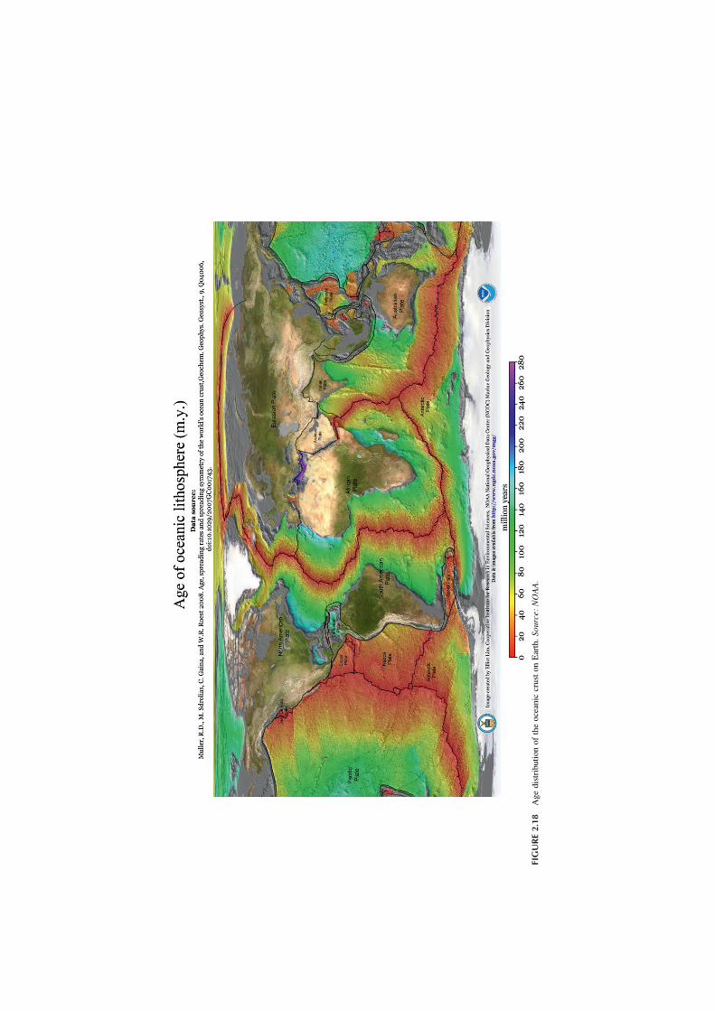
FIGURE2.18

Age

distribution

oftheoceaniccruston

Earth.So

urce:NOAA.

compared to the present-day climate. (Note that earlierstudies had indicated an even flatter Cretaceous temper-ature gradient with “cool tropics,” but this interpretationhas now been shown to be biased by diagenesis, see, e.g.,Pearson et al., 2001).

Equable climates during previous warm periods (and inparticular during the Cretaceous) have received consid-erable attention because climate model experiments havegenerally had difficulties in reproducing the latitudinaltemperature distribution inferred from proxy data

Maas Camp Con Tur Cen Alb Apt Barr Haut Val Berr

70 80 90 100 110 120 130 140

0

10

20

30

40

50

S

Last glacial maximum

Present global average

Tem

perature (°C)

Age in MYA

Cretaceous global average

FIGURE 2.19 Schematic view of reconstructed global surface air temperatures during the Cretaceous. Reproduced from Hay and Floegel (2012).

FIGURE 2.20 Paleogeography (elevation in meters) during the mid-Cretaceous (90 million years ago) in cylindrical (a), North polar (b), and South polar

(c) projections (Sewall et al., 2007).

PART I The Ocean’s Role in the Climate System50

(Crowley and Zachos, 2000). It has often been suggestedthat an increased meridional heat transport in the oceancould have caused the reduced temperature gradient inthe Cretaceous. One hypothesis postulates that—in

contrast to the present-day situation —deepwater for-mation could have taken place at low latitudes, with warmsaline water masses transported at depths toward the poles(Chamberlin, 1906). Model simulations for the Cretaceousdo not support this hypothesis, however, and yield con-flicting results concerning the open ocean sites of deepwaterformation. Emanuel (2001) suggests that the higher intensityof tropical cyclones following an increase in tropical temper-atures could lead to stronger vertical mixing in the tropics,resulting in an increased ocean heat transport toward thepoles. Hotinski and Toggweiler (2003) propose that thepresence of a circumglobal ocean passage at low latitudescould increase the meridional heat transport in the Creta-ceous oceans. This hypothesis is another example of themore general importance of ocean gateways for ocean circu-lation and climate.Hays (2008) argues that a significant con-tribution frommany sources of deepwater along themarginsof the wide-spread shallow seas in the Cretaceous may beexpected. This lack of a truly global overturning circulationcould also help explain the evidence for ocean anoxiaobserved in the sedimentary record as frequent occurrencesof black shales (Hay, 2008).

Clearly,much remains to be done to better understand therole of the ocean circulation for the equable climate problem.However, other factors could have contributed to the shallowtemperature gradient. Forest expansion during in the Creta-ceous has been shown to lead to high-latitude warming, forexample (Otto-Bliesner and Upchurch, 1997; Zhou et al.,2012). Further, an increased meridional transport of latentheat in the atmosphere or changes in the radiative balanceof mid and high latitudes have been suggested to contributeto the equable climate during the Cretaceous. For example,Abbot et al. (2009) suggest a high-latitude positive cloudfeedback mechanism in which high-latitude warming leadsto increased atmospheric convection, resulting in decreasedcooling (or even warming) by clouds at high latitudes andthus a more equable climate. Further, coupled oceanic–atmospheric processes could be important. Rose andFerreira (2013) propose that enhanced ocean heat transportcould drive strong atmospheric convection in the mid-latitudes, leading to warming up to the poles due to higherhumidity in the upper troposphere.

More detailed simulations with coupled Earth systemmodels could shed further light on the processes responsiblefor the equable climate problem and on the role of theoceans in the Cretaceous climate system.

5. OUTLOOK

The proxy data and model results discussed here give animpression of the formidable detective work that is requiredto find and decipher information about past ocean states.Both proxy data and models are difficult and time-consuming to develop and understand, and their resultsare not always easy to interpret. Mistakes and blind alleys

Time (Ma)

0100200300400500

0

2000

4000

6000

8000ProxiesGEOCARB III

(c)

2000

4000

6000

8000Proxies (LOESS)GEOCARB III

(d)

0

CO

2 (p

pm)

CO

2 (p

pm)

CO

2 (p

pm)

0

2000

4000

6000

8000PaleosolsStomataPhytoplanktonBoronLiverworts

(b)

C O S D Carb P Tr J K Pg Ng

Sa

mp

ling

fre

qu

en

cy

0

20

40

60

80(a)

Time (Ma)

0100200300400500

C O S D Carb P Tr J K Pg Ng

FIGURE 2.21 Sampling frequency (panel a) for proxy data for the evo-

lution of atmospheric carbon dioxide concentrations during the Phanerozoic

(the past 542 million years) as shown in panel b. Panel c: comparison of theproxy data (black) with results from carbon cycle modeling (gray, with

uncertainty range). Panel d: comparison of best-guess prediction of the

carbon cycle model (dashed line, range indicated by gray shading) with

the smoothed proxy record (black). Reproduced from Royer (2006).

Chapter 2 Paleoclimatic Ocean Circulation and Sea-Level Changes 51

are an inevitable part of this slow learning process. Yet, wehope we have been able to convince the readers that theseefforts pay off and that slowly, more and more robust andprecise information is emerging. This information aboutpast climate and oceans is crucial for a better understandingof the rapid climate changes we are witnessing (andcausing) at present.

The effort on paleoclimatic research is thus an effortwell spent. While there are still more questions thananswers, there is great promise that further painstakingwork will be able to clarify many of the issues that still seempuzzling today. A better knowledge of the past is vital for animproved understanding of the dynamics of the Earthsystem, and it thus helps to provide the kind of knowledgehumanity needs for a sustainable stewardship of our homeplanet.

ACKNOWLEDGMENTS

We thank Jean Lynch-Stieglitz and Kurt Lambeck for their excellent

review articles, which greatly helped in the preparation of this book

chapter. We also thank Andrew Kemp and Ben Horton for introducing

us to sea-level proxies, and many colleagues, particularly Andrey

Ganopolski, Michael Mann, Eric Steig, and Gavin Schmidt, for

numerous discussions on paleoclimate.

REFERENCES

Abbot, D.S., Huber, M., Bousquet, G., Walker, C.C., 2009. High-CO2

cloud radiative forcing feedback over both land and ocean in a global

climate model. Geophys. Res. Lett. 36, L05702. http://dx.doi.org/

10.1029/2008GL036703.

Adkins, J.F., Cheng, H., Boyle, E.A., Druffel, E.R.M., Edwards, R.L.,

1998. Deep-sea coral evidence for rapid change in ventilation of the

deep North Atlantic 15,400 years ago. Science 280 (5364),

725–728. http://dx.doi.org/10.1126/science.280.5364.725.

Allen, J.R.L., 2000. Morphodynamics of Holocene salt marshes: a review

sketch from the Atlantic and Southern North Sea coasts of Europe.

Quat. Sci. Rev. 19 (12), 1155–1231. http://dx.doi.org/10.1016/

s0277-3791(99)00034-7.

Alley, R.B., 2007. Wally was right: predictive ability of the North Atlantic

“Conveyor belt” hypothesis for abrupt climate change. Annu. Rev.

Earth Planet. Sci. 35, 241–272. http://dx.doi.org/10.1146/annurev.

earth.35.081006.131524, Annual Review of Earth and Planetary

Sciences. Annual Reviews, Palo Alto.

Alley, R.B.,Clark, P.U., 1999. The deglaciation of the northern hemisphere:

a global perspective. Annu. Rev. Earth Planet. Sci. 27, 149–182.

Alley, R.B., Anandakrishnan, S., Jung, P., 2001a. Stochastic resonance in

the North Atlantic. Paleoceanography 16, 190–198.

Alley, R.B., Anandakrishnan, S., Jung, P., Clough, A., 2001b. Stochastic

resonance in the North Atlantic: further insights. In: Seidov, D.,

Maslin, M., Haupt, B.J. (Eds.), The Oceans and Rapid Climate

Change: Past, Present and Future, vol. 126. AGU, Washington,

pp. 57–68, Geophysical Monograph.

Alley, R., et al., 2002. Abrupt Climate Change—Inevitable Surprises.

National Academy Press, Washington, p. 230.

Amiot, R., Lecuyer, C., Buffetaut, E., Fluteau, F., Legendre, S.,

Martineau, F., 2004. Latitudinal temperature gradient during the Cre-

taceous upper Campanian-middle Maastrichtian: d18O record of con-

tinental vertebrates. Earth Planet. Sci. Lett. 226, 255–272. http://dx.

doi.org/10.1016/j.epsl.2004.07.015.

Anderson, R.F.,Bacon,M.P., Brewer, P.G., 1983. Removal of Th-230 and

Pa-231 from the Open Ocean. Earth Planet. Sci. Lett. 62 (1), 7–23.

http://dx.doi.org/10.1016/0012-821x(83)90067-5.

Argus, D.F., Peltier, W.R., 2010. Constraining models of postglacial

rebound using space geodesy: a detailed assessment of model ICE-

5G (VM2) and its relatives. Geophys. J. Int. 181 (2), 697–723.

http://dx.doi.org/10.1111/j.1365-246X.2010.04562.x.

Ballarotta, M., Brodeau, L., Brandefelt, J., Lundberg, P., Doos, K., 2013.

A Last Glacial Maximum world-ocean simulation at eddy-permitting

FIGURE 2.22 Example of a shallow temper-ature gradient during the late Cretaceous: temper-

ature as a function of absolute paleolatitude based

on d18O of fossil continental vertebrates (dashedline) and paleobotanical data (circles) as com-

pared to the present-day gradient (gray line).

Reproduced from Amiot et al. (2004).

PART I The Ocean’s Role in the Climate System52

resolution—part 1: experimental design and basic evaluation. Clim.

Past Discuss. 9, 297–328.

Barker, S., Diz, P., Vautravers, M.J., Pike, J., Knorr, G., Hall, I.R.,

Broecker, W.S., 2009. Interhemispheric Atlantic seesaw response

during the last deglaciation. Nature 457 (7233), 1097–1102. http://

dx.doi.org/10.1038/nature07770.

Barron, E.J., Washington, W.M., 1984. The role of geographic variables

in explaining paleoclimates: results from Cretaceous climate model

sensitivity studies. J. Geophys. Res. 89, 1267–1279.

Barron, E.J., Fawcett, P.J., Peterson, W.H., Pollard, D., Thompson, S.L.,

1995. A “simulation” of mid-Cretaceous climate. Paleoceanography

10, 953–962.

Bice, K.L., Scotese, C.R., Seidov, D., Barron, E.J., 2000. Quantifying the

role of geographic change in Cenozoic ocean heat transport using

uncoupled atmosphere and ocean models. Palaeogeogr. Palaeocli-

matol. Palaeoecol. 161, 295–310.

Blunier, T., Brook, E.J., 2001. Timing of millennial-scale climate change

in Antarctica and Greenland during the last glacial period. Science

291, 109–112.

Boyle, E.A., 1992. Cadmium and delta-C-13 paleochemical ocean distri-

butions during the stage-2 glacial maximum. Annu. Rev. Earth Planet.

Sci. 20, 245–287. http://dx.doi.org/10.1146/annurev.earth.20.1.245.

Boyle, E.A., Sclater, F., Edmond, J.M., 1976. Marine geochemistry of

cadmium. Nature 263 (5572), 42–44. http://dx.doi.org/10.1038/

263042a0.

Braconnot, P., Otto-Bliesner, B., Harrison, S., Joussaume, S.,

Peterchmitt, J.Y., Abe-Ouchi, A., Crucifix, M., Driesschaert, E.,

Fichefet, T., Hewitt, C.D., Kageyama, M., Kitoh, A., Laine, A.,

Loutre, M.F., Marti, O., Merkel, U., Ramstein, G., Valdes, P.,

Weber, S.L., Yu, Y., Zhao, Y., 2007a. Results of PMIP2 coupled sim-

ulations of the mid-Holocene and last glacial maximum—part 1:

experiments and large-scale features. Clim. Past 3 (2), 261–277.

Braconnot, P., Otto-Bliesner, B., Harrison, S., Joussaume, S.,

Peterchmitt, J.Y., Abe-Ouchi, A., Crucifix, M., Driesschaert, E.,

Fichefet, T., Hewitt, C.D., Kageyama, M., Kitoh, A., Loutre, M.F.,

Marti, O., Merkel, U., Ramstein, G., Valdes, P., Weber, L., Yu, Y.,

Zhao, Y., 2007b. Results of PMIP2 coupled simulations of the Mid-

Holocene and Last Glacial Maximum—part 2: feedbacks with

emphasis on the location of the ITCZ and mid- and high latitudes heat

budget. Clim. Past 3 (2), 279–296.

Braun, H., Christl, M., Rahmstorf, S., Ganopolski, A., Mangini, A.,

Kubatzki, C., Roth, K., Kromer, B., 2005. Solar forcing of abrupt glacial

climate change in a coupled climate systemmodel.Nature 438, 208–211.

Broecker, W.S., Andree, M., Bonani, G., Wolfli, W., Oeschger, H.,

Klas, M., Mix, A., Curry, W., 1988. Preliminary estimates for the

radiocarbon age of deep water in the glacial ocean. Paleoceanography

3 (6), 659–669. http://dx.doi.org/10.1029/PA003i006p00659.

Cacho, I., Grimalt, J.O., Pelejero, C., Canals, M., Sierro, F.J., Flores, J.A.,

Shackleton, N.J., 1999. Dansgaard-Oeschger and Heinrich event

imprints in the Alboran Sea paleotemperatures. Paleoceanography

14, 698–705.

Camuffo, D., Sturaro, G., 2003. Sixty-CM submersion of Venice dis-

covered thanks to Canaletto’s paintings. Clim. Change 58 (3),

333–343. http://dx.doi.org/10.1023/a:1023902120717.

Carbognin, L., Teatini, P., Tomasin, A., Tosi, L., 2010. Global change and

relative sea level rise at Venice: what impact in term of flooding. Clim.

Dyn. 35 (6), 1055–1063. http://dx.doi.org/10.1007/s00382-009-0617-5.

Chamberlin, T.C., 1906. On a possible reversal of deep-sea circulation

and its influence on geologic climates. J. Geol. 14, 363–373.

Church, J.A., Woodworth, P.L., Aarup, T., Wilson, W., 2010. Under-

standing Sea-Level Rise and Variability. Blackwell, Oxford.

Clark, P.U., Pisias, N.G., Stocker, T.F., Weaver, A.J., 2002. The role of the

thermohaline circulation in abrupt climate change.Nature 415, 863–869.

Clark, P.U., Dyke, A.S., Shakun, J.D., Carlson, A.E., Clark, J.,

Wohlfarth, B., Mitrovica, J.X., Hostetler, S.W., McCabe, A.M.,

2009. The last glacial maximum. Science 325 (5941), 710–714.

http://dx.doi.org/10.1126/science.1172873.

Clark, P.U., Shakun, J.D., Baker, P.A., Bartlein, P.J., Brewer, S.,

Brook, E., Carlson, A.E., Cheng, H., Kaufman, D.S., Liu, Z.Y.,

Marchitto, T.M., Mix, A.C., Morrill, C., Otto-Bliesner, B.L.,

Pahnke, K., Russell, J.M., Whitlock, C., Adkins, J.F., Blois, J.L.,

Clark, J., Colman, S.M., Curry, W.B., Flower, B.P., He, F.,

Johnson, T.C., Lynch-Stieglitz, J., Markgraf, V., McManus, J.,

Mitrovica, J.X., Moreno, P.I., Williams, J.W., 2012. Global climate

evolution during the last deglaciation. Proc. Natl. Acad. Sci. U.S.A.

109 (19), E1134–E1142. http://dx.doi.org/10.1073/pnas.1116619109.

Claussen, M., et al., 2002. Earth system models of intermediate com-

plexity: closing the gap in the spectrum of climate system models.

Clim. Dyn. 18, 579–586.

Cocks, L.R.M., Torsvik, T.H., 2002. Earth geography from 500 to 400

million years ago: a faunal and palaeomagnetic review. J. Geol.

Soc. 159, 631–644. http://dx.doi.org/10.1144/0016-764901-118.

Crowley, T.J., Zachos, J.C., 2000. Comparison of zonal temperature pro-

files for past warm time periods. In: Huber, B.T., MacLeod, K.G.,

Wing, S.L. (Eds.), Warm Climates in Earth History. Cambridge Uni-

versity Press, Cambridge, UK, pp. 50–76.

Dahl-Jensen, D., Albert, M.R., Aldahan, A., Azuma, N., Balslev-Clausen,

D., Baumgartner, M., Berggren, A.M., Bigler, M., Binder, T., Blunier,

T., Bourgeois, J.C., Brook, E.J., Buchardt, S.L., Buizert, C., Capron,

E., Chappellaz, J., Chung, J., Clausen, H.B., Cvijanovic, I., Davies,

S.M., Ditlevsen, P., Eicher, O., Fischer, H., Fisher, D.A., Fleet, L.

G., Gfeller, G., Gkinis, V., Gogineni, S., Goto-Azuma, K., Grinsted,

A., Gudlaugsdottir, H., Guillevic, M., Hansen, S.B., Hansson, M.,

Hirabayashi, M., Hong, S., Hur, S.D., Huybrechts, P., Hvidberg, C.

S., Iizuka, Y., Jenk, T., Johnsen, S.J., Jones, T.R., Jouzel, J., Karlsson,

N.B., Kawamura, K., Keegan, K., Kettner, E., Kipfstuhl, S., Kjaer, H.

A., Koutnik, M., Kuramoto, T., Kohler, P., Laepple, T., Landais, A.,

Langen, P.L., Larsen, L.B., Leuenberger, D., Leuenberger, M.,

Leuschen, C., Li, J., Lipenkov, V., Martinerie, P., Maselli, O.J.,

Masson-Delmotte, V., McConnell, J.R., Miller, H., Mini, O.,

Miyamoto, A., Montagnat-Rentier, M., Mulvaney, R., Muscheler,

R., Orsi, A.J., Paden, J., Panton, C., Pattyn, F., Petit, J.R., Pol, K.,

Popp, T., Possnert, G., Prie, F., Prokopiou, M., Quiquet, A.,

Rasmussen, S.O., Raynaud, D., Ren, J., Reutenauer, C., Ritz, C.,

Rockmann, T., Rosen, J.L., Rubino, M., Rybak, O., Samyn, D., Sapart,

C.J., Schilt, A., Schmidt, A.M.Z., Schwander, J., Schupbach, S.,

Seierstad, I., Severinghaus, J.P., Sheldon, S., Simonsen, S.B., Sjolte,

J., Solgaard, A.M., Sowers, T., Sperlich, P., Steen-Larsen, H.C.,

Steffen, K., Steffensen, J.P., Steinhage, D., Stocker, T.F., Stowasser,

C., Sturevik, A.S., Sturges, W.T., Sveinbjornsdottir, A., Svensson,

A., Tison, J.L., Uetake, J., Vallelonga, P., van de Wal, R.S.W., van

der Wel, G., Vaughn, B.H., Vinther, B., Waddington, E., Wegner,

A., Weikusat, I., White, J.W.C., Wilhelms, F., Winstrup, M., Witrant,

E., Wolff, E.W., Xiao, C., Zheng, J., 2013. Eemian interglacial

Chapter 2 Paleoclimatic Ocean Circulation and Sea-Level Changes 53

reconstructed from a Greenland folded ice core. Nature 493 (7433),

489–494. http://dx.doi.org/10.1038/nature11789.

Deschamps, P., Durand, N., Bard, E., Hamelin, B., Camoin, G.,

Thomas, A.L., Henderson, G.M., Okuno, J., Yokoyama, Y., 2012.

Ice-sheet collapse and sea-level rise at the Bolling warming

14,600 years ago. Nature 483 (7391), 559–564. http://dx.doi.org/

10.1038/nature10902.

Deuser, W.G., Hunt, J.M., 1969. Stable isotope ratios of dissolved inor-

ganic carbon in Atlantic. Deep Sea Res. 16 (2), 221–225. http://dx.

doi.org/10.1016/0011-7471(69)90078-3.

Donnelly, J.P., Cleary, P., Newby, P., Ettinger, R., 2004. Coupling instru-

mental and geological records of sea-level change: evidence from

southern New England of an increase in the rate of sea-level rise in

the late 19th century. Geophys. Res. Lett. 31, L05203. http://dx.doi.

org/10.1029/2003gl018933.

Duplessy, J.C., Shackleton, N.J., Matthews, R.K., Prell, W.,

Ruddiman,W.F.,Caralp,M.,Hendy,C.H., 1984.C-13recordofbenthic

foraminifera in the last interglacial ocean—implications for the carbon-

cycle and the global deep-water circulation.Quat.Res. 21 (2), 225–243.

http://dx.doi.org/10.1016/0033-5894(84)90099-1.

Duplessy, J.-C., Shackleton, N.J., Fairbanks, R.B., Labeyrie, L., Oppo, D.,

Kallel, N., 1988. Deep water source variations during the last climatic

cycle and their impact on the global deep water circulation. Paleocea-

nography 3, 343–360.

Duplessy, J.C.,Labeyrie, L.,Waelbroeck,C., 2002. Constraints on the ocean

oxygen isotopic enrichment between the last glacial maximum and the

Holocene: paleoceanographic implications. Quat. Sci. Rev. 21 (1–3),

315–330. http://dx.doi.org/10.1016/s0277-3791(01)00107-x.

Dutton, A., Lambeck, K., 2012. Ice volume and sea level during the last

interglacial. Science 337 (6091), 216–219. http://dx.doi.org/10.1126/

science.1205749.

Elderfield, H., Rickaby, R.E.M., 2000. Oceanic Cd/P ratio and nutrient

utilization in the glacial Southern ocean. Nature 405 (6784),

305–310. http://dx.doi.org/10.1038/35012507.

Emanuel, K., 2001. Contribution of tropical cyclones to meridional heat

transport by the oceans. J. Geophys. Res. 106, 14771–14781. http://

dx.doi.org/10.1029/2000JD900641.

Fairbanks, R.G., 1989. A 17,000-year glacio-eustatic sea level record:

influence of glacial melting rates on the younger Dryas event and

deep-ocean circulation. Nature 342, 637–642.

Fichefet, T., Hovine, S., Duplessy, J.C., 1994. A model study of the

Atlantic thermohaline circulation during the last glacial maximum.

Nature 372, 252–255.

Gammaitoni, L., Hanggi, P., Jung, P., Marchesoni, F., 1998. Stochastic

resonance. Rev. Mod. Phys. 70, 223–287.

Ganopolski, A., Rahmstorf, S., 2001. Rapid changes of glacial climate

simulated in a coupled climate model. Nature 409, 153–158.

Ganopolski, A., Rahmstorf, S., 2002. Abrupt glacial climate changes due

to stochastic resonance. Phys. Rev. Lett. 88 (3), 038501.

Ganopolski, A.,Roche,D.M., 2009.On the nature of lead–lag relationships

during glacial–interglacial climate transitions. Quat. Sci. Rev. 28,

3361–3378. http://dx.doi.org/10.1016/j.quascirev.2009.09.019.

Ganopolski, A., Rahmstorf, S., Petoukhov, V., Claussen, M., 1998. Sim-

ulation of modern and glacial climates with a coupled global model of

intermediate complexity. Nature 391, 351–356.

Ganopolski, A., Calov, R., Claussen, M., 2010. Simulation of the last

glacial cycle with a coupled climate ice-sheet model of intermediate

complexity. Clim. Past 6 (2), 229–244.

Gehrels, W.R., 1994. Determining relative sea-level change from salt-

marsh foraminifera and plant zones on the coast of Maine, USA. J.

Coast. Res. 10 (4), 990–1009.

Grinsted,A.,Moore, J.C., Jevrejeva, S., 2010. Reconstructing sea level from

paleo and projected temperatures 200 to 2100 AD. Clim. Dyn. 34,

461–472. http://dx.doi.org/10.1007/s00382-008-0507-2.

Grootes, P.M., Stuiver, M., White, J.W.C., Johnsen, S., Jouzel, J., 1993.

Comparison of oxygen isotope records from the GISP2 and GRIP

Greenland ice cores. Nature 366, 552–554.

Hay, W.W., 2008. Evolving ideas about the Cretaceous climate and ocean

circulation. Cretaceous Res. 29, 725–753. http://dx.doi.org/10.1016/j.

cretres.2008.05.025.

Hay,W.W., Floegel, S., 2012. New thoughts about the Cretaceous climate

and oceans. Earth Sci. Rev. 115, 262–272. http://dx.doi.org/10.1016/j.

earscirev.2012.09.008.

Hays, J.D., Pitman, W.C., 1973. Lithospheric plate motion, sea level

changes and climatic and ecological consequences. Nature 246,

18–22. http://dx.doi.org/10.1038/246018a0.

Hesse, T., Butzin, M., Bickert, T., Lohmann, G., 2011. A model-data com-

parison of delta C-13 in the glacial Atlantic Ocean. Paleoceanography

26, 16. http://dx.doi.org/10.1029/2010pa002085.

Hofmann, M., Rahmstorf, S., 2009. On the stability of the

Atlantic meridional overturning circulation. Proc. Natl. Acad. Sci.

U.S.A. 106 (49), 20584–20589. http://dx.doi.org/10.1073/pnas.

0909146106.

Hotinski, R.M., Toggweiler, J.R., 2003. Impact of a Tethyan circumglobal

passage on ocean heat transport and “equable” climates. Paleoceano-

graphy 18, 1007. http://dx.doi.org/10.1029/2001PA000730.

Jevrejeva, S., Grinsted, A., Moore, J.C., Holgate, S., 2006. Nonlinear

trends and multiyear cycles in sea level records. J. Geophys. Res.

111, C09012. http://dx.doi.org/10.1029/2005JC003229.

Kageyama, M., Paul, A., Roche, D.M., Van Meerbeeck, C.J., 2010.

Modelling glacial climatic millennial-scale variability related to

changes in the Atlantic meridional overturning circulation: a review.

Quat. Sci. Rev. 29 (21–22), 2931–2956. http://dx.doi.org/10.1016/

j.quascirev.2010.05.029.

Kemp, A., Horton, B., Donnelly, J., Mann, M.E., Vermeer, M.,

Rahmstorf, S., 2011. Climate related sea-level variations over the past

two millennia. Proc. Natl. Acad. Sci. U.S.A. 108 (27), 11017–11022.

http://dx.doi.org/10.1073/pnas.1015619108.

Kennett, J.P., 1977. Cenozoic evolution of Antarctic glaciation, the

circum-Antarctic ocean, and their impact on global paleoceanography.

J. Geophys. Res. 82, 3843–3860. http://dx.doi.org/10.1029/

JC082i027p03843.

Kim, S.T., O’Neil, J.R., 1997. Equilibrium and non-equilibrium oxygen

isotope effects in synthetic carbonates. Geochim. Cosmochim. Acta

61, 3461–3475.

Kopp, R.E., Simons, F.J., Mitrovica, J.X., Maloof, A.C.,

Oppenheimer, M., 2009. Probabilistic assessment of sea level during

the last interglacial stage. Nature 462 (7275), 863–867. http://dx.doi.

org/10.1038/nature08686.

Kreveld, S.V., Sarnthein, M., Erlenkeuser, H., Grootes, P., Jung, S.,

Nadeau, M.J., Pflaumann, U., Voelker, A., 2000. Potential links

between surging ice sheets, circulation changes, and the Dansgaard-

Oeschger cycles in the Irminger Sea, 60-18 kyr. Paleoceanography

15, 425–442.

Lambeck, K., 2002. Sea-level change from mid-Holocene to recent time:

an Australian example with global implications. In: Mitrovica, J.X.,

PART I The Ocean’s Role in the Climate System54

Vermeersen, L. (Eds.), Glacial Isostatic Adjustment and the Earth

System. AGU, Washington, pp. 33–50.

Lambeck, K., Bard, E., 2000. Sea-level change along the French Mediter-

ranean coast for the past 30 000 years. Earth Planet. Sci. Lett. 175

(3–4), 203–222. http://dx.doi.org/10.1016/s0012-821x(99)00289-7.

Lambeck, K., Anzidei, M., Antonioli, F., Benini, A., Espositol, A., 2004.

Sea level in Roman times in the central Mediterranean and implica-

tions for recent change. Earth Planet. Sci. Lett. 224, 563–575.

Lambeck, K., Woodroffe, C., Antonioli, F., Anzidei, M., Gehrels, W.R.,

Laborel, J., Wright, A.J., 2010. Paeoenvironmental records, geo-

physical modeling, and reconstruction of sea-level trends and vari-

ability on centennial and longer time scales. In: Church, J.A.,

Woodworth, P.L., Aarup, T., Wilson, W. (Eds.), Understanding Sea-

Level Rise and Variability. Blackwell, Oxford, pp. 61–121.

Lisiecki, L.E., Raymo, M.E., 2005. A Pliocene-Pleistocene stack of 57

globally distributed benthic delta O-18 records. Paleoceanography

20, Pa1003. http://dx.doi.org/10.1029/2004pa001071.

Lyell, C., 1832. Principles of Geology. Murray, London.

Lynch-Stieglitz, J., 2003. Tracers of past ocean circulation. In:

Turkekian, K., Holland, H. (Eds.), Treatise on Geochemistry, vol. 6.

Elsevier, pp. 433–451.

Lynch-Stieglitz, J., Curry, W.B., Slowey, N., 1999. A geostrophic

transport estimate for the Florida current from the oxygen isotope com-

position of benthic foraminifera. Paleoceanography 14 (3), 360–373.

http://dx.doi.org/10.1029/1999pa900001.

Lynch-Stieglitz, J., Adkins, J.F., Curry, W.B., Dokken, T., Hall, I.R.,

Herguera, J.C., Hirschi, J.J.M., Ivanova, E.V., Kissel, C.,

Marchal, O., Marchitto, T.M., McCave, I.N., McManus, J.F.,

Mulitza, S., Ninnemann, U., Peeters, F., Yu, E.F., Zahn, R., 2007.

Atlantic meridional overturning circulation during the last glacial

maximum. Science 316 (5821), 66–69. http://dx.doi.org/10.1126/

science.1137127.

Lynch-Stieglitz, J., Curry, W.B., Lund, D.C., 2009. Florida Straits density

structure and transport over the last 8000 years. Paleoceanography 24,

9. http://dx.doi.org/10.1029/2008pa001717.

Margari, V., Skinner, L.C., Tzedakis, P.C., Ganopolski, A.,

Vautravers, M., Shackleton, N.J., 2010. The nature of millennial-scale

climate variability during the past two glacial periods. Nat. Geosci. 3

(2), 127–131. http://dx.doi.org/10.1038/ngeo740.

McCulloch, M.T., Tudhope, A.W., Esat, T.M., Mortimer, G.E.,

Chappell, J., Pillans, B., Chivas, A.R., Omura, A., 1999. Coral record

of equatorial sea-surface temperatures during the penultimate deglaci-

ation at Huon Peninsula. Science 283 (5399), 202–204. http://dx.doi.

org/10.1126/science.283.5399.202.

McKay, N.P.,Overpeck, J.T., Otto-Bliesner, B.L., 2012. The role of ocean

thermal expansion in last interglacial sea level rise. Geophys. Res.

Lett. 38, L14605. http://dx.doi.org/10.1029/2011gl048280.

Milankovitch,M., 1941. Kanon der Erdbestrahlung und seine Anwendung

auf das Eiszeitenproblem. Koniglich Serbische Akademie, Belgrad.

Miller, K.G., Kominz, M.A., Browning, J.V., Wright, J.D.,

Mountain, G.S., Katz, M.E., Sugarman, P.J., Cramer, B.S.,

Christie-Blick, N., Pekar, S.F., 2005. The phanerozoic record of global

sea-level change. Science 310, 1293–1298. http://dx.doi.org/10.1126/

science.1116412.

Muller, R.D., Sdrolias, M., Gaina, C., Roest, W.R., 2008a. Age, spreading

rates, and spreading asymmetry of the world’s ocean crust. Geochem.

Geophys. Geosyst. 9, Q04006. http://dx.doi.org/10.1029/2007

GC001743.

Muller, R.D., Sdrolias, M., Gaina, C., Steinberger, B., Heine, C.,

2008b. Long-term sea-level fluctuations driven by ocean basin

dynamics. Science 319, 1357–1362. http://dx.doi.org/10.1126/

science.1151540.

Negre, C., Zahn, R., Thomas, A.L., Masque, P., Henderson, G.M.,

Martinez-Mendez, G., Hall, I.R., Mas, J.L., 2010. Reversed flow of

Atlantic deep water during the last glacial maximum. Nature 468

(7320), 84. http://dx.doi.org/10.1038/nature09508.

Oppo, D., Lehman, S.J., 1993. Mid-depth circulation of the subpolar

North Atlantic during the last glacial maximum. Science 259,

1148–1152.

Ota, Y., Chappell, J., 1999. Holocene sea-level rise and coral reef growth

on a tectonically rising coast, Huon Peninsula, Papua New Guinea.

Quat. Int. 55, 51–59. http://dx.doi.org/10.1016/s1040-6182(98)

00024-x.

Otto-Bliesner, B.L., Brady, E.C., 2010. The sensitivity of the climate

response to the magnitude and location of freshwater forcing: last

glacial maximum experiments. Quat. Sci. Rev. 29 (1–2), 56–73.

http://dx.doi.org/10.1016/j.quascirev.2009.07.004.

Otto-Bliesner, B.L., Upchurch Jr., G.R., 1997. Vegetation-induced

warming of high-latitude regions during the late Cretaceous period.

Nature 385, 804–807.

Passaro, S., Barra, M., Saggiomo, R., Di Giacomo, S., Leotta, A.,

Uhlen, H., Mazzola, S., 2013. Multi-resolution morpho-bathymetric

survey results at the Pozzuoli-Baia underwater archaeological site

(Naples, Italy). J. Archaeol. Sci. 40 (2), 1268–1278. http://dx.doi.

org/10.1016/j.jas.2012.09.035.

Pearson, P.N., Ditchfield, P.W., Singano, J., Harcourt-Brown, K.G.,

Nicholas, C.J., Olsson, R.K., Shackleton, N.J., Hall, M.A., 2001.

Warm tropical sea surface temperatures in the late Cretaceous and

Eocene epochs. Nature 413, 481–487. http://dx.doi.org/10.1038/

413481A0.

Peltier, W.R., Fairbanks, R.G., 2006. Global glacial ice volume and last

glacial maximum duration from an extended Barbados sea level

record. Quat. Sci. Rev. 25 (23–24), 3322–3337. http://dx.doi.org/

10.1016/j.quascirev.2006.04.010.

Pirazzoli, P.A., Evelpidou, N., 2013. Tidal notches: a sea-level indicator of

uncertain archival trustworthiness. Palaeogeogr. Palaeoclimatol.

Palaeoecol. 369, 377–384. http://dx.doi.org/10.1016/j.palaeo.2012.11.

004.

Rahmstorf, S., 2002. Ocean circulation and climate during the past

120,000 years. Nature 419, 207–214.

Rahmstorf, S., 2003. Timing of abrupt climate change: a precise clock.

Geophys. Res. Lett. 30, 1510.

Rahmstorf, S., 2007. A semi-empirical approach to projecting future sea-

level rise. Science 315 (5810), 368–370.

Robinson, A., Calov, R., Ganopolski, A., 2011. Greenland ice sheet

model parameters constrained using simulations of the Eemian Inter-

glacial. Clim. Past 7 (2), 381–396. http://dx.doi.org/10.5194/cp-7-

381-2011.

Robinson, A., Calov, R., Ganopolski, A., 2012. Multistability and critical

thresholds of the Greenland ice sheet. Nat. Clim. Chang. 2 (6),

429–432. http://dx.doi.org/10.1038/nclimate1449.

Rohling, E.J., Fenton, M., Jorissen, F.J., Bertrand, P., Ganssen, G.,

Caulet, J.P., 1998. Magnitudes of sea-level lowstands of the past

500,000 years. Nature 394, 162–165. http://dx.doi.org/10.1038/28134.

Rose, B.E.J., Ferreira, D., 2013. Ocean heat transport and water vapor

greenhouse in a warm equable climate: a new look at the low gradient

Chapter 2 Paleoclimatic Ocean Circulation and Sea-Level Changes 55

paradox. J. Clim. 26, 2117–2136. http://dx.doi.org/10.1175/JCLI-D-

11-00547.1.

Rosenthal, Y., Boyle, E.A., Slowey, N., 1997. Temperature control on the

incorporation of magnesium, strontium, fluorine, and cadmium into

benthic foraminiferal shells from Little Bahama Bank: prospects for

thermocline paleoceanography. Geochim. Cosmochim. Acta 61

(17), 3633–3643. http://dx.doi.org/10.1016/s0016-7037(97)00181-6.

Royer, D.L., 2006. CO2-forced climate thresholds during the Phanerozoic.

Geochim. Cosmochim. Acta 70, 5665–5675. http://dx.doi.org/

10.1016/j.gca.2005.11.031.

Ruddiman, W.F., 2000. Earths Climate: Past and Future. Freeman, New

York, p. 465.

Rutberg, R.L., Hemming, S.R., Goldstein, S.L., 2000. Reduced North

Atlantic deep water flux to the glacial Southern ocean inferred from

neodymium isotope ratios. Nature 405 (6789), 935–938.

Sachs, J.P., Lehman, S.J., 1999. Subtropical North Atlantic temperatures

60,000 to 30,000 years ago. Science 286, 756–759.

Sarnthein, M., Winn, K., Jung, S.J.A., Duplessy, J.C., Labeyrie, L.,

Erlenkeuser, H., Ganssen, G., 1994. Changes in east Atlantic deep-

water circulation over the last 30,000 years: eight time slice recon-

structions. Paleoceanography 9, 209–267.

Schmidt, G.A., 1999. Forward modeling of carbonate proxy data from

planktonic foraminifera using oxygen isotope tracers in a global ocean

model. Paleoceanography 14 (4), 482–497. http://dx.doi.org/10.1029/

1999pa900025.

Schrag, D.P., Adkins, J.F., McIntyre, K., Alexander, J.L., Hodell, D.A.,

Charles, C.D., McManus, J.F., 2002. The oxygen isotopic composition

of seawater during the last glacial maximum. Quat. Sci. Rev. 21 (1–3),

331–342. http://dx.doi.org/10.1016/s0277-3791(01)00110-x.

Schulz, M., 2002. On the 1470-year pacing of Dansgaard-Oeschger warm

events. Paleoceanography 17, 4-1–4-9.

Scott, D.S.,Medioli, F.S., 1978. Vertical zonations of Marsh foraminifera

as accurate indicators of former sea-levels. Nature 272 (5653),

528–531. http://dx.doi.org/10.1038/272528a0.

Sewall, J.O., van de Wal, R.S.W., van der Zwan, K., van Oosterhout, C.,

Dijkstra, H.A., Scotese, C.R., 2007. Climate model boundary condi-

tions for four Cretaceous time slices. Clim. Past 3, 647–657. http://

dx.doi.org/10.5194/cp-3-647-2007.

Shackleton,N.J., 2000. The 100,000-year ice-age cycle identified and found

to lag temperature, carbon dioxide, and orbital eccentricity. Science 289,

1897–1902. http://dx.doi.org/10.1126/science.289.5486.1897.

Shennan, I., et al., 2007. Sea level studies. In: In: Elias, S.A. (Ed.), Ency-

clopedia of Quaternary Science, vol. 4. Elsevier, Amsterdam,

pp. 2967–3095.

Sivan, D., Lambeck, K., Toueg, R., Raban, A., Porath, Y., Shirman, B.,

2004. Ancient coastal wells of Caesarea Maritima, Israel, an indicator

for relative sea level changes during the last 2000 years. Earth Planet.

Sci. Lett. 222 (1), 315–330. http://dx.doi.org/10.1016/j.epsl.2004.

02.007.

Spero, H.J., Lea, D.W., 1996. Experimental determination of stable

isotope variability in Globigerina bulloides: implications for paleocea-

nographic reconstructions. Mar. Micropaleontol. 28 (3–4), 231–246.

http://dx.doi.org/10.1016/0377-8398(96)00003-5.

Stanford, J.D., Rohling, E.J., Hunter, S.E., Roberts, A.P., Rasmussen, S.O.,

Bard, E., McManus, J., Fairbanks, R.G., 2006. Timing of meltwater

pulse 1a and climate responses to meltwater injections. Paleoceano-

graphy 21, Pa4103. http://dx.doi.org/10.1029/2006pa001340.

Stanley, S., 2005. Earth SystemHistory.W.H. Freeman, NewYork, p. 567.

Stocker, T.F., 1998. The seesaw effect. Science 282, 61–62.

Stocker, T.F., Johnsen, S.J., 2003. A minimum thermodynamic model for

the bipolar seesaw. Paleoceanography 18, art. no. 1087 http://online-

library.wiley.com/http://dx.doi.org/10.1029/2003PA000920/abstract.

Stuiver, M., Quay, P.D., Ostlund, H.G., 1983. Abyssal water C-14 distri-

bution and the age of the world oceans. Science 219 (4586), 849–851.

http://dx.doi.org/10.1126/science.219.4586.849.

Tachikawa, K., Elderfield, H., 2002. Microhabitat effects on Cd/Ca and

delta C-13 of benthic foraminifera. Earth Planet. Sci. Lett. 202 (3–4),

607–624. http://dx.doi.org/10.1016/s0012-821x(02)00796-3.

Torsvik, T.H.,Cocks, L.R.M., 2004. Earth geography from 400 to 250Ma:

a palaeomagnetic, faunal and facies review. J. Geol. Soc. 161,

555–572. http://dx.doi.org/10.1144/0016-764903-098.

Turney, C.S.M., Jones, R.T., 2010. Does the Agulhas current amplify

global temperatures during super-interglacials? J. Quat. Sci. 25 (6),

839–843. http://dx.doi.org/10.1002/jqs.1423.

Waelbroeck, C., Labeyrie, L., Michel, E., Duplessy, J.C., McManus, J.F.,

Lambeck, K., Balbon, E., Labracherie, M., 2002. Sea-level and deep

water temperature changes derived from benthic foraminifera isotopic

records. Quat. Sci. Rev. 21 (1–3), 295–305.

Weber, S.L., Drijfhout, S.S., Abe-Ouchi, A., Crucifix, M., Eby, M.,

Ganopolski, A., Murakami, S., Otto-Bliesner, B., Peltier, W.R.,

2007. The modern and glacial overturning circulation in the Atlantic

Ocean in PMIP coupled model simulations. Clim. Past 3 (1), 51–64.

Wefer, G., Berger, W.H., 1991. Isotope paleontology—growth and com-

position of extant Calcareous species. Mar. Geol. 100 (1–4), 207–248.

http://dx.doi.org/10.1016/0025-3227(91)90234-u.

Woodroffe, C.,McLean, R., 1990.Microatolls and recent sea-level change

on coral atolls. Nature 344 (6266), 531–534. http://dx.doi.org/10.1038/

344531a0.

Yu, E.-F., Francois, R., Bacon, M.P., 1996. Similar rates of modern and

last-glacial ocean thermohaline circulation inferred from radio-

chemical data. Nature 379, 689–694.

Zhou, J., Poulsen, C.J., Rosenbloom, N., Shields, C., Briegleb, B., 2012.

Vegetation-climate interactions in the warm mid-Cretaceous. Clim.

Past 8, 565–576. http://dx.doi.org/10.5194/cp-8-565-2012.

PART I The Ocean’s Role in the Climate System56