PADRÕES DE DIVERSIDADE DE AVES E REDE DE INTERAÇÃO

UNIVERSIDADE FEDERAL DO RIO GRANDE DO SUL

INSTITUTO DE BIOCIÊNCIAS

PROGRAMA DE PÓS-GRADUAÇÃO EM ECOLOGIA

TESE DE DOUTORADO

GRASIELA CASAS

PADRÕES DE DIVERSIDADE DE AVES E REDE DE INTERAÇÃO

MUTUALÍSTICA AVE-PLANTA EM MOSAICO FLORESTA-CAMPO

PORTO ALEGRE, AGOSTO DE 2015

II

PADRÕES DE DIVERSIDADE DE AVES E REDE DE INTERAÇÃO

MUTUALÍSTICA AVE-PLANTA EM MOSAICO FLORESTA-CAMPO

GRASIELA CASAS

TESE DE DOUTORADO APRESENTADA AO

PROGRAMA DE PÓS-GRADUAÇÃO EM

ECOLOGIA, DO INSTITUTO DE

BIOCIÊNCIAS DA UNIVERSIDADE

FEDERAL DO RIO GRANDE DO SUL, COMO

PARTE DOS REQUISITOS PARA OBTENÇÃO

DO TÍTULO DE DOUTOR EM ECOLOGIA.

Orientador: Prof. Dr. Valério De Patta

Pillar

Comissão Examinadora:

Prof. Dr. Leandro Bugoni

Prof. Dr. Gerhard Ernst Overbeck

Prof. Dr. Milton de Souza Mendonça

Júnior

PORTO ALEGRE, AGOSTO DE 2015

III

“Um dia, a menina observando andorinhas a bailar, com os pés no chão e uma pena

na mão, queria voar. Então, ela tomou uma decisão: nunca parar de estudar. Hoje,

com sonhos nas mãos e entre livros, artigos, amigos e estórias, não se cansa de

migrar.

Mas por hoje chega de prosa, porque não dá para parar! A menina sem penas

continua querendo voar e voar…”

Grasiela Casas

IV

AGRADECIMENTOS

Foram quatro anos de muito aprendizado, trabalho, diversão, erros (muitos

erros) e consequentemente muito crescimento. Finalizar o doutorado para mim não é

somente uma etapa na carreira profissional, mas também a realização de um sonho de

quem há muitos anos considerava a graduação quase impossível. Ainda bem que tinha

um “quase” que me fez chegar até aqui. Por isto, gostaria de agradecer a todos que

participaram desta etapa, seja me ajudando em campo, amigas (os) que me ajudaram

nos momentos difíceis e que também me acompanharam nas festas, à família, aos

proprietários que permitiram “a menina das aves” entrar em suas propriedades na

madrugada, aos professores e instituições. Muito obrigada!

Primeiramente, gostaria de agradecer meu orientador Valério De Patta Pillar por

aceitar me orientar, pela confiança e contribuições. És um exemplo de profissional.

Também gostaria de agradecer à Sandra C. Muller, minha co-orientadora não oficial

do doutorado, que desde o mestrado continuou me aconselhando e me ajudando. Me

inspiro em ti como Mulher na ciência. Um dia chego lá.

Ao Neo Martinez, que gentilmente me aceitou no doutorado sanduíche no

Pacific Ecoinformatics and Computational Ecology Lab, mesmo a minha proposta

não sendo a linha de pesquisa principal de seu laboratório. À Fernanda Valdovinos,

posdoc que também participou das discussões dos meus dados com o professor Neo.

Às maravilhosas bolsistas Cristiane Alves da Silva, Pâmela Friedemann e

Danielle Franco. À Cris, que participou em quase todas as marcações das áreas e

pontos de escuta, mesmo entrando em várias “frias”, dirigindo comigo na madrugada

de uma cidade para outra. À Pâmela, que com sua paciência e dedicação fez o

trabalho mais pesado das sementes. À Dani, que fez grande parte das medições das

V

aves nos museus. Gurias, sem vocês meu doutorado teria sido mais trabalhoso e com

certeza, menos divertido.

A todos os ajudantes de campo, principalmente nas redes de neblina, como a

Pâmela Friedemann e Danielle Franco (quase todas as saídas), Cristiane Alves e

Giuliano Brusco (em muitas), Adriano Machado, Iporã da Silva Haeser, Voltaire

Paes, Ângelo Marcon, Gustavo K. Santos, Martin Sucunza, Camila Dias, Diogenes B.

Machado, Felipe Zílio, André Luis P. Dresseno, Amanda Aguiar, Kevin Ortiz, Tiago

F. Steffen, João P. Langhans, Paulo Barradas, Carolina Prauchner, Pedro M.A.

Ferreira, Mariana Lopes, Karine Costa, Antônio Dos Santos Jr., Humberto Mohr,

Felícia Fischer, Morten Hemp, Laura Cappelatti, Rodrigo Pettini, Poliana de Paula,

Karine D. de Lima, Mateus Camana, Fabrício Orellna L. e Pricila Lopes.

Ao Vinícius Bastazini, que me iniciou no mundo das análises de redes e

continua enviando artigos. Ao Vanderlei Debastiani, pelo entusiasmo e programação

no R para o terceiro capítulo. Sem vocês dois o último capítulo da tese não teria

saído!

Ao Pedro M. A. Ferreira, pelo companheirismo, carinho, paciência e toda ajuda

não oficial durante o doutorado. Cresci muito ao teu lado nestes anos juntos.

A todos os colegas do Ecoqua, pelas parcerias, carinho e momentos

maravilhosos: Bethânia Azambuja, Anaclara Guido, Letícia Dadalt, Kátia Zanini,

Omara Lange, Felícia Fischer, Rafael Machado, Carolina Blanco, Vasiliki Balogianni,

Bianca Darski e Rodrigo Baggio. Ao Eduardo Vélez, um dos integrantes

fundamentais do projeto SISBIOTA (biodiversidade dos campos e dos ecótonos

campo-floresta no Sul do Brasil: bases ecológicas para sua conservação e uso

sustentável), pelos mapas das áreas e maravilhosas festas de aniversário!

VI

À Mariana Gliesch Silva e Rodrigo Bergamin pelos dados fitossociológicos das

áreas de ecótono do projeto SISBIOTA, e junto com Kátia Zanini, pelos atributos das

plantas.

Aos botânicos Martin Molz, Rodrigo Bergamin, Marcos Carlucci, Guilherme

Seger, Fernanda Schimidt e Ari D. Nilson pela grande ajuda na identificação das

plantas coletadas, principalmente ao Martin Molz. Ao Herbário ICN (Herbário do

Instituto de Biociências, Universidade Federal do Rio Grande do Sul), que nos

permitiu abrir alguns frutos dos exemplares das exsicatas.

Aos vários integrantes do projeto SISBIOTA e aos que também marcaram as

áreas de ecótono, como André L. Luza, Marcos Carlucci, Rodrigo Bergamin, Mariana

Gliesch Silva e Carolina Blanco.

À Bethania Azambuja, Rômulo Vitória e Adriano Scherer por terem

disponibilizado seus dados de interação. Obrigada pela confiança.

Aos meus eternos mestres ornitólogos, André Mendonça Lima, Jan Karel e

Felipe Zílio, pelos vários papos e sugestões. Principalmente ao André, que ajudou

com a burocracia do anilhamento quando eu não era anilhadora sênior. Também ao

Rafael Dias, que mediu algumas das aves nas coleções pelo projeto SISBIOTA e

disponibilizou os dados.

Ao proprietários das áreas pela autorização, carinho e confiança: Geraldo

Mastrantônio, Bertília e netos (Herval); Affonso Mibieli e Mirna (Encruzilhada do

Sul); Leni Krusser, esposa e filha, e Carlão (Santana da Boa Vista); Martim Antônio

da Cunha e gestora da APA do Ibirapuitã, Eridiane L. da Silva (Santana do

Livramento); José Carlos Medeiros, Albino e Paulo Funk (São Francisco de Assis);

Teófilo Garcia (Santo Antônio das Missões); SEMA São Francisco de Paula,

principalmente ao gestor Daniel Slomp, Fabiana P. Bertuol, e aos proprietários que

VII

nos deram acesso ao PE Tainhas, como Jane Santos, José Carlos Almeida e Zizi

(Jaquirana); IcMbio (Instituto Chico Mendes de Conservação da Biodiversidade),

PARNA Aparados da Serra, principalmente ao gestor Deonir e Lúcio M. dos Santos

(Cambará do Sul); CPCN Pró-Mata (São Francisco de Paula).

Ao Museu de Ciências Naturais da Fundação Zoobotânica (FZB) e ao Museu de

Ciência e Tecnologia da PUCRS, pelo acesso à coleção ornitológica para a medição

das aves, especialmente ao Glayson Bencke e Carla Fontana.

Às muitas pessoas da Ecologia pelos papos e incentivos nos corredores,

principalmente as gurias do Ecoqua, incluindo o Machado, e a pimentinha da

Alejandra Pizarro. Às minhas amigas Alexandra Bachtold e Cristiane Oliveira (minha

irmã loira do coração) pelo apoio emocional, muito importante no doutorado! E

também à Margareth Christoff e ao Antônio Felipe C. Zunino.

À Universidade Federal do Rio Grande do Sul, PPG Ecologia, professores e

Silvana, por terem me acolhido de forma tão especial nestes seis anos de UFGRS.

Aos professores da banca examinadora, pelo aceite. Ao Gonçalo Ferraz, Jan

Karel e Sandra Muller, que foram banca da minha qualificação.

À CAPES pela concessão da bolsa e ao CNPQ pelo financiamento do projeto

SISBIOTA e doutorado sanduíche. Ao projeto DBDGS (Dimensions of Biodiversity

Distributed Graduate Seminar) financiado pela NSF (National Science Foundation) e

coordenado por Julia Parrish, University of Washington.

À minha família e amigos de Joinville pelo incentivo e compreensão da minha

ausência. Em especial às minhas irmãs, pais e queridos sobrinhos.

VIII

RESUMO GERAL

Estudos clássicos com diversidade taxonômica, apesar de serem essenciais, não

consideram as diferenças funcionais entre as espécies de uma comunidade. A

abordagem considerando atributos funcionais e diversidade funcional vem

preenchendo esta lacuna. A compreensão da estrutura e dinâmica de interações

mutualísticas também é um elemento essencial em estudos de biodiversidade,

permitindo a investigação de mecanismos ecológicos e evolutivos. Porém, a maioria

dos estudos com redes de interação disponíveis na bibliografia são pequenas em

número de espécies e interações, e é possível que estes dados não tenham sido

suficientemente amostrados. Além disto, estudos têm mostrado que muitas métricas

utilizadas em análises de rede de interação são sensíveis ao esforço amostral e ao

tamanho da rede. Os objetivos desta tese foram: 1) investigar a diversidade

taxonômica (DT) e funcional (DF) de aves e os padrões de organização de espécies de

aves em comunidades refletindo convergência de atributos (TCAP: Trait

Convergence Assembly Patterns) ao longo de transições entre floresta e campo; 2)

analisar a estrutura de redes de dispersão de sementes de plantas por aves, utilizando

as métricas de rede aninhamento, modularidade, conectância e distribuição do grau; 3)

desenvolver um método estatístico visando avaliar suficiência amostral para métricas

de redes de interação usando o método bootstrap de reamostragem com reposição. A

composição de espécies de aves diferiu entre os ambientes, indicando uma

substituição de espécies ao longo da transição floresta-borda-campo. DT diferiu

significativamente somente entre floresta e borda de floresta, enquanto que ambas

diferiram significativamente do campo em relação à DF. DT e DF podem indicar

diferentes processos de organização de comunidades ao longo de mosaicos floresta-

campo. A correlação significativa entre TCAP e o gradiente floresta-campo indica que

IX

provavelmente mecanismos de nicho atuam na organização da comunidade de aves,

associados a mudanças na estrutura do habitat ao longo da transição floresta-borda-

campo agindo como filtros ecológicos. Redes de dispersão de sementes de plantas por

aves aparentemente apresentam um processo comum de organização,

independentemente das diferenças na intensidade de amostragem e continentes onde

as 19 redes utilizadas foram amostradas. Usando reamostragem bootstrap,

encontramos que suficiência amostral pode ser alcançada com diferentes tamanhos

amostrais (número de eventos de interação) para o mesmo conjunto de dados,

dependendo da métrica de rede utilizada.

Palavras-chaves: atributo funcional, dispersão de sementes, ecótono, reamostragem

bootstrap.

X

ABSTRACT

Classic studies on taxonomic diversity, though essential, do not consider the

functional differences between species in a community. Studies using functional traits

and functional diversity are filling this gap. Understanding the structure and dynamics

of mutualistic interactions is also essential for biodiversity studies and allows the

investigation of ecological and evolutionary mechanisms. However, most networks

published are small in the number of species and interactions, and they are likely to be

under-sampled. In addition, studies have demonstrated that many network metrics are

sensitive to both sampling effort and network size. The aims of this thesis were: 1) to

investigate bird taxonomic diversity (TD), functional diversity (FD), and patterns of

trait convergence (TCAP: Trait Convergence Assembly Patterns) across forest-

grassland transitions; 2) to analyse the structure of seed-dispersal networks between

plants and birds using the metrics of nestedness, modularity, connectance and degree

distribution; 3) to develop a statistical framework to assess sampling sufficiency for

some of the most widely used metrics in network ecology, based on methods of

bootstrap resampling. Bird species composition indicated species turnover between

forest, forest edge and grassland. Regarding TD, only forest and edges differed. FD

was significantly different between grassland and forest, and between grassland and

edges. TD and FD responded differently to environmental change from forest to

grassland, since they may capture different processes of community assembly along

such transitions. Trait-convergence assembly patterns indicated niche mechanisms

underlying assembly of bird communities, linked to changes in habitat structure

across forest-edge-grassland transitions acting as ecological filters. Seed dispersal

mutualistic networks apparently show a common assembly process regardless

differences in sampling methodology or continents where the 19 networks were

XI

sampled. Using bootstrap resampling we found that sampling sufficiency can be

reached at different sample sizes (number of interaction events) for the same dataset,

depending on the metric of interest.

Keywords: bootstrap resampling, ecotone, functional traits, seed dispersal.

12

SUMÁRIO

Lista de figuras …................................................................................................ 13

Lista de tabelas .................................................................................................... 16

Introdução geral .................................................................................................. 18

Referências bibliográficas .................................................................................... 29

CAPÍTULO 1

Bird diversity and community assembly patterns in forest-grassland mosaics..... 33

CAPÍTULO 2

Structure of seed-dispersal networks between birds and plants............................ 73

CAPÍTULO 3

Assessing sampling sufficiency of network metrics using bootstrap.................... 101

Considerações finais............................................................................................ 128

13

LISTA DE FIGURAS

CAPÍTULO 1

Figure 1. Bottom left: South America, Brazil and Rio Grande do Sul state; map of the

dominant vegetation physiognomies of Southern Brazil (according to IBGE, 2004).

Numbers are the study areas location in CCS region (1 to 3), SS region (4 to 6) and

CA region (7 to 9), and represent the order of temporal sequence of bird

sampling.......................................................................................................................39

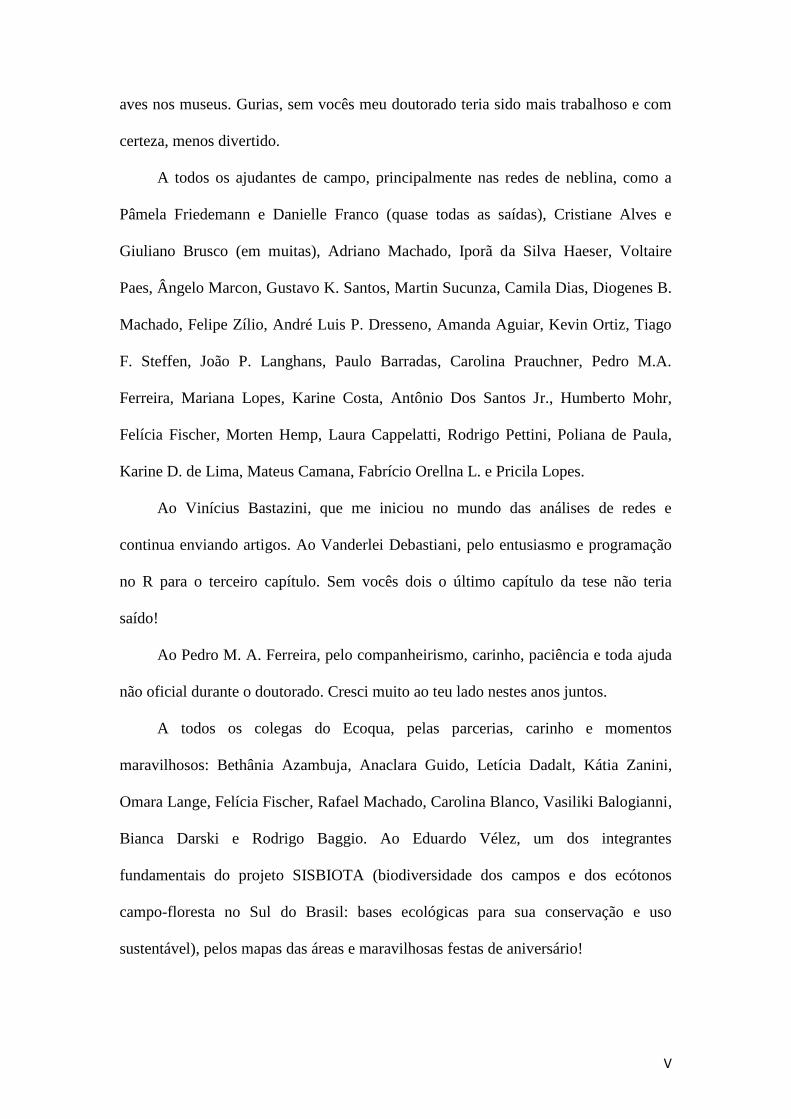
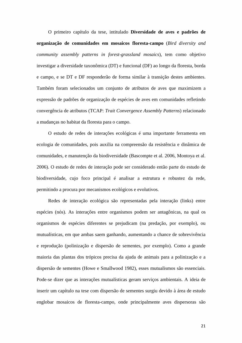
Figure 2. Measures of bird morphological traits. (A) culmen-Cl, (B) beak height-Bh

and width-Bw, (C) wing length-Wl, (D) external-Er and mid rectrix-Mr of tail, (E)

tarsus length-Tl, (F) digit III-Dl, claw of digit III-Cd, hallux-Hl and claw of hallux-

Ch. Adapted from Sick (1997).....................................................................................42

Figure 3. Diversity profiles for forest (FO), edge (ED) and grassland (GR) using the

Rényi entropy index. ...................................................................................................49

Figure 4. Ordination of sampling units described by avifauna species composition

across forest (black symbols), forest edges (gray symbols) and grassland (white

symbols) habitat types, in CCS region (squares), SS region (circles), and CA region

(triangle), represented by the first two ordination axes (PCoA). Species with highest

scores values in the first 2 axis are shown. Species labels: Elme- Elaenia mesoleuca,

Elpa- Elaenia parvirostris, Laeu- Lathrotriccus euleri, Myma- Myiodynastes

maculatus, Myle- Myiothlypis leucoblephara, Pava- Pachyramphus validus, Pisu-

Pitangus sulphuratus, Prta- Progne tapera, Sepi- Setophaga pitiayumi, Thru-

Thamnophilus ruficapillus, Trmu- Troglodytes musculus, Tyme- Tyrannus

melancholicus, Xoir- Xolmis irupero, Zoca- Zonotrichia capensis............................51

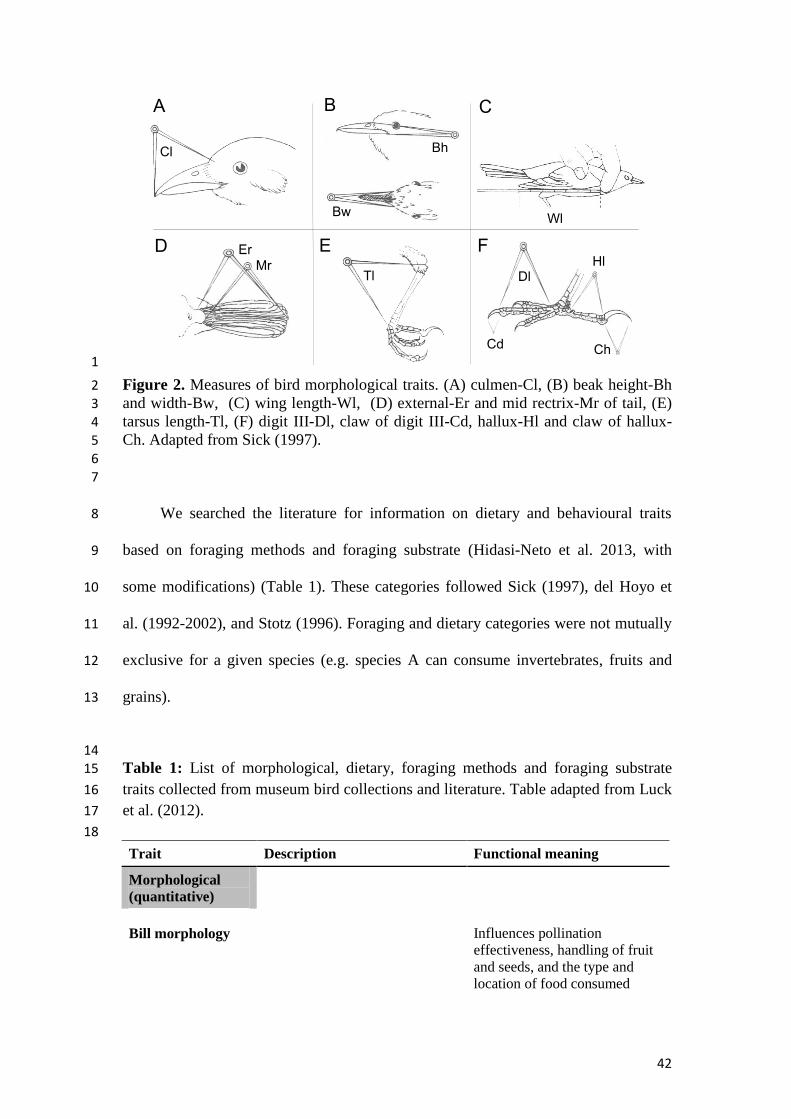
Figure 5. PCoA based on fuzzy-weighted composition of birds on 27 communities

(matrix X) from Southern of Brazil. The community-weighted mean traits (matrix T)

were projected on the diagram based on their correlations with the ordination axes.

Labels for traits: Cldi- claw of digit III, Bcur- beak curvature, Mire- mid rectrix,

Dinv- diet invertebrate, Dgra- diet grans, Bgle- gleaning foraging method, and Fveg-

vegetation foraging substrate. Sampling units are color-coded according to habitat

type: forest (black symbols), forest edge (gray symbols), and grassland (white

symbols). Different symbols indicate different sampling regions: CCS (squares), SS

(circles) and CA (triangle)............................................................................................53

Figure 6. Functional diversity (Rao’s quadratic entropy index) on forest (FO), edge

(ED) and grassland (GR), based on composition of bird species in 27 communities

(matrix W) from Southern of Brazil. Different letters indicate significant differences

between forest, edge and grassland..............................................................................54

14

Appendix Figure 1: Point counts on forest (FO), forest edge (ED) and grassland

(GR) habitats in nine study areas: letter A to C correspond to CCS region; D to F SS;

and G to I CA region....................................................................................................66

Appendix Figure 2: Traits that maximized the correlation between functional

community patterns and the habitat types, in forest (FO), forest edges (ED), and

grassland (GR) habitats. Different letters indicate significant differences between

forest, edges and grassland...........................................................................................72

CAPÍTULO 2

Figure 1. Rio Grande do Sul state with South America and Brazil insert; map of the

dominant vegetation physiognomies of Southern Brazil (IBGE 2004). Numbers

represent the study locations in CCS (1 and 2) and SS (3 and 4) areas.......................78

Figure 2: Cumulative distribution of connectivity (number of links per species, k, or

degree) for 18 seed dispersal interaction networks. Panels show the cumulative

distributions of species with 1, 2, 3, ..., k links (dots), exponential fits (light gray),

power-law fits (gray lines) and truncated power-law fits (black lines). See network

codes in Table 1. We do not show network Ca1 because no model fitted the

distributions of links per species..................................................................................86

Figure 3: Seed dispersal networks sampled in Rio Grande do Sul state, Brazil (Ca1

and Ca2 respectively). Node size is proportional to abundance of species and link

width is proportional to the number of interaction events. Red nodes depict plant

species, whereas yellow nodes are bird species. Bird species lables: Bale- Basileuterus

leucoblepharus, Chca- Chiroxiphia caudata, Cych- Cyanocorax chrysops, Elpa- Elaenia

parvirostris, Elme- Elaenia mesoleuca, Elsp- Elaenia sp., Kncy- Knipolegus cyanirostris,

Myma- Myiodinastes maculatus, Pavi- Pachyramphus viridis, Syru- Syndactyla

rufosuperciliata, Tapr- Tangara preciosa, Tasa- Tangara sayaca, Tual- Turdus albicollis,

Tuam- Turdus amaurochalinus, Turu- Turdus rufiventris, Viol- Vireo olivaceus, Zoca-

Zonotrichia capensis. Plant species lables: Bato- Banara tomentosa, Cist- Cissus striata,

Dara- Daphnopsis racemosa, Dran- Drimys angustifolia, Euun- Eugenia cf. uniflora, Euur-

Eugenia uruguaiensis, Ilsp- Ilex sp., Libr- Lithraea brasiliensis, Masp- Maytenus sp., Misp-

Miconia sp., Mypa- Myrcia palustris, Myat- Myrrhinium atropurpureum, Mysp- Myrsine sp.,

Myrt- Myrtaceae, Posa- Pouteria salicifolia, Scle- Schinus lentiscifolius, Scbu- Scutia

buxifolia, Stle- Stirax leprosus, Trac- Tripodanthus acutifolius, Mo- morph, plant species

where the seeds could not be identified. Image produced with FoodWeb3D, written by

R.J. Williams and provided by the Pacific Ecoinformatics and Computational Ecology

Lab (http://www.foodwebs.org)...................................................................................87

Figure 4: Importance index (I) of the Ca1 network for the bird species as dispersers

and for plant species suppliers of fruit resources for birds. Network sampled in Rio

Grande do Sul state, Campos de Cima da Serra region, Brazil...................................89

15

Figure 5: Importance index (I) of the Ca2 network for the bird species as dispersers

and for plant species suppliers of fruit resources for birds. Network sampled in Rio

Grande do Sul state, Serra do Sudeste region, Brazil. Morph = plant species where the

seeds could not be identified........................................................................................90

CAPÍTULO 3

Figure 1. Observed value (star), median and confidence limits of Connectance,

Nestedness (NODF) and Modularity metrics obtained by resampling with replacement

method using three quantitative mutualistic networks (plants and frugivore birds) and

number of interaction events as sample size. The 95% confidence intervals are set

based on 100 resampling interactions at each sample size. See table 1 for detailed

information of networks.............................................................................................112


Nestedness (NODF) and Modularity metrics obtained by resampling with replacement

method using two quantitative mutualistic networks (plants and frugivore birds) and

number of bird individuals captured as sample size. The 95% confidence intervals are

set based on 100 resampling interactions at each sample size. See table 1 for detailed

information of seed-dispersal networks (bird and plant) Casas 1 and Casas 2.

....................................................................................................................................113

Supplementary material Figure 1: Observed value (star), median and confidence

limits of Connectance, Nestedness (NODF) and Modularity metrics obtained by

resampling with replacement method using Schleuning et al. (2011) mutualistic

network with the data collected only in a secondary forest, and number of interaction

events as sample size. The 95% confidence intervals are set based on 100 resampling

interactions at each sample size..................................................................................121

16

LISTA DE TABELAS

CAPÍTULO 1

Table 1: List of morphological, dietary, foraging methods and foraging substrate

traits collected from museum bird collections and literature. Table adapted from Luck

et al. (2012)..................................................................................................................42

Appendix Table 1. Species registered in the listening points in forest, forest edges

and grassland habitats. Scientific nomenclature is in accordance to the rules

established by the Brazilian committee of ornithological records (Comitê Brasileiro de

Registros Ornitológicos 2014).....................................................................................67

CAPÍTULO 2

Table 1: Description of the 19 plant-frugivore networks. Information about dataset

source, habitat type, location, data type, methodology approach and the number of

species of birds and plants are given............................................................................80

Table 2: Descriptors of the 19 plant-frugivore networks: NODF- nested overlap and

decreasing fill; CON- connectance; MOD- modularity; Pl D. and An D.- plant and

bird degree distributions respectively; K.M Pl and K.M An– Medium Degree of both,

birds and plants.............................................................................................................84

CAPÍTULO 3

Table 1: Description of the three plant-frugivore networks datasets used with the

bootstrap resampling technique..................................................................................109

Supplementary material Table 1: Extension of Figure 01 and 02, in the main text of

the paper, and Supplementary Material Figure 01, with details of observed metric

values, median and confidence intervals obtained by resampling with replacement

method. The values are the 95% confidence intervals (CI) based on 100 resampling

interactions only with the maximum number of interaction events for each seed

dispersal network. ......................................................................................................120

Supplementary material Table 2: Example of a matrix (network Casas 1) with

interactions events and its dismember matrix used to resampling interactions with

replacement according to the bootstrap method. Row represents the code of bird

species and columms the plant species.......................................................................122

17

Supplementary material Table 3: Example of a matrix (network Casas 1) used with

bootstrap method with the bird individuals captured as sample size. Row represents

the code of bird species and columms the plant species............................................123

Supplementary material Table 4: Example of a matrix (network Casas 2) used in

the script bellow (object “SS.txt”) of bootstrap method. Row represents the code of

bird species and columms the plant species...............................................................126

18

INTRODUÇÃO GERAL

Por que espécies são abundantes como são? Por que elas ocorrem neste e não

naquele lugar? Como as comunidades se organizam no tempo e no espaço? Quais os

processos ecológicos que governam a estrutura de comunidades? Tais

questionamentos e a busca por processos ecológicos através dos padrões é o que mais

instiga pesquisadores em ecologia de comunidades, e consequentemente, é o principal

foco da presente tese.

Uma das abordagens teóricas acerca da compreensão destes padrões inclui

padrões de organização de comunidades ou regras de montagem (assembly rules).

Neste contexto, o principal objetivo é predizer qual subconjunto do pool total de

espécies de uma dada região ocorrerá em um habitat específico (Diaz et al. 1999).

Diamond (1975) descreveu como as interações bióticas influenciam a limitação da

composição de espécies em escala local, tanto por exclusão competitiva (Gause 1934)

quanto por limitação de similaridade (MacArthur e Levins 1967). De acordo com a

limitação de similaridade, espécies com uso de recurso e atributos funcionais

semelhantes competirão, e para que coexistam, é preciso haver dissimilaridade entre

estas ou complementaridade.

Condições ambientais agem como filtros, permitindo que somente espécies com

determinadas características ecológicas e fisiológicas se estabeleçam nestes locais

(Zobel 1997). Cada indivíduo, de acordo com a teoria do nicho (Grinnell 1917, Gause

1934), se estabelecerá somente em habitats onde as condições ambientais locais forem

propícias à sua sobrevivência e reprodução. Por outro lado, segundo a teoria neutra

(Hubbell 2001), as comunidades ecológicas são estruturadas por deriva

(estocasticidade demográfica), com todos os indivíduos de uma comunidade

19

possuindo igual probabilidade de reproduzir, morrer ou migrar (Hubbell 2005). No

entanto, uma teoria não exclui a outra, e ambas podem agir na estruturação de

comunidades (Gravel et al. 2006).

A partir da perspectiva de nicho, a organização das comunidades envolve

convergência e divergência de atributos das espécies (Pillar et al. 2009). O padrão de

organização a partir da convergência de atributos (TCAP: Trait Convergence

Assembly Patterns) está relacionado à capacidade das espécies em transpor os filtros

ambientais, e consequentemente, as espécies que coocorrem em uma dada

comunidade tendem a apresentar similaridade na expressão de determinados atributos

(Keddy 1992, Weiher et al. 1998, Pillar e Duarte 2010). Por outro lado, a limitação de

similaridade leva a padrões de organização de divergência de atributos entre espécies

(TDAP: Trait Divergence Assembly Patterns) (Macarthur e Levins 1967, Pillar e

Duarte 2010). Pillar et al. (2009) apresentam um método para discriminar TCAP e

TDAP nas comunidades em relação a gradientes ecológicos, baseado em correlações e

correlações parciais de matrizes descritas por espécies, atributos e variáveis

ambientais. TCAP pode ser identificado quando áreas vizinhas ao longo de um

gradiente ecológico apresentam espécies com similaridade nos atributos, e mudanças

nos mesmos podem estar relacionadas a este gradiente (Pillar et al. 2009).

Avaliações de padrões de organização de comunidades podem ser feitas com

base na composição de espécies (Diamond 1975) ou pelos atributos funcionais das

espécies (Pillar et al. 2009). Atributos funcionais de aves vêm sendo utilizados para

acessar a resposta funcional a diferentes tipos de mudanças ecossistêmicas

(Vandewalle et al. 2010), e para realizar predições sobre mudanças na diversidade

biológica e funcional em resposta às modificações do habitat (Hausner et al. 2003).

Assim, a abordagem de atributos funcionais e diversidade funcional vêm crescendo

20

nos últimos anos com objetivo de responder a questões ecológicas (Mason e de Bello

2013). A diversidade funcional é um parâmetro que leva em consideração as

diferenças funcionais entre as espécies de uma comunidade, ou seja, considera a

variação dos atributos funcionais (Tilman et al. 2007).

Apesar de estudos clássicos com diversidade taxonômica e riqueza de espécies

serem essenciais, eles podem ser insuficientes em capturar as interações ocorrendo no

ecossistema, porque geralmente assumem que todas as espécies são igualmente

distintas em relação a suas influências sobre relações ecológicas (Mouchet et al.

2010). Recentes estudos sugerem que atributos funcionais são mais eficazes em

predizer os efeitos de mudanças globais sobre serviços ecossistêmicos quando

comparado com a diversidade de espécies (Cadotte et al. 2011), e que ambos podem

capturar diferentes processos de organização de comunidades ao longo de gradientes

ecológicos (Bernard-Verdier et al. 2013, Janeček et al. 2013).

Este estudo foi realizado em um gradiente ecológico de mosaicos floresta-

campo no sul do Brasil, facilitando a investigação de padrões de comunidades de aves

e a importância das restrições ambientais impostas por filtros na transição floresta-

campo (na presente tese foi utilizada a categorização dos tipos de habitats como um

gradiente de estrutura do habitat). O Sul do Brasil está situado em uma zona de

transição entre vegetação tropical ao norte e vegetação de clima temperado ao sul

(Overbeck et al. 2007). No Rio Grande do Sul, os ecossistemas campestres formam

zonas de transição (ecótonos) com Florestas Ombrófilas Mistas (floresta com

Araucária) e Estacionais. Os campos sulinos caracterizavam o sul do Brasil bem antes

da expansão das formações florestais, e estudos palinológicos demonstraram que a

formação de mosaicos campo-floresta foi fortemente determinada por alterações

climáticas do Quaternário (Behling and Pillar 2007).

21

O primeiro capítulo da tese, intitulado Diversidade de aves e padrões de

organização de comunidades em mosaicos floresta-campo (Bird diversity and

community assembly patterns in forest-grassland mosaics), tem como objetivo

investigar a diversidade taxonômica (DT) e funcional (DF) ao longo da floresta, borda

e campo, e se DT e DF responderão de forma similar à transição destes ambientes.

Também foram selecionados um conjunto de atributos de aves que maximizem a

expressão de padrões de organização de espécies de aves em comunidades refletindo

convergência de atributos (TCAP: Trait Convergence Assembly Patterns) relacionado

a mudanças no habitat da floresta para o campo.

O estudo de redes de interações ecológicas é uma importante ferramenta em

ecologia de comunidades, pois auxilia na compreensão da resistência e dinâmica de

comunidades, e manutenção da biodiversidade (Bascompte et al. 2006, Montoya et al.

2006). O estudo de redes de interação pode ser considerado então parte do estudo de

biodiversidade, cujo foco principal é analisar a estrutura e robustez da rede,

permitindo a procura por mecanismos ecológicos e evolutivos.

Redes de interação ecológica são representadas pela interação (links) entre

espécies (nós). As interações entre organismos podem ser antagônicas, na qual os

organismos de espécies diferentes se prejudicam (na predação, por exemplo), ou

mutualísticas, em que ambas saem ganhando, aumentando a chance de sobrevivência

e reprodução (polinização e dispersão de sementes, por exemplo). Como a grande

maioria das plantas dos trópicos precisa da ajuda de animais para a polinização e a

dispersão de sementes (Howe e Smallwood 1982), esses mutualismos são essenciais.

Pode-se dizer que as interações mutualísticas geram serviços ambientais. A ideia de

inserir um capítulo na tese com dispersão de sementes surgiu devido à área de estudo

englobar mosaicos de floresta-campo, onde principalmente aves dispersoras são

22

importantes no processo de expansão florestal. Estas aves contribuem na fase inicial

de nucleação de árvores, pois transportam diásporos da floresta para o campo (Duarte

et al. 2006). A primeira pergunta para o surgimento do capítulo dois foi: ‘quem

dispersa o quê’ e ‘quais as espécies de aves e plantas são mais importantes na

dispersão?’. Para responder a estas questões, duas redes de interação ave-planta foram

coletadas em duas regiões diferentes no estado do Rio Grande do Sul.

Como a busca por processos ecológicos através dos padrões é o que mais instiga

pesquisadores em ecologia, outras perguntas então surgiram relacionadas a este

capítulo: qual é a estrutura da rede de interação coletada nestas áreas de mosaicos

floresta-campo? O padrão encontrado nas redes coletadas é o mesmo comparando

outras redes de interação ave-planta coletadas em outros continentes? O que se

encontra na literatura é que processos coevolutivos entre redes mutualísticas e

antagônicas podem divergir, e consequentemente, a estrutura destes tipos de redes

ecológicas serão também diferentes (Lewinsohn et al. 2006). No entanto, para redes

mutualísticas, principalmente comparando interação planta-polinizador e dispersor,

espera-se que tais redes apresentem uma estrutura em comum. Por exemplo, em dois

estudos clássicos comparando redes de polinização e dispersão, Bascompte et al.

(2003) e Jordano et al. (2003), encontraram que redes mutualísticas são geralmente

aninhadas, isto é, espécies especialistas (com poucas interações) interagem com um

subconjunto de espécies que também interagem com as espécies generalistas (espécies

com muitas interações). Redes mutualísticas são geralmente caracterizadas por poucas

espécies supergeneralistas, sendo que a maioria das espécies apresentam poucas

interações.

Algumas redes mutualísticas também são modulares, ou seja, um subgrupo de

espécies (módulos) interagem mais entre si do que com espécies de outros subgrupos.

23

Em redes de interação planta-polinizador, a modularidade aumenta a estabilidade da

rede, pois distúrbios em cascatas parecem se dissipar lentamente em uma rede

modular do que em redes não modulares (Olesen et al. 2007). Estudos prévios

também encontraram modularidade em redes de dispersão de sementes ave-planta

(Mello et al. 2011, Vidal et al. 2014), apesar deste padrão ter sido pouco investigado

em redes de dispersão de sementes. Inclusive, em comparação com números de

estudos realizados com redes mutualísticas, polinização é bem mais estudada

comparado a redes de interação planta-dispersor (Miranda et al. 2013).

O segundo capítulo da tese, intitulado Estrutura de redes de dispersão de

sementes de plantas por aves (Structure of seed-dispersal networks between birds

and plants), teve como objetivo analisar a estrutura de redes de dispersão de sementes

ave- planta, utilizando as métricas de rede: aninhamento, modularidade, conectância

(proporção de links observados na rede de interação relativo aos links possíveis) e

distribuição do grau (probabilidade de encontrar uma espécie com um determinado

número de interações). Além das duas redes coletadas em mosaicos floresta-campo no

estado do Rio Grande do Sul, outras 17 redes foram analisadas para acessar padrões

de redes mutualísticas entre ave e planta, incluindo uma rede de outro pesquisador

também coletada no estado. O índice de importância foi utilizado para verificar quais

foram as aves e as plantas mais importantes das redes, mas somente com aquelas

coletadas nesta tese.

As redes coletadas foram muito pequenas, totalizando 43 espécies de aves e

plantas nos municípios de Santana da Boa Vista e Herval, e apenas 16 espécies em

Jaquirana e Cambará do Sul. Para a menor rede, o aninhamento não foi significativo e

também não foi possível estimar a distribuição do grau. Devido aos resultados desta

segunda rede e ao seu tamanho, iniciou-se uma discussão sobre suficiência amostral

24

em redes de interação. Será que esta rede não é aninhada ou o não aninhamento foi

devido ao tamanho amostral? Além disto, uma questão muito abordada pelo grupo do

laboratório “Ecologia Quantitativa” é: suficiente para quê? A menor rede coletada

pode não ter sido suficiente para a métrica “aninhamento”, mas foi suficiente para

“modularidade”?

Amostrar uma considerável parte da diversidade de interações é um esforço

intenso, e é provável que a maioria dos dados que se tem na literatura não tenham sido

suficientemente amostrados. Chacoff et al. (2012) realizaram uma intensa

amostragem, mas detectaram menos de 60% do potencial de interações. Em relação a

redes de dispersão de sementes, a maioria das redes publicadas são pequenas e,

provavelmente, insuficientemente amostradas. Além do tamanho pequeno da maioria

das redes de interação ave-planta, muitas métricas de rede são sensíveis ao esforço

amostral e ao tamanho da rede (Dormann et al. 2009). Olesen et al. (2007) encontrou

uma relação entre o tamanho de redes planta-polinizador com aninhamento e

modularidade. A conectância apresentou uma correlação negativa com o tamanho da

rede (Mello et al. 2011). Bascompte et al. (2003) encontraram que, para redes planta-

frugívoro e planta-polinizador, acima de 50 espécies, todas as redes de interação

foram significativamente aninhadas. Consequentemente, estudos que apresentam um

baixo esforço amostral precisam ser interpretados com cautela (Rivera-Hutinel et al.

2012).

A teoria estatística objetiva responder três perguntas: a) como os dados devem

ser coletados; b) como devem ser analisados; e c) quão preciso são os dados. A

terceira questão faz parte do processo conhecido como inferência estatística (Efron e

Tibshirani 1993), e foi um dos objetivos do terceiro capítulo da tese, utilizando o

método de reamostragem com reposição bootstrap (Efron 1979, Efron e Tibshirani

25

1993, Pillar 1998). O método bootstrap parte do princípio que a distribuição dos

valores observados em uma amostra é o melhor indicativo da distribuição no universo

amostral em que a amostra foi coletada. A reamostragem no método ocorre com

reposição, imitando a reamostragem do universo amostral.

Tendo em vista a influência do tamanho amostral nas métricas de rede e que a

maioria das redes de interação ave-planta são pequenas, no terceiro capítulo,

intitulado Avaliação de suficiência amostral em métricas de redes de interação

utilizando bootstrap (Assessing sampling sufficiency of network metrics using

bootstrap), o objetivo foi desenvolver um método estatístico visando avaliar

suficiência amostral para algumas das mais utilizadas métricas de redes de interação,

com o método de reamostragem com reposição bootstrap. Foram utilizadas três redes

quantitativas de interação ave-planta (que inclui a frequência da interação) como

exemplo, e as métricas conectância, aninhamento e modularidade.

Área de estudo

Esta tese fez parte do projeto SISBIOTA (Biodiversidade dos campos e dos

ecótonos campo-floresta no Sul do Brasil: bases ecológicas para sua conservação e

uso sustentável). A tese se enquadrou em um dos objetivos da rede de pesquisa do

projeto: a identificação de padrões taxonômicos, funcionais e filogenéticos de

organização de espécies da flora e da fauna em comunidades biológicas características

dos campos sulinos e ecossistemas florestais associados. As áreas de ecótono

(mosaicos floresta-campo) pertencentes ao projeto foram localizadas nos seguintes

municípios: Cambará do Sul, Jaquirana, São Francisco de Paula (região fisiográfica

Campos de Cima da Serra), Encruzilhada, Santana da Boa Vista, Herval (Serra do

Sudeste), Santana do Livramento, Santo Antônio das Missões e São Francisco de

26

Assis (Campanha).

A definição das unidades amostrais foi estabelecida mediante um delineamento

amostral comum para os diferentes grupos biológicos em que foram selecionadas

Unidades Amostrais de Paisagem (UAPs) de tamanho 2x2 km e, dentro destas,

Unidades Amostrais na Escala Local (UALs) com 70x70 m. Para tanto, adotou-se

uma abordagem sistemática e padronizada de escolha das unidades amostrais,

combinando estratificação e aleatorização, a partir do conhecimento espacializado

sobre a distribuição atual e pretérita dos campos e ecótonos no Rio Grande do Sul.

Dentro de cada UAP de ecótono foram estabelecidas cinco UALs (Figura 1).

Três UALs foram estabelecidas sobre área de campo (70x70 m), preferencialmente

sem evidência de colonização por indivíduos lenhosos florestais. As outras duas

UALs foram alocadas em áreas de borda floresta-campo, que apresentavam

evidências de expansão da floresta sobre o campo (Figura 2). Cada UAL de borda

floresta-campo foi composta por duas parcelas contíguas de 70x70 m cada, sendo uma

parcela orientada para o interior da área predominantemente campestre e a outra

parcela orientada para o interior da área florestal (Figura 1).

A amostragem da avifauna para o primeiro capítulo foi realizada em todas as

nove áreas na escala de paisagem (UAP), mas quando possível, no interior ou

próximo das UALs do projeto. Os pontos de escuta para amostragem da avifauna

sempre foram realizados com no mínimo 100 m de distância da borda da floresta, e

consequentemente, fora das UALs florestais. Também foi criada para a tese mais uma

UAL em área de borda floresta-campo. A captura da avifauna para coleta de sementes

no segundo capítulo foi realizada em quatro das nove áreas de ecótono: Jaquirana,

Cambará do Sul (Campos de Cima da Serra), Santana da Boa Vista e Herval (Serra do

Sudeste). As 16 redes de neblina foram alocadas no interior da floresta (fora das

27

UALs florestais) e na borda da floresta. Foram utilizadas oito redes de neblina em

cada ambiente.

Figura 1. Exemplo de demarcação das unidades amostrais em áreas de ecótonos

pertencente ao projeto SISBIOTA. Ao fundo, imagem de satélite do aplicativo Google

Earth. As linhas brancas delimitam a UAP (Unidades Amostral de Paisagem) e as

UALs.

28

Figura 2. Fisionomia da vegetação nas UALs borda floresta-campo e campo do

projeto SISBIOTA no Rio Grande do Sul. A região fisiográfica Campos de Cima

da Serra está representada pelas figuras A a F; Serra do Sudeste de G a I; e

Campanha de J a O.

29

REFERÊNCIAS BIBLIOGRÁFICAS

Bascompte, J., P. Jordano, C. J. Melián, and J. M. Olesen. (2003). The nested

assembly of plant-animal mutualistic networks. Proceedings of the National

Academy of Sciences 100:9383–9387.

Bascompte, J., P. Jordano, and J. M. Olesen. (2006). Asymmetric coevolutionary

networks facilitate biodiversity maintenance. Science 312:431–433.

Behling, H., and V. D. Pillar. (2007). Late Quaternary vegetation, biodiversity and

fire dynamics on the southern Brazilian highland and their implication for

conservation and management of modern Araucaria forest and grassland

ecosystems. Philosophical transactions of the Royal Society of London B,

Biological Sciences 362:243–251.

Bernard-Verdier, M., O. Flores, M.-L. Navas, and E. Garnier. (2013). Partitioning

phylogenetic and functional diversity into alpha and beta components along an

environmental gradient in a Mediterranean rangeland. Journal of Vegetation

Science 24:877–889.

Cadotte, M. W., K. Carscadden, and N. Mirotchnick. (2011). Beyond species:

Functional diversity and the maintenance of ecological processes and services.

Journal of Applied Ecology 48:1079–1087.

Chacoff, N. P., D. P. Vázquez, S. B. Lomáscolo, E. L. Stevani, J. Dorado, and B.

Padrón. (2012). Evaluating sampling completeness in a desert plant-pollinator

network. Journal of Animal Ecology 81:190–200.

Diamond, J. M. (1975). Assembly of species communities. Pages 342–444. In M. L.

Cody and J. M. Diamond, editors. Ecology and evolution of communities.

Harvard University Press, Cambridge, Massachusetts, USA.

Diaz, S., M. Cabido, F. Casanoves, E. Weiher, and P. Keddy. (1999). Functional

implications of trait-environment linkages in plant communities. Pages 338–362.

In Ecological assembly rules: Perspectives, advances, retreats. Cambridge

University Press

Dormann, C. F., J. Frund, N. Bluthgen, and B. Gruber. (2009). Indices, Graphs and

Null Models: Analyzing Bipartite Ecological Networks. The Open Ecology

Journal 2:7–24.

Duarte, L. D. S., M. M. G. Dos-Santos, S. M. Hartz, and V. D. P. Pillar. (2006). Role

of nurse plants in Araucaria Forest expansion over grassland in south Brazil.

Austral Ecology 31:520–528.

Efron, B. (1979). Bootstrap methods: another look at the jackknife. The Annals of

Statistics 7:1–26.

30

Efron, B., and R. J. Tibshirani. (1993). An introduction to the bootstrap. Chapman and

Hall, London, UK.

Gause, G. F. (1934). The struggle for existence. Baltimore, Maryland. Williams and

Wilkins.

Gravel, D., C. D. Canham, M. Beaudet, and C. Messier. (2006). Reconciling niche

and neutrality: the continuum hypothesis. Ecology Letters 9:399–409.

Grinnell, J. (1917). The niche-relationships of the California Thrasher. The Auk

34:427–433.

Hausner, V. H., N. G. Yoccoz, and R. A. Ims. (2003). Selecting indicator traits for

monitoring land use impacts: birds in northern coastal birch forests. Ecological

Applications 13:999–1012.

Howe, H. F., and J. Smallwood. (1982). Ecology of seed dispersal. Annual Review of

Ecology and Systematics 13:201–228.

Hubbell, S. P. (2001). The unified neutral theory of biodiversity and biogeography.

Princeton University Press, Princeton, New Jersey, USA.

Hubbell, S. P. (2005). Neutral theory in community ecology and the hypothesis of

functional equivalence. Functional Ecology 19:166–172.

Janeček, Š., F. Bello, J. Horník, M. Bartoš, T. Černy, J. Doležal, M. Dvorsk\`y, K.

Fajmon, P. Janečková, Š. Jiráská, O. Mudrák, and J. Klimešová. (2013). Effects

of land-use changes on plant functional and taxonomic diversity along a

productivity gradient in wet meadows. Journal of Vegetation Science 24:898–

909.

Jordano, P., J. Bascompte, and J. M. Olesen. (2003). Invariant properties in

coevolutionary networks of plant – animal interactions. Ecology Letters 6:69–81.

Keddy, P. A. (1992). Assembly and response rules: two goals for predictive

community ecology. Journal of Vegetation Science 3:157–164.

Lewinsohn, T. M., Prado, P. I., Jordano, P., Bascompte, J., and Olesen, J. M. (2006).

Structure in plant -animal interaction assemblages. Oikos 113:1–11.

Macarthur, R., and R. Levins. (1967). The Limiting Similarity, Convergence, and

Divergence of Coesxisting Species. The American Naturalist 101:377–385.

Mason, N. W. H., and F. de Bello. (2013). Functional diversity: a tool for answering

challenging ecological questions. Journal of Vegetation Science 24:777–780.

Mello, M. A. R., F. M. D. Marquitti, P. R. Guimarães, E. K. V. Kalko, P. Jordano, and

M. A. M. de Aguiar. (2011). The modularity of seed dispersal: Differences in

31

structure and robustness between bat- and bird-fruit networks. Oecologia

167:131–140.

Miranda, M., F. Parrini, and F. Dalerum. (2013). A categorization of recent network

approaches to analyse trophic interactions. Methods in Ecology and Evolution

4:897–905.

Montoya, J. M., S. L. Pimm, and R. V Solé. (2006). Ecological networks and their

fragility. Nature 442:259–264.

Mouchet, M. a., S. Villéger, N. W. H. Mason, and D. Mouillot. (2010). Functional

diversity measures: An overview of their redundancy and their ability to

discriminate community assembly rules. Functional Ecology 24:867–876.

Olesen, J. M., J. Bascompte, Y. L. Dupont, and P. Jordano. (2007). The modularity of

pollination networks. Proceedings of the National Academy of Sciences of the

United States of America 104:19891–19896.

Overbeck, G. E., S. C. Müller, A. Fidelis, J. Pfadenhauer, V. D. Pillar, C. C. Blanco, I.

I. Boldrini, R. Both, and E. D. Forneck. (2007). Brazil’s neglected biome: The

South Brazilian Campos. Perspectives in Plant Ecology, Evolution and

Systematics 9:101–116.

Pillar, V. D., and L. D. S. Duarte. (2010). A framework for metacommunity analysis

of phylogenetic structure. Ecology Letters 13:587–596.

Pillar, V. D., L. D. S. Duarte, E. E. Sosinski, and F. Joner. (2009). Discriminating

trait-convergence and trait-divergence assembly patterns in ecological

community gradients. Journal of Vegetation Science 20:334–348.

Pillar, V. D. P. (1998). Sampling sufficiency in ecological surveys. Abstracta

Botanica 22:37–48.

Rivera-Hutinel, A., R. O. Bustamante, V. H. Marin, and R. Medel. (2012). Effects of

sampling completeness on the structure of plant – pollinator networks. Ecology

93:1593–1603.

Tilman, D., J. Knops, D. Wedin, P. Reich, M. Ritchie, and E. Siemann. (2007). The

Influence of functional diversity and composition on ecosystem processes

277:1300–1302.

Vandewalle, M., F. de Bello, M. P. Berg, T. Bolger, S. Dolédec, F. Dubs, C. K. Feld,

R. Harrington, P. A. Harrison, S. Lavorel, P. M. da Silva, M. Moretti, J. Niemelä,

P. Santos, T. Sattler, J. P. Sousa, M. T. Sykes, A. J. Vanbergen, and B. a.

Woodcock. (2010). Functional traits as indicators of biodiversity response to

land use changes across ecosystems and organisms. Biodiversity and

Conservation 19:2921–2947.

32

Vidal, M. M., E. Hasui, M. A. Pizo, J. Y. Tamashiro, W. R. Silva, and P. R.

Guimarães Jr. (2014). Frugivores at higher risk of extinction are the key elements

of a mutualistic network. Ecology 95:3440-3447.

Weiher, E., P. Clarke, and P. a. Keddy. (1998). Community assembly rules,

morphological dispersion, of plant species the coexistence. Oikos 81:309–322.

Zobel, M. (1997). The relative role of species pools in determining plant species

richness: An alternative explanation of species coexistence? Trends in Ecology

and Evolution 12:266–269.

33

CHAPTER 1

BIRD DIVERSITY AND COMMUNITY ASSEMBLY PATTERNS IN FOREST-

GRASSLAND MOSAICS

Artist: Willian Kentridge

This article will be submitted to the journal PLoS One

34

Bird diversity and community assembly patterns in forest-grassland mosaics

Grasiela Casas1,* and Valério D. Pillar1.

1 Graduate Program in Ecology, Universidade Federal do Rio Grande do Sul, Porto

Alegre, Rio Grande do Sul, Brazil.

*Corresponding author: [email protected]

Abstract: Classic studies on taxonomic diversity, although they are essential, do not

consider the functional differences between species in a community. Studies using

functional traits and functional diversity are filling this gap. Our aim was to

investigate how bird taxonomic diversity (TD) and functional diversity (FD) vary

across forest-grassland ecotones. We selected sets of traits (through an iterative

algorithm) that maximize the expression of patterns of trait convergence related to

environments variable of habitat types. For the quantitative survey of the avifauna, we

used the point count method in nine areas located in Southern Brazil. We used

morphological, dietary, foraging substrate and behavioural traits. Bird composition

was different between forest, forest edge and grassland. Regarding TD, only forest

and edges differed. FD was significantly different between grassland and forest, and

between grassland and edges. The similar FD between forest and edges was

influenced by the small differences in vegetation structure, which are much more

evident in comparison with grasslands. Grassland encompassed the highest FD in

comparison with forest and edges, as well as the highest number of exclusive species.

Among all traits, seven maximized the correlation between functional community

patterns and the habitat types: beak curvature, claw of digit three, mid rectrix, diet

grains and invertebrate, gleaning foraging method and vegetation foraging substrate.

The TD and FD responded differently to environmental change from forest to

grassland, and our use of both taxonomic and a functional diversity approaches was

useful to conclude that these two facets of diversity may capture different processes of

community assembly along such transitions. Trait-convergence assembly patterns

indicated niche mechanisms underlying assembly of bird communities, and

differences in environmental variables across forest-edge-grassland habitats are acting

as ecological filters.

Key words: avifauna, ecological filters, ecotone, functional traits, species

composition.

35

Introduction 1

2

Many studies are emerging using functional traits and functional diversity to 3

assess ecological questions (Mason and de Bello 2013). Although classic studies on 4

taxonomic diversity are essential, they may be insufficient to capture the interactions 5

occurring in ecosystems, because they usually assume that species are equally distinct 6

regarding their relative influences and responses to ecological relationships (Mouchet 7

et al. 2010). Functional diversity can be defined as the value and range of the 8

functional differences (i.e. trait differences) among species in a community (Tilman 9

et al. 2007). Recent syntheses and empirical studies have highlighted that functional 10

traits predict the effects of global changes on ecosystem services better than species 11

diversity does (Cadotte et al. 2011). However, some studies showed that the different 12

facets of diversity are not necessarily equivalent and may capture different processes 13

of community assembly along gradients (Bernard-Verdier et al. 2013, Janeček et al. 14

2013). Bird traits have been used to assess the functional response to different kinds 15

of ecosystem change (Vandewalle et al. 2010), and as basis for making predictions 16

about changes in biological and functional diversity in response to land use changes 17

(Hausner et al. 2003). 18

Functional traits can be grouped into two broad categories (not mutually 19

exclusive): 1) traits that influence a species response to the environment and/or 2) 20

traits that exert effects on ecosystem processes (Lavorel and Garnier 2002). Birds 21

exhibit a diverse range of ecological functions, mainly related to what they eat and 22

how/where they look for food (Sekercioglu 2006). Characteristics such as foraging 23

behaviour or diet are crucial to understanding how an animal may respond to 24

environmental changes and how it impacts ecosystem function (Luck et al. 2013). For 25

36

example, in frugivorous birds, the capacity to move between spatially discrete habitat 1

patches can determine, on one hand, a species response to declining landscape 2

connectivity and, on the other, its contribution to forest maintenance through seed 3

dispersal (Luck et al. 2012). Morphological traits can be related to ecological traits 4

(Fitzpatrick 1980), and an indicative of species functions in communities. Most 5

morphological traits are considered as effect traits (Luck et al. 2012). For example, in 6

frugivorous birds bill morphology influences the kinds of seeds a species can eat. On 7

the other hand, some morphological traits can be considered both effect and response 8

traits (e.g. body mass, as an effect trait, will impact on the amount and type of food 9

consumed; as a response traits, large-bodied species are more vulnerable to habitat 10

loss in forests). The classification in responses or effect traits will vary according to 11

the selected environmental change or ecosystem service selected. For instance, a trait 12

may be considered a response trait when it changes across an environmental gradient 13

such as from forest to grassland in ecotones. Previous studies evaluated plants 14

(Müller et al. 2007, Carlucci et al. 2012, Brownstein et al. 2013) and mammals (Luza 15

et al. 2015) with a functional approach in ecotones but, to our knowledge, studies 16

using functional diversity of birds in ecotones are scarce. 17

Niche theory is based on the responses of organisms to environmental 18

conditions and biotic interactions (Weiher and Keddy 1999). In relation to 19

environmental conditions, community assembly involves environmental filters, which 20

lead to a pattern of trait convergence: species colonizing a site with a particular set of 21

environmental conditions will tend to exhibit similarity for certain traits (Keddy 22

1992, Weiher et al. 1998). Trait convergence may be identified when neighboring 23

sites along an ecological gradient consistently contain species with similar traits and 24

changes in these traits are related to the gradient (Pillar et al. 2009). 25

37

Our study was conducted in areas characterized by a natural ecological gradient 1

(mosaics of grassland and different forest formations), enabling us to assess patterns 2

reflecting community assembly processes and the importance of environmental 3

restrictions imposed by ecological filters. The Southern part of Brazil is situated at a 4

transitional zone between tropical vegetation types to the north, and temperate 5

vegetation to the South (Overbeck et al. 2007). Paleopalynological studies have 6

shown that the formation of grassland-forest mosaic in Southern Brazil was strongly 7

influenced by climatic changes during the Quaternary (Behling and Pillar 2007). 8

Here we investigate in forest-grassland mosaics in Southern Brazil how bird 9

taxonomic diversity and functional diversity vary across the transition between forest 10

and grassland and whether or not functional diversity and taxonomic diversity 11

respond similarly to habitat transition from forest to grassland. We searched for sets 12

of traits that maximized the expression of patterns of trait convergence related to 13

environment changes from forest to grassland. We focused on morphological, dietary, 14

foraging behavioural and foraging substrate traits of birds. We hypothesized that 1) 15

forest and forest edge directly in contact with grassland (henceforth edge) have 16

similar species composition and taxonomic diversity due to similarity in vegetation 17

structure compared to grassland; 2) functional diversity is higher in grassland than 18

forest and edges, because of natural environmental heterogeneity; 3) environment 19

changes from forest to grassland act as habitat filtering, leading to trait convergence. 20

21

Methods 22

Study area 23

We conducted the study in nine areas with forest-grassland mosaics in three 24

physiographic regions in the state of Rio Grande do Sul: Campos de Cima da Serra 25

38

(CCS), Campanha (CA) and Serra do Sudeste (SS) (Figure 1). These regions are 1

included in the Atlantic Forest (CCS) and the Pampa (CA, SS) biomes and both are 2

characterized by mosaics of forest and grassland. In the Pampa biome, grasslands 3

cover large continuous areas and forests are mostly restricted to riparian zones, 4

whereas in the Atlantic Forest grasslands are located in the highlands of the South-5

Brazilian Plateau. The Atlantic Forest biome includes tropical rainforest (Atlantic 6

forest sensu stricto), mixed ombrophilous forest (Araucaria forest), and seasonal 7

forests (both deciduous and semideciduous) (Oliveira-Filho and Fontes 2000). 8

The South Brazilian grasslands (known as Campos Sulinos) form a natural 9

ecosystem that has characterized this region long before the forest expansion that 10

took place after mid Holocene (Behling and Pillar 2007, Dümig et al. 2008, Behling 11

et al. 2009). Fire and grazing by domestic animals are considered to be the principal 12

factors impeding expansion of forest over grassland vegetation in the past centuries 13

and under current climatic conditions (Pillar and Quadros 1997). Domestic herbivores 14

were present in our sampling areas, and had access to forest patches. In the CCS 15

areas, cattle grazing is less intense, as sampling was conducted in two conservation 16

units, the Tainhas State Park and the Aparados da Serra National Park. In one of the 17

areas in CCS cattle has been excluded since 1994. 18

19

39

1

Figure 1. Bottom left: South America, Brazil and Rio Grande do Sul state; map of 2

the dominant vegetation physiognomies of Southern Brazil (according to IBGE, 3

2004). Numbers are the study areas location in CCS region (1 to 3), SS region (4 to 6) 4

and CA region (7 to 9), and represent the order of temporal sequence of bird 5

sampling. 6

7

Bird sampling 8

For the quantitative survey of the avifauna, we used the point count method 9

(Bibby et al. 1992). We performed point counts in forest interiors, forest edges and 10

grasslands, with three point counts in each environment, nine per area (Appendix 11

Figure 1). Forest point counts were located between 140 to 240 m from the edge. We 12

performed the point counts located in grassland with minimum distance from edge 13

point of 375 m. A total of 81 point counts were surveyed from December 2011 to 14

January 2012, covering the breeding season that is a favourable time for bird 15

sampling. All individuals seen and/or heard were counted, except those that only flew 16

over the area and, consequently, not using the local habitat. Surveys started 15 min 17

after dawn and lasted 3 h. Permanence in each point was 15 min. The order in which 18

point counts were surveyed varied systematically to avoid bias related to time of day. 19

40

The fixed radius of point counts differed between environments due to 1

influence of vegetation structure on the probability of bird detection (Emlen 1971, 2

Rodgers 1981). Point counts in forest and at edges had 25 m fixed radius and 3

grassland 100 m radius. Birds are less easily detected with increasing distance from 4

observers, mainly in forests, because of concealment by vegetation and increased 5

sound attenuation due to obstruction (Waide and Narins 1988). Therefore, fixed-6

radius circular plots of ≤50 m radius were appropriate for sampling in forest and edge 7

environments. In grassland with low woody densities, on the other hand, the detection 8

of most bird individuals occurs outside 25 m radius, probably due to disturbance 9

created by the observer's presence. For the analyses, we first summed the number of 10

recorded birds obtained in the three point counts in each environment per area, 11

resulting in three sampling units in each area: forest, edge and grassland (Appendix 12

Figure 1). After that, we used the relative number of detection counts of a species 13

standardized by the total number of detected birds in a sampling unit, in order to 14

control the effect of sampling detection differences. The resulting values for each 15

species represented a relative frequency value, which provided information about 16

how much that species is using the local resources. 17

One of our aims is to investigate how bird species traits vary across 18

environmental habitats in transitional areas, from forest to grassland. Since our study 19

area is inserted in a regional context of forest expansion over grasslands, we selected, 20

based on the literature, traits related to habitat use that should be responsive to 21

differences in habitat areas across different environments. Examples of the selected 22

traits and the corresponding process involved are: a) morphological traits related to 23

seed dispersion and pollination, such as bill morphology and b) wing length, which is 24

related to capacity to use open spaces or to manoeuvre through tree canopies, which 25

41

in turn influences resource use, seed dispersal and migratory status. We also used 1

dietary and behavioural data based on foraging methods and foraging substrate. All 2

these traits are related to resource acquisition and are expected to strongly influence 3

biodiversity–ecosystem function relationships. For details on all sampled traits see 4

Table 1. 5

We collected fourteen morphological traits from measurements made on 6

specimens of bird collections of the PUCRS Science and Technology Museum 7

(Museu de Ciências e Tecnologia da PUCRS, Porto Alegre) and the Zoobotanical 8

Foundation of Rio Grande do Sul Museum (Fundação Zoobotânica do Rio Grande do 9

Sul, Porto Alegre) (Figure 2). Subsequently, we also included calculated traits: an 10

index of beak curvature using the ratio between culmen arc and culmen, and an index 11

of beak shape using the ratio between beak height and width (Table 1). For each bird 12

species, we measured one to ten specimens, according to quantity and quality of 13

specimens available at museums. For all analysis we considered the average of 14

measured individuals. To identify redundant morphological measurements, we 15

performed a Pearson correlation test between traits and excluded those that were 16

highly correlated (correlation > 0.80). Six traits were highly correlated: culmen vs. 17

arc of culmen (0.99); claw of digit III vs. arc of its claw (0.81); halux vs. claw of 18

halux (0.85). Thus, culmen, claw of halux and claw arc of digit III were excluded. To 19

exclude the influence of differences on bird body sizes on morphological traits, we 20

divided each trait value by the cubic root of the body mass, in our case, species mean 21

body mass. Although all morphological traits are dependent on body mass, the latter 22

was included as a trait in our analyses due its relationship with various ecosystem 23

functions (see Table 1). 24

42

1

Figure 2. Measures of bird morphological traits. (A) culmen-Cl, (B) beak height-Bh 2 and width-Bw, (C) wing length-Wl, (D) external-Er and mid rectrix-Mr of tail, (E) 3 tarsus length-Tl, (F) digit III-Dl, claw of digit III-Cd, hallux-Hl and claw of hallux-4 Ch. Adapted from Sick (1997). 5

6 7

We searched the literature for information on dietary and behavioural traits 8

based on foraging methods and foraging substrate (Hidasi-Neto et al. 2013, with 9

some modifications) (Table 1). These categories followed Sick (1997), del Hoyo et 10

al. (1992-2002), and Stotz (1996). Foraging and dietary categories were not mutually 11

exclusive for a given species (e.g. species A can consume invertebrates, fruits and 12

grains). 13

14 Table 1: List of morphological, dietary, foraging methods and foraging substrate 15

traits collected from museum bird collections and literature. Table adapted from Luck 16

et al. (2012). 17

18

Trait Description Functional meaning

Morphological

(quantitative)

Bill morphology Influences pollination

effectiveness, handling of fruit

and seeds, and the type and

location of food consumed

43


Exposed culmen

(mm)

Bill tip from the point where the

tips of the forehead feathers

begin to hide the culmen

Culmen arc (mm) Length considering the

curvature, measured with thread

Ratio between

culmen arc and

culmen

Indicative of beak curvature

Beak height

Beak width

Ratio between beak

height and width

Indicative of beak shape Relates to diet and food

handling. One of the

morphological traits that best

predicted foraging behavior of

Tyrant-flycatchers (Botero-

Delgadillo and Bayly 2012).

Wing length (mm) Flight capacity

Tarsus length

(mm)

Can influence foraging

behaviour and hence services

such as pest regulation and

nutrient cycling

Feet morphology

(mm)

Can influence foraging

behaviour and small-scale

nutrient cycling (e.g. scraping

the ground to turnover soil)

Digit III

Claw of digit III

Arc of claw of digit

III

length considering the curvature,

measured with thread

Halux

Claw of halux Indicator of foraging substrate

(Feduccia 1993)

Tail (mm) Can influence foraging

behaviour and foraging

substrate (Botero-Delgadillo

and Bayly 2012)

External rectrix

Mid rectrix

44


Mass (g) the live bird weight Strongly relates to a range of

other traits in birds including

metabolic rate, foraging

behaviour and home-range size

Dietary traits

(presence/absence)

Vertebrates

Invertebrates

Plant vegetative

parts

encompass birds that feed

leaves, and/or flower, young

shoots, roots, bulbs and buds

Fruits

Grains

Nectar

Behavioural

traits based on

foraging methods

(presence/absenc

e)

Impacts all aspects of resource

use by birds. Species with

particular foraging behaviour

traits may be sensitive to

particular environmental

changes.

Pursuit The term usually refers to a

technique of sallying out from a

perch to attack a food item

Gleaning To pick food items from a

nearby substrate, including the

ground, that can be reached

without full extension of legs or

neck (Remsen Jr and Robinson

1990)

Pouncing Bird drops to ground and takes

prey

Grazing

Pecking To drive the bill against the

substrate to remove some of the

exterior of the substrate (Remsen

Jr and Robinson 1990)

Scavenging Scavenging is a carnivorous

feeding behaviour in which the

scavenger feeds on dead animal

45


Probing To insert the bill into cracks or

holes to capture hidden food

(Remsen Jr and Robinson 1990)

(e.g. woodpeckers probe trees

and hummingbirds probe

flowers)

Foraging substrate

(presence/absence)

Dictates where birds will

conduct their foraging activities

Water

Mud

Ground

Vegetation

Air

1 2 Data analysis 3

In our analyses we searched for differences in bird taxonomic and functional 4

diversity between forest-edge-grassland environments, considering species 5

composition, their relative number of recorded species (relative species frequency), 6

and trait values. Due to the larger sampling area on grassland compared to forest and 7

edges, we used Chao 1 (Chao 1984, Colwell and Coddington 1994) to estimate 8

species richness. This estimator uses the number of registered species in a sample, as 9

well as singletons and doubletons, as in the equation below: 10

S1 = Sobs + a2/2b, 11

where Sobs is the number of species in the sample, a is the number of singletons (i.e., 12

the number of species with only a single occurrence in the sample) and b is the 13

number of doubletons (the number of species with two occurrences in the sample). 14

Then, we tested for differences in species richness between environmental 15

types considering both observed (number of species registered) and estimated species 16

richness (Chao 1) using ANOVA with permutation (Manly 2007). We restricted all 17

permutations within regions, because our aim was not to test differences between 18

46

regions, but to compare habitat types. Taxonomic diversity (TD) was estimated using 1

Simpson index, and we used ANOVA with permutation to evaluate differences in TD 2

between forest-edge-grassland habitats, also restricting permutations within regions. 3

We also compared species taxonomic diversity patterns between environments using 4

diversity profile based on Rényi entropy values (Rényi 1961). The different values 5

obtained for Rényi’s entropy series correspond to different diversity indexes, 6

according to the value of the scale parameter α (Melo 2008). As the value of 7

parameter α rises, more weight is given to dominant species over rare ones. 8

Differences in species composition among habitat types were tested through 9

multivariate analysis of variance (MANOVA), using Euclidean distance and with 10

randomization (1000 permutations) following the method described by Pillar and 11

Orloci (1996). Species composition pattern across sampling units (habitat types in 12

each site) was also examined through ordination by principal coordinate analysis 13

(PCoA) (Podani 2000). We used Euclidean distance as the measure of similarity 14

between sampling units. 15

We adopted the method described in Pillar et al. (2009), Pillar and Duarte 16

(2010) for analysing functional patterns and their correlation to environmental 17

gradient, and to select trait subsets maximizing such correlation. For this, we 18

organized the data in three matrices: 1) the relative species frequency in the 19

communities in matrix W of species by sampling units; 2) functional traits describing 20

the bird species in matrix B of species by traits; and 3) the ecological gradient of 21

interest, in our case the ordinal environmental variable of habitat types (3: forest, 2: 22

edge, and 1: grassland) in matrix E, as a gradient of habitat structure. Community-23

weighted mean (CWM) traits were computed by matrix multiplication T = B’W. 24

Matrix T contains the mean of each trait in each community. Then, species pairwise 25

47

similarities based on traits in B were used to define matrix U with degrees of 1

belonging of species to fuzzy sets (Pillar and Orlóci 1991). In matrix U each species 2

(given by the column in U) may simultaneously belong, in functionally terms, to 3

more than one species fuzzy type (the rows of U) based on the species trait 4

similarities, with certain degrees of belonging. In other words, a species a in matrix U 5

could “belong” to species b with, say, a 0.5 degree of belonging, according to the 6

functional similarities between a and b. Values in matrix U range from 0 to 1, and the 7

sum of each column is standardized to 1. By matrix multiplication, X = UW will 8

contain the species composition of the communities after the fuzzy weighting by their 9

trait similarities. Matrix X retains more trait information at the community level than 10

community-weighted means do (Pillar et al. 2013), because it keeps the identity of 11

species (weighted by their trait similarities) and can express the variation 12

(divergence) of its traits between communities too. 13

Our interest was to examine the distribution of traits across the forest-edge-14

grassland environments to possibly identify community assembly processes related to 15

environmental filtering. By using matrix correlation (Mantel), we evaluate the 16

correlation between community distances based on matrices T (trait means) and E 17

(ecological gradient). A strong correlation ρ(TE) indicates the factors directly or 18

indirectly represented in E are involved in ecological filtering of species that, at least 19

for the traits considered in the analysis, consistently produce trait-convergence 20

assembly patterns (TCAP) along the gradient (Pillar et al. 2009, Pillar and Duarte 21

2010). Optimal trait subsets were searched that maximized the correlation ρ(TE) 22

using an algorithm analogous to Pillar and Sosinski Jr. (2003). The significance of the 23

correlation ρ(TE) was tested against a null model. The selected trait subset was used 24

in all following analyses. Matrix X was submitted to ordination by principal 25

48

coordinates analysis (PCoA) using Euclidean distances between sampling units. 1

Matrix T was projected on the ordination diagram based on the correlations between 2

community-weighted mean traits and the ordination axes. With the selected trait 3

subset, we used ANOVA with permutation to evaluate differences in each 4

community-weighted mean trait (matrix T) between forest, edge and grassland 5

habitats. 6

Functional diversity (FD) was estimated using Rao’s quadratic entropy index 7

(Rao 1982), which was computed using the relative species frequency in the 8

communities (matrix W) and the species dissimilarities based on optimal traits. The 9

FD calculated with Rao’s index generalizes Simpson’s index of species diversity 10

because if all species have completely different traits, FD values will be equivalent to 11

Simpson diversity (Pavoine et al. 2004, Ricotta 2005). We used ANOVA with 12

permutation to evaluate differences in FD between forest, edge and grassland 13

habitats. 14

We used software SYNCSA (v 2.9.0) for functional analyses and MULTIV (v 15

3.1.7. beta) for all other analyses, both available at http://ecoqua.ecologia.ufrgs.br. 16

17

Results 18

19

We recorded 137 bird species, distributed in 40 families (Appendix Table 1). 20

Tyrannidae was the most representative family in species richness, and Elaenia 21

mesoleuca and E. parvirostris, both belonging to this family, were the most 22

commonly recorded species. From all species, only 21 occurred across the three 23

environments in the forest-edge-grassland, and the grassland encompassed the higher 24

number of exclusive species (49; 19 in forest and 13 in edge). 25

49

Species richness did not differ significantly (restricting permutations within 1

regions) between forest, edge and grassland using observed or estimated species 2

richness (P=0.10 and 0.72, respectively). Therefore, any differences that might have 3

resulted from comparing data obtained by different sampling radius were minimal 4

and did not affect species richness or diversity estimations. Considering the Rényi 5

entropy index, grasslands showed higher species richness (Figure 3; parameter α at 6

zero), and forest and edge showed similar values. With increasing value of parameter 7

α, forest areas were less influenced by dominance, since the curve remained more 8

constant in comparison with edge and grassland areas. Considering richness alone 9

(parameter a=0), Shannon’s or Simpson’s index (parameter α=1 and 2, respectively), 10

the results would be different due to the influence of dominant species in the edge 11

and grassland. However, when we compared areas using Simpson’s index, there were 12

significant differences in TD between forest and edge (P=0.01), but not between 13

forest and grassland (P=0.27) and between edge and grassland (P=0.35). 14

15

16

Figure 3. Diversity profiles for forest (FO), edge (ED) and grassland (GR) using the 17

Rényi entropy index. 18

19

FO

ED

GR

Div

ers

ity

1.5

2.0

2.5

3.0

Renyi entropy value

0 1 2 3 4 5

50

Multivariate analysis of variance (MANOVA) revealed significant differences 1

in species composition between forest, grassland and edge (P=0.001 between forest 2

and edge; P=0.002 for both, forest and edge compared to grassland). PCoA 3

ordination (Figure 4) showed evidence of segregation between grasslands and the 4

other habitats along axis 2. Besides the significant differences revealed by 5

MANOVA, on the ordination scatter diagram some edge sampling units showed 6

intermediate composition in comparison to forest and grassland. Since the SS region 7

is characterized by a more pronounced mosaic than CCS region, we expected that 8

forest and edge would be more similar regarding species composition, but its edge 9

sampling units were different from forest sampling in species composition. We 10

projected on the ordination diagram the bird species with the highest scores for the 11

first 2 axes, and some species were more associated with grassland, as Xolmis irupero 12

(species dependent of grassland), Thamnophilus ruficapillus, Zonotrichia capensis, 13

Tyrannus melancholicus and Pitangus sulphuratus. The last three species were also 14

recorded in edge environments, but they were more common in grasslands, foraging 15

in trees and shrubs. The same was observed for Elaenia mesoleuca and E. 16

parvirostris, two species recorded in all habitat types, but mostly associated with 17

forest and edge, respectively, on the scatter diagram. 18

19

51

1

Figure 4. Ordination of sampling units described by avifauna species composition 2

across forest (black symbols), forest edges (gray symbols) and grassland (white 3

symbols) habitat types, in CCS region (squares), SS region (circles), and CA region 4

(triangle), represented by the first two ordination axes (PCoA). Species with highest 5

scores values in the first 2 axis are shown. Species labels: Elme- Elaenia mesoleuca, 6

Elpa- Elaenia parvirostris, Laeu- Lathrotriccus euleri, Myma- Myiodynastes 7

maculatus, Myle- Myiothlypis leucoblephara, Pava- Pachyramphus validus, Pisu- 8

Pitangus sulphuratus, Prta- Progne tapera, Sepi- Setophaga pitiayumi, Thru- 9

Thamnophilus ruficapillus, Trmu- Troglodytes musculus, Tyme- Tyrannus 10

melancholicus, Xoir- Xolmis irupero, Zoca- Zonotrichia capensis. 11

12

13

Among all traits, seven maximized TCAP related to the environmental gradient 14

(ordinal environmental variable of habitat types) from forest to grassland 15

(ρ(TE)=0.52; P=0.002): beak curvature, claw of digit three, mid rectrix, diet grains 16

and invertebrate, gleaning foraging method and vegetation foraging substrate. The 17

ordination diagram in Figure 5 is based on bird composition of communities after 18

fuzzy weighting by their trait similarities (matrix X), with CWM traits (matrix T) 19

projected on the diagram based on their correlations with the ordination axes. The 20

diagram showed segregation between forest/edge and grassland sampling units along 21

52

the first axis. On the second axis, there is a gradient from forest to edge and a 1

differentiation in relation to trait mean values: sampling units at the lower right side 2

of the scatter diagram showed birds with higher mean values of beak curvature, and 3

at the upper right side birds with higher mean values of mid rectrix and a higher 4

proportion of gleaning foraging methods. Birds that have grains in their diet were 5

more associated with grassland. We highlight that all morphological traits were 6

standardized by the body mass (divided each trait value by the cubic root of the body 7

mass), and when we refer to higher means in trait values they are proportionately 8

higher according to the species mean body mass. 9

We found significant differences in CWM traits for beak curvature between 10

forest, edge and grassland habitats (P=0.03 between forest and edge; P<0.005 both 11

forest and grassland and between edge and grassland) (Appendix Figure 2). The traits 12

mid rectrix, diet grains, gleaning foraging method and vegetation foraging substrate 13

presented significant differences between forest and edge compared to grassland 14

(P>0.1 between forest and edge; P<0.005 for both between forest and grassland and 15

between edge and grassland). The traits diet invertebrate and claw of digit three did 16

not differ significantly among habitats types (P>0.05). 17

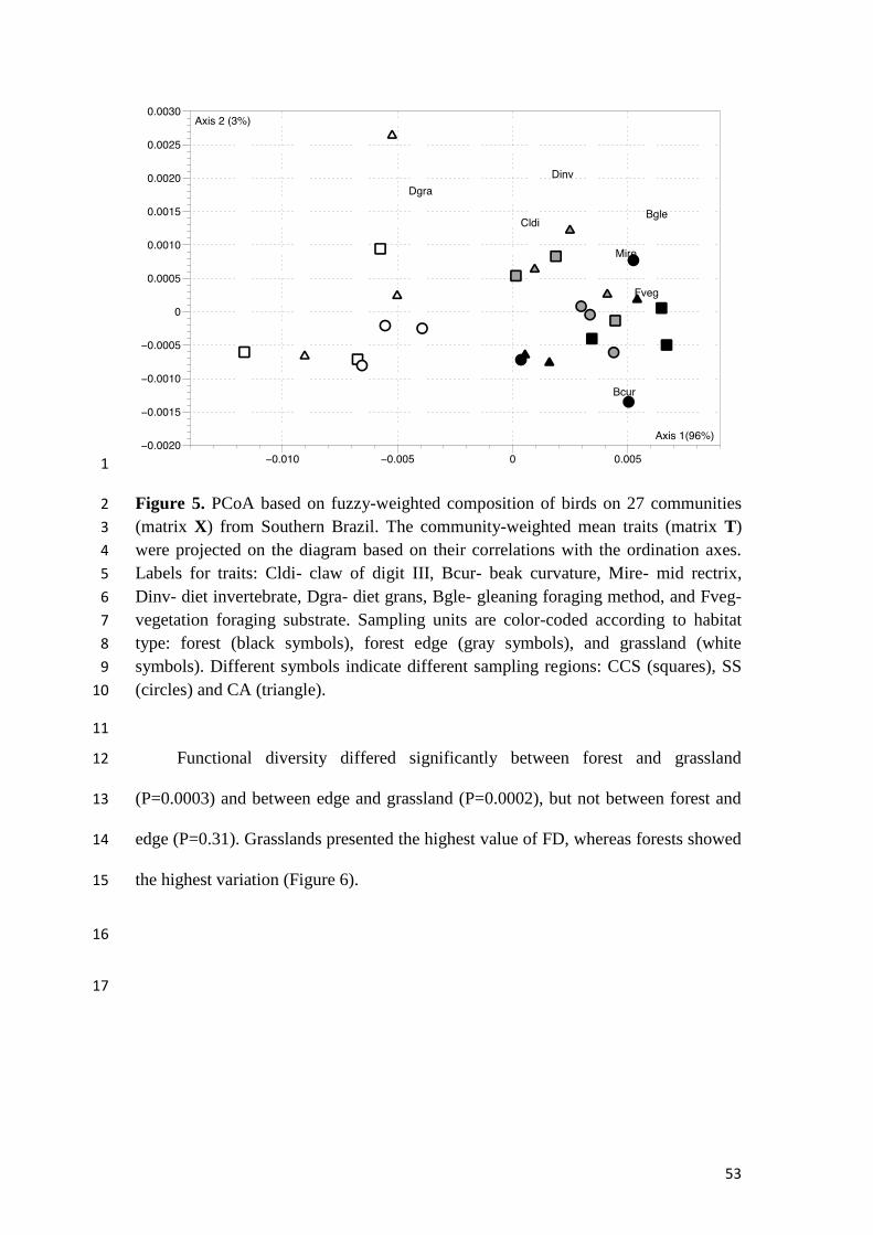
53

1

Figure 5. PCoA based on fuzzy-weighted composition of birds on 27 communities 2

(matrix X) from Southern Brazil. The community-weighted mean traits (matrix T) 3

were projected on the diagram based on their correlations with the ordination axes. 4

Labels for traits: Cldi- claw of digit III, Bcur- beak curvature, Mire- mid rectrix, 5

Dinv- diet invertebrate, Dgra- diet grans, Bgle- gleaning foraging method, and Fveg- 6

vegetation foraging substrate. Sampling units are color-coded according to habitat 7

type: forest (black symbols), forest edge (gray symbols), and grassland (white 8

symbols). Different symbols indicate different sampling regions: CCS (squares), SS 9

(circles) and CA (triangle). 10

11

Functional diversity differed significantly between forest and grassland 12

(P=0.0003) and between edge and grassland (P=0.0002), but not between forest and 13

edge (P=0.31). Grasslands presented the highest value of FD, whereas forests showed 14

the highest variation (Figure 6). 15

16

17

54

1

Figure 6. Functional diversity (Rao’s quadratic entropy index) on forest (FO), edge 2

(ED) and grassland (GR), based on composition of bird species in 27 communities 3

(matrix W) from Southern Brazil. Different letters indicate significant differences 4

between forest, edge and grassland. 5

6

7

Discussion 8

9

We reported differences on species composition, different response between 10

taxonomic and functional diversity across the environments, and a trait convergence 11

related to ordinal environmental variable of habitat types as environmental filters. 12

Bird composition differed between forest-edge-grassland in our study. Baker et 13

al. (2007) found species composition at forest edges in grassland/forest ecotones to be 14

intermediate between the two adjacent communities. In our case, some edge sampling 15

units seemed to have intermediate composition between forest and grassland (Figure 16

4). We recorded 13 species only in the edge environment, including Lanio cucullatus, 17

Nemosia pileata, Polioptila dumicola, Serpophaga subcristata and Synallaxis 18

frontalis, species that usually occur in forest edges. Among the 19 species recorded 19

only in forest, few are characteristic of forest interiors, such as Lanio melanops, 20

b

aa

Fu

nction

al d

ive

rsity (

Rao

)

0.20

0.25

0.30

0.35

0.40

0.45

FO ED GR

55

Hemitriccus obsoletus and Sclerurus scansor. This is expected, since our areas are 1

mosaics of forests and grasslands, characterized in most areas by forest patches rather 2

than continuous forest. The grassland encompassed the highest number of exclusive 3

species (49), some of which are grassland-dependent (i.e. Xolmis dominicanus and 4

Emberizoides ypiranganus) (Bencke 2009). From the 21 species recorded across the 5

three habitat types, 15 have fruits on their diet. Bird disperses are a key factor in the 6

initial phase of nucleation of trees over grassland, and isolated tree individuals inside 7

the grassland matrix can serve as perching structures for frugivore birds (Duarte et al. 8

2006). Frugivorous bird species registered across the three habitat types, especially 9

those with high frequency of occurrence, such as Elaenia parvirostris and E. 10

mesoleuca, probably play an important role in the expansion of forest over grassland. 11

Regarding taxonomic diversity, only forest and edge differed significantly. 12

Using richness only, forest-edge-grassland habitats did not differ. Because forest had 13

more equability than edge (as depicted in the diversity profile; Figure 3), they 14

differed significantly when using alpha-values > 2. Despite this difference, edges 15

showed the lowest taxonomic diversity. Studies with birds in ecotonal areas with 16

different types of boundaries can be found, from abrupt to gradient borders of the 17

vegetation types. As a consequence, different results regarding patterns of bird 18

species richness, composition and taxonomic diversity in ecotonal areas can be found 19

in the literature. Baker et al. (2007), working in sharp boundaries between woody and 20

heath plant communities, found that bird density and species richness in edges were 21

similar to the adjacent woody habitat, and both were higher than heath habitat. Lloyd 22

et al. (2012) found differences in bird community parameters between tree-line 23

vegetation, cloud forests and puna grasslands in the Peruvian Andes, with changes in 24

bird species composition across all three vegetation communities, and richness and 25

56

diversity varying according to seasons. The tree line vegetation presented distinctive 1

vegetation from the adjacent cloud forest and puna grassland. 2

Functional diversity was significantly different between grassland and forest, 3

and between grassland and edges. In our study areas, grasslands ranged from almost 4

completely grass-dominated landscapes to grasslands with scattered trees and large 5

shrub species. This natural environmental heterogeneity might have contributed to the 6

increased bird functional diversity in grassland habitats based on the selected traits. 7

Barbaro et al. (2014) found higher bird functional richness at forest edges than 8

interiors in New Zealand and lower functional richness at edges in France. Similarly 9

to TD, FD is apparently site-specific, and probably dependent on local environmental 10

variables, specific features of the adjacent ecosystem, as well as traits selected to 11

calculate FD. 12

Forest and forest edges did not differ significantly in FD and probably present 13

high functional redundancy, with species having similar functional traits (Petchey et 14

al. 2007). The small differences in vegetation structure (mainly in mosaic areas) 15

between forest and edges, which are much more evident in comparison to grasslands, 16

probably influenced the similarity in FD between these two habitats. Despite the 17

importance of disturbance regimes (grazing and fire) for grassland conservation, they 18

may have the opposite effect in forest environments: the presence of cattle leads to 19

the simplification of understory vegetation structure (Dufour-Dror 2007, Michels et 20

al. 2012). Considering that bird abundance and species composition vary in response 21

to different degrees of changes in vegetation structure (Karr and Freemark 1983), the 22

simplification of vegetation structure probably affected the FD of avifauna, 23

promoting increased similarity between forest and edge habitats in our study. 24

Grasslands encompassed the highest FD and the number of exclusive species in 25

57

comparison to forest and edge. Available information indicates that faunal 1

assemblages in grass-dominated systems are diverse and distinct (Bond and Parr 2

2010). Grasslands in Southern Brazil contain high plant diversity (Boldrini et al. 3

2009) and many animal species, including extinction-threatened birds (Bencke 2009), 4

making the grassland and transition zones important for bird communities (Fontana et 5

al. 2009). Moreover, the conservation of these grassland ecosystems has been 6

neglected. Large areas have been converted into agricultural areas and exotic tree 7

plantations and only 0.33% of Southern Brazilian grasslands are protected by 8

conservation units (Overbeck et al. 2007). Besides, the natural expansion of forests 9

over grassland in conservation units where grazing and fire have been suppressed 10

(Pillar and Vélez 2010) induces fragmentation of grassland-dominated landscapes by 11

itself. Grazing and fire seem to keep the forest expansion process at bay (especially in 12

the Atlantic Rainforest biome), preserving the grassland landscape (Overbeck et al. 13

2005, 2007). This is a relevant issue regarding conservation efforts in Brazil, since 14

the use of grazing animals and fire inside conservation units is legally forbidden in 15

many cases (Pillar and Vélez 2010). Therefore, one question arises that could and 16

should be addressed in future studies: what would be the effects of the suppression of 17

grazing and fire on the taxonomic and functional diversity of bird communities in 18

grassland and forests? 19

Effects of environmental variables as ecological filters lead to trait- 20

convergence assembly patterns (TCAP). Our results indicate that differences in 21

environmental habitat structure from forest to grassland were important for the 22

assembly of the bird communities in ecotonal areas. Using CWM traits we were able 23

to explore TCAP related to the gradient (Pillar et al. 2009). A higher proportion of 24

birds that forage on vegetation, with gleaning foraging behaviour and with higher 25

58

mean values of mid rectrix occurred on forests and forest edges. Our results are 1

consistent with Botero-Delgadillo and Bayly (2012) who found that tail feathers in 2

tyrant-flycatchers is a characteristic of birds that prey on the underside of leaves, 3

indicating a likely relation between gleaning foraging behavior with mid rectrix 4

feather. Most birds have invertebrates on their diet, for this reason the mean value of 5

diet invertebrate was not significantly different between forest-edge-grassland. 6

However, this trait probably influenced the convergence in both sides of the gradient, 7

as well as claw of the third digit. Mean values of beak curvature differed between all 8

environments, and higher mean values were in forest. As in the ordination diagram it 9

is located in the opposite side of invertebrate diet and gleaning foraging behaviour, it 10

had an inverse relation with those traits. The only trait that had higher proportion on 11

grasslands was diet based on grains. Many birds that feed on grains in our study make 12

extensive use of grassland habitats, but can also use other natural habitats not 13

sampled for this study, such as wetlands, shrublands and row-crop habitats. Besides 14

this, they can be locally sensitive to grassland loss, especially those species that 15

depend on non-substitutable resources available both in grasslands and other natural 16

habitats (Azpiroz et al. 2012). 17

18

Conclusion 19

20

Bird taxonomic (TD) and functional diversity (FD) responded differently to 21

environmental change from forest to grassland in forest-grassland mosaics in 22

Southern Brazil. TD differed between forest and forest edges, but not between forest 23

and edge compared to grassland. Both forest and edge differed from grassland in FD, 24

and grassland encompassed the higher FD. The taxonomic and functional approach 25

59

employed here was very useful to infer that these two facets of diversity may capture 1

different aspects of community assembly along forest-grassland transitional areas. 2

The composition of species also differed between forest-edge-grassland, which can 3

be an evidence of species turnover according to habitat characteristics. Trait-4

convergence assembly patterns (TCAP) indicated niche mechanisms underlying 5

assembly of bird communities, and differences in environmental variables across 6

forest-edge-grassland habitats are acting as ecological filters. 7

8

Acknowledgements 9

10

We thank the Programa de Pós-Graduação em Ecologia – Universidade Federal 11

do Rio Grande do Sul and the Conselho Nacional de Desenvolvimento Científico e 12

Tecnológico (CNPq) for funding. This work is part of the project Biodiversity of 13

grasslands and grassland-forest ecotones in Southern Brazil: ecological basis for 14

conservation and sustainable use (SISBIOTA- Federal funding: 15

MCT/CNPq/MEC/CAPES/FNDCT). The SISBIOTA project adopted a common 16

sampling design, for which we acknowledge the work of Eduardo Vélez. The first 17

author thanks CAPES for a scholarship. We thank all farm owners that kindly 18

allowed this work to be carried out in their properties, and all local environmental 19

authorities that allowed research in protected areas (Secretaria Estadual do Meio 20

Ambiente and Instituto Chico Mendes de Conservação da Biodiversidade). We 21

acknowledge the access to bird collections of the PUCRS Science and Technology 22

Museum (Museu de Ciências e Tecnologia da PUCRS, Porto Alegre) and Natural 23

Sciences Museum of the Zoobotanical Foundation of Rio Grande do Sul (Fundação 24

Zoobotânica do Rio Grande do Sul, Porto Alegre), for which we thank in special 25

http://pt.wikipedia.org/wiki/Instituto_Chico_Mendes_de_Conserva%C3%A7%C3%A3o_da_Biodiversidade

60

Carla Fontana and Glayson Bencke. We also thank Rafael Dias and Danielle Franco, 1

from SISBIOTA project, who provided trait measurements for specimens of bird 2

collections. 3

4

References 5

Azpiroz, A. B., J. P. Isacch, R. a. Dias, A. S. Di Giacomo, C. S. Fontana, and C. M. 6

Palarea. (2012). Ecology and conservation of grassland birds in southeastern 7 South America: A review. Journal of Field Ornithology 83:217–246. 8

Baker, J., K. French, and R. J. Whelan. (2007). The edge effect and ecotonal species : 9 bird communities across a natural edge in Southeastern Australia. Ecology 10

83:3048–3059. 11

Barbaro, L., B. Giffard, Y. Charbonnier, I. Halder, and E. G. Brockerhoff. (2014). 12

Bird functional diversity enhances insectivory at forest edges: a transcontinental 13 experiment. Diversity and Distributions 20:149–159. 14

Behling, H., V. Jeske-Pieruschka, L. Schüler, and V. D. P. Pillar. (2009). Dinâmica 15

dos campos no sul do Brasil durante o Quaternário Tardio. Page 13 Campos 16

Sulinos–conservação e uso sustentável da biodiversidade. Ministério do Meio 17

Ambiente, Brasília. 18

Behling, H., and V. D. Pillar. (2007). Late Quaternary vegetation, biodiversity and 19 fire dynamics on the southern Brazilian highland and their implication for 20

conservation and management of modern Araucaria forest and grassland 21 ecosystems. Philosophical Transactions of the Royal Society of London. Series 22

B, Biological Sciences 362:243–251. 23

Bencke, G. A. (2009). Diversidade e conservação da fauna dos campos do Sul do 24 Brasil. Pages 101–121 Campos Sulinos: Conservação e Uso Sustentável da 25

Biodiversidade. Ministério do Meio Ambiente, Brasília. 26

Bernard-Verdier, M., O. Flores, M.-L. Navas, and E. Garnier. (2013). Partitioning 27 phylogenetic and functional diversity into alpha and beta components along an 28 environmental gradient in a Mediterranean rangeland. Journal of Vegetation 29 Science 24:877–889. 30

Bibby, C. J., N. D. Burgess, and D. A. Hill. (1992). Bird census techniques. 31 Academic press, London, UK. 32

Boldrini, I. I., L. A. Eggers, S. T. S. Mentz, N. I. Miotto, H. M. Matzenbacher, R. 33 Longhi-Wagner, A. A. Trevisan, and S. R. B. S. (2009). Flora. Pages 39–94 34 Biodiversidade dos campos do planalto das araucárias. Ministério do Meio 35

Ambiente, Brasília. 36

61

Bond, W. J., and C. L. Parr. (2010). Beyond the forest edge: ecology, diversity and 1 conservation of the grassy biomes. Biological Conservation 143:2395–2404. 2 Elsevier Ltd. 3

Botero-Delgadillo, E., and N. J. Bayly. (2012). Does morphology predict behavior? 4

Correspondence between behavioral and morphometric data in a tyrant-5 flycatcher (Tyrannidae) assemblage in the Santa Marta Mountains, Colombia. 6 Journal of Field Ornithology 83:329–342. 7

Brownstein, G., T. F. Döbert, L. R. Dobbie, N. H. Hashim, and J. Bastow Wilson. 8 (2013). Functional traits shed new light on the nature of ecotones: a study across 9 a bog-to-forest sequence. Community Ecology 14:31–40. 10

Cadotte, M. W., K. Carscadden, and N. Mirotchnick. (2011). Beyond species: 11 functional diversity and the maintenance of ecological processes and services. 12 Journal of Applied Ecology 48:1079–1087. 13

Carlucci, M. B., H. Streit, L. D. S. Duarte, and V. D. Pillar. (2012). Individual-based 14 trait analyses reveal assembly patterns in tree sapling communities. Journal of 15

Vegetation Science 23:176–186. 16

Chao, A. (1984). Nonparametric estimation of the number of classes in a population. 17 Scandinavian Journal of Statistics 11:265–270. 18

Colwell, R. K., and J. A. Coddington. (1994). Estimating terrestrial biodiversity 19

through extrapolation. Philosophical Transactions of the Royal Society B: 20 Biological Sciences 345:101–118. 21

Comitê Brasileiro de Registros Ornitológicos. (2014). Listas das Aves do Brasil. 22

Retrieved from http://www.cbro.org.br. 23

Duarte, L. D. S., M. M. G. Dos-Santos, S. M. Hartz, and V. D. P. Pillar. (2006). Role 24 of nurse plants in Araucaria Forest expansion over grassland in south Brazil. 25 Austral Ecology 31:520–528. 26

Dufour-Dror, J. M. (2007). Influence of cattle grazing on the density of oak seedlings 27 and saplings in a Tabor oak forest in Israel. Acta Oecologica 31:223–228. 28

Dümig, A., P. Schad, C. Rumpel, M. F. Dignac, and I. Kögel-Knabner. (2008). 29 Araucaria forest expansion on grassland in the Southern Brazilian highlands as 30

revealed by 14C and δ13C studies. Geoderma 145:143–157. 31

Emlen, J. T. (1971). Population densities of birds derived from transect counts. The 32

Auk:323–342. 33

Feduccia, A. (1993). Evidence from claw geometry indicating arboreal habits of 34 Archaeopteryx. Science 259:790–793. 35

Fitzpatrick, J. W. (1980). Foraging behavior of Neotropical tyrant flycatchers. 36

Condor:43–57. 37

62

Fontana, C. S., M. Repenning, and C. E. Rovedder. (2009). Fauna terrestre: Aves. In 1 I. I. Boldrini, editor. Biodiversidade do Planalto das Araucárias. Ministério do 2 Meio Ambiente, Brasília. Pages: 159-208 3

Hausner, V. H., N. G. Yoccoz, and R. A. Ims. (2003). Selecting indicator traits for 4

monitoring land use impacts: birds in northern coastal birch forests. Ecological 5 Applications 13:999–1012. 6

Hidasi-Neto, J., R. D. Loyola, and M. V. Cianciaruso. (2013). Conservation actions 7

based on red lists do not capture the functional and phylogenetic diversity of 8 birds in Brazil. PloS ONE 8:407-415. 9

Del Hoyo, J., A. Elliott, and J. Sargatal. Handbook of the Birds of the World. 10 Barcelona (at http://www. hbw. com). Lynx Edicions, Barcelona. 11

IBGE. (2004). Mapas de biomas e de vegetação, Ministério do Planejamento, 12

Orçamento e Gestão, Brasília/DF. 13

Janeček, Š., F. Bello, J. Horník, M. Bartoš, T. Čern\`y, J. Doležal, M. Dvorsk\`y, K. 14

Fajmon, P. Janečková, Š. Jiráská, O. Mudrák, and J. Klimešová. (2013). Effects 15 of land-use changes on plant functional and taxonomic diversity along a 16 productivity gradient in wet meadows. Journal of Vegetation Science 24:898–17

909. 18

Karr, J. R., and K. E. Freemark. (1983). Habitat selection and environmental 19 gradients: dynamics in the “stable” tropics. Ecology 64:1481–1494. 20

Keddy, P. a. (1992). Assembly and response rules: two goals for predictive 21 community ecology. Journal of Vegetation Science 3:157–164. 22

Lavorel, S., and E. Garnier. (2002). Prediciting Changes in Community Composition 23

and Ecosystem Functioning from Plant Traits: Revisiting the Holy Grail. 24 Functional Ecology 16:545–556. 25

Lloyd, H., S. Sevillano Ríos, S. J. Marsden, and A. Valdés-Velásquez. (2012). Bird 26

community composition across an Andean tree-line ecotone. Austral Ecology 27

37:470–478. 28

Luck, G. W., A. Carter, and L. Smallbone. (2013). Changes in bird functional 29 diversity across multiple land uses: interpretations of functional redundancy 30 depend on functional group identity. PloS ONE 8:e63671. 31

Luck, G. W., S. Lavorel, S. McIntyre, and K. Lumb. (2012). Improving the 32 application of vertebrate trait-based frameworks to the study of ecosystem 33 services. The Journal of Animal Ecology 81:1065–76. 34

Luza, A. L., G. L. Gonçalves, and S. M. Hartz. (2015). Phylogenetic and 35 morphological relationships between nonvolant small mammals reveal assembly 36 processes at different spatial scales. Ecology and Evolution. 37

63

Manly, B. F. J. (2007). Randomization, bootstrap, and Monte Carlo methods in 1 biology.3rd edn. Boca Raton, FL: Chapman & Hall/CRC. 2

Mason, N. W. H., and F. de Bello. (2013). Functional diversity: a tool for answering 3 challenging ecological questions. Journal of Vegetation Science 24:777–780. 4

Melo, A. S. (2008). O que ganhamos “confundindo” riqueza de espécies e 5 equabilidade em um índice de diversidade? Biota Neotropica 8:21-27. 6

Michels, G. H., E. M. Vieira, and F. N. de Sá. (2012). Short- and long-term impacts 7 of an introduced large herbivore (Buffalo, Bubalus bubalis L.) on a neotropical 8 seasonal forest. European Journal of Forest Research 131:965–976. 9

Mouchet, M. a., S. Villéger, N. W. H. Mason, and D. Mouillot. (2010). Functional 10 diversity measures: An overview of their redundancy and their ability to 11

discriminate community assembly rules. Functional Ecology 24:867–876. 12

Müller, S. C., G. E. Overbeck, J. Pfadenhauer, and V. D. P. Pillar. (2007). Plant 13

Functional Types of Woody Species Related to Fire Disturbance in Forest–14 Grassland Ecotones. Plant Ecology 189:1–14. 15

Oliveira-Filho, A. T., and M. A. L. Fontes. (2000). Patterns of Floristic 16 Differentiation among Atlantic Forests in Southeastern Brazil and the Influence 17

of Climate 32:793–810. 18

Overbeck, G. E., S. C. Müller, A. Fidelis, J. Pfadenhauer, V. D. Pillar, C. C. Blanco, 19

I. I. Boldrini, R. Both, and E. D. Forneck. (2007). Brazil’s neglected biome: the 20 South Brazilian Campos. Perspectives in Plant Ecology, Evolution and 21 Systematics 9:101–116. 22

Overbeck, G. E., S. C. Müller, V. D. P. Pillar, and J. Pfadenhauer. (2005). Fine-scale 23 post-fire dynamics in southern Brazilian subtropical grassland. Journal of 24 Vegetation Science 16:655–664. 25

Pavoine, S., A. B. Dufour, and D. Chessel. (2004). From dissimilarities among 26 species to dissimilarities among communities: a double principal coordinate 27 analysis. Journal of Theoretical Biology 228:523–537. 28

Petchey, O. L., K. L. Evans, I. S. Fishburn, and K. J. Gaston. (2007). Low functional 29 diversity and no redundancy in British avian assemblages:977–985. 30

Pillar, V. D., C. C. Blanco, S. C. Müller, E. E. Sosinski, F. Joner, and L. D. S. Duarte. 31 (2013). Functional redundancy and stability in plant communities. Journal of 32 Vegetation Science 24:963–974. 33

Pillar, V. D., and L. D. S. Duarte. (2010). A framework for metacommunity analysis 34 of phylogenetic structure. Ecology Letters 13:587–596. 35

64

Pillar, V. D., L. D. S. Duarte, E. E. Sosinski, and F. Joner. (2009). Discriminating 1 trait-convergence and trait-divergence assembly patterns in ecological 2 community gradients. Journal of Vegetation Science 20:334–348. 3

Pillar, V. D. P., and L. Orloci. (1996). On Randomization Testing in Vegetation 4

Science: Multifactor Comparisons of Releve Groups. Journal of Vegetation 5 Science 7:585–592. 6

Pillar, V. D. P., and L. Orlóci. (1991). Fuzzy components in community level 7

comparisons. Pages 87–93. 8

Pillar, V. D. P., and L. Orlóci. (1991). Fuzzy components in community level 9

comparisons. In Computer assisted vegetation analysis. Springer Netherlands, 10 pp. 87-93. 11

Pillar, V. D., and E. E. Sosinski Jr. (2003). An improved method for searching plant 12 functional types by numerical analysis. Journal of Vegetation Science 14:323–13 332. 14

Pillar, V. D., and E. Vélez. (2010). Extinção dos Campos Sulinos em unidades de 15 conservação: um fenômeno natural ou um problema ético. Natureza & 16

Conservação 8:84–86. 17

Pillar, V., and F. Quadros. (1997). Grassland-forest boundaries in Southern Brazil. 18 Coenoses. Retrieved February 2, 2015, from 19

http://link.springer.com/chapter/10.1007/978-3-0348-8722-9_17. 20

Podani, J. (2000). Introduction to the exploration of multivariate biological data. 21 Backhuys Publishers, Leiden, The Netherlands. 22

Rao, C. R. (1982). Diversity and dissimilarity coefficients: A unified approach. 23 Theoretical Population Biology 21:24–43. 24

Remsen Jr, J. V., and S. K. Robinson. (1990). A classification scheme for foraging 25

behavior of birds in terrestrial habitats. Studies in Avian Biology 13:144–160. 26

Rényi, A. (1961). On measures of entropy and information. Pages 547–561 Fourth 27

Berkeley symposium on mathematical statistics and probability. 28

Ricotta, C. (2005). A note on functional diversity measures. Basic and Applied 29 Ecology 6:479–486. 30

Rodgers, R. D. (1981). Factors affecting ruffed grouse drumming counts in 31 southwestern Wisconsin. The Journal of Wildlife Management:409–418. 32

Sekercioglu, C. H. (2006). Increasing awareness of avian ecological function. Trends 33 in Ecology and Evolution 21:464–471. 34

Sick, H. (1997). Ornitologia brasileira. Rio de Janeiro: Nova Fronteira. Nova 35

Fronteira, Rio de Janeiro. 36

65

Stotz, D. F. (1996). Neotropical birds: ecology and conservation. University of 1 Chicago Press, Chicago, USA. 2

Tilman, D., J. Knops, D. Wedin, P. Reich, M. Ritchie, and E. Siemann. (2007). The 3 Influence of Functional Diversity and Composition on Ecosystem Processes. 4

Science 277:1300–1302. 5

Vandewalle, M., F. de Bello, M. P. Berg, T. Bolger, S. Dolédec, F. Dubs, C. K. Feld, 6 R. Harrington, P. a. Harrison, S. Lavorel, P. M. da Silva, M. Moretti, J. Niemelä, 7

P. Santos, T. Sattler, J. P. Sousa, M. T. Sykes, A. J. Vanbergen, and B. a. 8 Woodcock. (2010). Functional traits as indicators of biodiversity response to 9 land use changes across ecosystems and organisms. Biodiversity and 10

Conservation 19:2921–2947. 11

Waide, R. B., and P. M. Narins. (1988). Tropical forest bird counts and the effect of 12 sound attenuation. The Auk:296–302. 13

Weiher, E., P. Clarke, and P. a. Keddy. (1998). Community assembly rules, 14 morphological dispersion, of plant species the coexistence. Oikos 81:309–322. 15

Weiher, E., and P. Keddy. (1999). Ecological assembly rules: perspectives, advances, 16

retreats. Cambridge University Press, Cambridge. 17

18

19

20

21

22

23

24

25

26

27

28

29

30

31

32

66

APPENDIX 1

2

3

Appendix Figure 1: Point counts on forest (FO), forest edge (ED) and grassland 4

(GR) habitats in nine study areas: letter A to C correspond to CCS region; D to F SS; 5

and G to I CA region. 6

7

8

9

10

11

12

13

14

15

16

17

A C

D

G

E

H

F

I

602 m

395 m

429 m

568 m

630 m

291 m

294 m

425 m

527 m

FO

FO

FO

FO

FOFO

FO

FO

FO

FO

FO

FO

FO

FO

FO

FO

FOFO

FO

FO

FO

FO

FO

FO

FO

FO

FO

ED

ED

ED

ED

EDED

ED

ED

ED

ED

ED

ED

EDEDED

ED

ED

ED

ED

ED

ED

ED

ED

ED

ED

ED

ED

GR

GR

GR

GRGR

GR

GR

GR

GR

GR

GR

GR

GRGR

GR

GR

GR

GR

GR

GRGR

GR

GR

GR

GR

GR

GR

B

67

Appendix Table 1. Species registered in the listening points in forest, forest edges 1

and grassland habitats. Scientific nomenclature is in accordance to the rules 2

established by the Brazilian committee of ornithological records (Comitê Brasileiro 3

de Registros Ornitológicos 2014). 4

5

Family and Species

Fo

rest

Ed

ge

Gra

ssla

nd

Tinamiformes Huxley, 1872

Tinamidae Gray, 1840

Crypturellus obsoletus (Temminck, 1815)

X

Rhynchotus rufescens (Temminck, 1815)

X

Nothura maculosa (Temminck, 1815)

X

Anatidae Leach, 1820

Amazonetta brasiliensis (Gmelin, 1789)

X

Galliformes Linnaeus, 1758

Cracidae Rafinesque, 1815

Penelope obscura (Temminck, 1815) X

Pelecaniformes Sharpe, 1891

Ardeidae Leach, 1820

Bubulcus ibis (Linnaeus, 1758)

X

Threskiornithidae Poche, 1904

Phimosus infuscatus (Lichtenstein, 1823)

X

Cathartiformes Seebohm, 1890

Cathartidae Lafresnaye, 1839

Coragyps atratus (Bechstein, 1793)

X

Accipitriformes Bonaparte, 1831

Accipitridae Vigors, 1824

Rupornis magnirostris (Gmelin, 1788) X

Geranoaetus albicaudatus (Vieillot, 1816)

X

Falconiformes Bonaparte, 1831

Falconidae Leach, 1820

Milvago chimachima (Vieillot, 1816)

X

Milvago chimango (Vieillot, 1816)

X

Falco sparverius (Linnaeus, 1758)

X

Gruiformes Bonaparte, 1854

Rallidae Rafinesque, 1815

Aramides saracura (Spix, 1825)

X

Charadriiformes Huxley, 1867

Charadrii Huxley, 1867

Charadriidae Leach, 1820

Vanellus chilensis (Molina, 1782)

X

Columbiformes Latham, 1790

Columbidae Leach, 1820

Patagioenas picazuro (Temminck, 1813) X X X

Zenaida auriculata (Des Murs, 1847)

X

68

Family and Species

Fo

rest

Ed

ge

Gra

ssla

nd

Leptotila verreauxi (Bonaparte, 1855) X

X

Leptotila rufaxilla (Richard & Bernard, 1792) X X

Psittaciformes Wagler, 1830

Psittacidae Rafinesque, 1815

Pyrrhura frontalis (Vieillot, 1817) X

X

Myiopsitta monachus (Boddaert, 1783)

X

Pionus maximiliani (Kuhl, 1820)

X

Cuculiformes Wagler, 1830

Cuculidae Leach, 1820

Guira guira (Gmelin, 1788)

X

Strigiformes Wagler, 1830

Strigidae Leach, 1820

Glaucidium brasilianum (Gmelin, 1788) X

Apodiformes Peters, 1940

Trochilidae Vigors, 1825

Stephanoxis lalandi (Vieillot, 1818) X

Chlorostilbon lucidus (Shaw, 1812)

X

Hylocharis chrysura (Shaw, 1812)

X

Leucochloris albicollis (Vieillot, 1818)

X X

Trogoniformes A. O. U., 1886

Trogonidae Lesson, 1828

Trogon surrucura (Vieillot, 1817) X X

Piciformes Meyer & Wolf, 1810

Picidae Leach, 1820

Veniliornis spilogaster (Wagler, 1827) X X

Colaptes melanochloros (Gmelin, 1788)

X

Colaptes campestris (Vieillot, 1818)

X

Passeriformes Linnaeus, 1758

Tyranni Wetmore & Miller, 1926

Thamnophilida Patterson, 1987

Thamnophilus ruficapillus (Vieillot, 1816)

X

Thamnophilus caerulescens (Vieillot, 1816) X X X

Drymophila malura (Temminck, 1825) X

Conopophagidae Sclater & Salvin, 1873

Conopophaga lineata (Wied, 1831) X

Furnarioidea Gray, 1840

Scleruridae Swainson, 1827

Sclerurus scansor (Ménétriès, 1835) X

Dendrocolaptidae Gray, 1840

Sittasomus griseicapillus (Vieillot, 1818) X X

Lepidocolaptes falcinellus (Cabanis & Heine,

1859) X X X

Dendrocolaptes platyrostris Spix, 1825 X

Furnariidae Gray, 1840

Furnarius rufus (Gmelin, 1788)

X

Heliobletus contaminatus (Berlepsch, 1885)

X

Syndactyla rufosuperciliata (Lafresnaye, 1832) X X X

Leptasthenura striolata (Pelzeln, 1856) X X

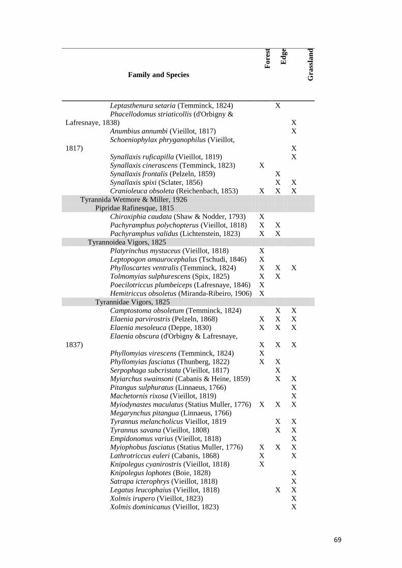
69

Family and Species

Fo

rest

Ed

ge

Gra

ssla

nd

Leptasthenura setaria (Temminck, 1824)

X

Phacellodomus striaticollis (d'Orbigny &

Lafresnaye, 1838)

X

Anumbius annumbi (Vieillot, 1817)

X

Schoeniophylax phryganophilus (Vieillot,

1817)

X

Synallaxis ruficapilla (Vieillot, 1819)

X

Synallaxis cinerascens (Temminck, 1823) X

Synallaxis frontalis (Pelzeln, 1859)

X

Synallaxis spixi (Sclater, 1856)

X X

Cranioleuca obsoleta (Reichenbach, 1853) X X X

Tyrannida Wetmore & Miller, 1926

Pipridae Rafinesque, 1815

Chiroxiphia caudata (Shaw & Nodder, 1793) X

Pachyramphus polychopterus (Vieillot, 1818) X X

Pachyramphus validus (Lichtenstein, 1823) X X

Tyrannoidea Vigors, 1825

Platyrinchus mystaceus (Vieillot, 1818) X

Leptopogon amaurocephalus (Tschudi, 1846) X

Phylloscartes ventralis (Temminck, 1824) X X X

Tolmomyias sulphurescens (Spix, 1825) X X

Poecilotriccus plumbeiceps (Lafresnaye, 1846) X

Hemitriccus obsoletus (Miranda-Ribeiro, 1906) X

Tyrannidae Vigors, 1825

Camptostoma obsoletum (Temminck, 1824)

X X

Elaenia parvirostris (Pelzeln, 1868) X X X

Elaenia mesoleuca (Deppe, 1830) X X X

Elaenia obscura (d'Orbigny & Lafresnaye,

1837) X X X

Phyllomyias virescens (Temminck, 1824) X

Phyllomyias fasciatus (Thunberg, 1822) X X

Serpophaga subcristata (Vieillot, 1817)

X

Myiarchus swainsoni (Cabanis & Heine, 1859)

X X

Pitangus sulphuratus (Linnaeus, 1766)

X

Machetornis rixosa (Vieillot, 1819)

X

Myiodynastes maculatus (Statius Muller, 1776) X X X

Megarynchus pitangua (Linnaeus, 1766)

Tyrannus melancholicus Vieillot, 1819

X X

Tyrannus savana (Vieillot, 1808)

X X

Empidonomus varius (Vieillot, 1818)

X

Myiophobus fasciatus (Statius Muller, 1776) X X X

Lathrotriccus euleri (Cabanis, 1868) X

X

Knipolegus cyanirostris (Vieillot, 1818) X

Knipolegus lophotes (Boie, 1828)

X

Satrapa icterophrys (Vieillot, 1818)

X

Legatus leucophaius (Vieillot, 1818)

X X

Xolmis irupero (Vieillot, 1823)

X

Xolmis dominicanus (Vieillot, 1823)

X

70

Family and Species

Fo

rest

Ed

ge

Gra

ssla

nd

Passeri Linnaeus, 1758

Corvida Wagler 1830

Vireonidae Swainson, 1837

Cyclarhis gujanensis (Gmelin, 1789) X X X

Vireo chivi (Linnaeus, 1766) X X X

Corvidae Leach, 1820

Cyanocorax caeruleus (Vieillot, 1818)

X X

Cyanocorax chrysops (Vieillot, 1818) X

Passerida Linnaeus, 1758

Hirundinidae Rafinesque, 1815

Pygochelidon cyanoleuca (Vieillot, 1817)

X

Progne tapera (Vieillot, 1817)

X X

Tachycineta leucorrhoa (Vieillot, 1817)

X

Troglodytidae Swainson, 1831

Troglodytes musculus (Naumann, 1823)

X X

Polioptilidae Baird, 1858

Polioptila dumicola (Vieillot, 1817)

X

Turdidae Rafinesque, 1815

Turdus flavipes (Vieillot, 1818) X X X

Turdus rufiventris (Vieillot, 1818) X X X

Turdus amaurochalinus (Cabanis, 1850) X X X

Turdus subalaris (Seebohm, 1887) X X

Turdus albicollis (Vieillot, 1818) X X

Mimidae Bonaparte, 1853

Mimus saturninus (Lichtenstein, 1823)

X

Motacillidae Horsfield, 1821

Anthus hellmayri (Hartert, 1909)

X

Thraupidae Cabanis, 1847

Saltator similis (d'Orbigny & Lafresnaye,

1837) X

X

Saltator aurantiirostris (Vieillot, 1817)

X X

Nemosia pileata (Boddaert, 1783)

X

Pyrrhocoma ruficeps (Strickland, 1844) X

Lanio cucullatus (Statius Muller, 1776)

X

Lanio melanops (Vieillot, 1818) X

Tangara sayaca (Linnaeus, 1766) X X X

Tangara preciosa (Cabanis, 1850) X X

Stephanophorus diadematus (Temminck,

1823) X X X

Paroaria coronata (Miller, 1776)

X

Pipraeidea melanonota (Vieillot, 1819) X X

Pipraeidea bonariensis (Gmelin, 1789)

X

Emberizidae Vigors, 1825

Zonotrichia capensis (Statius Muller, 1776)

X X

Ammodramus humeralis (Bosc, 1792)

X

Haplospiza unicolor (Cabanis, 1851)

X

Donacospiza albifrons (Vieillot, 1817)

X

Poospiza nigrorufa (d'Orbigny & Lafresnaye,

X

71

Family and Species

Fo

rest

Ed

ge

Gra

ssla

nd

1837)

Poospiza cabanisi (Bonaparte, 1850) X X

Sicalis flaveola (Linnaeus, 1766)

X

Sicalis luteola (Sparrman, 1789)

X X

Emberizoides herbicola (Vieillot, 1817)

X

Emberizoides ypiranganus (Ihering & Ihering,

1907)

X

Embernagra platensis (Gmelin, 1789)

X

Sporophila caerulescens (Vieillot, 1823)

X

Cardinalidae Ridgway, 1901

Cyanoloxia brissonii (Lichtenstein, 1823)

X

Parulidae Wetmore, Friedmann, Lincoln, Miller,

Peters, van Rossem, Van Tyne & Zimmer 1947

Setophaga pitiayumi (Vieillot, 1817) X X X

Geothlypis aequinoctialis (Gmelin, 1789)

X

Basileuterus culicivorus (Deppe, 1830) X X

Myiothlypis leucoblephara (Vieillot, 1817) X X

Icteridae Vigors, 1825

Cacicus chrysopterus (Vigors, 1825) X X

Pseudoleistes guirahuro (Vieillot, 1819)

X

Agelaioides badius (Vieillot, 1819)

X

Molothrus bonariensis (Gmelin, 1789)

X

Fringillidae Leach, 1820

Sporagra magellanica (Vieillot, 1805) X X X

Euphonia chlorotica (Linnaeus, 1766) X X

1

2

3

4

5

6

72

1

Appendix Figure 2: Traits that maximized the correlation between functional 2

community patterns and the habitat types, in forest (FO), forest edges (ED), and 3

grassland (GR) habitats. Different letters indicate significant differences between 4

forest, edges and grassland. 5

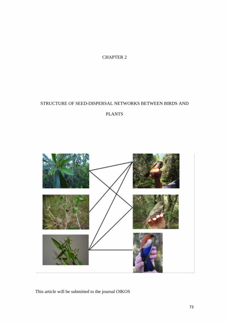
73

CHAPTER 2

STRUCTURE OF SEED-DISPERSAL NETWORKS BETWEEN BIRDS AND

PLANTS

This article will be submitted to the journal OIKOS

74

Structure of seed-dispersal networks between birds and plants

Grasiela Casas1,*, Pâmela V. Friedemann1 and Valério D. Pillar1




Abstract:

Mutualistic plant–animal interactions are vital for ecosystem functioning as they play

a central role in plant reproduction (i.e. dispersal and pollination). Understanding the

structure and dynamics of mutualistic interactions is essential for biodiversity studies

and allows the investigation of ecological and evolutionary mechanisms. Our goal

was to investigate the structure of seed-dispersal networks between plants and birds.

For this purpose, we analysed 19 seed dispersal networks between plants and birds, of

which two were described in the current study and 17 obtained from literature. We

described the generalized mutualistic network patterns such as nestedness,

connectance, modularity and degree distribution. We sampled two of these networks

in areas of forest-grassland mosaic in Southern Brazil. The most important birds as

disperser that we found in the two collected networks were generalists. Those birds

were found in every environment type of our study areas (forest, forest edge and

grassland) and they probably play an important role in the process of forest expansion

into grasslands. Additionally, we found a nested structure in almost every network

studied, suggesting that interactions among plants and birds show some robustness to

random species extinctions. Most of our datasets were not modular, which might

indicate that seed dispersal has low interaction specificity, but our result is not

consistent enough to assume a pattern (only 10 from 19 seed dispersal networks were

not modular). The lack of modularity could also be an effect of network size, since

most of the datasets used were small networks (less than 100 species). The truncated

power law fit was prevalent in most networks, suggesting the role of constraints

(forbidden links) in potential interactions shaping seed dispersal mutualistic

networks. Our findings suggest the existence of an apparent common assembly

process occurring in seed dispersal mutualistic networks, regardless the differences in

sampling methodology or continents where the networks were sampled.

Keywords: frugivory, interactions, mutualistic networks, Southern Brazil.

75

Introduction 1

2

Mutualistic interactions between plants and animals are vital for ecosystem 3

functioning as they play a central role in plant reproduction through seed dispersal 4

and pollination mechanisms (Wright 2002), and the life histories of animals by 5

influencing community dynamics and diversity (Jordano et al. 2003). Most tropical 6

plant species depend on animals to disperse their seeds (Howe and Smallwood 1982), 7

and seed dispersal by vertebrates is crucial. In areas with forest-grassland mosaics, 8

bird-dispersers are especially important for the process of forest expansion as they 9

contribute to the initial phase of nucleation of trees as diaspore carriers from forest to 10

grassland (Duarte et al. 2006). 11

Network theory facilitates the understanding of the structure and dynamics of 12

mutualistic interactions, as well as the ecosystem impact of the loss of interactions 13

and species extinctions (Bascompte and Jordano 2007). Understanding network 14

structure is essential for studying biodiversity and allows the investigation of 15

ecological and evolutionary mechanisms. However, coevolutionary processes can be 16

expected to diverge between mutualistic and antagonistic networks, and 17

consequently, their structural patterns are expected to be different as well (Lewinsohn 18

et al. 2006). Thus, the dynamic and stability of networks constrain the existing 19

structure of mutualistic and trophic networks toward opposite patterns (Thébault and 20

Fontaine 2010). In the past, more studies have dealt with comparison of mutualistic 21

networks than with antagonistic networks (Miranda et al. 2013) with pollination 22

being the most investigated network type so far. 23

The most basic structure described in ecological networks is connectance 24

(Dunne et al. 2002), which is the proportion of links observed relative to the possible 25

76

amount of links that could exist in a network. Mutualistic networks are often nested 1

(Bascompte et al. 2003), creating a pattern where specialist species (species with few 2

interactions) interact with other species that interact with both specialists and 3

generalists (species with many interactions). Nested and connected networks may be 4

more resistant to species loss because species with few interactions are probably 5

connected to generalist species which tend to be more tolerant to environmental stress 6

(Bastolla et al. 2009). 7

Connectivity can also be characterized by the distribution that describes the 8

probability of finding a species within a certain number of interactions which is 9

called “degree distributions” (Jordano et al. 2003). The statistical properties of degree 10

distributions have important consequences for the interpretation of the processes 11

underlying ecological networks (Otto et al. 2007). Complex networks often vary in 12

their structure, having a frequency distribution of vertex connectivity (i.e., number of 13

links per species) that decays as a scale-free (power-law), broad-scale (i.e., truncated 14

power-law distributions) or faster-decaying functions (i.e., exponential) (Amaral et al. 15

2000). Networks that fit the power law distribution are described as heterogeneous, in 16

which the bulk of the nodes have a few links, but a few nodes are more connected 17

than randomly expected. Truncated power law means that as the number of 18

interactions reaches an average value, the probability of finding more connected 19

species drops faster than expected in a power-law. In contrast, in exponential fits, the 20

probability of a node having a number of links larger than the average drops very fast 21

(Bascompte and Jordano 2007). Jordano et al. (2003) explored the organization of 22

mutualistic networks and found that are often characterized by a few super-23

generalists species, while the majority of species establish just a few interactions. 24

Some mutualistic networks are also modular, i.e., subsets of species interact 25

77

more frequently among themselves than with other species in the community. 1

Modularity is assumed to increase stability in pollination networks, because 2

cascading disturbances are expected to spread more slowly through a modular than a 3

non-modular structure (Olesen et al. 2007). For seed dispersal networks, the 4

coexistence of modular networks has been also reported (Mello et al. 2011, Vidal et 5

al. 2014), nevertheless modularity has been little investigated in seed dispersal 6

networks. On the other hand, mutualistic networks have been shown to be less 7

modular than antagonistic networks, while modularity seems to decrease their 8

persistence when compared to trophic networks (Thébault and Fontaine 2010). 9

Our goal is to investigate the structure of seed-dispersal networks between 10

plants and birds, using the metrics of nestedness, modularity, connectance and degree 11

distribution. We utilized collected data from two seed dispersal networks in Southern 12

Brazil and another 17 seed dispersal networks obtained from the literature (including 13

one network also sampled in Southern Brazil) to describe mutualistic network 14

patterns. 15

16

Methods 17

18

Study area of collected networks 19

Study areas were located in two physiographic regions of the state of Rio Grande 20

do Sul, Southern Brazil, Campos de Cima da Serra (CCS) and Serra do Sudeste (SS) 21

(Figure 1). CCS is located in the Atlantic Forest biome, whereas SS is located in the 22

Pampa biome. Each area is composed of mosaics of vegetation that include grassland, 23

forest and other less representative vegetation types. In the Pampa biome, grasslands 24

cover large continuous areas and forests are mostly restricted to riparian zones, 25

78

whereas in Atlantic Forest grasslands are located in the highlands of the South-1

Brazilian Plateau. The CCS is located between 450 m and 900 m above sea level, and 2

SS is between 100 m and 350 m. We sampled two areas each in the CCS and SS 3

regions. 4

Fire and grazing by domestic animals are considered to be the principal factors 5

impeding expansion of forest over grassland vegetation in the past centuries and 6

under current climatic conditions (Pillar and Quadros 1997). Management of the 7

study areas included cattle ranching occurring in both grasslands and forest patches, 8

with grazing pressure less intense in CCS than SS, since the sampling in CCS 9

occurred inside the two nature reserves: Tainhas State Park and the Aparados da 10

Serra National Park. 11

12

13 Figure 1. Rio Grande do Sul state with South America and Brazil insert; map of the 14

dominant vegetation physiognomies of Southern Brazil (IBGE 2004). Numbers 15

represent the study locations in CCS (1 and 2) and SS (3 and 4) areas. 16

17

18

79

Bird sampling and seed collection 1

We captured birds placing eight mist nets in forest interiors (with ≥ 100 m 2

distance from edges in three areas and ≥ 50 m for one area) and another eight in 3

forest-grassland edges. We captured, identified, banded, and maintained birds in 4

restraining bags for at least 20 minutes to collect faeces during three mornings 5

(weather permitted) in all four seasons between August 2012 and May 2013. In total, 6

we sampled 215 hrs in each environment (forest and forest edge). If we multiply the 7

total hours by eight mist nets, we sampled in each environment 1,720 hrs. 8

Seeds found in fecal samples were identified to species, when possible, to build 9

an interaction matrix between birds and the plant that they consumed, considering the 10

number of interaction events (the number of times that a specific bird species 11

consumed a specific plant species). To facilitate the process of seed identification, 12

fruiting plants were also collected in the study area in the same period of bird 13

sampling. These collected seeds were compared to local herbaria for identification. 14

In the same areas that birds were captured, we also recorded the abundance of 15

bird species through point counts in forest environments and forest edges (three point 16

counts in each environment) (Casas and Pillar, unpub. data, Chapter 1). All 17

individuals seen and/or heard were accounted for, except those that only flew over 18

the area. 19

Plant species composition data were obtained by another study carried out at 20

the same areas (Gliesch-Silva 2015). Each local unit (two per area) consisted in 140 x 21

70 m, divided into two plots of 70 x 70 m located in the forest and grassland areas 22

right at the forest edge with evidence of forest expansion, i.e., with the presence of 23

woody individuals over grassland. Fifteen circular sub-plots of 100 m2 were randomly 24

distributed and sampled, where all woody plant individuals with DBH≥5 cm (DBH - 25

80

diameter at breast height) were measured. At the forest edge the woody individuals 1

measured were with DGH≥5 cm (DGH - diameter at ground height). In our study, 2

plant and bird abundance was used to construct the graph 3D where nodes were 3

proportional to abundance of species. 4

5

Datasets 6

To compare the structure between our collected networks with other seed-7

dispersal networks, we analysed 14 published and three unpublished datasets 8

(quantitative and qualitative, i.e., only representing the presence or absence of a given 9

interaction), including one other seed dispersal networks collected in Southern Brazil 10

(Table 1). Two of those datasets were obtained from the Interaction Web Database 11

(http://www.nceas.ucsb.edu/interactionweb/), and 14 from the web of life 12

(http://www.web-of-life.es/). 13

14

Table 1: Description of the 19 plant-frugivore networks. Information about dataset 15

source, habitat type, location, data type, methodology approach and the number of 16

species of birds and plants are given. 17

Code Dataset Habitat type Location Data type Methodology Bird Plant

BA Baird

(1980)

Oak-hickory, red

maple and

floodplain forest

Princeton,

Mercer,

New Jersey,

USA

Number of

times a

specific bird

species was

observed

eating a

specific plant

fruit

Transects 21 7

CA

Carlo et al.

(2003)

Subtropical

secondary forests

Frontón,

Puerto Rico

Number of

interactions

observed on a

plant

Focal bird

species

15 21

CO Cordillera,

Puerto Rico 13 25

CG Caguana,

Puerto Rico 16 25

CI Cialitos,

Puerto Rico 20 34

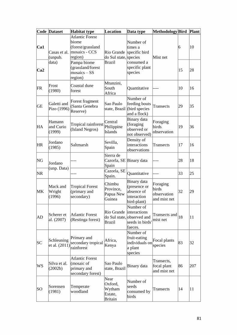
http://www.nceas.ucsb.edu/interactionweb/

http://www.web-of-life.es/

81


Ca1

Casas et al.

(unpub.

data)

Atlantic Forest

biome

(forest/grassland

mosaics - CCS

region) Rio Grande

do Sul state,

Brazil

Number of

times a

specific bird

species

consumed a

specific plant

species

Mist net

6 10

Ca2

Pampa biome

(grassland/forest

mosaics – SS

region)

15 28

FR Frost

(1980)

Coastal dune

forest

Mtunzini,

South

Africa

Quantitative ---- 10 16

GE Galetti and

Pizo (1996)

Forest fragment

(Santa Genebra

Reserve)

Sao Paulo

state, Brazil

Number of

feeding bouts

(bird species

and a flock)

Transects 29 35

HA

Hamann

and Curio

(1999)

Tropical rainforest

(Island Negros)

Central

Philippine

Islands

Binary data

(foraging

observed or

not observed)

Foraging

birds

observation

19 36

HR Jordano

(1985) Saltmarsh

Sevilla,

Spain

Density of

interactions

observations

Transects 17 16

NG Jordano

(unp. Data)

----

Sierra de

Cazorla, SE

Spain

Binary data ---- 28 18

NR ---- Cazorla, SE

Spain. Quantitative ---- 33 25

MK

Mack and

Wright

(1996)

Tropical Forest

(primary and

secondary)

Chimbu

Province,

Papua New

Guinea

Binary data

(presence or

absence of

interaction

bird-plant)

Foraging

birds

observation

and mist net

32 29

AD Scherer et

al. (2007)

Atlantic Forest

(Restinga forest)

Rio Grande

do Sul state,

Brazil

Number of

interactions

observed and

seeds in birds'

faeces.

Transects and

mist net 18 11

SC Schleuning

et al. (2011)

Primary and

secondary tropical

rainforest

Africa,

Kenya

Number of

fruit-eating

individuals on

a plant

species

Focal plants

species 83 32

WS Silva et al.

(2002b)

Atlantic Forest

(mosaic of

primary and

secondary forest)

Sao Paulo

state, Brazil Binary data

Transects,

focal plant

and mist net

86 207

SO Sorensen

(1981)

Temperate

woodland

Near

Oxford,

Wytham

Estate,

Britain

Number of

seeds

consumed by

birds

Transects 14 11

82


MT

Wheelwrig

ht et al.

(1984)

Montane Forest

(area surrounding

by forest,

woodlots and

pastures)

Monteverde

, Costa Rica Binary data

Transects,

mist net, and

focal plant

and bird

species

40 169

1

2

Data analysis 3

For the 19 seed dispersal networks, we explored nestedness, connectance, 4

modularity, degree of distributions and the medium degree for plants and animal (see 5

below). All analyses of network metrics (except for modularity) were performed with 6

bipartite package (Dormann et al. 2008) using the R platform (R Core Team 2013). 7

Nested networks are characterized by a core of highly connected species 8

(generalists) that interact mainly with each other, and a group of specialist species 9

that interact mainly with the generalist species (Bascompte et al. 2003). We assessed 10

nestedness by computing the metric NODF (Almeida-Neto et al. 2008), which 11

corrects biases resulting from matrix fill and matrix dimensions. NODF values of 0 12

indicate non-nestedness and 100 perfect nesting. We used nested function in bipartite 13

package. 14

Connectance (C) is the proportion of links observed in a network relative to the 15

possible amount of links (Dunne et al. 2002), with values from 0 to 1. For bipartite 16

networks it is calculated as C=L/ (I x J), were L is the number of realized links; I and 17

J are the number of species of each party in bipartite networks, e.g., plants and 18

animals. The species degree is the number of different species that a certain species 19

interacts with. We also calculated the medium degree for plants and birds for each 20

network. 21

Modularity is characterized by the existence of groups of nodes (species), that 22

interact more among each other than with other groups (modules) in a network 23

83

(Guimera and Amaral 2005). It ranges between 0 (random network with no 1

modules) to 1 (maximum modularity). We calculated modularity with the 2

MODULAR program (Marquitti et al. 2014). To calculate nestedness and modularity 3

significance we used the model 2 (Bascompte et al. 2003) as null model, which 4

generates networks in which the probability of two species to interact depends on the 5

number of interactions of both species in the real network. 6

Degree distribution can be described as the probability of finding a species 7

with a certain number of interactions (Jordano et al. 2003). We examine the 8

cumulative distributions P(k) of the number of interactions per species, k, fitting three 9

different models: exponential, P(k) ~ exp (– k); power-law, P(k) ~ k–; and truncated 10

power-law, P(k) ~ k– exp (– k ⁄ kx), where is the fitted constant (degree exponent) 11

and kx is the truncation value. The crucial step for this analysis is how often an 12

exponential, power-law or truncated power-law provides the best fit to the data. We 13

calculated the degree distributions with the degreedist function in bipartite package 14

and for the species of each trophic level separately. The Akaike Information Criterion 15

(AIC) was used to evaluate which model provided the best fit. 16

For the networks that we sampled the contribution of each bird species in 17

relation to each plant species from which it consumed resources was assessed, using 18

the importance index (I). The importance index was calculated as in the equation 19

below: 20

Ij = Σ[(Cij/Ti)/S], 21

where i is the plant species, j is the bird species, Ti is the total number of birds 22

species feeding on the plant species i, S is the total number of plants species included 23

in the sample, Cij corresponded to the binary data, with 1 if bird species j consumes 24

the fruits of plant species i, and 0 if it does not. The same importance index was used 25

84

to evaluate the importance of each plant species on the diet of bird dispersers, where i 1

is the bird species and j the plant species. This index varies from 0 to 1, and tends to 2

1 when a bird disperser (or plant species) has many interactions in the community or 3

has a large number of exclusive interactions (Murray et al. 2000, Silva et al. 2002). 4

5

Results 6

7

Datasets 8

The 19 seed dispersal networks we analysed (including the two sampled for this 9

study) ranged in size from 16 to 293 species and had different sampling 10

methodologies (transects, focal plants and/or mist net) and sampling intensities. 11

Connectance ranged from 0.05 to 0.69 and the medium degree of both birds and 12

plants ranged from 1.40 to 16.65. Almost all networks exhibited a significantly nested 13

structure (Table 2). Also, ours results pointed towards a relationship between 14

connectance and network size. We tested, through Spearman rank correlation 15

analysis, the relationship between connectance and network size and found a 16

significant inverse relationship (rS=-0.75, P<0.005, n=19). Nine networks were 17

significantly modular, and we found a prevalence of truncated power-law model 18

(Table 2, Figure 2). 19

20

21

Table 2: Descriptors of the 19 plant-frugivore networks: NODF- nested overlap and 22

decreasing fill; CON- connectance; MOD- modularity; Pl D. and An D.- plant and 23

bird degree distributions respectively; K.M Pl and K.M An– Medium Degree of both, 24

plants and birds. 25

Code Size NODF CON MOD Pl D. An D.

K.M

Pl

K.M

An

Ca1 16 14.39NS 0.23 0.55 NS NF NF 2.33 1.40

SO 25 45.92*** 0.3 0.32 NS TR NF 4.18 3.29

85

FR 26 74.57*** 0.69 0.12** TR PL/TR 6.88 11.00

BA 28 50.98* 0.34 0.31 NS TR EX/TR 7.14 2.38

AD 29 49.82* 0.25 0.34 NS PL-TR EX/TR 2.83 4.63

HR 33 78.76* 0.44 0.22* EX-TR EX/TR 7.56 7.12

CA 36 34.17* 0.16 0.47* PL-TR EX 2.43 3.40

C0 38 29.69* 0.34 0.50* TR TR 1.96 3.77

Ca2 43 27.31* 0.12 0.53 NS PL-TR NF 2.04 3.50

CG 41 44.7* 0.17 0.39 NS EX-TR EX/TR 2.72 4.25

NG 46 61.52* 0.26 0.27 NS EX-TR EX/TR 7.17 4.61

CI 54 43.38* 0.14 0.38 NS NF EX/TR 2.79 4.75

HA 55 37.37NS 0.29 0.37* TR TR 5.47 10.37

NR 58 58.98* 0.18 0.31** TR TR 6.00 4.55

MK 61 11.21* 0.07 0.65*

PL-TR-

EX PL/TR 2.28 2.06

GE 64 35.49* 0.14 0.37* EX/TR TR 4.17 5.03

SE 121 34.58* 0.14 0.31 NS TR TR 12.70 4.76

MT 209 32.87* 0.1 0.40* TR TR 3.94 16.65

WS 293 17.06* 0.05 0.34 NS TR TR 5.42 10.19

*, P<0.005; **, P<0.05, ***,P=0.05; NS, not significant. Degree of distributions: TR, truncated 1 power-law; EX, exponential; PL, Power-law; NF, No Fit (no model fitted the distributions of links 2 per species well). 3

4

Networks sampled in the current study 5

From 480 bird individuals sampled in our two networks, 112 individuals 6

presented seeds in their faeces, distributed in 21 species of passerine birds and 38 7

bird-dispersed plants of woody and non-woody plants species (16 not identified) 8

(Figure 3). Mainly in Ca2 network, bird and plant species that had more links (i.e., 9

higher “degree”) were also the more abundant species (Figure 3). We analysed this 10

relationship between plant and bird abundance and degree using Spearman’s rank 11

correlation. The abundance and degree of plants and birds were significantly 12

correlated for Ca2 network (birds: rS=0.53, P=0.04, n=15; plants: rS=0.41, P=0.02, 13

n=28), but not for Ca1 network (birds: rS=0.44, P=0.37, n=6; plants: rS=0.04, P=0.90, 14

n=10). 15

86

1

Figure 2: Cumulative distribution of connectivity (number of links per species, k, or 2

degree) for 18 seed dispersal interaction networks. Panels show the cumulative 3

distributions of species with 1, 2, 3, ..., k links (dots), exponential fits (light gray), 4

power-law fits (gray lines) and truncated power-law fits (black lines). See network 5

codes in Table 1. We do not show network Ca1 because no model fitted the 6

distributions of links per species. 7

87

1

2 Figure 3: Seed dispersal networks sampled in Rio Grande do Sul state, Brazil (Ca1 3

and Ca2 respectively). Node size is proportional to abundance of species and link 4

width is proportional to the number of interaction events. Red nodes depict plant 5

species, whereas yellow nodes are bird species. Bird species lables: Bale- Basileuterus 6

leucoblepharus, Chca- Chiroxiphia caudata, Cych- Cyanocorax chrysops, Elpa- Elaenia 7

parvirostris, Elme- Elaenia mesoleuca, Elsp- Elaenia sp., Kncy- Knipolegus cyanirostris, 8

88

Myma- Myiodinastes maculatus, Pavi- Pachyramphus viridis, Syru- Syndactyla 1

rufosuperciliata, Tapr- Tangara preciosa, Tasa- Tangara sayaca, Tual- Turdus albicollis, 2

Tuam- Turdus amaurochalinus, Turu- Turdus rufiventris, Viol- Vireo olivaceus, Zoca- 3

Zonotrichia capensis. Plant species lables: Bato- Banara tomentosa, Cist- Cissus striata, 4

Dara- Daphnopsis racemosa, Dran- Drimys angustifolia, Euun- Eugenia cf. uniflora, Euur- 5

Eugenia uruguaiensis, Ilsp- Ilex sp., Libr- Lithraea brasiliensis, Masp- Maytenus sp., Misp- 6

Miconia sp., Mypa- Myrcia palustris, Myat- Myrrhinium atropurpureum, Mysp- Myrsine sp., 7

Myrt- Myrtaceae, Posa- Pouteria salicifolia, Scle- Schinus lentiscifolius, Scbu- Scutia 8

buxifolia, Stle- Stirax leprosus, Trac- Tripodanthus acutifolius, Mo- morph, plant species 9

where the seeds could not be identified. Image produced with FoodWeb3D, written by 10

R.J. Williams and provided by the Pacific Ecoinformatics and Computational 11

Ecology Lab (http://www.foodwebs.org). 12

13 14

The two bird species with higher importance index were the same for Ca1 and 15

Ca2 network: Turdus albicollis and T. rufiventris (Figure 4 and Figure 5), that 16

together represented 50% of total from importance index. Elaenia flycatchers were 17

placed in the third position in both networks. The most common species of Elaenia 18

changed according to the physiography region, with Elaenia mesoleuca in CCS 19

region and E. parvirostris in SS region, but in both, Elaenia flycatchers were the 20

most abundant. The important index of plant species as suppliers of fruit resources 21

differed between the two networks: in Ca1 the most important species were Scutia 22

buxifolia and Ilex sp., and in Ca2 Myrsine sp. and Scutia buxifolia. In both networks, 23

the two plant species represented 38% of the total importance index. Myrsine sp. 24

appeared in Ca1 in fifth place. These plants species also differed in abundance in the 25

phytosociological sampling between regions. Scutia buxifolia was the third most 26

abundant plant species in SS region (Ca2 network), while in CCS region (Ca1 27

network) only three individuals were recorded in all local units sampled. In CCS 28

Myrsine sp. was the second most abundant plant species and in SS region the sixth. 29

30

31

http://www.foodwebs.org/

89

1

Figure 4: Importance index (I) of the Ca1 network for the bird species as dispersers 2

and for plant species suppliers of fruit resources for birds. Network sampled in Rio 3

Grande do Sul state, Campos de Cima da Serra region, Brazil. 4

5

90

1

Figure 5: Importance index (I) of the Ca2 network for the bird species as dispersers 2

and for plant species suppliers of fruit resources for birds. Network sampled in Rio 3

Grande do Sul state, Serra do Sudeste region, Brazil. Morph = plant species where 4

the seeds could not be identified. 5

6

7

91

The Ca1 network was smaller than Ca2, with size of 16 species. It showed 14 out 1

of the 60 possible interactions and had connectance C=0.23. This smallest network 2

was not significantly nested (Table 2) and we also could only poorly estimate the 3

degree distribution of this network due to the small sample size. The Ca2 network 4

showed 52 out of the 420 possible interactions and had connectance of C =0.12. It 5

exhibited a significantly nested structure fitting a truncated power-law model for 6

plants, although no model fitted the distributions of links per bird species (Figure 2). 7

Neither of the networks were modular (Table 2). 8

9

Discussion 10

11

We analysed the structural properties of two seed dispersal networks we 12

collected in Southern Brazil and another 17 networks obtained from the literature. We 13

reported that seed dispersal mutualistic networks showed a common assembly pattern 14

regarding nestedness, connectance, and degree distributions. 15

There is a debate on the implications of nestedness for the stability and 16

persistence of species within networks, with studies concluding that nestedness 17

promotes stability (Bastolla et al. 2009, Thébault and Fontaine 2010) or imperils 18

species persistence (Allesina and Tang 2011). However, as found in our and previous 19

studies (Bascompte et al. 2003, Thébault and Fontaine 2010), mutualistic networks 20

are highly nested and this cohesive pattern likely provides alternative routes for 21

system responses to perturbations (Bascompte et al. 2003). The asymmetrical pattern 22

in nested networks, with specialist species interacting only with generalists, can 23

provide pathways for rare species to persist (Jordano 1987). The smallest network 24

that we studied (Ca1) was not significantly nested, and both Ca1 and Ca2, were not 25

92

modular. However, a relationship between network size and nestedness and 1

modularity has been reported (Olesen et al. 2007). Bascompte et al. (2003) found, for 2

plant-frugivore and plant-pollinator networks, that with sizes above 28 and 50 species 3

respectively, all networks were significantly nested. In our datasets, only two 4

networks were not significant nested, including one with more than 28 species (HA 5

network with size 55 and Ca1 network with 16 species). Since most of our seed 6

dispersal networks comprise more than 28 species, we cannot suggest an influence of 7

network size on nestedness. 8

We found that connectance and network size were negatively correlated in most 9

of the analysed networks. Our results seem to fit the general pattern reported for seed 10

dispersal networks (Mello et al. 2011). However, the results for connectance, as well 11

as those found for nestedness, have to be interpreted with caution due to the influence 12

of sampling bias in these metrics (Rivera-Hutinel et al. 2012). The small size of the 13

Ca1 network probably was due to the limitation of the method, where the local 14

topographic conditions and taller trees resulted in few interactions registered by the 15

mist nets capture method. However, the mist net interaction has the advantage in 16

relation to the focal plant method because we registered in fact the birds that are 17

dispersing plants species through their faeces. In areas such as where Ca1 network 18

was sampled, maybe a combination of mist net in more than one forest strata could 19

probably find more interactions. 20

The existence of a modular structure has been reported for other seed dispersal 21

networks (Mello et al. 2011, Vidal et al. 2014) and for pollination networks (Olesen 22

et al. 2007). The mutualistic modules hypothesis (Jordano 1987) proposes that 23

phylogenetically related species tend to form subgroups that play similar ecological 24

roles. Conversely, Donatti et al. (2011) showed that modularity can emerge by a 25

93

combination of trait convergence of phylogenetically unrelated species. Therefore, 1

mutualistic networks have been shown to be less modular than antagonistic networks, 2

such as herbivory, because modularity is expected to increase with link specificity 3

(Lewinsohn et al. 2006), and seed-dispersal networks are characterized by low 4

interaction specificity. In addition, modularity seems to decrease the persistence of a 5

mutualistic network, and nestedness increases its resilience (Thébault and Fontaine 6

2010). However, we found that only 10 from 19 seed dispersal networks were not 7

modular (almost half of our dataset), and we assumed that this result is not consistent 8

enough to assume it is a pattern. Another possible explanation is the influence of 9

network size on modularity. For pollination networks, Olesen et al. (2007) found that 10

all networks larger than 150 species were modular, whereas networks with less than 11

50 species were never modular. In our datasets, only two networks were larger than 12

150 (only one presented a significant modularity). However, we do not know if for 13

seed dispersal networks this minimal network size to infer a pattern would hold true. 14

Connectance can also influence modularity, because if it increases with small 15

network size, the size of the core of links between generalized species also increases, 16

which may reduce the level of modularity (Olesen et al. 2007). 17

We found a prevalence of truncated power law fits in our datasets, similar to 18

the Jordano et al. (2003), which verified the degree distributions to explore the 19

organization of pollination and seed dispersal mutualistic networks. The power law 20

fit is described by a large number of species with few interactions that coexist with a 21

relatively small number of super-generalists. The degree of nodes (species) is 22

important, because each time a new node is introduced, it tends to interact with the 23

most-connected nodes, leading to a kind of “rich-gets-richer process” (Bascompte 24

and Jordano 2007). If this is the only process of link addition building the network, 25

94

generalized power-law distributions of interaction frequencies would be expected 1

(Jordano et al. 2003). Filtering imposed by the biological properties of plant–animal 2

mutualisms (constraints) limits the growth of these interaction networks due to the 3

existence of forbidden links, and confers them a truncated power law fit (broad-scale 4

behavior) (Jordano et al. 2003). A pairwise interaction that is impossible to occur, for 5

example, owing to phenological or size mismatch, is an example of forbidden link in 6

seed dispersal network. However, it has been proposed that the degree distribution 7

can be generated by a random interaction model (Vázquez 2005). 8

Bird species with higher importance index in the sampled networks (Ca1 and 9

Ca2) were Turdus albicollis, T. rufiventris, Elaenia mesoleuca and E. parvirostris. 10

This result was similar to those showed by Scherer et al. (2007), a seed dispersal 11

network also collected in Southern Brazil. These bird species occurred in all 12

environmental types in our study areas (forest, forest edge and grassland) (Casas and 13

Pillar, unpub. data, Chapter 1), and are probably important in the expansion process 14

of forest over grasslands in these mosaic areas. These species probably contribute for 15

the resilience to species loss of the network, since species with few interactions and 16

generally more sensitive, are usually connected to generalist species, providing 17

robustness to the network (Bascompte and Jordano 2007, Thébault and Fontaine 18

2010). The most important plant species considering fruit resources were Myrsine sp., 19

Scutia buxifolia and Ilex sp. These plants have small seeds, thus birds with wide 20

range of beak size can eat them, which may contribute to the importance of these 21

plants on network organization. The identity of the species in the core of a nested 22

network, with the potential to drive the coevolution of the whole network, can change 23

geographically. However, results in different local assemblages of mutualists and part 24

of network structure could be explained by properties at the landscape level 25

95

(Bascompte and Jordano 2007). 1

In seed dispersal networks the relative abundance of species is correlated with 2

their degree (Jordano 1987), suggesting that abundance affects the occurrence and 3

frequency of interactions, because abundant species may interact more frequently and 4

with more species than rare species (Vázquez et al. 2009). Only in the Ca2 network 5

we found correlation between the abundance of species and the number of links 6

(degree). However, the most important species in our two networks, considering the 7

importance index, were not necessarily the most abundant ones. Previous studies 8

found that other factors are important in determining the organization of interacting 9

assemblages, such as phenological overlapping and morphological matches (Stang et 10

al. 2007, Vizentin-Bugoni et al. 2014). The core of the studies that tested the 11

importance of abundance and forbidden links in mutualistic networks was with 12

pollination networks, and similar studies with seed dispersal networks are currently 13

lacking. 14

15

Conclusions 16

17

In conclusion, our findings point out that seed dispersal mutualistic networks 18

apparently show a common assembly pattern regardless of the differences in 19

sampling methodology or continents that these networks were sampled. The nested 20

pattern found in our dataset can suggest that interactions among plants and birds 21

show some robustness to random species extinctions. Most of datasets were not 22

modular, which suggests that seed dispersal has low interaction specificity, but our 23

result is not consistent enough to assume a pattern. However, most of datasets were 24

small networks (less than 100 species), and the lack of modularity could be an effect 25

96

of network size. The truncated power law fit was prevalent in most networks, 1

possibly due to constraints (forbidden links) in potential interactions in shaping these 2

mutualistic networks. 3

4

Acknowledgements 5

6

We thank the Programa de Pós-Graduação em Ecologia – Universidade Federal 7

do Rio Grande do Sul and the Conselho Nacional de Desenvolvimento Científico e 8

Tecnológico (CNPq) for funding. This work is part of the project Biodiversity of 9

grasslands and grassland-forest ecotones in Southern Brazil: ecological basis for 10

conservation and sustainable use (SISBIOTA- Federal funding: 11

MCT/CNPq/MEC/CAPES/FNDCT). The SISBIOTA project adopted a common 12

sampling design for all taxonomic groups, for which we acknowledge the work of 13

Eduardo Vélez. The first author thanks CAPES for a scholarship and for the 14

sandwich internship (Ministry of Education of Brazil, Brasília – DF 70.40-020, 15

Brazil), conducted at the Pacific Ecoinformatics and Computational Ecology Lab, 16

coordinated by Profesor Neo Martinez and the postdoctoral fellow Fernanda 17

Valdovinos. We thank all farm owners that kindly allowed this work to be carried out 18

in their properties, and all local environmental authorities that allowed research in 19

protected areas (Secretaria Estadual do Meio Ambiente and Instituto Chico Mendes 20

de Conservação da Biodiversidade). We also thank all researchers that kindly 21

provided data, especially Adriano Scherer for network data, and Mariana Gliesch 22

Silva and Rodrigo Bergamin for the phytososiological data. We thank the 23

ornithologist André Mendonça Lima for the help with bird banding, and many 24

botanists that helped with plant identification: Martin Molz, Rodrigo Bergamin, 25



97

Marcos Carlucci, Guilherme Seguer, Fernanda Schimidt, Ari N. Delmo, and the ICN 1

Herbarium (Herbário do Instituto de Biociências, Universidade Federal do Rio 2

Grande do Sul). 3

4

References 5

Allesina, S., and S. Tang. (2011). Stability criteria for complex ecosystems. Nature 6

483:12. 7

Almeida-Neto, M., P. Guimarães, P. R. Guimarães, R. D. Loyola, and W. Ulrich. 8 (2008). A consistent metric for nestedness analysis in ecological systems: 9 reconciling concept and measurement. Oikos 117:1227–1239. 10

Amaral, L. A. N., A. Scala, M. Barthelemy, and H. E. Stanley. (2000). Classes of 11 small-world networks. Proceedings of the National Academy of Sciences of the 12

United States of America 97:11149–11152. 13

Baird, J. W. (1980). The selection and use of fruit by birds in an eastern forest. 14 Wilson Bulletin 92:63–73. 15

Bascompte, J., and P. Jordano. (2007). Plant-animal mutualistic networks: the 16 architecture of biodiversity. Annual Review of Ecology, Evolution, and 17

Systematics 38:567–593. 18

Bascompte, J., P. Jordano, C. J. Melián, and J. M. Olesen. (2003). The nested 19 assembly of plant-animal mutualistic networks. Proceedings of the National 20 Academy of Sciences of the United States of America 100:9383–9387. 21

Bastolla, U., M. A. Fortuna, A. Pascual-García, A. Ferrera, B. Luque, and J. 22

Bascompte. (2009). The architecture of mutualistic networks minimizes 23 competition and increases biodiversity. Nature 458:1018–1020. 24

Carlo, T. A., J. A. Collazo, and M. J. Groom. (2003). Avian fruit preferences across a 25 Puerto Rican forested landscape: pattern consistency and implications for seed 26 removal. Oecologia 134:119–131. 27

Donatti, C. I., P. R. Guimarães, M. Galetti, M. A. Pizo, F. M. D. Marquitti, and R. 28 Dirzo. (2011). Analysis of a hyper-diverse seed dispersal network: modularity 29 and underlying mechanisms. Ecology Letters 14:773–781. 30

Dormann, C. F., B. Gruber, and J. Frund. (2008). The bipartite package version, 0.73. 31

R Project for Statistical Computing, Leipzig. 32

98

Duarte, L. D. S., M. M. G. Dos-Santos, S. M. Hartz, and V. D. P. Pillar. (2006). Role 1 of nurse plants in Araucaria forest expansion over grassland in south Brazil. 2 Austral Ecology 31:520–528. 3

Dunne, J. A., R. J. Williams, and N. D. Martinez. (2002). Food-web structure and 4

network theory: the role of connectance and size. Proceedings of the National 5 Academy of Sciences of the United States of America 99:12917–12922. 6

Frost, P. G. H. (1980). Fruit-frugivore interactions in a South African coastal dune 7

forest. In: Acta XVII Congressus Internationalis Ornithologici, Berlin, pp.1179-1184. 8

Galetti, M., and M. A. Pizo. (1996). Fruit eating by birds in a forest fragment in 9

southeastern Brazil. Ararajuba 4:71–79. 10

Gliesch-Silva, M. (2015). Functional patterns of woody plants in response to soil and 11

climate gradients in forest-grassland transitions. Master theses, Universidade 12 Federal do Rio Grande do Sul, Brazil. 13

Guimera, R., and L. A. N. Amaral. (2005). Functional cartography of complex 14 metabolic networks. Nature 433:895–900. 15

Hamann, A., and E. Curio. (1999). Interactions among frugivores and fleshy fruit 16 trees in a Philippine submontane rainforest. Conservation Biology 13:766–773. 17

Howe, H. F., and J. Smallwood. (1982). Ecology of Seed Dispersal. Annual Review 18 of Ecology and Systematics 13:201–228. 19

IBGE. (2004). Mapas de Biomas e de Vegetação, Ministério do Planejamento, 20

Orçamento e Gestão, Brasília/DF. 21

Jordano, P. (1985). El ciclo anual de los paseriformes frugívoros en el matorral 22 mediterráneo del sur de España: importancia de su invernada y variaciones 23 interanuales. Ardeola 32:69–94. 24

Jordano, P. (1987). Patterns of mutualistic interactions in pollination and seed 25

dispersal: connectance, dependence asymmetries, and coevolution. American 26

Naturalist 129:657–677. 27

Jordano, P., J. Bascompte, and J. M. Olesen. (2003). Invariant properties in 28 coevolutionary networks of plant-animal interactions. Ecology Letters 6:69–81. 29

Lewinsohn, T. M., P. I. Prado, P. Jordano, J. Bascompte, and J. M. Olesen. (2006). 30 Structure in plant -animal interaction assemblages. Oikos 113(1):174–184. 31

Mack, A., and D. Wright. (1996). Notes on occurrence and feeding of birds at Crater 32

Mountain Biological Research Station, Papua New Guinea. Emu 96:89–101. 33

Marquitti, F. M. D., P. R. Guimarães, M. M. Pires, and L. F. Bittencourt. (2014). 34 MODULAR: Software for the autonomous computation of modularity in large 35

network sets. Ecography 37:221–224. 36

99

Mello, M. A. R., F. M. D. Marquitti, P. R. Guimarães, E. K. V. Kalko, P. Jordano, 1 and M. A. M. de Aguiar. (2011). The modularity of seed dispersal: Differences 2 in structure and robustness between bat- and bird-fruit networks. Oecologia 3 167:131–140. 4

Miranda, M., F. Parrini, and F. Dalerum. (2013). A categorization of recent network 5 approaches to analyse trophic interactions. Methods in Ecology and Evolution 6 4:897–905. 7

Murray, K. G., N. M. Nadkarni, and N. T. Wheelwright. (2000). The importance of 8 different bird species as seed dispersers. Pages: 294-295. In Monteverde: 9 ecology and conservation of a tropical cloud forest. Oxford University Press, 10

New York. 11

Olesen, J. M., J. Bascompte, Y. L. Dupont, and P. Jordano. (2007). The modularity of 12 pollination networks. Proceedings of the National Academy of Sciences of the 13

United States of America 104:19891–19896. 14

Otto, S. B., B. C. Rall, and U. Brose. (2007). Allometric degree distributions facilitate 15

food-web stability. Nature 450:1226–1229. 16

Pillar, V., and F. Quadros. (1997). Grassland-forest boundaries in southern Brazil. 17 Coenoses. Retrieved February 2, 2015, from 18

http://link.springer.com/chapter/10.1007/978-3-0348-8722-9_17. 19

R Core Team. (2013). R: A Language and Environment for Statistical Computing. 20 Retrieved from http://www.r-project.org/. 21

Rivera-Hutinel, A., R. O. Bustamante, V. H. Marin, and R. Medel. (2012). Effects of 22

sampling completeness on the structure of plant-pollinator networks. Ecology 23 93:1593–1603. 24

Scherer, A., F. Maraschin-Silva, and L. R. D. M. Baptista. (2007). Padrões de 25 interações mutualísticas entre espécies arbóreas e aves frugívoras em uma 26

comunidade de Restinga no Parque Estadual de Itapuã, RS, Brasil. Acta 27 Botanica Brasilica 21:203–212. 28

Schleuning, M., N. Blüthgen, M. FlöRchinger, J. Braun, H. M. Schaefer, and K. 29 BÖhing-Gaese. (2011). Specialization and interaction strength in a tropical 30 plant-frugivore network differ among forest strata. Ecology 92:26–36. 31

Silva, W. R., P. De Marco Jr, É. Hasui, and V. S. M. Gomes. (2002). Patterns of Fruit 32 – Frugivore Bird Communities of South-eastern Brazil : Implications for 33 Conservation. Pages 423–435. In D. J. Levey, W. R. Silva, and M. Galetti, 34 editors. Seed Dispersal and Frugivory: Ecology, Evolution and Conservation. 35 Third International Symposium-Workshop on Frugivores and Seed Dispersal, 36

São Pedro, Brazil, 6-11 August 2000. CABI Publishing, São Pedro. 37

Sorensen, A. E. (1981). Interactions between birds and fruit in a temperate woodland. 38

Oecologia 50:242–249. 39

100

Stang, M., P. G. L. Klinkhamer, and E. der Meijden. (2007). Asymmetric 1 specialization and extinction risk in plant-flower visitor webs: a matter of 2 morphology or abundance? Oecologia 151:442–453. 3

Thébault, E., and C. Fontaine. (2010). Stability of ecological communities and the 4

architecture of mutualistic and trophic networks. Science 329:853–856. 5

Vázquez, D. P. (2005). Degree distribution in plant-animal mutualistic networks: 6 Forbidden links or random interactions? Oikos 108:421–426. 7

Vázquez, D. P., N. P. Chacoff, and L. Cagnolo. (2009). Evaluating multiple 8 determinants of the structure of plant-animal mutualistic networks. Ecology 9

90:2039–2046. 10

Vidal, M. M., E. Hasui, M. A. Pizo, J. Y. Tamashiro, W. R. Silva, and P. R. 11

Guimarães Jr. (2014). Frugivores at higher risk of extinction are the key 12 elements of a mutualistic network. Ecology 95:3440-3447. 13

Vizentin-Bugoni, J., P. K. Maruyama, and M. Sazima. (2014). Processes entangling 14 interactions in communities: forbidden links are more important than abundance 15 in a hummingbird-plant network. Proceedings of the Royal Society B: 16

Biological Sciences 281:20132397. 17

Wheelwright, N. T., W. A. Harber, K. G. Murray, and C. Guindon. (1984). Tropical 18 fruit-eating birds and their food plants: a survey of a Costa Rican Lower 19

Montane forest. Biotropica 16:173–192. 20

Wright, J. (2002). Plant diversity in tropical forests: a review of mechanisms of 21 species coexistence. Oecologia 130:1–14. 22

23

24

101

CHAPTER 3

ASSESSING SAMPLING SUFFICIENCY OF NETWORK METRICS USING

BOOTSTRAP

This article will be submitted to the journal Methods in Ecology and Evolution

102

Assessing sampling sufficiency of network metrics using bootstrap

Grasiela Casas1,*, Vinicius A.G. Bastazini1, Vanderlei J. Debastiani1 and Valério D.

Pillar1




Abstract:

Sampling the full diversity of interactions in an ecological community is a highly

intensive effort. Recent studies have demonstrated that many network metrics are

sensitive to both sampling effort and network size. Here, we develop a statistical

framework that aims to assess sampling sufficiency for some of the most widely used

metrics in network ecology, namely connectance, nestedness (NODF- nested overlap

and decreasing fill) and modularity (using the QuaBiMo algorithm), based on

bootstrap methods. Our framework is a resampling technique that can generate

confidence intervals for each network metric with increasing sample size (i.e., the

number of sampled interaction events, or number of sampled individuals), which can

be used to evaluate sampling sufficiency. The sample is considered sufficient when

the confidence limits reach stability or lie within an acceptable level of precision for

the aims of the study. We illustrate our framework with data from three quantitative

networks of plant and frugivorous birds, varying in size from 16 to 115 species, and

17 to 2,745 interactions. The results indicate that, for the same dataset, sampling

sufficiency may be reached at different sample sizes depending on the metric of

interest. The bootstrap confidence limits reached stability, thus the samples were

sufficient for two networks analysed for connectance, nestedness, and modularity.

The sample size of the smallest network was not sufficient for any of the metrics, for

its confidence limit values were wide and unstable with increasing sample size. The

bootstrap method is useful to empirical ecologists to indicate the minimum number of

interactions necessary to reach sampling sufficiency for a specific network metric. It

is also useful to compare sampling techniques of networks in their capacity to reach

sampling sufficiency. Our method is general enough to be applied to different types

of metrics and networks.

Keywords: confidence intervals, ecological networks, bootstrap resampling, sample

size.

103

Introduction 1

2

Network studies have grown extraordinarily in the past few decades, and 3

currently they have mainly focused on the analyses of network structure and 4

robustness (Bascompte and Jordano 2007, Miranda et al. 2013). Understanding the 5

patterns of interaction networks may allow researchers to have a better understanding 6

of ecological and evolutionary mechanisms responsible for these patterns. 7

The most commonly used metrics to describe the structure of plant–animal 8

networks are connectance, nestedness, modularity, and robustness (Dormann et al. 9

2009, Miranda et al. 2013). The most basic structure described in ecological networks 10

is connectance (Dunne et al. 2002), which is the proportion of links observed in a 11

network relative to the possible number of links. Most mutualistic networks are 12

nested, where specialist species interact with subsets of the species interacting with 13

generalists (Bascompte et al. 2003). A highly connected and nested architecture 14

promotes community stability in mutualistic networks, but in trophic networks this 15

stability is enhanced with compartmented (modular) and weakly connected 16

architectures (Thébault and Fontaine 2010). A modular pattern, that is, subsets of 17

species interacting more frequently among themselves than with other species in the 18

community, sometimes prevents the spread of perturbations across the network 19

(Stouffer and Bascompte 2011). 20

Nevertheless, most network metrics are sensitive to sampling effort and 21

network size (Dormann et al. 2009). Studying pollination networks, Olesen et al. 22

(2007) found a relationship between the size of the network and nestedness and 23

modularity. In general, if network size in seed dispersal increases, connectance 24

decreases (Mello et al. 2011). Bascompte et al. (2003) also verified, for plant-25

104

frugivore and plant-pollinator networks, that above a size of 50 species, all networks 1

were significantly nested. Consequently, studies having low sampling effort need to 2

be interpreted with caution (Rivera-Hutinel et al. 2012). However, sampling the full 3

diversity of interactions is a highly intensive effort, and ecologists have now come to 4

realize that most networks published to date may be under-sampled. Chacoff et al. 5

(2012) found that, despite a large sampling effort, their pollination network was 6

under-sampled, as they detected less than 60% of the potential interactions. Relating 7

to seed dispersal mutualistic networks, because most of the published data sets 8

consist on small networks, they may also be insufficiently sampled. 9

To evaluate the accuracy of the sampling procedure in networks, the approach 10

used is manipulating data after sampling. In this regard, the common analyses applied 11

in the literature for mutualistic networks are rarefaction and accumulation curve 12

analyses (Nielsen and Bascompte 2007, Chacoff et al. 2012, Rivera-Hutinel et al. 13

2012). For instance, Martinez et al. (1999) evaluated the relationships between food-14

web properties and richness among taxonomic webs and trophic webs using Monte 15

Carlo simulations and confidence intervals. 16

Although a robust and well-designed sampling procedure is essential for the 17

quality of data, the optimality of sample size and/or intensity effort depends on the 18

objectives of the study (Orloci and Pillar 1989). Probably sampling most of species 19

or interactions in a given area is not necessary to detect a specific pattern in a 20

network. Similarly, the number of interactions needed to reach sampling sufficiency 21

will be different according to the network metrics and the different types of 22

taxonomic groups within mutualistic and antagonistic networks. 23

Here, we developed a statistical framework that aims to assess sampling 24

sufficiency for some of the most used metrics in network ecology based on bootstrap 25

105

resampling. The bootstrap method (Efron 1979, Efron and Tibshirani 1993) is based 1

on the idea that the distribution of observed values in a sample is the best indicator of 2

their distribution in the sampling universe from which the sample was taken. Our 3

framework is very similar to that of Martinez et al. (1999), though our resampling is 4

made according to the bootstrap method with replacement, ultimately mimicking the 5

resampling of the sampling universe. 6

In this paper, we applied bootstrap resampling to evaluate sampling sufficiency 7

for nestedness, modularity, and connectance metrics, using as test cases three 8

quantitative mutualistic networks widely ranging in size. Using the bootstrap method 9

to assess sampling sufficiency for network metrics, we attempted to answer the 10

following question: how many interaction events or number of individuals will need 11

to be sampled in order to reach stability for a given network and network metric? 12

13

Methods 14

15

Bootstrap resampling technique 16

We adapted the method of bootstrap resampling from Pillar (1998) to assess 17

sampling sufficiency for network metrics. Our framework is a resampling technique 18

that can generate confidence intervals for each network metric with increasing sample 19

size (i.e., the number of interaction events sampled), which can be used to evaluate 20

sampling sufficiency (Manly 1992, Pillar 1998). The observed values in a sample are 21

taken as “a pseudo sampling universe”, the best available representation of the actual 22

sampling universe from which the sample was taken: each sample obtained by 23

resampling the sample with replacement is a “bootstrap sample”. The algorithm was 24

the following: 25

106

1) Randomly selects a bootstrap sample of nk interaction events with 1

replacement from the observed sample (pseudo sampling universe) with n interaction 2

events; 3

2) Computes the network metric of interest (θk) for the bootstrap sample and 4

stores the resulting value; 5

3) Repeats steps 1 and 2 a large number of times (say 1,000 times); 6

4) Sorts the values of θk from the smallest to the largest value. Based on this 7

ordering, delimits the confidence limits for a given specified probability α. For 8

example, with 1,000 times and a probability α of 0.05, the lower confidence limit at a 9

given sample size will be the value of θk at the 25th position and the upper limit will 10

be the value of θk at the 976th position. 11

5) Repeats steps 1, 2, 3, and 4 for a new bootstrap sample size nk + δ, where δ is 12

an increase in sample size, repeating the process up to sample size of n interaction 13

events. 14

We also applied the same algorithm considering as sampling units, instead of 15

the interaction events, the captured individuals based on which interaction events 16

were observed. 17

Resampling data according to the bootstrap method will create a frequency 18

distribution for the network metric of interest in samples with increasing size, 19

mimicking the resampling of the sampling universe. The sample is considered 20

sufficient within the range of sample sizes evaluated when the confidence limits 21

reach stability or lie within an acceptable level of precision for the objectives of the 22

study (Pillar 1998). 23

The method described here has been implemented in R (R Core Team 2013), 24

using the package Bipartite (Dormann et al. 2008) to calculate the network metrics. 25

107

The bootstrap function and a script with an example are available as supplementary 1

material. 2

3

Network metrics 4

We assessed sampling sufficiency for three of the most used network metrics: 5

1) Connectance (C), which is the proportion of links observed in a network relative to 6

the possible number of links (Dunne et al. 2002), with values from 0 to 1. For 7

bipartite networks it is calculated as C=L/(I x J), were L is the number of realized 8

links; I and J are the number of species of each part, e.g., plants and animals. 9

Connectance only distinguishes whether links are present or absent (unweighted, 10

binary links), and the information about interaction frequencies is lost. 11

2) Nestedness is characterized by a core of highly connected species (generalists) that 12

interact mainly with each other, and a group of specialist species that interact mainly 13

with the generalist species (Bascompte et al. 2003). We used NODF (nested overlap 14

and decreasing fill) algorithm proposed by Almeida-Neto et al. (2008), which 15

corrects biases resulting from matrix fill and matrix dimensions. Similar to 16

connectance, information about interaction frequencies is lost. NODF ranges from 0, 17

(non-nestedness) to 100 (perfect nesting). 18

3) Modularity is characterized by the degree to which there are groups of nodes 19

(species) that interact more among each other than with other groups (modules) in a 20

network (Guimera and Amaral 2005). We assessed modules using the QuaBiMo 21

algorithm that computes modules in quantitative bipartite networks, based on a 22

hierarchical representation of species link weights and optimal allocation to modules 23

(Dormann and Strauss 2013). It ranges between 0 (random network with no modules) 24

to 1 (maximum modularity). 25

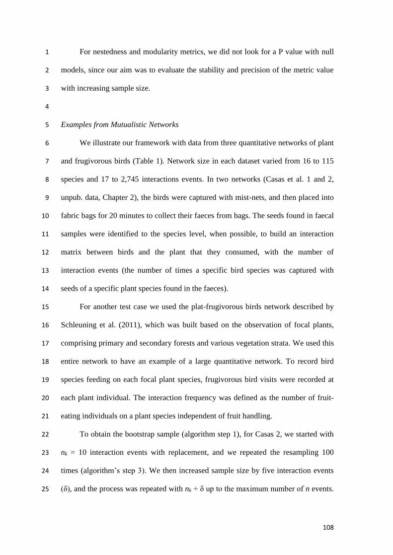
108

For nestedness and modularity metrics, we did not look for a P value with null 1

models, since our aim was to evaluate the stability and precision of the metric value 2

with increasing sample size. 3

4

Examples from Mutualistic Networks 5

We illustrate our framework with data from three quantitative networks of plant 6

and frugivorous birds (Table 1). Network size in each dataset varied from 16 to 115 7

species and 17 to 2,745 interactions events. In two networks (Casas et al. 1 and 2, 8

unpub. data, Chapter 2), the birds were captured with mist-nets, and then placed into 9

fabric bags for 20 minutes to collect their faeces from bags. The seeds found in faecal 10

samples were identified to the species level, when possible, to build an interaction 11

matrix between birds and the plant that they consumed, with the number of 12

interaction events (the number of times a specific bird species was captured with 13

seeds of a specific plant species found in the faeces). 14

For another test case we used the plat-frugivorous birds network described by 15

Schleuning et al. (2011), which was built based on the observation of focal plants, 16

comprising primary and secondary forests and various vegetation strata. We used this 17

entire network to have an example of a large quantitative network. To record bird 18

species feeding on each focal plant species, frugivorous bird visits were recorded at 19

each plant individual. The interaction frequency was defined as the number of fruit-20

eating individuals on a plant species independent of fruit handling. 21

To obtain the bootstrap sample (algorithm step 1), for Casas 2, we started with 22

nk = 10 interaction events with replacement, and we repeated the resampling 100 23

times (algorithm’s step 3). We then increased sample size by five interaction events 24

(δ), and the process was repeated with nk + δ up to the maximum number of n events. 25

109

We started with nk = 7 and used δ = 1 for the smallest network Casas 1 (with only 17 1

interactions events), and nk = 30 and δ = 50 for the largest network Schleuning et al. 2

(2011) (2,745 interactions events). 3

In a second analysis, we used as sample size the actual number of birds 4

captured in our own datasets (Casas 1 and Casas 2). Our aim here was to investigate 5

how many birds are necessary to reach sufficiency for each network metrics. 6

7

Table 1. Description of the three plant-frugivore networks datasets used with the 8

bootstrap resampling technique. 9

Dataset Habitat type Location Data type Methodology Bird Plant

Casas et al.

(unpub.

data)

Atlantic Forest

biome (forest-

grassland mosaics) Rio Grande

do Sul state,

Brazil

Number Ijk of

captures of

bird species j

with seeds of

plant species k

in the faeces

Mist net 6 10

Pampa biome

(grassland-forest

mosaics) 15 28

Schleuning

et al.

(2011)

Primary and

secondary tropical

rainforest Africa, Kenya

Number of

fruit-eating

individuals on

a plant species

Focal plant

species 83 32

10

Results 11

12

The bootstrap confidence limits reached stability for two networks analysed for 13

connectance, nestedness, and for modularity, therefore, samples were considered 14

sufficient for these metrics (Figure 1). The smallest network (Casas 1) did not present 15

sufficiency for any of the analysed metrics, since its confidence limit values were 16

wide and unstable with increasing sample size up to 17 interaction events. For 17

modularity of the Casas 1 network, e.g., the median with the maximum interactions 18

events (17) was expected in 95% of the cases to lie between 0.46 and 0.76, differing 19

by 0.30. This difference is too wide to be indicative of sampling sufficiency 20

110

compared to the other networks (see detailed values of the Figure 1 in Supplementary 1

Material Table 1). 2

The median value of connectance generated by the bootstrap for the second 3

smallest network (Casas 2) reached stability with sample sizes larger than about 90 4

interaction events, but the nested median became stable with sample sizes larger than 5

about 30 events (Figure 1). This means that increasing the sample size beyond 30 6

interaction events did not add new information that could affect the precision of the 7

bootstrap estimation of nestedness. For the largest network (Schleuning et al. 2001), 8

the stability of connectance and nestedness were reached, respectively, with sample 9

sizes larger than about 2,300 and 800 interaction events. When we considered as a 10

separated network only the data collected in secondary forest areas in Schleuning et 11

al. (2011) (with 568 interaction events), we found different results: the stability of the 12

metrics connectance and nestedness were reached with sample sizes larger than 60 13

interaction events (see Supplementary Material Figure 1). For modularity, the results 14

were similar between the two networks from Schleuning et al. (2011). 15

16

Examples with number of bird individuals collected as sample size 17

Using number of individuals as sample size, we found similar results 18

comparing with sample size of number of interactions (Figure 2). Again, the smallest 19

network (Casas 1) did not present sufficiency for any of the metrics analysed, since 20

its confidence limit values were wide and unstable with increasing sample size up to 21

14 captured individuals. The Casas 2 network was considered sufficient for all 22

analysed metrics, as the bootstrap confidence limits reached stability (Figure 2; 23

detailed values of confidence limits, median, and observed metric values of Figure 2 24

is available in Supplementary Material Table 1). 25

111

Results based on number of individual consumers were very similar compared 1

to interaction events because we captured a bird individual, in most cases, with only 2

one plant species in its faeces. Consequently, the matrix using the number of events 3

and the number of individuals captured in our data were very similar (see 4

Supplementary Material Table 2 for Casas 1 matrix with number of events as sample 5

size, and Table 3 for Casas 1 with number of birds captured as sample size). 6

112


Nestedness (NODF) and Modularity metrics obtained by resampling with

replacement method using three quantitative mutualistic networks (plants and

frugivore birds) and number of interaction events as sample size. The 95%

confidence intervals were set based on 100 resampling interactions at each sample

size. See table 1 for detailed information of networks.

113

1

Figure 2. Observed value (star), median and confidence limits of Connectance, 2

Nestedness (NODF) and Modularity metrics obtained by resampling with replacement 3

method using two quantitative mutualistic networks (plants and frugivore birds) and 4

number of bird individuals captured as sample size. The 95% confidence intervals are 5

set based on 100 resampling interactions at each sample size. See table 1 for detailed 6

information of seed-dispersal networks (bird and plant) Casas 1 and Casas 2. 7

8

Casas 1 Casas 2

Number of individuals

Co

nn

ecta

nce

NO

DF

Mo

du

larity

*0.1

0.2

0.3

0.4

0.5

0.6

10 17 24 31 38 45 52 59 66 73 80 87 94

0.2

0.3

0.4

0.5

0.6

0.7

0.8

10 17 24 31 38 45 52 59 66 73 80 87 94

*

*

0.1

0.2

0.3

0.4

0.5

0.6

7 8 9 10 11 12 13 14

*

01

02

03

04

05

06

0

7 8 9 10 11 12 13 14

*

01

02

03

04

05

06

0

10 17 24 31 38 45 52 59 66 73 80 87 94

*

0.2

0.3

0.4

0.5

0.6

0.7

0.8

7 8 9 10 11 12 13 14

114

Discussion 1

2

Our results suggest an important point: sampling sufficiency can be reached at 3

different sample sizes for the same dataset depending on the metric of interest. 4

Nielsen and Bascompte (2007), analysing the sensitivity of connectance and 5

nestedness metrics to variation in sampling effort, also suggested that sampling 6

intensity does not affect all network metrics in the same way, and that nestedness 7

tends to stabilize rapidly with increasing sampling effort. Some median values of 8

metrics generated by the bootstrap reached stability with less than 100 interaction 9

events, meaning that sampling more interaction events probably would have not 10

significantly affected the estimation of this network pattern. 11

However, it has been pointed out that studies of interactions should come from a 12

robust and well-designed sampling procedure, mainly due to the influence of limited 13

sampling effort in network properties (Dormann et al. 2009, Vázquez et al. 2009, 14

Chacoff et al. 2012). In our results, even though the bootstrap confidence limits for 15

some network metrics reached stability in networks with less than 50 species, the 16

range of confidence limits for the largest network (Schleuning et al. 2011), with 115 17

species, was much smaller compared to the other two networks and, consequently, it 18

is considered a more precise sample. Because the study of Schleuning et al. (2011) 19

comprised primary and secondary forests and various vegetation strata, the 20

interactions of this network are heterogeneous (high interaction diversity) and, 21

consequently, the stability for these metrics was reached only with a larger sampling 22

effort compared to the other networks. 23

With the bootstrap method we are looking for the effect of sampling bias on 24

network metrics. In a different way, previous studies used analysis of fieldwork 25

115

sampling techniques to investigate the extent to which conclusions are influenced by 1

the way samples are collected. For example, Gibson et al. (2011) analysed the 2

potential bias in network metrics when using time-based observations or transects in 3

plant-pollinator networks, with rarefaction analysis and null models approach. 4

Analogously, the bootstrap method can be used to compare two methodologies in 5

terms of sampling sufficiency. In seed dispersal networks between plants and birds, 6

e.g., the sampling hours or number of observed plant individuals as sample size 7

(through transect or focal-plant methodologies) can be compared with the number of 8

bird individuals captured (with mist net) that need to be sampled in order to reach 9

stability for each network metric. 10

We assessed sampling sufficiency with the bootstrap method defining sample 11

size as the number of interaction events, and with three mutualistic networks that 12

differed regarding the sampling techniques that were applied to gather the data. Using 13

interaction events, we lose information of the individual interactions, and have only 14

the species interactions, with more dependence between observational units. 15

Independence between sampling units is often an important assumption in data 16

analysis, and the accuracy of the bootstrap method may be affected by lack of 17

independence (Efron and Tibshirani 1993). We used the number of bird individuals 18

captured only with the networks collected by ourselves (Casas et al., unpub. data, 19

Chapter 2). Despite the advantage in using bird or plant individuals observed as 20

sample sizes, the data available for most networks in literature and online databanks 21

unfortunately only allow the extraction of interactions events. 22

Our method to assess the stability and the precision of the estimate of a specific 23

network metric is general enough to be applied to different types of metrics and 24

networks. However, the type of network metric has to provide a single value at the 25

116

end of the analysis. For example, modularity involved an optimization method, but we 1

could use it because it gives a modularity Q value (Dormann and Strauss 2013). 2

Further, since the aim is to evaluate sampling sufficiency of network metrics, the 3

network must be a quantitative one because data with the frequency of interactions are 4

necessary for the resampling of sampling units (interaction events or captured 5

individuals in the test cases). Our method cannot be used for small datasets with less 6

than 10 species considering both trophic levels and less than 7 interaction events. 7

Also, we stress that the bootstrap resampling does not add species and interactions in 8

the network; it only resamples the data with replacement, mimicking the resampling 9

of the presumed sampling universe represented by the observed sample. 10

The bootstrap method can be useful to empirical ecologists, since it shows the 11

minimum number of interaction events (or other defined sampling units) necessary to 12

reach sampling sufficiency for a specific network metric, or allows comparing 13

sampling protocols in terms of effort to reach sampling sufficiency. The concerns on 14

the effect of sampling effort on network metrics in mutualistic (Nielsen and 15

Bascompte 2007, Dorado et al. 2011, Chacoff et al. 2012) and food webs (Goldwasser 16

and Roughgarden 1997, Martinez et al. 1999) have grown in the last few years. We 17

believe that our method is a significant contribution to assess sampling sufficiency in 18

network ecology. 19

20

Acknowledgements 21

22

We thank Programa de Pós-Graduação em Ecologia – Universidade Federal do 23

Rio Grande do Sul and the Conselho Nacional de Desenvolvimento Científico e 24

Tecnológico (CNPq) for funding received. This work is part of the project 25

117

Biodiversity of grasslands and grassland-forest ecotones in Southern Brazil: 1

ecological basis for conservation and sustainable use (SISBIOTA- Federal funding: 2

MCT/CNPq/MEC/CAPES/FNDCT, grant 563271/2010-8). GC thanks CAPES for a 3

scholarship and for the sandwich internship (Ministry of Education of Brazil, Brasília 4

– DF 70.40-020, Brazil), conducted on Pacific Ecoinformatics and Computational 5

Ecology Lab, coordinated by Profesor Neo Martinez, where the first discussion of 6

sampling sufficiency started. VDP has been supported by a productivity fellowship 7

from CNPq (grant 307689/2014-0). 8

9

References 10

11

Almeida-Neto, M., P. Guimarães, P. R. Guimarães, R. D. Loyola, and W. Ulrich. 12 (2008). A consistent metric for nestedness analysis in ecological systems: 13

reconciling concept and measurement. Oikos 117:1227–1239. 14

Bascompte, J., and P. Jordano. (2007). Plant-Animal Mutualistic Networks: The 15 Architecture of Biodiversity. Annual Review of Ecology, Evolution, and 16

Systematics 38:567–593. 17

Bascompte, J., P. Jordano, C. J. Melián, and J. M. Olesen. (2003). The nested 18 assembly of plant-animal mutualistic networks. Proceedings of the National 19 Academy of Sciences 100:9383–9387. 20

Chacoff, N. P., D. P. Vázquez, S. B. Lomáscolo, E. L. Stevani, J. Dorado, and B. 21 Padrón. (2012). Evaluating sampling completeness in a desert plant-pollinator 22

network. Journal of Animal Ecology 81:190–200. 23

Dorado, J., P. Vazquez, Diego, E. L. Stevani, and N. P. Chacoff. (2011). Rareness and 24 specialization in plant-pollinator networks. Ecology 92:19–25. 25

Dormann, C. F., J. Frund, N. Bluthgen, and B. Gruber. (2009). Indices, graphs and 26 null models: analyzing bipartite ecological networks. The Open Ecology Journal 27

2:7–24. 28

Dormann, C. F., B. Gruber, and J. Frund. (2008). The bipartite package version, 0.73. 29 R Project for Statistical Computing, Leipzig. 30

Dormann, C., and R. Strauss. (2013). Detecting modules in quantitative bipartite 31

networks: the QuaBiMo algorithm. arXiv preprint arXiv 1304.3218. 32

118

Dunne, J. A., R. J. Williams, and N. D. Martinez. (2002). Food-web structure and 1 network theory: The role of connectance and size. Proceedings of the National 2 Academy of Sciences of the United States of America 99:12917–12922. 3

Efron, B. (1979). Bootstrap methods: another look at the jackknife. The Annals of 4

Statistics 7:1–26. 5

Efron, B., and R. J. Tibshirani. (1993). An introduction to the bootstrap. Chapman and 6 Hall, London, UK. 7

Gibson, R. H., B. Knott, T. Eberlein, and J. Memmott. (2011). Sampling method 8 influences the structure of plant-pollinator networks. Oikos 120:822–831. 9

Goldwasser, L., and J. Roughgarden. (1997). Sampling effects and the estimation of 10 food-web properties. Ecology 78:41–54. 11

Guimera, R., and L. A. N. Amaral. (2005). Functional cartography of complex 12 metabolic networks. Nature 433:895–900. 13

Manly, B. F. J. (1992). Bootstrapping for determining sample sizes in biological 14

studies. Journal of Experimental Marine Biology and Ecology 158:189–196. 15

Martinez, N. D., B. A. Hawkins, H. A. Dawah, and B. P. Feifarek. (1999). Effects of 16 sampling effort on characterization of food-web structure. Ecology 80:1044–17

1055. 18

Mello, M. A. R., F. M. D. Marquitti, P. R. Guimarães, E. K. V. Kalko, P. Jordano, and 19 M. A. M. de Aguiar. (2011). The modularity of seed dispersal: differences in 20

structure and robustness between bat-and bird-fruit networks. Oecologia 21 167:131–140. 22

Miranda, M., F. Parrini, and F. Dalerum. (2013). A categorization of recent network 23

approaches to analyse trophic interactions. Methods in Ecology and Evolution 24 4:897–905. 25

Nielsen, A., and J. Bascompte. (2007). Ecological networks, nestedness and sampling 26 effort. Journal of Ecology 95:1134–1141. 27

Olesen, J. M., J. Bascompte, Y. L. Dupont, and P. Jordano. (2007). The modularity of 28

pollination networks. Proceedings of the National Academy of Sciences of the 29 United States of America 104:19891–19896. 30

Orloci, L., and V. D. P. Pillar. (1991). On sample size optimality in ecosystem survey. 31 In Computer assisted vegetation analysis. Springer Netherlands. Pages: 41-46. 32

Pillar, V. D. P. (1998). Sampling sufficiency in ecological surveys. Abstracta 33 Botanica 22:37–48. 34

R Core Team. (2013). R: A Language and Environment for Statistical Computing. 35

Retrieved from http://www.r-project.org/. 36

119

Rivera-Hutinel, A., R. O. Bustamante, V. H. Marin, and R. Medel. (2012). Effects of 1 sampling completeness on the structure of plant–pollinator networks. Ecology 2 93:1593–1603. 3

Schleuning, M., N. Blüthgen, M. FlöRchinger, J. Braun, H. M. Schaefer, and K. 4

Böhing-Gaese. (2011). Specialization and interaction strength in a tropical plant-5 frugivore network differ among forest strata. Ecology 92:26–36. 6

Stouffer, D. B., and J. Bascompte. (2011). Compartmentalization increases food-web 7

persistence. Proceedings of the National Academy of Sciences of the United 8 States of America 108:3648–3652. 9

Thébault, E., and C. Fontaine. (2010). Stability of ecological communities and the 10 architecture of mutualistic and trophic networks. Science 329:853–856. 11

Vázquez, D. P., N. Blüthgen, L. Cagnolo, and N. P. Chacoff. (2009). Uniting pattern 12 and process in plant-animal mutualistic networks: a review. Annals of Botany 13 103:1445–1457. 14

15

16

17

18

19

20

21

22

23

24

25

26

27

28

29

30

120

SUPPLEMENTARY MATERIAL 1

2

Supplementary material Table 1: Extension of Figure 1 and 2, in the main text of 3

the paper, and Supplementary Material Figure 1, with details of observed metric 4

values, median and confidence intervals obtained by resampling with replacement 5

method. The values are the 95% confidence intervals (CI) based on 100 resampling 6

interactions only with the maximum number of interaction events for each seed 7

dispersal network. 8

9

10

11

12

Network Metric Observed value Median Upper CI Lower CI Variation of the CI

Casas 2 Connectance 0,12 0,15 0,19 0,12 0,06

NODF 27,32 27,76 37,52 20,91 16,61

Modularity 0,42 0,45 0,53 0,39 0,14


NODF 15,83 11,11 23,91 0,00 23,91

Modularity 0,60 0,64 0,76 0,46 0,30

Schleuning Connectance 0,14 0,13 0,14 0,13 0,02

NODF 33,15 32,04 34,98 30,01 4,97

Modularity 0,23 0,25 0,33 0,15 0,18



NODF 27,32 27,99 39,94 20,14 19,80

Modularity 0,42 0,44 0,50 0,35 0,15


NODF 15,83 11,20 28,43 0,00 28,43

Modularity 0,60 0,60 0,76 0,39 0,37


Schleuning Connectance 0,1857765 0,18143 0,19963 0,16823 0,031405

NODF 33,32811 31,8785 36,445 29,5073 6,93772

Modularity 0,204762 0,259 0,2973 0,18295 0,1143461

FIGURE 1

FIGURE 2

SUPPLEMENTARY MATERIAL FIGURE 1

121

1

Supplementary material Figure 1: Observed value (star), median and confidence 2

limits of Connectance, Nestedness (NODF) and Modularity metrics obtained by 3

resampling with replacement method using Schleuning et al. (2011) mutualistic 4

network with the data collected only in a secondary forest, and number of interaction 5

events as sample size. The 95% confidence intervals are set based on 100 resampling 6

interactions at each sample size. 7

8

9

10

Schleuning

Number of events

Co

nn

ecta

nce

NO

DF

Mo

du

larity

*0

.10

.20

.30

.40

.50

.6

10 60 110 170 230 290 350 410 470 530

*

01

02

03

04

05

06

0

10 60 110 170 230 290 350 410 470 530

*0.2

0.4

0.6

0.8

10 60 110 170 230 290 350 410 470 530

122

Supplementary material Table 2: Example of a matrix (network Casas 1) with 1

interactions events and its dismember matrix used to resampling interactions with 2

replacement according to the bootstrap method. Row represents the code of bird 3

species and columms the plant species. 4

5

6

7

8

9

10

11

Cist Dran Ilsp Libr Masp Misp Myat Mysp Scle Scbu TOTAL

Elme 0 0 0 0 0 1 0 3 0 0 4

Elsp 0 0 1 0 0 0 0 0 0 0 1

Syru 0 0 0 0 0 0 0 0 0 1 1

Tapr 0 0 0 1 0 0 0 0 1 1 3

Tual 1 0 0 2 0 0 1 0 1 0 5

Turu 0 1 0 0 1 0 0 0 1 0 3

1 1 1 3 1 1 1 3 3 2 17

Birds Plants

Elme Misp

Elme MyspElme Mysp

Elme Mysp

Elsp Ilsp

Syru Scbu

Tapr Libr

Tapr Scle

Tapr Scbu

Tual Cist

Tual LibrTual Libr

Tual Myat

Tual Scle

Turu Dran

Turu Masp

Turu Scle

DISMEMBERMATRIX

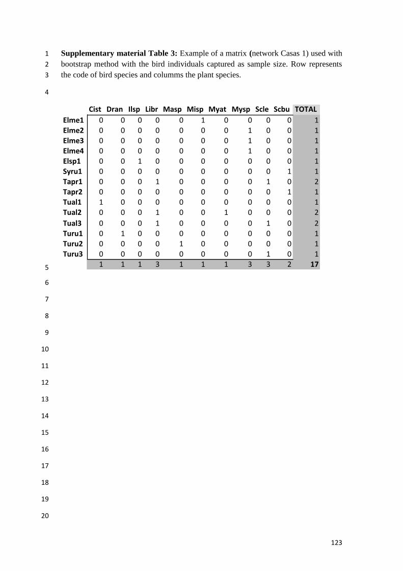
123

Supplementary material Table 3: Example of a matrix (network Casas 1) used with 1

bootstrap method with the bird individuals captured as sample size. Row represents 2

the code of bird species and columms the plant species. 3

4

5

6

7

8

9

10

11

12

13

14

15

16

17

18

19

20

Cist Dran Ilsp Libr Masp Misp Myat Mysp Scle Scbu TOTAL

Elme1 0 0 0 0 0 1 0 0 0 0 1Elme2 0 0 0 0 0 0 0 1 0 0 1

Elme3 0 0 0 0 0 0 0 1 0 0 1Elme4 0 0 0 0 0 0 0 1 0 0 1Elsp1 0 0 1 0 0 0 0 0 0 0 1Syru1 0 0 0 0 0 0 0 0 0 1 1

Tapr1 0 0 0 1 0 0 0 0 1 0 2Tapr2 0 0 0 0 0 0 0 0 0 1 1Tual1 1 0 0 0 0 0 0 0 0 0 1Tual2 0 0 0 1 0 0 1 0 0 0 2

Tual3 0 0 0 1 0 0 0 0 1 0 2Turu1 0 1 0 0 0 0 0 0 0 0 1Turu2 0 0 0 0 1 0 0 0 0 0 1Turu3 0 0 0 0 0 0 0 0 1 0 1

1 1 1 3 1 1 1 3 3 2 17

124

Supplementary material Bootstrap function (boot.net) 1

2 ## Packages 3 4 require(SYNCSA) # for function progressbar 5 require(picante) # for function matrix2sample 6 require(bipartite) 7 8 ## Description 9 10 # The boot.net function assesses sampling sufficiency for network 11 metrics, based on bootstrap methods with replacement. It generates 12 confidence intervals for each network metric with increasing sample 13 size. Here we used as examples connectance, NODF and modularity 14 metrics. 15 16 ## Usage 17 18 # boot.net(web, n.min = 30, by = 10, runs = 1000, method = c("nodf", 19 "connectance", "modularity"), progressbar = TRUE) 20 21 ## Arguments 22 23 # web = interaction matrix 24 # n.min = minimum number of interaction for bootstrap method with 25 replacement 26 # by = number of the sample size that will be increased in each step 27 of the bootstrap method 28 # runs = number of times that the step will be repeated 29 # method = "nodf","connectance" or "modularity" 30 # progressbar = logic argument (TRUE OR FALSE) to show or not the 31 progress bar of the function. Not compatible with RStudio 32 33 ## Value 34 35 # a dataframe with the metrics values, where each column is a sample 36 size (n.min, by, and number maximum of interactions) and row is the 37 result for each bootstrap sample (runs) 38 39 boot.net<-function(web,n.min = 30, by=10, runs = 1000, 40 method=c("nodf","connectance","modularity"),progressbar = TRUE){ 41 if(length(method) > 1){ 42 stop("\n Only one argument is accepted in method \n") 43 } 44 if(!(method=="nodf"|method=="connectance"|method=="modularity")){ 45 stop("\n Invalid method \n") 46 } 47 n.interaction<-sum(web) 48 if(n.min>n.interaction){ 49 stop("n.min greater than number of interactions") 50 } 51 if(!by%%1==0){ 52 stop("by must be an integer") 53 } 54 if(by>n.interaction){ 55 stop("by greater than number of interactions") 56 } 57 n.link<-sum(ifelse(web>0,1,0)) 58 n.row<-dim(web)[1] 59 n.col<-dim(web)[2] 60 web.1<-as.matrix(matrix2sample(web)) 61

125

web.2<-matrix(NA,n.interaction,2) 1 k=0 2 for(i in 1:n.link){ 3 for(j in 1:as.numeric(web.1[i,2])){ 4 k=k+1 5 web.2[k,]<-c(web.1[i,c(1,3)]) 6 } 7 } 8 sample.seq<-seq(n.min,n.interaction,by) 9 if(!length(which(sample.seq==n.interaction))>0){ 10 sample.seq<-c(sample.seq,n.interaction) 11 } 12 RES<-matrix(NA,runs,length(sample.seq)) 13 colnames(RES)<-paste("sample.size.",sample.seq,sep="") 14 k=0 15 l=0 16 nt=length(sample.seq)*runs 17 for(n in sample.seq){ 18 k=k+1 19 i=0 20 while(i<runs){ 21 i=i+1 22 l=l+1 23 web.boot<-matrix(0,n.row,n.col) 24 colnames(web.boot)<-colnames(web) 25 rownames(web.boot)<-rownames(web) 26 sampled<-web.2[sample(1:n.interaction,n,replace=TRUE),] 27 for(j in 1:n){ 28 row.boot<-which(rownames(web.boot)==sampled[j,1]) 29 col.boot<-which(colnames(web.boot)==sampled[j,2]) 30 web.boot[row.boot,col.boot]<-31 web.boot[row.boot,col.boot]+1 32 } 33 web.boot<-34 web.boot[!rowSums(web.boot)==0,!colSums(web.boot)==0, drop=FALSE] 35 if(method=="nodf"){ 36 RES[i,k]<-nestednodf(web.boot, order = TRUE, weighted = 37 FALSE)$statistic[3] 38 } 39 if(method=="connectance"){ 40 RES[i,k]<-networklevel(web.boot,"connectance") 41 } 42 if(method=="modularity"){ 43 log <- capture.output(mod<-computeModules(web.boot, 44 steps=1E6)) 45 if(!is.null(mod)){ 46 RES[i,k]<-mod@likelihood 47 }else{ 48 i=i-1 49 l=l-1 50 } 51 } 52 if(progressbar){ 53 ProgressBAR(l, nt, style = 3) 54 } 55 } 56 } 57 return(RES) 58 } 59 60

126

Supplementary material Table 4: Example of a matrix (network Casas 2) used in the script bellow (object “SS.txt”) of bootstrap method. Row

represents the code of bird species and columms the plant species.

Bato Cist Dara Euun Euur Misp Mypa Mysp Myrt Posa Scbu Stle Trac Mo01 Mo02 Mo03 Mo04 Mo05 Mo06 Mo07 Mo08 Mo09 Mo10 Mo11 Mo12 Mo13 Mo14 Mo15

Bale 1 0 0 0 0 0 0 0 0 0 0 0 0 0 0 0 0 0 0 0 0 0 0 0 0 0 0 0Chca 0 0 0 0 0 0 0 0 0 0 1 0 0 0 0 0 0 0 0 0 0 0 0 0 0 0 0 0

Cyca 0 0 0 0 0 0 0 0 0 1 0 0 0 0 0 0 0 0 0 0 0 0 0 0 0 0 0 0Elpa 1 0 4 0 0 0 0 3 0 0 4 0 0 0 1 0 0 1 0 0 0 0 0 0 1 0 0 0Elsp 0 0 0 0 0 0 0 5 0 0 0 0 0 0 0 0 0 0 0 0 0 0 0 0 0 0 0 0Kncy 0 0 0 0 0 0 0 1 0 0 0 0 0 0 0 0 0 0 0 0 0 0 0 0 0 0 0 0

Myma 0 0 0 0 0 0 0 1 0 0 1 0 0 0 0 0 0 0 0 0 0 0 0 0 0 0 0 0Pavi 0 0 0 0 0 0 0 0 0 0 0 0 0 0 0 1 0 0 0 0 0 0 0 0 0 0 0 0Tapr 1 0 0 0 0 1 0 0 0 0 0 0 1 0 0 0 0 0 0 0 0 0 0 0 0 0 0 0Tasa 0 0 0 0 0 0 0 0 0 0 1 0 0 0 0 0 0 0 0 0 0 0 1 0 0 0 0 0

Tual 11 1 0 0 1 0 2 6 0 0 2 1 0 1 0 0 0 0 1 0 1 1 0 0 0 1 0 0Tuam 0 0 2 0 0 0 4 11 0 0 2 0 0 0 0 0 0 0 0 1 0 2 0 0 0 0 0 0Turu 14 0 0 1 0 0 1 6 1 0 0 0 2 0 0 0 1 0 0 0 3 0 0 1 0 0 1 0Viol 0 0 0 0 0 0 0 1 0 0 0 0 0 0 0 0 0 0 0 0 0 0 0 0 0 0 0 1

Zoca 1 0 0 0 0 2 0 0 0 0 0 0 0 0 0 0 0 0 0 0 0 0 0 0 0 0 0 0

127

Supplementary material Bootstrap script (Example) 1

2 # load packages, sources and files 3 4 require(SYNCSA) 5 require(picante) 6 require(bipartite) 7 8 source("boot_net.r") 9 10 webSS<-read.table("SS.txt",header=T) 11 webSS 12 13 # To calculate the observed metric value (e.g., NODF) 14 15 Obs_nodf<-nestednodf(webSS, order = TRUE, weighted = 16 FALSE)$statistic[3] 17 Obs_nodf 18 19 # To calculate the network metric under assessment for the bootstrap 20 samples with replacement method 21 22 Res_SS_nodf<-boot.net(webSS,n.min=10,by=5,runs=100, 23 method="nodf",progressbar=TRUE) 24 Res_SS_nodf 25 26 # To calculate the median and confidence limits (lower and upper 27 confidence intervals) of the bootstrap samples 28 29 SS_boot_median<-apply(Res_SS_nodf,2,median) 30 SS_boot_median 31 SS_boot_quantile_lower<-apply(Res_SS_nodf,2,quantile,probs=0.025) 32 SS_boot_quantile_lower 33 SS_boot_quantile_upper<-apply(Res_SS_nodf,2,quantile,probs=0.975) 34 SS_boot_quantile_upper 35 36 # To extract the sample size for the plot 37 38 sample.seq<-as.numeric(substr(colnames(Res_SS_nodf),13,100)) 39 sample.seq 40 41 # Plot 42 43 plot(SS_boot_median,type="l",xaxt = 44 "n",ylim=c(0,100),ylab="NODF",xlab="Number of events",las=1) # Draw 45 median 46 points(SS_boot_quantile_lower,type="l") # Draw lower quantile 47 points(SS_boot_quantile_upper,type="l") # Draw lower quantile 48 axis(side = 1, at = 1:length(sample.seq), label = c(sample.seq)) # 49 Add axis values and labels 50 points(length(sample.seq),Obs_nodf,pch="*",cex=3) # Add point for the 51 observed nodf 52 53

128

CONSIDERAÇÕES FINAIS

Esta tese abordou 1) a diversidade taxonômica e funcional de aves, e os padrões

de organização de espécies de aves em comunidades refletindo convergência de

atributos (TCAP: Trait Convergence Assembly Patterns) em transições floresta-

campo, 2) a estrutura de redes de interação ave-planta, e 3) a avaliação de suficiência

amostral de métricas de rede utilizando o método de reamostragem com reposição

bootstrap. As principais conclusões de cada capítulo serão apresentadas a seguir.

A diversidade taxonômica diferiu significativamente somente entre floresta e

borda de floresta, enquanto que floresta e borda diferiram do campo em relação à

diversidade funcional. As áreas de campo apresentaram maior diversidade funcional.

Tais resultados possibilitam inferir que estas duas facetas da diversidade podem

capturar diferentes processos de organização de comunidades ao longo de mosaicos

floresta-campo. No presente estudo, as unidades amostrais em campo variaram de

áreas quase que completamente dominadas por uma paisagem campestre a campos

com árvores esparsas e grandes espécies arbustivas. Essa heterogeneidade de

ambientes provavelmente contribuiu para uma maior diversidade funcional de aves no

campo, considerando os atributos selecionados.

Apesar da importância dos regimes de manejo (pastejo e fogo) para a

conservação dos campos no Sul do Brasil, estes fatores podem ter um efeito de

simplificação na estrutura da vegetação em sub-bosques florestais. A floresta e a

borda não diferiram quanto à diversidade funcional, provavelmente devido à

semelhança na estrutura da vegetação entre estes dois ambientes quando comparados

com o campo. Apesar disto, a composição de espécies de aves diferiu entre todos os

ambientes, o que pode evidenciar uma substituição de espécies ao longo da floresta-

129

borda-campo. O padrão de organização a partir da convergência de atributos (TCAP)

indicou que mecanismos de nicho atuam na organização da comunidade de aves, e

que variáveis ambientais indicadas pelas mudanças na estrutura do habitat ao longo da

transição floresta-campo estão agindo como filtros ecológicos.

Duas redes de interação ave-planta foram coletadas no Rio Grande do Sul na

presente tese. Outras 14 redes de interação ave-planta foram pesquisadas na literatura

(uma também coletada no Rio Grande do Sul) e três redes não são publicadas. Em

relação aos padrões de redes de interação, o presente estudo concluiu que redes de

dispersão de sementes entre ave-planta aparentemente apresentam um processo

comum de organização, mesmo havendo diferenças na metodologia, intensidade de

amostragem e continentes onde as redes foram coletadas. O padrão de aninhamento

encontrado na maioria das 19 redes de interação pode sugerir que interações entre

aves e plantas são robustas à extinção aleatória de espécies. A ausência de

modularidade na maioria das redes pode indicar que redes de dispersão de sementes

entre ave-planta possuem pouca interação específica. No entanto, 10 das 19 redes

analisadas não foram modulares, e esta pequena diferença não é consistente o

suficiente para assumir um padrão. Por outro lado, o tamanho pequeno da maioria das

redes (menos de 100 espécies) pode ter influenciado no resultado obtido para a

modularidade, devido à sensibilidade desta métrica ao tamanho da rede de interação.

Propriedades biológicas em mutualismo entre animal e planta (restrições)

podem agir como filtros e limitar o crescimento da rede de interação devido à

existência de ligações proibidas. Um par de interação que se torna impossível de

ocorrer devido à incompatibilidade fenológica ou em relação ao tamanho do bico e do

fruto, são exemplos de links proibidos em redes de dispersão de sementes. A

predominância da lei de potência truncada (truncated power law) em relação à

130

distribuição do grau provavelmente ocorreu devido a ligações proibidas em interações

potenciais, estruturando estas redes mutualísticas entre ave-planta.

As espécies de aves com maior índice de importância nas duas redes descritas

nesta tese foram Turdus albicollis, T. rufiventris, Elaenia parvirostris e E. mesoleuca.

Como são consideradas generalistas, que ocorrem tanto na floresta, quanto na borda e

nos campos (dados dos pontos de escuta do primeiro capítulo), estas espécies

provavelmente têm maior importância no processo de expansão natural da floresta

sobre o campo. Além disto, tais espécies possivelmente contribuem para a resistência

da rede à perda de espécies, pois as espécies de plantas com poucas interações,

geralmente mais sensíveis, estariam conectadas às aves generalistas, propiciando

assim robustez à rede de interações. As espécies de plantas mais importantes como

fonte de frutos foram Myrsine sp., Scutia buxifolia e Ilex sp.. Estas plantas possuem

sementes pequenas, permitindo que aves com uma ampla gama de tamanho de bico

possam consumi-los, o que provavelmente contribuiu para a importância destas

plantas na organização das redes.

O método proposto para avaliar suficiência amostral em métricas de rede,

utilizando o método de reamostragem com reposição boostrap, pode ser usado com

diferentes tipos de métricas de rede, e a rede de interação a ser usada precisa ser

quantitativa. Tal método foi testado com as métricas aninhamento, conectância e

modularidade. Suficiência amostral pode ser alcançada com diferentes tamanhos

amostrais para o mesmo conjunto de dados, dependendo da métrica de rede de

interesse. Como tamanho amostral foi utilizado o número de eventos de interação. Em

alguns casos, a mediana da métrica gerada pelo bootstrap atingiu estabilidade com um

número amostral menor que 100 eventos. Isto significa que amostrando mais eventos

131

provavelmente não alteraria a precisão da estimativa deste padrão da rede de

interação.

O método também pode ser utilizado para comparar duas metodologias,

utilizando como tamanho amostral o número de aves capturadas (por exemplo, através

de redes de neblina) ou horas de esforço amostral (transecções ou planta focal)

necessários a serem amostrados para atingir suficiência amostral para cada métrica de

rede. O método de reamostragem com reposição bootstrap pode ser útil para ecólogos

empíricos, pois mostra o número mínimo de eventos de interação (ou outra definição

utilizada para unidade amostral) necessário para atingir suficiência amostral para uma

métrica de rede específica. O método entretanto não pode ser utilizado para redes

muito pequenas (com menos de 10 espécies considerando ambos níveis tróficos, e

com menos de sete eventos de interação). Tendo em vista que a maioria das métricas

de redes são sensíveis ao tamanho amostral, a preocupação com este efeito tanto em

redes mutualísticas quanto tróficas, vem crescendo nos últimos anos nos estudos de

rede. O método proposto nesta tese é uma importante contribuição neste tópico.

Retomando a pergunta feita na introdução geral para a rede pequena coletada

(com 16 espécies): “será que esta rede não é aninhada ou o não aninhamento foi

devido ao reduzido tamanho amostral?”. Através do método proposto, foi possível

responder que esta rede não foi suficientemente amostrada para nenhuma das métricas

investigadas, ao contrário da segunda rede, com 43 espécies, que apresentou

suficiência amostral para todas as métricas, pois os limites de confiança gerados pelo

bootstrap alcançaram estabilidade.

O presente estudo inseriu-se no projeto SISBIOTA (“Biodiversidade dos

campos e dos ecótonos campo-floresta no Sul do Brasil: bases ecológicas para sua

conservação e uso sustentável”), abrangendo nove municípios no Rio Grande do Sul.

132

Além de contribuir para o levantamento da biodiversidade de aves nessa região, este

estudo também contribuiu para um banco de dados de atributos funcionais de aves.

Como o projeto SISBIOTA abrangeu diferentes grupos biológicos de fauna e flora

amostrados nas mesmas unidades amostrais, este banco de dados permitirá que novas

abordagens e hipóteses sejam testadas, aprimorando a identificação de padrões

taxonômicos, funcionais e filogenéticos de organização de espécies em comunidades

biológicas características dos campos sulinos e ecossistemas florestais associados.

Documents

PADRÕES DE DIVERSIDADE DE AVES E REDE DE INTERAÇÃO