PAD-80-1 An Actuarial and Economic Analysis of State and ... · PDF fileOf State And Local Government ... _----- DIGEST State and local government pension plans exert ... For the base

BY THE COMFTROLLEi GENERAL /2434 Report To The Chairman, Joint Economic Committee Congress Of The United States

An Actuarial And Economic Analysis Of State And Local Government Pension Plans

At the request of the Joint Economic Com- mittee, GAO estimated the annual cost of future benefit payout to State and local government pension plans. Our analysis of several measures of financial soundness demonstrated an increasing financial burden on these pension plans in the aggregate. An increasing proportion of retirees in population of State and local employees is a basic cause of the problem. Varying the economic parameters does not change this fact, but merely changes the year in which the problem is first evident.

Our analysis is not intended to substitute for a detailed actuarial analysis of the more than 6,600 State and local pension plans, but concentrates on identifying emerging trends that should be brought to the attention of policymakers.

oog7-qi7 PAD-80-1

FEBRUARY 26,1980.

. .

COMPTROLLER GENERAL OF THE UNITED STATES

WASHINGTON. D.C. 20548

B-164292

The Honorable Lloyd M. Bentsen, Jr. Chairman, Joint Economic Committee Congress of the United States

Dear Mr. Chairman:

As p-art of the Special Study on Economic Change, ;he Joint Economic Committee has asked the GAO to estimate the annual cost of future benefit payout to State and local government pension plans. This report presents those estimates. Forecasts of other relevant economic and demographic factors are also presented and compared to benefit payout projections to provide perspective. The effect of these factors on the financial viability of State and local government pension plans in the aggregate is discussed. No recom- mendations are made for action by the Congress.

Copies are also beiny sent to the Pension Task Force, the President's Commission on Pension Policy, the Social- Security Administration, the Department or tabor, and others who participated in our review process.

Comptroller General of the United States

COMPTROLLER GENERAL'S REPORT TO THE CONGRESS

AN ACTUARIAL AND ECONOMIC ANALYSIS OF STATE AND LOCAL GOVERNMENT PENSION FUNDS

DIGEST _-----

State and local government pension plans exert an important and yrowing influence on the United States' economic, social, and political fabric. These plans held roughly $108 billion in assets in 1975, and their management will affect the economic security of the 13 million current participants as well as of future participants.

The number of active employees in plans administered by State and local governments grew from 1.6 million in 1940 to 11.2 million in 1975. The assets in State and local plans as a percentage of total assets of all pension plans grew from 13.6 percent in 1950 to 26 percent in 1975 and grew from 20 percent of all government-administered plans in 1950 to 55.5 percent in 1975. Thus, State and local plan enrollment and assets have increased at an even faster rate than that of all pension plans. (See p. 2.)

CONCLUSIONS

At the request of the Joint Economic Corn- mittee, GAO estimated the annual cost of future benefit payout to State and local government pension plans. Our analysis of several measures of financial soundness showed evidence of an increasing financial burden on State and local government pension plans in the aggregate. In our analysis this problem is caused largely by the increasing proportion of retirees in the population of State and local government employees. Varying the economic parameters does not change this fact but merely changes the year in which the problem is first evident. Furthermore, growth in employment above the levels shown does not seem likely, and the characteristics of the plans were purposely unchanged, since a basic tenet of the review was to see what would happen if current benefit and financing provisions were continued.

Tear Sheet. Upon removal, the report cover date should be noted hereon. PAD-80-01

i

Therefore, under the assumptions of this report a worsening financial status for State and local plans in the aggreyate is certain.

Aggregating plans masks the differences among them. Our projections are driven by large plans, which are generally better funded (94 percent of the employees surveyed by the Pen- sion Task Force were in large plans). Smaller plans, which often are not as well funded, are given less weight. The Pension Task Force report estimated that only 20 percent of State and local employees are enrolled in plans that are fully funded by actuarial standards. A/ Furthermore, a recent GAO report 2/ reviewed 72 State and local government pension plans and found that 53 could not meet the funding standards imposed by the Employee Retirement Income Security Act of 1974 on private pension plans. These facts, combined with the inexorable growth in the proportion of retirees, explain why the financial status of the plans in the aggregate begins to deteriorate in the 21st century. Under some conditions, the decline is more rapid but the conclusion is the same: if present funding practices continue, a deterioration in the financial condition of the plans in the aggregate is likely. The few fully funded plans should remain in good shape, but the numerous poorly funded plans can expect financial difficulty in this century.

METHODOLOGY

Our analysis is not intended to be a substitute for a detailed actuarial analysis of the more than 6,600 State and local pension plans, but rather concentrates on

_-- _-_--

&./The Pension Task Force was created by the Employee Retire- ment Income Security Act of 1974 to study public employee retirement systems. on p. 43, app. II.

See discussion of funding techniques

Z/"Funding of State and Local Government Pension Plans: A National Problem," U.S. General Accounting Office, HR&79-66, August 30, 1979.

ii

identifying emerging trends that should be brouyht to the attention of policymakers. The basic approach was to (1) divide the universe of over 6,600 State and local pension plans into homogeneous subdivisions, (2) develop prototypical plans representing the current characteristics of State and local government employees, (3) forecast employment and salary levels for each subdivision usiny reasonable assumptions about future economic and demographic growth, and (4) create an actuarial model to project cost streams and employment levels for the prototypical plans.

Several scenarios were developed showing the effect of varying the actuarial model's economic and demographic parameters, such as employment growth and the inflation rate. Other scenarios could have been presented showing the effect of varying other parameters, but time and resource constraints prevented further analysis. The projections show what would happen in the aggregate if the conditions that prevailed in the mid-1970s were combined with reasonable assumptions concerning future economic and demographic growth.

Benefit Projections

For the base case assumptions, benefit payments grow steadily through the remainder of the 20th century and then begin to grow more rapidly after the end of the century. (See p. 9.) Total payroll increases steadily, being driven upward mainly by inflation. The ratio of benefits to payroll remains roughly constant throughout the remainder of the 20th century. Benefits begin to grow more rapidly after the year 2000, reaching 17 percent of payroll in 2020. The ratio of retired employees to the total of active and retired employees grows at a roughly linear rate (see p. ll), increasing from 15 percent in 1980 to 24 percent in 2020. These figures indicate an increasing financial burden on State and local government retirement systems.

Tear Sheet

iii

Flow of Funds Analysis

The review's main focus was projecting the cost to State and local government pension plans of future benefit payout. To place benefit payout in perspective, benefit projections were compared to contribution and asset growth projections which allowed a simplified flow of funds analysis.

The base case assumptions show that assets grow throughout the 20th century but at a much lower rate after the year 2000. (See p. 11.) Benefits exceed estimated contributions after 2012. In the 21st century, the ratio of assets to benefits declines steadily until benefits exceed the sum of asset growth and contributions in 2049. This indicates that the plans in the aggregate would not be able to meet obligations from current income. (See p. 14.)

iv

Contents __ ___ __ ..~- ---

Page

DIGEST

CHAPTER

1

2

3

APPENDIX

I

II Model to forecast benefit payments

TABLE

1

2

INTRODUCTION Growth of public pension

plans Growing concern over

pension plan performance Scope of this review

METHODOLOGY Characteristics of prototypes Projection of salary and

employment levels Model to project benefit

payout

RESULTS Basic projections

Benefit projections Flow of funds analysis

The effect of varying some key parameters

Lower employment growth Inflation

Summary and conclusions

Projection of salary and employment levels for State and local government employees

i

1

1

2 3

4 4

5

6

9 9

11 11

14 15 2c 22

24

39

Membership, benefits, and salaries for 1975 for the two prototypes 5

Benefit payout projections base case assumptions 10

TABLE

3

4

5

6

7

8

9

10

11

12

13

14

15

16

Paqe

Flow of funds analysis base case assumptions 13

Benefit payout projections lower growth rate scenario 16

Benefit payout projections zero growth rate scenario 17

Flow of funds analysis lower growth rate scenario 18

Flow of funds analysis zero growth rate scenario 19

U.S. employment and State and local government employment 1960-2020 24

State and local government employment by region and for U.S. for the period 1960-2020 at an interval of five years (in millions) 26

Employment per one million population by region in each functional category of local and State government for 1957, 1967, and 1977 34

Constraints on employment per million by functional category 35

2 The regression coefficients, x and rho

values in the functions fitted in all functional categories of employment in all reyions 37

2 The regression coefficient, E and rho

values in the functions fitted in all the functional forms in all regions for real average annual salaries 38

Membership in State and local retirement systems in 1975 39

General financial characteristics (in billions of dollars) 40

Base case projection assumptions 44

Page FIGURE

1

2

3

4

5

6

Retired employees as a percentage of total 12

Benefit and contribution projections 21

State and local total employment by reyion for the period 1960-2020 at an interval of five years 25

Real average salaries of local and State government employees by region for selected years during the period 1960-2020 28

Population by region 1960-2020 30

Direct and indirect linkages of population and real per capita income to local and State government employment

Real per capita income by region 1960-2020

32

33

CHAPTER 1 --

INTRODUCTION

State and local government pension plans exert a substantial and I:-owing influence on the economic, social, and political fabric of the United States. Recent experience shows their LJrowth in size anii scope to be rapid. Rougk. II/' $108 billion in assets were held by these plans in 1375. I'!1 e way these assets are managed will affect the economic security of the 13 million current participants as well as that of future participants.

The Special Studies on Economic Change Subcommittee of the Joint Economic Committee is directing a study of future economic problems. One goal of the study is to obtain more accurate estimates of future outlays from pension plans and the potential effect of these outlays on the Nation's ecol>oi:;it, resources. The Joint Economic Committee asked us to estimate the cost of benefit payouts to State and local pension plans through the year 2020. We have based our estimates on actuarial and economic analyses of data obtained from the Pension Task Force Survey, the Bureau of the Census, and other sources.

The projections presented here do not pretend to pre- dict future events exactly. Their purpose is to provide a better understanding of emerging financial problems, given reasonable assumptions about future economic and demographic changes. The projections are a result of aggregating all State and local government pension plans into two prototypes. Aggreyating masks differences among plans, but allows a clear look at long-term trends so that problems can be addresse,3 before they become worse. Note, however, that to an extent well-funded plans offset poorly funded plans; even when the plans are financially sound in the aggregate, some plans will be in serious financial straits.

GROWTH OF PUBLIC PENSION PLANS __-- --

The development of employee retirement systems began ih the public sector. Before the turn of the century, groups )! policemen, firemen, and teachers were covered under service- related retirement systems in New York, Boston, and other cities. Over 12 percent of the large State and local plans now in operation were established before 1930.

Social Security was instituted in 1935 but was not c:x- tended to State and local government employees. Nearly on:<- half of large State and local plans were established duri;li

1

1931 to 1950 when Social Security coverage for public employees was being debated. Over one-third of the large plans began or underwent a major restructuring after 1950 when State and local employees were given the option to join the Social Security System. In contrast, nearly two-thirds of the small plans were started after 1950 and nearly one- fourth since 1970.

The number of active employees in plans administered by State and local governments grew from 1.6 million in 1940 to 11.2 million in 1975. The assets held by all pension plans in the U.S. (including Social Security) totaled over $400 billion in 1975, up from $38 billion in 1950. The assets in State and local plans as a percentage of total assets of all pension plans grew from 13.6 percent in 1950 to 26 percent in 1975. As a percentage of all government-administered plans, State and local plans grew from 20 percent in 1950 to 55.5 percent in 1975. Thus, while enrollment and assets in all pension plans have grown substantially, State and local plan enrollment and assets have increased at an even faster rate. This increase is largely the result of the substantial overall growth of State and local government in the last 20 years.

GROWING CONCERN OVER PENSION PLAN PERFORMANCE

As the number of people depending on pensions for future financial security grew, concern developed about the integrity of pension plans. In the 196Os, public awareness was height- ened by news articles describing various abuses by the admin- istrators of pension plans. Few plans actually failed. More frequent were complaints about restrictive age and service requirements, mismanagement of funds, and termination of coverage for employees who were close to retirement.

The closing of the Studebaker plant in South Bend, Indiana, in 1964, which inflicted heavy pension losses on workers, led to congressional hearings. Subsequent hearings on related pension concerns preceded the passage of the Em- ployee Retirement Income Security Act (ERISA) on Labor Day, 1974. Although this law does not require that an employer have a pension plan, it does provide partial protection to the participants in plans by setting standards for partici- pation, vesting, funding, and fiduciary responsibility.

The Congress chose not to include public retirement systems in the provisions of ERISA. Two reasons for this deci- sion were the small number of complaints from public bene- ficiaries and the absence of reliable information about public

2

plans. Howevt-r, the Congress did create the Pension Task Force to investigate public pension plans. Data gathered b;: GAO for the Pension Task Force were a basic data source for this report.

A bill was introduced in the 94th Congress that prompted hearings on public pension systems. Because of its similar- ity to ERISA, it was referred to as the Public Employee Re- tirement Income Security Act. PERISA bills have been intro-- duced in subsequent sessions of Congress, and President Carter has appointed a commission to develop a national policy for both public and private pension plans.

SCOPE OF THIS REVIEW

Our primary source of information is data collected by GAO for the Pension Task Force Report issued in March 1978. We also collected data from the Bureau of the Census, the Bureau of Labor Statistics, and other sources. Chapter 2 discusses our methods of estimating future employment and salary levels of State and local government employees, creating prototypical pension plans, and forecasting the future costs of State and local pension plans.

To place the projections of benefit payouts in perspective, we compared them to projections of contribution and asset growth, which allowed us to make a flow of funds analysis. Chapter 3 summarizes the benefit payout projections and the flow of funds analysis. Several scenarios are presented covering a wide range of economic and demographic assumptions. Data limitations prevented a detailed actuarial analysis; our analysis is descriptive of the general financial conditions of the plans in the aggregate as measured by certain rough measures discussed in Chapter 3.

Appendix I contains information on the projections of State and local government employment and salary levels. Appendix II provides technical information on the development of the model to project benefit payout and other actuarial variables.

3

CHAPTER 2

METHODOLOGY -

We developed our estimates of the future cost of State and local government pension plans by

--dividing the universe of 6,630 State and local pension plans into homogeneous subdivisions and determining the characteristics of the two prototypical plans that could be used to estimate the future costs of all plans;

--forecasting employment and salary levels for each subdivision; and

--creating an actuarial model to project benefit streams for these prototypical plans.

To determine the number and characteristics of the prototypical plans, we analyzed the Pension Task Force survey data and other sources. A/ Forecasts of employment and salary levels for State and local government employees were based on an econometric analysis of historical data from the Bureau of the Census and forecasts from a national economic model. 2/

The characteristics of the prototypical plans and the forecasts of employment and salary levels were used as inputs to the actuarial model that projected benefit payout for State and local government pension plans. We developed the actuarial model for age and service retirees for large plans, and extended the results to the universe of all plans. Social Security benefits are not included in our estimates, because the plans were not integrated with Social Security to any appreciable degree.

CHARACTERISTICS OF PROTOTYPES

A review of the Pension Task Force survey and other material led us to conclude that two prototypes would be necessary-- one representing teachers' plans, another representing those of other State and local government employees. We designed the types to conform initially to data collected by the Pension Task Force survey. The prototypes began in the base year 1975 with the characteristics shown in table 1.

l/See appendix II. -

2/See appendix I. - It was our judgment that historical growth levels would not continue unabated.

4

Table 1

Membership, Benefits, and Salaries -- for 1975 for the Two Prototypes ~--

Characteristics

Active membership

Teachers __-.-__

2,480,772

Other State and local employees

5,333,92J

Retired membership a/ 401,841 788,024

Total benefit payments (millions) $2,300 $3,200

Total payroll (millions) $25,500 $45,100

Average annual salary $10,275 $8,451

a/Age and service retirees only.

Other data sources were used for areas that the Task Force survey did not cover. The age and sex distributions of the active populations were based on the Census Bureau's "Current Population Survey" (January 1978). For age and benefit distributions of the 1975 retirees, we aggregated data from actuarial valuations of certain large State, local, and teachers' retirement systems. Based on a review of 23 large plans conducted by the Pension Task Force, we set the post-retirement cost-of-living adjustments at half the future increases in the cost-of-living index. The Unisex Pension 1974 Table (adjusted for varying male-female ratios and future improvements in mortality) was used for mortality rates. Information on ancillary benefits was obtained from the Census Bureau.

PROJECTION OF SALARY AND EMPLOYMENT mvms

To capture the effect of different growth patterns among different regions of the U.S. and among different categories of State and local employees, we projected salary and employment levels for the four U.S. census regions and for six State and local government employment categories. Employment categories were aggregated into two prototypes for the actuarial model discussed in the next section.

Real per capita income correlates with several factors (such as urbanization, education, real per capita Federal Government transfers) that affect State and local government employment, and therefore is used as a proxy for all these factors. Our econometric model forecasts employment per million population as a function of real per capita income. By constraining the amount of employment per million population, an upper limit to the income effect is achieved, thereby constraining the future growth rate to a level lower than that found in the historical data.

The average annual salary in each employment category of State and local government in each of the six reyions is based on fixed salary scales which are periodically increased for cost-of-living adjustments. Increases in the average nominal salary reflect increases in average years of experience, urbanization, cost of living, productivity improvements, and overall labor market conditions. The average nominal salary in each employment category in each region is considered as a function of two broadly classified cateyories--the cost-of- living index and other factors. Factors other than the cost of living adjustment correlated highly with regional real per capita income, and hence, we used the real per capita income in each region as a proxy for all the independent variables that can explain the variation in the real annual average salary.

The projections of State and local employment and salary levels, along with the national cost-of-living index, were the primary economic and demographic inputs for the actuarial model to project future benefit payout.

MODEL TO PROJECT BENEFIT PAYOUT -

The characteristics of the prototypical plans and the projections of employment and salary levels were used as inputs to the actuarial model to estimate future benefit payout. Within each prototype, we projected benefits for three groups-- persons retired in 1975, active employees in 1975, and new entrants after 1975. Projections of the growth in teachers' and in State and local governments' work forces determined the number of new pension plan entrants needed each year in the future.

To the first group, those retired in 1975, we assigned an initial age and benefit distribution, and then "aged" the group using our assumed mortality rates. A projection of inflation through 2020 was used to give the surviving retirees post-retirement cost-of-living adjustments. The total payroll (average salary times number of employees) was distributed initially amony the active employees using a merit scale to

6

reflect a typical worker's career salary progression, neglecting inflation.

The active employees in 1975 and the new entrants who "survived" to retirement were accorded a benefit using the average benefit formulas constructed from the Task Force data. Retirement ages were spread uniformly over a lo-year period, with the median age determined by a review of actuarial valuations and plan provisions. Entry ages were set at 30 and 34 for the teachers' and the State and local prototypes. Note that they represent the average entry age for a typical retiree and not for a typical new entrant. The benefit formulas, entry ages, and retirement ages resulted in an average replacement ratio (that is, percentaye of final compensation) of 52 percent for teachers and 50 percent for State and local retirees. Final compensation in both prototypes was the average of the last 4 years' salary.

The assumed benefit formulas were applied only to those employees retiring on account of age and service. Further- more, the benefits so generated were confined to the modeled population--that is, large, defined benefit l/ teachers' and State and local pension plans. Before a proTection for all 6,630 plans could be obtained, the benefits had to be increased to take into account ancillary benefits 2/ and those plans (and members) outside the modeled population.

From 1970 to 1975 contributions to State and local pension plans increased but at a slower rate than benefits. As a percentage of payroll, however, contributions stayed roughly constant while benefits grew steadily. The Pension Task Force survey showed that contributions were approximately 15 percent of payroll in 1975 for large plans. For the flow of funds analysis, we assumed that this rate would continue through 2020. This assumption shows what the 1975 contribution level might lead to if allowed to continue unchanged.

i/A defined benefit plan is one in which a participant's benefit is computed by a formula relating such factors as pay, age, and years of service. In contrast, a defined contribution plan is one in which the contribution is fixed and a participant's benefit is determined by such factors as the plan's investment earnings and annuity purchase rates at retirement.

2/Ancillary benefits - include disability and survivor benefits and withdrawal payments. Data were obtained from the Bureau of the Census for 1974 through 1977.

The Pension Task Force survey showed that State and local government pension plans held $108.3 billion in assets in 1975. A rate of return on assets of 7.5 percent L/ was assumed for the base case, and assets were projected by adding contributions and interest income and subtracting benefit payments each year.

Several scenarios were developed showing the effect of varying several key parameters of the actuarial model. The effect of varying the growth rate for State and local government employment is discussed in the text. The effect of varying the inflation rate is discussed only in general terms because of the subjective judgments involved in applying different inflation rates to the model. Other scenarios could be presented showing the effect of varying other parameters, but time and resource constraints prevented further analysis.

------- ----

l/Since the assumed average inflation rate is 7.18 percent - per year for the projection period, a small amount of real growth (that is, growth above the level of inflation) is allowed although this level of growth has not always been achieved in the recent past.

8

CHAPTER 3 -

RESULTS

The review was directed primarily toward projecting the future cost of benefit payout for State and local government pension plans. In the course of the review, projections were also made for the total number of active (contributing) employees, total age and service retirees, and total payroll. Finally, contributions and asset levels were projected to allow a flow of funds analysis that provides perspective for the benefit projections.

BASIC PROJECTIONS

The projection of benefit payout was made using the parameters determined by the analysis of salary and employment levels, the long-term trends estimated by the national economic model, and the basic characteristics of the prototypical plans. The assumptions underlying the national economic model affect the projections of State and local government employment and salary levels. The model's basic economic assumption is that the economy will grow steadily at about 2.5 percent (except for a small downturn in 1980), leading to a balanced Federal budget in the mid-1980s. State and local government employment is projected to continue growing through 2020, but the rate of growth declines sharply after 1990. Nonetheless, employment will increase by 62 percent from 1980 to 2020. (The ratio of State and local government employment to total U.S. population will only increase from 5.3 percent in 1980 to 6.6 percent in 2020.) The average salary in 2020 is 20 times greater than the 1980 salary, the result of an average annual inflation rate of approximately seven percent and a real growth rate of about one percent per year. L/

The elements of the prototypical plans are summarized in chapter 2 and detailed in appendix II. This information is used as a starting point for the projection of benefit payout. The projections show what would happen in the aggregate if the conditions that prevailed in the mid-1970s were combined with reasonable assumptions concerning future economic and demographic growth.

L/The inflation rate is 7 percent after 1995 and is higher before that year. The average annual inflation rate is 7.18 percent overall. Real salary growth also fluctuates with an average annual growth rate of 0.90.

9

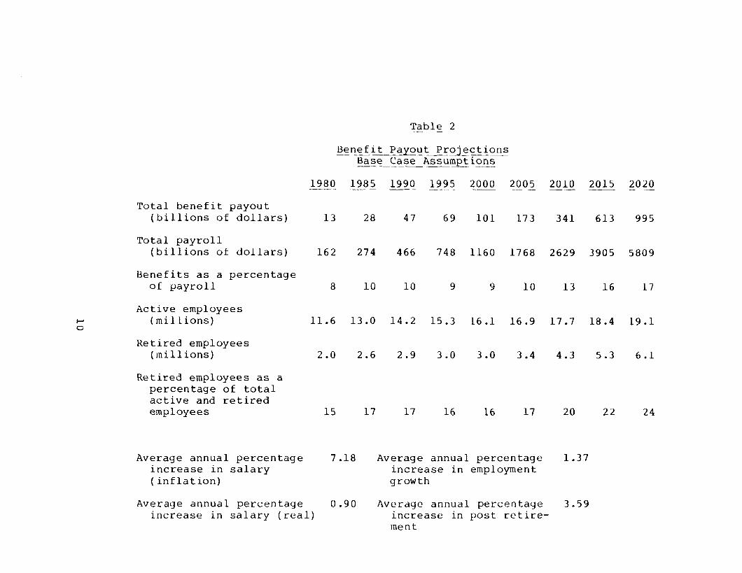
Table 2

Benefit Payout Projections --__ Base Case-Assumotions

---.-L -

P 0

Total benefit payout (billions of dollars)

Total payroll (billions of dollars)

Benefits as a percentage of payroll

Active employees (millions)

Retired employees (millions)

Retired employees as a percentage of total active and retired employees

Average annual percentage increase in salary (inflation)

28 47

274 466

8 10 10

13.0 14.2

2.6 2.9

17 17

7.18 Average annual percentage increase in employment growth

Average annual percentage 0.90 Average annual percentage

1980 -- -

13

162

11.6

2.0

15

1985 1990 1995 --

69

2000 2005

101 173

2010 --

341

2015

613

2020 - --

995

748 1160 1768 2629 3905 5809

9 9 10

15.3 16.1 16.9

3.0 3.0

16 16

3.4

17

13

17.7

4.3

20

16 17

18.4 19.1

5.3

22

6.1

24

1.37

3.59 increase in salary (real) increase in post retire-

ment

Benefit - --- projections .- - ~_~

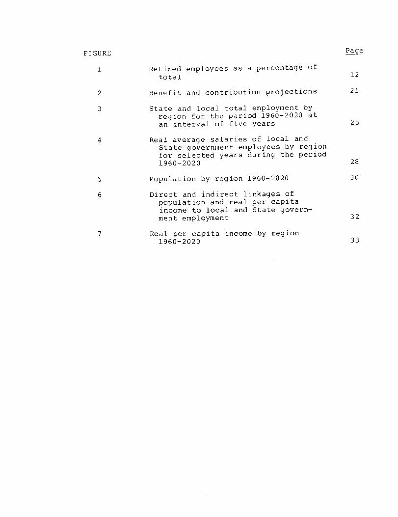
Table 2 shows the basic projections. Benefit payments grow steadily throuyh the remainder of the 20th century and then begin to yrow faster in the 21st century. Total payroll increases steadily, being driven upward primarily by inflation. Benefits as a percentage of payroll remain roughly constant throughout the 20th century and begin increasing after the year 2000, as benefits grow at a more rapid rate. As this ratio increases, the financial burden on State and local government pension systems increases. A steadily increasing ratio of retired employees to the total number of active and retired employees is the basic cause of this phenomenon.

The ratio of retired employees to the total number of active and retired employees yrows at a roughly linear rate except for a period early in the 21st century. L/ As men- tioned in chapter 1, pension plan enrollment grew rapidly beginning in the 1940s until, by 1975, over 90 percent of all government workers were enrolled in public pension plans. During this same period, there was a trend toward early retirement and a yradual increase in the average lifespan in the U.S. These factors helped cause an overall "maturing" of State and local government pension plans as evidenced by the growing proportion of retired members. Figure 1 shows that this trend is forecast to continue through 2020.

Flow of funds analysis __-------.-

To place benefit payout in perspective, we computed a flow of funds analysis. Table 3 shows the results for the base case. Total assets grow throughout, but at a rapidly decreasing rate during the 21st century. Benefit payout exceeds contributions after 2012. The ratio of assets to benefits has been suggested as a rough measure of financial soundness for individual plans, with 15 to 1 or 10 to 1 as a minimal level of funding. 2/ For the base case assumptions,

l-/The downturn around the year 2000 stems from the original distribution of State and local employees. The aye groups 35 through 55 start with roughly the same number of employees. Consequently, fewer of the younger ones actually make it to retirement. Because the possible retirement ages are centered at age 60, there is a significant decline in the number of new retirees in the 199Os, causing a cor- responding decrease in the total number of retirees.

Z/Pension Task Force Report, p. 150.

11

PERCENTAGE 30.0

24.0

18.0

12.0

6.0

0.0

Figure 1

Retired Employees as a Percentage of Total

1970 1980

YEAR

1990 2010 2020-

Assets (billions of dollars)

Percentage growth in assets from previous year

Contributions (billions of dollars)

Benefits (billions of t- W dollars)

Ratio of assets to benefits

Table 3 ~--

Flow of Funds AnalEis __- --- -___- Base Case Assumptions -~-.--~ - ~

1980 1985 -- __-

182 329

14 12

24 40

13 28

14 12

Average annual percentage increase in salary (inflation) a/

Average annual percentage increase in salary (real)

Average annual percentage increase in employment growth

1990 1995 2000 -__ -- --~

562 975 1703

11

68

47

12

12 12 11 9 7

110 170 259 385 572

69 101 173 341 613

14 17 17 14 11

7.18 Average annual percentage increase

in cost of living 3.59

Assumed average annual rate of return on assets 7.50

2005 2010 2015

2913 4648 6757

2020

9231

6

851

995

9

a/1975 is the base year for all forecasts shown in this report.

this ratio begins at 14 to 1 in 1980 and fluctuates throughout the remainder of the 20th century. In the 21st century, it decreases steadily reaching a level of 9 to 1 in 2020. The analysis was continued to 2050 for the base case. After 2020 the ratio of assets to benefits declines steadily until benefits exceed the sum of asset interest and contributions in 2049, showing that the plans in the aggregate would not be able to meet obligations from current income. The projected decline in the ratio of assets to benefits and the fact that benefit payments exceed the sum of asset interest and contributions in 2049 are evidence of a lack of financial soundness in State and local government pension plans in the aggregate. L/

THE EFFECT OF VARYING SOME KEY PARAMETERS

The assumptions used to project the economic and demographic factors are deliberately conservative in the sense that they postpone the financial difficulties caused by the increasing proportion of retirees as discussed previously. The employment growth rate used for our basic analysis allows State and local government employment to continue growing throughout the projection period, though at a much slower rate than recent historical rates of growth. Lowering this growth rate has the effect of making the financial decline occur sooner, in the 20th century.

Further, the inflation rate shown favors the financial soundness of the plans, and the interest rate applied to asset growth is sufficient to allow a small amount of annual real growth. Many State and local government pension funds have not grown more rapidly than the inflation rate in recent years. A lower employment growth rate, inflation rate, or interest rate for asset growth would further exacerbate the financial difficulties.

The characteristics of the prototypical plans used for the benefit projections and the flow of funds analysis are based on our analysis of the Pension Task Force data and other sources and represent typical provisions in the mid-1970s. The effect of lowering the projected growth rate or changing the inflation rate or the manner in which it is applied to the projections is discussed in subsequent sections. Varying

L/This simplified flow of funds analysis cannot be a substitute for a detailed actuarial analysis of the 6,600 individual pension plans. Our analysis concentrates rather on identifying emerging trends that need to be brought to the attention of policymakers.

14

the characteristics of the prototypical plans is not :.lis- cussed: our analysis is designed to show what would happen if the typical characteristics of the pension system in the . 1970s was projected into the future. L/

Lower Employment Growth -- -

For the base case, growth is limited after 1990 by a limit on growth in per capita employment. To test the sensitivity of the projections to a change in the employment level, we developed a second scenario that limits per capita employment in most cases to the averaye level attained by 1980. In this scenario, we curtailed the growth of per capita employment throughout the projection, and employment grew 47 percent from 1980 to 2020. Table 4 shows the estimates. The total number of active employees reaches 16.9 million by 2020 compared to 19.1 million for the base case estimate. Retirees, who are affected less by this change, reach 5.8 million in 2020 instead of 6.1 million.

The number of retirees is affected less than the number of actives because no new entrants are assumed to retire until the 21st century. During the 20th century, the retirees come primarily from the active employees in 1975. The first new employees hired after 1975 take a minimum of 24 years to retire. Growth in the total number of active employees is achieved by adding new entrants. As a result, the forecast number of retired employees remains the same for any scenario until the year 1999, when the effect of new 1975 entrants retiring is first felt.

An extension of the lower growth-rate scenario is a zero growth-rate scenario. Table 5 presents this result, assuminy the 1975 employment level. Retirees as a percentage of the total increase dramatically in this case.

We performed a flow of funds analysis for both the lower- growth and the zero-growth cases. Flow of funds estimates for the lower-growth case (table 6) reveal that benefits exceed contributions after 2010, or 2 years earlier than in the base case, and that the ratio of assets to benefits declines very rapidly in the 21st century, reaching a level of 8 in 2020. -___----

l/The sensitivity to changes in the contribution rate was - tested. If the contribution rate is changed from 14.65 percent of payroll (as shown in the historical data) to 16 percent, the asset to benefit ratio changes from 9 to 1 as shown in Table 3 to 12 to 1 for 2020 and the year in which benefits first exceed contributions changes from 2012 in the base case to 2016.

15

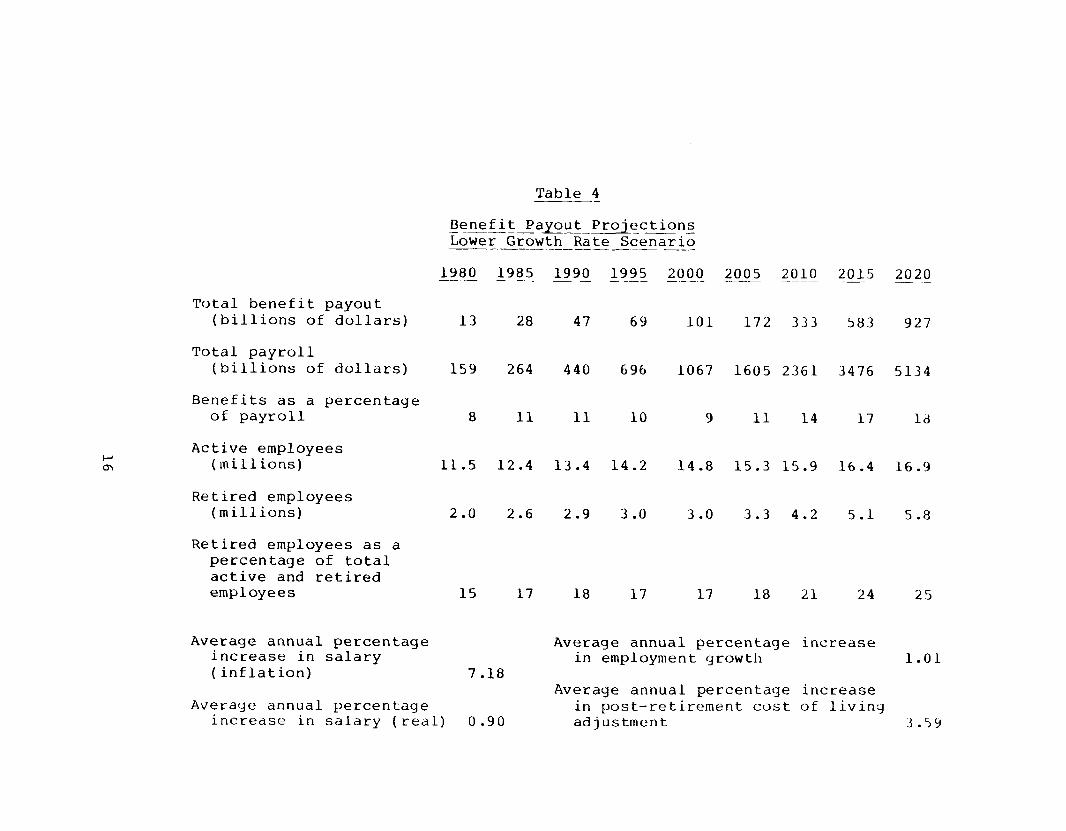
Table 4

Benefit Projections Payout ____ - Lower Growth Rate Scenario --__---- ------I_--.-

Total benefit payout (billions of dollars)

Total payroll (billions of dollars)

Benefits as a percentage of payroll

Active employees (millions)

Retired employees (millions)

Retired employees as a percentage of total active and retired employees


1980 1985 ---.- -__

13 28

159 264

8 11

11.5

2.0

1s

7

12.4

2.6

17

I .18

Average annual percentage increase in salary (real) 0.90

1990 1995 2000 2005 2010 2015 -- --- .-__

47 69 101 172 333 583

440 696 1067 1605 2361 3476

11 10 9 11 14 17

13.4 14.2 14.8 15.3 15.9 16.4

2.9 3.0 3.0 3.3 4.2 5.1

18 17 17 18 21 24


Average annual percentage increase in post-retirement cost of livinrj

2020 _ .~~

927

5134

16.9

5.8

25

1.01

adjustment 3.59

Table 5 ~--

Benefit Payout Pro-Jections -_I- --- Zero Growth Rate Scenario .- ___--

1980

Total benefit payout (billions of dollars) 13

Total payroll (billions of dollars) 148

Benefits as a percentage

P of payroll 9 4

Active employees (millions) 10.4

Retired employees (millions) 2.0

Retired employees as a percentage of total active and retired employees 16



1985 -- -

28

226

12

10.4

2.6

20

7.18

0.90

1990 -__

47

351

13

10.4

2.9

22

1995

69

2000 2005 _-- - __-

10 1 167

2010

299

2015 -- -

478

524 76G 1101 1554 2217

13

10.4

3.0

22

13

10.4

3.0

22

15

10.4

3.3

20

10.4

3.9

24 27

22

10.4

4.3

29


2020

7 !I 1

3191

22

10.4

4.5

30

0 .oo

Average annual percentage increase in ad

post-retirement cost of liviny ustment 3. 59

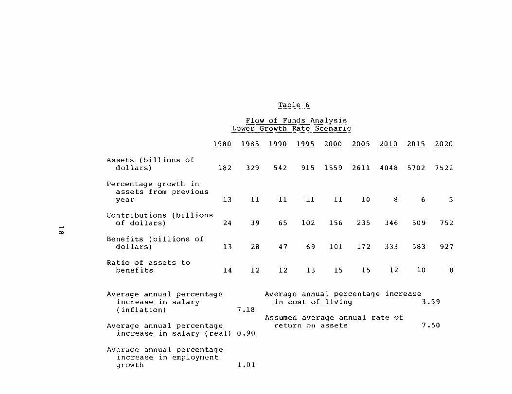
Table 6

Flow of Funds Analysis --. - Lower Growth Rate Scenario __ ---.- --- _ -_~-.__-

Assets (billions of dollars)

Percentage growth in assets from previous year

Contributions (billions of dollars)

Benefits (billions of dollars)

Ratio of assets to benefits

1980 .~

182

13

24

13

14




1985 1990 1995 -- ~-

329 542 915

11

39

28

12

11 11

65 102

47 69

12 13

7.18

Average annual percentage increase in cost of living 3.59

Assumed average annual rate of return on assets 7.50

0.90

1.01

2000 __-

1559

2005

2611

11 10

156 235

101

15

172

15

2010 2015 2020 --- --

4048 5702 7522

8 6 5

346 509 752

333 583 927

12 10 8

Table 7

Flow of Funds Analysis Zero Growth Rate Scenario -__--- _I~ ---

1980 1985 --- -

Assets (billions of dollars) 180 304

Percentage growth in assets from previous year 13 10

Contributions (billions of dollars) 22 33

Benefits (billions of 13 28 I- W dollars)

Ratio of assets to benefits 14 11

Average annual percentage increase in salary (inflation) 7.18

Average annual percentage increase in salary (real) 0.90

Average annual percentage increase in employment growth 0 .oo

1990

465

9

51

47

10

1995 2000 _- --

701 1061

9

77

69

10

9

112

101

11

2005 2010 -- -__

1575 2103

8 5

261 228

167 299

9 7

2015 2020

2404 234')

1

325 467

478 701

5 3

3.59

7.50

Average annual percentage increase in cost of living

Assumed average annual rate of return on assets

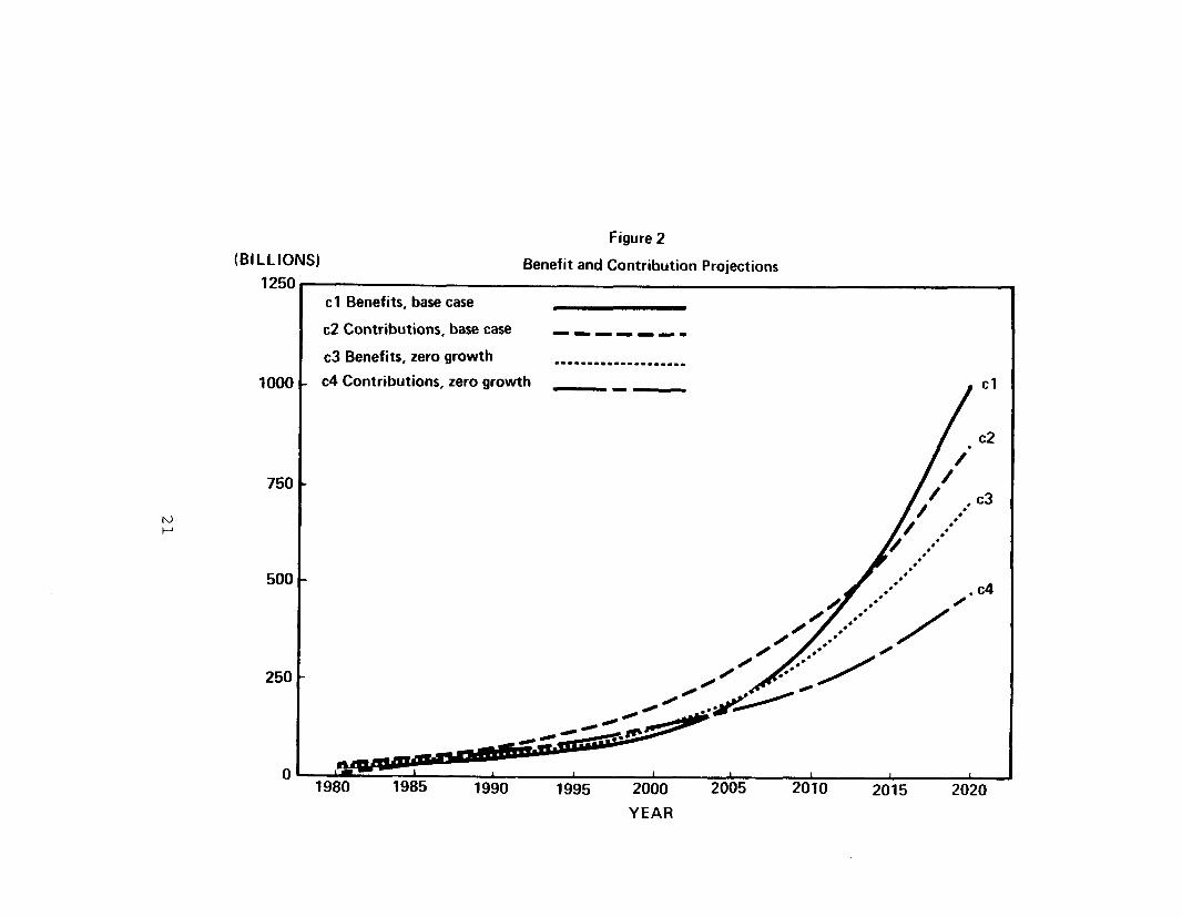
For the zero growth case (table 7), the situation is worse. Lowering the assumed growth rate in State and local government produces a distinct deterioration in the financial condition of the plans in the aggregate. Figure 2 displays this effect.

Inflation

The effect on the forecasts of varying the inflation rate depends on the extent to which the changes in the rate are passed through to the active and retired populations. We based our forecasts of salary increases on historical wage rates adjusted for changes in productivity and the cost of living. A limited survey taken by the Pension Task Force of 23 large retirement systems (with total 1975-76 active membership of 4.5 million) reveals that post-retirement adjustments from 1969 to 1978 averaged about one-half the increase in the Consumer Price Index.

Our analysis of the limited Pension Task Force survey shows that most post-retirement cost-of-living adjustments were either ad hoc or automatic with annual increases. The weighted average of all cost of living adjustments was approximately half the average CPI increase from 1969 to 1978. Accordingly, for the analysis presented in this report, we gave half the annual increase in the cost of living L/ to retirees. Since inflation rates are currently much higher than in the immediate past, it could be argued that employees will demand cost-of-living increases nearer to the inflation rate.

We used a long-term inflation rate of 7 percent. Appro- priate monetary and fiscal policy could lower the rate: however, 7 percent is conservative for our purposes: since only half the cost-of-living increases is passed through the model to retirees, a higher inflation rate increases payroll more than benefits and further delays any difficulties that would be encountered by the plans in the aggregate. Giving retirees a higher percentage of future increases in the cost of living or lowering the projected inflation rate would exacerbate the financial difficulties discussed previously in this chapter. 2/

L/See p. 29 of app. I for a discussion of the cost-of-living index used.

2/Far example, if the inflation rate is changed to an average yearly rate of approximately 4.5 percent and all other paran- eters are unchanged, the ratio of benefits to payroll increases to 22 percent in 2020, up from 19 percent in the b,?se case.

20

(BILLIONS)

1250

Figure 2

Benefit and Contribution Projections

i ooa

750

500

250

a

cl Benefits, base case

c2 Contributions, base case --I---I

c3 Benefits, zero growth . . ..-......-.1......

c4 Contributions, zero growth -- # cl

/

1 -

I -

I -

/

c2

/’

/’

,/ 2. l . c3

/ *.***

1 1

1980 1985 1990 1995

. c4 0

1 i h 1 1

2000 2005 2010 2015 2020

YEAR

SUMMARY AND CONCLUSIONS -.- --- ---

We have concentrated primarily on projecting benefit payout to employees covered by State and local government pension plans through the year 2020. Our base case assumptions estimate that the ratio of benefits to payroll would increase from 8 percent in 1980 to 17 percent in 2020. The ratio of retired employees to the total of retired and active employees increases from 15 percent in 1980 to 24 percent in 2020. These figures indicate an increasing financial burden on State and local government retirement systems.

To place benefit payout in perspective, a simplified flow of funds analysis was also computed. For the base case, the ratio of assets to benefits begins to decline in the 21st century until by 2049 benefits exceed the total of asset growth and contributions, showing that the plans in the aggregate would not be able to meet obligations from current income.

The increasing ratio of benefits to payroll, the decline in the ratio of assets to benefits, and the fact that benefit payout exceeds the sum of asset growth plus contributions in 2049 for the base case are all evidence of an increasing financial burden on State and local government pension plans in the aggregate. In our analysis this problem is caused, to a large extent, by the increasing proportion of retirees in the population of State and local government employees. Varying the economic parameters does not change this fact but merely changes the year in which the problem is first evident. Furthermore, growth in employment above the levels shown does not seem likely and the characteristics of the plans were purposely unchanged. Therefore, under the assumptions of this report a worsening financial status for State and local plans in the aggregate is foreseen.

Aggregating plans masks the differences among them. Our projections are driven by large plans, which are generally better funded (94 percent of the employees surveyed by the Pension Task Force were in large plans). Smaller plans, which often are not as well funded, are given less weight. The Pension Task Force estimated that only 20 percent of State and local employees are enrolled in plans that are fully funded by actuarial standards. L/ Furthermore, a recent GAO

-_-__-.--__

l/See discussion of funding techniques on p. 43 of app. II.

22

report L/ reviewed 72 State and local government pension plans

and found that 53 could not meet the funding standards imposed by ERISA on private pension plans. These facts combined with the inexorable growth in the proportion of retirees explain why key measures of the financial status of the plans in the aggregate begin to deteriorate in the 21st century. Under some conditions, the decline is more rapid but the conclusion is the same: if present funding practices continue, a deterioration in the financial condition of the plans in the aggregate is likely. The few fully funded plans should remain in good shape, but the numerous poorly funded plans can expect financial difficulty in this century.

- --

l/"Funding of State and Local Government Pension Plans: A - National Problem," U.S. General Accounting Office, HRD-79-66, August 30, 1979.

23

APPENDIX I APPENDIX I

PROJECTION OF SALARY AND EMPLOYMENT -- LEVELS FOR STATE AND LOCAL GOVERNMENT EMPLOYEES

State and local government employment and salary levels were estimated based on econometric analysis of long-term economic trends of historical data obtained from the Bureau of the Census. Forecast trends obtained from the Data Re- sources, Inc., national economic model were used as inputs to forecast future employcaent and salary levels. To capture the effect of different growth patterns among different regions of the U.S. and among different categories of the State and local government employees, four regions of the U.S. and six employment categories were considered. Employment categories and regions were aggregated for the actuarial model discussed in appendix II.

Table 8 shows the growth in State and local government employment as forecast by our model. State and local government employment is forecast to increase as a percentage of total U.S. population, but the rate of growth is considerably lower after 1990. The Bureau of Labor Statistics has estimated that total State and local government employment for the U.S. will reach 13.7 million by 1990. The estimate of 14.2 million shown in table 8 compares well with that estimate.

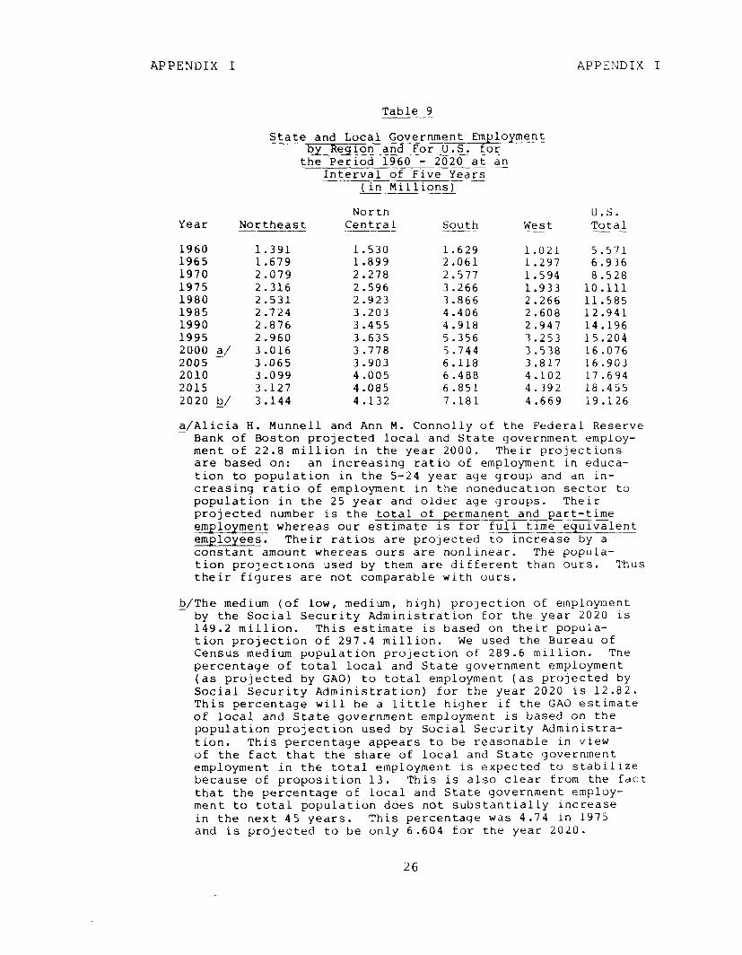
Figure 3 and table 9 show expected total State and local government employment by region for the period 1960 to 2020.

Table 8

Year Population (millions)

Total State and Local Government

Employment (millions)

State and Local Government

Employment as a Percentage of Total

Population

1960 180.4 5.6 3.1 1970 204.1 8.5 4.2 1980 222.0 11.6 5.2 1990 243.3 14.2 5.8 2000 264.1 16 .l 6.1 2010 274.8 17.7 6.4 2020 289.6 19.1 6.6

Source: U.S. population is DRI, State and local employment estimated by GAO.

U.S. Employment and State and Local Government Employment

1960-2020

Total U.S.

24

N ul

TOTAL EMPLOYMENT

(IN MILLIONS)

Figure 3 State and Local Total Employment by Resion . I

for the Period 1960.2020 6.000

7.000

6.000

5.000

4.000

3.000

2.000

1 .ooo

0 1960 1965 1970 1975 1980

LEGEND:

- NORTH EAST

-------a NORTH CENTRAL

- - - SOUTH

-e-*-WEST

0

0 0

0 0

0

0 0

1965 1990

YEARS

1995 2000 2005 2010 2015 2020


Table 9 ---

State and Local Government Employment .- __ by Region and For U.S. for ____--- -

the Period 1960 - 2020 at an --___---- .- Interval of Five Years

(in Millions) __ -__ --

North Year Northeast Central South West - -_-- --~

1960 1.391 1.530 1.629 1.021 1965 1.679 1 .a99 2.061 1.297 1970 2.079 2.278 2.577 1.594 1975 2.316 2.596 3.266 1.933 1980 2.531 2.923 3.866 2.266 1985 2.724 3.203 4.406 2.608 1990 2.876 3.455 4.918 2.947 1995 2.960 3.635 5.356 3.253 2000 $/ 3.016 3.778 5.744 3.538 2005 3.065 3.903 6.118 3.817 2010 '3.099 4.005 6.488 4.102 2015 3.127 4.085 6.851 4.392 2020 y 3.144 4.132 7.181 4.669

U.S. Total __-

5.571 6.936 8.528

10.111 11.585 12.941 14.196 15.204 16.076 16.903 17.694 la.455 19.126

a/Alicia H. Munnell and Ann M. Connolly of the Federal Reserve Bank of Boston projected local and State government employment of 22.8 million in the year 2000. Their projections are based on: an increasing ratio of employment in education to population in the 5-24 year age group and an increasing ratio of employment in the noneducation sector to population in the 25 year and older age groups. Their projected number is the total of permanent and part-time employment whereas our estimate is for full time equivalent employees-. --~-- --

Their ratios are projected to increase by a constant amount whereas ours are nonlinear. The population projections used by them are different than ours. Thus their figures are not comparable with ours.

&/The medium (of low, medium, high) projection of employment by the Social Security Administration for the year 2020 is 149.2 million. This estimate is based on their population projection of 297.4 million. We used the Bureau of Census medium population projection of 289.6 million. The percentage of total local and State government employment (as projected by GAO) to total employment (as projected by Social Security Administration) for the year 2020 is 12.82. This percentage will be a little higher if the GAO estimate of local and State government employment is based on the population projection used by Social Security Administra- tion. This percentage appears to be reasonable in view of the fact that the share of local and State government employment in the total employment is expected to stabilize because of proposition 13. This is also clear from the fact that the percentage of local and State government employment to total population does not substantially increase in the next 45 years. This percentage was 4.74 in 1975 and is projected to be only 6.604 for the year 2020.

26

APPE:JDIX I APPENDIX I

Although total State and local government employment for the U.S. is forecast to almost double between 1375 and 2020, the total employment figure hides significant regional variations. The employment growth rates in the South and West are higher during the period 1960 to 1980 because of the rapid increase in population in these two regions. The growth rates in all regions are projected to drop off during the next two periods from 1980 to 2000 and 2000 to 2020. This decline is due to the slower increase in population compared to the previous period and the tapering-off in the growth rate for real per capita income. Figure 4 shows real average annual salaries by region as forecast by GAO based on DRI projections of regional per capita income. The average annual salary is forecast by ad- justing the estimated real average annual salary for cost-of- living increases.

INPUTS OBTAINED FROM NATIONAL --. ECONOMIC MODEL OF U.S. ECONOMY

As described in the previous paragraph, the Data Re- sources, Inc., national and regional economic models were used to obtain forecasts of U.S. population and real per capita income by census region. These forecasts were in turn used as inputs for our econometric model that estimates employment and salary levels for State and local government employees.

The results of our model are based on the assumption that the underlying trends in the economy are actually re- flected in the forecasts produced by the DRI model. This premise requires that the economy not be subject to any major disruption;, such as a curtailment of oil supplies, rampant inflation, war, natural catastrophe, and the like. DRI's basic economic assumption is that the economy will grow steadily at an average annual rate of 2.5 percent, leading to a balanced Federal budget in the mid-1980s.

Two important determinants of long-term economic growth that are critical for our estimates are demographic forecasts and the forecast of the potential output of the economy. Demographic estimates used by the economic model are based on the population statistics contained in the Census Bureau's Series II projections. The dominant element in the Series II projections is the fertility rate. Census forecasts that the total fertility rate will gradually increase from 1.8 in 1976 to 2.1 in 2015. Net immigration is assumed to stabilize at about 20 percent of total population growth.

27

THOUSANU DOLLARS

25

Figure 4

Real Average Salaries of Local and State Government Employees by Region for Selected Years During the Period 1960-2020

I I 0 I

1960 1980 2000 2020

YEAR


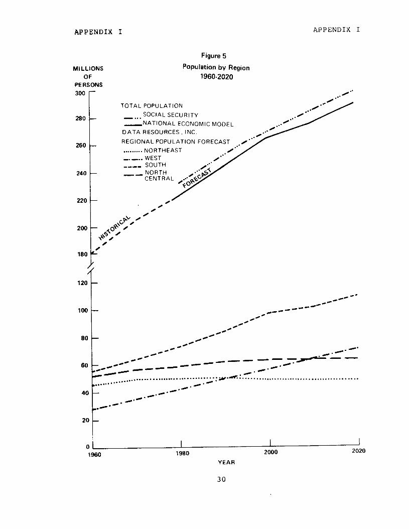
Fiyure 5 shows the total U.S. population and the population by census region as obtained from the national economic model and a forecast by the Social Security Adminis- tration. The Social Security forecast is slightly higher than the national economic model forecast. Both forecasts of total U.S. population show a slowdown in the rate of population growth. Regional population growth as forecast by the DRI national economic model provides for slow growth in the north-central region, substantial growth in the western and southern regions, and a modest decline in the northeast region.

The other important factor is the forecast of the potential output of the economy. The DRI model's forecasts of inflation and real GNP growth rates are similar to Social Security Administration estimates of these variables. The DRI model forecasts a long-term real GNP growth rate of 2.5 percent and a long-term inflation rate of 4.5 percent L/; the Social Security Administration 2/ forecasts 3.0 percent and 4.0 percent, respectively, for real GNP and inflation. Recent, persistent economic events have forced the choice of a higher inflation rate. An inflation rate of roughly 7 percent was chosen as representative of recent trends.

The following sections present the projections of State and local government employment and salary growth along with a detailed description of the employment and salary model's structure and assumptions.

L/The national economic model uses the personal consumption deflator while Social Security uses CPI. The personal consumption deflator is a broad-based inflation index used to deflate total personal consumption expenditures for all consumers, not just inflation's impact on urban consumers as measured by the Consumer Price Index (CPI). For a 25- year forecast period (1979-2003), the average annual rate of increase in the personal consumption deflator is 0.4 percent below the respective forecast of the Consumer Price Index - All Urban Consumers.

z/1978 Annual Report of the Board of Trustees, Old-Age and Survivors Insurance and Disability Insurance, p. 24. The economic assumptions for the Alternative II forecast for the year 1978-1981 are similar to the economic assumptions underlying the President's FY 1979 Budget.

29


Figure 5

Population by Region

1960-2020 MILLIONS

OF PERSONS 300

TOTAL POPULATION

SOCIAL SECURITY D . . . ,-NATIONAL ECCNOMIC MODEL

DATA RESOURCES, INC.

REGIONAL POPU

. . . . . . . . . NORTHEAST -.-.. WEST -me- SOUTH

NORTH - - CENTRAL

80

60

!

01 I I

1960 1980 2000 2020

YEAR

30


THE EMPLOYMENT MODEL

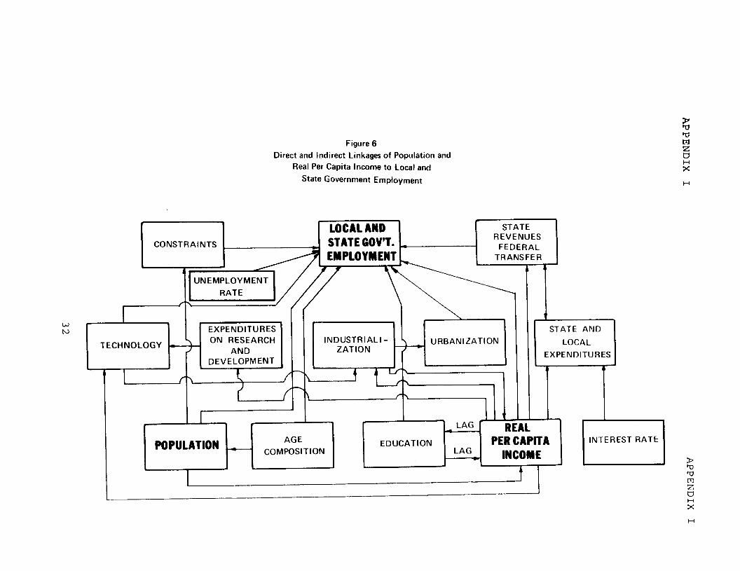
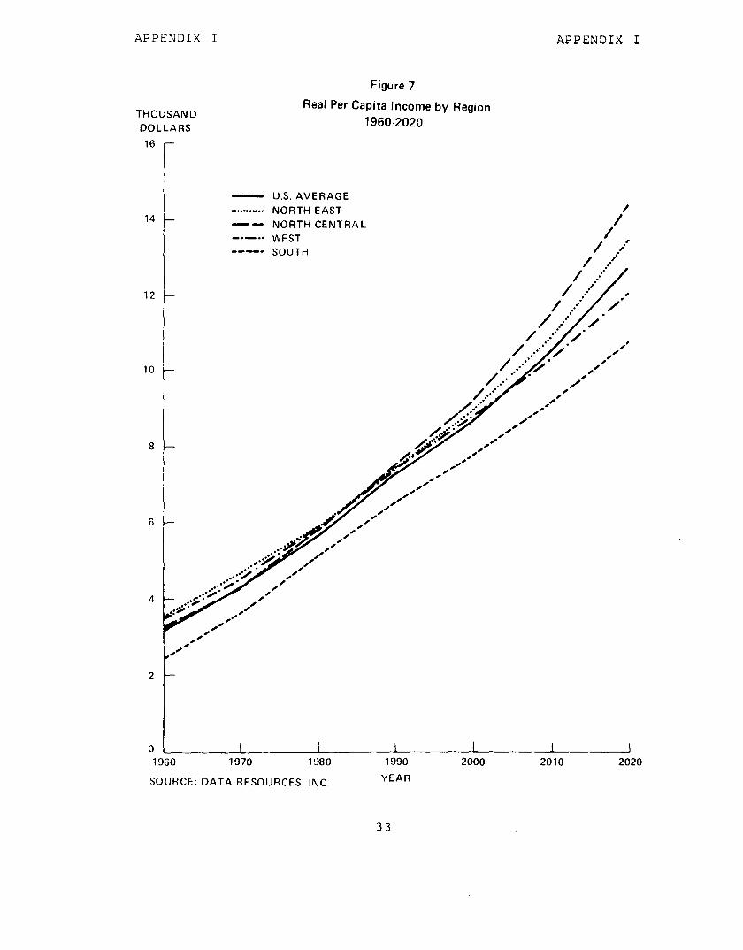
The employment model projects six employment categories within each region--police, firemen, local teachers, State teachers, all other local employees, and all other State employees. Projections in each category of employment were made using econometric techniques that accounted for the impact of population and real per capita income on the demand for services from State and local government employees. Real per capita income is highly correlated with a number of other factors which affect local and State government employment, such as urbanization, education, and real per capita Federal Government transfers to State governments. (See figure 6.) These others are not included since they would measure the same effect as measured by real per capita income. Figure 7 shows historical and forecast real per capita income as obtained from the national economic model.

Constraining the employment projections

As the population in a region increases, the demand for additional services from each functional State and local government employment category increases. Rising real per capita income increases the standard of living, which, in turn, increases the demand for police and fire protection, higher education and other State and local government services. In our opinion there is a limit to the demand for services even if real per capita income increases. By constraining the level of employment per million population in the employment model, the effect of increasing real per capita income on the demand for State and local government services is limited. We analyzed historical data on the growth of State and local government employment to establish our employment constraints.

Table 10 shows historical State and local government employment per million population by census region. These figures can be viewed as showing a real income effect on employment of providing a given level of State and local government service. For example, increased real per capita income was associated with an increase in police employment in the northeast region from 2,098 per million in 1957 to 2,956 per million in 1977. This is much higher than in the other regions although other regions have grown faster in the last 20 years. The higher demand for police protection in the northeast compared to other regions can be attributed to higher levels of real per capita income, urbanization and education. Similar regional growth patterns can be seen for firemen.

31

r

Figure 6 Direct and Indirect Linkages of Population and

Real Per Capita Income to Local and

State Government Employment

r LOCAL AND STATE

CONSTRAINTS , _ STATEGOV’T. c REVENUES FEDERAL ----_ -__---__-

EMPLOYMENT 1 TRANSFER

W N

r-

TECHNOLOGY

STATE AND

LOCAL EXPENDITURES

‘7 I . I I 1 LAG REAL

EDUCATION PER CAPITA LAG

-w INCOME

t I

INTEREST RATE I


THOUSAND

DOLLARS

16

8

Figure 7

Real Per Capita Income by Region 1960-2020

- U.S. AVERAGE -..-..... NORTH EAST

- - NORTH CENTRAL

-*-a* WEST ---- SOUTH

SOURCE: DATA RESOURCES, INC. YEAR


Year __~- Northeast -- North-Central South West

POLICE

1957 2,098 1,444 1,261 1,600 1967 2,437 1,762 1,675 2,005 1977 2,956 2,384 2,395 2,777

FIREMEN

1957 1,084 685 569 879 1967 1,121 852 770 918 1977 1,144 876 979 1,135

LOCAL TEACHERS

1957 9,382 10,657 10,374 12,009 1967 15,373 15,562 15,992 17,370 1977 17,980 18,963 19,614 18,900

STATE TEACHERS

1957 688 1,773 2,580 2,261 1967 1,695 3,461 3,292 4,303 1977 2,494 4,890 5,322 5,741

LOCAL ALL OTHERS

1957 9,817 8,214 6,767 9,638 1967 10,936 9,768 9,143 11,199 1977 13,448 11,845 12,227 14,694

STATE ALL OTHERS

1957 5,769 4,278 5,182 5,320 1967 6,984 5,488 6,723 6,804 1977 8,845 6,961 9,487 8,249

Table 10

Em- One Million Population -. by Region-in Each Functional

Categor y of Local and State ---- Government for 1957, 1967, and 1977 --

The growth in real per capita income from 1957 to 1977 in all the regions has created a substantial demand for higher education, as evidenced by a dramatic increase in local and State government employment in education in all the regions. Similarly, increased real per capita income and the parall&:!

34

APPE;IDIX I APPENDIX I

growth in urbanization and education in all the regions has caused substantial increases in the demand for various tradi- tional services. It has also created a demand for new types of services in all the regions in the last 20 years. This is substantiated by the increase in all other local and State government employment.

Increases in regional employment per million population have been substantial. This trend is not forecast to continue at the historical rate. The employment model constrains employment per million not to exceed the limits shown in table

Table 11 -___-

by Functional- ___-__

Functional cateqory

Police

Firemen

Employment per million peom

3,498

1,210

Local teachers 26,871

State teachers 7,250

All other local 17,464

All other State 11,805

Million -

Number of persons served by one -job

286

826

37

138

57

85

Statistical estimation

Employment is projected taking into account both the population effect and a constrained real income effect. The employment model traces the real income effect on each category of State and local government employment in each reyion when population is kept constant. By limiting the amount of employment per million population, an upper limit to the income effect was incorporated into the model. The model is

E 0 Pt = e

(B. + B1 /Xt )

E Where p is the employment per million people in the year t and Xt is the real per capita income in the year t. Bc, and Bl are the parameters to be estimated. E$J is positive and 01 is negative. The functional upper limit for E is $0;

F

35


judgmental limits were added as discussed in the ..revious section. The model was estimated in logaritnmic fdrm and adjusted for serial correlation for the six functional State and local government employment categories and the four Cen- sus regions.

Table 12 shows the regression coeffficient, % 2

and rho values for the regression equations fitted for all the functional categories of employment in all the regions. All the coefficients are s atistically siynificant at the five percent level. -f The R values are generally hiyher than 0.90, indicating that the real per capita income serves to explain more than 90 percent of the variation of the ratio of employment to population in all functional categor-Les in all regions except two cases duriny the past 20 years.

THE SALARY MODEL

Real annual salaries for State and local government employees correlated with real per capita income in each region. Hence, real per capita income in each region was used as a proxy for all the independent variables which can explain the variation in the real annual average salary:

Zt = e’% + BL4)

where: zt = real average annual salary

xt = real per capita income.

Bo and i31 are the parameters to be estimated. The equations were adjusted for serial correlation. Using the reciprocal of real per capita income in the equation provides estimates of real average annual salary increasing at a decreasing rate. The nominal average annual salary is estimated by inflatiny the estimated real average annual salary by the estimated cost-of-living adjustment.

Statistical estimation

Table 13 shows the regression coefficients, R 2

and rho values for the regression equations fitted in all the functional categories of employment in all the regions. The t- statistic values are not specifically given in the table because all the coefficients are statistically different fro:;i zero even at the 1 percent level of significance. In most cases, the %? values are higher than 0.90 indicating that the real per capita income in the reciprocal form explains more than 90 percent of the variation in real annual avertii;. salary in most functional categories in most of the regi!::.: during the past 20 years.

36


Table 12 -_--_ L

The Regressio - -- Values in the Functions Fitted in

Ali-%Functional Cateuories of Employment in all Regions -

Region

Northeast North Central South West



Northeast 11.0924 -0.388012 0.9691 0.479518 North Central 10.7469 -0.361185 0.9591 0.131219 South 10.5037 -0.359309 0.9854 0.517653 West 10.5314 -0.304363 0.9591 0.576608



Constant Term _ Coefficient

POLICE --___-

9.02753 -0.514545 8.35954 -0.2471)47 8.43121 -0.304263 9.18427 -0.487819

FIREMEN -____

6.92650 -0.606711 6.68000 -0.181161 7.44157 -0.424566 8.76935 -0.815335

STATE TEACHERS

9.42259 -0.186327 9.89154 -0.420489 9.45790 -0.401093

10.4506 -0.609410

LOCAL TEACHERS

ALL OTHER STATE EMPLOYMENT

2 R - rho

0.9557 0.769005 0.9671 0.822922 0.9816 0.824848 0.9727 0.725204

0.6534 0.568054 0.4672 0.024509 0.9714 0.729988 0.9104 0.5083Y7

0.9877 0.150395 0.9718 0.410339 0.9623 0.783857 0.9718 0.699416

9.91185 -0.351661 0.9735 9.50252 -0.190730 0.9610 9.74615 -0.414401 3.9786 9.56413 -0.253079 0.9198

ALL OTHER LOCAL EMPLOYMENT

0.708181 0.408203 0.874219 0.500326

37


Table 13 --- - 2

The Regression Coefficients, R and rho Values in the _-- Functions Fitted in all the Functional Forms in all Kegions -- for Real Average Annual Salaries -

Region Constant

term Coefficient --

POLICE

2 z - rho --

Northeast 10.4465 -5.49074 North Central 9.96977 -3.57118 South 9.58124 -2.23339 West 10.1709 -4.00828

FIREMEN

0.9460 -0.12388 0.9632 0.579616 0.9854 0.310168 0.9644 0.709396


LOCAL TEACHERS

0.9790 0.29997 0.9570 0.604772 0.9887 0.59363 0.9598 0.71527


STATE TEACHERS

0.9386 0.56105 0.9135 0.53234 0.9276 0.748328 0.9548 0.884518


ALL OTHER STATE

0.9298 0.511627 0.8908 0.575996 0.9525 0.824976 0.8293 0.531574

Northeast 10.00230 -4.47651 North Central 9.83174 -3.59774 South 9.52789 -2.47126 West a/ 10.0543 -3.91404 -

ALL OTHER LOCAL

0.9780 0.77894 0.9570 0.60509 0.9863 0.55148 0.9344 OLS


a/The equation was estimated using ordinary least squares. -

38

APPENDIX II

MODEL TO FORECAST BENEFIT PAYMENTS ---.-

UPENUIX II

In 1975, the Pension Task Force and the GAO undertook a study of State and local government retirement systems, as required under Section 3031 of the Employee Retirement Income Security Act of 1974 (ERISA). An integral part of the study was a survey of pension plan membership characteristics and requirements, contributions, vesting, benefits, portability, and financing. The survey generated a large data base, with information representing 6,630 State and local pension plans.

The Task Force data base was used as the starting point to project benefit payout. To that extent, the data merit a discussion because of the picture they present of the overall characteristics of State and local government retirement systems in 1975. Table 14 shows the membership in all State and local plans, in all large plans (those with 1,000 or more active employees), and in all large defined benefit plans. Large plans, although only 6 percent of all plans, represent about 94 percent of the total active membership, while the 297 defined benefit plans contain over three-fourths of the total membership.

In 1975 active membership in large defined plans was 8.1 million, of whom 70 percent were also covered by Social Security. Social Security benefits were not included in any of our projections because they were not integrated with the State and local plans to any appreciable degree. In addition, there were 1.6 million retirees, over three-fourths of whom were retired because of age and service.

Most of the 82 large plans that are not defined benefit plans have features of both defined contribution and defined benefit plans and are referred to as "combination" plans. As might be expected, the large State and local government

Table 14 ___-

Membership in State and Local Retirement Systems in 1975 -___

Percent- Nurnber of Number Membership (thousands) aye of Members

of plans Active Inactive Total Total --- - ____ per Plan

All 6,630 10,387 2,347 12,734 100.0 1,920 All large 379 9,859 2,112 11,971 93.9 21,600 Larye

defined benefit 279 8,070 1,612 9,682 76.0 32,600

39

APPENDIX II APPENDIX 11

retirement systems have a financial impact commensurate with the size of their membership.

Table 15 shows that large defined benefit plans account for about three-fourths of the total of all State and local government plans in key financial areas, while all large plans are over 90 percent of the total. We restricted our detailed analysis to the large defined benefit plans in an effort to ensure a level of homogeneity that would make projections practical. The intention was to use the information from the Task Force survey to build prototypes of State and local government plans and then project pension costs for State and local government retirement systems as a whole. Defined benefit plans exhibited sufficient similarities in provisions, experience, and funding to allow the construction of "typical" plans.

Most of the active members were in plans whose benefit formulas were a simple percentage (rate) of final compensation times years of service. Post-retirement cost-of-living adjustments took various forms, including ad hoc increases, automatic increases with the cost of living (but subject to

Table 15

General Financial Characteristics (in billions of dollars)

Assets

Investment Income

Benefit Payout

Employer Contri- butions

Employee Mandatory Contribu- tions

Payroll

Percent Percent Large Defined of all All Large of all All Benefit Plans Plans Plans Plans Plans

$80.7 75 $101.5 94 $108.3

4.3 72 5.5 93 5.9

5.8 73 7.5 95 7.9

7.4 73 9.3 92 10.1

4.1 77 5.1 95 5.4

74.2 76 92.6 95 97.5

40

APPENDIX II APPENDIX II

a limit), and constant percentage increases. The Task Force's limited survey of 23 very large retirement systems (with total 1975-76 active membership of 4.5 million) revealed that post- retirement adjustments averayed, from 1969 to 1978, about one-half the increase in the Consumer Price Index. At least 87 percent of the large defined benefit plans featured mandatory employee contributions, usually at a simple percentage of salary, and 92 percent of the employees were in plans with some advanced funding.

MODEL TO FORECAST BENEFIT PAYOUT

The large defined benefit plans were divided into two groups --teachers' plans and other plans. A review of the responses to the Task Force survey and other actuarial material led to the conclusion that these two types of plans were too dissimilar to combine. For example, the teachers had in general more yenerous benefits, higher salaries, a different age and sex distribution, and higher withdrawal rates. Because each of these characteristics weighs heavily in a benefit projection, we developed two separate prototypical plans whose 1975 membership, total benefits, and average annual salaries are shown in table 1, page 5. Each prototype was designed to conform initially to these characteristics. In addition, we used the Task Force data to determine the number of years on which to base "final compensation" and to construct the two prototypical benefit formulas.

Other data sources were used in those areas that the Task Force survey had not covered. The age and sex distributions of the active populations were based upon information in the Census Bureau's "Current Population Survey" (January 1978) . For age and benefit distributions of the 1975 retirees, data were aggregated from actuarial valuations of several large State, local and teachers' retirement systems. These valuations also supplied us some data on retirement ages, entry ages, withdrawal and disability rates, and salary scales. Post-retirement cost-of-living adjustments were set at half the future increases in the cost of living. We used the Unisex Pension 1984 Table, adjusted for varying male- female ratios and future improvements in mortality.

PROJECTING BENEFITS

Within each prototype, benefits were projected for three groups: persons retired in 1975, active employees in 1975, and new entrants after 1975. Projections through the year 2020 of the growth both in teachers' and in other State and local governments' work forces were incorporated into the model and served to predetermine the number of new entrants needed each year in the future.

41


The 1975 retirees were assigned an initial age and benefit distribution and then "aged" using the assumed mortality rates. A projection through 2020 of the cost Of living was used in computiny the remaining retirees' post-retirement Cost-of-liviny adjustments. i/

An age distribution from the BLS "Current Population Survey" was imposed on the 1975 active employees in each prototype. The total payroll (average salary times number of employees) was distributed initially among the age groups using a merit scale to reflect a typical worker's career salary progression, neglecting inflation. The career average annual merit increase was 1 percent for State and local government employees and l-1/2 percent for teachers, with accelerated increases in the early years. At each year of the projection, salary growth forecasts were applied across the board to the total payroll.

Those actives who "survived" to retirement were accorded a benefit using the average benefit formulas constructed from the Task Force data. Retirement ages were spread uniformly over a lo-year period, with the median age determined by a review of actuarial valuations and plan provisions.

Entry ages were set at 30 and 34 for the teachers' and the State and local prototypes, respectively, and represent the average entry age for a typical retiree. The benefit formulas, entry ayes, and retirement ayes result in an average replacement ratio (that is, percentage of final compensation) of 52 percent for teachers and 50 percent for other State and local retirees. Final compensation in both prototypes was the average of the last 4 years of salary.

Augmenting the benefits

The average benefit formulas as computed could be applied directly only to those employees retiring because of age and service. Furthermore, the benefits so generated were confined to the modeled population--that is, large defined benefit teachers' and other State and local pension plans. To obtain projection for all 6,630 plans, the prototypical benefits had to be augmented first for ancillary benefits and second for all those plans outside the modeled population. Four augmen- tations were made in each year of the projections.

The prototypes dealt exclusively with members who retired because of age and service. Survivor benefits, disability

L/See p. 29, app. I.

42


benefits, and returns of contribution were not separately calculated. Instead, we augmented the average benefit going to age and service retirees to take into account the payments for these ancillary benefits. The augmentation factors we used were based on the Bureau of the Census data for 1974 to 1977.

Among the 297 large defined benefit plans were 46 plans for police and firemen. Although 15 percent of the plans, they represented just 3 percent of the active employees and as such were considered too insignificant to merit their own prototype. To take these plans into account, total benefits were increased proportionately.

The combination and defined contribution plans were found to be similar to the large defined benefit plans in key financial areas. Differences in average benefit and average salary for 1975 were recognized before augmenting the prototypes' benefits by the ratio of total actives in all 379 plans to total actives in the 297 defined benefit plans. L/

The 6,251 small plans accounted in 1975 for less than 5 percent of the active membership in State and local government pension plans. The model's total benefit payments were increased proportionately to take into account these additional plans and thereby extend the model to the known 1975 universe of State and local government retirement systems. Table 16 summarizes the assumptions used.

About 42 percent of State and local government systems of all types were funded on a nonactuarial basis. Moreover, many claiming to use an actuarial basis were not using the "dynamic normal cost" approach 2/ recommended by GAO for all Federal plans. The Task Force went on to estimate that only 20 to 25 percent of all State and local government pension plans would meet ERISA's minimum funding standards.

l/See table 14.

z/This approach takes into account future cost-of-living increases and general pay hikes.

43


Table 16

Base Case Projection Assumptions

* at retirement Median age 60 for teachers, with lo-year spreading Median aye 62 for State and local employees, with lo-year spreadiny

Entry age

Rates of mortalitv

Rates of withdrawal (original actives)

(New entrants)

Rates of disability A!35 Rate per thousand

Benefit formulas Teachers

30 for teachers 34 for State and local employees

Unisex Pension-1984 Table, with one-year setback for every 17 years of projection

Sample annual rates of termination are as follows:

%F Teachers State & local

25 15.9% 16.0% 30 5.7% 11.4% 35 2.6% 7.4% 40 1.2% 5.1% 45 0.6% 3.9% 50 0.3% 3.0%

35 5.4% 13.9% 40 1.1% 5.3% 45 0.4% 3.2% 50 0.2% 1.6% 55 0.1% 1.0%

25 0.600 30 0.672 35 0.768 40 0.920 45 1.926 50 1.920

1.85% x years of service x final compensation.

State & local 1.78% x years of service x final compensation.

44


Final compensation ~-

Average Service at retirement

-

Replacement ratios --

Ancillary benefits

Table 16--Cont.

Averaye of last 4 years of salary.

28 years

Teachers -___ 51.8%

State & local 49.7% P-P

Teachers Projected as a constan?! 7.6% of total payout.

State & local Projected as a constant 16.4% of total payout.

Withdrawal payments Teachers (Return of contributions)

Projected at 9.5% of total payout.

State & local Projected at 15.2% of total payout.

45

Single copies of GAO reports are available free of charge. Requests (except by Members of Congress) for additional quantities should be accompanied by payment of $1.00 per copy *

Requests for single copies (without charge) should be sent to:

U.S. General Accounting Office Distribution Section, Room 1518 441 G Street, NW. Washington, DC 20548

Requests for multiple copies should be sent with checks or money orders to:

U.S. General Accounting Office Distribution Section P.O. Box 1020 Washington, DC 20013

Checks or money orders should be made payable to the U.S. General Accounting Of- fice. NOTE: Stamps or Superintendent of Documents coupons will not be accepted.

PLEASE DO NOT SEND CASH

To expedite filling your order, use the report number and date in the lower right corner of the front cover.

GAO reports are now available on micro-

AN EQUAL OPPORTUNITY EMPLOYER

UNITED STATES GENERAL ACCOUNTINGOFFTCE

WASHINGTON, D.C. 2098

OPflCIAL BUSlNtSS PENALTY FOR PRIVATE US&S300

POSTAGE AND ?ICS PAID - U. ,. OCWIRAL ACCOUNTING OC?lCC

THIRD CLASS