Embed Size (px)
Citation preview
Bringing Expertise Into Focus
Packet Network Timing Measurements,
Metrics, and Analysis
ITSF 2010
Lee Cosart

Presentation Outline
Introduction Types of measurements:
1. Synchronization “TIE”
2. Packet “PDV”
3. Packet “Load”
Measurement equipment overview
Synchronization and Packet Analysis TIE and PDV based metrics
Packet selection processes and methods
Frequency transport metrics
Time transport metrics
Network Measurements Lab/production packet network measurements
Linking packet delay metrics to sync performance
Load Probe Load probe measurement theory
“Load” and “PDV” measurement relationship
Network load probe measurements2
“TIE” vs. “PDV”
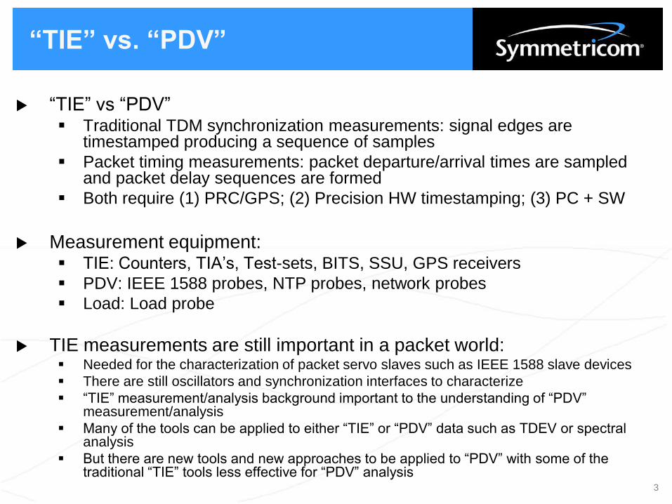
“TIE” vs “PDV” Traditional TDM synchronization measurements: signal edges are
timestamped producing a sequence of samples
Packet timing measurements: packet departure/arrival times are sampled and packet delay sequences are formed
Both require (1) PRC/GPS; (2) Precision HW timestamping; (3) PC + SW
Measurement equipment: TIE: Counters, TIA’s, Test-sets, BITS, SSU, GPS receivers
PDV: IEEE 1588 probes, NTP probes, network probes
Load: Load probe
TIE measurements are still important in a packet world: Needed for the characterization of packet servo slaves such as IEEE 1588 slave devices
There are still oscillators and synchronization interfaces to characterize
“TIE” measurement/analysis background important to the understanding of “PDV” measurement/analysis
Many of the tools can be applied to either “TIE” or “PDV” data such as TDEV or spectral analysis
But there are new tools and new approaches to be applied to “PDV” with some of the traditional “TIE” tools less effective for “PDV” analysis
3
“TIE” vs. “PDV”
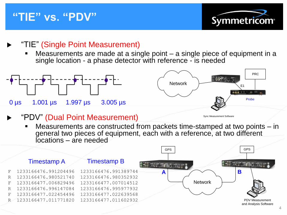
“TIE” (Single Point Measurement) Measurements are made at a single point – a single piece of equipment in a
single location - a phase detector with reference - is needed
“PDV” (Dual Point Measurement) Measurements are constructed from packets time-stamped at two points – in
general two pieces of equipment, each with a reference, at two different locations – are needed
0 µs 1.001 µs 1.997 µs 3.005 µs
GPS
PDV Measurement
and Analysis Software
Network
GPS
F 1233166476.991204496 1233166476.991389744
R 1233166476.980521740 1233166476.980352932
F 1233166477.006829496 1233166477.007014512
R 1233166476.996147084 1233166476.995977932
F 1233166477.022454496 1233166477.022639568
R 1233166477.011771820 1233166477.011602932
A B
Timestamp A Timestamp B
Network
PRC
Probe
E1
Sync Measurement Software
4

“PDV” Measurement Setup Options
“PDV” Ideal setup - two packet timestampers with GPS reference so absolute
latency can be measured as well as PDV over small to large areas
Alternative setup (lab) – frequency (or GPS) locked single shelf with two packet timestampers
Alternative setup (field) – frequency locked packet timestampers – PDV but not latency can be measured
PDV Measurement
Software
GPS
1588 GM
Hub
PDV Measurement
Software
Analysis Software Network
1588 Slave
GPS
Probe
GPS
PDV Measurement
and Analysis SoftwareNetwork
1588 GMProbe
GPS
Active Probe(1) No Hub or Ethernet Tap Needed
(2) No IEEE 1588 Slave Needed
(3) Collection at Probe Node Only
Passive Probe(1) Hub or Ethernet Tap
(2) IEEE 1588 Slave
(3) Collection at Both Nodes
5

“TIE” and “PDV” and “Load”
In most packet network measurement setups, both “TIE” and “PDV”
are measured at the same time
GPS
PDV
Measurement
Software
Network
GPS
GPS
1588
Grandmaster
1588 Probe
Probe
E1 or
T1
IP
IP
IP
1588 Slave
Sync Measurement
Software
IPLoad Probe
later
Load
Measurement
Software0.0 s
0.0 s
1.5 ms
1.03
days
0.0
days
1.5 ms
2.0 hours/div
Symmetricom TimeMonitor Analyzer; Network Emulator; 2009/07/21; 23:33:10
Symmetricom TimeMonitor Analyzer; Live Network; 2009/03/04; 17:06:25
Live
Network
Network
Emulator
Network
Emulator
6
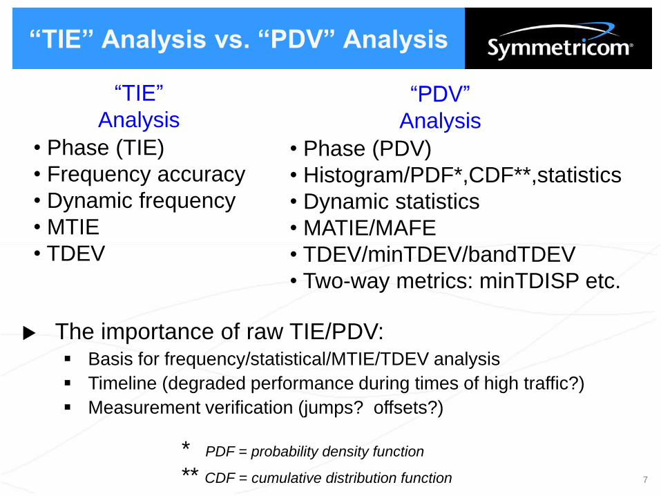
“TIE” Analysis vs. “PDV” Analysis
“TIE”
Analysis“PDV”
Analysis
* PDF = probability density function
** CDF = cumulative distribution function
• Phase (TIE)
• Frequency accuracy
• Dynamic frequency
• MTIE
• TDEV
• Phase (PDV)
• Histogram/PDF*,CDF**,statistics
• Dynamic statistics
• MATIE/MAFE
• TDEV/minTDEV/bandTDEV
• Two-way metrics: minTDISP etc.
The importance of raw TIE/PDV: Basis for frequency/statistical/MTIE/TDEV analysis
Timeline (degraded performance during times of high traffic?)
Measurement verification (jumps? offsets?)
7

Analysis from Phase: Frequency
Point-by-point
Sliding Window Averaging
Segmented LSF
1.5 E-9
1.2 E-11
1.2 E-11
-8.97·10-14 Frequency Accuracy
dt
d slope/linear: frequency offset
curvature/quadratic: frequency drift
8
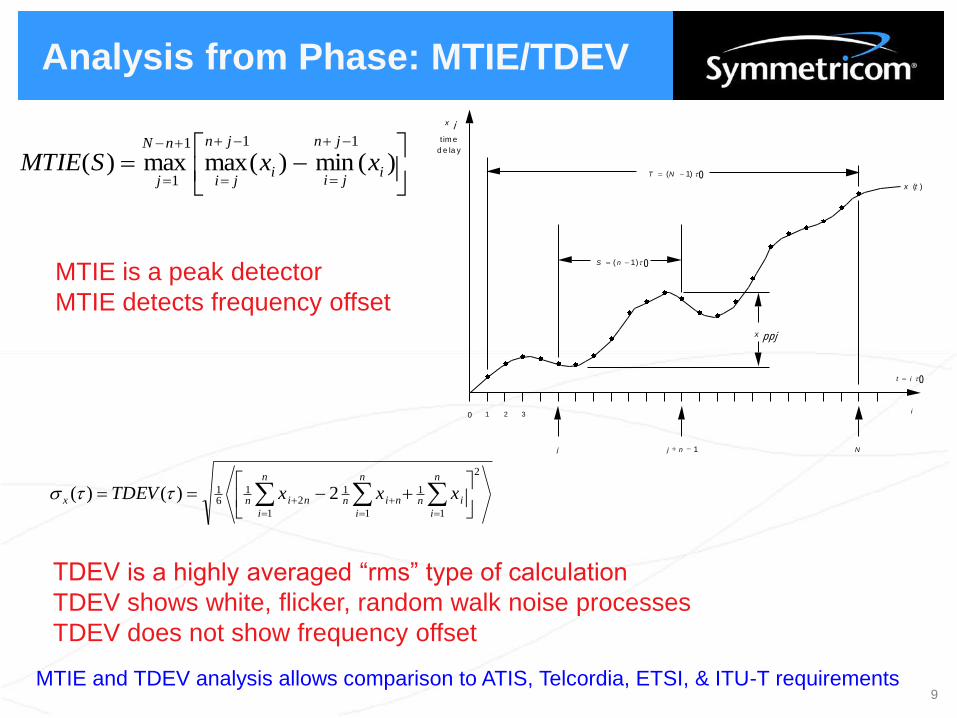
Analysis from Phase: MTIE/TDEV
0 1 2 3
t im e
d e la y
j j n 1 N
i
x ( t )
x ppj
x i
S ( n 1 ) 0
T ( N 1 ) 0
t i 0
)(min)(maxmax)(
111
1i
jn
jii
jn
ji
nN
jxxSMTIE
MTIE is a peak detector
MTIE detects frequency offset
2
1
1
1
1
1
21
61 2)()(
n
i
in
n
i
nin
n
i
ninx xxxTDEV
TDEV is a highly averaged “rms” type of calculation
TDEV shows white, flicker, random walk noise processes
TDEV does not show frequency offset
MTIE and TDEV analysis allows comparison to ATIS, Telcordia, ETSI, & ITU-T requirements9

Stability metrics for PDV
Packet Selection Processes1) Pre-processed: packet selection step prior to calculation
Example: TDEV(PDVmin) where PDVmin is a new sequence based on minimum searches on the original PDV sequence
2) Integrated: packet selection integrated into calculation
Example: minTDEV(PDV)
Packet Selection Methods
Minimum:
Percentile:
Band:
Cluster:
1minmin nijiforxix j
b
aj
ijmmeanband xix 1_
b
j
ijmmeanpct xix0
1_
)1(
0
)1(
00
),(
,)(
)(K
i
K
i
P
in
ininKw
nx
otherwise
ninKw for in
0
)()(1,
10

Packet Delay Sequence
Packet Delay Sequence
R,00162; 1223305830.478035356; 1223305830.474701511
F,00167; 1223305830.488078908; 1223305830.490552012
R,00163; 1223305830.492882604; 1223305830.489969511
F,00168; 1223305830.503473436; 1223305830.505803244
R,00164; 1223305830.508647148; 1223305830.505821031
F,00169; 1223305830.519029300; 1223305830.521302172
R,00165; 1223305830.524413852; 1223305830.521446071
F,00170; 1223305830.534542972; 1223305830.536801164
R,00166; 1223305830.540181132; 1223305830.537115991
F,00171; 1223305830.550229692; 1223305830.552551628
#Start: 2009/10/06 15:10:30
0.0000, 2.473E-3
0.0155, 2.330E-3
0.0312, 2.273E-3
0.0467, 2.258E-3
0.0623, 2.322E-3
#Start: 2009/10/06 15:10:30
0.0000, 3.334E-3
0.0153, 2.913E-3
0.0311, 2.826E-3
0.0467, 2.968E-3
0.0624, 3.065E-3
Forward Reverse
Packet
Timestamps
11
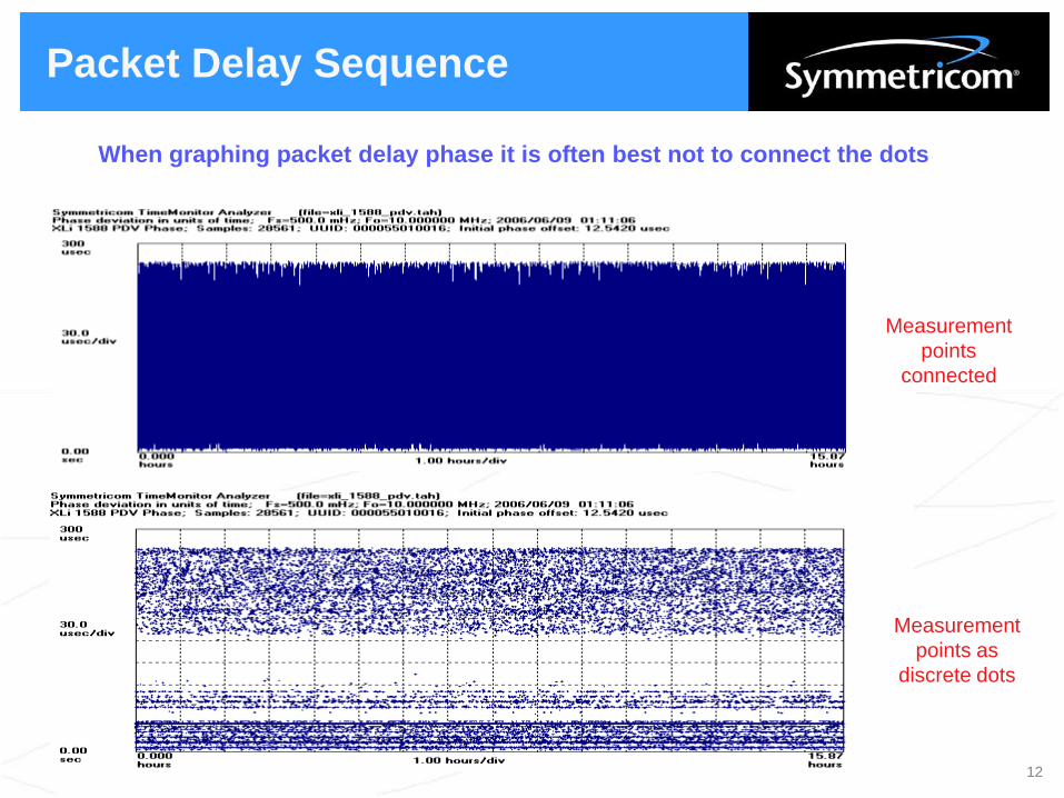
Packet Delay Sequence
When graphing packet delay phase it is often best not to connect the dots
Measurement
points
connected
Measurement
points as
discrete dots
12
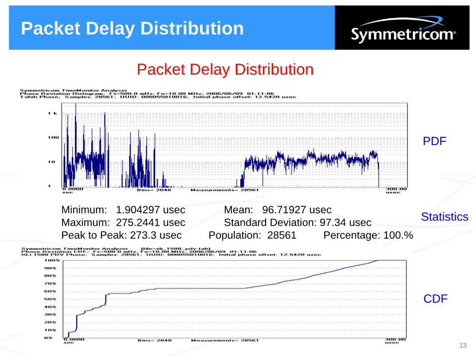
Packet Delay Distribution
Packet Delay Distribution
Minimum: 1.904297 usec Mean: 96.71927 usec
Maximum: 275.2441 usec Standard Deviation: 97.34 usec
Peak to Peak: 273.3 usec Population: 28561 Percentage: 100.%
13
CDF
Statistics

Tracked Packet Delay Statistics
Raw packet delay appears
relatively static over time
Mean vs. time shows cyclical
ramping more clearly
Standard deviation vs. time shows
a quick ramp up to a flat peak
14
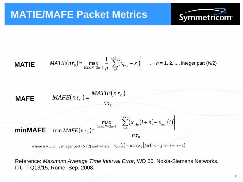
MATIE/MAFE Packet Metrics
MATIE
1
1210
1max
kn
ki
ininNk
xxn
nMATIE , n = 1, 2, ..., integer part (N/2)
0
00
n
nMATIEnMAFE MAFE
Reference: Maximum Average Time Interval Error, WD 60, Nokia-Siemens Networks,
ITU-T Q13/15, Rome, Sep. 2008.
15
0
1
minmin121
0
max
min
n
ixnix
nMAFE
kn
kinNk
minMAFE
where n = 1, 2, ..., integer part (N/2) and where 1minmin nijiforxix j
.
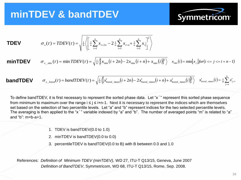
minTDEV & bandTDEV
2
1
1
1
1
1
21
61 2)()(
n
i
in
n
i
nin
n
i
ninx xxxTDEV
2minminmin61
min_ 22)(min)( ixnixnixTDEVx
2___61
_ 22)()( ixnixnixbandTDEV meanbandmeanbandmeanbandbandx
TDEV
minTDEV
bandTDEV
To define bandTDEV, it is first necessary to represent the sorted phase data. Let “x´” represent this sorted phase sequence
from minimum to maximum over the range i ≤ j ≤ i+n-1. Next it is necessary to represent the indices which are themselves
set based on the selection of two percentile levels. Let “a” and “b” represent indices for the two selected percentile levels. The averaging is then applied to the “x´” variable indexed by “a” and “b”. The number of averaged points “m” is related to “a”
and “b”: m=b-a+1.
b
aj
ijmmeanband xix 1_
1minmin nijiforxix j
1. TDEV is bandTDEV(0.0 to 1.0)
2. minTDEV is bandTDEV(0.0 to 0.0)
3. percentileTDEV is bandTDEV(0.0 to B) with B between 0.0 and 1.0
References: Definition of Minimum TDEV (minTDEV), WD 27, ITU-T Q13/15, Geneva, June 2007
Definition of BandTDEV, Symmetricom, WD 68, ITU-T Q13/15, Rome, Sep. 2008.
16

TDEV & minTDEV with Traffic
50% 30% 20% 10% 5% 0%
TDEV
minTDEV
Lower levels of noise with the application of a MINIMUM selection algorithm
minTDEV at various traffic levels on a switch (0% to 50%) converge
No load 5%
10%
35%
50%
17
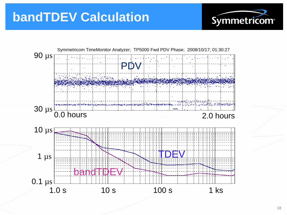
bandTDEV Calculation
0.1 µs
Symmetricom TimeMonitor Analyzer; TP5000 Fwd PDV Phase; 2008/10/17; 01:30:27
PDV
10 µs
0.0 hours 2.0 hours
1.0 s 10 s 100 s 1 ks
TDEV
bandTDEV
90 µs
30 µs
1 µs
18

Metrics: Time Transport
#Start: 2010/03/06 17:15:30
0.0000, 1.47E-6
0.1000, 1.54E-6
0.2000, 1.23E-6
0.3000, 1.40E-6
0.4000, 1.47E-6
0.5000, 1.51E-6
#Start: 2010/03/06 17:15:30
0.0000, 1.11E-6
0.1000, 1.09E-6
0.2000, 1.12E-6
0.3000, 1.13E-6
0.4000, 1.22E-6
0.5000, 1.05E-6
Forward Packet Delay Sequence Reverse Packet Delay Sequence
#Start: 2010/03/06 17:15:30
0.0000, 1.47E-6, 1.11E-6
0.1000, 1.54E-6, 1.09E-6
0.2000, 1.23E-6, 1.12E-6
0.3000, 1.40E-6, 1.13E-6
0.4000, 1.47E-6, 1.22E-6
0.5000, 1.51E-6, 1.05E-6
Two-way
Data Set
Time(s) f(µs) r(µs) f’(µs) r’(µs)
0.0 1.47 1.11
0.1 1.54 1.09 1.23 1.09
0.2 1.23 1.12
0.3 1.40 1.13
0.4 1.47 1.22 1.40 1.05
0.5 1.51 1.05
Minimum Search
Sequence
Constructing f´ and r´from f and r with a 3-
sample time window
19
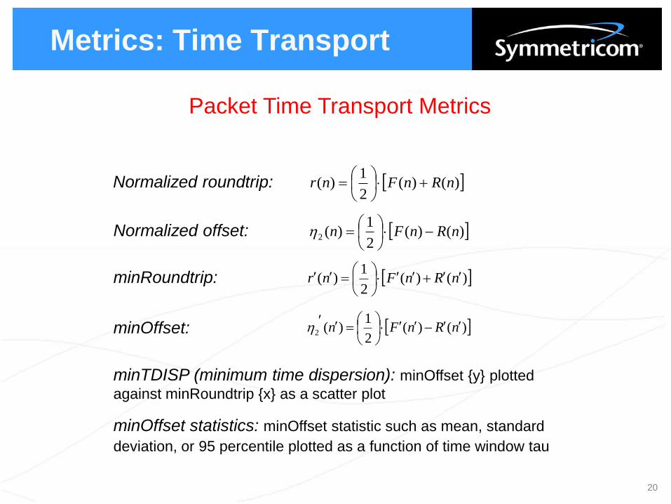
Metrics: Time Transport
Packet Time Transport Metrics
Normalized roundtrip: )()(2
1)( nRnFnr
Normalized offset: )()(2
1)(2 nRnFn
minRoundtrip: )()(2
1)( nRnFnr
minOffset: )()(2
1)(2 nRnFn
minTDISP (minimum time dispersion): minOffset {y} plotted
against minRoundtrip {x} as a scatter plot
minOffset statistics: minOffset statistic such as mean, standard
deviation, or 95 percentile plotted as a function of time window tau
20
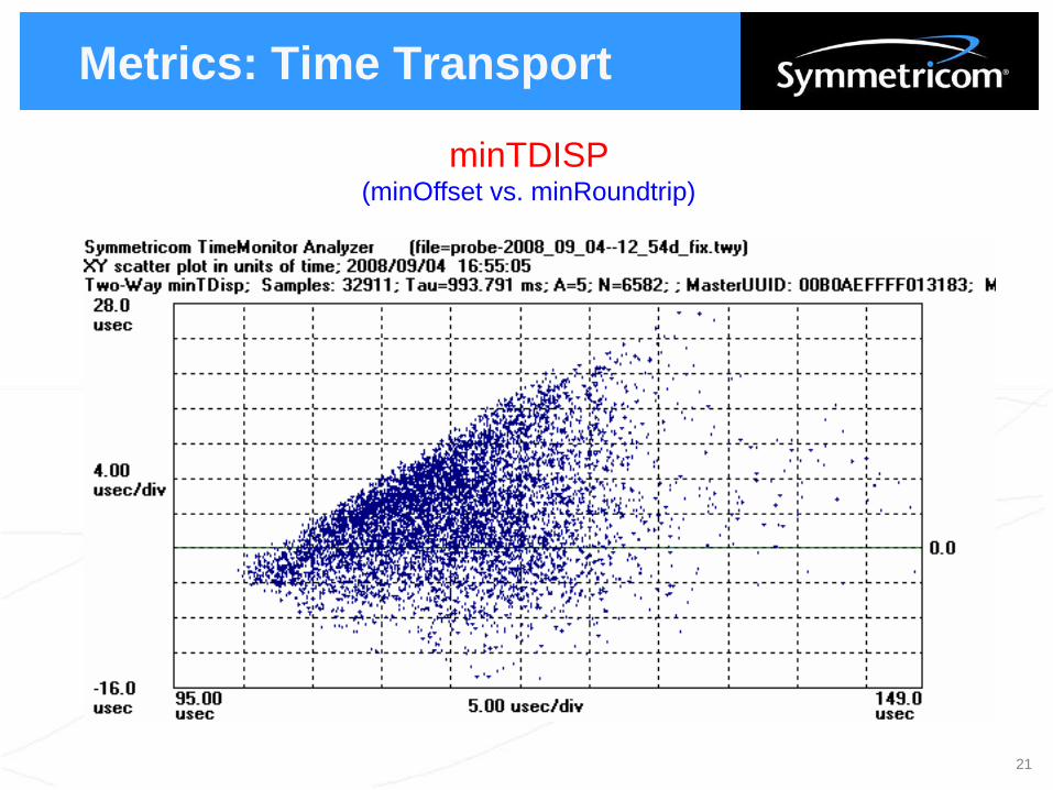
Metrics: Time Transport
minTDISP (minOffset vs. minRoundtrip)
21

Metrics: Time Transport
minOffset Statistics (Two-way minimum offset statistics vs. τ)
22

Case Studies
Asymmetry in Microwave Transport(Ethernet microwave radio packet delay pattern asymmetry )
226 µs
226 µs
244 µs
7.5
minutes
0.0
minutes
244 µs
30 sec/div
Symmetricom TimeMonitor Analyzer; uWave Radio Reverse PDV; 2009/06/23; 23:53:31
Symmetricom TimeMonitor Analyzer; uWave Radio Forward PDV; 2009/06/23; 23:53:31
µWave
Forward
PDV
µWave
Reverse
PDV
2 µs/
div
2 µs/
div
23
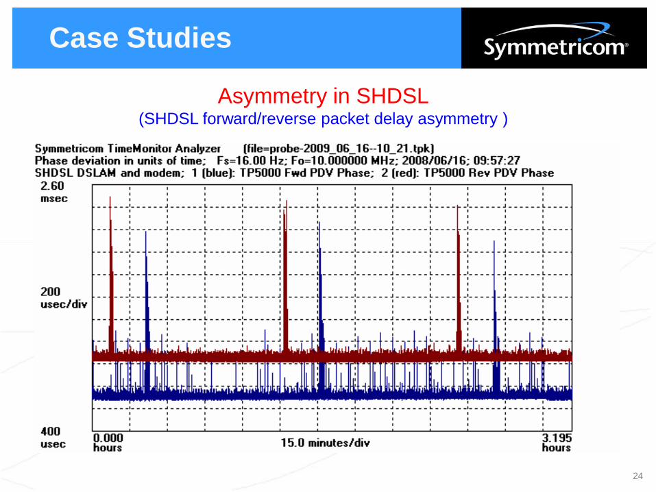
Case Studies
Asymmetry in SHDSL(SHDSL forward/reverse packet delay asymmetry )
24

Case Studies
Asymmetry in Wireless Backhaul(Ethernet wireless backhaul asymmetry and IEEE 1588 slave
1PPS under these asymmetrical network conditions)
-6.0 µs
-1.0 µs
2.0 µs
-2.0µs
Symmetricom TimeMonitor Analyzer; Ethernet Wireless Backhaul; 2009/04/28; 11:37:01
Min
TDISP0.5 µs/
div
1588
Slave
1 PPS
vs.GPS
265.6 µs 270.0 µs
0.5 µs/
div
0.0 hours 22.7 hours
25
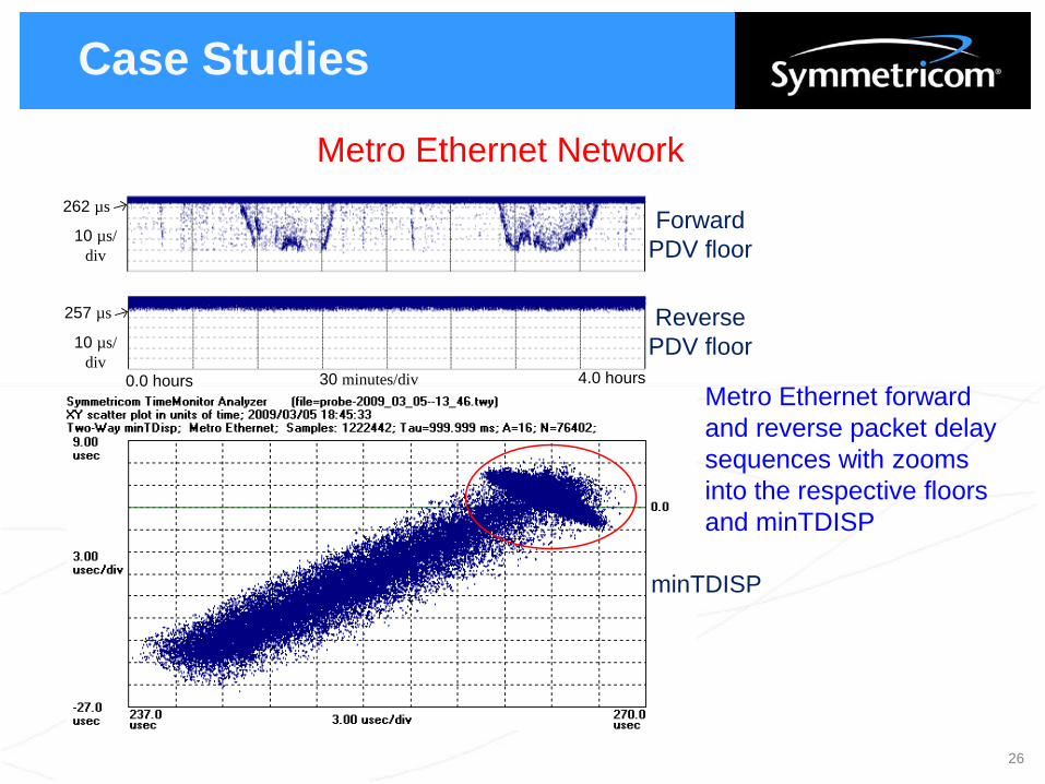
Case Studies
Metro Ethernet Network
10 µs/
div
30 minutes/div
10 µs/
div
Forward
PDV floor
Reverse
PDV floor
minTDISP
262 µs
257 µs
0.0 hours 4.0 hours
Metro Ethernet forward
and reverse packet delay
sequences with zooms
into the respective floors
and minTDISP
26

Case Studies
National Ethernet Network
National Ethernet forward
and reverse packet delay
sequences with zooms
into the respective floors
and minTDISP
1 µs/
div
4.0 hours/div
2 µs/
div
Forward
PDV floor
4.54 ms
Reverse
PDV floor
4.53 ms
minTDISP
0.0 days 1.63 days
27

Sync in a Packet Network
Measurement setup for measuring PDV and the outputs of four 1588 slaves
Network
1588
Master
PRC
1588
Slave
#1
1588
Slave
#2
GigE GigE
TimeMonitor
Measurement
2.048
MHz
2.048
MHz
2.048
MHz
1588
Slave
#3
1588
Slave
#4
2.048
MHz
2.048
MHz
PDV
Probe
TimeMonitor
PDV
TA7500
28

Sync in a Packet Network
1588 slave performance:
1 PPB offset measured
Packet data analysis:
1PPB offset predicted
Packet measurement
Sync measurement
29
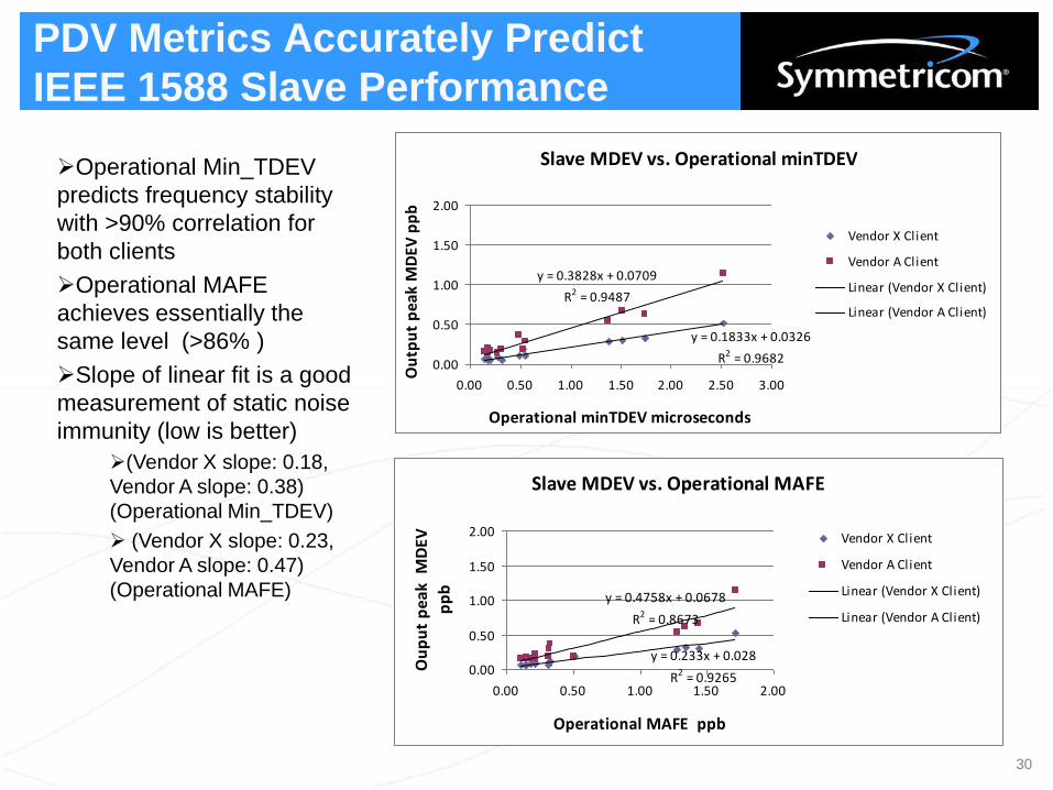
PDV Metrics Accurately Predict
IEEE 1588 Slave Performance
Operational Min_TDEV
predicts frequency stability
with >90% correlation for
both clients
Operational MAFE
achieves essentially the
same level (>86% )
Slope of linear fit is a good
measurement of static noise
immunity (low is better)
(Vendor X slope: 0.18,
Vendor A slope: 0.38)
(Operational Min_TDEV)
(Vendor X slope: 0.23,
Vendor A slope: 0.47)
(Operational MAFE)
Slave MDEV vs. Operational minTDEV
y = 0.1833x + 0.0326
R2 = 0.9682
y = 0.3828x + 0.0709
R2 = 0.9487
0.00
0.50
1.00
1.50
2.00
0.00 0.50 1.00 1.50 2.00 2.50 3.00
Operational minTDEV microseconds O
utp
ut
pea
k M
DEV
pp
b
Vendor X Client
Vendor A Client
Linear (Vendor X Client)
Linear (Vendor A Client)
Slave MDEV vs. Operational MAFE
y = 0.233x + 0.028
R2 = 0.9265
y = 0.4758x + 0.0678
R2 = 0.8673
0.00
0.50
1.00
1.50
2.00
0.00 0.50 1.00 1.50 2.00
Operational MAFE ppb
Ou
pu
t p
ea
k
MD
EV
pp
b
Vendor X Client
Vendor A Client
Linear (Vendor X Client)
Linear (Vendor A Client)
30

“Load” Measurement Probe
Measurement setup for measuring (1) Sync, (2) PDV, and (3) Load
31

Packet Load Probe
Instantaneous packet flow and the derivation of dynamic packet load parameters
Packet Load
(200 msec)
0.1s
Busy
Idle
0.2s
Sample #1 Sample #2
0.0s
Packets 312 1523 95 1167 1030 290 365 297 1245 151 175 1091 1207
Busy (ms) 4 17 1 13 14 4 5 3 13 2 3 12 13
Idle (ms) 5 2 6 7 2 2 9 4 2 7 23 7 4 8 8
Packets Idle Min Idle Max Idle Busy Min Busy Max Busy
Sample #1 5079 39% 2ms 9ms 61% 1ms 17ms
Sample #2 3869 57% 4ms 23ms 43% 2ms 13ms
32

Packet Load Probe
*:008A7484.320859192:AA84008B
0:62123:24617187:75:1525:37883420:11:1584
1:62123:24617187:75:1525:37883420:11:1584
3:62123:24617187:75:1525:37883420:11:1584
7:62125:24617412:75:1525:37883195:11:1584
*:008A7484.820859192:AA85008F
0:59087:12097908:76:588:50402208:132:1590
1:59087:12097908:76:588:50402208:132:1590
2:1:98:98:98:124999904:124999904:124999904
3:59087:12097908:76:588:50402208:132:1590
7:59089:12098123:76:588:50401993:132:1590
Different
packet
streams
Timestamp
Count/Busy/MinBusy/MaxBusy/Idle/MinIdle/MaxIdle
Sample #1
Sample #2
Example packet streams:
PTP, NTP, VLAN, All
Fast FPGA hardware provides real-time packet statistics on all packets:
average/minimum/maximum busy and idle times for each sample.
33

Traffic Generator Input vs. Load
Dynamic load over time
(Left: 10 hours
Right: Zoom)
(Blue: Traffic generator
Red: Load probe)
Check of initial packet load prototype: it works – measured load matches traffic
generator sequence
Histogram/Statistics
(Left: Traffic generator
Right: Load probe)
TDEV Analysis
(Blue: Traffic generator
Red: Load probe)
34

“Load” and “PDV” Compared
Measured load
(“# packets/sample”)
Measured PDV
35

Dynamic Load and PDV
36
Load probeMeasured load “max idle”
TP5000 probePDV measurement
There is a strong relationship between load and PDV
(1) A load probe could be used to show aspects of PDV behavior
(2) Conversely, PDV measurements show load characteristics directly

Traffic Generator Characterization
Traffic generator load for 24 hour ramp 20% to 80% from combined small/medium
and large packet streams with 0.5 second samples in the upper plot and 60 second
averages in the lower plot
37
Busy
Idle
2.00 hours/div
80%
60%
0.0 days 1.023 days
40%
20%
0%
100%Symmetricom TimeMonitor Analyzer; 2010/04/15; 12:31:28
80%
60%
40%
20%
0%
100%
Avg
Busy
Avg
Idle

Traffic Generator Characterization
The traffic generator was setup with two streams, small/medium size packets with
uniform load and large packets with bursts. Measurements with the load probe
reveal this.
38
Small/Medium
Packets “Busy”
Large Packets
Avg “Busy”
0 min 15 min 60 min7%
8%
9%
10%
60%
40%
20%
0%
Symmetricom TimeMonitor Analyzer; 2010/04/16; 13:08:05/14:41:14
30 min 45 min
Large Packets
“Busy”
0 min 15 min 60 min30 min 45 min
11%
12%
13%
14%
15%
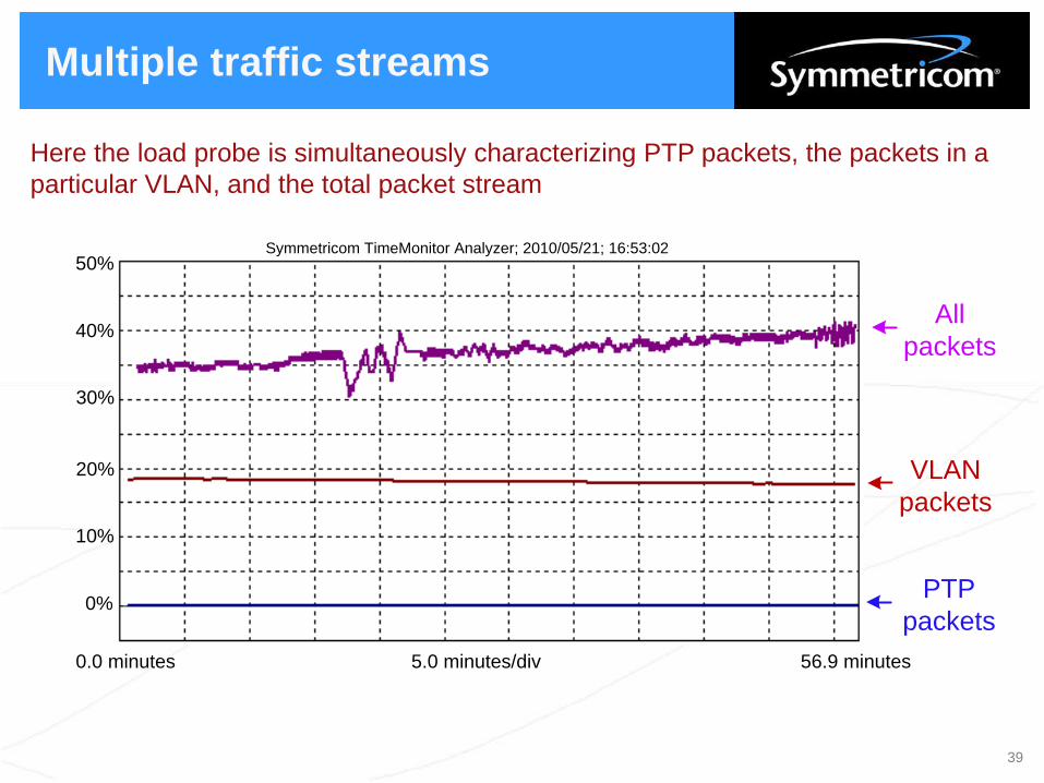
Multiple traffic streams
Here the load probe is simultaneously characterizing PTP packets, the packets in a
particular VLAN, and the total packet stream
39
5.0 minutes/div
50%
40%
0.0 minutes 56.9 minutes
30%
10%
0%
Symmetricom TimeMonitor Analyzer; 2010/05/21; 16:53:02
PTP
packets
VLAN
packets
All
packets
20%
Summary
Three types of measurements discussed1. “TIE”
2. Packet “PDV”
3. Packet “Load”
Clock and Packet Analysis TIE analysis methods inform approach to PDV analysis
Stability metrics (1) Preprocessed or (2) Integrated packet selection
Frequency transport metrics
Time transport metrics
Network Measurements Lab/production packet network measurements shown
Packet measurement analysis can be used to predict packet slave performance
Load Probe Third measurement type
Primary reference clock not required
“Load” and “PDV” are related
40

Lee Cosart
Senior Technologist
Phone : +1-408-428-6950
Symmetricom
2300 Orchard Parkway
San Jose, California, 95131
United States of America
www.symmetricom.com