Package ‘wavethresh’ - The Comprehensive R Archive … · Package ‘wavethresh’ October 20, 2016 Type Package Title Wavelets Statistics and Transforms Version 4.6.8 Date 2016-10-18

Package ‘wavethresh’October 20, 2016

Type Package

Title Wavelets Statistics and Transforms

Version 4.6.8

Date 2016-10-18

Depends R (>= 2.10), MASS

Description Performs 1, 2 and 3D real and complex-valued wavelet transforms,nondecimated transforms, wavelet packet transforms, nondecimatedwavelet packet transforms, multiple wavelet transforms,complex-valued wavelet transforms, wavelet shrinkage forvarious kinds of data, locally stationary wavelet time series,nonstationary multiscale transfer function modeling, densityestimation.

License GPL (>= 2)

NeedsCompilation yes

Author Guy Nason [aut, cre]

Maintainer Guy Nason <[email protected]>

Repository CRAN

Date/Publication 2016-10-20 15:33:30

R topics documented:wavethresh-package . . . . . . . . . . . . . . . . . . . . . . . . . . . . . . . . . . . . . 7accessC . . . . . . . . . . . . . . . . . . . . . . . . . . . . . . . . . . . . . . . . . . . 8accessc . . . . . . . . . . . . . . . . . . . . . . . . . . . . . . . . . . . . . . . . . . . 9accessC.mwd . . . . . . . . . . . . . . . . . . . . . . . . . . . . . . . . . . . . . . . . 10accessC.wd . . . . . . . . . . . . . . . . . . . . . . . . . . . . . . . . . . . . . . . . . 11accessC.wp . . . . . . . . . . . . . . . . . . . . . . . . . . . . . . . . . . . . . . . . . 13accessC.wst . . . . . . . . . . . . . . . . . . . . . . . . . . . . . . . . . . . . . . . . . 14accessD . . . . . . . . . . . . . . . . . . . . . . . . . . . . . . . . . . . . . . . . . . . 15accessD.mwd . . . . . . . . . . . . . . . . . . . . . . . . . . . . . . . . . . . . . . . . 16accessD.wd . . . . . . . . . . . . . . . . . . . . . . . . . . . . . . . . . . . . . . . . . 17accessD.wd3D . . . . . . . . . . . . . . . . . . . . . . . . . . . . . . . . . . . . . . . 19

1

2 R topics documented:

accessD.wp . . . . . . . . . . . . . . . . . . . . . . . . . . . . . . . . . . . . . . . . . 21accessD.wpst . . . . . . . . . . . . . . . . . . . . . . . . . . . . . . . . . . . . . . . . 22accessD.wst . . . . . . . . . . . . . . . . . . . . . . . . . . . . . . . . . . . . . . . . . 24addpkt . . . . . . . . . . . . . . . . . . . . . . . . . . . . . . . . . . . . . . . . . . . . 25AutoBasis . . . . . . . . . . . . . . . . . . . . . . . . . . . . . . . . . . . . . . . . . . 26av.basis . . . . . . . . . . . . . . . . . . . . . . . . . . . . . . . . . . . . . . . . . . . 26AvBasis . . . . . . . . . . . . . . . . . . . . . . . . . . . . . . . . . . . . . . . . . . . 27AvBasis.wst . . . . . . . . . . . . . . . . . . . . . . . . . . . . . . . . . . . . . . . . . 28AvBasis.wst2D . . . . . . . . . . . . . . . . . . . . . . . . . . . . . . . . . . . . . . . 30BabyECG . . . . . . . . . . . . . . . . . . . . . . . . . . . . . . . . . . . . . . . . . . 32BabySS . . . . . . . . . . . . . . . . . . . . . . . . . . . . . . . . . . . . . . . . . . . 34basisplot . . . . . . . . . . . . . . . . . . . . . . . . . . . . . . . . . . . . . . . . . . . 36basisplot.BP . . . . . . . . . . . . . . . . . . . . . . . . . . . . . . . . . . . . . . . . . 37basisplot.wp . . . . . . . . . . . . . . . . . . . . . . . . . . . . . . . . . . . . . . . . . 38BAYES.THR . . . . . . . . . . . . . . . . . . . . . . . . . . . . . . . . . . . . . . . . 39Best1DCols . . . . . . . . . . . . . . . . . . . . . . . . . . . . . . . . . . . . . . . . . 41bestm . . . . . . . . . . . . . . . . . . . . . . . . . . . . . . . . . . . . . . . . . . . . 42BMdiscr . . . . . . . . . . . . . . . . . . . . . . . . . . . . . . . . . . . . . . . . . . . 43c2to4 . . . . . . . . . . . . . . . . . . . . . . . . . . . . . . . . . . . . . . . . . . . . 44CanUseMoreThanOneColor . . . . . . . . . . . . . . . . . . . . . . . . . . . . . . . . 45checkmyews . . . . . . . . . . . . . . . . . . . . . . . . . . . . . . . . . . . . . . . . . 45Chires5 . . . . . . . . . . . . . . . . . . . . . . . . . . . . . . . . . . . . . . . . . . . 46Chires6 . . . . . . . . . . . . . . . . . . . . . . . . . . . . . . . . . . . . . . . . . . . 47cns . . . . . . . . . . . . . . . . . . . . . . . . . . . . . . . . . . . . . . . . . . . . . . 48compare.filters . . . . . . . . . . . . . . . . . . . . . . . . . . . . . . . . . . . . . . . 49compgrot . . . . . . . . . . . . . . . . . . . . . . . . . . . . . . . . . . . . . . . . . . 50compress . . . . . . . . . . . . . . . . . . . . . . . . . . . . . . . . . . . . . . . . . . 52compress.default . . . . . . . . . . . . . . . . . . . . . . . . . . . . . . . . . . . . . . 53compress.imwd . . . . . . . . . . . . . . . . . . . . . . . . . . . . . . . . . . . . . . . 54conbar . . . . . . . . . . . . . . . . . . . . . . . . . . . . . . . . . . . . . . . . . . . . 55convert . . . . . . . . . . . . . . . . . . . . . . . . . . . . . . . . . . . . . . . . . . . . 57convert.wd . . . . . . . . . . . . . . . . . . . . . . . . . . . . . . . . . . . . . . . . . . 58convert.wst . . . . . . . . . . . . . . . . . . . . . . . . . . . . . . . . . . . . . . . . . 60ConvertMessage . . . . . . . . . . . . . . . . . . . . . . . . . . . . . . . . . . . . . . . 62Crsswav . . . . . . . . . . . . . . . . . . . . . . . . . . . . . . . . . . . . . . . . . . . 63cthresh . . . . . . . . . . . . . . . . . . . . . . . . . . . . . . . . . . . . . . . . . . . . 64Cthreshold . . . . . . . . . . . . . . . . . . . . . . . . . . . . . . . . . . . . . . . . . . 66CWavDE . . . . . . . . . . . . . . . . . . . . . . . . . . . . . . . . . . . . . . . . . . 67CWCV . . . . . . . . . . . . . . . . . . . . . . . . . . . . . . . . . . . . . . . . . . . 69dclaw . . . . . . . . . . . . . . . . . . . . . . . . . . . . . . . . . . . . . . . . . . . . 71dencvwd . . . . . . . . . . . . . . . . . . . . . . . . . . . . . . . . . . . . . . . . . . . 72denplot . . . . . . . . . . . . . . . . . . . . . . . . . . . . . . . . . . . . . . . . . . . 73denproj . . . . . . . . . . . . . . . . . . . . . . . . . . . . . . . . . . . . . . . . . . . 74denwd . . . . . . . . . . . . . . . . . . . . . . . . . . . . . . . . . . . . . . . . . . . . 76denwr . . . . . . . . . . . . . . . . . . . . . . . . . . . . . . . . . . . . . . . . . . . . 77DJ.EX . . . . . . . . . . . . . . . . . . . . . . . . . . . . . . . . . . . . . . . . . . . . 78dof . . . . . . . . . . . . . . . . . . . . . . . . . . . . . . . . . . . . . . . . . . . . . . 79doppler . . . . . . . . . . . . . . . . . . . . . . . . . . . . . . . . . . . . . . . . . . . 80

R topics documented: 3

draw . . . . . . . . . . . . . . . . . . . . . . . . . . . . . . . . . . . . . . . . . . . . . 81draw.default . . . . . . . . . . . . . . . . . . . . . . . . . . . . . . . . . . . . . . . . . 82draw.imwd . . . . . . . . . . . . . . . . . . . . . . . . . . . . . . . . . . . . . . . . . . 85draw.imwdc . . . . . . . . . . . . . . . . . . . . . . . . . . . . . . . . . . . . . . . . . 86draw.mwd . . . . . . . . . . . . . . . . . . . . . . . . . . . . . . . . . . . . . . . . . . 88draw.wd . . . . . . . . . . . . . . . . . . . . . . . . . . . . . . . . . . . . . . . . . . . 89draw.wp . . . . . . . . . . . . . . . . . . . . . . . . . . . . . . . . . . . . . . . . . . . 90draw.wst . . . . . . . . . . . . . . . . . . . . . . . . . . . . . . . . . . . . . . . . . . . 92drawbox . . . . . . . . . . . . . . . . . . . . . . . . . . . . . . . . . . . . . . . . . . . 93drawwp.default . . . . . . . . . . . . . . . . . . . . . . . . . . . . . . . . . . . . . . . 94ewspec . . . . . . . . . . . . . . . . . . . . . . . . . . . . . . . . . . . . . . . . . . . . 95example.1 . . . . . . . . . . . . . . . . . . . . . . . . . . . . . . . . . . . . . . . . . . 98filter.select . . . . . . . . . . . . . . . . . . . . . . . . . . . . . . . . . . . . . . . . . . 99find.parameters . . . . . . . . . . . . . . . . . . . . . . . . . . . . . . . . . . . . . . . 102first.last . . . . . . . . . . . . . . . . . . . . . . . . . . . . . . . . . . . . . . . . . . . 103first.last.dh . . . . . . . . . . . . . . . . . . . . . . . . . . . . . . . . . . . . . . . . . . 106firstdot . . . . . . . . . . . . . . . . . . . . . . . . . . . . . . . . . . . . . . . . . . . . 107FullWaveletCV . . . . . . . . . . . . . . . . . . . . . . . . . . . . . . . . . . . . . . . 108GenW . . . . . . . . . . . . . . . . . . . . . . . . . . . . . . . . . . . . . . . . . . . . 109getarrvec . . . . . . . . . . . . . . . . . . . . . . . . . . . . . . . . . . . . . . . . . . 111getpacket . . . . . . . . . . . . . . . . . . . . . . . . . . . . . . . . . . . . . . . . . . 113getpacket.wp . . . . . . . . . . . . . . . . . . . . . . . . . . . . . . . . . . . . . . . . 114getpacket.wpst . . . . . . . . . . . . . . . . . . . . . . . . . . . . . . . . . . . . . . . 116getpacket.wst . . . . . . . . . . . . . . . . . . . . . . . . . . . . . . . . . . . . . . . . 118getpacket.wst2D . . . . . . . . . . . . . . . . . . . . . . . . . . . . . . . . . . . . . . . 120GetRSSWST . . . . . . . . . . . . . . . . . . . . . . . . . . . . . . . . . . . . . . . . 123griddata objects . . . . . . . . . . . . . . . . . . . . . . . . . . . . . . . . . . . . . . . 124guyrot . . . . . . . . . . . . . . . . . . . . . . . . . . . . . . . . . . . . . . . . . . . . 126HaarConcat . . . . . . . . . . . . . . . . . . . . . . . . . . . . . . . . . . . . . . . . . 127HaarMA . . . . . . . . . . . . . . . . . . . . . . . . . . . . . . . . . . . . . . . . . . . 128image.wd . . . . . . . . . . . . . . . . . . . . . . . . . . . . . . . . . . . . . . . . . . 130image.wst . . . . . . . . . . . . . . . . . . . . . . . . . . . . . . . . . . . . . . . . . . 131imwd . . . . . . . . . . . . . . . . . . . . . . . . . . . . . . . . . . . . . . . . . . . . 132imwd.object . . . . . . . . . . . . . . . . . . . . . . . . . . . . . . . . . . . . . . . . . 134imwdc.object . . . . . . . . . . . . . . . . . . . . . . . . . . . . . . . . . . . . . . . . 135imwr . . . . . . . . . . . . . . . . . . . . . . . . . . . . . . . . . . . . . . . . . . . . . 138imwr.imwd . . . . . . . . . . . . . . . . . . . . . . . . . . . . . . . . . . . . . . . . . 139imwr.imwdc . . . . . . . . . . . . . . . . . . . . . . . . . . . . . . . . . . . . . . . . . 140InvBasis . . . . . . . . . . . . . . . . . . . . . . . . . . . . . . . . . . . . . . . . . . . 142InvBasis.wp . . . . . . . . . . . . . . . . . . . . . . . . . . . . . . . . . . . . . . . . . 143InvBasis.wst . . . . . . . . . . . . . . . . . . . . . . . . . . . . . . . . . . . . . . . . . 144ipd . . . . . . . . . . . . . . . . . . . . . . . . . . . . . . . . . . . . . . . . . . . . . . 145ipndacw . . . . . . . . . . . . . . . . . . . . . . . . . . . . . . . . . . . . . . . . . . . 146irregwd . . . . . . . . . . . . . . . . . . . . . . . . . . . . . . . . . . . . . . . . . . . 149irregwd.objects . . . . . . . . . . . . . . . . . . . . . . . . . . . . . . . . . . . . . . . 151IsEarly . . . . . . . . . . . . . . . . . . . . . . . . . . . . . . . . . . . . . . . . . . . . 152IsEarly.default . . . . . . . . . . . . . . . . . . . . . . . . . . . . . . . . . . . . . . . . 153IsEarly.wd . . . . . . . . . . . . . . . . . . . . . . . . . . . . . . . . . . . . . . . . . . 153


IsPowerOfTwo . . . . . . . . . . . . . . . . . . . . . . . . . . . . . . . . . . . . . . . 154l2norm . . . . . . . . . . . . . . . . . . . . . . . . . . . . . . . . . . . . . . . . . . . . 155lennon . . . . . . . . . . . . . . . . . . . . . . . . . . . . . . . . . . . . . . . . . . . . 156levarr . . . . . . . . . . . . . . . . . . . . . . . . . . . . . . . . . . . . . . . . . . . . 157linfnorm . . . . . . . . . . . . . . . . . . . . . . . . . . . . . . . . . . . . . . . . . . . 158LocalSpec . . . . . . . . . . . . . . . . . . . . . . . . . . . . . . . . . . . . . . . . . . 159LocalSpec.wd . . . . . . . . . . . . . . . . . . . . . . . . . . . . . . . . . . . . . . . . 160LocalSpec.wst . . . . . . . . . . . . . . . . . . . . . . . . . . . . . . . . . . . . . . . . 163logabs . . . . . . . . . . . . . . . . . . . . . . . . . . . . . . . . . . . . . . . . . . . . 164LSWsim . . . . . . . . . . . . . . . . . . . . . . . . . . . . . . . . . . . . . . . . . . . 165lt.to.name . . . . . . . . . . . . . . . . . . . . . . . . . . . . . . . . . . . . . . . . . . 168madmad . . . . . . . . . . . . . . . . . . . . . . . . . . . . . . . . . . . . . . . . . . . 169make.dwwt . . . . . . . . . . . . . . . . . . . . . . . . . . . . . . . . . . . . . . . . . 171makegrid . . . . . . . . . . . . . . . . . . . . . . . . . . . . . . . . . . . . . . . . . . 172makewpstDO . . . . . . . . . . . . . . . . . . . . . . . . . . . . . . . . . . . . . . . . 174makewpstRO . . . . . . . . . . . . . . . . . . . . . . . . . . . . . . . . . . . . . . . . 177MaNoVe . . . . . . . . . . . . . . . . . . . . . . . . . . . . . . . . . . . . . . . . . . . 182MaNoVe.wp . . . . . . . . . . . . . . . . . . . . . . . . . . . . . . . . . . . . . . . . . 183MaNoVe.wst . . . . . . . . . . . . . . . . . . . . . . . . . . . . . . . . . . . . . . . . 184mfilter.select . . . . . . . . . . . . . . . . . . . . . . . . . . . . . . . . . . . . . . . . . 187mfirst.last . . . . . . . . . . . . . . . . . . . . . . . . . . . . . . . . . . . . . . . . . . 189modernise . . . . . . . . . . . . . . . . . . . . . . . . . . . . . . . . . . . . . . . . . . 191modernise.wd . . . . . . . . . . . . . . . . . . . . . . . . . . . . . . . . . . . . . . . . 192mpostfilter . . . . . . . . . . . . . . . . . . . . . . . . . . . . . . . . . . . . . . . . . . 192mprefilter . . . . . . . . . . . . . . . . . . . . . . . . . . . . . . . . . . . . . . . . . . 193mwd . . . . . . . . . . . . . . . . . . . . . . . . . . . . . . . . . . . . . . . . . . . . . 194mwd.object . . . . . . . . . . . . . . . . . . . . . . . . . . . . . . . . . . . . . . . . . 196mwr . . . . . . . . . . . . . . . . . . . . . . . . . . . . . . . . . . . . . . . . . . . . . 198newsure . . . . . . . . . . . . . . . . . . . . . . . . . . . . . . . . . . . . . . . . . . . 199nlevelsWT . . . . . . . . . . . . . . . . . . . . . . . . . . . . . . . . . . . . . . . . . . 200nlevelsWT.default . . . . . . . . . . . . . . . . . . . . . . . . . . . . . . . . . . . . . . 201nullevels . . . . . . . . . . . . . . . . . . . . . . . . . . . . . . . . . . . . . . . . . . . 202nullevels.imwd . . . . . . . . . . . . . . . . . . . . . . . . . . . . . . . . . . . . . . . 203nullevels.wd . . . . . . . . . . . . . . . . . . . . . . . . . . . . . . . . . . . . . . . . . 204nullevels.wst . . . . . . . . . . . . . . . . . . . . . . . . . . . . . . . . . . . . . . . . 206numtonv . . . . . . . . . . . . . . . . . . . . . . . . . . . . . . . . . . . . . . . . . . . 207nv.object . . . . . . . . . . . . . . . . . . . . . . . . . . . . . . . . . . . . . . . . . . . 209plot.imwd . . . . . . . . . . . . . . . . . . . . . . . . . . . . . . . . . . . . . . . . . . 210plot.irregwd . . . . . . . . . . . . . . . . . . . . . . . . . . . . . . . . . . . . . . . . . 211plot.mwd . . . . . . . . . . . . . . . . . . . . . . . . . . . . . . . . . . . . . . . . . . 213plot.nvwp . . . . . . . . . . . . . . . . . . . . . . . . . . . . . . . . . . . . . . . . . . 215plot.wd . . . . . . . . . . . . . . . . . . . . . . . . . . . . . . . . . . . . . . . . . . . 216plot.wp . . . . . . . . . . . . . . . . . . . . . . . . . . . . . . . . . . . . . . . . . . . 219plot.wst . . . . . . . . . . . . . . . . . . . . . . . . . . . . . . . . . . . . . . . . . . . 222plot.wst2D . . . . . . . . . . . . . . . . . . . . . . . . . . . . . . . . . . . . . . . . . . 224plotdenwd . . . . . . . . . . . . . . . . . . . . . . . . . . . . . . . . . . . . . . . . . . 225plotpkt . . . . . . . . . . . . . . . . . . . . . . . . . . . . . . . . . . . . . . . . . . . . 227print.BP . . . . . . . . . . . . . . . . . . . . . . . . . . . . . . . . . . . . . . . . . . . 228

R topics documented: 5

print.imwd . . . . . . . . . . . . . . . . . . . . . . . . . . . . . . . . . . . . . . . . . . 228print.imwdc . . . . . . . . . . . . . . . . . . . . . . . . . . . . . . . . . . . . . . . . . 230print.mwd . . . . . . . . . . . . . . . . . . . . . . . . . . . . . . . . . . . . . . . . . . 231print.nv . . . . . . . . . . . . . . . . . . . . . . . . . . . . . . . . . . . . . . . . . . . 233print.nvwp . . . . . . . . . . . . . . . . . . . . . . . . . . . . . . . . . . . . . . . . . . 234print.w2d . . . . . . . . . . . . . . . . . . . . . . . . . . . . . . . . . . . . . . . . . . 236print.w2m . . . . . . . . . . . . . . . . . . . . . . . . . . . . . . . . . . . . . . . . . . 237print.wd . . . . . . . . . . . . . . . . . . . . . . . . . . . . . . . . . . . . . . . . . . . 238print.wd3D . . . . . . . . . . . . . . . . . . . . . . . . . . . . . . . . . . . . . . . . . 239print.wp . . . . . . . . . . . . . . . . . . . . . . . . . . . . . . . . . . . . . . . . . . . 240print.wpst . . . . . . . . . . . . . . . . . . . . . . . . . . . . . . . . . . . . . . . . . . 242print.wpstCL . . . . . . . . . . . . . . . . . . . . . . . . . . . . . . . . . . . . . . . . 243print.wpstDO . . . . . . . . . . . . . . . . . . . . . . . . . . . . . . . . . . . . . . . . 244print.wpstRO . . . . . . . . . . . . . . . . . . . . . . . . . . . . . . . . . . . . . . . . 246print.wst . . . . . . . . . . . . . . . . . . . . . . . . . . . . . . . . . . . . . . . . . . . 247print.wst2D . . . . . . . . . . . . . . . . . . . . . . . . . . . . . . . . . . . . . . . . . 248PsiJ . . . . . . . . . . . . . . . . . . . . . . . . . . . . . . . . . . . . . . . . . . . . . 249PsiJmat . . . . . . . . . . . . . . . . . . . . . . . . . . . . . . . . . . . . . . . . . . . 252Psiname . . . . . . . . . . . . . . . . . . . . . . . . . . . . . . . . . . . . . . . . . . . 255putC . . . . . . . . . . . . . . . . . . . . . . . . . . . . . . . . . . . . . . . . . . . . . 256putC.mwd . . . . . . . . . . . . . . . . . . . . . . . . . . . . . . . . . . . . . . . . . . 257putC.wd . . . . . . . . . . . . . . . . . . . . . . . . . . . . . . . . . . . . . . . . . . . 259putC.wp . . . . . . . . . . . . . . . . . . . . . . . . . . . . . . . . . . . . . . . . . . . 261putC.wst . . . . . . . . . . . . . . . . . . . . . . . . . . . . . . . . . . . . . . . . . . . 262putD . . . . . . . . . . . . . . . . . . . . . . . . . . . . . . . . . . . . . . . . . . . . . 264putD.mwd . . . . . . . . . . . . . . . . . . . . . . . . . . . . . . . . . . . . . . . . . . 265putD.wd . . . . . . . . . . . . . . . . . . . . . . . . . . . . . . . . . . . . . . . . . . . 267putD.wd3D . . . . . . . . . . . . . . . . . . . . . . . . . . . . . . . . . . . . . . . . . 269putD.wp . . . . . . . . . . . . . . . . . . . . . . . . . . . . . . . . . . . . . . . . . . . 270putD.wst . . . . . . . . . . . . . . . . . . . . . . . . . . . . . . . . . . . . . . . . . . . 272putDwd3Dcheck . . . . . . . . . . . . . . . . . . . . . . . . . . . . . . . . . . . . . . 273putpacket . . . . . . . . . . . . . . . . . . . . . . . . . . . . . . . . . . . . . . . . . . 274putpacket.wp . . . . . . . . . . . . . . . . . . . . . . . . . . . . . . . . . . . . . . . . 275putpacket.wst . . . . . . . . . . . . . . . . . . . . . . . . . . . . . . . . . . . . . . . . 277putpacket.wst2D . . . . . . . . . . . . . . . . . . . . . . . . . . . . . . . . . . . . . . 279rcov . . . . . . . . . . . . . . . . . . . . . . . . . . . . . . . . . . . . . . . . . . . . . 281rfft . . . . . . . . . . . . . . . . . . . . . . . . . . . . . . . . . . . . . . . . . . . . . . 282rfftinv . . . . . . . . . . . . . . . . . . . . . . . . . . . . . . . . . . . . . . . . . . . . 283rfftwt . . . . . . . . . . . . . . . . . . . . . . . . . . . . . . . . . . . . . . . . . . . . 284rm.det . . . . . . . . . . . . . . . . . . . . . . . . . . . . . . . . . . . . . . . . . . . . 284rmget . . . . . . . . . . . . . . . . . . . . . . . . . . . . . . . . . . . . . . . . . . . . 285rmname . . . . . . . . . . . . . . . . . . . . . . . . . . . . . . . . . . . . . . . . . . . 287rotateback . . . . . . . . . . . . . . . . . . . . . . . . . . . . . . . . . . . . . . . . . . 288rsswav . . . . . . . . . . . . . . . . . . . . . . . . . . . . . . . . . . . . . . . . . . . . 289ScalingFunction . . . . . . . . . . . . . . . . . . . . . . . . . . . . . . . . . . . . . . . 291Shannon.entropy . . . . . . . . . . . . . . . . . . . . . . . . . . . . . . . . . . . . . . 292simchirp . . . . . . . . . . . . . . . . . . . . . . . . . . . . . . . . . . . . . . . . . . . 293ssq . . . . . . . . . . . . . . . . . . . . . . . . . . . . . . . . . . . . . . . . . . . . . . 294


summary.imwd . . . . . . . . . . . . . . . . . . . . . . . . . . . . . . . . . . . . . . . 295summary.imwdc . . . . . . . . . . . . . . . . . . . . . . . . . . . . . . . . . . . . . . . 296summary.mwd . . . . . . . . . . . . . . . . . . . . . . . . . . . . . . . . . . . . . . . . 297summary.wd . . . . . . . . . . . . . . . . . . . . . . . . . . . . . . . . . . . . . . . . . 298summary.wd3D . . . . . . . . . . . . . . . . . . . . . . . . . . . . . . . . . . . . . . . 299summary.wp . . . . . . . . . . . . . . . . . . . . . . . . . . . . . . . . . . . . . . . . . 300summary.wpst . . . . . . . . . . . . . . . . . . . . . . . . . . . . . . . . . . . . . . . . 301summary.wst . . . . . . . . . . . . . . . . . . . . . . . . . . . . . . . . . . . . . . . . 302summary.wst2D . . . . . . . . . . . . . . . . . . . . . . . . . . . . . . . . . . . . . . . 303support . . . . . . . . . . . . . . . . . . . . . . . . . . . . . . . . . . . . . . . . . . . 304sure . . . . . . . . . . . . . . . . . . . . . . . . . . . . . . . . . . . . . . . . . . . . . 305teddy . . . . . . . . . . . . . . . . . . . . . . . . . . . . . . . . . . . . . . . . . . . . 306test.dataCT . . . . . . . . . . . . . . . . . . . . . . . . . . . . . . . . . . . . . . . . . 307threshold . . . . . . . . . . . . . . . . . . . . . . . . . . . . . . . . . . . . . . . . . . 308threshold.imwd . . . . . . . . . . . . . . . . . . . . . . . . . . . . . . . . . . . . . . . 309threshold.imwdc . . . . . . . . . . . . . . . . . . . . . . . . . . . . . . . . . . . . . . . 313threshold.irregwd . . . . . . . . . . . . . . . . . . . . . . . . . . . . . . . . . . . . . . 314threshold.mwd . . . . . . . . . . . . . . . . . . . . . . . . . . . . . . . . . . . . . . . 316threshold.wd . . . . . . . . . . . . . . . . . . . . . . . . . . . . . . . . . . . . . . . . . 319threshold.wd3D . . . . . . . . . . . . . . . . . . . . . . . . . . . . . . . . . . . . . . . 324threshold.wp . . . . . . . . . . . . . . . . . . . . . . . . . . . . . . . . . . . . . . . . . 327threshold.wst . . . . . . . . . . . . . . . . . . . . . . . . . . . . . . . . . . . . . . . . 330TOgetthrda1 . . . . . . . . . . . . . . . . . . . . . . . . . . . . . . . . . . . . . . . . . 334TOthreshda1 . . . . . . . . . . . . . . . . . . . . . . . . . . . . . . . . . . . . . . . . 335TOthreshda2 . . . . . . . . . . . . . . . . . . . . . . . . . . . . . . . . . . . . . . . . 336tpwd . . . . . . . . . . . . . . . . . . . . . . . . . . . . . . . . . . . . . . . . . . . . . 337tpwr . . . . . . . . . . . . . . . . . . . . . . . . . . . . . . . . . . . . . . . . . . . . . 338uncompress . . . . . . . . . . . . . . . . . . . . . . . . . . . . . . . . . . . . . . . . . 339uncompress.default . . . . . . . . . . . . . . . . . . . . . . . . . . . . . . . . . . . . . 340uncompress.imwdc . . . . . . . . . . . . . . . . . . . . . . . . . . . . . . . . . . . . . 341wavegrow . . . . . . . . . . . . . . . . . . . . . . . . . . . . . . . . . . . . . . . . . . 342WaveletCV . . . . . . . . . . . . . . . . . . . . . . . . . . . . . . . . . . . . . . . . . 344wd . . . . . . . . . . . . . . . . . . . . . . . . . . . . . . . . . . . . . . . . . . . . . . 345wd.dh . . . . . . . . . . . . . . . . . . . . . . . . . . . . . . . . . . . . . . . . . . . . 350wd.int . . . . . . . . . . . . . . . . . . . . . . . . . . . . . . . . . . . . . . . . . . . . 351wd.object . . . . . . . . . . . . . . . . . . . . . . . . . . . . . . . . . . . . . . . . . . 352wd3D . . . . . . . . . . . . . . . . . . . . . . . . . . . . . . . . . . . . . . . . . . . . 354wd3D.object . . . . . . . . . . . . . . . . . . . . . . . . . . . . . . . . . . . . . . . . . 355Whistory . . . . . . . . . . . . . . . . . . . . . . . . . . . . . . . . . . . . . . . . . . 356Whistory.wst . . . . . . . . . . . . . . . . . . . . . . . . . . . . . . . . . . . . . . . . 357wp . . . . . . . . . . . . . . . . . . . . . . . . . . . . . . . . . . . . . . . . . . . . . . 358wp.object . . . . . . . . . . . . . . . . . . . . . . . . . . . . . . . . . . . . . . . . . . 359wpst . . . . . . . . . . . . . . . . . . . . . . . . . . . . . . . . . . . . . . . . . . . . . 360wpst2discr . . . . . . . . . . . . . . . . . . . . . . . . . . . . . . . . . . . . . . . . . . 362wpst2m . . . . . . . . . . . . . . . . . . . . . . . . . . . . . . . . . . . . . . . . . . . 363wpstCLASS . . . . . . . . . . . . . . . . . . . . . . . . . . . . . . . . . . . . . . . . . 364wpstREGR . . . . . . . . . . . . . . . . . . . . . . . . . . . . . . . . . . . . . . . . . 365wr . . . . . . . . . . . . . . . . . . . . . . . . . . . . . . . . . . . . . . . . . . . . . . 366

wavethresh-package 7

wr.int . . . . . . . . . . . . . . . . . . . . . . . . . . . . . . . . . . . . . . . . . . . . 367wr.mwd . . . . . . . . . . . . . . . . . . . . . . . . . . . . . . . . . . . . . . . . . . . 368wr.wd . . . . . . . . . . . . . . . . . . . . . . . . . . . . . . . . . . . . . . . . . . . . 369wr3D . . . . . . . . . . . . . . . . . . . . . . . . . . . . . . . . . . . . . . . . . . . . 371wst . . . . . . . . . . . . . . . . . . . . . . . . . . . . . . . . . . . . . . . . . . . . . . 372wst.object . . . . . . . . . . . . . . . . . . . . . . . . . . . . . . . . . . . . . . . . . . 374wst2D . . . . . . . . . . . . . . . . . . . . . . . . . . . . . . . . . . . . . . . . . . . . 375wst2D.object . . . . . . . . . . . . . . . . . . . . . . . . . . . . . . . . . . . . . . . . 377wstCV . . . . . . . . . . . . . . . . . . . . . . . . . . . . . . . . . . . . . . . . . . . . 379wstCVl . . . . . . . . . . . . . . . . . . . . . . . . . . . . . . . . . . . . . . . . . . . 381WTEnv . . . . . . . . . . . . . . . . . . . . . . . . . . . . . . . . . . . . . . . . . . . 384wvcvlrss . . . . . . . . . . . . . . . . . . . . . . . . . . . . . . . . . . . . . . . . . . . 385wvmoments . . . . . . . . . . . . . . . . . . . . . . . . . . . . . . . . . . . . . . . . . 386wvrelease . . . . . . . . . . . . . . . . . . . . . . . . . . . . . . . . . . . . . . . . . . 387

Index 389

wavethresh-package Wavelet transforms and associated statistical methodology.

Description

Performs one-, two- and three-dimensional wavelet transforms, nondecimated transforms, waveletpacket transforms, nondecimated wavelet packet transforms, complex-valued wavelet transforms,wavelet shrinkage for various kinds of data, locally stationary wavelet time series, nonstationarymultiscale transfer function modeling, density estimation.

Details

Package: wavethreshType: PackageVersion: 4.6.6Date: 2013-10-21License: GPL (>=2)

Author(s)

Guy Nason, <[email protected]>

References

Nason, G.P. (2008) Wavelet methods in Statistics with R. Springer, New York. Book URL.

Errata and fast-breaking news: http://www.stats.bris.ac.uk/~wavethresh

http://www.springer.com/statistics/statistical+theory+and+methods/book/978-0-387-75960-9

http://www.stats.bris.ac.uk/~wavethresh

8 accessC

See Also

ewspec, imwd, threshold, wd, wst

Examples

## See examples in individual help pages#

accessC Get "detail" (mother wavelet) coefficients data from wavelet object

Description

This generic function extracts detail from various types of wavelet objects. It extracts and returnsa whole resolution level of coefficients. To obtain individual packets from relevant transforms usethe getpacket() series of functions. This function is generic.

Particular methods exist. For objects of class:

wd use the accessC.wd method

wp use the accessC.wp method

wst use the accessC.wst method

See individual method help pages for operation and examples.

Usage

accessC(...)

Arguments

... See individual help for details.

Value

A vector coefficients representing the detail coefficients for the requested resolution level.

RELEASE

Version 3.5.3 Copyright Guy Nason 1994

Author(s)

G P Nason

See Also

accessC.wd, accessC.wp,accessC.wst,accessD

accessc 9

accessc Get variance information from irregularly spaced wavelet decomposi-tion object.

Description

This function gets information from the c component of an irregwd.objects an irregularly spacedwavelet decomposition object.

Note that this function is not the same as accessC which obtains father wavelet coefficients froman wd class object.

Usage

accessc(irregwd.structure, level, boundary=FALSE)

Arguments

irregwd.structure

Irregular wavelet decomposition object from which you wish to extract parts ofthe c component from.

level The level that you wish to extract. This value ranges from 0 to the nlevelsWT(irregwd.structure)-1.

boundary If this argument is T then all of the boundary correction values will be returnedas well (note: the length of the returned vector may not be a power of 2). Ifboundary is false, then just the coefficients will be returned. If the decompo-sition (or reconstruction) was done with periodic boundary conditions then thisoption has no effect.

Details

The irregwd function produces a irregular wavelet decomposition (reconstruction) structure.

The c component is stored in a similar way to the C and D vectors which store the father andmother wavelet coefficients respectively. Hence to access the information the accessc functionplays a similar role to accessC and accessD functions.

Value

A vector of the extracted data.

RELEASE

Version 3.9.4 Code Copyright Arne Kovac 1997. Help Copyright Guy Nason 2004.

Author(s)

G P Nason

10 accessC.mwd

See Also

irregwd, irregwd.objects, threshold.irregwd,makegrid, plot.irregwd

Examples

## Most users will not need to use this function. However, see the main# examples for the irregular wavelet denoising in the examples for# makegrid.#

accessC.mwd Get Smoothed Data from Wavelet Structure

Description

The smoothed and original data from a multiple wavelet decomposition structure, mwd.object ect(e.g. returned from mwd) are packed into a single matrix in that structure. TRUE his function extractsthe data corresponding to a particular resolution level.

Usage

## S3 method for class 'mwd'accessC(mwd, level = nlevelsWT(mwd), ...)

Arguments

mwd Multiple wavelet decomposition structure from which you wish to extract thesmoothed or original data if the structure is from a wavelet decomposition, orthe reconstructed data if the structure is from a wavelet reconstruction.

level The level that you wish to extract. By default, this is the level with most detail(in the case of structures from a decomposition this is the original data, in thecase of structures from a reconstruction this is the top-level reconstruction).

... any other arguments

Details

The mwd function produces a wavelet decomposition structure.

For decomposition, the top level contains the original data, and subsequent lower levels contain thesuccessively smoothed data. So if there are mwd$filter$npsi*2^m original data points (mwd$filter$npsiis the multiplicity of wavelets), there will be m+1 levels indexed 0,1,...,m. So

accessC.mwd(Mwd, level=m)

pulls out the original data, as does

accessC.mwd(mwd)

To get hold of lower levels just specify the level that you’re interested in, e.g.

accessC.wd 11

accessC.mwd(mwd, level=2)

Gets hold of the second level.

The need for this function is a consequence of the pyramidal structure of Mallat’s algorithm andthe memory efficiency gain achieved by storing the pyramid as a linear matrix of coefficients. Ac-cessC obtains information about where the smoothed data appears from the fl.dbase componentof mwd, in particular the array fl.dbase$first.last.c which gives a complete specification ofindex numbers and offsets for mwd$C.

Note also that this function only gets information from mwd class objects. To put coefficients intomwd structures you have to use the putC.mwd function.

See Downie and Silverman, 1998.

Value

A matrix with mwd$filter$npsi rows containing the extracted data of all the coefficients at thatlevel.

RELEASE

Version 3.9.6 (Although Copyright Tim Downie 1995-6.)

Author(s)

G P Nason

See Also

accessD.mwd, draw.mwd, mfirst.last, mfilter.select, mwd, mwd.object, mwr, plot.mwd, print.mwd,putC.mwd, putD.mwd, summary.mwd, threshold.mwd, wd

Examples

## Get the 3rd level of smoothed data from a decomposition#dat <- rnorm(32)accessC.mwd(mwd(dat), level=3)

accessC.wd Get smoothed data from wavelet object (wd)

Description

The smoothed and original data from a wavelet decomposition structure (returned from wd) arepacked into a single vector in that structure. This function extracts the data corresponding to aparticular resolution level.

12 accessC.wd

Usage

## S3 method for class 'wd'accessC(wd, level = nlevelsWT(wd), boundary=FALSE, aspect, ...)

Arguments

wd wavelet decomposition structure from which you wish to extract the smoothedor original data if the structure is from a wavelet decomposition, or the recon-structed data if the structure is from a wavelet reconstruction.

level the level that you wish to extract. By default, this is the level with most detail(in the case of structures from a decomposition this is the original data, in thecase of structures from a reconstruction this is the top-level reconstruction).

boundary logical; if TRUE then all of the boundary correction values will be returned aswell (note: the length of the returned vector may not be a power of 2).If boundary is false, then just the coefficients will be returned.If the decomposition (or reconstruction) was done with periodic boundary con-ditions, this option has no effect.

aspect Applies a function to the coefficients before return. Supplied as a text stringwhich gets converted to a function. For example, "Mod" for complex-valuedarguments


Details

The wd (wr.wd) function produces a wavelet decomposition (reconstruction) structure.

For decomposition, the top level contains the original data, and subsequent lower levels containthe successively smoothed data. So if there are 2m original data points, there will be m+1 levelsindexed 0,1,. . . ,m. So

accessC.wd(wdobj, level=m)

pulls out the original data, as does

accessC.wd(wdobj)

To get hold of lower levels just specify the level that you’re interested in, e.g.

accessC.wd(wdobj, level=2)

gets hold of the second level.

For reconstruction, the top level contains the ultimate step in the Mallat pyramid reconstructionalgorithm, lower levels are intermediate steps.

The need for this function is a consequence of the pyramidal structure of Mallat’s algorithm andthe memory efficiency gain achieved by storing the pyramid as a linear vector. AccessC obtains in-formation about where the smoothed data appears from the fl.dbase component of an wd.object, inparticular the array fl.dbase$first.last.c which gives a complete specification of index num-bers and offsets for wd.object$C.

Note that this function is method for the generic function accessC. When the wd.object is defi-nitely a wd class object then you only need use the generic version of this function.

accessC.wp 13

Note that this function only gets information from wd class objects. To insert coefficients etc. intowd structures you have to use the putC function (or more precisely, the putC.wd method).

Value


RELEASE


Author(s)

G P Nason

References

Mallat, S. G. (1989) A theory for multiresolution signal decomposition: the wavelet representation.IEEE Transactions on Pattern Analysis and Machine Intelligence 11, 674–693.

Nason, G. P. and Silverman, B. W. (1994). The discrete wavelet transform in S. Journal of Compu-tational and Graphical Statistics, 3, 163–191.

See Also

wr, wd, accessD, accessD.wd, filter.select, threshold, putC.wd, putD.wd.

Examples

## Get the 3rd level of smoothed data from a decompositiondat <- rnorm(64)accessC(wd(dat), level=3)

accessC.wp Warning function when trying to access smooths from wavelet packetobject (wp).

Description

There are no real smooths to access in a wp wavelet packet object. This function returns an er-ror message. To obtain coefficients from a wavelet packet object you should use the getpacketcollection of functions.

Usage

## S3 method for class 'wp'accessC(wp, ...)

14 accessC.wst

Arguments

wp Wavelet packet object.


Value

An error message!

RELEASE


Author(s)

G P Nason

See Also

getpacket

accessC.wst Get smoothed data from packet ordered non-decimated wavelet object(wst)

Description

The smoothed data from a packet ordered non-decimated wavelet object (returned from wst) arestored in a matrix. This function extracts all the coefficients corresponding to a particular resolutionlevel.

Usage

## S3 method for class 'wst'accessC(wst, level, aspect, ...)

Arguments

wst Packet ordered non-decimated wavelet object from which you wish to extractthe smoothed or original data (if the object is directly from a packet orderednon-decimated wavelet transform of some data).

level The level that you wish to extract. This can range from zero (the coarsest coef-ficients) to nlevelsWT(wstobj) which returns the original data.

aspect Applies function to coefficients before return. Supplied as a character stringwhich gets converted to a function. For example "Mod" which returns the abso-lute values of the coefficients

... Other arguments

accessD 15

Details

The wst function performs a packet-ordered non-decimated wavelet transform. This function ex-tracts all the father wavelet coefficients at a particular resolution level specified by level.Note that coefficients returned by this function are in emphpacket order. They can be used as isbut for many applications it might be more useful to deal with the coefficients in packets: see thefunction getpacket.wst for further details.

Value


Author(s)

G P Nason

References

Nason, G. P. and Silverman, B. W. (1994). The discrete wavelet transform in S. Journal of Compu-tational and Graphical Statistics, 3, 163–191.

See Also

wst, wst.object, accessC, getpacket.wst

Examples

## Get the 3rd level of smoothed data from a decomposition#dat <- rnorm(64)accessC(wst(dat), level=3)

accessD Get "detail" (mother wavelet) coefficients data from wavelet object

Description

This generic function extracts detail from various types of wavelet objects. It extracts and returnsa whole resolution level of coefficients. To obtain individual packets from relevant transforms usethe getpacket() series of functions. This function is generic.Particular methods exist. For objects of class:

wd use the accessD.wd methodwd3D use the accessD.wd3D methodwp use the accessD.wp methodwpst use the accessD.wpst methodwst use the accessD.wst method


16 accessD.mwd

Usage

accessD(...)

Arguments

... See individual help for details.

Value

A vector coefficients representing the detail coefficients for the requested resolution level.

RELEASE


Author(s)

G P Nason

See Also

accessD.wd, accessD.wp,accessD.wst,accessC

accessD.mwd Get wavelet coefficients from multiple wavelet structure (mwd).

Description

The wavelet coefficients from a multiple wavelet decomposition structure, mwd.object, (e.g. re-turned from mwd) are packed into a single matrix in that structure. This function extracts the coeffi-cients corresponding to a particular resolution level.

Usage

## S3 method for class 'mwd'accessD(mwd, level, ...)

Arguments

mwd Multiple wavelet decomposition structure from which you wish to extract theexpansion coefficients.

level The level that you wish to extract. If the "original" data has mwd$filter$npsi*2^mdata points (mwd$filter$npsi being the multiplicity of the multiple wavelets)then there are m possible levels that you could want to access, indexed by0,1,...,(m-1)


accessD.wd 17

Details

The mwd function produces a multiple wavelet decomposition object .

The need for this function is a consequence of the pyramidal structure of Mallats algorithm andthe memory efficiency gain achieved by storing the pyramid as a linear matrix. AccessD obtainsinformation about where the coefficients appear from the fl.dbase component of mwd, in particularthe array fl.dbase$first.last.d which gives a complete specification of index numbers andoffsets for mwd$D.

Note that this function and accessC only work on objects of class mwd to extract coefficients. Youhave to use putD.mwd to insert wavelet coefficients into a mwd object.


Value

A matrix with mwd$filter$npsi rows containing the extracted coefficients.

RELEASE

Tim Downie 1995-6

Author(s)

G P Nason

See Also

accessD.mwd, draw.mwd, mfirst.last, mfilter.select, mwd, mwd.object, plot.mwd, print.mwd,putC.mwd, putD.mwd, summary.mwd, threshold.mwd, wd, wr.mwd

Examples

## Get the 3rd level of smoothed data from a decomposition#data(ipd)accessD.mwd(mwd(ipd), level=3)

accessD.wd Get detail (mother wavelet) coefficients from wavelet object (wd).

Description

This function extracts and returns a vector of mother wavelet coefficients, corresponding to a par-ticular resolution level, from a wd wavelet decomposition object.

The pyramid of coefficients in a wavelet decomposition (returned from the wd function, say) arepacked into a single vector in WaveThresh.

18 accessD.wd

Usage

## S3 method for class 'wd'accessD(wd, level, boundary=FALSE, aspect="Identity", ...)

Arguments

wd Wavelet decomposition object from which you wish to extract the mother waveletcoefficients.

level The resolution level at which you wish to extract coefficients.

boundary some methods of wavelet transform computation handle the boundaries by keep-ing some extra bookkeeping coefficients at either end of a resolution level. Ifthis argument is TRUE then these bookkeeping coefficients are returned whenthe mother wavelets are returned. Otherwise, if FALSE, these coefficients arenot returned.

aspect The aspect argument permits the user to supply a function to modify the returnedcoefficients. The function is applied to the vector of coefficients before it isreturned. This can be useful, say, with the complex DWT where you couldsupply aspect="Mod" if you wanted to return the modulus of the coefficientsat a given resolution level. The default argument, "Identity", ensures that thecoefficients are not modified before returning.


Details

The need for this function is a consequence of the pyramidal structure of Mallat’s algorithm andthe memory efficiency gain achieved by storing the pyramid as a linear vector. AccessD obtainsinformation about where the smoothed data appears from the fl.dbase component of an wd object,in particular the array

fl.dbase$first.last.d

which gives a complete specification of index numbers and offsets for

wd.object$D.

Note that this function is a method for the generic function accessD.

Note also that this function only retrieves information from wd class objects. To insert coefficientsinto wd objects you have to use the putD function (or more precisely, the putD.wd method).

Value

A vector containing the mother wavelet coefficients at the required resolution level (the coefficientsmight have been modified depending on the value of the aspect argument).

RELEASE


Author(s)

G P Nason

accessD.wd3D 19

References

Mallat, S. G. (1989) A theory for multiresolution signal decomposition: the wavelet representation.IEEE Transactions on Pattern Analysis and Machine Intelligence. 11, 674–693.

Nason, G. P. and Silverman, B. W. (1994). The discrete wavelet transform in S. Journal of Compu-tational and Graphical Statistics, 3, 163–191

See Also

wr, wd, accessD, filter.select, threshold

Examples

## Get the 4th resolution level of wavelet coefficients.#dat <- rnorm(128)accessD(wd(dat), level=4)

accessD.wd3D Get wavelet coefficients from 3D wavelet object

Description

This function extracts and returns arrays of wavelet coefficients, corresponding to a particular reso-lution level, from a wd wavelet decomposition object.

The pyramid of coefficients in a wavelet decomposition (returned from the wd3D function, say) arepacked into a single array in WaveThresh3.

Usage

## S3 method for class 'wd3D'accessD(obj, level = nlevelsWT(obj)-1, block, ...)

Arguments

obj 3D Wavelet decomposition object from which you wish to extract the waveletcoefficients.

level The resolution level at which you wish to extract coefficients. The minimumlevel you can enter is 0, the largest is one less than the number of nlevelsWTstored in the obj object.

block if block is missing then a list containing all of the wavelet coefficient blocksGGG, GGH, GHG, GHH, HGG, HGH, HHG (and HHH, if level=0) is returned.Otherwise block should be one of the character strings GGG, GGH, GHG, GHH,HGG, HGH, HHG and then only that sub-block is returned from the resolutionlevel specified.


20 accessD.wd3D

Details

The need for this function is a consequence of the pyramidal structure of Mallat’s algorithm and thememory efficiency gain achieved by storing the pyramid as a array.

Note that this functiOn is a method for the generic function accessD.

Value

If the block is missing then a list is returned containing all the sub-blocks of coefficients for thespecificed resolution level.

Otherwise the block character string specifies which sub-block of coefficients to return.

RELEASE


Author(s)

G P Nason

See Also

link{accessD}, link{print.wd3D}, link{putD.wd3D}, link{putDwd3Dcheck}, link{summary.wd3D},link{threshold.wd3D}, link{wd3D}, link{wd3D object}, link{wr3D}.

Examples

## Generate some test data#a <- array(rnorm(8*8*8), dim=c(8,8,8))## Perform the 3D DWT#awd3D <- wd3D(a)## How many levels does this object have?#nlevelsWT(awd3D)# [1] 3## So conceivably we could access levels 0, 1 or 2.## Ok. Let's get the level 1 HGH sub-block coefficients:#accessD(awd3D, level=1, block="HGH")##, , 1# [,1] [,2]#[1,] 0.8359289 1.3596832#[2,] -0.1771688 0.2987303

accessD.wp 21

##, , 2# [,1] [,2]#[1,] -1.2633313 1.00221652#[2,] -0.3004413 0.04728019## This was a 3D array of dimension size 2 (8 -> 4 -> 2, level 3, 2 and then 1)### Let's do the same call except this time don't specify the block arg.#alllev1 <- accessD(awd3D, level=1)## This new object should be a list containing all the subblocks at this level.# What are the components?#names(alllev1)#[1] "GHH" "HGH" "GGH" "HHG" "GHG" "HGG" "GGG"## O.k. Let's look at HGH again#alllev1$HGH##, , 1# [,1] [,2]#[1,] 0.8359289 1.3596832#[2,] -0.1771688 0.2987303##, , 2# [,1] [,2]#[1,] -1.2633313 1.00221652#[2,] -0.3004413 0.04728019## Same as before.#

accessD.wp Obtain whole resolution level of wavelet packet coefficients from awavelet packet object (wp).

Description

Get a whole resolution level’s worth of coefficients from a wp wavelet packet object. To obtainpackets of coefficients from a wavelet packet object you should use the getpacket collection offunctions.

Usage

## S3 method for class 'wp'accessD(wp, level, ...)

22 accessD.wpst

Arguments


level the resolution level that you wish to extract.


Details

The wavelet packet coefficients are actually stored in a straightforward manner in a matrix com-ponent of a wp object so it would not be too difficult to extract whole resolution levels yourself.However, this routine makes it easier to do.

Value

A vector containing the coefficients that you wanted to extract.

RELEASE


Author(s)

G P Nason

See Also

accessD, getpacket

accessD.wpst Get coefficients from a non-decimated wavelet packet object (wpst) intime order.

Description

The coefficients from a non-decimated wavelet packet object, wpst, are stored in a particular orderin the wpst component of the wpstobj object. This function extracts all the coefficients correspond-ing to a particular wavelet packet in time order.

Usage

## S3 method for class 'wpst'accessD(wpst, level, index, ...)

accessD.wpst 23

Arguments

wpst Non-decimated wavelet packet object from which you wish to extract time-ordered coefficients.

level The resolution level that you wish to extract. This can range from zero (thecoarsest coefficients) to nlevelsWT-1(wstobj) which are the finest scale coeffi-cients.

index The wavelet packet index that you require (sequency ordering). This can rangefrom 0 (father wavelet coeffcients) to 2^(nlevelsWT - level) - 1, i.e. themaximum is dependent on the resolution level.


Details

The wpst function performs a non-decimated wavelet packet transform. This function extracts thecoefficients at a particular resolution level specified by level in time order.

It is possible to extract the individual packets (before interweaving, i.e. the direct result of multipleapplications of the packet operators) by using the getpacket.wpst function.

Author(s)

G P Nason

References

Nason, G.P., Sapatinas, T. and Sawczenko, A. Statistical modelling using undecimated wavelettransforms.

See Also

wpst, wpst.object, accessD, getpacket.wpst

Examples

## Get the 4th level of coefficients from a decomposition#dat <- rnorm(128)accessD(wpst(dat), level=4, index=3)

24 accessD.wst

accessD.wst Get mother wavelet coefficients from a packet ordered non-decimatedwavelet object (wst).

Description

The mother wavelet coefficients from a packet ordered non-decimated wavelet object, wst, arestored in a matrix. This function extracts all the coefficients corresponding to a particular resolutionlevel.

Usage

## S3 method for class 'wst'accessD(wst, level, aspect = "Identity", ...)

Arguments

wst Packet ordered non-decimated wavelet object from which you wish to extractthe mother wavelet coefficients.

level The level that you wish to extract. This can range from zero (the coarsest coef-ficients) to nlevelsWT(wstobj) which returns the original data.

aspect Function to apply to coefficient before return. Supplied as a character argumentwhich gets converted to a function. For example, "Mod" which returns the ab-solute value of complex-valued coefficients.

... Other arguments

Details

The wst function performs a packet-ordered non-decimated wavelet transform. This function ex-tracts all the mother wavelet coefficients at a particular resolution level specified by level.

Note that coefficients returned by this function are in packet order. They can be used as is but formany applications it might be more useful to deal with the coefficients in packets: see the functiongetpacket.wst for further details.

Note that all the coefficients here are those of mother wavelets. The non-decimated transformefficiently computes all possible shifts of the discrete wavelet transform computed by wd.

Value

A vector of the extracted coefficients.

Author(s)

G P Nason

References

Nason, G.P. and Silverman, B.W. The stationary wavelet transform and some statistical applications.

addpkt 25

See Also

wst, wst.object, accessD, getpacket.wst

Examples

## Get the 4th level of mother wavelet coefficients from a decomposition#dat <- rnorm(128)accessD(wst(dat), level=4)

addpkt Add a wavelet packet box to an already set up time-frequency plot

Description

This function assumes that a high-level plot has already been set up using plotpkt. Given that thisfunction plots a wavelet packet box at a given level, packet index and with particular shading andcolor and optionally plotting a sequence of coefficients at that location rather than a shaded box.

Usage

addpkt(level, index, density, col, yvals)

Arguments

level The level at which the box or yvals are plottedindex The packet index at which the box of yvals are plotteddensity The density of the shading of the boxcol The color of the boxyvals If this argument is missing then a shaded coloured box is drawn, otherwise a

time series of yvals is plotted where the box would have been.

Details

Description says all

Value

Nothing

Author(s)

G P Nason

See Also

basisplot,basisplot.BP, basisplot.wp, plotpkt, plot.nvwp

26 av.basis

AutoBasis Run Coifman-Wickerhauser best basis algorithm on wavelet packetobject

Description

Runs the Coifman-Wickerhauser best basis algorithm on a wavelet packet object. Packets not in thebasis are replaced by vectors of NAs. Superceded by the MaNoVe functions.

Details

Superceded by the MaNoVe functions (which run in C code).

Value

A wp class object which contains the select basis. All packets that are not in the basis get replacedby vectors of NAs.

Author(s)

G P Nason

See Also

MaNoVe

av.basis Perform basis averaging for wst class object

Description

Note: that this function is not for direct user use. This function is a helper routine for the AvBasis.wstfunction which is the one that should be used by users.

This function works by recursion, essentially it merges the current levels C coefficients from onepacket shift with its associated D coefficients, does the same for the other packet shift and thenaverages the two reconstructions to provide the C coefficients for the next level up.

Usage

av.basis(wst, level, ix1, ix2, filter)

AvBasis 27

Arguments

wst The wst.object that you wish to basis average

level The resolution level the function is currently operating at

ix1 Which "left" packet in the level you are accessing

ix2 Which "right" packet

filter The wavelet filter details, see filter.select

Details

Description says all, see help page for AvBasis.wst.

Value

Returns the average basis reconstruction of a wst.object.

Author(s)

G P Nason

See Also

AvBasis, AvBasis.wst, conbar, rotateback, getpacket

AvBasis Basis averaging ("inversion")

Description

Average of whole collection of basis functions.

This function is generic.

Particular methods exist. For the wst class object this generic function uses AvBasis.wst. In thefuture we hope to add methods for wp and wpst class objects.

Usage

AvBasis(...)

Arguments

... See individual help pages for details

Details


28 AvBasis.wst

Value

A vector containing the average of the representation over all bases.

RELEASE


Author(s)

G P Nason

See Also

wst, wst.object, AvBasis.wst

AvBasis.wst Perform basis averaging for (packet-ordered) non-decimated wavelettransform.

Description

Perform basis averaging for (packet-ordered) non-decimated wavelet transform.

Usage

## S3 method for class 'wst'AvBasis(wst, Ccode=TRUE, ...)

Arguments

wst An object of class wst that contains coefficients of a packet ordered non-decimatedwavelet transform (e.g. produced by the wst function.

Ccode If TRUE then fast compiled C code is used to perform the transform. If FALSEthen S code is used. Almost always use the default TRUE option. (It is conceiv-able that some implementation can not use the C code and so this option permitsuse of the slower S code).


Details

The packet-ordered non-decimated wavelet transform computed by wst computes the coefficients ofan input vector with respect to a library of all shifts of wavelet basis functions at all scales. Here "allshifts" means all integral shifts with respect to the finest scale coefficients, and "all scales" means alldyadic scales from 0 (the coarsest) to J-1 (the finest) where 2^J = n where n is the number of datapoints of the input vector. As such the packet-ordered non-decimated wavelet transform contains alibrary of all possible shifted wavelet bases.

AvBasis.wst 29

Basis selection It is possible to select a particular basis and invert that particular representation.In WaveThresh a basis is selected by creating a nv (node.vector) class object which identifies thebasis. Then the function InvBasis takes the wavelet representation and the node.vector and invertsthe representation with respect to the selected basis. The two functions MaNoVe and numtonv createa node.vector: the first by using a Coifman-Wickerhauser minimum entropy best-basis algorithmand the second by basis index.

Basis averaging. Rather than select a basis it is often useful to preserve information from all of thebases. For examples, in curve estimation, after thresholding a wavelet representation the coefficientsare coefficients of an estimate of the truth with respect to all of the shifted basis functions. Ratherthan select one of them we can average over all estimates. This sometimes gives a better curveestimate and can, for examples, get rid of Gibbs effects. See Coifman and Donoho (1995) formore information on how to do curve estimation using the packet ordered non-decimated wavelettransform, thresholding and basis averaging.

Further it might seem that inverting each wavelet transform and averaging might be a computa-tionally expensive operation: since each wavelet inversion costs order n operations and there aren different bases and so you might think that the overall order is n2. It turns out that since manyof the coarser scale basis functions are duplicated between bases there is redundancy in the non-decimated transform. Coifman and Donoho’s TI-denoising algorithm makes use of this redundancywhich results in an algorithm which only takes order n log n operations.

For an examples of denoising using the packet-ordered non-decimated wavelet transform and ba-sis averaging see Johnstone and Silverman, 1997. The WaveThresh implementation of the basisaveraging algorithm is to be found in Nason and Silverman, 1995

Value

A vector containing the average of the wavelet representation over all the basis functions. Thelength of the vector is 2^nlev where nlev is the number of levels in the input wst object.

RELEASE


Author(s)

G P Nason

See Also

av.basis, wst, wst.object, MaNoVe, numtonv, InvBasis, wavegrow

Examples

## Generate some test data#test.data <- example.1()$y## Now take the packet-ordered non-decimated wavelet transform#

30 AvBasis.wst2D

tdwst <- wst(test.data)## Now "invert" it using basis averaging#tdwstAB <- AvBasis(tdwst)## Let's compare it to the original#sum( (tdwstAB - test.data)^2)## [1] 9.819351e-17## Very small. They're essentially same.## See the threshold.wst help page for an# an examples of using basis averaging in curve estimation.

AvBasis.wst2D Perform basis averaging for (packet-ordered) 2D non-decimatedwavelet transform.

Description

Perform basis averaging for (packet-ordered) 2D non-decimated wavelet transform.

Usage

## S3 method for class 'wst2D'AvBasis(wst2D, ...)

Arguments

wst2D An object of class wst2D that contains coefficients of a packet ordered 2D non-decimated wavelet transform (e.g. produced by the wst2D function.


Details

The packet-ordered 2D non-decimated wavelet transform computed by wst2D computes the coef-ficients of an input matrix with respect to a library of all shifts of wavelet basis functions at allscales. Here "all shifts" means all integral shifts with respect to the finest scale coefficients withshifts in both the horizontal and vertical directions, and "all scales" means all dyadic scales from0 (the coarsest) to J-1 (the finest) where 2^J = n where n is the dimension of the input matrix.As such the packet-ordered 2D non-decimated wavelet transform contains a library of all possibleshifted wavelet bases.

Basis averaging. Rather than select a basis it is often useful to preserve information from all ofthe bases. For examples, in curve estimation, after thresholding, the coefficients are coefficients ofan estimate of the truth with respect to all of the shifted basis functions. Rather than select one of

AvBasis.wst2D 31

them we can average over all estimates. This sometimes gives a better curve estimate and can, forexamples, get rid of Gibbs effects. See Coifman and Donoho (1995) for more information on howto do curve estimation using the packet ordered non-decimated wavelet transform, thresholding andbasis averaging. See Lang et al. (1995) for further details of surface/image estimation using the 2Dnon-decimated DWT.

Value

A square matrix of dimension $2^nlevelsWT$ containing the average-basis “reconstruction” of thewst2D object.

RELEASE

Version 3.9 Copyright Guy Nason 1998

Author(s)

G P Nason

See Also

wst2D, wst2D.object

Examples

## Generate some test data##test.data <- matrix(rnorm(16), 4,4)## Now take the 2D packet ordered DWT##tdwst2D <- wst2D(test.data)## Now "invert" it using basis averaging##tdwstAB <- AvBasis(tdwst2D)## Let's compare it to the original##sum( (tdwstAB - test.data)^2)## [1] 1.61215e-17## Very small. They're essentially same.#

32 BabyECG

BabyECG Physiological data time series.

Description

Two linked medical time series containing 2048 observations sampled every 16 seconds recordedfrom 21:17:59 to 06:27:18. Both these time series were recorded from the same 66 day old infantby Prof. Peter Fleming, Dr Andrew Sawczenko and Jeanine Young of the Institute of Child Health,Royal Hospital for Sick Children, Bristol. BabyECG, is a record of the infant’s heart rate (in beatsper minute). BabySS is a record of the infant’s sleep state on a scale of 1 to 4 as determined by atrained expert monitoring EEG (brain) and EOG (eye-movement). The sleep state codes are 1=quietsleep, 2=between quiet and active sleep, 3=active sleep, 4=awake.

Format

The BabyECG time series is a nice examples of a non-stationary time series whose spectral (time-scale) properties vary over time. The function ewspec can be used to anaylse this time series toinspect the variation in the power of the series over time and scales.

The BabySS time series is a useful independent time series that can be associated with changingpower in the BabyECG series. See the discussion in Nason, von Sachs and Kroisandt.

RELEASE


SEE ALSO

ewspec

Author(s)

G P Nason

Source

Institute of Child Health, Royal Hospital for Sick Children, Bristol.

References

Nason, G.P., von Sachs, R. and Kroisandt, G. (1998). Wavelet processes and adaptive estimationof the evolutionary wavelet spectrum. Technical Report, Department of Mathematics University ofBristol/ Fachbereich Mathematik, Kaiserslautern.

BabyECG 33

Examples

data(BabyECG)data(BabySS)## Plot the BabyECG data with BabySS overlaid#

# Note the following code does some clever scaling to get the two

# time series overlaid.

#

myhrs <- c(22, 23, 24, 25, 26, 27, 28, 29, 30)

mylab <- c("22", "23", "00", "01", "02", "03", "04", "05", "06")

initsecs <- 59 + 60 * (17 + 60 * 21)

mysecs <- (myhrs * 3600)

secsat <- (mysecs - initsecs)/16

mxy <- max(BabyECG)

mny <- min(BabyECG)

ro <- range(BabySS)

no <- ((mxy - mny) * (BabySS - ro[1]))/(ro[2] - ro[1]) + mny

rc <- 0:4

nc <- ((mxy - mny) * (rc - ro[1]))/(ro[2] - ro[1]) + mny

## Not run: plot(1:length(BabyECG), BabyECG, xaxt = "n", type = "l", xlab ="Time (hours)", ylab = "Heart rate (beats per minute)")## End(Not run)

## Not run: lines(1:length(BabyECG), no, lty = 3)

## Not run: axis(1, at = secsat, labels = mylab)

## Not run: axis(4, at = nc, labels = as.character(rc))

#

# Sleep state is the right hand axis

##

34 BabySS

BabySS Physiological data time series.

Description

Two linked medical time series containing 2048 observations sampled every 16 seconds recordedfrom 21:17:59 to 06:27:18. Both these time series were recorded from the same 66 day old infantby Prof. Peter Fleming, Dr Andrew Sawczenko and Jeanine Young of the Institute of Child Health,Royal Hospital for Sick Children, Bristol. BabyECG, is a record of the infant’s heart rate (in beats perminute). BabySS is a record of the infant’s sleep state on a scale of 1 to 4 as determined by a trainedexpert monitoring EEG (brain) and EOG (eye-movement). The sleep state codes are 1=quiet sleep,2=between quiet and active sleep, 3=active sleep, 4=awake.

Format

The BabyECG time series is a nice examples of a non-stationary time series whose spectral (time-scale) properties vary over time. The function ewspec can be used to anaylse this time series toinspect the variation in the power of the series over time and scales.

The BabySS time series is a useful independent time series that can be associated with changingpower in the BabyECG series. See the discussion in Nason, von Sachs and Kroisandt.

RELEASE


SEE ALSO

ewspec

Author(s)

G P Nason

Source

Institute of Child Health, Royal Hospital for Sick Children, Bristol.

References


BabySS 35

Examples

data(BabyECG)data(BabySS)#

# Plot the BabyECG data with BabySS overlaid

#

# Note the following code does some clever scaling to get the two

# time series overlaid.

#

myhrs <- c(22, 23, 24, 25, 26, 27, 28, 29, 30)

mylab <- c("22", "23", "00", "01", "02", "03", "04", "05", "06")

initsecs <- 59 + 60 * (17 + 60 * 21)

mysecs <- (myhrs * 3600)

secsat <- (mysecs - initsecs)/16

mxy <- max(BabyECG)

mny <- min(BabyECG)

ro <- range(BabySS)

no <- ((mxy - mny) * (BabySS - ro[1]))/(ro[2] - ro[1]) + mny

rc <- 0:4

nc <- ((mxy - mny) * (rc - ro[1]))/(ro[2] - ro[1]) + mny

## Not run: plot(1:length(BabyECG), BabyECG, xaxt = "n", type = "l", xlab ="Time (hours)", ylab = "Heart rate (beats per minute)")## End(Not run)

## Not run: lines(1:length(BabyECG), no, lty = 3)

## Not run: axis(1, at = secsat, labels = mylab)

## Not run: axis(4, at = nc, labels = as.character(rc))

#

# Sleep state is the right hand axis

#

36 basisplot

#

basisplot Generic basis plot function

Description

Plots a representation of a time-frequency plane and then plots the locations, and sometimes timeseries representations of coefficients, for the packets in the basis.

Usage

basisplot(x, ...)

Arguments

x basis to plot

... various arguments to methods

Details


Value

Nothing, usually

Author(s)

G P Nason

See Also

basisplot.BP, basisplot.wp

basisplot.BP 37

basisplot.BP Plot time-frequency plane and basis slots associated with basis object

Description

The x objects store basis information obtained through the makewpstDO object. This function plotswhere the basis packets are on the time frequency plane.

Usage

## S3 method for class 'BP'basisplot(x, num=min(10, length(BP$level)), ...)

Arguments

x The BP class object, possibly coming from the BP component of the object re-turned by makewpstDO that you wish to plot

num The number of packets that you wish to add to the plot

... Other arguments

Details


Value

Nothing of note

Author(s)

G P Nason

See Also

makewpstDO,Best1DCols

Examples

## See example in help for \code{\link{makewpstDO}}#

38 basisplot.wp

basisplot.wp Function to graphically select a wavelet packet basis

Description

Note, one or two (depending on the state of draw.mode) graphics windows with mouse-clickableinterfaces have to open to use this function.

Graphically select a wavelet packet basis associated with a wavelet packet object. Left-click selectspackets, right click exits the routine.

Usage

## S3 method for class 'wp'basisplot(x, draw.mode=FALSE, ...)

Arguments

x The wp.object for which you wish to select a basis graphically for.

draw.mode If TRUE then TWO graphics windows have to be open. Every time a packet isselected in the packet selection window, a representation of the wavelet packetbasis function is drawn in the other window

... Other arguments

Details

A wavelet packet basis described in WaveThresh using the node vector object (class from MaNoVe.wp)which for wavelet packets is nvwp. This function takes a wp.object object and graphically depictsall possible basis function locations. The user is then invited to click on different packets, thesechange colour. When finished, the user right clicks on the graphic and the selected basis is returned.

Note that the routine does not check to see whether the basis is legal. You have to do this. A legalbasis can select packets from different levels, however you can’t select packets that both cover thesame packet index, however every packet index has to be covered.

A better function would check basis legality!

Value

An object of class nvwp which contains the specification for the basis.

Author(s)

G P Nason

See Also

addpkt, InvBasis, MaNoVe.wp, plotpkt, wp

BAYES.THR 39

BAYES.THR Bayesian wavelet thresholding.

Description

This function carries out Bayesian wavelet thresholding of noisy data, using the BayesThreshmethod of Abramovich, Sapatinas, & Silverman (1998).

Usage

BAYES.THR(data, alpha = 0.5, beta = 1, filter.number = 8, family ="DaubLeAsymm", bc = "periodic", dev = var, j0 = 5, plotfn = FALSE)

Arguments

data A vector of length a power of two, containing noisy data to be thresholded.

alpha, beta Hyperparameters which determine the priors placed on the wavelet coefficients.Both alpha and beta take positive values; see Abramovich, Sapatinas, & Silver-man (1998) or Chipman & Wolfson (1999) for more details on selecting alphaand beta.

filter.number This selects the smoothness of wavelet that you want to use in the decomposi-tion. By default this is 10, the Daubechies least-asymmetric orthonormal com-pactly supported wavelet with 10 vanishing moments.For the “wavelets on the interval” (bc="interval") transform the filter numberranges from 1 to 8. See the table of filter coefficients indexed after the referenceto Cohen, Daubechies and Vial, (1993).

family Specifies the family of wavelets that you want to use. Two popular options are"DaubExPhase" and "DaubLeAsymm" but see the help for filter.select for morepossibilities.This argument is ignored for the “wavelets on the interval” transform (bc="interval").

bc Specifies the boundary handling. If bc="periodic" the default, then the func-tion you decompose is assumed to be periodic on it’s interval of definition,if bc="symmetric" then the function beyond its boundaries is assumed to bea symmetric reflection of the function in the boundary. The symmetric op-tion was the implicit default in releases prior to 2.2. Ifbc=="interval" thenthe “wavelets on the interval algorithm” due to Cohen, Daubechies and Vial isused. (The WaveThresh implementation of the “wavelets on the interval trans-form” was coded by Piotr Fryzlewicz, Department of Mathematics, WroclawUniversity of Technology, Poland; this code was largely based on code writ-ten by Markus Monnerjahn, RHRK, Universitat Kaiserslautern; integration intoWaveThresh by GPN).

dev This argument supplies the function to be used to compute the spread of theabsolute values coefficients. The function supplied must return a value of spreadon the variance scale (i.e. not standard deviation) such as the var() function. Apopular, useful and robust alternative is the madmad function.

40 BAYES.THR

j0 The primary resolution level. While BayesThresh thresholds at all resolutionlevels, j0 is used in assessing the universal threshold which is used in the empir-ical Bayes estimation of hyperparameters.

plotfn If TRUE, BAYES.THR draws the noisy data and the thresholded function esti-mate.

Details

A mixture prior consisting of a zero-mean normal distribution and a point mass at zero is placedon each wavelet coefficient. The empirical coefficients are then calculated and the priors updatedto give posterior distributions for each coefficient. The thresholded value of each coefficient is themedian of that coefficient’s posterior distribution. See Abramovich, Sapatinas, & Silverman (1998)for more details of the procedure; the help page for threshold.wd has more information aboutwavelet thresholding in general.

The function wave.band uses the same priors to compute posterior credible intervals for the regres-sion function, using the method described by Barber, Nason, & Silverman (2001).

Value

A vector containing the thresholded estimate of the function from which the data was drawn.

RELEASE

3.9.5 Code by Fanis Sapatinas/Felix Abramovich Documentation by Stuart Barber

Author(s)

G P Nason

See Also

threshold.wd, wd

Examples

## Generate some noisy test data and plot it.#blocks.data <- DJ.EX(n=512, noisy=TRUE)$blocks## Now try BAYES.THR with the default parameters.#blocks.thr <- BAYES.THR(blocks.data, plotfn=TRUE)## The default wavelet is Daubechies' least asymmetric wavelet# with 8 vanishing moments; quite a smooth wavelet. Since the# flat sections are still rather noisy, try Haar wavelets:#blocks.thr <- BAYES.THR(blocks.data, plotfn=TRUE, filter.number=1,

family = "DaubExPhase")

Best1DCols 41

## To show the importance of a sensible prior, consider alpha = 4,# beta = 1 (which implies a smoother prior than the default).#blocks.thr <- BAYES.THR(blocks.data, plotfn=TRUE, filter.number=1,

family = "DaubExPhase", alpha=4, beta=1)## Here, the extreme values of the function are being smoothed towards zero.#

Best1DCols Extract the best (one-dimensional) nondecimated WP packets

Description

This function takes the whole set of nondecimated wavelet packets and selects those packets thatcorrelate best with the "response" groups. The idea is to reduce the large dimensionality (numberof packets) into something more manageable which can then be fed into a proper discriminator.

Usage

Best1DCols(w2d, mincor= 0.69999999999999996)

Arguments

w2d An object that gets returned from a call to the wpst2discr function which turnsa wpst class object into a regular multivariate matrix

mincor The threshold above which variables (packets) get included into the final mix iftheir correlation with the groups variable is higher than this value.

Details

This function is not intended for direct user use. In this function, the w2d object contains a matrixwhere each column contains the coefficients of a single packet from a non-decimated wavelet packettransform. The number of rows of the matrix is the same as the original time series and hence eachcolumn can be correlated with a separate groups variable that contains the group membership of aseparate variable which changes over time. Those packet columns that have correlation greater thanthe mincor value are extracted and returned in the BasisMatrix item of the returned list.

Value

A list with the following components:

nlevelsWT The number of levels of the nondecimated wavelet packet encapsulator, w2dBasisMatrix The highest correlating packets, sorted according to decreasing correlationlevel The levels corresponding to the selected packetspkt The packet indices corresponding to the selected packetsbasiscoef The sorted correlationsgroups The groups time series

42 bestm

Author(s)

G P Nason

See Also

makewpstDO,wpst2discr

bestm Function called by makewpstRO to identify which packets are individ-ually good for correlating with a response

Description

This function is used when you have a huge number of packets where you want to identify whichones are, individually, candidates for the good prediction of a response

Usage

bestm(w2mobj, y, percentage = 50)

Arguments

w2mobj The w2m object that contains the packets you wish to preselecty The response time seriespercentage The percentage of the w2m packets that you wish to select

Details

This function naively addresses a very common problem. The object w2mobj contains a hugenumber of variables which might shed some light on the response object y. The problem is that thedimensionality of w2mobj is larger than that of the length of the series y.

The solution here is to choose a large, but not huge, subset of the variables that might be potentiallyuseful in correlating with y, discard the rest, and return the "best" or preselected variables. Thenthe dimensionality is reduced and more sophisticated methods can be used to perform better qualitymodelling of the response y on the packets in w2mobj.

Value

A list of class w2m with the following components:

m A matrix containing the select packets (as columns), reordered so that the bestpackets come first

ixvec A vector which indexes the best packets into the original supplied matrixpktix The original wavelet packet indices corresponding to each packetlevel As pktix but for the wavelet packet levelsnlevelsWT The number of resolution levels in the original wavelet packet objectcv The ordered correlations

BMdiscr 43

Author(s)

G P Nason

See Also

makewpstRO

BMdiscr Subsidiary routine for makewpstDO function

Description

Function actually performs discrimination on reduced variable set supplied to it from Best1DColsfunction.

Usage

BMdiscr(BP)

Arguments

BP An list of the same format as returned by Best1DCols

Details

Not intended for direct user use

Value

Returns a list of objects: essentially the input argument BP and the return value from a call to thelda function which performs the discrimination operation.

Author(s)

G P Nason

See Also

Best1DCols,makewpstDO

44 c2to4

c2to4 Take integer, represent in binary, then think of and return that repre-sentation in base 4

Description

Not designed, or really useful, for casual user use!

For example: take the integer 5. In binary this is 101. Then, this representation in base 4 is 16+1=17.

This function is used by accessD.wpst to help it access coefficients.

Usage

c2to4(index)

Arguments

index The integer you wish to convert

Details


Value

The converted number

Author(s)

G P Nason

See Also

accessD.wpst

Examples

c2to4(5)

CanUseMoreThanOneColor 45

CanUseMoreThanOneColor

Deprecated function

Description

Not used any more. This function used to interrogate the display device to see whether more thanone color could be used. The function is set to return true whether of not the display device actuallyhas this capability. It is used in the plot.wp function.

Usage

CanUseMoreThanOneColor()

Details

Description says it all.

Value

This function always returns TRUE

Author(s)

G P Nason

See Also

plot.wp

checkmyews Check a LSW spectrum through repeated simulation and empirical av-erages

Description

Given a LSW spectrum this function simulates nsim realizations, estimates the spectrum, and thenaverages the results. The large sample averages should converge to the original spectrum.

Usage

checkmyews(spec, nsim=10)

Arguments

spec The LSW spectrum

nsim The number of realizations

46 Chires5

Value

A LSW spectrum obtained as the average of nsim simulations from the spec spectrum.

Author(s)

G P Nason

See Also

cns,LSWsim, ewspec

Chires5 Subsid routine for denproj (calcs scaling function coefs without cov)

Description

A subsidiary routine for denproj. Not intended for direct user use.

Usage

Chires5(x, tau=1, J, filter.number=10, family="DaubLeAsymm", nT=20)

Arguments

x The data (random sample for density estimation)

tau Fine tuning parameter

J Resolution level

filter.number The smoothness of the wavelet, see filter.select

family The family of the wavelet, see family

nT The number of iterations in the Daubechies-Lagarias algorithm

Details

As description

Value


coef The scaling function coefficients

klim The integer translates of the scaling functions used

p The primary resolution, calculated in code as tau*2^J

filter The usual filter information, see filter.select

n The length of the data x

res A list containing components: p, as above, tau as input and J as above. Thissummarizes the resolution information

Chires6 47

Author(s)

David Herrick

See Also

Chires6,denproj

Chires6 Subsid routine for denproj (calcs scaling function coefs with cov)

Description

Function is essentially the same as Chires5 but also returns covariances between coefficients. Asubsidiary routine for denproj. Not intended for direct user use.

Usage

Chires6(x, tau=1, J, filter.number=10, family="DaubLeAsymm", nT=20)

Arguments

x The data (random sample for density estimation)

tau Fine tuning parameter

J Resolution level

filter.number The smoothness of the wavelet, see filter.select

family The family of the wavelet, see family

nT The number of iterations in the Daubechies-Lagarias algorithm

Details

As description

Value


coef The scaling function coefficients

covar The coefficients’ covariance matrix

klim The integer translates of the scaling functions used

p The primary resolution, calculated in code as tau*2^J

filter The usual filter information, see filter.select

n The length of the data x

res A list containing components: p, as above, tau as input and J as above. Thissummarizes the resolution information

48 cns

Author(s)

David Herrick

See Also

Chires6,denproj

cns Create new zeroed spectrum.

Description

Part of a two-stage function suite designed to simulate locally stationary wavelet processes in con-junction with the LSWsim function.

Usage

cns(n, filter.number=1, family="DaubExPhase")

Arguments

n The length of the simulated process that you want to produce. Must be a powerof two (for this software).

filter.number This selects the smoothness of wavelet that you want to use in the decomposi-tion. By default this is 10, the Daubechies least-asymmetric orthonormal com-pactly supported wavelet with 10 vanishing moments.

family specifies the family of wavelets that you want to use. The options are "DaubEx-Phase" and "DaubLeAsymm".

Details

This simple routine merely computes the time-ordered non-decimated wavelet transform of a zerovector of the same length as the eventual simulated series that you wish to produce.

If you look at this routine you will see that it is extremely simple. First, it checks to see whether then that you supplied is a power of two. If it is then it creates a zero vector of that length. This is thennon-decimated wavelet transformed with the appropriate wavelet.

The output can then be processed and then finally supplied to LSWsim for process simulation.

Value

An object of class: wd, and, in fact, of the non-decimated variety. All wavelet coefficients of thisare zero.

Author(s)

G P Nason

compare.filters 49

See Also

LSWsim, ewspec

compare.filters Compares two filters.

Description

Compares two filters (such as those returned from filter.select). This function returns TRUE isthey are the same otherwise returns FALSE.

Usage

compare.filters(f1,f2)

Arguments

f1 Filter, such as that returned by filter.select

f2 Filter, such as that returned by filter.select

Details

A very simple function. It only needs to check that the family and filter.number components ofthe filter are the same.

Value

If f1 and f2 are the same the function returns TRUE, otherwise it returns FALSE.

RELEASE


Author(s)

G P Nason

See Also

filter.select.

50 compgrot

Examples

## Create three filters!#filt1 <- filter.select(4, family="DaubExPhase")filt2 <- filter.select(3, family="DaubExPhase")filt3 <- filter.select(4, family="DaubLeAsymm")## Now let us see if they are the same...#compare.filters(filt1, filt2)# [1] FALSEcompare.filters(filt1, filt3)# [1] FALSEcompare.filters(filt2, filt3)# [1] FALSE## Nope, (what a surprise) they weren't. How about#compare.filters(filt1, filt1)# [1] TRUE## Yes, they were the same!

compgrot Compute empirical shift for time ordered non-decimated transforms.

Description

Computes the empirical shift required for time-ordered non-decimated transform coefficients tobring them into time order.

Usage

compgrot(J, filter.number, family)

Arguments

J The number of levels in the non-decimated transform where coefficients areto be time-aligned.

filter.number The wavelet filter number to be used, see filter.select

family The wavelet family, see filter.select

compgrot 51

Details

Time-ordered non-decimated transform coefficients when raw are not in exact time alignment dueto the phase of the underlying wavelet. This function returns the shifts that are necessary to applyto each resolution level in the transform to bring back each set of time-ordered coefficients intotime alignment. Note that the shifts returned are approximate shifts which work for any Daubechieswavelet. More accurate shifts can be computed using detailed knowledge of the particular waveletused.

Each shift is "to the left". I.e. higher indexed coefficients should take the place of lower-indexedcoefficients. Periodic boundaries are assumed.

This realignment is mentioned in Walden and Contreras Cristan, (1997) and Nason, Sapatinas andSawczenko, (1998).

Value

A vector containing the shifts that need to be applied to each scale level to return them to the correcttime alignment.

There are J entries in the vector. The first entry corresponds to the shift required for the finest levelcoefficients (i.e. level J-1) and the last entry corresponds to the coarsest level (i.e. level 0). Entry jcorresponds to the shift required for scale level J-j.

RELEASE


Note

GROT was the shop started by Reginald Perrin. Unfortunately, GROT stands for "Guy ROTation".

Author(s)

G P Nason

See Also

wst, wst.object, wpst, wpst.object.

Examples

## Let's see how the resolution levels have to be shifted#compgrot(4, filter.number=10, family="DaubExPhase")#[1] 2 6 15 31## In other words. Scale level 3 needs to be shifted two units.# Scale level 2 needs to be shifted 6 units# Scale level 1 needs to be shifted 15 units# Scale level 0 needs to be shifted 31 units.

52 compress

compress Compress objects

Description

Compress objects.


Particular methods exist. For the imwd class object this generic function uses compress.imwd.There is a default compression method: compress.default that works on vectors.

Usage

compress(...)

Arguments

... See individual help pages for details.

Details

See individual method help pages for operation and examples

Value

A compressed version of the input.

RELEASE


Author(s)

G P Nason

See Also

compress.default, compress.imwd, imwd, imwd.object, imwdc.object, threshold.imwd

compress.default 53

compress.default Do "zero" run-length encoding compression of a vector of numbers.

Description

Efficiently compress a vector containing many zeroes.

Usage

## Default S3 method:compress(v, verbose=FALSE,...)

Arguments

v The vector that you wish to compress. This compression function is efficient atcompressing vectors with many zeroes, but is not a general compression routine.

verbose IfTRUE then this routine prints out the degree of compression achieved.


Details

Images are large objects. Thresholded 2d wavelet objects (imwd) are also large, but many of theirelements are zero. compress.default takes a vector, decides whether compression is necessary andif it is makes an object of class compressed containing the nonzero elements and their position inthe original vector.

The decision whether to compress the vector or not depends on two things, first the number ofnon-zero elements in the vector (r, say), and second the length of the vector (n, say). Since theposition and value of the non-zero elements is stored we will need to store 2r values for the non-zero elements. So compression takes place if 2r < n.

This function is the default method for the generic function compress. It can be invoked by callingcompress for an object of the appropriate class, or directly by calling compress.default regardlessof the class of the object.

Value

An object of class compressed if compression took place, otherwise a an object of class uncompressed.

RELEASE


Note

Sometimes the compressed object can be larger than the original. This usually only happens forsmall objects, so it doesn’t really matter.

54 compress.imwd

Author(s)

G P Nason

See Also

compress, imwd, threshold.imwd, uncompress

Examples

## Compress a vector with lots of zeroes#compress(c(rep(0,100),99))#$position:#[1] 101##$values:#[1] 99##$original.length:#[1] 101##attr(, "class"):#[1] "compressed"## Try to compress a vector with not many zeroes#compress(1:10)#$vector:#[1] 1 2 3 4 5 6 7 8 9 10##attr(, "class"):#[1] "uncompressed"##

compress.imwd Compress a (thresholded) imwd class object by removing zeroes.

Description

Compress a (thresholded) imwd class object by removing zeroes.

Usage

## S3 method for class 'imwd'compress(x, verbose=FALSE, ...)

conbar 55

Arguments

x Object to compress. Compression only does anything on thresholded imwd.object.

verbose If this is true then report on compression activity.


Details

Thresholded imwd objects are usually very large and contain many zero elements. This functioncompresses these objects into smaller imwd objects by using the compress.default function whichremoving the zeroes. This function is a method for the generic function compress for class imwdobjects. It can be invoked by calling compress for an object of the appropriate class, or directly bycalling compress.imwd regardless of the class of the object

Value

An object of type "imwdc" representing the compressed imwd object.

RELEASE


Author(s)

G P Nason

See Also

compress, compress.default, imwd, imwd.object, imwdc.object, threshold.imwd.

Examples

## The user shouldn't need to use this function directly as the# \code{\link{threshold.imwd}} function calls it# automatically.#

conbar Performs inverse DWT reconstruction step

Description

Wrapper to the C function conbar which is the main function in WaveThresh to do filter convo-lution/reconstruction with data. Although users use the wr function to perform a complete inversediscrete wavelet transform (DWT) this function repeatedly uses the conbar routine, once for eachlevel to reconstruct the next finest level. The C conbar routine is possibly the most frequentlyutilized by WaveThresh.

56 conbar

Usage

conbar(c.in, d.in, filter)

Arguments

c.in The father wavelet coefficients that you wish to reconstruct in this level’s con-volution.

d.in The mother wavelet coefficients that you wish to reconstruct in this level’s con-volution.

filter A given filter that you wish to use in the level reconstruction. This should be theoutput from the filter.select function.

Details

The wr function performs the inverse wavelet transform on an wd.object class object.

Internally, the wr function uses the C conbar function. Other functions also make use of conbarand some R functions also would benefit from using the fast C code of the conbar reconstructionhence this WaveThresh function. Some of the other functions that use conbar are listed in the SEEALSO section. Many other functions call C code that then uses the C version of conbar.

Value

A vector containing the reconstructed coefficients.

Author(s)

G P Nason

See Also

av.basis InvBasis.wp wr

Examples

## Let's generate some test data, just some 32 normal variates.#v <- rnorm(32)## Now take the wavelet transform with default filter arguments (which# are filter.number=10, family="DaubLeAsymm")#vwd <- wd(v)## Now, let's take an arbitrary level, say 2, and reconstruct level 3# scaling function coefficients#c.in <- accessC(vwd, lev=2)d.in <- accessD(vwd, lev=2)#

convert 57

conbar(c.in, d.in, filter.select(filter.number=10, family="DaubLeAsymm"))#[1] -0.50368115 0.04738620 -0.90331807 1.08497622 0.90490528 0.06252717#[7] 2.55894899 -1.26067508## Ok, this was the pure reconstruction from using only level 2 information.## Let's check this against the "original" level 3 coefficients (which get# stored on the decomposition step in wd)#accessC(vwd, lev=3)#[1] -0.50368115 0.04738620 -0.90331807 1.08497622 0.90490528 0.06252717#[7] 2.55894899 -1.26067508## Yep, the same numbers!#

convert Convert one type of wavelet object into another.

Description

Convert one type of wavelet object into another.


Particular methods exist:

convert.wd is used to convert non-decimated wd objects into wst objects. convert.wst is used toconvert wst objects into non-decimated wd objects.

Usage

convert(...)

Arguments


Details


Value

An object containing the converted representation.

RELEASE


58 convert.wd

Author(s)

G P Nason

See Also

convert.wd, convert.wst, wst, wst.object, wst, wst.object.

convert.wd Convert a non-decimated wd object into a wst object.

Description

Convert a time-ordered non-decimated wavelet transform object into a packet-ordered non-decimatedwavelet transform object.

Usage

## S3 method for class 'wd'convert(wd, ...)

Arguments

wd The wd class object that you wish to convert.


Details

In WaveThresh3 a non-decimated wavelet transform can be ordered in two different ways: as a time-ordered or packet-ordered representation. The coefficients in the two objects are exactly the same itis just their internal representation and ordering which is different. The two different representationsare useful in different situations. The packet-ordering is useful for curve estimation applications andthe time-ordering is useful for time series applications.

See Nason, Sapatinas and Sawczenko, 1998 for further details on ordering and weaving.

Note that the input object must be of the non-decimated type. In other words the type componentof the input object must BE "station". Once the input object has been converted the output can beused with any of the functions suitable for the wst.object.

The getarrvec function actually computes the permutation to weave coefficients from one orderingto another.

Value

An object of class wst containing exactly the same information as the input object but ordereddifferently as a packet-ordered object.

RELEASE


convert.wd 59

Author(s)

G P Nason

See Also

convert, getarrvec, levarr, wd, wd.object, wst, wst.object.

Examples

## Generate a sequence of 32 random normals (say) and take their# \code{time-ordered non-decimated wavelet transform}#myrand <- wd(rnorm(32), type="station")## Print out the result (to verify the class and type of the object)##myrand#Class 'wd' : Discrete Wavelet Transform Object:# ~~ : List with 8 components with names# C D nlevelsWT fl.dbase filter type bc date##$ C and $ D are LONG coefficient vectors !##Created on : Tue Sep 29 12:17:53 1998#Type of decomposition: station##summary(.):#----------#Levels: 5#Length of original: 32#Filter was: Daub cmpct on least asymm N=10#Boundary handling: periodic#Transform type: station#Date: Tue Sep 29 12:17:53 1998## Yep, the myrand object is of class: \code{\link{wd.object}}.## Now let's convert it to class \code{\link{wst}}. The object# gets returned and, as usual in S, is printed.#convert(myrand)#Class 'wst' : Stationary Wavelet Transform Object:# ~~~ : List with 5 components with names# wp Carray nlevelsWT filter date##$wp and $Carray are the coefficient matrices##Created on : Tue Sep 29 12:17:53 1998##summary(.):#----------

60 convert.wst

#Levels: 5#Length of original: 32#Filter was: Daub cmpct on least asymm N=10#Date: Tue Sep 29 12:17:53 1998## Yes. The returned object is of class \code{\link{wst.object}}.# I.e. it has been converted successfully.

convert.wst Convert a non-decimated wst object into a wd object.

Description

Convert a packed-ordered non-decimated wavelet transform object into a time-ordered non-decimatedwavelet transform object.

Usage

## S3 method for class 'wst'convert(wst, ...)

Arguments

wst The wst class object that you wish to convert.


Details

In WaveThresh3 a non-decimated wavelet transform can be ordered in two different ways: as a time-ordered or packet-ordered representation. The coefficients in the two objects are exactly the same itis just their internal representation and ordering which is different. The two different representationsare useful in different situations. The packet-ordering is useful for curve estimation applications andthe time-ordering is useful for time series applications.

See Nason, Sapatinas and Sawczenko, 1998 for further details on ordering and weaving.

Note that the input object must be of the non-decimated type. In other words the type componentof the input object must be "station". Once the input object has been converted the output can beused with any of the functions suitable for the wd.object.

The actual weaving permutation for shuffling coefficients from one representation to another isachieved by the getarrvec function.

Value

An object of class wd containing exactly the same information as the input object but ordered dif-ferently as a packet-ordered object.

RELEASE


convert.wst 61

Author(s)

G P Nason

See Also

convert, getarrvec, levarr, wd, wd.object, wst, wst.object.

Examples

## Generate a sequence of 32 random normals (say) and take their# \code{packed-ordered non-decimated wavelet transform}#myrand <- wst(rnorm(32))## Print out the result (to verify the class and type of the object)##myrand#Class 'wst' : Stationary Wavelet Transform Object:# ~~~ : List with 8 components with names# wp Carray nlevelsWT filter date##$WP and $Carray are the coefficient matrices

##Created on : Tue Sep 29 12:29:45 1998##summary(.):#----------#Levels: 5#Length of original: 32#Filter was: Daub cmpct on least asymm N=10#Boundary handling: periodic

#Date: Tue Sep 29 12:29:45 1998## Yep, the myrand object is of class: \code{\link{wst.object}}.## Now let's convert it to class \code{\link{wd}}. The object# gets returned and, as usual in S, is printed.#convert(myrand)#Class 'wd' : Discrete Wavelet Transform Object:# ~~ : List with 8 components with names# C D nlevelsWT fl.dbase filter type bc date##$ C and $ D are LONG coefficient vectors !##Created on : Tue Sep 29 12:29:45 1998#Type of decomposition: station##summary(.):

62 ConvertMessage

#----------#Levels: 5#Length of original: 32#Filter was: Daub cmpct on least asymm N=10#Boundary handling: periodic#Transform type: station#Date: Tue Sep 29 12:29:45 1998## The returned object is of class \code{\link{wd}} with a# type of "station".# I.e. it has been converted successfully.

ConvertMessage Print out a text message about an object which is from old version ofWaveThresh

Description

Print out text message about an object being from an old version of WaveThresh.

Usage

ConvertMessage()

Arguments

None

Details

Description says all!

Value

None

Author(s)

G P Nason

See Also

IsEarly.default,IsEarly

Crsswav 63

Crsswav Wrapper to C code version of rsswav

Description

Crsswav is called by WaveletCV which is itself called by threshold.wd to carry out its cross-validation policy.

Usage

Crsswav(noisy, value = 1, filter.number = 10, family = "DaubLeAsymm",thresh.type = "hard", ll = 3)

Arguments

noisy A vector of dyadic (power of two) length that contains the noisy data that youwish to compute the averaged RSS for.

value The specified threshold.

filter.number This selects the smoothness of wavelet that you want to perform wavelet shrink-age by cross-validation.


thresh.type this option specifies the thresholding type which can be "hard" or "soft".

ll The primary resolution that you wish to assume. No wavelet coefficients thatare on coarser scales than ll will be thresholded.

Details


Value

Same value as for rsswav

Author(s)

G P Nason

See Also

rsswav, WaveletCV

64 cthresh

cthresh Estimate real signal using complex-valued wavelets

Description

Implements the multiwavelet style and empirical Bayes shrinkage procedures described in Barber& Nason (2004)

Usage

cthresh(data, j0 = 3, dwwt, dev = madmad, rule = "hard",filter.number = 3.1, family = "LinaMayrand", plotfn = FALSE,TI = FALSE, details = FALSE, policy = "mws", code = "NAG", tol = 0.01)

Arguments

data The data to be analysed. This should be real-valued and of length a power oftwo.

j0 Primary resolution level; no thresholding is done below this level.

dwwt description to come

dev A function to be used to estimate the noise level of the data. The function sup-plied must return a value of spread on the variance scale (i.e. not standard devi-ation) such as the var() function. A popular, useful and robust alternative is themadmad function.

rule The type of thresholding done. If policy = "mws", available rules are "hard" or"soft"; if policy = "ebayes", then rule can be "hard", "soft" or "mean".

filter.number, family

These parameters specify the wavelet used. See filter.select for details.Also, if filter.number = 5, estimation is done with all the complex-valued waveletswith 5 vanishing moments and the results averaged. If filter.number = 0, then heaveraging is over all available complex-valued wavelets.

plotfn If plotfn = true, then a plot of the noisy data and estimated signal are pro-duced.

TI If TI = T, then the non-decimated transform is used. See the help pages for wdand wst for more on the non-decimated transform.

details If details = FALSE (the default), only the estimate of the underlying signal isreturned. If details = TRUE, many other details are also returned.

policy Controls the type of thresholding done. Available policies are multiwavelet style(policy = "mws") and empirical Bayes (policy = "ebayes").

code Tells cthresh whether external C or NAG code is available to help with the cal-culations.

tol A tolerance parameter used in searching for prior parameters if the empiricalBayes policy is used.

cthresh 65

Details

If a real-valued signal is decomposed using a complex-valued wavelet (like the Lina-Mayrandwavelets supplied by filter.select), then the wavelet coefficients are also complex-valued. Waveletshrinkage can still be used to estimate the signal, by asking the question "which coefficients aresmall (and represent noise) and which are large (and represent signal)?" Two methods of determin-ing which coefficients are small and which are large are proposed by Barber & Nason (2004). Oneis "multiwavelet style" thresholding (similar to that in Downie & Silverman (1998) where the coef-ficients are treated like the coefficients of a multiwavelet). Here, the "size" of the wavelet coefficientis determined as modulus of a standardised version of the coefficient. The standardisation is by thesquare root of the covariance matrix of the coefficient. A Bayesian method is to place a mixtureprior on each coefficient. The prior has two components: a bivariate normal and a point mass at(0,0). The parameters are determined by an empirical Bayes argument and then the prior is updatedby the data.

Value

Either a vector containing the estimated signal (if details = FALSE), or a list with the followingcomponents:

data The original data as supplied to cthresh.

data.wd The wavelet decomposition of the data.

thr.wd The thresholded version of data.wd.

estimate The estimate of the underlying signal.

Sigma The covariance matrices induced by the wavelet transform. See make.dwwt formore details.

sigsq The estimate of the variance of the noise which corrupted the data.

rule Which thresholding rule was used

EBpars The empirical Bayes parameters found by the function find.parameters. Onlypresent if the "ebayes" policy was used.

wavelet A list with components filter.number and family which, when supplied to link{filter.select},determine the wavelet used to decompose the data.

RELEASE

Part of the CThresh addon to WaveThresh. Copyright Stuart Barber and Guy Nason 2004.

Note

The estimates returned by cthresh have an imaginary component. In practice, this component isusually negligible.

Author(s)

Stuart Barber

66 Cthreshold

See Also

filter.select, find.parameters, make.dwwt, test.dataCT, and the undocumented functionsin CThresh.

Examples

## Make up some noisy data#y <- example.1()$yynoise <- y + rnorm(512, sd=0.1)## Do complex-valued wavelet shrinkage with decimated wavelets#est1 <- cthresh(ynoise, TI=FALSE)## Do complex-valued wavelet shrinkage with nondecimated wavelets#est2 <- cthresh(ynoise, TI=TRUE)###plot(1:512, y, lty=2, type="l")lines(1:512, est1, col=2)lines(1:512, est2, col=3)

Cthreshold Calls C code to threshold wd class object.

Description

A routine that calls a C code function to do thresholding. This is really a test routine to call a Cthresholding function (Cthreshold) and the user is advised to use the R based generic thresholdingfunction threshold and/or its methods as they contain a wider range of thresholding options.

Usage

Cthreshold(wd, thresh.type = "soft", value = 0, levels = 3:(nlevelsWT(wd) - 1))

Arguments

wd The wavelet object that you wish to threshold.

thresh.type The type of thresholding. This can be "soft" or "hard". See threshold andmethods for further details.

value The threshold value that you want to be used (e.g. for hard thresholding waveletcoefficients whose absolute value is less than

levels The resolution levels that you wish to compute the threshold on and apply thethreshold to.

CWavDE 67

Details

For general use it is recommended to use the threshold functions as they have a wider varietyof options and also work for more complex varieties of wavelet transforms (i.e. non-decimated,complex-valued, etc). However, in the right, limited, situation this function can be useful. Thisfunction directly calls the C thresholding function Cthreshold(). The C function is used by routinesthat operate on behalf of the function that carries out two-fold cross validation in C (CWCV) which isalso accessible using the policy="cv" option too threshold.wd

This function can be used by the user. It might be a bit faster than threshold.wd but mostly becauseit is simpler and does less checking than threshold.wd.

Value

A wd.object class object, but containing thresholded coefficients.

Author(s)

G P Nason

See Also

threshold

Examples

## See copious examples in the help to threshold.wd#

CWavDE Simple wavelet density estimator with hard thresholding

Description

This function implements the density estimator with hard thresholding described by Hall, P. andPatil, P. (1995) Formulae for mean integrated squared error of nonlinear wavelet-based densityestimators, Ann. Statist., 23, 905-928.

Usage

CWavDE(x, Jmax, threshold=0, nout=100, primary.resolution=1, filter.number=10,family="DaubLeAsymm", verbose=0, SF=NULL, WV=NULL)

68 CWavDE

Arguments

x Vector of real numbers. This is the data for which you want a density estimatefor

Jmax The maximum resolution of wavelets

threshold The hard threshold value for the wavelet coefficients

nout The number of ordinates in the density estimateprimary.resolution

The usual wavelet density estimator primary resolution

filter.number The wavelet filter number, see filter.select


verbose The level of reporting performed by the function, legit values are 0, 1 or 2, with2 being more reports

SF Scaling function values in format as returned by draw.default

WV Wavelet function values in format as returned by draw.default

Details

As the description.

Value

A list containing the following components:

x A vector of length nout that covers the range of the input data x, plus some moredepending on the support of the wavelet and the primary resolution.

y A vector of length nout that contains the output wavelet density estimate

sfix The integer values of the translates of the scaling functions used in the estimate

wvixmin As for sfix, but a vector of length Jmax which contains the minimum integerwavelet translates

wvixmax As for wvixmin, but with the maxima

Author(s)

G P Nason

Examples

## Let's generate a bi-modal artificial set of data.#x <- c( rnorm(100), rnorm(100, 10))## Now perform simple wavelet density estimate#wde <- CWavDE(x, Jmax=10, threshold=1)#

CWCV 69

# Plot results### Not run: plot(wde$x, wde$y, type="l")

CWCV C Wavelet Cross-validation

Description

Two-fold wavelet shrinkage cross-validation (in C)

Usage

CWCV(ynoise, ll, x = 1:length(ynoise), filter.number = 10, family ="DaubLeAsymm", thresh.type = "soft", tol = 0.01,maxits=500, verbose = 0,plot.it = TRUE, interptype = "noise")

Arguments

ynoise A vector of dyadic (power of two) length that contains the noisy data that youwish to apply wavelet shrinkage by cross-validation to.


x This function is capable of producing informative plots. It can be useful tosupply the x values corresponding to the ynoise values. Further this argument isreturned by this function which can be useful for later processors.



thresh.type this option specifies the thresholding type which can be "hard" or "soft".tol this specifies the convergence tolerance for the cross-validation optimization

routine (a golden section search).maxits maximum number of iterations for the cross-validation optimization routine (a

golden section search).verbose Controls the printing of "informative" messages whilst the computations progress.

Such messages are generally annoying so it is turned off by defaultplot.it If this is TRUE then plots of the universal threshold (used to obtain an upper

bound on the cross-validation threshold) reconstruction and the resulting cross-validation estimate are produced.

interptype Can take two values noise or normal. This option controls how cross-validationcompares the estimate formed by leaving out the data with the "left-out" data.If interptype="noise" then two noisy values are averaged to compare with theestimated curve in between, otherwise if interptype="normal" then the curveestimate is averaged either side of a noisy left-out point.

70 CWCV

Details

Compute the two-fold cross-validated wavelet shrunk estimate given the noisy data ynoise accord-ing to the description given in Nason, 1996.

You must specify a primary resolution given by ll. This must be specified individually on eachdata set and can itself be estimated using cross-validation (although I haven’t written the code to dothis).

Note. The two-fold cross-validation method performs very badly if the input data is correlated. Inthis case I would advise using the methods proposed in Donoho and Johnstone, 1995 or Johnstoneand Silverman, 1997 which can be carried out in WaveThresh using the threshold function usingthe policy="sure" option.

Value

A list with the following components

x This is just the x that was input. It gets passed through more or less for conve-nience for the user.

ynoise A copy of the input ynoise noisy data.

xvwr The cross-validated wavelet shrunk estimate.

yuvtwr The universal thresholded version (note this is merely a starting point for thecross-validation algorithm. It should not be ta ken seriously as an estimate. Inparticular its estimate of variance is likely to be inflated.)

xvthresh The cross-validated threshold

xvdof The number of non-zero coefficients in the cross-validated shrunk wavelet object(which is not returned).

uvdof The number of non-zero coefficients in the universal threshold shrunk waveletobject (which also is not returned)

xkeep always returns NULL!

fkeep always returns NULL!

RELEASE


Note

Plots of the universal and cross-validated shrunk estimates might be plotted if plot.it=TRUE.

Author(s)

G P Nason

See Also

threshold. threshold.wd.

dclaw 71

Examples

## This function is best used via the policy="cv" option in# the threshold.wd function.# See examples there.#

dclaw Claw distribution

Description

Random generation, density and cumulative probability for the claw distribution.

Usage

rclaw(n)dclaw(x)pclaw(q)

Arguments

n Number of draws from rclaw distribution

x Vector of ordinates

q Vector of quantiles

Details

The claw distribution is a normal mixture distribution, introduced in Marron & Wand (1992). Mar-ron, J.S. & Wand, M.P. (1992). Exact Mean Integrated Squared Error. Ann. Stat., 20, 712–736.

Value

Random samples (rclaw), density (dclaw) or probability (pclaw) of the claw distribution.

Author(s)

David Herrick

Examples

# Plot the claw density on the interval [-3,3]x <- seq(from=-3, to=3, length=500)## Not run: plot(x, dclaw(x), type="l")

72 dencvwd

dencvwd Calculate variances of wavlet coefficients of a p.d.f.

Description

Calculates the variances of the empirical wavelet coefficients by performing a 2D wavelet decom-position on the covariance matrix of the empirical scaling function coefficients of the probabilitydensity function.

Usage

dencvwd(hrproj, filter.number=hrproj$filter$filter.number,family=hrproj$filter$family, type="wavelet", bc="zero",firstk=hrproj$klim, RetFather=TRUE, verbose=FALSE)

Arguments

hrproj Output from denproj with covar=T argument.

filter.number The filter number of the wavelet basis to be used. This argument should not bealtered from the default, as it is tied to the hrproj argument

family The family of wavelets to use. This argument should not be altered.

type The type of decomposition to be performed. This argument should not be al-tered.

bc The type of boundary conditions to be used. For density estimation this shouldalways be zero.

firstk The bounds on the translation index of the empirical scaling function coeffi-cients.

RetFather Ignore this.

verbose If TRUE the function will be chatty. Note that comments are only availble forpart of the algorithm, so might not be very enlightening.

Details

This function is basically imwd adapted to handle zero boundary conditions, except that only thevariances are returned, i.e. the diagonals of the covariance matrices produced. Note that this code isnot very efficient. The full covariance matrices of all levels of coefficients are calculated, and thenthe diagonals are extracted.

Value

An object of class wd.object, but the contents are not a standard wavelet transform, ie the objectis used to hold other information which organisationally is arranged like a wavelet tranform, ievariances of coefficients.

denplot 73

Author(s)

David Herrick

See Also

denproj,imwd

Examples

# Simulate data from the claw density, find the# empirical scaling function coefficients and covariances and then decompose# both to give wavelet coefficients and their variances.

data <- rclaw(100)datahr <- denproj(data, J=8, filter.number=2,family="DaubExPhase", covar=TRUE)data.wd <- denwd(datahr)## Not run: plotdenwd(data.wd, top.level=(datahr$res$J-1))

datavar <- dencvwd(datahr)## Not run: plotdenwd(datavar, top.level=(datahr$res$J-1))

denplot Calculate plotting information for a density estimate.

Description

Calculates plotting information for a wavelet density estimate from high level scaling function co-efficients.

Usage

denplot(wr, coef, nT=20, lims, n=50)

Arguments

wr Scaling function coefficients, usually at some high level and usually smoothed(thresholded).

coef The output from denproj for this analysis, i.e. the object containing the empir-ical scaling function coefficients. This is required because of the information itcontains about the wavelet filter used, the resolution of the projection, and thebounds on the translation index of the scaling function coefficients.

lims Vector containing the minimum and maximum x values required on the plot.

nT The number of iterations to be performed in the Daubechies-Lagarias algorithm,which is used to evaluate the scaling functions of the specified wavelet basis atthe plotting points.

n The number of points at which the density estimate is to be evaluated.

74 denproj

Details

The density estimate is evaluated at n points between the values in lims. This function can beused to plot the empirical scaling function density estimate by entering wr=coef$coef, but sincethe empirical coefficients are usually found at some very high resolution, such a plot will be verynoisy and not very informative. This function will be of much more use as and when thresholdingfunction are included in this density estimation package.

Value

A list with components:

x The points at which the density estimate is evaluated.

y The values of the density estimate at the points in x.

Author(s)

David Herrick

See Also

denproj,rclaw

Examples

# Simulate data from the claw density and find the# empirical scaling function coefficients at a lowish resolution and plot# the resulting density estimatedata <- rclaw(100)datahr <- denproj(data, J=3, filter.number=2,family="DaubExPhase")datapl <- denplot(datahr$coef, datahr, lims=c(-3,3), n=1000)## Not run: plot(datapl, type="l")

denproj Calculate empirical scaling function coefficients of a p.d.f.

Description

Calculates empirical scaling function coefficients of the probability density function from sampleof data from that density, usually at some "high" resoloution.

Usage

denproj(x, tau=1, J, filter.number=10, family="DaubLeAsymm", covar=FALSE, nT=20)

denproj 75

Arguments

x Vector containing the data. This can be of any length.

J The resolution level at which the empirical scaling function coefficients are tobe calculated.

tau This parameter allows non-dyadic resolutions to be used, since the resolution isspecified as tau * 2J.

filter.number The filter number of the wavelet basis to be used.

family The family of wavelets to use, can be "DaubExPhase" or "DaubLeAsymm".

covar Logical variable. If TRUE then covariances of the empirical scaling functioncoefficients are also calculated.

nT The number of iterations to be performed in the Daubechies-Lagarias algorithm,which is used to evaluate the scaling functions of the specified wavelet basis atthe data points.

Details

This projection of data onto a high resolution wavelet space is described in detail in Chapter 3 ofHerrick (2000). The maximum and minimum values of k for which the empirical scaling functioncoefficient is non-zero are determined and the coefficients calculated for all k between these limitsas sum(phiJk(xi))/n. The scaling functions are evaluated at the data points efficiently, using theDaubechies-Lagarias algorithm (Daubechies & Lagarias (1992)). Coded kindly by Brani Vidakovic.

Herrick, D.R.M. (2000) Wavelet Methods for Curve and Surface Estimation. PhD Thesis, Univer-sity of Bristol.

Daubechies, I. & Lagarias, J.C. (1992). Two-Scale Difference Equations II. Local Regularity, Infi-nite Products of Matrices and Fractals. SIAM Journal on Mathematical Analysis, 24(4), 1031–1079.

Value

A list with components:

coef A vector containing the empirical scaling function coefficients. This starts withthe first non-zero coefficient, ends with the last non-zero coefficient and containsall coefficients, including zeros, in between.

covar Matrix containing the covariances, if requested.

klim The maximum and minimum values of k for which the empirical scaling func-tion coefficients cJk are non-zero.

p The primary resolution tau * 2J.

filter A list containing the filter.number and family specified inthe function call.

n The length of the data vector x.

res A list containing the values of p, tau and J.

Author(s)

David Herrick

76 denwd

See Also

Chires5, Chires6, denwd, denwr

Examples

# Simulate data from the claw density and find the# empirical scaling function coefficientsdata <- rclaw(100)datahr <- denproj(data, J=8, filter.number=4,family="DaubLeAsymm")

denwd Wavelet decomposition of empirical scaling function coefficients of ap.d.f.

Description

Performs wavelet decomposition on the empirical scaling function coefficients of the probabilitydensity function.

Usage

denwd(coef)

Arguments

coef Output from denproj

Details

The empirical scaling function coefficients are decomposed using the DWT with zero boundaryconditions.

Value

An object of class wd.object

Author(s)

David Herrick

See Also

denproj,plotdenwd,wd, denwr

denwr 77

Examples

# Simulate data from the claw density, find the empirical# scaling function coefficients, decompose them and plot# the resulting wavelet coefficients

data <- rclaw(100)datahr <- denproj(data, J=8, filter.number=2,family="DaubExPhase")data.wd <- denwd(datahr)## Not run: plotdenwd(data.wd, top.level=(datahr$res$J-1))

denwr Wavelet reconstruction for density estimation.

Description

Performs wavelet reconstruction for density estimation.

Usage

denwr(wd, start.level=0, verbose=FALSE, bc=wd$bc,return.object=FALSE, filter.number=wd$filter$filter.number,family=wd$filter$family)

Arguments

wd Wavelet decomposition object to reconstruct

start.level The level you wish to start the reconstruction at. This is usually the first level(level 0). Note that this option assumes the coarsest level is labelled 0, so it isbest to think of this argument as "the number of levels up from the coarsest levelto start the reconstruction".

verbose Controls the printing of "informative" messages whilst the computations progress.Such messages are generally annoying so it is turned off by default.

bc The boundary conditions used. These should be determined by those used tocreate the supplied wd.object object. In the case of density estimation they are"zero".

filter.number The filter number of the wavelet used to do the reconstruction. Again, as for bc,you should probably leave this argument alone.

family The type of wavelet used to do the reconstruction. You can change this argumentfrom the default but it is probably NOT wise.

return.object If this is FALSE then the top level of the reconstruction is returned (this is thereconstructed function at the highest resolution). Otherwise, if it is TRUE, thewhole wd reconstructed object is returned.

Details

This is the same as wr.wd, except that it can handle zero boundary conditions.

78 DJ.EX

Value

Either a vector containing the top level reconstruction or an object of class wd.object containingthe results of the reconstruction.

Author(s)

David Herrick

DJ.EX Produce Donoho and Johnstone test functions

Description

Function to produce the blocks, bumps, Doppler and heavisine functions described by Donoho andJohnstone (1994).

Usage

DJ.EX(n=1024, signal=7, rsnr=7, noisy=FALSE, plotfn=FALSE)

Arguments

n Number of samples of the function required.

signal A factor that multiples the function values.

rsnr If Gaussian noise is to be added to the functions then this argument specifies theroot signal to noise ratio.

noisy If TRUE then Gaussian noise is added to the signal so that the root signal tonoise ratio is rsnr. If FALSE then just the signals are returned.

plotfn If TRUE then a plot is produced. If FALSE no plot is produced.

Details

The Donoho and Johnstone test functions were designed to reproduce various features to be foundin real world signals such as jump discontinuities (blocks), spikes (the NMR-like bumps), varyingfrequency behaviour (Doppler) and jumps/spikes in smooth signals (heavisine). These functions aremost often used for testing wavelet shrinkage methods and comparing them to other nonparamet-ric regression techniques. (Donoho, D.L. and Johnstone, I.M. (1994), Ideal spatial adaptation bywavelet shrinkage. Biometrika, 81, 425–455).

Another version of the Doppler function can be found in the standalone doppler function.

Another function for this purpose is the Piecewise Polynomial created in Nason and Silverman(1994) an encapsulated in WaveThresh by example.1 (Nason, G.P. and Silverman, B.W. (1994)The discrete wavelet transform in S, J. Comput. Graph. Statist., 3, 163–191.

NOTE: This function might not give exactly the same function values as the equivalent function inWaveLab

dof 79

Value

A list with four components: blocks, bumps, heavi and doppler containing the sampled signal valuesfor the four types of Donoho and Johnstone test functions. Each of these are deemed to be sampledon an equally spaced grid from 0 to 1.

Author(s)

Theofanis Sapatinas

See Also

doppler,example.1, threshold, wd

Examples

## Show a picture of the four test functions with the default args### Not run: DJ.EX(plotfn=TRUE)

dof Compute number of non-zero coefficients in wd object

Description

Compute number of non-zero coefficients in wd object

Usage

dof(wd)

Arguments

wd A wavelet decomposition object (such as that returned by the wd function).

Details

Very simple function that counts the number of non-zero coefficients in a wd class object.

Value

An integer that represents the number of non-zero coefficients in the input wd object.

RELEASE


80 doppler

Author(s)

G P Nason

See Also

wd, wd.object, threshold, threshold.wd.

Examples

## Let's generate some purely random numbers!!#myrandom <- rnorm(512)## Take the discrete wavelet transform#myrandomWD <- wd(myrandom)## How many coefficients are non-zero?#dof(myrandomWD)# [1] 512## All of them were nonzero!## Threshold it#myrandomWDT <- threshold(myrandomWD, policy="universal")## Now lets see how many are nonzero#dof(myrandomWDT)# [1] 8## Wow so 504 of the coefficients were set to zero! Spooky!#

doppler Evaluate the Donoho and Johnstone Doppler signal.

Description

This function evaluates and returns the Doppler signal from Donoho and Johnstone, (1994).

Usage

doppler(t)

draw 81

Arguments

t The domain of the Doppler function (where you wish to evaluate this Dopplerfunction

Details

This function evaluates and returns the Doppler signal from Donoho and Johnstone, (1994). (Donoho,D.L. and Johnstone, I.M. (1994), Ideal spatial adaptation by wavelet shrinkage. Biometrika, 81,425–455).Another version of this function can be found in DJ.EX.

Value

A vector of the same length as the input vector containing the Doppler signal at t

Author(s)

Arne Kovac

See Also

DJ.EX

Examples

## Evalute the Doppler signal at 100 arbitrarily spaced points.#tt <- sort(runif(100))dopp <- doppler(tt)## Not run: plot(tt, dopp, type="l")

draw Draw wavelets or scaling functions.

Description

Draws the mother wavelet or scaling function associated with an object.This function is generic.Particular methods exist. The following functions are used for the following objects:

imwd.object the draw.imwd function is used.imwdc.object the draw.imwdc function is used.wd.object the draw.wd function is used.wp.object the draw.wp function is used.wst.object the draw.wst function is used.

All of the above method functions use the draw.default function which is the function whichactually does the drawing.

82 draw.default

Usage

draw(...)

Arguments

... methods may have additional arguments

Details


Value

If the plot.it argument is supplied then the draw functions tend to return the coordinates of whatthey were meant to draw and don’t actually draw anything.

RELEASE

Version 2 Copyright Guy Nason 1993

Author(s)

G P Nason

See Also

draw.default, draw.imwd, draw.imwdc, draw.wd, draw.wp, draw.wst, imwd.object, imwdc.object,wd.object, wp.object, wst.object.

draw.default Draw picture of a wavelet or scaling function.

Description

This function can produce pictures of one- or two-dimensional wavelets or scaling functions atvarious levels of resolution.

Usage

## Default S3 method:draw(filter.number = 10, family = "DaubLeAsymm", resolution = 8192,

verbose = FALSE, plot.it = TRUE, main = "Wavelet Picture", sub = zwd$filter$name, xlab = "x", ylab = "psi", dimension = 1, twodplot= persp, enhance = TRUE, efactor = 0.05, scaling.function = FALSE,

type="l",...)

draw.default 83

Arguments

filter.number This selects the index number of the wavelet or scaling function you want todraw (from within the wavelet family).

family specifies the family of wavelets that you want to draw. The options are "DaubEx-Phase" and "DaubLeAsymm".

resolution specifies the resolution that the wavelet or scaling function is computed to. Itdoes not necessarily mean that you see all of these points as if the enhance optionis TRUE then some function points are omitted.


plot.it If TRUE then this function attempts to plot the function (i.e. draw it on a graph-ics device which should be active). If FALSE then this function returns thecoordinates of the object that would have been plotted.

main a main title for the plotsub a subtitle for the plot.xlab a label string for the x-axisylab a label string for the y-axisdimension whether to make a picture of the one-dimensional wavelet or the two-dimensional

wavelet.twodplot which function to use to produce the two-dimensional plot if dimension=2. The

function you supply should accept data just like the contour or persp functionssupplied with S-Plus.

enhance If this argument is TRUE then the plot is enhanced in the following way. Manyof Daubechies’ compactly supported wavelets are near to zero on a reasonableproportion of their support. So if such a wavelet is plotted quite a lot of it looks tobe near zero and the interesting detail seems quite small. This function choosesa nice range on which to plot the central parts of the function and the function isplotted on this range.

efactor Variable which controls the range of plotting associated with the enhance optionabove. Any observations smaller than efactor times the range of the absolutefunction values are deemed to be too small. Then the largest range of “non-small” values is selected to be plotted.

scaling.function

If this argument is TRUE the scaling function is plotted otherwise the motherwavelet is plotted.

type The type argument supplied to the plot command... other arguments you can supply to the plot routine embedded within this func-

tion.

Details

The algorithm underlying this function produces a picture of the wavelet or scaling function by firstbuilding a wavelet decomposition object of the correct size (i.e. correct resolution) andsetting all entries equal to zero. Then one coefficient at a carefully selected resolution level is set toone and the decomposition is inverted to obtain a picture of the wavelet.

84 draw.default

Value

If plot.it=FALSE then usually a list containing coordinates of the object that would have beenplotted is returned. This can be useful if you don’t want S-Plus to do the plotting or you wish to usethe coordinates of the wavelets for other purposes.

RELEASE


Note

A plot is produced of the wavelet or scaling function if plot.it=TRUE.

Author(s)

G P Nason

See Also

filter.select, ScalingFunction,wd, wd.object, wr, wr.wd.

Examples

## First make sure that your favourite graphics device is open# otherwise S-Plus will complain.## Let's draw a one-dimensional Daubechies least-asymmetric wavelet# N=10### Not run: draw.default(filter.number=10, family="DaubLeAsymm")## Wow. What a great picture!## Now how about a one-dimensional Daubechies extremal-phase scaling function# with N=2### Not run: draw.default(filter.number=2, family="DaubExPhase")## Excellent! Now how about a two-dimensional Daubechies least-asymmetric# N=6 wavelet## N.b. we'll also reduce the resolution down a bit. If we used the default# resolution of 8192 this would be probably too much for most computers.### Not run: draw.default(filter.number=6, family="DaubLeAsymm", dimension=2, res=256)## What a pretty picture!

draw.imwd 85

draw.imwd Draw mother wavelet associated with an imwd object.

Description

This function draws the mother wavelet associated with an imwd.object — a two-dimensionalwavelet decomposition.

Usage

## S3 method for class 'imwd'draw(wd, resolution=128, ...)

Arguments

wd The imwd class object whose associated wavelet you wish to draw.

resolution The resolution at which the computation is done to compute the wavelet picture.Generally the resolution should be lower for two-dimensional wavelets since thenumber of computations is proportional to the square of the resolution (the DWTis still O(n) though).

... Additional arguments to pass to the draw.default function which does thedrawing.

Details

This function extracts the filter component from the imwd object (which is constructed usingthe filter.select function) to decide which wavelet to draw. Once decided the draw.defaultfunction is used to actually do the drawing.

Value

If the plot.it argument is set to TRUE then nothing is returned. Otherwise, as with draw.default,the coordinates of what would have been plotted are returned.

RELEASE


Note

If the plot.it argument isTRUE (which it is by default) a plot of the mother wavelet or scalingfunction is plotted on the active graphics device.

Author(s)

G P Nason

86 draw.imwdc

See Also

filter.select, imwd.object, draw.default.

Examples

## Let's use the lennon test image#data(lennon)## Not run: image(lennon)## Now let's do the 2D discrete wavelet transform using Daubechies'# least-asymmetric wavelet N=6#lwd <- imwd(lennon, filter.number=6)## And now draw the wavelet that did this transform### Not run: draw(lwd)## A nice little two-dimensional wavelet!#

draw.imwdc Draw mother wavelet associated with an imwdc object.

Description

This function draws the mother wavelet associated with an imwdc.object — a compressed two-dimensional wavelet decomposition.

Usage

## S3 method for class 'imwdc'draw(wd, resolution=128, ...)

Arguments

wd The imwd class object whose associated wavelet you wish to draw. (I know itscalled wd, sorry).

resolution The resolution at which the computation is done to compute the wavelet picture.Generally the resolution should be lower for two-dimensional wavelets since thenumber of computations is proportional to the square of the resolution (the DWTis still O(n) though).

... Additional arguments to pass to the draw.default function which does thedrawing.

draw.imwdc 87

Details

This function extracts the filter component from the imwd object (which is constructed usingthe filter.select function) to decide which wavelet to draw. Once decided the draw.defaultfunction is used to actually do the drawing.

Value


RELEASE


Note

If the plot.it argument is TRUE (which it is by default) a plot of the mother wavelet or scalingfunction is plotted on the active graphics device.

Author(s)

G P Nason

See Also

filter.select, imwdc.object, draw.default.

Examples

## Let's use the lennon test image#data(lennon)## Not run: image(lennon)## Now let's do the 2D discrete wavelet transform using Daubechies'# least-asymmetric wavelet N=6#lwd <- imwd(lennon, filter.number=6)## Now let's threshold the 2D DWT# The resultant class of object is imwdc object.#lwdT <- threshold(lwd)## And now draw the wavelet that did this transform### Not run: draw(lwdT)## A nice little two-dimensional wavelet!#

88 draw.mwd

draw.mwd Draws a wavelet or scaling function used to compute an ‘mwd’ object

Description

Draws picture of one wavelet or scaling function associated with the multiple wavelet decomposi-tion object. mwd.object.

Usage

## S3 method for class 'mwd'draw(mwd, phi = 0, psi = 0, return.funct = FALSE, ...)

Arguments

mwd The mwd class object whose associated wavelet or scaling function you wish todraw.

phi description not yet available

psi If phi is non-zero then the ‘phi’-th scaling function of the wavelet family usedfor mwd will be plotted. phi must be between 0 and mwd$filter$nphi.

return.funct If true then the vector used as phi/psi in the plot command is returned.

... Additional arguments to pass to the plot function

Details

It is usual to specify just one of phi and psi. IF neither phi nor psi are specified then phi=1 is thedefault. An error is generated if both phi=0 and psi=0 or if both are nonzero.

Value

If the return.funct argument is set to TRUE then the function values in the plot are returnedotherwise NULL is returned.

RELEASE

Version 3.9.6 (Although Copyright Tim Downie 1995-6).

Note

If the return.funct argument is FALSE a plot of the mother wavelet or scaling function is plottedon the active graphics device.

Author(s)

G P Nason

draw.wd 89

See Also

accessC.mwd, accessD.mwd, mfirst.last, mfilter.select, mwd, mwd.object, mwr, plot.mwd,print.mwd, putC.mwd, putD.mwd, summary.mwd, threshold.mwd, wd, wr.mwd.

Examples

## Do a multiple wavelet decomposition on vector: ynoise#ynoise <- rnorm(512, sd = 0.1)ymwd <- mwd(ynoise,filter.type="Geronimo")## Draw a picture of the second Geronimo wavelet.### Not run: draw(ymwd,psi=2)##

draw.wd Draw mother wavelet or scaling function associated with wd object.

Description

This function draws the mother wavelet or scaling function associated with a wd.object.

Usage

## S3 method for class 'wd'draw(wd, ...)

Arguments

wd The wd class object whose associated wavelet or scaling function you wish todraw.

... Additional arguments to pass to the draw.default function which does thedrawing. In particular, arguments can be set to choose between drawing themother wavelet and scaling function, to set the resolution of the plot, to choosebetween drawing one and two dimensional pictures.

Details

This function extracts the filter component from the wd object (which is constructed using thefilter.select function) to decide which wavelet to draw. Once decided the draw.default func-tion is used to actually do the drawing.

Value


90 draw.wp

RELEASE


Note

If the plot.it argument is TRUE (which it is by default) a plot of the mother wavelet or scalingfunction is plotted on the active graphics device.

Author(s)

G P Nason

See Also

filter.select, wd.object, draw.default.

Examples

## Generate some test data#test.data <- example.1()$y## Not run: ts.plot(test.data)## Now do the discrete wavelet transform of the data using the Daubechies# least-asymmetric wavelet N=10 (the default arguments in# wd).#tdwd <- wd(test.data)## What happens if we try to draw this new tdwd object?### Not run: draw(tdwd)## We get a picture of the wavelet that did the transform#

draw.wp Draw wavelet packet associated with a wp object.

Description

This function draws a wavelet packet associated with a wp.object.

Usage

## S3 method for class 'wp'draw(wp, level, index, plot.it=TRUE, main, sub, xlab, ylab, ...)

draw.wp 91

Arguments

wp The wp class object whose associated wavelet packet you wish to draw.

level The resolution level of wavelet packet in the wavelet packet decomposition thatyou wish to draw (corresponds to scale).

index The packet index of the wavelet packet in the wavelet packet decomposition thatyou wish to draw (corresponds to number of oscillations).

plot.it If TRUE then the wavelet packet is plotted on the active graphics device. IfFALSE then the y-coordinates of the packet are returned. Note that x-coordinatesare not returned (the packet is periodic on its range anyway).

main The main argument for the plot

sub The subtitle for the plot

xlab The labels for the x axis

ylab The labels for the y axis

... Additional arguments to pass to the drawwp.default function which does thedrawing. In particular, arguments can be set to choose between drawing themother wavelet and scaling function, to set the resolution of the plot, to choosebetween drawing one and two dimensional pictures.

Details

This function extracts the filter component from the wp object (which is constructed using thefilter.select function) to decide which wavelet packet family to draw. Once decided the drawwp.defaultfunction is used to actually do the drawing.

Value

If the plot.it argument is set to TRUE then nothing is returned. Otherwise, if plot.it is set toFALSE the coordinates of what would have been plotted are returned.

RELEASE


Note

If the plot.it argument is TRUE (which it is by default) a plot of the appropriate wavelet packet isplotted on the active graphics device.

Author(s)

G P Nason

See Also

filter.select, wp, wp.object, drawwp.default.

92 draw.wst

Examples

## Generate some test data#test.data <- example.1()$y## Not run: ts.plot(test.data)## Now do the wavelet packet transform of the data using the Daubechies# least-asymmetric wavelet N=10 (the default arguments in# wp).#tdwp <- wp(test.data)## What happens if we try to draw this new tdwp object?### Not run: draw(tdwd, level=4, index=12)

draw.wst Draw mother wavelet or scaling function associated with wst object.

Description

This function draws the mother wavelet or scaling function associated with a wst.object.

Usage

## S3 method for class 'wst'draw(wst, ...)

Arguments

wst The wst class object whose associated wavelet or scaling function you wish todraw.

... Additional arguments to pass to the draw.default function which does thedrawing. In particular, arguments can be set to choose between drawing themother wavelet and scaling function, to set the resolution of the plot, to choosebetween drawing one and two dimensional pictures.

Details

This function extracts the filter component from the wst object (which is constructed usingthe filter.select function) to decide which wavelet packet family to draw. Once decided thedraw.default function is used to actually do the drawing.

Value

If the plot.it argument is set to TRUE then nothing is returned. Otherwise, Otherwise, as withdraw.default, the coordinates of what would have been plotted are returned.

drawbox 93

RELEASE


Note

If the plot.it argument is TRUE (which it is by default) a plot of the appropriate wavelet packet isplotted on the active graphics device.

Author(s)

G P Nason

See Also

filter.select, wst.object, draw.default.

Examples

## Generate some test data#test.data <- example.1()$y## Not run: ts.plot(test.data)## Now do the \code{packet-ordered non-decimated DWT} of the data using the Daubechies# least-asymmetric wavelet N=10 (the default arguments in \code{\link{wst}}).#tdwst <- wst(test.data)## What happens if we try to draw this new tdwst object?### Not run: draw(tdwst)## We get a picture of the wavelet that did the transform#

drawbox Draw a shaded coloured box

Description

Simply draws a box with bottom left corner at (x,y), or width w and height h with shading of densityand colour of col.

Usage

drawbox(x,y,w,h,density,col)

94 drawwp.default

Arguments

x The bottom left x coordinate of the box

y The bottom left y coordinate of the box

w The width of the box

h The height of the box

density The shading density of the box

col The colour of the box

Details


Value

None

Author(s)

G P Nason

See Also

addpkt

drawwp.default Subsidiary routine that actually computes wavelet packet values

Description

Function computes the values of a given wavelet packet on a discrete grid.

Usage

drawwp.default(level, index, filter.number = 10, family = "DaubLeAsymm",resolution = 64 * 2^level)

Arguments

level The resolution level of the packet you want

index The packet index of the packet you want

filter.number The type of wavelet you want, see filter.select

family The family of wavelet you want, see filter.select

resolution The number of ordinates at which you want the wavelet packet

ewspec 95

Details

Function works by computing a wavelet packet transform of a zero vector. Then inserting a singleone somewhere in the desired packet, and then inverts the transform.

Value

A vector containing the "y" values of the required wavelet packet.

Author(s)

G P Nason

See Also

draw.wp,InvBasis, nlevelsWT, putpacket, wp

ewspec Compute evolutionary wavelet spectrum estimate.

Description

This function computes the evolutionary wavelet spectrum (EWS) estimate from a time series (ornon-decimated wavelet transform of a time series). The estimate is computed by taking the non-decimated wavelet transform of the time series data, taking its modulus; smoothing using TI-waveletshrinkage and then correction for the redundancy caused by use of the non-decimated wavelet trans-form. Options below beginning with smooth. are passed directly to the TI-wavelet shrinkage rou-tines.

Usage

ewspec(x, filter.number = 10, family = "DaubLeAsymm",UseLocalSpec = TRUE, DoSWT = TRUE, WPsmooth = TRUE,verbose = FALSE, smooth.filter.number = 10,smooth.family = "DaubLeAsymm",smooth.levels = 3:(nlevelsWT(WPwst) - 1), smooth.dev = madmad,smooth.policy = "LSuniversal", smooth.value = 0, smooth.by.level = FALSE,smooth.type = "soft", smooth.verbose = FALSE,smooth.cvtol = 0.01, smooth.cvnorm = l2norm,smooth.transform = I, smooth.inverse = I)

Arguments

x The time series that you want to analyze. (See DETAILS below on how tosupply preprocessed versions of the time series which bypass early parts of theewspec function).

96 ewspec

filter.number This selects the index of the wavelet used in the analysis of the time series (i.e.the wavelet basis functions used to model the time series). For Daubechies com-pactly supported wavelets the filter number is the number of vanishing moments.

family This selects the wavelet family to use in the analysis of the time series (i.e.which wavelet family to use to model the time series). Only use the Daubechiescompactly supported wavelets DaubExPhase and DaubLeAsymm.

UseLocalSpec If you input a time series for x then this argument should always be T. (How-ever, you can precompute the modulus of the non-decimated wavelet transformyourself and supply it as x in which case the LocalSpec call within this functionis not necessary and you can set UseLocalSpec equal to F).

DoSWT If you input a time series for x then this argument should always be T. (However,you can precompute the non-decimated wavelet transform yourself and supplyit as x in which case the wd call within the function will not be necessary andyou can set DoSWT equal to F).

WPsmooth Normally a wavelet periodogram is smoothed before it is corrected. Use WPsmooth=Fis you do not want any wavelet periodogram smoothing (correction is still done).

verbose If this option is T then informative messages are printed as the function pro-gresses.

smooth.filter.number

This selects the index number of the wavelet that smooths each scale of thewavelet periodogram. See filter.select for further details on which waveletsyou can use. Generally speaking it is a good idea to use a smoother wavelet forsmoothing than the one you used for analysis (above) but since one still wantslocal smoothing it is best not to use a wavelet that is much smoother.

smooth.family This selects the wavelet family that smooths each scale of the wavelet peri-odogram. See filter.select for further details on which wavelets you canuse. There is no need to use the same family as you used to analyse the timeseries.

smooth.levels The levels to smooth when performing the TI-wavelet shrinkage smoothing.

smooth.dev The method for estimating the variance of the empirical wavelet coefficients forsmoothing purposes.

smooth.policy The recipe for smoothing: determines how the threshold is chosen. See thresholdfor TI-smoothing and choice of potential policies. For EWS estimation LSuniversalis recommended for thi Chi-squared nature of the periodogram coefficients.However, if the coefficients are transformed (using smooth.transform and smooth.inverse)then other, more standard, policies may be appropriate.

smooth.value When a manual policy is being used this argument is used to supply a thresholdvalue. See threshold for more information.

smooth.by.level

If TRUE then the wavelet shrinkage is performed by computing and applying aseparate threshold to each level in the non-decimated wavelet transform of eachscale. Note that each scale in the EWS is smoothed separately and indepen-dently: and each smooth consists of taking the (second-stage) non-decimatedwavelet transform and applying a threshold to each level of a wavelet trans-formed scale.

ewspec 97

If FALSE then the same threshold is applied to the non-decimated wavelet trans-form of a scale. Different thresholds may be computed for different scales (inthe time series model) but the threshold will be the same for each level arisingfrom the non-decimated transform of a scale.Note: a scale refers to a set of coefficients coming from a particular scale ofthe non-decimated wavelet transform of the time series data that models the timeseries. A level refers to the levels of wavelet coefficients obtained from takingthe non-decimated wavelet transform of a particular scale.

smooth.type The type of shrinkage: either "hard" or "soft".smooth.verbose

If T then informative messages concerning the TI-transform wavelet shrinkageare printed.

smooth.cvtol If cross-validated wavelet shrinkage (smooth.policy="cv") is used then thisargument supplies the cross-validation tolerance.

smooth.cvnorm no description for objectsmooth.transform

The transform function to use to transform the wavelet periodogram estimate.The wavelet periodogram coefficients are typically chi-squared in nature, a logtransform can pull the coefficients towards normality so that a smooth.policyfor Gaussian data could be used (e.g. universal).

smooth.inverse the inverse transform of smooth.transform.

Details

This function computes an estimate of the evolutionary wavelet spectrum of a time series accordingto the paper by Nason, von Sachs and Kroisandt. The function works as follows:

1 The non-decimated wavelet transform of the series is computed.

2 The squared modulus of the non-decimated wavelet transform is computed (this is the rawwavelet periodogram, which is returned).

3 The squared modulus is smoothed using TI-wavelet shrinkage.

4 The smoothed coefficients are corrected using the inverse of the inner product matrix of thediscrete non-decimated autocorrelation wavelets (produced using the ipndacw function).

To display the EWS use the plotfunction on the S component, see the examples below.

It is possible to supply the non-decimated wavelet transform of the time series and set DoSWT=F or tosupply the squared modulus of the non-decimated wavelet transform using LocalSpec and settingUseLocalSpec=F. This facility saves time because the function is then only used for smoothing andcorrection.

Value


S The evolutionary wavelet spectral estimate of the input x. This object is of classwd and so can be plotted, printed in the usual way.

98 example.1

WavPer The raw wavelet periodogram of the input x. The EWS estimate (above) isthe smoothed corrected version of the wavelet periodgram. The wavelet peri-odogram is of class wd and so can be plotted, printed in the usual way.

rm This is the matrix A from the paper by Nason, von Sachs and Kroisandt. Itsinverse is used to correct the raw wavelet periodogram. This matrix is computedusing the ipndacw function.

irm The inverse of the matrix A from the paper by Nason, von Sachs and Kroisandt.It is used to correct the raw wavelet periodogram.

RELEASE


Author(s)

G P Nason

References


See Also

Baby Data, filter.select, ipndacw, LocalSpec, threshold wd wd.object

Examples

## Apply the EWS estimate function to the baby data#

example.1 Compute and return piecewise polynomial coordinates.

Description

This function computes and returns the coordinates of the piecewise polynomial described by Na-son and Silverman, 1994. This function is a useful test function for evaluating wavelet shrinkagemethodology as it contains smooth parts, a discontinuity and it is periodic.

(Nason, G.P. and Silverman, B.W. (1994) The discrete wavelet transform in S, J. Comput. Graph.Statist., 3, 163–191.)

Usage

example.1()

filter.select 99

Arguments

None

Details

This function computes and returns the x and y coordinates of the piecewise polynomial functiondescribed in Nason and Silverman, 1994. The formula for the piecewise polynomial (which ispiecewise cubic) is given in Nason and Silverman, 1994.

The piecewise polynomial returned is a discrete sample on 512 equally spaced points between 0and 1 (including 0 but excluding 1).

The Donoho and Johnstone test functions can be generated using the DJ.EX function.

Value

A list with two components:

x a vector of length 512 containing the ordered x ordinates of the piecewise poly-nomial.

y a vector of length 512 containing the corresponding y ordinates of the piecewisepolynomial.

Author(s)

G P Nason

See Also

DJ.EX

Examples

## Generate the piecewise polynomial#test.data <- example.1()$y## Not run: ts.plot(test.data)

filter.select Provide wavelet filter coefficients.

Description

This function stores the filter coefficients necessary for doing a discrete wavelet transform (and itsinverse), including complex-valued compactly supported wavelets.

Usage

filter.select(filter.number, family="DaubLeAsymm", constant=1)

100 filter.select

Arguments

filter.number This selects the desired filter, an integer that takes a value dependent upon thefamily that you select. For the complex-valued wavelets in the Lina-Mayrandfamily, the filter number takes the form x.y where x is the number of vanishingmoments (3, 4, or 5) and y is the solution number (1 for x = 3 or 4 vanishingmoments; 1, 2, 3, or 4 for x = 5 vanishing moments). Note: this argument hasa different meaning for Littlewood-Paley wavelets, see the note below in theDetails section.

family This selects the basic family that the wavelet comes from. The choices areDaubExPhase for Daubechies’ extremal phase wavelets, DaubLeAsymm forDaubechies’ “least-asymmetric” wavelets, Coiflets for Coiflets, Lawton for Law-ton’s complex-valued wavelets (equivalent to Lina-Mayrand 3.1 wavelets), Lit-tlewoodPaley for a approximation to Littlewood-Paley wavelets, or LinaMayrandfor the Lina-Mayrand family of complex-valued Daubechies’ wavelets.

constant This constant is applied as a multiplier to all the coefficients. It can be a vector,and so you can adapt the filter coefficients to be whatever you want. (This isfeature of negative utility, or “there is less to this than meets the eye” as my oldPhD supervisor would say [GPN]).

Details

This function contains at least three types of filter. Two types can be selected with family set toDaubExPhase, these wavelets are the Haar wavelet (selected by filter.number=1 within this family)and Daubechies “extremal phase” wavelets selected by filter.numbers ranging from 2 to 10). Set-ting family to DaubLeAsymm gives you Daubechies least asymmetric wavelets, but here the filternumber ranges from 4 to 10. For Daubechies wavelets, filter.number corresponds to the N of thatpaper, the wavelets become more regular as the filter.number increases, but they are all of compactsupport.

With family equal to “Coiflets” the function supports filter numbers ranging from 1 to 5. Coifletsare wavelets where the scaling function also has vanishing moments.

With family equal to “LinaMayrand”, the function returns complex-valued Daubechies wavelets.For odd numbers of vanishing moments, there are symmetric complex-valued wavelets i this fam-ily, and for five or more vanishing moments there are multiple distinct complex-valued wavelets,distinguished by their (arbitrary) solution number. At present, Lina-Mayrand wavelets 3.1, 4.1, 5.1,5.2, 5.3, and 5.4 are available in WaveThresh.

Setting family equal to “Lawton” chooses complex-valued wavelets. The only wavelet available isthe one with “filter.number” equal to 3.

With family equal to “LittlewoodPaley” the Littlewood-Paley wavelet is used. The scaling functionis also the same as (or at least proportional to, depending on your normalization) that of the Shannonscaling function, so its an approximation to the Shannon wavelet transform. The “filter.number” ar-gument has a special meaning for the Littlewood-Paley wavelets: it does not represent vanishingmoments here. Instead, it controls the number of filter taps in the quadrature mirror filter: typicallylonger values are better, up to the length of the series. Increasing it higher than the length of the se-ries does not usually have much effect. Note: extreme caution should be taken with the Littlewood-Paley wavelet. This implementation is pure time-domain and as such can only be thought of as anapproximation to a complete Shannon/LP implementation. For example, in actuality the wavelets

filter.select 101

are NOT finite impluse response filters like with Daubechies wavelets. This means that it is possiblefor an infinite number of Littlewood Paley wavelet coefficients to be nonzero. However, computerscan not store an infinite number of coefficients and some will be lost. This is most noticeable withfunctions with discontinuities and other homogeneities but it can also happen with some smoothfunctions. A way to check how "bad" is can be is to transform your desired function followedimmediately by the inverse transform and compare the original with the resultant sequence.

The function compare.filters can be used to compare two filters.

Value

Alist is returned with four components describing the filter:

H A vector containing the filter coefficients.

G A vector containing filter coefficients (if Lawton or Lina-Mayrand wavelets areselected, otherwise this is NULL).

name A character string containing the name of the filter.

family A character string containing the family of the filter.

filter.number The filter number used to select the filter from within a family.

RELEASE

Version 3.5.3 Copyright Guy Nason 1994, This version originally part of the cthresh release whichwas merged into wavethresh in Oct 2012. Original cthresh version due to Stuart Barber

Note

The (Daubechies) filter coefficients should always sum to sqrt(2). This is a useful check on theirvalidity.

Author(s)

Stuart Barber and G P Nason

See Also

wd, wr, wr.wd, accessC, accessD, compare.filters, imwd, imwr, threshold, draw.

Examples

#This function is usually called by others.#However, on occasion you may wish to look at the coefficients themselves.

## look at the filter coefficients for N=4 (by default Daubechies'# least-asymmetric wavelets.)#filter.select(4)#$H:#[1] -0.07576571 -0.02963553 0.49761867 0.80373875 0.29785780

102 find.parameters

#[6] -0.09921954 -0.01260397 0.03222310##$G:#NULL##$name:#[1] "Daub cmpct on least asymm N=4"##$family:#[1] "DaubLeAsymm"##$filter.number:#[1] 4

find.parameters Find estimates of prior parameters

Description

Estimate the prior parameters for the complex empirical Bayes shrinkage procedure.

Usage

find.parameters(data.wd, dwwt, j0, code, tol, Sigma)

Arguments

data.wd Wavelet decomposition of the data being analysed.dwwt The diagonal elements of the matrix Wt(W). See make.dwwt for details.j0 Primary resolution level, as discussed in the help for threshold.wdcode Tells the function whether to use NAG code for the search (code="NAG"), R/S-

plus for the search with C code to evaluate the likelihood (code="C"), or R/S-plus code for all calculations (code="R" or code="S"). Setting code="NAG" isstrongly recommended.

tol A tolerance parameter which bounds the mixing weight away from zero and oneand the correlation between real and imaginary parts of the prior away from plusor minus one.

Sigma The covariance matrix of the wavelet coefficients of white noise.

Details

The complex empirical Bayes (CEB) shrinkage procedure described by Barber & Nason (2004)places independent mixture priors on each complex-valued wavelet coefficient. This routine findsmarginal maximum likelihood estimates of the prior parameters. If the NAG library is available,routine E04JYF is used otherwise the search is done using optimize (in R) or nlminb (in S-plus).In the latter case, the likelihood values should be computed externally using the C code supplied aspart of the CThresh package - although a pure R / S-plus version is available, it is very slow. Thisfunction will not usually be called directly by the user, but is called from within cthresh.

first.last 103

Value


pars Estimates of the prior parameters. Each row of this matrix contains the followingparameter estimates for one level of the transform: mixing weight; variance ofthe real part of the wavelet coefficients; covariance between the real and imagi-nary parts; variance of the imaginary part of the wavelet coefficients. Note thatfor levels below the primary resolution, this search is not done and the matrix isfull of zeros.

Sigma The covariance matrix as supplied to the function.

RELEASE


Note

There may be warning messages from the NAG routine E04JYF. If the indicator variable IFAIL isequal to 5, 6, 7, or 8, then a solution has been found but there is doubt over the convergence. ForIFAIL = 5, it is likely that the correct solution has been found, while IFAIL = 8 means that youshould have little confidence in the parameter estimates. For more details, see the NAG softwaredocumentation available online at http://www.nag.co.uk/numeric/fl/manual19/pdf/E04/e04jyf_fl19.pdf

Author(s)

Stuart Barber

See Also

cthresh

first.last Build a first/last database for wavelet transforms.

Description

This function is not intended for user use, but is used by various functions involved in computingand displaying wavelet transforms. It basically constructs "bookeeping" vectors that WaveThreshuses for working out where coefficient vectors begin and end.

Usage

first.last(LengthH, DataLength, type, bc="periodic", current.scale=0)

104 first.last

Arguments

LengthH Length of the filter used to produce a wavelet decomposition.

DataLength Length of the data before transforming. This must be a power of 2, say 2m.

type The type of wavelet transform. Can be "wavelet" or "periodic"

bc This character string argument determines how the boundaries of the the func-tion are to be handled. The permitted values are periodic or symmetric.

current.scale Can handle a different initial scale, but usually left at the default

Details

Suppose you begin with 2m = 2048 coefficients. At the next level you would expect 1024 smootheddata coefficients, and 1024 wavelet coefficients, and if bc="periodic" this is indeed what happens.However, if bc="symmetric" you actually need more than 1024 (as the wavelets extend over theedges). The first last database keeps track of where all these "extras" appear and also where theyare located in the packed vectors C and D of pyramidal coefficients within wavelet structures.

For examples, given a first.last.c row of

−2320

The actual coefficients would bec−2, c−1, c0, c1, c2, c3

In other words, there are 6 coefficients, starting at -2 and ending at 3, and the first of these (c−2)appears at an offset of 20 from the beginning of the $C component vector of the wavelet structure.

You can “do” first.last in your head for periodic boundary handling but for more generalboundary treatments (e.g. symmetric) first.last is indispensable.

Value

A first/last database structure, a list containing the following information:

first.last.c A (m+1)x3 matrix. The first column specifies the real index of the first coef-ficient of the smoothed data at a level, the 2nd column is the real index of thelast coefficient, the last column specifies the offset of the first smoothed datumat that level. The offset is used by the C code to work out where the beginningof the sequence is within a packed vector of the pyramid structure. The first and2nd columns can be used to work out how many numbers there are at a level. Ifbc="periodic" then the pyramid is a true power of 2 pyramid, that is it startswith a power of 2, and the next level is half of the previous. If bc="symmetric"then the pyramid is nearly exactly a power of 2, but not quite, see the Detailssection for why this is so.

ntotal The total number of smoothed data/original data points.

first.last.d A mx3 matrix. As for first.last.c but for the wavelet coefficients packed asthe D component of a wavelet structure.

ntotal.d The total number of wavelet coefficients.

first.last 105

RELEASE


Author(s)

G P Nason

References

Nason, G.P. and Silverman, B.W. (1994). The discrete wavelet transform in S.

See Also

wd, wr, wr.wd, accessC, accessD, filter.select. imwd.

Examples

##If you're twisted then you may just want to look at one of these.#first.last(length(filter.select(2)), 64)#$first.last.c:#First Last Offset#[1,] 0 0 126#[2,] 0 1 124#[3,] 0 3 120#[4,] 0 7 112#[5,] 0 15 96#[6,] 0 31 64#[7,] 0 63 0##$ntotal:#[1] 127##$first.last.d:#First Last Offset#[1,] 0 0 62#[2,] 0 1 60#[3,] 0 3 56#[4,] 0 7 48#[5,] 0 15 32#[6,] 0 31 0##$ntotal.d:#[1] 63##

106 first.last.dh

first.last.dh Build special first/last database for some wavelet density functions

Description

This function builds a special first/last database for some of the wavelet density estimation functionswritten by David Herrick and described in his PhD thesis.

See first.last to see what this kind of function does.

Usage

first.last.dh(LengthH, DataLength, type = "wavelet", bc = "periodic",firstk = c(0, DataLength - 1))

Arguments

LengthH The length of the smoothing (C) filter

DataLength The length of the data that you wish to transform

type The type of wavelet transform, wavelet or station for decimated and nondec-imated transforms respectively.

bc Boundary conditions, periodic or symmetric

firstk The first k index, leave as default

Details

Description says all.

Value

A list with several components in exactly the same format as for first.last.

Author(s)

David Herrick

See Also

dencvwd,first.last,wd.dh

firstdot 107

firstdot Return the location of the first period character within a characterstring (for a vector of strings of arbitrary length).

Description

Returns the index of the location of the first period character within a character string for a series ofstrings in a vector of character string of arbitrary length).

This is a subsidiary routine for rmget and not really intended for user use.

Usage

firstdot(s)

Arguments

s Vector of character strings.

Details

A very simple function. It searches through a character string for the first period character and thereturns the position of that period character. It performs this search for each of the character stringsin the input vector.

Value

A vector of integers of the same length as the input vector. Each integer in the output vector is theindex position of the first period character in the corresponding character string in the input vector.If a character string does not contain a period character then the corresponding output integer iszero.

RELEASE


Author(s)

G P Nason

References


See Also

rmget

108 FullWaveletCV

Examples

## Let's find the first dot in the following strings...#firstdot("mary.had.a.little.lamb")#[1] 5## I.e. the first period was after "mary" -- the fifth character## This following string doesn't have any periods in it.#firstdot("StellaArtois")#[1] 0## The function works on vectors of character strings#TopCricketAve <- c("Don.Bradman", "Graeme.Pollock", "George.Headley","Herbert.Sutcliffe", "Vinod.Kambli", "Javed.Miandad")firstdot(TopCricketAve)#[1] 4 7 7 8 6 6

FullWaveletCV Perform whole wavelet cross-validation in C code

Description

Perform whole wavelet cross-validation in C code. This routine equivalent to CWCV except that morepreparatory material is passed to C code for speed.

The major difference is that only the cross-validated wavelet threshold is returned.

Usage

FullWaveletCV(noisy, ll = 3, type = "soft", filter.number = 10, family ="DaubLeAsymm", tol = 0.01, verbose = 0)

Arguments

noisy A vector of dyadic (power of two) length that contains the noisy data that youwish to apply wavelet shrinkage by cross-validation to.


type this option specifies the thresholding type which can be "hard" or "soft".



GenW 109

tol this specifies the convergence tolerance for the cross-validation optimizationroutine (a golden section search).


Details


Value

The cross-validated wavelet threshold.

Author(s)

G P Nason

See Also

CWCV

GenW Generate (inverse) discrete wavelet transform matrix.

Description

This function generates a matrix that can perform the discrete wavelet transform (useful for under-standing the DWT but use the fast algorithm coded in wd for general use). The function returns thematrix for the inverse transform. Since the matrix is orthogonal transpose the matrix to obtain theforward transform matrix.

Usage

GenW(n=8, filter.number=10, family="DaubLeAsymm", bc="periodic")

Arguments

n The order of the DWT matrix will be n times n. n should be a power of two.



bc boundary conditions to use. This can be periodic or symmetric dependingon whether you want the returned matrix to assume periodic or symmetric end-reflection boundary conditions.

110 GenW

Details

The discrete wavelet transform is usually computed using the fast pyramid algorithm of Mallat.However, the transform can be written in a matrix form and this is useful for understanding whatthe fast transform does. One wouldn’t normally use the matrix for performing the transform but usethe fast transform function wd instead.

The matrix returned by this function represents the inverse DWT. Since the matrix (and transform) isorthogonal one can obtain the matrix representation of the forward transform simply by transposingthe matrix using the t function in S-Plus.

The returned matrix is organised as follows. The first column always corresponds to the linear com-bination corresponding to the scaling function coefficient (so the column is constant. The next n/2columns correspond to the finest scale wavelet coefficients; the next n/4 columns to the next finestscale and so on until the last column which corresponds to the coarsest scale wavelet coefficients.

The matrix is computed by performing successive fast DWTs on unit vectors.

Value

A matrix of order n that contains the inverse discrete wavelet transform.

RELEASE


Author(s)

G P Nason

See Also

wd, wr.

Examples

## Generate the wavelet transform matrix corresponding to the Haar wavelet# transform of order 8#haarmat <- GenW(8, filter.number=1, family="DaubExPhase")## Let's look at this matrix##haarmat# [,1] [,2] [,3] [,4] [,5] [,6] [,7] [,8]#[1,] 0.3535534 0.7071068 0.0000000 0.0000000 0.0000000 0.5 0.0 0.3535534#[2,] 0.3535534 -0.7071068 0.0000000 0.0000000 0.0000000 0.5 0.0 0.3535534#[3,] 0.3535534 0.0000000 0.7071068 0.0000000 0.0000000 -0.5 0.0 0.3535534#[4,] 0.3535534 0.0000000 -0.7071068 0.0000000 0.0000000 -0.5 0.0 0.3535534#[5,] 0.3535534 0.0000000 0.0000000 0.7071068 0.0000000 0.0 0.5 -0.3535534#[6,] 0.3535534 0.0000000 0.0000000 -0.7071068 0.0000000 0.0 0.5 -0.3535534#[7,] 0.3535534 0.0000000 0.0000000 0.0000000 0.7071068 0.0 -0.5 -0.3535534#[8,] 0.3535534 0.0000000 0.0000000 0.0000000 -0.7071068 0.0 -0.5 -0.3535534

getarrvec 111

## As noted above the first column is the l.c. corresponding to the scaling# function coefficient and then the l.c.s corresponding to the wavelet# coefficients from the finest to the coarsest.## The above matrix represented the inverse DWT. Let's compute the forward# transform matrix representation:##t(haarmat)# [,1] [,2] [,3] [,4] [,5] [,6] [,7] [,8]#[1,] 0.3535534 0.3535534 0.3535534 0.3535534 0.3535534 0.3535534 0.3535534 0.3535534#[2,] 0.7071068 -0.7071068 0.0000000 0.0000000 0.0000000 0.0000000 0.0000000 0.0000000#[3,] 0.0000000 0.0000000 0.7071068 -0.7071068 0.0000000 0.0000000 0.0000000 0.0000000#[4,] 0.0000000 0.0000000 0.0000000 0.0000000 0.7071068 -0.7071068 0.0000000 0.0000000#[5,] 0.0000000 0.0000000 0.0000000 0.0000000 0.0000000 0.0000000 0.7071068 -0.7071068#[6,] 0.5000000 0.5000000 -0.5000000 -0.5000000 0.0000000 0.0000000 0.0000000 0.0000000#[7,] 0.0000000 0.0000000 0.0000000 0.0000000 0.5000000 0.5000000 -0.5000000 -0.5000000#[8,] 0.3535534 0.3535534 0.3535534 0.3535534 -0.3535534 -0.3535534 -0.3535534 -0.3535534##

getarrvec Compute and return weaving permutation for conversion from wst ob-jects to wd class objects.

Description

Computes weaving permutation for conversion from wst objects to wd

Usage

getarrvec(nlevels, sort=TRUE)

Arguments

nlevels The number of levels in the non-decimated transform for which the permu-tation is to be computed.

sort If TRUE then compute permutation for indexing a wst object. If FALSE thencompute permutation for indexing a wd object.

Details

Conversion of wst objects into wd objects and vice versa can be carried out using the convert.wstand convert.wd functions. These latter functions depend on this getarrvec function to compute thepermutation which maps coefficients from one ordering to the other.

This function returns a matrix which gives the necessary permutations for scale levels 1 to nlevels-1.If you want to get the permutation for the level 0 coefficients of the wst object you will have to callthe levarr function directly.

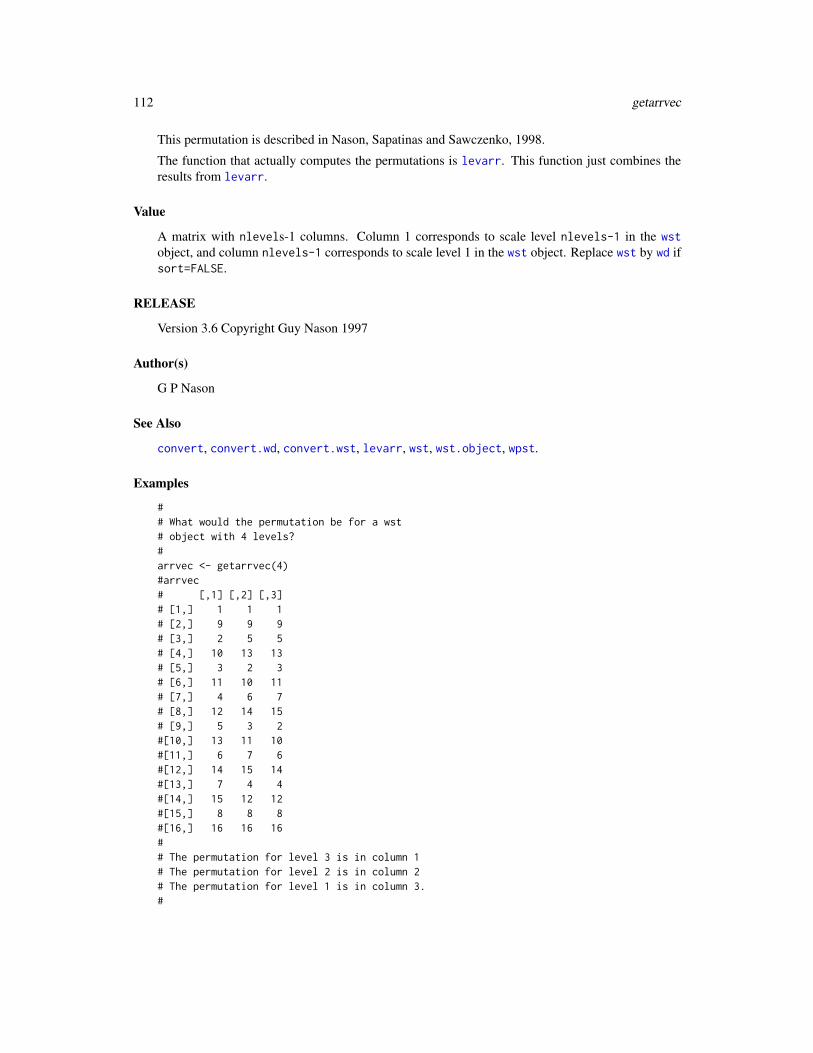
112 getarrvec

This permutation is described in Nason, Sapatinas and Sawczenko, 1998.

The function that actually computes the permutations is levarr. This function just combines theresults from levarr.

Value

A matrix with nlevels-1 columns. Column 1 corresponds to scale level nlevels-1 in the wstobject, and column nlevels-1 corresponds to scale level 1 in the wst object. Replace wst by wd ifsort=FALSE.

RELEASE


Author(s)

G P Nason

See Also

convert, convert.wd, convert.wst, levarr, wst, wst.object, wpst.

Examples

## What would the permutation be for a wst# object with 4 levels?#arrvec <- getarrvec(4)#arrvec# [,1] [,2] [,3]# [1,] 1 1 1# [2,] 9 9 9# [3,] 2 5 5# [4,] 10 13 13# [5,] 3 2 3# [6,] 11 10 11# [7,] 4 6 7# [8,] 12 14 15# [9,] 5 3 2#[10,] 13 11 10#[11,] 6 7 6#[12,] 14 15 14#[13,] 7 4 4#[14,] 15 12 12#[15,] 8 8 8#[16,] 16 16 16## The permutation for level 3 is in column 1# The permutation for level 2 is in column 2# The permutation for level 1 is in column 3.#

getpacket 113

# The following shows that the above is the right permutation (for level 2# at least.## Start off with some random normal data!#myrand <- rnorm(1:16)## Now take both the time ordered non-decimated wavelet# transform and the packet ordered non-decimated wavelet# transform.#myrwdS <- wd(myrand, type="station")myrwst <- wst(myrand)## Let's look at the level 2 coefficients of myrwdS#accessD(myrwdS, level=2)# [1] -0.73280829 -0.97892279 1.33305777 1.46320165 -0.94790098# [6] -1.39276215 0.40023757 0.82517249 -0.56317955 -0.89408713#[11] 0.77166463 1.56204870 -0.34342230 -1.64133182 0.08235115#[16] 1.05668106## Let's look at the level 2 coefficients of myrwst#accessD(myrwst, level=2)# [1] -0.73280829 -0.94790098 -0.56317955 -0.34342230 1.33305777# [6] 0.40023757 0.77166463 0.08235115 -0.97892279 -1.39276215#[11] -0.89408713 -1.64133182 1.46320165 0.82517249 1.56204870#[16] 1.05668106## O.k. So the coefficients are the same, but they are not in the# same order as in myrwdS. So let's use the permutation in the# second column of arrvec to reorder the myrwst coefficients# to have the same order as the myrwdS ones#accessD(myrwst, level=2)[arrvec[,2]]# [1] -0.73280829 -0.97892279 1.33305777 1.46320165 -0.94790098# [6] -1.39276215 0.40023757 0.82517249 -0.56317955 -0.89408713#[11] 0.77166463 1.56204870 -0.34342230 -1.64133182 0.08235115#[16] 1.05668106## These coefficients have the correct ordering.

getpacket Get a packet of coefficients from a wavelet object

Description

This generic function extracts packets of coefficients from various types of wavelet objects.


114 getpacket.wp


wp use the getpacket.wp method.

wst use the getpacket.wst method.

wpst use the getpacket.wpst method.


Use the accessC and accessD function to extract whole resolution levels of coefficients simultane-ously.

Usage

getpacket(...)

Arguments


Value

The packet of coefficients requested.

RELEASE


Author(s)

G P Nason

See Also

getpacket.wp, getpacket.wst, getpacket.wpst, accessD, accessC.

getpacket.wp Get packet of coefficients from a wavelet packet object (wp).

Description

This function extracts and returns a packet of coefficients from a wavelet packet (wp) object.

Usage

## S3 method for class 'wp'getpacket(wp, level, index, ... )

getpacket.wp 115

Arguments

wp Wavelet packet object from which you wish to extract the packet from.

level The resolution level of the coefficients that you wish to extract.

index The index number within the resolution level of the packet of coefficients thatyou wish to extract.


Details

The wp produces a wavelet packet object. The coefficients in this structure can be organised into abinary tree with each node in the tree containing a packet of coefficients.

Each packet of coefficients is obtained by chaining together the effect of the two packet opera-tors DG and DH: these are the high and low pass quadrature mirror filters of the Mallat pyramidalgorithm scheme followed by decimation (see Mallat~(1989b)).

Starting with data cJ at resolution level J containing 2J data points the wavelet packet algorithmoperates as follows. First DG and DH are applied to cJ producing dJ−1 and cJ−1 respectively.Each of these sets of coefficients is of length one half of the original data: i.e. 2J−1. Each of thesesets of coefficients is a set of wavelet packet coefficients. The algorithm then applies both DG andDH to both dJ−1 and cJ−1 to form a four sets of coefficients at level J-2. Both operators are usedagain on the four sets to produce 8 sets, then again on the 8 sets to form 16 sets and so on. At levelj=J,...,0 there are 2J−j packets of coefficients each containing 2j coefficients.

This function enables whole packets of coefficients to be extracted at any resolution level. Theindex argument chooses a particular packet within each level and thus ranges from 0 (which alwaysrefer to the father wavelet coefficients), 1 (which always refer to the mother wavelet coefficients)up to 2J−j .

Value

A vector containing the packet of wavelet packet coefficients that you wished to extract.

RELEASE


Author(s)

G P Nason

See Also

wp, putpacket.wp, basisplot.wp, draw.wp, InvBasis.wp, MaNoVe.wp, nlevelsWT.wp, plot.wp.threshold.wp.

116 getpacket.wpst

Examples

## Take the wavelet packet transform of some random data#MyWP <- wp(rnorm(1:512))## The above data set was 2^9 in length. Therefore there are# coefficients at resolution levels 0, 1, 2, ..., and 8.## The high resolution coefficients are at level 8.# There should be 256 DG coefficients and 256 DH coefficients#length(getpacket(MyWP, level=8, index=0))#[1] 256length(getpacket(MyWP, level=8, index=1))#[1] 256## The next command shows that there are only two packets at level 8### Not run: getpacket(MyWP, level=8, index=2)#Index was too high, maximum for this level is 1#Error in getpacket.wp(MyWP, level = 8, index = 2): Error occured#Dumped## There should be 4 coefficients at resolution level 2## The father wavelet coefficients are (index=0)getpacket(MyWP, level=2, index=0)#[1] -0.9736576 0.5579501 0.3100629 -0.3834068## The mother wavelet coefficients are (index=1)##[1] 0.72871405 0.04356728 -0.43175307 1.77291483## There will be 127 packets at this level.#

getpacket.wpst Get packet of coefficients from a non-decimated wavelet packet object(wpst).

Description

This function extracts and returns a packet of coefficients from a non-decimated wavelet packet(wpst) object.

Usage

## S3 method for class 'wpst'getpacket(wpst, level, index, ... )

getpacket.wpst 117

Arguments

wpst Non-decimated wavelet packet object from which you wish to extract the packetfrom.

level The resolution level of the coefficients that you wish to extract. Can range from0 to nlevelsWT(wpst). The coefficients at level nlevels are the data the createdthe wpst.object.

index The index number within the resolution level of the packet of coefficients thatyou wish to extract. Index ranges from 0 to (4r)−1 where r = nlevelsWT - level.


Details

The wpst transform produces a non-decimated wavelet packet object. This is a "cross" betweena wavelet packet object and a non-decimated wavelet object. In other words the transformproduces wavelet packet coefficients at every possible integer shift (unlike the ordinary waveletpacket transform which is aligned to a dyadic grid).

Each packet of coefficients is obtained by chaining together the effect of the two packet operatorsDG and DH: these are the high and low pass quadrature mirror filters of the Mallat pyramid algo-rithm scheme followed by both even and odd decimation. For a full description of this algorithmand how coefficients are stored within see Nason, Sapatinas and Sawczenko, 1998.

Note that this function extracts packets. If you want to obtain the wavelet packet coefficients foreach shift you need to use the accessD.wpstfunction. This function extracts particular waveletpacket coefficients for a particular shift. In particular, this function returns a number of coeffi-cients dependent on the scale level requested whereas accessD.wpst always returns a vector ofcoefficients of length equal to the input data that created the wpst.object initially.

Value

A vector containing the packet of non-decimated wavelet packet coefficients that you wished toextract.

RELEASE


Author(s)

G P Nason

See Also

accessD.wpst, wpst,

118 getpacket.wst

Examples

## Create some random data#myrand <- rnorm(16)#myrand# [1] 0.19268626 -0.41737181 -0.30806613 0.07435407 0.99871757# [6] -0.58935121 -1.38049759 -0.13346631 1.55555403 -1.60581265#[11] 0.14353621 1.21277774 1.13762337 -1.08577934 -0.29745609#[16] 0.50977512## Do the non-decimated wavelet packet transform#myrwpst <- wpst(myrand)## Let's access what is a level nlevelsWT(myrwpst)#getpacket(myrwpst, nlevelsWT(myrwpst), index=0)# [1] 0.19268626 -0.41737181 -0.30806613 0.07435407 0.99871757# [6] -0.58935121 -1.38049759 -0.13346631 1.55555403 -1.60581265#[11] 0.14353621 1.21277774 1.13762337 -1.08577934 -0.29745609#[16] 0.50977512## I.e. the data that created the object.## How about extracting the 3rd (last) packet at level 3?#getpacket(myrwpst, 3, index=3)#[1] -2.660657144 0.688415755 -1.764060698 0.717267105 -0.206916242#[6] -0.659983747 0.005836952 -0.196874007## Of course, there are only 8 coefficients at this level.

getpacket.wst Get packet of coefficients from a packet ordered non-decimatedwavelet object (wst).

Description

This function extracts and returns a packet of coefficients from a packet-ordered non-decimatedwavelet object (wst) object. The wst objects are computed by the wst function amongst others.

Usage

## S3 method for class 'wst'getpacket(wst, level, index, type="D", aspect, ...)

getpacket.wst 119

Arguments

wst Packet-ordered non-decimated wavelet object from which you wish to extractthe packet from.

level The resolution level of the coefficients that you wish to extract.

index The index number within the resolution level of the packet of coefficients thatyou wish to extract.

type This argument must be either "C" or "D". If the argument is "C" then non-decimated father wavelet coefficients corresponding to the packet that you wantare returned. If the argument is "D" then non-decimated mother wavelet coeffi-cients are returned.

aspect Function applied to the coefficients before return. This is suppled as a characterstring which gets converted to a function to apply. For example, "Mod" forcomplex-valued coefficients returns the absolute values.

... Other arguments

Details

The wst function produces a packet-ordered non-decimated wavelet object: wst. The coefficientsin this structure can be organised into a binary tree with each node in the tree containing a packetof coefficients.

Each packet is obtained by repeated application of the usual DG quadrature mirror filter with botheven and odd dyadic decimation. See the detailed description given in Nason and Silverman, 1995.

This function enables whole packets of coefficients to be extracted at any resolution level. Theindex argument chooses a particular packet within each level and thus ranges from 0 to 2J−j forj=0,..., J-1. Each packet corresponds to the wavelet coefficients with respect to different origins.

Note that both mother and father wavelet coefficient at different shifts are available by using thetype argument.

Value

A vector containing the packet of packet-ordered non-decimated wavelet coefficients that you wishedto extract.

RELEASE


Author(s)

G P Nason

See Also

wst, wst.object,

120 getpacket.wst2D

Examples

## Take the packet-ordered non-decimated transform of some random data#MyWST <- wst(rnorm(1:512))## The above data set was 2^9 in length. Therefore there are# coefficients at resolution levels 0, 1, 2, ..., and 8.## The high resolution coefficients are at level 8.# There should be 256 coefficients at level 8 in index location 0 and 1.#length(getpacket(MyWST, level=8, index=0))#[1] 256length(getpacket(MyWST, level=8, index=1))#[1] 256## There are also 256 FATHER wavelet coefficients at each of these two indices# (origins)#length(getpacket(MyWST, level=8, index=0, type="C"))#[1] 256length(getpacket(MyWST, level=8, index=1, type="C"))#[1] 256## There should be 4 coefficients at resolution level 2#getpacket(MyWST, level=2, index=0)#[1] -0.92103095 0.70125471 0.07361174 -0.43467375## Here are the equivalent father wavelet coefficients#getpacket(MyWST, level=2, index=0, type="C")#[1] -1.8233506 -0.2550734 1.9613138 1.2391913

getpacket.wst2D Get packet of coefficients from a two-dimensional non-decimatedwavelet object (wst2D).

Description

This function extracts and returns a packet of coefficients from a two-dimensional non-decimatedwavelet (wst2D) object.

Usage

## S3 method for class 'wst2D'getpacket(wst2D, level, index, type="S", Ccode=TRUE, ...)

getpacket.wst2D 121

Arguments

wst2D 2D non-decimated wavelet object from which you wish to extract a packet from.

level The resolution level of the coefficients that you wish to extract. Can range from0 to nlevelsWT(wpst)-1.

index The index number within the resolution level of the packet of coefficients thatyou wish to extract. Index is a base-4 number which is r digits long. Each digitcan be 0, 1, 2 or 3 corresponding to no shifts, horizontal shift, vertical shift orhorizontal and vertical shifts. The number r indicates the depth of the resolutionlevel from the data resolution i.e. where r = nlevelsWT - level.Where there is a string of more than one digit the left most digits correspond tofinest scale shift selection, the right most digits to the coarser scales (I think).

type This is a one letter character string: one of "S", "H", "V" or "D" for the smoothcoefficients, horizontal, vertical or diagonal detail.

Ccode If T then fast C code is used to obtain the packet, otherwise slow SPlus code isused. Unless you have some special reason always use the C code (and leave theargument at its default).


Details

The wst2D function creates a wst2D class object. Starting with a smooth the operators H, G, GSand HS (where G, H are the usual Mallat operators and S is the shift-by-one operator) are operatedfirst on the rows and then the columns: i.e. so each of the operators HH, HG, GH, GG, HSH, HSG,GSH, GSG HHS, GHS, HGS, GGS HSHS, HSGS, GSHS and GSGS are applied. Then the samecollection of operators is applied to all the derived smooths, i.e. HH, HSH, HHS and HSHS.

So the next level is obtained from the previous level with basically HH, HG, GH and GG but withextra shifts in the horizontal, vertical and horizontal and vertical directions. The index provides away to enumerate the paths through this tree where each smooth has 4 children and indexed by anumber between 0 and 3.

Each of the 4 children has 4 components: a smooth, horizontal, vertical and diagonal detail, muchin the same way as for the Mallat 2D wavelet transform implemented in the WaveThresh functionimwd.

Value

A matrix containing the packet of the 2D non-decimated wavelet coefficients that you require.

RELEASE


Author(s)

G P Nason

122 getpacket.wst2D

See Also

putpacket.wst2D, wst2D, wst2D.object.

Examples

## Create a random image.#myrand <- matrix(rnorm(16), nrow=4, ncol=4)#myrand# [,1] [,2] [,3] [,4]#[1,] 0.01692807 0.1400891 -0.38225727 0.3372708#[2,] -0.79799841 -0.3306080 1.59789958 -1.0606204#[3,] 0.29151629 -0.2028172 -0.02346776 0.5833292#[4,] -2.21505532 -0.3591296 -0.39354119 0.6147043## Do the 2D non-decimated wavelet transform#myrwst2D <- wst2D(myrand)## Let's access the finest scale detail, not shifted in the vertical# direction.#getpacket(myrwst2D, nlevelsWT(myrwst2D)-1, index=0, type="V")# [,1] [,2]#[1,] -0.1626819 -1.3244064## Compare this to the ordinary 2D DWT for the vertical detail at this# resolution levelimwd(myrand)[[lt.to.name( 1, "DC")]]#[1] -0.1626819 -1.3244064 1.4113247 -0.7383336## The same numbers but they're not in matrix format because# imwd returns vectors not matrices.## Now back to the wst2D object. Let's# extract vertical detail again at level 1 but this time the horizontally# shifted data.#getpacket(myrwst2D, level=1, index=1, type="V")# [,1] [,2]#[1,] -0.5984427 0.2599445#[2,] -0.6502002 1.8027955## So, yes, different data. Now how about at a deeper resolution level.# Lets have a horizontal shift, as before, for the level 1 but follow it# with a diagonal shift and this time extract the smooth component:#getpacket(myrwst2D, level=0, index=13, type="S")# [,1]#[1,] -0.5459394#

GetRSSWST 123

# Of course, only one number because this is at level 0

GetRSSWST Computes estimate of error for function estimate.

Description

Computes estimate of error for function estimate. Given noisy data and a threshold value thisfunction uses Nason’s 1996 two-fold cross-validation algorithm, but using packet ordered non-decimated wavelet transforms to compute two estimates of an underlying “true” function and usesthem to compute an estimate of the error in estimating the truth.

Usage

GetRSSWST(ndata, threshold, levels, family = "DaubLeAsymm",filter.number = 10, type = "soft", norm = l2norm, verbose = 0,InverseType = "average")

Arguments

ndata the noisy data. This is a vector containing the signal plus noise. The length ofthis vector should be a power of two.

threshold the value of the threshold that you wish to compute the error of the estimate at

levels the levels over which you wish the threshold value to be computed (the thresh-old that is used in computing the estimate and error in the estimate). See theexplanation for this argument in the threshold.wst function.



type whether to use hard or soft thresholding. See the explanation for this argumentin the threshold.wst function.

norm which measure of distance to judge the dissimilarity between the estimates. Thefunctions l2norm and linfnorm are suitable examples.

verbose If TRUE then informative messages are printed during the progression of thefunction, otherwise they are not.

InverseType The possible options are "average" or "minent". The former uses basis averagingto form estimates of the unknown function. The "minent" function selects a basisusing the Coifman and Wickerhauser, 1992 algorithm to select a basis to invert.

124 griddata objects

Details

This function implements the component of the cross-validation method detailed by Nason, 1996 forcomputing an estimate of the error between an estimate and the “truth”. The difference here is that ituses the packet ordered non-decimated wavelet transform rather than the standard Mallat wd discretewavelet transform. As such it is an examples of the translation-invariant denoising of Coifman andDonoho, 1995 but uses cross-validation to choose the threshold rather than SUREshrink.

Note that the procedure outlined above can use AvBasis basis averaging or basis selection andinversion using the Coifman and Wickerhauser, 1992 best-basis algorithm

Value

A real number which is estimate of the error between estimate and truth at the given threshold.

RELEASE


Author(s)

G P Nason

See Also

linfnorm, linfnorm, wstCV, wstCVl.

Examples

## This function performs the error estimation step for the# \code{\link{wstCV}} function and so is not intended for# user use.#

griddata objects Data interpolated to a grid objects.

Description

These are objects of classes

griddata

These objects store the results of interpolating a 1-D regression data set to a grid which is a powerof two in length

griddata objects 125

Details

The help page for makegrid and Kovac, (1997), p.81 give further details about how a griddataobject is constructed.

Value

The following components must be included in a legitimate griddata object.

gridt a vector containing the values of the grid on the "x" axis.

gridy a vector containing the values of the grid on the "y" axis. This vector has to bethe same length as gridt. Typically the values in (gridt, gridy) are the resultsof interpolating arbitrary data (x,y) onto (gridt, gridy).

GCodes the value of the linear interpolant matrix for the corresponding entry in gridt. The valueat each point corresponds to the proportion of the original data point pointed to by Gindex thatcontributes to the new value at the corresponding gridt value. See Kovac, (1997), page 81 forfurther information.

Gindex Each entry in Gindex refers to one of the pairs in (x,y) which is contributing tothe (gridt, gridy) interpolant. See previous help for G.

GENERATION

This class of objects is returned from the makegrid function to represent the results of interpolatinga 1-D regression data set to a grid.

METHODS

The griddata class of objects really on has one function that uses it: irregwd.

RELEASE

Version 3.9.6 Copyright Arne Kovac 1997 Copyright Guy Nason (help pages) 1999.

SEE ALSO

makegrid, irregwd

Author(s)

Arne Kovac

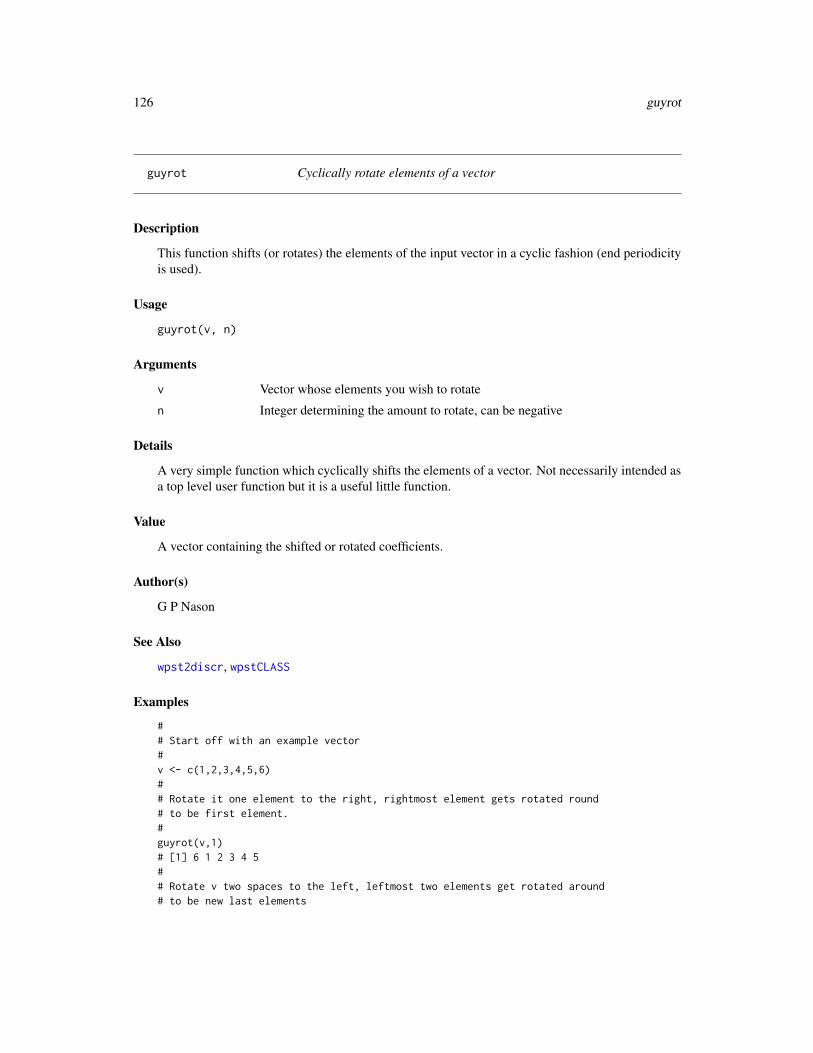
126 guyrot

guyrot Cyclically rotate elements of a vector

Description

This function shifts (or rotates) the elements of the input vector in a cyclic fashion (end periodicityis used).

Usage

guyrot(v, n)

Arguments

v Vector whose elements you wish to rotate

n Integer determining the amount to rotate, can be negative

Details

A very simple function which cyclically shifts the elements of a vector. Not necessarily intended asa top level user function but it is a useful little function.

Value

A vector containing the shifted or rotated coefficients.

Author(s)

G P Nason

See Also

wpst2discr, wpstCLASS

Examples

## Start off with an example vector#v <- c(1,2,3,4,5,6)## Rotate it one element to the right, rightmost element gets rotated round# to be first element.#guyrot(v,1)# [1] 6 1 2 3 4 5## Rotate v two spaces to the left, leftmost two elements get rotated around# to be new last elements

HaarConcat 127

guyrot(v, -2)## [1] 3 4 5 6 1 2### Now issue a larger rotation, e.g. 19!#guyrot(v,19)# [1] 6 1 2 3 4 5## Its just the same as rotating by 1 since the input vector is of length 6# and so rotating by 19 is the same as rotating by 6,6,6, and then 1!#

HaarConcat Generate a concatenated Haar MA process

Description

This function generates a particular set of four concatenated Haar MA processes.

Usage

HaarConcat()

Arguments

None

Details

This function generates a realization of particular kind of non-stationary time series probabilitymodel. The returned time series is the result of concatenating 4 time series each of length 128from the Haar MA process generator (HaarMA) of orders 1, 2, 3 and 4. The standard deviation ofthe innovations is 1. This function was used to generate the figure of the concatenated Haar MAprocess in Nason, von Sachs and Kroisandt. It produces a kind of time series that can be sparselyrepresented by the wavelet machinery but at the same time is non-stationary.

See Nason, von Sachs and Kroisandt (2000) Wavelet processes and adaptive estimation of the evo-lutionary wavelet spectrum. J R Statist Soc, B, 62, 271-292.

Value

A vector containing 512 observations from four concatenated Haar MA processes

Author(s)

G P Nason

128 HaarMA

See Also

HaarMA,ewspec

Examples

## Generate the concatenated Haar MA process.#MyHaarCC <- HaarConcat()## Plot it### Not run: ts.plot(MyHaarCC)

HaarMA Generate Haar MA processes.

Description

This function generates an arbitrary number of observations from a Haar MA process of any orderwith a particular variance.

Usage

HaarMA(n, sd=1, order=5)

Arguments

n The number of observations in the realization that you want to create. Note thatn does NOT have to be a power of two.

sd The standard deviation of the innovations.order The order of the Haar MA process.

Details

A Haar MA process is a special kind of time series moving-average (MA) process. A Haar MAprocess of order k is a MA process of order 2k. The coefficients of the Haar MA process are givenby the filter coefficients of the discrete Haar wavelet at different scales.

For examples: the Haar MA process of order 1 is an MA process of order 2. The coefficients are1/√2 and −1/

√2. The Haar MA process of order 2 is an MA process of order 4. The coefficients

are 1/2, 1/2, -1/2, -1/2 and so on. It is possible to define other processes for other wavelets as well.

Any Haar MA process is a good examples of a (stationary) LSW process because it is sparsely rep-resentable by the locally-stationary wavelet machinery defined in Nason, von Sachs and Kroisandt.

Value

A vector containing a realization of a Haar MA process of the specified order, standard deviationand number of observations.

HaarMA 129

RELEASE


Author(s)

G P Nason

References


See Also

HaarConcat, ewspec,

Examples

## Generate a Haar MA process of order 1 (high frequency series)#MyHaarMA <- HaarMA(n=151, sd=2, order=1)## Plot it### Not run: ts.plot(MyHaarMA)## Generate another Haar MA process of order 3 (lower frequency), but of# smaller variance#MyHaarMA2 <- HaarMA(n=151, sd=1, order=3)## Plot it### Not run: ts.plot(MyHaarMA2)## Let's plot them next to each other so that you can really see the# differences.## Plot a vertical dotted line which indicates where the processes are# joined### Not run: ts.plot(c(MyHaarMA, MyHaarMA2))## Not run: abline(v=152, lty=2)

130 image.wd

image.wd Produce image representation of nondecimated wavelet transform

Description

Produces a representation of a nondecimated wavelet transform (time-ordered) as an image.

Usage

## S3 method for class 'wd'image(x, strut = 10, type = "D", transform = I, ...)

Arguments

x The wd.object that you wish to image

strut The width of each coefficient in the image

type Either "C" or "D" depending if you wish to image scaling function or waveletcoefficients respectively

transform Apply a numerical transform to the coefficients before display

... Other arguments

Details


Value

None

Author(s)

G P Nason

See Also

logabs, nlevelsWT,wd

Examples

tmp <- wd(rnorm(256), type="station")## Not run: image(tmp)

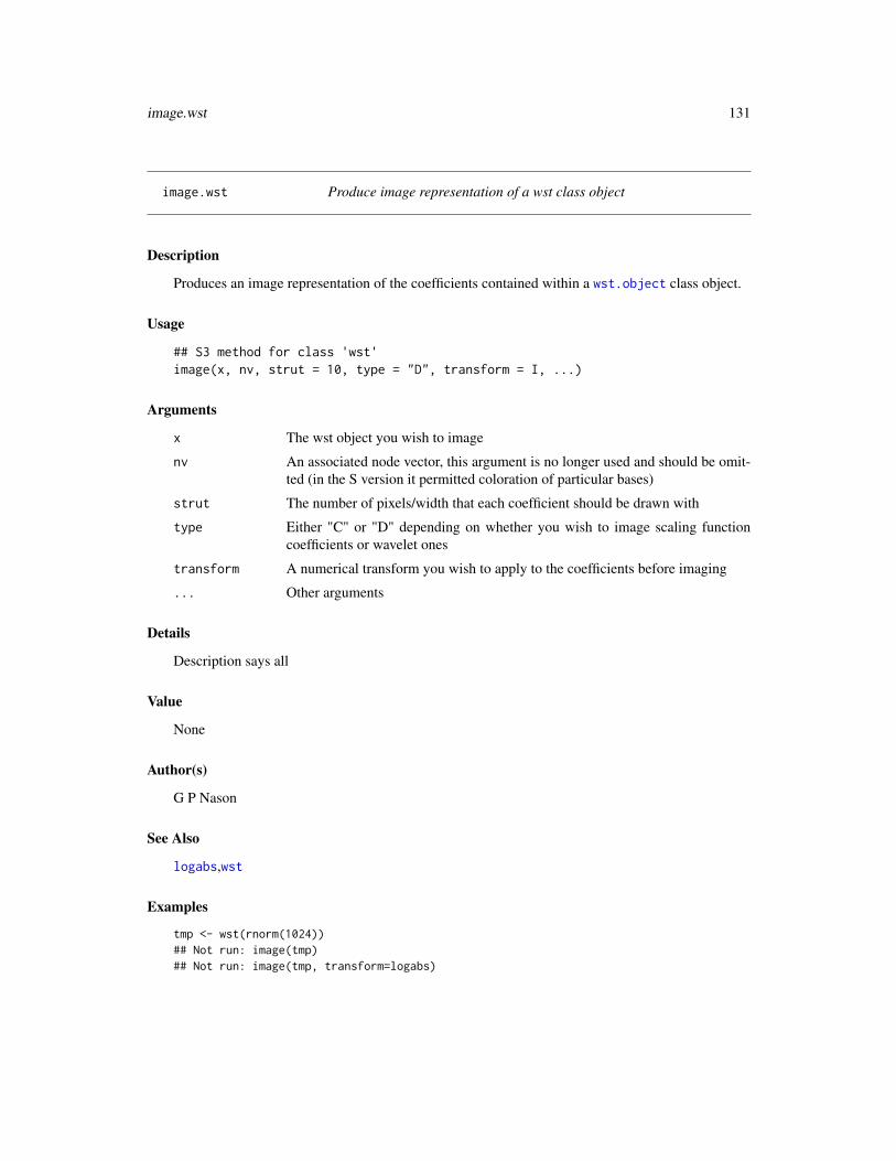
image.wst 131

image.wst Produce image representation of a wst class object

Description

Produces an image representation of the coefficients contained within a wst.object class object.

Usage

## S3 method for class 'wst'image(x, nv, strut = 10, type = "D", transform = I, ...)

Arguments

x The wst object you wish to image

nv An associated node vector, this argument is no longer used and should be omit-ted (in the S version it permitted coloration of particular bases)

strut The number of pixels/width that each coefficient should be drawn with

type Either "C" or "D" depending on whether you wish to image scaling functioncoefficients or wavelet ones

transform A numerical transform you wish to apply to the coefficients before imaging

... Other arguments

Details


Value

None

Author(s)

G P Nason

See Also

logabs,wst

Examples

tmp <- wst(rnorm(1024))## Not run: image(tmp)## Not run: image(tmp, transform=logabs)

132 imwd

imwd Two-dimensional wavelet transform (decomposition).

Description

This function can perform two types of two-dimensional discrete wavelet transform (DWT). Thestandard transform (type="wavelet") computes the 2D DWT according to Mallat’s pyramidal al-gorithm (Mallat, 1989). The spatially ordered non-decimated 2D DWT (NDWT) (type="station")contains all possible spatially shifted versions of the DWT. The order of computation of the DWTis O(n), and it is O(n log n) for the NDWT if n is the number of pixels.

Usage

imwd(image, filter.number=10, family="DaubLeAsymm", type="wavelet",bc="periodic", RetFather=TRUE, verbose=FALSE)

Arguments

image A square matrix containing the image data you wish to decompose. The side-length of this matrix must be a power of 2.



type specifies the type of wavelet transform. This can be "wavelet" (default) in whichcase the standard 2D DWT is performed (as in previous releases of WaveThresh).If type is "station" then the 2D spatially-ordered non-decimated DWT is per-formed. At present, only periodic boundary conditions can be used with the 2Dspatially ordered non-decimated wavelet transform.

bc specifies the boundary handling. If bc=="periodic" the default, then the func-tion you decompose is assumed to be periodic on it’s interval of definition, ifbc=="symmetric" then the function beyond its boundaries is assumed to be asymmetric reflection of the function in the boundary. The symmetric option wasthe implicit default in releases prior to 2.2. Note that only periodic boundaryconditions are valid for the 2D spatially-ordered non-decimated wavelet trans-form.

RetFather If TRUE then this argument causes the scaling function coefficients at each reso-lution level to be returned as well as the wavelet coefficients. If FALSE then noscaling function coefficients are returned. The opportunity of returning fatherwavelet coefficients has been added since previous versions of WaveThresh.


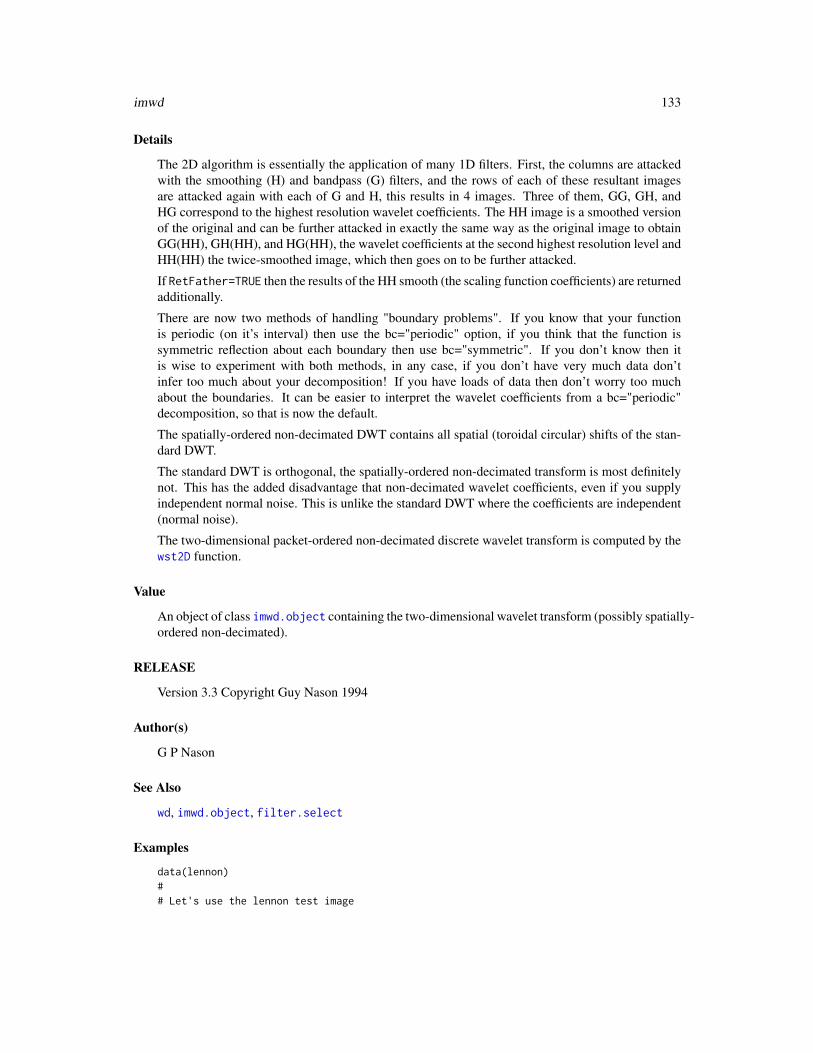
imwd 133

Details

The 2D algorithm is essentially the application of many 1D filters. First, the columns are attackedwith the smoothing (H) and bandpass (G) filters, and the rows of each of these resultant imagesare attacked again with each of G and H, this results in 4 images. Three of them, GG, GH, andHG correspond to the highest resolution wavelet coefficients. The HH image is a smoothed versionof the original and can be further attacked in exactly the same way as the original image to obtainGG(HH), GH(HH), and HG(HH), the wavelet coefficients at the second highest resolution level andHH(HH) the twice-smoothed image, which then goes on to be further attacked.

If RetFather=TRUE then the results of the HH smooth (the scaling function coefficients) are returnedadditionally.

There are now two methods of handling "boundary problems". If you know that your functionis periodic (on it’s interval) then use the bc="periodic" option, if you think that the function issymmetric reflection about each boundary then use bc="symmetric". If you don’t know then itis wise to experiment with both methods, in any case, if you don’t have very much data don’tinfer too much about your decomposition! If you have loads of data then don’t worry too muchabout the boundaries. It can be easier to interpret the wavelet coefficients from a bc="periodic"decomposition, so that is now the default.

The spatially-ordered non-decimated DWT contains all spatial (toroidal circular) shifts of the stan-dard DWT.

The standard DWT is orthogonal, the spatially-ordered non-decimated transform is most definitelynot. This has the added disadvantage that non-decimated wavelet coefficients, even if you supplyindependent normal noise. This is unlike the standard DWT where the coefficients are independent(normal noise).

The two-dimensional packet-ordered non-decimated discrete wavelet transform is computed by thewst2D function.

Value

An object of class imwd.object containing the two-dimensional wavelet transform (possibly spatially-ordered non-decimated).

RELEASE


Author(s)

G P Nason

See Also

wd, imwd.object, filter.select

Examples

data(lennon)## Let's use the lennon test image

134 imwd.object

### Not run: image(lennon)## Now let's do the 2D discrete wavelet transform#lwd <- imwd(lennon)## Let's look at the coefficients### Not run: plot(lwd)

imwd.object Two-dimensional wavelet decomposition objects.

Description


imwd

They represent a decomposition of an image with respect to a two-dimensional wavelet basis (ortight frame in the case of the two-dimensional (space-ordered) non-decimated wavelet decomposi-tion).

Details

In previous releases the original image was stored as the "original" component of a imwd object.This is not done now as the resulting objects were excessively large.

Value

The following components must be included in a legitimate ‘imwd’ object.

nlevelsWT number of levels in wavelet decomposition. If you raise 2 to the power of nlevelsthen you get the dimension of the image that you originally started with.

type If type="wavelet" then the image was decomposed according to the 2D Mallatpyramidal algorithm. If type="station" then the image was decomposed usingthe 2D spatially ordered non-decimated wavelet transform.

fl.dbase The first last database associated with the decomposition. For images, this list isnot very useful as each level’s components is stored as a list component, ratherthan being packaged up in a single vector as in the 1D case. Nevertheless theinternals still need to know about fl.dbase to get the computations correct. Seethe help for first.last if you are a masochist.

filter A filter object as returned by the filter.select function. This componentrecords the filter used in the decomposition. The reconstruction routines usethis component to find out what filter to use in reconstruction.

imwdc.object 135

wNLx The object will probably contain many components with names of this form.These are all the wavelet coefficients of the decomposition. In "wNLx" the "N"refers to the level number and the "x" refers to the direction of the coefficientswith "1" being horizontal, "2" being vertical and "3" being diagonal and "4"corresonding to scaling function coefficients at the given resolution level. Notethat the levels should be in numerically decreasing order, so if nlevelsWT is 5,then there will be w5L1, w5L2, w5L3 first, then down to w1L1, w1L2, andw1L3. Note that these coefficients store their data according to the first.lastdatabase fl.dbase$first.last.d, so refer to them using this. Note that iftype="wavelet" then images at level N are subimages of side length 2^N pixels.If the type component is "station" then each coefficient subimage is of thesame dimension as the input image used to create this object.

w0Lconstant This is the coefficient of the bottom level scaling function coefficient. So forexamples, if you used Haar wavelets this would be the sample mean of the data(scaled by some factor depending on the number of levels, nlevelsWT).

bc This component details how the boundaries were treated in the decomposition.

GENERATION

This class of objects is returned from the imwd function to represent a two-dimensional (possiblyspace-ordered non-decimated) wavelet decomposition of a function. Many other functions returnan object of class imwd.

METHODS

The imwd class of objects has methods for the following generic functions: compress, draw, imwr,nullevels.imwd, plot, print, summary, threshold.imwd.

RELEASE


Author(s)

G P Nason

See Also

imwd

imwdc.object Two-dimensional compressed wavelet decomposition objects.

Description


imwdc

They represent a decomposition of an image with respect to a two-dimensional wavelet basis

136 imwdc.object

Details

In previous releases the original image was stored as the "original" component of a imwd object.This is not done now as the resulting objects were excessively large.

To uncompress this class of object back into an object of class imwd.object use the uncompress.imwdcfunction.

Value

The following components must be included in a legitimate ‘imwdc’ object.

nlevelsWT number of levels in wavelet decomposition. If you raise 2 to the power of nlevelsthen you get the dimension of the image that you originally started with.

type If type="wavelet" then the image was decomposed according to the 2D Mallatpyramidal algorithm. If type="station" then the image was decomposed usingthe 2D spatially ordered non-decimated wavelet transform.

fl.dbase The first last database associated with the decomposition. For images, this list isnot very useful as each level’s components is stored as a list component, ratherthan being packaged up in a single vector as in the 1D case. Nevertheless theinternals still need to know about fl.dbase to get the computations correct. Seethe help for first.last if you are a masochist.

filter A filter object as returned by the filter.select function. This componentrecords the filter used in the decomposition. The reconstruction routines usethis component to find out what filter to use in reconstruction.

wNLx The object will probably contain many components with names of this form.These are all the wavelet coefficients of the decomposition. In "wNLx" the "N"refers to the level number and the "x" refers to the direction of the coefficientswith "1" being horizontal, "2" being vertical and "3" being diagonal. Note thatimwdc objects do not contain scaling function coefficients. This would negatethe point of having a compressed object.

Each vector stores its coefficients using an object of class compressed, i.e. thevector is run-length encoded on zeroes.

Note that the levels should be in numerically decreasing order, so if nlevelsWTis 5, then there will be w5L1, w5L2, w5L3 first, then down to w1L1, w1L2, andw1L3. Note that these coefficients store their data according to the first.lastdatabase fl.dbase$first.last.d, so refer to them using this.

Note that if type="wavelet" then images at level N are subimages of sidelength 2^N pixels. If the type component is "station" then each coefficientsubimage is of the same dimension as the input image used to create this object.

w0Lconstant This is the coefficient of the bottom level scaling function coefficient. So forexamples, if you used Haar wavelets this would be the sample mean of the data(scaled by some factor depending on the number of levels, nlevelsWT).

bc This component details how the boundaries were treated in the decomposition.

imwdc.object 137

GENERATION

This class of objects is returned from the threshold.imwd function to represent a thresholded two-dimensional wavelet decomposition of a function. Some other functions return an object of classimwdc.

METHODS

The imwd class of objects has methods for the following generic functions: draw, imwr, nullevels,plot, print, summary, threshold.imwdc.

RELEASE


Author(s)

G P Nason

See Also

imwd imwd.object, threshold.imwd, uncompress.imwdc.

Examples

## Perform the standard two-dimensional DWT# on the lennon image.#data(lennon)

lwd <- imwd(lennon)## Now let's see how many horizontal detail coefficients there are at# scale 6#length(lwd$w6L1)# [1] 4096## So the horizontal detail `ìmage'' at scale contains 64x64=4096 coefficients.# A lot!## Now, suppose we threshold this# two-dimensional wavelet decomposition object#lwdT <- threshold(lwd)## First of all. What is the class of the detail coefficients now?#class(lwdT$w6L1)# [1] "compressed"#

138 imwr

# Aha. So this set of coefficients got compressed using the# compress.default function.## How many coefficients are being stored here?#lwdT$w6L1# $position:# [1] 173 2829 2832 2846## $values:# [1] 141.5455 -190.2810 -194.5714 -177.1791## $original.length:# [1] 4096## attr(, "class"):# [1] "compressed"## Wow! Only 4 coefficients are not zero. Wicked compression!

imwr Inverse two-dimensional wavelet transform.

Description

Perform inverse two-dimensional wavelet transform using Mallat’s, 1989 algorithm.


Particular methods exist. For the imwd class object this generic function uses imwr.imwd. For theimwdc class object this generic function uses imwr.imwdc.

Usage

imwr(...)

Arguments


Details


Value

A square matrix whose side length is a power of two that represents the inverse 2D wavelet trans-form of the input object x.

imwr.imwd 139

RELEASE


Author(s)

G P Nason

See Also

imwd, imwr.imwd, imwr.imwdc.

imwr.imwd Inverse two-dimensional discrete wavelet transform.

Description

This functions performs the reconstruction stage of Mallat’s pyramid algorithm (i.e. the inversediscrete wavelet transform) for images.

Usage

## S3 method for class 'imwd'imwr(imwd, bc=imwd$bc, verbose=FALSE, ...)

Arguments

imwd An object of class ‘imwd’. This type of object is returned by ‘imwd’.

bc This argument specifies the boundary handling, it is best left to be the boundaryhandling specified by that in the supplied imwd (as is the default).

verbose If this argument is true then informative messages are printed detailing the com-putations to be performed


Details

Details of the algorithm are to be found in Mallat (1989). Similarly to the decomposition function,imwd the inverse algorithm works by applying many 1D reconstruction algorithms to the coeffi-cients. The filters in these 1D reconstructions are incorporated in the supplied imwd.object andoriginally created by the filter.select function in WaveThresh3.

This function is a method for the generic function imwr for class imwd.object. It can be invokedby calling imwr for an object of the appropriate class, or directly by calling imwr.imwd regardlessof the class of the object.

140 imwr.imwdc

Value

A matrix, of dimension determined by the original data set supplied to the initial decomposition(more precisely, determined by the nlevelsWT component of the imwd.object). This matrix isthe highest resolution level of the reconstruction. If a imwd two-dimensional wavelet transformis followed immediately by a imwr inverse two-dimensional wavelet transform then the returnedmatrix will be exactly the same as the original image.

RELEASE


Author(s)

G P Nason

See Also

imwd, imwd.object, imwr.

Examples

## Do a decomposition, then exact reconstruction# Look at the error#test.image <- matrix(rnorm(32*32), nrow=32)## Test image is just some sort of square matrix whose side length# is a power of two.#max( abs(imwr(imwd(test.image)) - test.image))# [1] 1.014611e-11

imwr.imwdc Inverse two-dimensional discrete wavelet transform.

Description

Inverse two-dimensional discrete wavelet transform.

Usage

## S3 method for class 'imwdc'imwr(imwd, verbose=FALSE, ...)

imwr.imwdc 141

Arguments

imwd An object of class imwdc. This type of object is returned by threshold.imwdand is a compress.imwd compressed version of an imwd object.

verbose If this argument is true then informative messages are printed detailing the com-putations to be performed

... other arguments to supply to the imwr function which is called after uncom-pressing the imwdc object.

Details

This function merely uncompresses the supplied imwdc.object and passes the resultant imwd objectto the imwr.imwd function.

This function is a method for the generic function imwr for class imwdc.object. It can be invokedby calling imwr for an object of the appropriate class, or directly by calling imwr.imwdc regardlessof the class of the object.

Value

A matrix, of dimension determined by the original data set supplied to the initial decomposition(more precisely, determined by the nlevelsWT component of the imwdc.object). This matrix isthe highest resolution level of the reconstruction.

RELEASE


Author(s)

G P Nason

See Also

compress.imwd, imwd, imwd.object, imwr.

Examples

## Do a decomposition, thresholding, then exact reconstruction# Look at the error#

test.image <- matrix(rnorm(32*32), nrow=32)

# Test image is just some sort of square matrix whose side length# is a power of two.#max( abs(imwr(threshold(imwd(test.image))) - test.image))# [1] 62.34#

142 InvBasis

# The answer is not zero (see contrasting examples in the help page for# imwr.imwd because we have thresholded the# 2D wavelet transform here).

InvBasis Generic basis inversion for libraries

Description

Will invert either a wst or wp object given that object and some kind of basis specification.

Usage

InvBasis(...)

Arguments

... Usually a library representation and a basis specification

Details

Description says it all

Value

The reconstruction.

Author(s)

G P Nason

See Also

InvBasis.wp,InvBasis.wst,MaNoVe,numtonv

InvBasis.wp 143

InvBasis.wp Invert a wp library representation with a particular basis spec

Description

Inverts a wp basis representation with a given basis specification, for example an output from theMaNoVe function.

Usage

## S3 method for class 'wp'InvBasis(wp, nvwp, pktlist, verbose=FALSE, ...)

Arguments

wp The wavelet packet object you wish to invert.

nvwp A basis specification in the format of a node vector (wp) object, obtained, eg bythe MaNoVe.wp function

pktlist Another way of specifying the basis. If this argument is not specified then itis generated automatically from the nvwp argument. If it is specified then itoverrides the one generated by nvwp

verbose If TRUE then informative messages are printed.

... Other arguments, not used

Details

Objects arising from a wp.object specification are a representation of a signal with respect to alibrary of wavelet packet basis functions. A particular basis specification can be obtained using thenumtonv function which can pick an indexed basis function, or MaNoVe.wp which uses the Coifman-Wickerhauser minimum entropy method to select a basis. This function takes a wp.object and aparticular basis description (in a nv.object node vector object) and inverts the representation withrespect to that selected basis.

The function can alternatively take a packet list pktlist specification which overrides the nodevector if supplied. If the pktlist is missing then one is generated internally from the nvwp objectusing the print.nvwp function.

Value

The inverted reconstruction

Author(s)

G P Nason

See Also

InvBasis,MaNoVe.wp,numtonv,print.nvwp,wp

144 InvBasis.wst

Examples

## The example in InvBasis.wst can be used here, but replaced wst by wp#

InvBasis.wst Invert a wst library representation with a basis specification

Description

Inverts a wst basis representation with a given basis specification, for example an output from theMaNoVe function.

Usage

## S3 method for class 'wst'InvBasis(wst, nv, ...)

Arguments

wst The wst object that you wish to invert

nv The node vector, basis spec, that you want to pick out

... Other arguments, that don’t do anything here

Details

Objects arising from a wst.object specification are a representation of a signal with respect to a li-brary of basis functions. A particular basis specification can be obtained using the numtonv functionwhich can pick an indexed basis function, or MaNoVe.wst which uses the Coifman-Wickerhauserminimum entropy method to select a basis. This function takes a wst.object and a particular basisdescription (in a nv.object node vector object) and inverts the representation with respect to thatselected basis.

Value

The inverted reconstruction

Author(s)

G P Nason

See Also

numtonv,nv.object,MaNoVe.wst,threshold.wst,wst

ipd 145

Examples

## Let's generate a noisy signal#x <- example.1()$y + rnorm(512, sd=0.2)## You can plot this if you like### Not run: ts.plot(x)## Now take the nondecimated wavelet transform#xwst <- wst(x)## Threshold it#xwstT <- threshold(xwst)## You can plot this too if you like### Not run: plot(xwstT)## Now use Coifman-Wickerhauser to get a "good" basis#xwstTNV <- MaNoVe(xwstT)## Now invert the thresholded wst using this basis specification#xTwr <- InvBasis(xwstT, xwstTNV)## And plot the result, and superimpose the truth in dotted### Not run: ts.plot(xTwr)## Not run: lines(example.1()$y, lty=2)

ipd Inductance plethysmography data.

Description

Inductance plethysmography trace.

Usage

data(ipd)

Author(s)

G P Nason

146 ipndacw

Source

This data set contains 4096 observations of inductance plethsymography data sampled at 50Hzstarting at 1229.98 seconds. This is a regular time series object.

I am grateful to David Moshal and Andrew Black of the Department of Anaesthesia, University ofBristol for permission to include this data set.

This data set was used in Nason, 1996 to illustrate noise reduction with wavelet shrinkage and usingcross-validation for choosing the threshold.

A plethysmograph is an apparatus for measuring variations in the size of parts of the body. In thisexperiment the inductance plethysmograph consists of a coil of wire encapsulated in a belt. A radio-frequency carrier signal is passed through the wire and size variations change the inductance of thecoil that can be detected as a change in voltage. When properly calibrated the output voltage of theinductance plethysmograph is proportional to the change in volume of the part of the body underexamination.

It is of both clinical and scientific interest to discover how anaesthetics or analgesics may alternormal breathing patterns post-operatively. Sensors exist that measure blood oxygen saturation butby the time they indicate critically low levels the patient is often apnoeic (cease breathing) and inconsiderable danger. It is possible for a nurse to continually observe a patient but this is expensive,prone to error and requires training. In this examples the plethysmograph is arranged around thechest and abdomen of a set of patients and is used to measure the flow of air during breathing. Therecordings below were made by the Department of Anaesthesia at the Bristol Royal Infirmary afterthe patients had undergone surgery under general anaesthetic. The data set (shown below) showsa section of plethysmograph recording lasting approximately 80 seconds. The two main sets ofregular oscillations correspond to normal breathing. The disturbed behaviour in the centre of theplot where the normal breathing pattern disappears corresponds to the patient vomiting.

Examples

#data(ipd)## Not run: ts.plot(ipd)

ipndacw Compute inner product matrix of discrete non-decimated autocorrela-tion wavelets.

Description

This function computes the inner product matrix of discrete non-decimated autocorrelation wavelets.

Usage

ipndacw(J, filter.number = 10, family = "DaubLeAsymm", tol = 1e-100, verbose= FALSE, ...)

ipndacw 147

Arguments

J Dimension of inner product matrix required. This number should be a negativeinteger.

filter.number The index of the wavelet used to compute the inner product matrix.

family The family of wavelet used to compute the inner product matrix.

tol In the brute force computation for Daubechies compactly supported waveletsmany inner product computations are performed. This tolerance discounts anyresults which are smaller than tol which effectively defines how long the innerproduct/autocorrelation products are.

verbose If TRUE then informative messages are printed. Some of these can be quite fun asthe function tells you whether precomputed matrices are being used, how muchcomputation needs to be done and so forth.


Details

This function computes the inner product matrix of the discrete non-decimated autocorrelationwavelets. This matrix is used to correct the wavelet periodogram as a step to turning it into aevolutionary wavelet spectral estimate. The matrix returned by ipndacw is the one called A in thepaper by Nason, von Sachs and Kroisandt.

For the Haar wavelet the matrix is computed by using the analytical formulae in the paper by Nason,von Sachs and Kroisandt and is hence very fast and efficient and can be used for large values of -J.

For other Daubechies compactly supported wavelets the matrix is computed directly by autocorre-lating discrete non-decimated wavelets at different scales and then forming the inner products ofthese. A function that computes the autocorrelation wavelets themselves is PsiJ. This brute forcecomputation is slow and memory inefficient hence ipndacw contains a mechanism that stores anyinner product matrix that it creates according to a naming scheme defined by the convention definedin rmname. The stored matrices are assigned to the user-visible environment WTEnv.

These stored matrices can be used in future computations by the following automatic procedure:

1 The rmget looks to see whether previous computations have been performed that might be useful.

2 If a matrix of higher order is discovered then the appropriate top-left submatrix is returned, oth-erwise...

3 If the right order of matrix is found it is returned, otherwise ...

4 If a matrix of smaller order is found it is used as the top-left submatrix of the answer. Theremaining elements to the right of and below the submatrix are computed and then the wholematrix is returned, otherwise...

5 If none are found then the whole matrix is computed in C and returned.

In this way a particular matrix for a given wavelet need only be computed once.

Value

A matrix of order (-J)x(-J) containing the inner product matrix of the discrete non-decimated auto-correlation matrices.

148 ipndacw

RELEASE


Author(s)

G P Nason

References


See Also

ewspec, PsiJ, rmname, rmget, filter.select.

Examples

## Let us create the 4x4 inner product matrix for the Haar wavelet.# We'll turn on the jolly verbose messages as well.#ipndacw(-4, filter.number=1, family="DaubExPhase", verbose=TRUE)#Computing ipndacw#Calling haarmat#Took 0.0699999 seconds# -1 -2 -3 -4#-1 1.5000 0.7500 0.3750 0.1875#-2 0.7500 1.7500 1.1250 0.5625#-3 0.3750 1.1250 2.8750 2.0625#-4 0.1875 0.5625 2.0625 5.4375## If we do this again it will use the precomputed version#ipndacw(-4, filter.number=1, family="DaubExPhase", verbose=TRUE)#Computing ipndacw#Returning precomputed version: using 4#Took 0.08 seconds# -1 -2 -3 -4#-1 1.5000 0.7500 0.3750 0.1875#-2 0.7500 1.7500 1.1250 0.5625#-3 0.3750 1.1250 2.8750 2.0625#-4 0.1875 0.5625 2.0625 5.4375## Let's use a smoother wavelet from the least-asymmetric family# and generate the 6x6 version.#ipndacw(-6, filter.number=10, family="DaubLeAsymm", verbose=TRUE)#Computing ipndacw#Took 0.95 seconds# -1 -2 -3 -4 -5

irregwd 149

#-1 1.839101e+00 3.215934e-01 4.058155e-04 8.460063e-06 4.522125e-08#-2 3.215934e-01 3.035353e+00 6.425188e-01 7.947454e-04 1.683209e-05#-3 4.058155e-04 6.425188e-01 6.070419e+00 1.285038e+00 1.589486e-03#-4 8.460063e-06 7.947454e-04 1.285038e+00 1.214084e+01 2.570075e+00#-5 4.522125e-08 1.683209e-05 1.589486e-03 2.570075e+00 2.428168e+01#-6 5.161675e-10 8.941666e-08 3.366416e-05 3.178972e-03 5.140150e+00# -6#-1 5.161675e-10#-2 8.941666e-08#-3 3.366416e-05#-4 3.178972e-03#-5 5.140150e+00#-6 4.856335e+01#

irregwd Irregular wavelet transform (decomposition).

Description

This function performs the irregular wavelet transform as described in the paper by Kovac andSilverman.

Usage

irregwd(gd, filter.number=2, family="DaubExPhase", bc="periodic", verbose=FALSE)

Arguments

gd A grid structure which is the output of the makegrid function.

filter.number This selects the smoothness of wavelet that you want to use in the decomposi-tion. By default this is 2, the Daubechies extremal phase orthonormal compactlysupported wavelet with 2 vanishing moments.

family specifies the family of wavelets that you want to use. Two popular options are"DaubExPhase" and "DaubLeAsymm" but see the help for filter.select formore possibilities.

bc specifies the boundary handling. If bc="periodic" the default, then the func-tion you decompose is assumed to be periodic on it’s interval of definition, ifbc="symmetric" then the function beyond its boundaries is assumed to be asymmetric reflection of the function in the boundary. The symmetric option wasthe implicit default in releases prior to 2.2.


150 irregwd

Details

If one has irregularly spaced one-dimensional regression data (t,y), say. Then the function makegridinterpolates this to a regular grid and then the standard wavelet transform is used to transform theinterpolated data. However, unlike the standard wavelet denoising set-up the interpolated data, y,values are correlated. Hence the wavelet coefficients of the interpolated will be correlated (evenafter using an orthogonal transform). Hence, in particular, the variance of each wavelet coefficientmay well be different and so this routine also computes those variances using a fast algorithm(related to the two-dimensional wavelet transform).

When thresholding with threshold.irregwd the threshold function makes use of the informationabout the variance of each coefficient to modify the variance locally on a coefficient by coefficientbasis.

Value

An object of class irregwd which is a list with the following components.

C Vector of sets of successively smoothed versions of the interpolated data (seedescription of equivalent component of wd.object for further information.)

D Vector of sets of wavelet coefficients of the interpolated data at different resolu-tion levels. (see description of equivalent component of wd.object for furtherinformation.)

c Vector that aids in calculation of variances of wavelet coefficients (used bythreshold.irregwd).

nlevelsWT The number of resolution levels. This depends on the length of the data vector.If length(data)=2^m, then there will be m resolution levels. This means therewill be m levels of wavelet coefficients (indexed 0,1,2,...,(m-1)), and m+1 levelsof smoothed data (indexed 0,1,2,...,m).

fl.dbase There is more information stored in the C and D than is described above. Inthe decomposition “extra” coefficients are generated that help take care of theboundary effects, this database lists where these start and finish, so the "true"data can be extracted.

filter A list containing information about the filter type: Contains the string "wavelet"or "station" depending on which type of transform was performed.

bc How the boundaries were handled.date The date the transform was performed.

RELESASE

3.9.4 Code Copyright Arne Kovac 1997

Author(s)

Arne Kovac

See Also

makegrid, wd, wr.wd, accessC, accessc, accessD, putD, putC, filter.select, plot.irregwd,threshold.irregwd.

irregwd.objects 151

Examples

## See full examples at the end of the help for makegrid.#

irregwd.objects Irregular wavelet decomposition objects.

Description


wd

They represent a decomposition of a function with respect to a wavelet basis. The function willhave been interpolated to a grid and these objects represent the discrete wavelet transform wd.

Details

To retain your sanity the C and D coefficients should be extracted by the accessC and accessDfunctions and inserted using the putC and putD functions (or more likely, their methods), ratherthan by the $ operator.

One can use the accessc function to obtain the c component.

Mind you, if you want to muck about with coefficients directly, then you’ll have to do it yourself byworking out what the fl.dbase list means (see first.last for a description.)

GENERATION

This class of objects is returned from the irregwd function. Some other functions that process thesekinds of objects also return this class of object (such as threshold.irregwd.)

METHODS

The irregwd class of objects has methods for the following generic functions: plot, threshold,

STRUCTURE

All components in a legitimate ‘irregwd’ are identical to the components in an ordinary wd.objectwith the exception of type component and with the addition of the following component:

c vector that aids in the calculation of variances of wavelet coefficients (used by threshold.irregwd).

RELEASE

Version 3.9.4 Copyright Arne Kovac 1997, Help Copyright Guy Nason 2004

Author(s)

G P Nason

152 IsEarly

See Also

irregwd, threshold.irregwd, plot.irregwd,wd

IsEarly Generic function to detect whether object is from an early version

Description

Generic function to detect whether object is from an early version of WaveThresh

Usage

IsEarly(x)

Arguments

x The object you want to see whether its from an early version

Details


Value

Returns TRUE if object is from an earlier version of WaveThresh, FALSE if not.

Author(s)

G P Nason

See Also

ConvertMessage,IsEarly.default,IsEarly, IsEarly.wd

IsEarly.default 153

IsEarly.default Detects whether object is from an earlier version of WaveThresh

Description

Detects whether object is from an earlier version of WaveThresh.

Usage

## Default S3 method:IsEarly(x)

Arguments

x Object to discern

Details

The default method always returns FALSE, i.e. unless the object is of a specific type handled by aparticular method then it won’t be from an earlier version.

Value

Always FALSE for the generic

Author(s)

G P Nason

See Also

IsEarly

IsEarly.wd Function to detect whether a wd object is from WaveThresh2 or not

Description

Function to detect whether a wd object is from WaveThresh2 or not.

Usage

## S3 method for class 'wd'IsEarly(x)

154 IsPowerOfTwo

Arguments

x The wd object that you are trying to check

Details

The function merely looks to see whether the wd object has a component called date. If it does notthen it is from version 2. This routine is legacy and not very important anymore.

Value

Returns TRUE if from an earlier version of WaveThresh (v2), returns FALSE if not.

Author(s)

G P Nason

See Also

IsEarly

IsPowerOfTwo Decides whether vector elements are integral powers of two (returnsNA if not).

Description

This function checks to see whether its input is a power of two. If it is then it returns that powerotherwise it returns NA.

Usage

IsPowerOfTwo(n)

Arguments

n Vector of numbers that are to be checked whether it is a power of two.

Details

Function takes the log of the input, divides this by log(2) and if the result is integral then it knowsthe input is true power of two.

Value

If n is a power of two, then the power is returned otherwise NA is returned.

l2norm 155

RELEASE


Author(s)

G P Nason

See Also

nlevelsWT.default.

Examples

## Try and see whether 1,2,3 or 4 are powers of two!#IsPowerOfTwo(1:4)# [1] 0 1 NA 2## Yes, 1,2 and 4 are the 0, 1 and 2nd power of 2. However, 3 is not an# integral power of two.

l2norm Compute L2 distance between two vectors of numbers.

Description

Compute L2 distance between two vectors of numbers (square root of sum of squares of differencesbetween two vectors).

Usage

l2norm(u,v)

Arguments

u first vector of numbers

v second vector of numbers

Details

Function simply computes the L2 distance between two vectors and is implemented as

sqrt(sum((u-v)^2))

Value

A real number which is the L2 distance between two vectors.

156 lennon

RELEASE


Note

This function would probably be more accurate if it used the Splus function vecnorm.

Author(s)

G P Nason

See Also

linfnorm, wstCV, wstCVl.

Examples

## What is the L2 norm between the following sets of vectors#p <- c(1,2,3,4,5)q <- c(1,2,3,4,5)r <- c(2,3,4,5,6)l2norm(p,q)# [1] 0l2norm(q,r)# [1] 2.236068l2norm(r,p)# [1] 2.236068

lennon John Lennon image.

Description

A 256x256 matrix. Each entry of the matrix contains an image intensity value. The whole matrixrepresents an image of John Lennon

Usage

data(lennon)

Format

A 256x256 matrix. Each entry of the matrix contains an image intensity value. The whole matrixrepresents an image of John Lennon

levarr 157

Author(s)

G P Nason

Source

The John Lennon image was supplied uncredited on certain UNIX workstations as an examplesimage. I am not sure who the Copyright belongs to. Please let me know if you know

Examples

## This command produces the image seen above.## image(lennon)#

levarr Subsidiary routine that generates a particular permutation

Description

Not intended for casual user use. This function is used to provide the partition to reorder wst.objectinto wd.object (nondecimated time ordered) objects.

Usage

levarr(v, levstodo)

Arguments

v the vector to permute

levstodo the number of levels associated with the current level in the object you wish topermute

Details


Value

A permutation of the v vector according to the number of levels that need handling

Author(s)

G P Nason

158 linfnorm

See Also

getarrvec, convert.wd, convert.wst

Examples

levarr(1:4, 3)# [1] 1 3 2 4

linfnorm Compute L infinity distance between two vectors of numbers.

Description

Compute L infinity distance between two vectors of numbers (maximum absolute difference be-tween two vectors).

Usage

linfnorm(u,v)

Arguments

u first vector of numbers

v second vector of numbers

Details

Function simply computes the L infinity distance between two vectors and is implemented as

max(abs(u-v))

Value

A real number which is the L infinity distance between two vectors.

RELEASE


Note

This function would probably be more accurate if it used the Splus function vecnorm.

Author(s)

G P Nason

LocalSpec 159

See Also

l2norm, wstCV, wstCVl.

Examples

## What is the L infinity norm between the following sets of vectors#p <- c(1,2,3,4,5)q <- c(1,2,3,4,5)r <- c(2,3,4,5,6)linfnorm(p,q)# [1] 0linfnorm(q,r)# [1] 1linfnorm(r,p)# [1] 1

LocalSpec Compute Nason and Silverman smoothed wavelet periodogram.

Description

This function is obsolete. Use the function ewspec. Performs the Nason and Silverman smoothedwavelet periodogram as described in Nason and Silverman (1995).


Particular methods exist. For the wd class object this generic function uses LocalSpec.wd.

Usage

LocalSpec(...)

Arguments


Details


Value

The LocalSpec of the wavelet object supplied. See method help files for examples.

RELEASE


160 LocalSpec.wd

Author(s)

G P Nason

See Also

wd, wd.object, LocalSpec.wd

LocalSpec.wd Compute Nason and Silverman raw or smoothed wavelet peri-odogram.

Description

This smoothing in this function is now obsolete. You should now use the function ewspec.

This function computes the Nason and Silverman raw or smoothed wavelet periodogram as de-scribed by Nason and Silverman (1995).

Usage

## S3 method for class 'wd'LocalSpec(wdS, lsmooth="none", nlsmooth=FALSE, prefilter=TRUE,verbose=FALSE, lw.number=wdS$filter$filter.number,lw.family=wdS$filter$family, nlw.number=wdS$filter$filter.number,nlw.family=wdS$filter$family, nlw.policy="LSuniversal",nlw.levels=0:(nlevelsWT(wdS) - 1), nlw.type="hard", nlw.by.level=FALSE,nlw.value=0, nlw.dev=var, nlw.boundary=FALSE, nlw.verbose=FALSE,nlw.cvtol=0.01, nlw.Q=0.05, nlw.alpha=0.05, nlw.transform=I,nlw.inverse=I, debug.spectrum=FALSE, ...)

Arguments

Note that all options beginning "nlw" are only used if nlsmooth=T, i.e. iff NON-LINEAR wavelet smoothing is used.

The stationary wavelet transform object that you want to smooth or square.

wdSlsmooth Controls the LINEAR smoothing. There are three options: "none", "Fourier"and "wavelet". They are described below. Note that Fourier begins with a capital"F".

nlsmooth A switch to turn on (or off) the NONLINEAR wavelet shrinkage of (possiblyLINEAR smoothed) local power coefficients. This option is either TRUE (toturn on the smoothing) or FALSE (to turn it off).

prefilter If TRUE then apply a prefilter to the actual stationary wavelet coefficients ateach level. This is a low-pass filter that cuts off all frequencies above the high-est frequency allowed by the (Littlewood-Paley) wavelet that bandpassed thecurrent level coefficients. If FALSE then no prefilter is applied.

verbose If TRUE then the function chats about what it is doing. Otherwise it is silent.

LocalSpec.wd 161

lw.number If wavelet LINEAR smoothing is used then this option controls the filter numberof the wavelet within the family used to perform the LINEAR wavelet smooth-ing.

lw.family If wavelet LINEAR smoothing is used then this option controls the family ofthe wavelet used to perform the LINEAR wavelet smoothing.

nlw.number If NONLINEAR wavelet smoothing is also used then this option controls thefilter number of the wavelet used to perform the wavelet shrinkage.

nlw.family If NONLINEAR wavelet smoothing is also used then this option controls thefamily of the wavelet used to perform the wavelet shrinkage.

nlw.policy If NONLINEAR wavelet smoothing is also used then this option controls thelevels to use when performing wavelet shrinkage (see threshold.wd for differ-ent policy choices).

nlw.levels If NONLINEAR wavelet smoothing is also used then this option controls thelevels to use when performing wavelet shrinkage (see threshold.wd for a de-tailed description of how levels can be chosen).

nlw.type If NONLINEAR wavelet smoothing is also used then this option controls thetype of thresholding used in the wavelet shrinkage (either "hard" or "soft", butsee threshold.wd for a list).

nlw.by.level If NONLINEAR wavelet smoothing is also used then this option controls whetherlevel-by-level thresholding is used or if one threshold is chosen for all levels (seethreshold.wd).

nlw.value If NONLINEAR wavelet smoothing is also used then this option controls if amanual (or similar) policy is supplied to nlw.policy then the nlw.value optioncarries the manual threshold value (see threshold.wd).

nlw.dev If NONLINEAR wavelet smoothing is also used then this option controls thetype of variance estimator that is used in wavelet shrinkages (see threshold.wd).One possibility is the Splus var() function, another is the WaveThresh functionmadmad().

nlw.boundary If NONLINEAR wavelet smoothing is also used then this option controls whetherboundary coefficients are also thresholded (see threshold.wd).

nlw.verbose If NONLINEAR wavelet smoothing is also used then this option controls whetherthe threshold function prints out messages as it thresholds levels (see threshold.wd).

nlw.cvtol If NONLINEAR wavelet smoothing is also used then this option controls the op-timization tolerance is cross-validation wavelet shrinkage is used (see threshold.wd)

nlw.Q If NONLINEAR wavelet smoothing is also used then this option controls the Qvalue for wavelet shrinkage (see threshold.wd).

nlw.alpha If NONLINEAR wavelet smoothing is also used then this option controls thealpha value for wavelet shrinkage (see threshold.wd).

nlw.transform If NONLINEAR wavelet smoothing is also used then this option controls atransformation that is applied to the squared (and possibly linear smoothed)stationary wavelet coefficients before shrinkage. So, for examples, you mightwant to set nlw.transform=log to perform wavelet shrinkage on the logs ofthe squared (and possibly linear smoothed) stationary wavelet coefficients.

162 LocalSpec.wd

nlw.inverse If NONLINEAR wavelet smoothing is also used then this option controls theinverse transformation that is applied to the wavelet shrunk coefficients beforethey are put back into the stationary wavelet transform structure. So, for exam-ples, if the nlw.transform is log() you should set the inverse to nlw.inverse=exp.

debug.spectrum If this option is T then spectrum plots are produced at each stage of the squar-ing/smoothing. Therefore if you put in the non-decimated wavelet transform ofwhite noise you can get a fair idea of how the coefficients are filtered at eachstage.


Details

This smoothing in this function is now obsolete. Use the function ewspec instead. However, thisfunction is still useful for computing the raw periodogram.

This function attempts to produce a picture of local time-scale power of a signal. There are twomain components to this function: linear smoothing of squared coefficients and non-linear smooth-ing of these. Neither, either or both of these components may be used to process the data. Thefunction expects a non-decimated wavelet transform object (of class wd, type="station") such asthat produced by the wd() function with the type option set to "station". The following paragraphsdescribe the various methods of smoothing.

LINEAR SMOOTHING. There are three varieties of linear smoothing. None simply squares thecoefficients. Fourier and wavelet apply linear smoothing methods in accordance to the prescriptiongiven in Nason and Silverman (1995). Each level in the SWT corresponds to a band-pass filtering toa frequency range [sl, sh]. After squaring we obtain power in the range [0, 2sl] and [2sl, 2sh]. Thelinear smoothing gets rid of the power in [2sl, 2sh]. The Fourier method simply applies a discreteFourier transform (rfft) and cuts off frequencies above 2sl. The wavelet method is a bit more suble.The DISCRETE wavelet transform is taken of a level (i) and all levels within the DWT, j, where j>iare set to zero and then the inverse is taken. Approximately this performs the same operation as theFourier method only faster. By default the same wavelets are used to perform the linear smoothingas were used to compute the stationary wavelet transform in the first place. This can be changed byaltering lw.number and lw.family.

NONLINEAR SMOOTHING. After either of the linear smoothing options above it is possibleto use wavelet shrinkage upon each level in the squared (and possibly Fourier or wavelet lin-ear smoothed) to denoise the coefficients. This process is akin to smoothing the ordinary peri-odogram. All the usual wavelet shrinkage options are available as nlw.* where * is one of the usualthreshold.wd options. By default the same wavelets are used to perform the wavelet shrinkageas were used to compute the non-decimated wavelet transform. These wavelets can be replacedby altering nlw.number and nlw.family. Also, it is possible to transform the squared (and pos-sibly smoothed coefficients) before applying wavelet shrinkage. The transformation is effected bysupplying an appropriate transformation function (AND ITS INVERSE) to nlw.transform andnlw.inverse. (For examples, nlw.transform=log and nlw.inverse=exp might be a good idea).

Value

An object of class wd a time-ordered non-decimated wavelet transform. Each level of the returnedobject contains a smoothed wavelet periodogram. Note that this is not the corrected smoothedwavelet periodogram, or the evolutionary wavelet spectrum. Use the function ewspec to computethe evolutionary wavelet spectrum.

LocalSpec.wst 163

RELEASE


Author(s)

G P Nason

References

Nason and Silverman, (1995).

See Also

ewspec,

Examples

## This function is obsolete. See ewspec()## Compute the raw periodogram of the BabyECG# data using the Daubechies least-asymmetric wavelet $N=10$.#data(BabyECG)babywdS <- wd(BabyECG, filter.number=10, family="DaubLeAsymm", type="station")babyWP <- LocalSpec(babywdS, lsmooth = "none", nlsmooth = FALSE)## Not run: plot(babyWP, main="Raw Wavelet Periodogram of Baby ECG")## Note that the lower levels of this plot are too large. This is partly because# there are "too many" coefficients at the lower levels. For a better# picture of the local spectral properties of this time series see# the examples section of ewspec## Other results of this function can be seen in the paper by# Nason and Silverman (1995) above.#

LocalSpec.wst Obsolete function (use ewspec)

Description

This function computes a local spectra as described in Nason and Silverman (1995). However, thefunction is obsolete and superceded by ewspec.

Usage

## S3 method for class 'wst'LocalSpec(wst, ...)

164 logabs

Arguments

wst The wst object to perform local spectral analysis on

... Other arguments to LocalSpec.wd.

Details

Description says it all.

However, this function converts the wst.object object to a nondecimated wd.object and thencalls LocalSpec.wd.

Value

Same value as LocalSpec.wd.

Author(s)

G P Nason

See Also

ewspec

logabs Take the logarithm of the squares of the argument

Description

Take the log of the squares of the argument

Usage

logabs(x)

Arguments

x A number

Details


Value

Just the logarithm of the square of the argument

Author(s)

G P Nason

LSWsim 165

See Also

image.wd, image.wst

Examples

logabs(3)# [1] 1.098612

LSWsim Simulate arbitrary locally stationary wavelet process.

Description

Simulates an arbitrary LSW process given a spectrum.

Usage

LSWsim(spec)

Arguments

spec An object of class wd (the NDWT kind) which contains the spectral informationfor simulating your process. See examples below on how to create and manipu-late this object.

Details

This function uses a spectral definition in spec to simulate a locally stationary wavelet process(defined by the Nason, von Sachs and Kroisandt, 2000, JRSSB paper).

The input object, spec, is a wd class object which contains a spectral description. In particular,all coefficients must be nonnegative and LSWsim() checks for this and returns an error if it is notso. Other than that the spectrum can contain pretty much anything. An object of this type can beeasily created by the convenience routine cns. This creates an object of the correct structure but allelements are initially set to zero. The spectrum structure spec can then be filled by using the putDfunction.

The function works by first checking for non-negativity. Then it takes the square root of all coeffi-cients. Then it multiplies all coefficients by a standard normal variate (from rnorm()) and multiplesthe finest level by 2, the next finest by 4, the next by 8 and so on. (This last scalar multiplication isintended to undo the effect of the average basis averaging which combines cofficients but divides bytwo at each combination). Finally, the modified spectral object is subjected to the convert functionwhich converts the object from a wd time-ordered NWDT object to a wst packet-ordered objectwhich can then be inverted using AvBasis.

Note that the NDWT transforms in WaveThresh are periodic so that the process that one simulateswith this function is also periodic.

166 LSWsim

Value

A vector simulated from the spectral description given in the spec description. The returned vectorwill exhibit the spectral characteristics defined by spec.

RELEASE


Author(s)

G P Nason

See Also

wd.object, putD, cns, AvBasis, convert, ewspec, plot.wst,

Examples

## Suppose we want to create a LSW process of length 1024 and with a spectral# structure that has a squared sinusoidal character at level 4 and a burst of# activity from time 800 for 100 observations at scale 9 (remember for a# process of length 1024 there will be 9 resolution levels (since 2^10=1024)# where level 9 is the finest and level 0 is the coarsest).## First we will create an empty spectral structure for series of 1024 observations##myspec <- cns(1024)## If you plot it you'll get a null spectrum (since every spectral entry is zero)### Not run: plot(myspec, main="My Spectrum")### Now let's add the desired spectral structure## First the squared sine (remember spectra are positive)#myspec <- putD(myspec, level=4, sin(seq(from=0, to=4*pi, length=1024))^2)## Let's create a burst of spectral info of size 1 from 800 to 900. Remember# the whole vector has to be of length 1024.#burstat800 <- c(rep(0,800), rep(1,100), rep(0,124))## Insert this (00000111000) type vector into the spectrum at fine level 9#myspec <- putD(myspec, level=9, v=burstat800)## Now it's worth plotting this spectrum#

LSWsim 167

## Not run: plot(myspec, main="My Spectrum")## The squared sinusoid at level 4 and the burst at level 9 can clearly# be seen### Now simulate a random process with this spectral structure.#myLSWproc <- LSWsim(myspec)## Let's see what it looks like### Not run: ts.plot(myLSWproc)### The burst is very clear but the sinusoidal structure is less apparent.# That's basically it.## You could now play with the spectrum (ie alter it) or simulate another process# from it.## [The following is somewhat of an aside but useful to those more interested# in the LSW scene. We could now ask, so what? So you can simulate an# LSW process. How can I be sure that it is doing so correctly? Well, here is# a partial, computational, answer. If you simulate many realisations from the# same spectral structure, estimate its spectrum, and then average those# estimates then the average should tend to the spectrum you supplied. Here is a# little function to do this (just for Haar but this function could easily be# developed to be more general):#checkmyews <- function(spec, nsim=10){

ans <- cns(2^nlevelsWT(spec))for(i in 1:nsim) {

cat(".")LSWproc <- LSWsim(spec)ews <- ewspec(LSWproc, filter.number=1, family="DaubExPhase",

WPsmooth=F)ans$D <- ans$D + ews$S$Dans$C <- ans$C + ews$S$C

}ans$D <- ans$D/nsimans$C <- ans$C/nsimans

}# If you supply it with a spectral structure (like myspec)# from above and do enough simulations you'll get something looking like# the original myspec structure. E.g. try### Not run: plot(checkmyews(myspec, nsim=100))### for fun. This type of check also gives you some idea of how much data# you really need for LSW estimation for given spectral structures.]#

168 lt.to.name

lt.to.name Convert desired level and orientation into code used by imwd

Description

Function codes the name of a desired level and wavelet coefficient orientation into a string which isused by the 2D DWT functions to access and manipulate wavelet coefficients.

Usage

lt.to.name(level, type)

Arguments

level Resolution level of coefficients that you want to extract or manipulate.

type One of CC, CD, DC or DD indicating smoothed, horizontal, vertical or diagonalcoefficients

Details

For the 1D wavelet transform (and others) the accessC and accessD function extracts waveletcoefficients from 1D wavelet decomposition objects. For imwd.object class objects, which arethe 2D wavelet transforms of lattice objects (images) the wavelet coefficients are stored withincomponents of the list object that underlies the imwd object.

This function provides an easy way to specify a resolution level and orientation in a human readableway and this function then produces the character string necessary to access the wavelet coefficientsin an imwd object.

Note that this function does not actually extract any coefficients itself.

Value

A character string which codes the level and type of coefficients. It reads wXLY X is the resolutionlevel and Y is an integer corresponding to the orientation (1=horizontal, 2=vertical, 3=diagonal,4=smoothed).

Author(s)

G P Nason

See Also

imwd, imwd.object

madmad 169

Examples

## Generate the character string for the component of the imwd object## The string associated with the diagonal detail at the third level...#lt.to.name(3, "DD")# [1] "w3L3"## Show how to access wavelet coefficients of imwd object.## First, make up some data (using matrix/rnorm) and then subject it# to an image wavelet transform.#tmpimwd <- imwd(matrix(rnorm(64),64,64))## Get the horizontal coefficients at the 2nd level#tmpimwd[[ lt.to.name(2, "CD") ]]# [1] 6.962251e-13 4.937486e-12 3.712157e-12 -3.064831e-12 6.962251e-13# [6] 4.937486e-12 3.712157e-12 -3.064831e-12 6.962251e-13 4.937486e-12# [11] 3.712157e-12 -3.064831e-12 6.962251e-13 4.937486e-12 3.712157e-12# [16] -3.064831e-12### If you want the coefficients returned as a matrix use the matrix function,# i.e.#matrix(tmpimwd[[ lt.to.name(2, "CD") ]], 4,4)# [,1] [,2] [,3] [,4]#[1,] 6.962251e-13 6.962251e-13 6.962251e-13 6.962251e-13#[2,] 4.937486e-12 4.937486e-12 4.937486e-12 4.937486e-12#[3,] 3.712157e-12 3.712157e-12 3.712157e-12 3.712157e-12#[4,] -3.064831e-12 -3.064831e-12 -3.064831e-12 -3.064831e-12## Note that the dimensions of the matrix depend on the resolution level# that you extract and dim = 2^level

madmad Compute square of median absolute deviation (mad) function.

Description

This function simply returns the square of the median absolute deviation (mad) function in S-Plus.This is required for supply to the threshold series of functions which require estimates of spreadon the variance scale (not the standard deviation scale).

Usage

madmad(x)

170 madmad

Arguments

x The vector for which you wish to compute the square of mad on.

Value

The square of the median absolute deviation of the coefficients supplied by x.

RELEASE


Note

Its a MAD MAD world!

Author(s)

G P Nason

See Also

threshold

Examples

### Generate some normal data with mean 0 and sd of 8# and we'll also contaminate it with an outlier of 1000000# This is akin to signal wavelet coefficients mixing with the noise.#ContamNormalData <- c(1000000, rnorm(1000, mean=0, sd=8))## What is the variance of the data?#var(ContamNormalData)# [1] 999000792## Wow, a seriously unrobust answer!## How about the median absolute deviation?#mad(ContamNormalData)# [1] 8.14832## A much better answer!## Now let's use madmad to get the answer on the variance scale#madmad(ContamNormalData)# [1] 66.39512

make.dwwt 171

## The true variance was 64, so the 66.39512 was a much better answer# than that returned by the call to the variance function.

make.dwwt Compute diagonal of the matrix WWT

Description

Computes the values which specify the covariance structure of complex-valued wavelet coefficients.

Usage

make.dwwt(nlevels, filter.number = 3.1, family = "LinaMayrand")

Arguments

nlevels The number of levels of the wavelet decomposition.filter.number, family

Specifies the wavelet used; see filter.select for more details.

Details

If real-valued signals are decomposed by a discrete wavelet transform using a complex-valuedDaubechies wavelet (as described by Lina & Mayrand (1995)), the resulting coefficients are complex-valued. The covariance structure of these coefficients are determined by the diagonal entries of thematrix WWT . This function computes these values for use in shrinkage. For more details, seeBarber & Nason (2004)

Value

A vector giving the diagonal elements of WWT .

RELEASE


Author(s)

Stuart Barber

See Also

cthresh

172 makegrid

makegrid Interpolate data to a grid.

Description

This function takes a set of univariate (x,y) data with x arbitrary in (0,1) and linearly interpolates(x,y) to an equally spaced dyadic grid.

Usage

makegrid(t, y, gridn = 2^(floor(log(length(t)-1,2)) + 1))

Arguments

t A vector of x data. Each of the entries of x must lie between 0 and 1.

y A vector of y data. Each entry of y corresponds to the same-positioned entry inx and soy must be of the same length as x.

gridn The number of grid points in the dyadic grid that the (x,y) gets interpolated to.By default this is the next power of two larger than the length of x.

Details

One method for performing wavelet regression on data that is not equally spaced nor of power oftwo length is that described in Kovac, (1997) and Kovac and Silverman, (2000).

The Kovac-Silverman algorithm linearly interpolates arbitrarily spaced (x,y) data to a dyadic gridand applies wavelet shrinkage to the interpolated data. However, if one assumes that the originaldata obeys a signal+noise model with iid data the interpolated data will be correlated due to theinterpolation. This fact needs to be taken into account after taking the DWT and before thresholdingone realizes that each coefficient has its own variance. The Kovac-Silverman algorithm computesthis variance efficiently using knowledge of the interpolation scheme.

Value

An object of class griddata.

RELEASE

Version 3.9.6 Copyright Arne Kovac 1997 Copyright Guy Nason (help pages) 1999

Author(s)

Arne Kovac

See Also

accessc, irregwd, newsure, plot.irregwd, threshold.irregwd,

makegrid 173

Examples

## Generate some values in (0,1), then sort them (for plotting)#tt <- sort(runif(100))## Now evaluate the \code{\link{doppler}} function and add# some noise.#yy <- doppler(tt) + rnorm(100, 0, 0.15)## Now make the grid with this data#yygrid <- makegrid(t=tt, y=yy)## Jolly good. Now let's take the wavelet transform of this gridded data.# Note that we have to use the \code{\link{irregwd}} function# of the gridded data as it computes the variances of the coefficients# as well as the coefficients themselves.#yyirregwd <- irregwd(yygrid)## You might want to plot the coefficients## If you want to see the actual coefficients you have to first convert# the class of the yyirregwd object to a wd object and then use# \code{\link{plot.wd}} like this#yyirregwd2 <- yyirregwdclass(yyirregwd2) <- "wd"## Not run: plot(yyirregwd2)## If you want to see the variance factors (essentially the coefficient# variances divided by the overall variance). Then just use# \code{\link{plot.irregwd}}### Not run: plot(yyirregwd)## Ok. So you've seen the coefficients. Now let's do some thresholding.#yy.thresh.sure <- threshold(yyirregwd, policy="sure", type="soft", dev=madmad)## And now do the reconstruct#yy.wr <- wr(yy.thresh.sure)## And you can even plot the answer on the new grid!### Not run: plot(yygrid$gridt, yy.wr, type="l")## And superimpose the original data!#

174 makewpstDO

## Not run: points(tt, yy)## This is sort of \code{Doppler} like!

makewpstDO Help page for a function

Description

Takes two time series: one a real-valued discrete-time time series, timeseries, the other, groups, atime series containing factor levels. This function performs a discriminant analysis of groups on asubset of the best-correlating nondecimated wavelet packets of timeseries

Usage

makewpstDO(timeseries, groups, filter.number=10, family="DaubExPhase",mincor=0.69999999999999996)

Arguments

timeseries The time series which is the ‘dependent variable’, ie discrimination will be per-formed on the variables extracted from the non-decimated wavelet packet trans-form of this time series

groups The factor levels as a time series

filter.number The smoothness of the wavelet involved in the nondecimated wavelet packettransform. See filter.select


mincor Variables from the nondecimated wavelet packet transform with correlations lessthan this argument will be discarded in the first pass, and not considered aspossible useful discriminants

Details

This function implements the ‘discrimination’ version of the "Wavelet packet transfer function mod-elling of nonstationary series" by Guy Nason and Theofanis Sapatinas, Statistics and Computing,/bold12, 45-56.

The function first takes the non-decimated wavelet packet transform of timeseries using thewpst function. Then the set of nondecimated wavelet packets is put into matrix form using thewpst2discr function. The Best1DCols function selects those variables from the matrix whose cor-relation with the groups time series is greater than mincor. The selected variables are put into areduced matrix.

The next step, BMdiscr, performs a linear discriminant analysis of the groups values onto thereduced matrix. In principle, one could have carried out a discriminant analysis using the fullmatrix of all the packets, but the problem is not well-conditioned and computationally efficient.The strategy adopted by Nason and Sapatinas is to do a "first pass" to select a large number of"likely" variables that might contribute something to discrimination, and then carry out a "second

makewpstDO 175

pass" which performs a more detailed analysis to jointly determine which variables are the key onesfor discrimination.

Note, using the discriminant model developed here, it is possible to use future values of timeseriesand the model to predict future values of groups. See example below.

Value

An object of class wpstDO. This is a list containing the following components.

BPd Object returned from the BMdiscr function. Contains the reduced matrix andthe discriminant object

BP Object returned from the Best1DCols function, essentially the reduced matrixand the groups variable.

filter The details of the wavelet filter used. This is used if the other components areused to perform discrimination on new data one needs to know what waveletwas used to perform the original nondecimated wavelet packet transform.

Author(s)

G P Nason

See Also

basisplot.BP, Best1DCols, BMdiscr, wpst, wpst2discr, wpstCLASS

Examples

## Use BabySS and BabyECG data for this example.## Want to predict future values of BabySS from future values of BabyECG## Build model on first 256 values of both#data(BabyECG)data(BabySS)BabyModel <- makewpstDO(timeseries=BabyECG[1:256], groups=BabySS[1:256],mincor=0.5)## The results (ie print out answer)#BabyModel#Stationary wavelet packet discrimination object#Composite object containing components:[1] "BPd" "BP" "filter"#Fisher's discrimination: done#BP component has the following information#BP class object. Contains "best basis" information#Components of object:[1] "nlevelsWT" "BasisMatrix" "level" "pkt" "basiscoef"#[6] "groups"#Number of levels 8#List of "best" packets#Level id Packet id Basis coef

176 makewpstDO

#[1,] 4 0 0.7340580#[2,] 5 0 0.6811251#[3,] 6 0 0.6443167#[4,] 3 0 0.6193434#[5,] 7 0 0.5967620#[6,] 0 3 0.5473777#[7,] 1 53 0.5082849## You can plot the select basis graphically using### Not run: basisplot(BabyModel$BP)## An interesting thing are the final "best" packets, these form the# "reduced" matrix, and the final discrimination is done on this# In this case 7 wavelet packets were identified as being good for# univariate high correlation.## In the second pass lda analysis, using the reduced matrix, the following# turns up as the best linear discriminant vectors## The discriminant variables can be obtained by typing#BabyModel$BPd$dm$scaling#LD1 LD2#[1,] 5.17130434 1.8961807#[2,] 1.56487144 -3.5025251#[3,] 1.69328553 1.1585477#[4,] 3.63362324 8.4543247#[5,] 0.15202947 -0.4530523#[6,] 0.35659009 -0.3850318#[7,] 0.09429836 -0.1281240### Now, suppose we get some new data for the BabyECG time series.# For the purposes of this example, this is just the continuing example# ie BabyECG[257:512]. We can use our new discriminant model to predict# new values of BabySS#BabySSpred <- wpstCLASS(newTS=BabyECG[257:512], BabyModel)## Let's look at the first 10 (eg) values of this prediction##BabySSpred$class[1:10]#[1] 4 4 4 4 4 4 4 4 4 4#Good. Now let's look at what the "truth" was:#BabySS[257:267]#[1] 4 4 4 4 4 4 4 4 4 4#Good. However, the don't agree everywhere, let's do a cross classification#between the prediction and the truth.##> table(tmp2$class, BabySS[257:512])## 1 2 3 4# 1 4 1 1 0

makewpstRO 177

# 2 116 0 23 3# 4 2 12 0 94##So class 3 and 4 agree pretty much, but class 1 has been mispredicted at class#2 a lot.

makewpstRO Make a wavelet packet regression object from a dependent and inde-pendent time series variable.

Description

The idea here is to try and build facilities to enable a transfer function model along the lines ofthat described by Nason and Sapatinas 2002 in Statistics and Computing. The idea is to turn thetimeseries variable into a set of nondecimated wavelet packets which are already pre-selected tohave some semblance of relationship to the response time series. The function does not actuallyperform any regression, in contrast to the related makewpstDO but returns a data frame which theuser can use to build their own models.

Usage

makewpstRO(timeseries, response, filter.number = 10,family = "DaubExPhase", trans = logabs, percentage = 10)

Arguments

timeseries The dependent variable time series. This series is decomposed using the wpstfunction into nondecimated wavelet packets, need to be a power of two length.

response The independent or response time series.

filter.number The type of wavelet used within family, see filter.select.

family The family of wavelet, see filter.select

trans A transform to apply to the nondecimated wavelet packet coefficients before anyselection

percentage The top percentage of nondecimated wavelet packets that correlated best withthe response series will be preselected.

Details

The idea behind this methodology is that a response time series might not be directly related to thedependent timeseries time series, but it might be related to the nondecimated wavelet packets ofthe timeseries, these packets can pick out various features of the timeseries including certaindelays, oscillations and others.

The best packets (the number if controlled by percentage), those that correlate best with responseare selected and returned. The response and the best nondecimated wavelet packets are returnedin a data frame object and then any convenient form of statistical modeling can be used to build amodel of the response in terms of the packet variables.

178 makewpstRO

Once a model has been built it can be interpreted in the usual way, but with respect to nondecimatedwavelet packets.

Note that nondecimated wavelet packets are essential, as they are all of the same length as theoriginal response series. If a decimated wavelet packet algorithm had been used then it is not clearwhat to do with the "gaps"!

If new timeseries data comes along the wpstREGR function can be used to extract the identicalpackets as the ones produced by this function (as the result of this function stores the identities ofthese packets). Then the statistical modelling that build the model from the output of this func-tion, can be used to predict future values of the response time series from future values of thetimeseries series.

Value

An object of class wpstRO containing the following items

df A data frame containing the response time series and a number of columns/variables/packetsthat correlated with response series. These are all entitled "Xn" where n is someinteger

ixvec A packet index vector. After taking the nondecimated wavelet packet transform,all the packets are stored in a matrix. This vector indicates those that werepreselected

level The original level from which the preselected vectors came from

pktix Another index vector, this time referring to the original wavelet packet object,not the matrix in which they subsequently got stored

nlevelsWT The number of resolution levels in the original wavelet packet object

cv The correlation vector. These are the values of the correlations of the packetswith the response, then sorted in terms of decreasing absolute correlation

filter The wavelet filter details

trans The transformation function actually used

Author(s)

G P Nason

References

Nason, G.P. and Sapatinas, T. (2002) Wavelet packet transfer function modeling of nonstationarytime series. Statistics and Computing, 12, 45-56.

See Also

makewpstDO, wpst, wpstREGR

makewpstRO 179

Examples

data(BabyECG)baseseries <- BabyECG[1:256]## Make up a FICTITIOUS response series!#response <- BabyECG[6:261]*3+52## Do the modeling#BabeModel <- makewpstRO(timeseries=baseseries, response=response)#Level: 0 ..........#1 ..........#2 ..........#3 ..........#4 ................#5#6#7##Contains SWP coefficients#Original time series length: 256#Number of bases: 25#Some basis selection performed# Level Pkt Index Orig Index Score#[1,] 5 0 497 0.6729833#[2,] 4 0 481 0.6120771#[3,] 6 0 505 0.4550616#[4,] 3 0 449 0.4309924#[5,] 7 0 509 0.3779385#[6,] 1 53 310 0.3275428#[7,] 2 32 417 -0.3274858#[8,] 2 59 444 -0.2912863#[9,] 3 16 465 -0.2649679#[10,] 1 110 367 0.2605178#etc. etc.### Let's look at the data frame component#names(BabeModel$df)# [1] "response" "X1" "X2" "X3" "X4" "X5"# [7] "X6" "X7" "X8" "X9" "X10" "X11"#[13] "X12" "X13" "X14" "X15" "X16" "X17"#[19] "X18" "X19" "X20" "X21" "X22" "X23"#[25] "X24" "X25"## Generate a formula including all of the X's (note we could use the .# argument, but we later want to be more flexible#xnam <- paste("X", 1:25, sep="")fmla1 <- as.formula(paste("response ~ ", paste(xnam, collapse= "+")))

180 makewpstRO

## Now let's fit a linear model, the response on all the Xs#Babe.lm1 <- lm(fmla1, data=BabeModel$df)## Do an ANOVA to see what's what#anova(Babe.lm1)#Analysis of Variance Table##Response: response# Df Sum Sq Mean Sq F value Pr(>F)#X1 1 214356 214356 265.7656 < 2.2e-16 ***#X2 1 21188 21188 26.2701 6.289e-07 ***#X3 1 30534 30534 37.8565 3.347e-09 ***#X4 1 312 312 0.3871 0.5344439#X5 1 9275 9275 11.4999 0.0008191 ***#X6 1 35 35 0.0439 0.8343135#X7 1 195 195 0.2417 0.6234435#X8 1 94 94 0.1171 0.7324600#X9 1 331 331 0.4103 0.5224746#X10 1 0 0 0.0006 0.9810560#X11 1 722 722 0.8952 0.3450597#X12 1 0 0 0.0004 0.9850243#X13 1 77 77 0.0959 0.7570769#X14 1 2770 2770 3.4342 0.0651404 .#X15 1 6 6 0.0072 0.9326155#X16 1 389 389 0.4821 0.4881649#X17 1 44 44 0.0544 0.8157015#X18 1 44 44 0.0547 0.8152640#X19 1 4639 4639 5.7518 0.0172702 *#X20 1 490 490 0.6077 0.4364469#X21 1 389 389 0.4823 0.4880660#X22 1 85 85 0.1048 0.7463860#X23 1 1710 1710 2.1198 0.1467664#X24 1 12 12 0.0148 0.9033427#X25 1 82 82 0.1019 0.7498804#Residuals 230 185509 807#---#Signif. codes: 0 '***' 0.001 '**' 0.01 '*' 0.05 '.' 0.1 ' ' 1## Looks like X1, X2, X3, X5, X14 and X19 are "significant". Also throw in# X4 as it was a highly ranked preselected variable, and refit#fmla2 <- response ~ X1 + X2 + X3 + X4 + X5 + X14 + X19Babe.lm2 <- lm(fmla2, data=BabeModel$df)## Let's see the ANOVA table for this#anova(Babe.lm2)#Analysis of Variance Table##Response: response

makewpstRO 181

# Df Sum Sq Mean Sq F value Pr(>F)#X1 1 214356 214356 279.8073 < 2.2e-16 ***#X2 1 21188 21188 27.6581 3.128e-07 ***#X3 1 30534 30534 39.8567 1.252e-09 ***#X4 1 312 312 0.4076 0.5238034#X5 1 9275 9275 12.1075 0.0005931 ***#X14 1 3095 3095 4.0405 0.0455030 *#X19 1 4540 4540 5.9259 0.0156263 *#Residuals 248 189989 766#---#Signif. codes: 0 '***' 0.001 '**' 0.01 '*' 0.05 '.' 0.1 ' ' 1## So, let's drop X4, refit, and then do ANOVA#Babe.lm3 <- update(Babe.lm2, . ~ . -X4)anova(Babe.lm3)## After viewing this, drop X14#Babe.lm4 <- update(Babe.lm3, . ~ . -X14)anova(Babe.lm4)## Let's plot the original series, and the "fitted" one### Not run: ts.plot(BabeModel$df[["response"]])## Not run: lines(fitted(Babe.lm4), col=2)## Let's plot the wavelet packet basis functions associated with the model### Not run: oldpar <- par(mfrow=c(2,2))## Not run: z <- rep(0, 256)## Not run: zwp <- wp(z, filter.number=BabeModel$filter$filter.number,

family=BabeModel$filter$family)## End(Not run)## Not run: draw(zwp, level=BabeModel$level[1], index=BabeModel$pktix[1], main="", sub="")## Not run: draw(zwp, level=BabeModel$level[2], index=BabeModel$pktix[2], main="", sub="")## Not run: draw(zwp, level=BabeModel$level[3], index=BabeModel$pktix[3], main="", sub="")## Not run: draw(zwp, level=BabeModel$level[5], index=BabeModel$pktix[5], main="", sub="")## Not run: par(oldpar)## Now let's do some prediction of future values of the response, given# future values of the baseseries#newseries <- BabyECG[257:512]## Get the new data frame#newdfinfo <- wpstREGR(newTS = newseries, wpstRO=BabeModel)## Now use the best model (Babe.lm4) with the new data frame (newdfinfo)# to predict new values of response#newresponse <- predict(object=Babe.lm4, newdata=newdfinfo)

182 MaNoVe

## What is the "true" response, well we made up a response earlier, so let's# construct the true response for this future data (in your case you'll# have a separate genuine response variable)#trucfictresponse <- BabyECG[262:517]*3+52## Let's see them plotted on the same plot### Not run: ts.plot(trucfictresponse)## Not run: lines(newresponse, col=2)## On my plot they look tolerably close!#

MaNoVe Make Node Vector (using Coifman-Wickerhauser best-basis type algo-rithm)

Description

This generic function chooses a “best-basis” using the Coifman-Wickerhauser (1992) algorithm.This function is generic. Particular methods exist: MaNoVe.wp and MaNoVe.wst.

Usage

MaNoVe(...)

Arguments

... Methods may have other arguments

Details


Value

A node vector, which describes a particular basis specification relevant to the kind of object that thefunction was applied to.

Author(s)

G P Nason

See Also

MaNoVe.wp, MaNoVe.wst, wp.object, wst.object, wp, wst

MaNoVe.wp 183

MaNoVe.wp Make Node Vector (using Coifman-Wickerhauser best-basis type algo-rithm) on wavelet packet object

Description

This method chooses a "best-basis" using the Coifman-Wickerhauser (1992) algorithm applied towavelet packet, wp.object, objects.

Usage

## S3 method for class 'wp'MaNoVe(wp, verbose=FALSE, ...)

Arguments

wp The wp object for which you wish to find the best basis for.

verbose Whether or not to print out informative messages

... Other arguments

Details


Value

A wavelet packet node vector object of class nvwp, a basis description. This can be fed into a basisinversion using, say, the function InvBasis.

Author(s)

G P Nason

See Also

InvBasis, MaNoVe, MaNoVe.wst, wp.object, wp

Examples

## See example of use of this function in the examples section# of the help of plot.wp## A node vector vnv is created there that gets plotted.#

184 MaNoVe.wst

MaNoVe.wst Make Node Vector (using Coifman-Wickerhauser best-basis type algo-rithm) on nondecimated wavelet transform object

Description

This method chooses a "best-basis" using the Coifman-Wickerhauser (1992) algorithm applied tonondecimated wavelet transform, wst.object, objects.

Usage

## S3 method for class 'wst'MaNoVe(wst, entropy=Shannon.entropy, verbose=FALSE,stopper=FALSE, alg="C", ...)

Arguments

wst The wst object for which you wish to find the best basis for.

entropy The function used for computing the entropy of a vector

verbose Whether or not to print out informative messages

stopper Whether the computations are temporarily stopped after each packet. This canbe useful in conjunction with the verbose argument so as to see computationsproceed one packet at a time.

alg If "C" then fast compiled C code is used (in which case the entropy function isignored and the C code uses an internal Shannon entropy. Otherwise, slower Rcode is used but an arbitrary entropy argument can be used

... Other arguments

Details


Value

A wavelet node vector object, of class nv, a basis description. This can be fed into a basis inversionusing, say, the function InvBasis.

Author(s)

G P Nason

See Also

InvBasis, MaNoVe, MaNoVe.wp, Shannon.entropy, wst.object, wst

MaNoVe.wst 185

Examples

## What follows is a simulated denoising example. We first create our# "true" underlying signal, v. Then we add some noise to it with a signal# to noise ratio of 6. Then we take the packet-ordered non-decimated wavelet# transform and then threshold that.## Then, to illustrate this function, we compute a "best-basis" node vector# and use that to invert the packet-ordered NDWT using this basis. As a# comparison we also use the Average Basis method# (cf Coifman and Donoho, 1995).## NOTE: It is IMPORTANT to note that this example DOES not necessarily# use an appropriate or good threshold or necessarily the right underlying# wavelet. I am trying to show the general idea and please do not "quote" this# example in literature saying that this is the way that WaveThresh (or# any of the associated authors whose methods it attempts to implement)# does it. Proper denoising requires a lot of care and thought.### Here we go....## Create an example vector (the Donoho and Johnstone heavisine function)#v <- DJ.EX()$heavi## Add some noise with a SNR of 6#vnoise <- v + rnorm(length(v), 0, sd=sqrt(var(v))/6)## Take packet-ordered non-decimated wavelet transform (note default wavelet# used which might not be the best option for denoising performance).#vnwst <- wst(vnoise)## Let's take a look at the wavelet coefficients of vnoise### Not run: plot(vnwst)

## Wow! A huge number of coefficients, but mostly all noise.### Threshold the resultant NDWT object.# (Once again default arguments are used which are certainly not optimal).#vnwstT <- threshold(vnwst)## Let's have a look at the thresholded wavelet coefficients### Not run: plot(vnwstT)

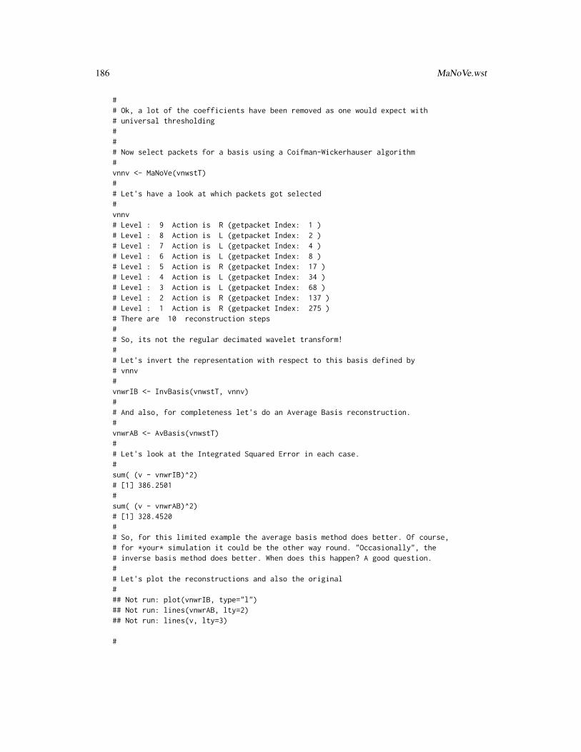
186 MaNoVe.wst

## Ok, a lot of the coefficients have been removed as one would expect with# universal thresholding### Now select packets for a basis using a Coifman-Wickerhauser algorithm#vnnv <- MaNoVe(vnwstT)## Let's have a look at which packets got selected#vnnv# Level : 9 Action is R (getpacket Index: 1 )# Level : 8 Action is L (getpacket Index: 2 )# Level : 7 Action is L (getpacket Index: 4 )# Level : 6 Action is L (getpacket Index: 8 )# Level : 5 Action is R (getpacket Index: 17 )# Level : 4 Action is L (getpacket Index: 34 )# Level : 3 Action is L (getpacket Index: 68 )# Level : 2 Action is R (getpacket Index: 137 )# Level : 1 Action is R (getpacket Index: 275 )# There are 10 reconstruction steps## So, its not the regular decimated wavelet transform!## Let's invert the representation with respect to this basis defined by# vnnv#vnwrIB <- InvBasis(vnwstT, vnnv)## And also, for completeness let's do an Average Basis reconstruction.#vnwrAB <- AvBasis(vnwstT)## Let's look at the Integrated Squared Error in each case.#sum( (v - vnwrIB)^2)# [1] 386.2501#sum( (v - vnwrAB)^2)# [1] 328.4520## So, for this limited example the average basis method does better. Of course,# for *your* simulation it could be the other way round. "Occasionally", the# inverse basis method does better. When does this happen? A good question.## Let's plot the reconstructions and also the original### Not run: plot(vnwrIB, type="l")## Not run: lines(vnwrAB, lty=2)## Not run: lines(v, lty=3)

#

mfilter.select 187

# The dotted line is the original. Neither reconstruction picks up the# spikes in heavisine very well. The average basis method does track the# original signal more closely though.#

mfilter.select Provide filter coefficients for multiple wavelets.

Description

This function returns the filter coefficients necessary for doing a discrete multiple wavelet transform(and its inverse).

Usage

mfilter.select(type = "Geronimo")

Arguments

type The name for the multiple wavelet basis. The two possible types are "Geronimo"and "Donovan3".

Details

This function supplies the multiple wavelet filter coefficients required by the mwd function.

A multiple wavelet filter is somewhat different from a single wavelet filter. Firstly the filters aremade up of matrices not single coefficients. Secondly there is no simple expression for the high passcoefficients G in terms of the low pass coefficients H, so both sets of coefficients must be specified.Note also that the transpose of the filter coefficients are used in the inverse transform, an unnecessarydetail with scalar coefficients. There are two filters available at the moment. Geronimo is thedefault, and is recommended as it has been checked thoroughly. Donovan3 uses three orthogonalwavelets described in Donovan et al. but this coding has had little testing.

See Donovan, Geronimo and Hardin, 1996 and Geronimo, Hardin and Massopust, 1994.

This function fulfils the same purpose as the filter.select function does for the standard DWTwd.

Value

A list is returned with the following eight components which describe the filter:

type The multiple wavelet basis type string.

H A vector containing the low pass filter coefficients.

G A vector containing the high pass pass filter coefficients.

name A character string containing the full name of the filter.

nphi The number of scaling functions in the multiple wavelet basis.

npsi The number of wavelet functions in the multiple wavelet basis.

188 mfilter.select

NH The number of matrix coefficients in the filter. This is different from length(H).

ndecim The decimation factor. I.e. the scale ratio between two successive resolutionlevels.

RELEASE

Version 3.9.6 (Although Copyright Tim Downie 1995-6)

Author(s)

Tim Downie

See Also

accessC.mwd, accessD.mwd, draw.mwd, mfirst.last, mwd.object, mwd, mwr, plot.mwd, print.mwd,putC.mwd, putD.mwd, summary.mwd, threshold.mwd, wd, wr.mwd.

Examples

#This function is currently used by `mwr' and `mwd' in decomposing and#reconstructing, however you can view the coefficients.## look at the filter coefficients for Geronimo multiwavelet#mfilter.select()#$type:#[1] "Geronimo"##$name:#[1] "Geronimo Multiwavelets"##$nphi:#[1] 2##$npsi:#[1] 2##$NH:#[1] 4##$ndecim:#[1] 2#$H:# [1] 0.4242641 0.8000000 -0.0500000 -0.2121320 0.4242641 0.0000000# [7] 0.4500000 0.7071068 0.0000000 0.0000000 0.4500000 -0.2121320#[13] 0.0000000 0.0000000 -0.0500000 0.0000000##$G:# [1] -0.05000000 -0.21213203 0.07071068 0.30000000 0.45000000 -0.70710678## [7] -0.63639610 0.00000000 0.45000000 -0.21213203 0.63639610 -0.30000000#[13] -0.05000000 0.00000000 -0.07071068 0.00000000

mfirst.last 189

mfirst.last Build a first/last database for multiple wavelet transforms.

Description

This function is not intended for user use, but is used by various functions involved in computingand displaying multiple wavelet transforms.

Usage

mfirst.last(LengthH, nlevels, ndecim, type = "wavelet", bc = "periodic")

Arguments

LengthH Number of filter matrix coefficients.

nlevels Number of levels in the decomposition

ndecim The decimation scale factor for the multiple wavelet basis.

type Whether the transform is non-decimated or ordinary (wavelet). The non-decimatedmultiple wavelet transform is not yet supported.

bc This argument determines how the boundaries of the the function are to be han-dled. The permitted values are periodic or symmetric

Details

Suppose you begin with 2^m=2048 coefficient vectors. At the next level you would expect 1024smoothed data vectors, and 1024 wavelet vectors, and if bc="periodic" this is indeed what hap-pens. However, if bc="symmetric" you actually need more than 1024 (as the wavelets extend overthe edges). The first last database keeps track of where all these "extras" appear and also where theyare located in the packed vectors C and D of pyramidal coefficients within wavelet structures.

For examples, given a first.last.c row of

−2320

The ‘position’ of the coefficient vectors would be

c−2, c−1, c0, c1, c2, c3

In other words, there are 6 coefficients, starting at -2 and ending at 3, and the first of these (c−2)appears at column 20 of the $C component matrix of the wavelet structure.

You can “do” first.last in your head for periodic boundary handling but for more general boundarytreatments (e.g. symmetric) first.last is indispensable.

The numbers in first last databases were worked out from inequalities derived from: Daubechies, I.(1988).

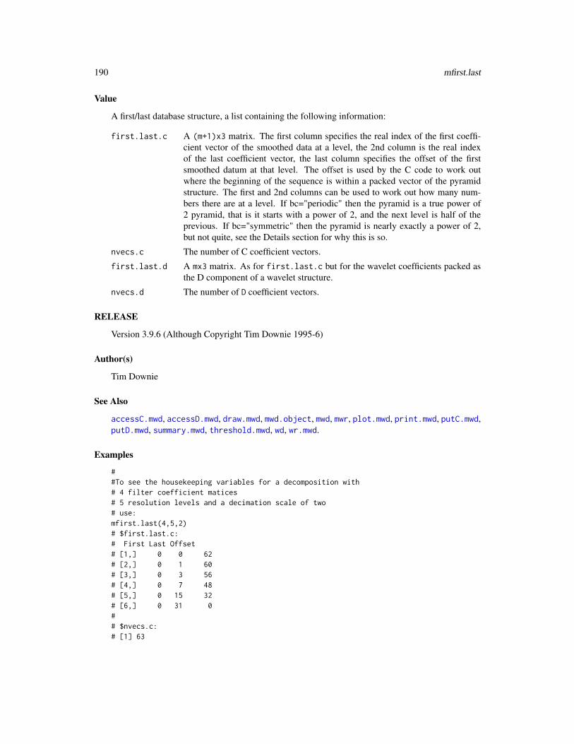
190 mfirst.last

Value

A first/last database structure, a list containing the following information:

first.last.c A (m+1)x3 matrix. The first column specifies the real index of the first coeffi-cient vector of the smoothed data at a level, the 2nd column is the real indexof the last coefficient vector, the last column specifies the offset of the firstsmoothed datum at that level. The offset is used by the C code to work outwhere the beginning of the sequence is within a packed vector of the pyramidstructure. The first and 2nd columns can be used to work out how many num-bers there are at a level. If bc="periodic" then the pyramid is a true power of2 pyramid, that is it starts with a power of 2, and the next level is half of theprevious. If bc="symmetric" then the pyramid is nearly exactly a power of 2,but not quite, see the Details section for why this is so.

nvecs.c The number of C coefficient vectors.

first.last.d A mx3 matrix. As for first.last.c but for the wavelet coefficients packed asthe D component of a wavelet structure.

nvecs.d The number of D coefficient vectors.

RELEASE


Author(s)

Tim Downie

See Also

accessC.mwd, accessD.mwd, draw.mwd, mwd.object, mwd, mwr, plot.mwd, print.mwd, putC.mwd,putD.mwd, summary.mwd, threshold.mwd, wd, wr.mwd.

Examples

##To see the housekeeping variables for a decomposition with# 4 filter coefficient matices# 5 resolution levels and a decimation scale of two# use:mfirst.last(4,5,2)# $first.last.c:# First Last Offset# [1,] 0 0 62# [2,] 0 1 60# [3,] 0 3 56# [4,] 0 7 48# [5,] 0 15 32# [6,] 0 31 0## $nvecs.c:# [1] 63

modernise 191

## $first.last.d:# First Last Offset# [1,] 0 0 30# [2,] 0 1 28# [3,] 0 3 24# [4,] 0 7 16# [5,] 0 15 0## $nvecs.d:# [1] 31

modernise Generic function to upgrade a V2 WaveThresh object to V4

Description

Not really used in practice. The function IsEarly can be used to tell if an object comes from anearlier version of wavethresh. Note that the earlier version only has a wd.object class object sothere is only a method for that.

Usage

modernise(...)

Arguments

... Other objects

Details


Value

A modernised version of the object.

Author(s)

G P Nason

See Also

IsEarly,modernise.wd

192 mpostfilter

modernise.wd Modernise a wd class object

Description

Upgrade a version 2 wd.object to version 4. The function IsEarly can tell if the object comesfrom an earlier version of WaveThresh.

Usage

## S3 method for class 'wd'modernise(wd, ...)

Arguments

wd The wd object you wish to modernise

... Other arguments

Details


Value

The modernised object.

Author(s)

G P Nason

mpostfilter Multiwavelet postfilter

Description

A multiwavelet postfilter turns a multivariate sequence into a univariate sequence. As such, thepostfilter is used on the inverse transform, it is the inverse of an earlier used prefilter.

Not intended for direct user use.

Usage

mpostfilter(C, prefilter.type, filter.type,nphi, npsi, ndecim, nlevels, verbose = FALSE)

mprefilter 193

Arguments

C The multivariate sequence you wish to turn back into a univariate one using theinverse of an earlier prefilter operation.

prefilter.type Controls the type of prefilter (see Tim Downie’s PhD thesis, or references therein.Types include Minimal, Identity, Repeat, Interp, default, Xia, Roach1,Roach3, Donovan3 or Linear

filter.type The type of multiwavelet: can be Geronimo or Donovan3

nphi The number of father wavelets in the system

npsi The number of mother wavelets in the system

ndecim The ndecim parameter (not apparently used here)

nlevels The number of levels in the multiwavelet transform

verbose If TRUE then informative messages are printed as the function progresses

Details


Value

The appropriate postfiltered data.

Author(s)

Tim Downie

See Also

mprefilter,mwd

mprefilter Multiwavelet prefilter

Description

A multiwavelet prefilter turns a univariate sequence into a bivariate (in this case) sequence suitablefor processing by a multiwavelet transform, such as mwd. As such, the prefilter is used on the forwardtransform.

Not intended for direct user use.

Usage

mprefilter(data, prefilter.type, filter.type, nlevels, nvecs.c,nphi, npsi, ndecim, verbose = FALSE)

194 mwd

Arguments

data The univariate sequence that you wish to turn into a multivariate one

prefilter.type Controls the type of prefilter (see Tim Downie’s PhD thesis, or references therein.Types include Minimal, Identity, Repeat, Interp, default, Xia, Roach1,Roach3, Donovan3 or Linear

filter.type The type of multiwavelet: can be Geronimo or Donovan3

nlevels The number of levels in the multiwavelet transform

nvecs.c Parameter obtained from the mfirst.last function related to the particular filters

nphi The number of father wavelets in the system

npsi The number of mother wavelets in the system

ndecim The ndecim parameter (not apparently used here)

verbose If TRUE then informative messages are printed as the function progresses

Details


Value

The appropriate prefiltered data.

Author(s)

Tim Downie

See Also

mpostfilter,mwd

mwd Discrete multiple wavelet transform (decomposition).

Description

This function performs the discrete multiple wavelet transform (DMWT). Using an adaption ofMallat’s pyramidal algorithm. The DMWT gives vector wavelet coefficients.

Usage

mwd(data, prefilter.type = "default", filter.type = "Geronimo",bc ="periodic", verbose = FALSE)

mwd 195

Arguments

data A vector containing the data you wish to decompose. The length of this vec-tor must be a power of 2 times the dimension of the DMWT (multiplicity ofwavelets).

prefilter.type This chooses the method of preprocessing required. The arguments will dependon filter.type, but "default" will always work.

filter.type Specifies which multi wavelet filter to use, The options are "Geronimo" (dimen-sion 2) or "Donovan3" (dimension 3). The latter has not been tested fully andmay contain bugs. See the function mfilter.select for further details.

bc specifies the boundary handling. If bc=="periodic" the default, then the func-tion you decompose is assumed to be periodic on its interval of definition, ifbc=="symmetric" then the function beyond its boundaries is assumed to be asymmetric reflection of the function in the boundary.


Details

The code implements Mallat’s pyramid algorithm adapted for multiple wavelets using Xia, Geron-imo, Hardin and Suter, 1996. The method takes a data vector of length 2^J*M, and preprocesses it.This has two effects, firstly it puts the data into matrix form and then filters it so that the DMWT canoperate more efficiently Most of the technical details are similar to the single wavelet transform ex-cept for the matrix algebra considerations, and the prefiltering process. See Downie and Silverman(1998) for further details and how this transform can be used in a statistical context.

Value

An object of class mwd.

RELEASE

Version 3.9.6 (Although Copyright Tim Downie 1996)

Author(s)

Tim Downie

See Also

accessC.mwd, accessD.mwd, draw.mwd, mfirst.last, mfilter.select, mwd.object, mwr, plot.mwd,print.mwd, putC.mwd, putD.mwd, summary.mwd, threshold.mwd, wd, wr.mwd.

Examples

## Generate some test data#test.data <- example.1()$y

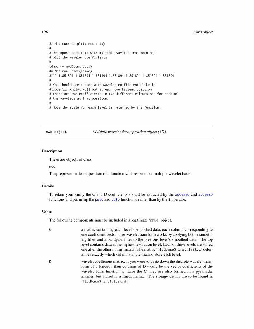
196 mwd.object

## Not run: ts.plot(test.data)## Decompose test.data with multiple wavelet transform and# plot the wavelet coefficients#tdmwd <- mwd(test.data)## Not run: plot(tdmwd)#[1] 1.851894 1.851894 1.851894 1.851894 1.851894 1.851894 1.851894## You should see a plot with wavelet coefficients like in#\code{\link{plot.wd}} but at each coefficient position# there are two coefficients in two different colours one for each of# the wavelets at that position.## Note the scale for each level is returned by the function.

mwd.object Multiple wavelet decomposition object (1D)

Description

These are objects of class

mwd

They represent a decomposition of a function with respect to a multiple wavelet basis.

Details

To retain your sanity the C and D coefficients should be extracted by the accessC and accessDfunctions and put using the putC and putD functions, rather than by the $ operator.

Value

The following components must be included in a legitimate ‘mwd’ object.

C a matrix containing each level’s smoothed data, each column corresponding toone coefficient vector. The wavelet transform works by applying both a smooth-ing filter and a bandpass filter to the previous level’s smoothed data. The toplevel contains data at the highest resolution level. Each of these levels are storedone after the other in this matrix. The matrix ‘fl.dbase$first.last.c’ deter-mines exactly which columns in the matrix, store each level.

D wavelet coefficient matrix. If you were to write down the discrete wavelet trans-form of a function then columns of D would be the vector coefficients of thewavelet basis function s. Like the C, they are also formed in a pyramidalmanner, but stored in a linear matrix. The storage details are to be found in‘fl.dbase$first.last.d’.

mwd.object 197

nlevelsWT The number of levels in the pyramidal decomposition that produces the coeffi-cients. The precise number of levels depends on the number of different waveletfunctions used and the preprocessing method used, as well as the number of datapoints used.

fl.dbase The first last database associated with this decomposition. This is a list con-sisting of 2 integers, and 2 matrices. The matrices detail how the coefficientsare stored in the C and D components of the ‘mwd.object’. See the help onmfirst.last for more information.

filter a list containing the details of the filter that did the decomposition. See mfilter.select.

type either "wavelet" indicating that the ordinary multiple wavelet transform wasperformed or "station" indicating that the non-decimated multiple wavelettransform was done.

prefilter Type of preprocessing or prefilter used. This will be specigic for the type ofmultiple wavelet used.

date The date that the transform was performed or the mwd object was last modified.

bc how the boundaries were handled

GENERATION

This class of objects is returned from the mwd function to represent a multiple wavelet decompositionof a function. Many other functions return an object of class mwd.

METHODS

The mwd class of objects has methods for the following generic functions: accessC, accessD,draw, plot, print, putC, putD, summary, threshold, wr.mwd.

RELEASE

Version 3.9.6 (Although Copyright Tim Downie, 1995-6).

Author(s)

Tim Downie

See Also

accessC.mwd, accessD.mwd, draw.mwd, mfirst.last, mfilter.select, mwd.object, mwr, plot.mwd,print.mwd,putC.mwd, putD.mwd, summary.mwd, threshold.mwd, wd, wr.mwd.

198 mwr

mwr Multiple discrete wavelet transform (reconstruction).

Description

This function performs the reconstruction stage of Mallat’s pyramid algorithm adapted for multiplewavelets (see Xia et al.(1996)), i.e. the discrete inverse multiple wavelet transform.

Usage

mwr(mwd, prefilter.type = mwd$prefilter, verbose = FALSE, start.level = 0,returnC = FALSE)

Arguments

mwd A multiple wavelet decomposition object as returned by mwd.

prefilter.type Usually best not to change this (i.e. not to use a different prefilter on the recon-struction to the one used on decomposition).


start.level The level you wish to start reconstruction at. The is usually the first (level 0).

returnC If this is FALSE then a vector of the same length as the argument data supplied tothe function mwd that constructed the supplied mwd.object. is returned, Ie. thereconstructed data. If true then the last level (highest resolution) C coefficientsare returned in matrix form. This matrix has not been postprocessed.

Details

The code implements Mallat’s pyramid algorithm adapted for multiple wavelet decompositions (Xiaet al. 1996). In the reconstruction the quadrature mirror filters G and H are supplied with C0 andD0, D1, ... D(J-1) (the wavelet coefficients) and rebuild C1,..., CJ.

The matrix CJ is postprocessed which returns the full reconstruction

If mwd.object was obtained directly from mwd then the original function can be reconstructuedexactly. Usually, the mwd.object has been modified in some way, for examples, some coefficientsset to zero by threshold. Mwr then reconstructs the function with that set of wavelet coefficients.

See also Downie and Silverman, 1998

Value

Either a vector containing the final reconstruction or a matrix containing unpostprocessed coeffi-cients.

RELEASE

Version 3.9.6 (Although Copyright Tim Downie 1996)

newsure 199

Author(s)

Tim Downie

See Also

accessC.mwd, accessD.mwd, draw.mwd, mfirst.last, mfilter.select, mwd, mwd.object, plot.mwd,print.mwd, putC.mwd, putD.mwd, summary.mwd, threshold.mwd, wd, wr.mwd.

Examples

## Decompose and then exactly reconstruct test.data#test.data <- rnorm(128)tdecomp <- mwd(test.data)trecons <- mwr(tdecomp)## Look at accuracy of reconstructionmax(abs(trecons - test.data))#[1] 2.266631e-12## See also the examples of using \code{\link{wr}} or mwr in# the \code{examples} section of# the help for \code{\link{threshold.mwd}}.

newsure Version of sure that acts as subsidiary for threshold.irregwd

Description

Version of the sure function used as a subsidiary for threshold.irregwd.

Usage

newsure(s, x)

Arguments

s Vector of standard deviations of coefficients

x Vector of regular (ie non-normalized) coefficients

Details


Value

The SURE threshold

200 nlevelsWT

Author(s)

Arne Kovac

See Also

sure, threshold.irregwd

nlevelsWT Returns number of scale (resolution) levels.

Description

Returns the number of scales (or resolutions) in various wavelet objects and for some objects returnsthe number of scales that would result if processed by a wavelet routine.


One methods exists at present as most wavelet objects store the number of levels as the nlevelsWTcomponent. The method that exists isnlevelsWT.default

Usage

nlevelsWT(...)

Arguments


Details


Value

An integer representing the number of levels associated with the object.

RELEASE


Author(s)

G P Nason

See Also

nlevelsWT.default

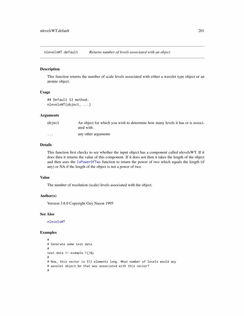
nlevelsWT.default 201

nlevelsWT.default Returns number of levels associated with an object

Description

This function returns the number of scale levels associated with either a wavelet type object or anatomic object.

Usage

## Default S3 method:nlevelsWT(object, ...)

Arguments

object An object for which you wish to determine how many levels it has or is associ-ated with.


Details

This function first checks to see whether the input object has a component called nlevelsWT. If itdoes then it returns the value of this component. If it does not then it takes the length of the objectand then uses the IsPowerOfTwo function to return the power of two which equals the length (ifany) or NA if the length of the object is not a power of two.

Value

The number of resolution (scale) levels associated with the object.

Author(s)


See Also

nlevelsWT

Examples

## Generate some test data#test.data <- example.1()$y## Now, this vector is 512 elements long. What number of levels would any# wavelet object be that was associated with this vector?#

202 nullevels

nlevelsWT(test.data)# [1] 9## I.e. 2^9=512. Let's check by taking the wavelet transform of the# test data and seeing how many levels it actually has#nlevelsWT(wd(test.data))# [1] 9

nullevels Set whole resolution levels of coefficients equal to zero.

Description

Generic function which sets whole resolution levels of coefficients equal to zero.


imwd use the nullevels.imwd method.

wd use the nullevels.wd method.

wst use the nullevels.wst method.


Usage

nullevels(...)

Arguments


Value

An object of the same class as x but with the specified levels set to zero.

RELEASE


Author(s)

G P Nason

See Also

nullevels.imwd nullevels.wd nullevels.wst wd.object, wd wst.object wst

nullevels.imwd 203

nullevels.imwd Sets whole resolution levels of coefficients equal to zero in a imwdobject.

Description

Sets whole resolution levels of coefficients equal to zero in a imwd.object

Usage

## S3 method for class 'imwd'nullevels(imwd, levelstonull, ...)

Arguments

imwd An object of class imwd.

levelstonull An integer vector specifying which resolution levels of coefficients of imwd thatyou wish to set to zero.


Details

Setting whole resolution levels of coefficients to zero can be very useful. For examples, one canconstruct a linear smoothing method by setting all coefficients above a particular resolution (theprimary resolution equal to zero. Also setting particular levels equal to zero can also be useful forremoving noise which is specific to a particular resolution level (as long as important signal is notalso contained at that level).

Note that this function removes the horiztonal, diagonal and vertical detail coefficients at the reso-lution level specified. It does not remove the father wavelet coefficients at those resolution levels.

To remove individual coefficients on a systematic basis you probably want to look at the thresholdfunction.

Value

An object of class imwd where the coefficients in resolution levels specified by levelstonull havebeen set to zero.

RELEASE


Author(s)

G P Nason

204 nullevels.wd

See Also

nullevels, imwd, imwd.object, threshold.

Examples

## Do the wavelet transform of the Lennon image#data(lennon)lenimwd <- imwd(lennon)## Set scales (resolution levels) 2, 4 and 6 equal to zero.#lenwdNL <- nullevels(lenimwd, levelstonull=c(2,4,6))## Now let's plot the coefficients using a nice blue-heat colour map## You will see that coefficients at levels 2, 4 and 6 are black (i.e. zero)# You can see that coefficients at other levels are unaffected and still# show the Lennon coefficients.### Not run: plot(lenwdNL)

nullevels.wd Sets whole resolution levels of coefficients equal to zero in a wd object.

Description

Sets whole resolution levels of coefficients equal to zero in a wd.object

Usage

## S3 method for class 'wd'nullevels(wd, levelstonull, ...)

Arguments

wd An object of class wd.

levelstonull An integer vector specifying which resolution levels of coefficients of wd thatyou wish to set to zero.


nullevels.wd 205

Details


Note that this function removes the horiztonal, diagonal and vertical detail coefficients at the reso-lution level specified. It does not remove the father wavelet coefficients at those resolution levels.


Value

An object of class wd where the coefficients in resolution levels specified by levelstonull havebeen set to zero.

RELEASE


Author(s)

G P Nason

See Also

nullevels, wd, wd.object, threshold.

Examples

## Generate some test data#test.data <- example.1()$y## Do wavelet transform of test.data and plot the wavelet coefficients#wds <- wd(test.data)## Not run: plot(wds)## Now let us set all the coefficients in ODD resolution levels equal to zero!## This is just to illustrate the capabilities of the function. I cannot# imagine you wanting to do this in practice!##wdsnl <- nullevels(wds, levelstonull = c(1, 3, 5, 7))## Now let's plot the result### Not run: plot(wdsnl, scaling = "by.level")

206 nullevels.wst

## Lo and behold the odd levels have been set to zero!

nullevels.wst Sets whole resolution levels of coefficients equal to zero in a wst object.

Description

Sets whole resolution levels of coefficients equal to zero in a wd object.

Usage

## S3 method for class 'wst'nullevels(wst, levelstonull, ...)

Arguments

wst An object of class wst.

levelstonull An integer vector specifying which resolution levels of coefficients of wst thatyou wish to set to zero.


Details



Value

An object of class wst where the coefficients in resolution levels specified by levelstonull havebeen set to zero.

RELEASE


Author(s)

G P Nason

See Also

nullevels, wst, wst.object, threshold.

numtonv 207

Examples

## Look at the examples for \code{\link{nullevels.wd}}.# The operation is almost identical except that \code{\link{wst}}# objects are replaced by \code{\link{wd}} ones.

numtonv Convert an index number into a node vector object.

Description

Convert an index number into a node vector object.

Usage

numtonv(number, nlevels)

Arguments

number The index number of a particular basis within a wavelet object.

nlevels The number of levels that the wavelet object has (can often be discovered usingthe nlevels function).

Details

A basis within a (e.g. non-decimated) wavelet object (such as a wst.object) is represented inWaveThresh by a nv or node vector.

A packet-ordered non-decimated wavelet transform object wst for short) which is the transform ofa vector of length n contains n bases. Each basis can be indexed from 0 to (n-1) .

A wst.object is simply a fully populated binary tree. There are nlevels levels in the tree with a splitat each level. The root of the tree is at level 0, there are two branches at level 1, four at level 2, eightat level 3 and so on. A path through the tree can be constructed by starting at the root and choosing"left" or "right" at each possible branch. For certain data situations this path is constructed usingminimum entropy algorithms (for examples MaNoVe). This function (numtonv takes the numericalrepresentation of a path and converts it into a node.vector form suitable for passing to InvBasisto invert the representation according to a basis specicified by number.

The least significant digit in number corresponds to deciding on the left/right decision at the fineleaves of the tree (high-frequency structure) and the most significant digit in number correspondsto deciding on the left/right decision at the root. Therefore gradually incrementing number from0 to 2^{nlevels}-1 steps through all possible bases in the wst object ranging from all decisionsbeing made "left" to all decisions being made "right". The "number" dividied by 2^{nlevels}corresponds exactly to the binary number epsilon in Nason and Silverman (1995).

Value

An object of class nv (node vector). This contains information about a path through a wavelet object(a basis in a wavelet object).

208 numtonv

RELEASE


Author(s)

G P Nason

See Also

wst, wst.object, MaNoVe, nv.object, InvBasis, nlevels.

Examples

## Generate some test data#test.data <- example.1()$y## Make it noisy#ynoise <- test.data + rnorm(512, sd=0.1)## Do packet ordered non-decimated wavelet transform#ynwst <- wst(ynoise)## Now threshold the coefficients#ynwstT <- threshold(ynwst)## Select basis number 9 (why not?)#NodeVector9 <- numtonv(9, nlevelsWT(ynwstT))## Let's print it out to see what it looks like# (nb, if you're repeating this examples, the basis might be different# as you may have generated different pseudo random noise to me)#NodeVector9# Level : 8 Action is R (getpacket Index: 1 )# Level : 7 Action is L (getpacket Index: 2 )# Level : 6 Action is L (getpacket Index: 4 )# Level : 5 Action is R (getpacket Index: 9 )# Level : 4 Action is L (getpacket Index: 18 )# Level : 3 Action is L (getpacket Index: 36 )# Level : 2 Action is L (getpacket Index: 72 )# Level : 1 Action is L (getpacket Index: 144 )# Level : 0 Action is L (getpacket Index: 288 )# There are 9 reconstruction steps## The print-out describes the tree through ynwstT that corresponds to# basis 9.

nv.object 209

## The NodeVector9 and ynwstT objects could now be supplied to# InvBasis.wst for inverting ynwstT according# to the NodeVector9 or basis number 9.

nv.object Node vector objects.

Description


nv

They represent a basis in a packet-ordered non-decimated wavelet transform object.

Details

A nv object is a description of a basis which is a path through a packet ordered non-decimatedwavelet transform. To view the basis just print it! See the examples in numtonv for a print out of itsstructure.

A similar object exists for describing a basis in a wavelet packet object see nvwp.

Value

The following components must be included in a legitimate ‘nv’ object.

node.list This is a complicated structure composed of one-dimensional array of nv$nlevelsWTlists. Each item in the array is itself a list having two components$upperctrland upperl. Each component is described as follows:upperctrl The ‘upperctrl’ item in each is the most important. It consists of a

vector of characters. Each character refers to a node in the non-decimatedwavelet tree at that level and can only be one of the characters L (for left),R (for right) and S (for stop). Each character in the vector informs recon-struction algorithms that, to do the best thing (whatever the best thing is inany particular case, e.g. select the minimum entropy node downwards), youshould select the left/right node or stop at the current node.

upperl The ‘upperl’ vector is in 1-1 correspondance with the ‘upperctrl’ vector.Each entry is a number related in some way to the L/R/S entry. (For theminumum entropy this is the minmum entropy achieved by this selection).

nlevelsWT The number of levels in the wst object that was involved in thecreation of the nv object. Nv objects describe a basis relative to a packetordered non-decimated wavelet transform object and thus must know thenumber of levels in that object.

GENERATION

This class of objects is returned from the MaNoVe.wst and numtonv functions. The former returnsthe minimum entropy basis (most sparse basis) obtained using the Coifman-Wickerhauser, 1992algorithm. The latter permits selection of a basis by an index number.

210 plot.imwd

METHODS

The nv class of objects has methods for the following generic functions: print, nlevelsWT, InvBasis,

RELEASE


Author(s)

G P Nason

See Also

wst, wst.object, numtonv, print, nlevelsWT, InvBasis, MaNoVe.wst.

plot.imwd Draw a picture of the 2D wavelet coefficients using image

Description

This function images 2D the absolute values discrete wavelet transform coefficients arising from aimwd.object object.

Usage

## S3 method for class 'imwd'plot(x, scaling = "by.level", co.type = "abs",package = "R", plot.type = "mallat", arrangement = c(3, 3),transform = FALSE, tfunction = sqrt, ...)## S3 method for class 'imwdc'plot(x, verbose=FALSE, ...)

Arguments

x The 2D imwd object you wish to depict

scaling How coefficient scaling is performed. The options are by.level to scale thecoefficients independently by level, anything else causes coefficients to be scaledglobally

co.type Can be "abs" for the absolute values of the coefficients to be plotted, can be"mabs" for the negative absolute values or "none" for none of this.

package Can be "R" for the R package, or "S". The latter does less interesting things andresults in a simpler plot

plot.type If this argument is "mallat" the coefficients at different scales and orientationsare packed into one image and plotted, a format originating from Mallat’s earlypapers on this. The other possibility is "cols" which plots each combination ofscale and direction on a separate plot. This latter format is useful for examiningcoefficients, especially at the coarser scales.

plot.irregwd 211

arrangement If plot.type="cols" then this argument specifies how many rows and columnsthere are in the plot array.

transform If FALSE then the coefficients are plotted as they are (subject to the co.typeargument above), if TRUE then the transform function supplied by tfunctionis applied to the coefficients.

tfunction If transform=TRUE then this function gets applied to transform the coefficientsbefore plotting

verbose Print out informative messages

... Supply other arguments to the call to the image function. This is very useful to,e.g., can the colours, or other aspects of the image

Details


Value

If the package="S" argument is set then a matrix is returned containing the image that would havebeen plotted (and this only works if the plot.type="mallat" argument is set also.

Author(s)

G P Nason

See Also

imwd, imwd.object, threshold.imwd

Examples

data(lennon)lwd <- imwd(lennon)## Not run: plot(lwd)## Not run: plot(lwd, col=grey(seq(from=0, to=1, length=100)), transform=TRUE)

plot.irregwd Plot variance factors of wavelet transform coefficients for irregularlyspaced wavelet transform object

Description

This function plots the variance factors associated with the wavelet coefficients arising from airregwd.objects irregularly spaced wavelet decomposition object.

212 plot.irregwd

Usage

## S3 method for class 'irregwd'plot(x, xlabels, first.level = 1,main = "Wavelet Decomposition Coefficients", scaling = "by.level",rhlab = FALSE, sub, ...)

Arguments

x The irregwd.objects object whose coefficients you wish to plot.

xlabels A vector containing the "true" x-axis numbers that went with the vector that wastransformed to produce the irregwd object supplied as the first argument to thisfunction. If this argument is missing then the function tries to make up a sensibleset of x-axis labels.

first.level The first resolution level to begin plotting at. This argument can be quite usefulwhen you want to supress some of the coarser levels in the diagram.

main The main title of the plot.

scaling How you want the coefficients to be scaled. The options are: global - one scalefactor is chosen for the whole plot. The scale factor depends on the variancefactor to be included on the plot that has the largest absolute value. The globaloption is useful when comparing factors that might appear anywhere in the plot;by.level - a scale factor is chosen for each resolution level in the plot. Thescale factor for a level depends on the variance factor in that level that has thelargest absolute value. The by.level option is useful when you wish to comparecoefficients within a resolution level.

rhlab If TRUE then a set of labels is produced on the right hand axis. The axis la-bels in this case refer to the scale factors used to scale each level and corre-spond to value of the largest variance factor (in absolute value) in each scale(when scaling=="by.level") or absolutely (when scaling="global"). If therhlab=FALSE then no right hand axis labels are produced.

sub A subtitle for the plot.

... Other arguments supplied to the actual plot

Details

Produces a plot similar in style to the ones in Donoho and Johnstone, 1994. This function is basi-cally the same as plot.wd except that variance factors and not coefficients are plotted. A variancefactor is a number that quantifies the variability of a coefficient induced by the irregular design thatwas interpolated to a regular grid by the makegrid function which is used the by irregwd irregularwavelet transform function.

High values of the variance factor correspond to large variance in the wavelet coefficients but dueto the irregular design, not the original noise structure on the coefficients.

Value

If rhlab==TRUE then the scaling factors applied to each scale level are returned. Otherwise NULL isreturned.

plot.mwd 213

Author(s)

Arne Kovac

Examples

## The help for makegrid contains an example# of using this function.#

plot.mwd Use plot on an mwd object.

Description

Plots the wavelet coefficients of a mwd class object.

Usage

## S3 method for class 'mwd'plot(x, first.level = 1, main = "Wavelet Decomposition Coefficients",

scaling = "compensated", rhlab = FALSE, sub = x$filter$name,NotPlotVal = 0.05, xlab = "Translate", ylab = "Resolution level",return.scale = TRUE, colour = (2:(npsi + 1)), ...)

Arguments

x The mwd object whose coefficients you wish to plot.first.level The first resolution level to begin plotting at. This argument can be quite useful

when you want to supress some of the coarser levels in the diagram.main The main title of the plot.scaling How you want the coefficients to be scaled. The options are: "global" - one

scale factor is chosen for the whole plot. The scale factor depends on the coef-ficient to be included on the plot that has the largest absolute value. The globaloption is useful when comparing coefficients that might appear anywhere in theplot; "by.level" - a scale factor is chosen for each resolution level in the plot.The scale factor for a level depends on the coefficient in that level that has thelargest absolute value. The "by.level" option is useful when you wish to com-pare coefficients within a resolution level.The other option is "compensated" which is the same as "global" except forthat finer scales’ coefficients are scaled up by a factor of SQRT(2) for compensated.This latter options is sometimes useful.

rhlab If T then a set of labels is produced on the right hand axis. The axis labels in thiscase refer to the scale factors used to scale each level and correspond to value ofthe largest coefficient (in absolute value) in each scale (when scaling=="by.level")or absolutely (when scaling="global"). If the rhlab argument is FALSE thenno right hand axis labels are produced.

214 plot.mwd


NotPlotVal Doesn’t seem to be implemented.

xlab A title for the x-axis

ylab A title for the y-axis

return.scale If true (default) the scale for each resolution level is returned

colour A vector of length mwd$npsi, the values of which are the colours used to plotthe coefficients, one for each distinct type of wavelet (with apologies to ourAmerican cousins for spelling colour correctly!)

... other arguments to be supplied to plot.

Details

Produces a plot similar to the ones in Donoho and Johnstone, 1994.

Wavelet coefficients for each resolution level are plotted one above the other, with the high res-olution coefficients at the bottom, and the low resolution at the top. Each vector is representedby mwd$npsi lines one for each element in the coefficient vector. If colour is supported by thedevice each element will be represented by a different coulour. The coefficients are plotted usingthe segment function, with a large positive coefficient being plotted above an imaginary horizontalcentre line, and a large negative coefficient plotted below it. The position of a coefficient along aline is indicative of the wavelet basis function’s translate number.

The resolution levels are labelled on the left-hand side axis, and the maximum values of the absolutevalues of the coefficients for the particular level form the right-hand side axis.

The levels of coefficients can be scaled in three ways. If you are not interested in comparing therelative scales of coefficients from different levels, then the default scaling option, "by.level" iswhat you need. This computes the maximum of the absolute value of the coefficients at a particularlevel and scales the so that the fit nicely onto the plot. For this option, each level is scaled DIFFER-ENTLY. To obtain a uniform scale for all the levels specify the "global" option to the scalingargument. This will allow you to make inter-level comparisons.

Value

Axis labels for each resolution level unless return.scale=F when NULL is returned. The axisvalues are the maximum of the absolute value of the coefficients at that resolution level. They arereturned because they are sometimes hard to read on the plot.

RELEASE


Note

A plot of the coefficients contained within the mwd object at each resolution level is produced.

Author(s)

G P Nason

plot.nvwp 215

See Also

accessC.mwd, accessD.mwd, draw.mwd, mfirst.last, mfilter.select, mwd, mwd.object, mwr,print.mwd, putC.mwd, putD.mwd, summary.mwd, threshold.mwd, wd, wr.mwd.

Examples

## Generate some test data#test.data <- example.1()$y## Not run: ts.plot(test.data)## Decompose test.data with multiple wavelet transform and# plot the wavelet coefficients#tdmwd <- mwd(test.data)## Not run: plot(tdmwd)#[1] 1.851894 1.851894 1.851894 1.851894 1.851894 1.851894 1.851894## You should see a plot with wavelet coefficients like in# plot.wd but at each coefficient position# there are two coefficients in two different colours one for each of# the wavelets at that position.## Note the scale for each level is returned by the function.

plot.nvwp Depict wavelet packet basis specfication

Description

The nvwp class object (generated from MaNoVe.wp for example) contains a wavelet packet basisspecification. This function produces a graphical depiction of such a basis.

Usage

## S3 method for class 'nvwp'plot(x, ...)

Arguments

x The wavelet packet node vector you wish to plot, nvwp class object

... Other arguments to the central plot function

Details

The vertical axis indicates the resolution level, the horizontal axes indicates the packet index for thefinest scales.

216 plot.wd

Value

Nothing

Author(s)

G P Nason

See Also

MaNoVe.wp,print.nvwp,wp

Examples

v <- rnorm(512)vwp <- wp(v)vnv <- MaNoVe(vwp)## Not run: plot(vnv)

plot.wd Plot wavelet transform coefficients.

Description

This function plots discrete wavelet transform coefficients arising from a wd object.

Usage

## S3 method for class 'wd'plot(x,xlabvals, xlabchars, ylabchars, first.level = 0,main = "Wavelet Decomposition Coefficients", scaling = "global",rhlab = FALSE, sub, NotPlotVal = 0.005, xlab = "Translate",ylab = "Resolution Level",aspect = "Identity", ...)

Arguments

x The wd class object you wish to plot

xlabvals A vector containing the "true" x-axis numbers that went with the vector thatwas transformed to produce the wd object supplied as the first argument to thisfunction. If this argument is missing then the function tries to make up a sensibleset of x-axis labels.

xlabchars Tickmark labels for the x axis

ylabchars Tickmark labels for the y axis



plot.wd 217

scaling How you want the coefficients to be scaled. The options are: global - one scalefactor is chosen for the whole plot. The scale factor depends on the coefficientto be included on the plot that has the largest absolute value. The global optionis useful when comparing coefficients that might appear anywhere in the plot;by.level - a scale factor is chosen for each resolution level in the plot. Thescale factor for a level depends on the coefficient in that level that has the largestabsolute value. The by.level option is useful when you wish to compare coef-ficients within a resolution level.The two other options are compensated and super which are the same as globalexcept for that finer scales’ coefficients are scaled up by a factor of SQRT(2)for compensated and 2 for super. These latter two options are sometimes useful(more useful for non-decimated wd objects, where they act as a sort of ipndacwmatrix operator).

rhlab If TRUE then a set of labels is produced on the right hand axis. The axis la-bels in this case refer to the scale factors used to scale each level and corre-spond to value of the largest coefficient (in absolute value) in each scale (whenscaling=="by.level") or absolutely (when scaling="global"). If the rhlabargument is FALSE then no right hand axis labels are produced.


NotPlotVal This argument ensures that if all (scaled) coefficients in a resolution level arebelow NotPlotVal in absolute value then the whole resolution level is not plot-ted. This can be useful when plotting a wd object that is sparse (or has beenthresholded and necessarily many coefficients might well be zero) as it speedsup the plot because whole levels do not have to be plotted (the function thatdoes the plotting [segments()] is quite a slow function). Note that the value ofNotPlotVal refers to scaled coefficients, those that have been scaled by thisfunction (on any resolution level all coefficients are scaled to lie between -0.5and 0.5).

xlab A title for the x-axis

ylab A title for the y-axis

aspect This argument describes the name (as a character string) of a function to be ap-plied to the coefficients before plotting. By default the argument is "Identity",i.e. the coefficients are plotted as is. This argument is most useful when acomplex-valued wavelets are plotted you could use "Mod" to plot the modulusof the coefficients, or "Re" to plot the real parts of the coefficients or "Arg" toplot the argument of the coefficients. Also, the aspect argument can be usefulfor the ordinary wavelet transforms as well if you are interested in a particulartransform of the coefficients.

... fine tuning

Details

Produces a plot similar to the ones in Donoho and Johnstone, 1994.

A wavelet decomposition of a signal consists of discrete wavelet coefficients at different scales(resolution levels) and locations. This function plots the coefficients as a pyramid (derived fromMallat’s pyramid algorithm). See the examples below.

218 plot.wd

The resolution levels are stacked one above the other: coarse scale coefficients are always towardsthe top of the plot, fine scale coefficients are always located toward the bottom of the plot. Thelocation of coefficients increases from left to right across the plot in synchrony with the input signalto the wd object. In other words the position of a coefficient along a line is indicative of the asso-ciated wavelet basis function’s translate number. The actual coefficients are plotted using S-Plus’ssegments() function. This plots each coefficient as a vertical line with positive coefficients beingplotted above an imaginary centre line and negative coefficients being plotted below.

The resolution levels are labelled on the left-hand side axis, and if rhlab==T the maximum valuesof the absolute values of the coefficients, for the particular level, are plotted on the right-hand axis.

The coefficients in the plot may be scaled in 4 ways. If you are interested in comparing coefficientsin different levels then the default scaling option scaling=="global" is what you need. Thisworks by finding the coefficient with the largest absolute value amongst all coeffients to be plottedand then scales all the other coefficients by the largest so that all coefficients lie in the range -1/2to 1/2. The scaled coefficients are then plotted. If you are not interested in comparing relativeresolution levels and want to see all that goes on within a particular scale then you should use thescaling option scaling=="by.level" which picks out the largest coefficient (in absolute value)from each level and scales each level separately. The "compensated" and super options are like the"global" option except that finer levels are scaled up (as discussed in the arguments list above):this can be useful when plotting non-decimated wavelet transform coefficients as it emphasizes thehigher frequencies.

Value

If rhlab==T then the scaling factors applied to each scale level are returned. Otherwise NULL isreturned.

RELEASE


Note

A plot of the coefficients contained within the wd object is produced.

Author(s)

G P Nason

See Also

wd

Examples

## Generate some test data#test.data <- example.1()$y## Not run: ts.plot(test.data)#

plot.wp 219

# Decompose test.data and plot the wavelet coefficients#wds <- wd(test.data)## Not run: plot(wds)## Now do the time-ordered non-decimated wavelet transform of the same thing### Not run: wdS <- wd(test.data, type="station")## Not run: plot(wdS)## Next examples# ------------# The chirp signal is also another good examples to use.## Generate some test data#test.chirp <- simchirp()$y## Not run: ts.plot(test.chirp, main="Simulated chirp signal")## Now let's do the time-ordered non-decimated wavelet transform.# For a change let's use Daubechies least-asymmetric phase wavelet with 8# vanishing moments (a totally arbitrary choice, please don't read# anything into it).#chirpwdS <- wd(test.chirp, filter.number=8, family="DaubLeAsymm", type="station")## Not run: plot(chirpwdS, main="TOND WT of Chirp signal")

plot.wp Plot wavelet packet transform coefficients

Description

This function plots wavelet packet transform coefficients arising from a wp.object object.

Usage

## S3 method for class 'wp'plot(x, nvwp = NULL, main = "Wavelet Packet Decomposition",

sub, first.level = 5, scaling = "compensated", dotted.turn.on = 5,color.force = FALSE, WaveletColor = 2, NodeVecColor = 3,fast = FALSE, SmoothedLines = TRUE, ...)

Arguments

x The wp object whose coefficients you wish to plot.

nvwp An optional associated wavelet packet node vector class object of class nvwp.This object is a list of packets in the wavelet packet table. If this argument isspecified then it is possible to highlight the packets in the nvwp objects in adifferent color using the NodeVecColor argument

220 plot.wp




scaling How you want the coefficients to be scaled. The options are: global - one scalefactor is chosen for the whole plot. The scale factor depends on the coefficientto be included on the plot that has the largest absolute value. The global optionis useful when comparing coefficients that might appear anywhere in the plot;by.level - a scale factor is chosen for each resolution level in the plot. Thescale factor for a level depends on the coefficient in that level that has the largestabsolute value. The by.level option is useful when you wish to compare coef-ficients within a resolution level. The other option is compensated which is thesame as global except for that finer scales’ coefficients are scaled up by a factorof SQRT(2)I don’t know why compensated is the default option? That is probably silly!

dotted.turn.on The plot usually includes some dotted vertical bars that separate wavelet packetsto make it clearer which packets are which. This option controls the coarsestresolution level at which dotted lines appear. All levels equal to and finer thanthis level will receive the vertical dotted lines.

color.force If FALSE then some "clever" code in CanUseMoreThanOneColor tries to figureout how many colours can be used (THIS HAS NOT BEEN MADE TO WORKIN R) and hence whether colour can be used to pick out wavelet packets orelements of a node vector. This option was designed to work with S. It doesn’twork with R and so it is probably best to set color.force=T. In this way nointerrogation is done and the lines/packets are plotted in the appropriate colourswith no questions asked.

WaveletColor A colour specification for the colour for wavelet coefficients. Wavelet coef-ficients are a component of wavelet packet coefficients and this option allowsthem to be drawn in a different color. In R you can use names like "red", "blue"to select the colors. In R you’ll also need to set the color.force option to TRUE.

NodeVecColor If a nvwp object is supplied this option can force coefficients that are partof that nvwp to be drawn in the specified color. See the explanation for theWaveletColor option above about specification in R.

fast This option no longer does anything.

SmoothedLines If TRUE then the scaling function coefficients are drawn using lines (and looklike mini versions of the original). If FALSE then the scaling function coeffi-cients are drawn using the segments function and look like a coarser shadowyversion of the original.

... Other arguments to the plot command

Details

A wavelet packet object contains wavelet packet coefficients of a signal (usually obtained by the wpwavelet packet transform function). Given a wavelet packet object wp it possesses nlevelsWT(wp)resolution levels. In WaveThresh the coarsest level is level 0 and the finest is level nlevelsWT-1.For wavelet packets the number of packets at level j is 2^(nlevelsWT-j).

plot.wp 221

This function plots the wavelet packet coefficients. At the bottom of the plot the original inputfunction (if present) is plotted. Then levels above the original plot successively coarser waveletpacket coefficients. From the Mallat transform point of view smoothing goes up off the the left ofthe picture and detail to the right. The packets are indexed from 0 to the number of packets goingfrom left to right within each resolution level.

The function has the ability to draw wavelet coefficients in a different color using the WaveletColorargument.

Optionally, if a node vector wavelet packet object is also supplied, which contains the specificationof a basis selected from the packet table, then packets in that node vector can be highlighted in aanother colour determined by the NodeVecColor.

Packets are drawn on the plot and can be separated by vertical dotted lines. The resolution levels atwhich this happens can be controlled by the dotted.turn.on option. The coarsest resolution levelto be drawn is controlled by the first.level option.

Value

Nothing

Author(s)

G P Nason

See Also

MaNoVe, wp, wp.object

Examples

## Generate some test data#v <- DJ.EX()$blocks## Let's plot these to see what they look like### Not run: plot(v, type="l")## Do a wavelet packet transform#vwp <- wp(v)## And create a node vector#vnv <- MaNoVe(vwp)## Now plot the wavelet packets with the associated node vector### Not run: plot(vwp, vnv, color.force=T, WaveletColor="red", dotted.turn.on=7)## The wavelet coefficients are plotted in red. Packets from the node vector

222 plot.wst

# are depicted in green. The node vector gets plotted after the wavelet# coefficients so the green packets overlay the red (retry the plot command# but without the vnv object to see just the# wavelet coefficients). The vertical dotted lines start at resolution# level 7.##

plot.wst Plot packet-ordered non-decimated wavelet transform coefficients.

Description

This function plots packet-ordered non-decimated wavelet transform coefficients arising from awst.object object.

Usage

## S3 method for class 'wst'plot(x, main = "Nondecimated Wavelet (Packet) Decomposition",

sub, first.level = 5, scaling = "compensated", dotted.turn.on = 5,aspect = "Identity", ...)

Arguments

x The wst object whose coefficients you wish to plot.



first.level The first resolution level to begin plotting at. This argument can be quite usefulwhen you want to suppress some of the coarser levels in the diagram.

scaling How you want the coefficients to be scaled. The options are: global - one scalefactor is chosen for the whole plot. The scale factor depends on the coefficientto be included on the plot that has the largest absolute value. The global optionis useful when comparing coefficients that might appear anywhere in the plot;by.level - a scale factor is chosen for each resolution level in the plot. Thescale factor for a level depends on the coefficient in that level that has the largestabsolute value. The by.level option is useful when you wish to compare coef-ficients within a resolution level. The other option is compensated which is thesame as global except for that finer scales’ coefficients are scaled up by a factorof SQRT(2)I don’t know why compensated is the default option? It is a bit silly.

dotted.turn.on The plot usually includes some dotted vertical bars that separate wavelet packetsto make it clearer which packets are which. This option controls the coarsestresolution level at which dotted lines appear. All levels equal to and finer thanthis level will receive the vertical dotted lines.

plot.wst 223

aspect A transform to apply to the coefficients before plotting. If the coefficients arecomplex-valued and aspect="Identity" then the modulus of the coefficients areplotted.

... Other arguments to plot

Details

A packet-ordered non-decimated wavelet object contains coefficients of a signal (usually obtainedby the wst packet-ordered non-decimated wavelet transform, but also functions that derive suchobjects, such as threshold.wst).

A packet-ordered nondecimated wavelet object, x, possesses nlevelsWT(x) resolution levels. InWaveThresh the coarsest level is level 0 and the finest is level nlevelsWT-1. For packet-orderednondecimated wavelet the number of blocks (packets) at level j is 2^(nlevelsWT-j).

This function plots the coefficients. At the bottom of the plot the original input function (if present)is plotted. Then levels above the original plot successively coarser wavelet coefficients. Each packetof coefficients is plotted within dotted vertical lines. At the finest level there are two packets: one(the left one) correspond to the wavelet coefficients that would be obtained using the (standard)decimated wavelet transform function, wd, and the other packet are those coefficients that wouldhave been obtained using the standard decimated wavelet transform after a unit cyclic shift.

For coarser levels there are more packets corresponding to different cyclic shifts (although thecomputation is not performed using shifting operations the effect is the same). For full details seeNason and Silverman, 1995.

Packets are drawn on the plot and can be separated by vertical dotted lines. The resolution levels atwhich this happens can be controlled by the dotted.turn.on option. The coarsest resolution levelto be drawn is controlled by the first.level option.

It should be noted that the packets referred to here are just the blocks of nondecimated waveletcoefficients in a packet-ordering. These are different to wavelet packets (produced by wp) andnondecimated wavelet packets (produced by wpst)

Value

Nothing

Author(s)

G P Nason

See Also

MaNoVe,threshold.wst, wst, wst.object

Examples

## Generate some test data#v <- DJ.EX()$heavi#

224 plot.wst2D

# Let's plot these to see what they look like### Not run: plot(v, type="l")## Do a packet-ordered non-decimated wavelet packet transform#vwst <- wst(v)## Now plot the coefficients### Not run: plot(vwst)## Note that the "original" function is at the bottom of the plot.# The finest scale coefficients (two packets) are immediately above.# Increasingly coarser scale coefficients are above that!#

plot.wst2D Plot packet-ordered 2D non-decimated wavelet coefficients.

Description

This function plots packet-ordered 2D non-decimated wavelet coefficients arising from a wst2Dobject.

Usage

## S3 method for class 'wst2D'plot(x, plot.type="level", main="", ...)

Arguments

x The wst2D object whose coefficients you wish to plot.

plot.type So far the only valid argument is "level" which plots coefficients a level at atime.


... Any other arguments.

Details

The coefficients in a wst2D object are stored in a three-dimensional subarray called wst2D. The firstindex of the 3D array indexes the resolution level of coefficients: this function with plot.type="level"causes an image of coefficients to be plotted one for each resolution level.

The following corresponds to images produced on S+ graphics devices (e.g. image on motif()).Given a resolution level there are 4^(nlevelsWT-level) packets within a level. Each packet canbe addressed by a base-4 string of length nlevels-level. A zero corresponds to no shift, a 1 to ahorizontal shift, a 2 to a vertical shift and a 3 to both a horizontal and vertical shift.

plotdenwd 225

So, for examples, at resolution level nlevelsWT-1 there are 4 sub-images each containing 4 sub-images. The main subimages correspond to (clockwise from bottom-left) no shift, horizontal shift,both shift and vertical shifts. The sub-images of the sub-images correspond to the usual smooth,horizontal detail, diagonal detail and vertical detail (clockwise, again from bottom left). Coarserresolution levels correspond to finer shifts! The following figure demonstrates the nlevels-1 res-olution level for the ua image (although the whole image has been rotated by 90 degrees clockwisefor display here!):

Value

A plot of the coefficients contained within the wst2D object is produced.

RELEASE


Author(s)

G P Nason

See Also

getpacket.wst2D, putpacket.wst2D, wst2D, wst2D.object.

Examples

## The above picture is one of a series produced by##plot(uawst2D)## Where the uawst2D object was produced in the EXAMPLES section# of the help for \code{\link{wst2D}}

plotdenwd Plot the wavelet coefficients of a p.d.f.

Description

Plots the wavelet coefficients of a density function.

Usage

plotdenwd(wd, xlabvals, xlabchars, ylabchars, first.level=0,top.level=nlevelsWT(wd)-1,main="Wavelet Decomposition Coefficients", scaling="global",rhlab=FALSE, sub, NotPlotVal=0.005, xlab="Translate",ylab="Resolution Level", aspect="Identity", ...)

226 plotdenwd

Arguments

wd Wavelet decomposition object, usually output from denwd, possibly thresholded.

xlabvals X-axis values at which the xlabchars will be printed

xlabchars The x-label characters to be plotted at xlabvals

ylabchars The y-label characters

first.level This specifies how many of the coarse levels of coefficients are omitted from theplot. The default value of 0 means that all levels are plotted.

top.level This tells the plotting rountine the true resolution level of the finest level of coef-ficients. The default results in the coarsest level being labelled 0. The "correct"value can be determined from the empirical scaling function coefficient object(output from denproj) as in the example below.

main The title of the plot.

scaling The type of scaling applied to levels within the plot. This can be "compensated","by.level" or "global". See plot.wd for further details.

rhlab Determines whether the scale factors applied to each level before plotting areprinted as the right hand axis.

sub The plot subtitle

NotPlotVal If the maximum coefficient in a particular level is smaller than NotPlotVal,then the level is not plotted.

xlab The x-axis label

ylab The y-axis label

aspect Function to apply to coefficients before plotting

... Other arguments to the main plot routine

Details

Basically the same as plot.wd except that it copes with the zero boundary conditions used in den-sity estimation. Note that for large filter number wavelets the high level coefficients will appearvery squashed compared with the low level coefficients. This is a consequence of the zero bound-ary conditions and the use of the convention that each coefficient is plotted midway between twocoefficients at the next highest level, as in plot.wd.

Value

Axis labels to the right of the picture (scale factors). These are returned as they are sometimes hardto read on the plot.

Author(s)

David Herrick

plotpkt 227

Examples

# Simulate data from the claw density, find the empirical# scaling function coefficients, decompose them and plot# the resulting wavelet coefficients

data <- rclaw(100)datahr <- denproj(data, J=8, filter.number=2, family="DaubExPhase")data.wd <- denwd(datahr)## Not run: plotdenwd(data.wd, top.level=(datahr$res$J-1))## Now use a smoother wavelet#datahr <- denproj(data, J=8, filter.number=10, family="DaubLeAsymm")data.wd <- denwd(datahr)## Not run: plotdenwd(data.wd, top.level=(datahr$res$J-1))

plotpkt Sets up a high level plot ready to show the time-frequency plane andwavelet packet basis slots

Description

Sets up a high level plot ready to add wavelet packet slots using, e.g. addpkt. This function isused by several routines to begin plotting graphical representations of the time-frequency plane andspaces for packets.

Usage

plotpkt(J)

Arguments

J The number of resolution levels associated with the wavelet packet object youwant to depict

Details


Value

Nothing of interest

Author(s)

G P Nason

See Also

addpkt, basisplot, basisplot.BP, basisplot.wp, plot.nvwp

228 print.imwd

print.BP Print top best basis information for BP class object

Description

The function Best1DCols works out what are the best packets in a selection of packets. Thisfunction prints out what the best packet are.

The Best1DCols is not intended for user use, and hence neither is this print method.

Usage

## S3 method for class 'BP'print(x, ...)

Arguments

x The BP object you wish to print

... Other arguments

Details


Value

None.

Author(s)

G P Nason

See Also

Best1DCols

print.imwd Print out information about an imwd object in readable form.

Description

This function prints out information about an imwd.object in a nice human-readable form.

Note that this function is automatically called by SPlus whenever the name of an imwd.object istyped or whenever such an object is returned to the top level of the S interpreter.

print.imwd 229

Usage

## S3 method for class 'imwd'print(x, ...)

Arguments

x An object of class imwd that you wish to print out.

... This argument actually does nothing in this function!

Details

Prints out information about imwd objects in nice readable format.

Value

The last thing this function does is call summary.imwd so the return value is whatever is returned bythis function.

RELEASE


Author(s)

G P Nason

See Also

imwd.object, summary.imwd.

Examples

## Generate an imwd object.#tmp <- imwd(matrix(0, nrow=32, ncol=32))## Now get R to use print.imwd#tmp# Class 'imwd' : Discrete Image Wavelet Transform Object:# ~~~~ : List with 27 components with names# nlevelsWT fl.dbase filter type bc date w4L4 w4L1 w4L2 w4L3# w3L4 w3L1 w3L2 w3L3 w2L4 w2L1 w2L2 w2L3 w1L4 w1L1 w1L2 w1L3 w0L4 w0L1# w0L2 w0L3 w0Lconstant## $ wNLx are LONG coefficient vectors !## summary(.):# ----------# UNcompressed image wavelet decomposition structure

230 print.imwdc

# Levels: 5# Original image was 32 x 32 pixels.# Filter was: Daub cmpct on least asymm N=10# Boundary handling: periodic

print.imwdc Print out information about an imwdc object in readable form.

Description

This function prints out information about an imwdc.object in a nice human-readable form.

Note that this function is automatically called by SPlus whenever the name of an imwdc.object istyped or whenever such an object is returned to the top level of the S interpreter.

Usage

## S3 method for class 'imwdc'print(x, ...)

Arguments

x An object of class imwdc that you wish to print out.


Details

Prints out information about imwdc objects in nice readable format.

Value

The last thing this function does is call summary.imwdc so the return value is whatever is returnedby this function.

RELEASE


Author(s)

G P Nason

See Also

imwdc.object, summary.imwdc.

print.mwd 231

Examples

## Generate an imwd object.#tmp <- imwd(matrix(0, nrow=32, ncol=32))## Now get R to use print.imwd#tmp# Class 'imwd' : Discrete Image Wavelet Transform Object:# ~~~~ : List with 27 components with names# nlevelsWT fl.dbase filter type bc date w4L4 w4L1 w4L2 w4L3# w3L4 w3L1 w3L2 w3L3 w2L4 w2L1 w2L2 w2L3 w1L4 w1L1 w1L2 w1L3 w0L4 w0L1# w0L2 w0L3 w0Lconstant## $ wNLx are LONG coefficient vectors !## summary(.):# ----------# UNcompressed image wavelet decomposition structure# Levels: 5# Original image was 32 x 32 pixels.# Filter was: Daub cmpct on least asymm N=10# Boundary handling: periodic

print.mwd Use print() on a mwd object.

Description

This function prints out information about an mwd.object in a nice human-readable form.

Note that this function is automatically called by SPlus whenever the name of an mwd.object istyped or whenever such an object is returned to the top level of the S interpreter.

Usage

## S3 method for class 'mwd'print(x, ...)

Arguments

x An object of class mwd that you wish to print out.


Details

Prints out information about mwd objects in nice readable format.

232 print.mwd

Value

The last thing this function does is call summary.mwd so the return value is whatever is returned bythis function.

RELEASE


Author(s)

G P Nason

See Also

accessC.mwd, accessD.mwd, draw.mwd, mfirst.last, mfilter.select,mwd, mwd.object, mwr,plot.mwd, putC.mwd, putD.mwd, summary.mwd, threshold.mwd, wd, wr.mwd.

Examples

## Generate an mwd object.#tmp <- mwd(rnorm(32))## Now get Splus to use print.mwd#tmp# Class 'mwd' : Discrete Multiple Wavelet Transform Object:# ~~~ : List with 10 components with names# C D nlevelsWT ndata filter fl.dbase type bc prefilter date## $ C and $ D are LONG coefficient vectors !## Created on : Tue Nov 16 13:16:07 GMT 1999# Type of decomposition: wavelet## summary:# ----------# Length of original: 32# Levels: 4# Filter was: Geronimo Multiwavelets# Scaling fns: 2# Wavelet fns: 2# Prefilter: default# Scaling factor: 2# Boundary handling: periodic# Transform type: wavelet# Date: Tue Nov 16 13:16:07 GMT 1999

print.nv 233

print.nv Print a node vector object, also used by several other functions toobtain packet list information

Description

Ostensibly prints out node vector information, but also produces packet indexing information forseveral functions.

Usage

## S3 method for class 'nv'print(x, printing = TRUE, verbose = FALSE, ...)

Arguments

x The nv.object that you wish to print

printing If FALSE then nothing is printed. This argument is here because the results ofthe printing are also useful to many other routines where you want the resultsbut are not bothered by actually seeing the results

verbose Not actually used

... Other arguments

Details

A node vector contains selected basis information, but this is stored as a tree object. Hence, it is notimmediately obvious which basis elements have been stored. This function produces a list of thepackets at each resolution level that have been selected in the basis. This information is so useful toother functions that the function is used even when printing is not the primary objective.

Value

A list containing two components: indexlist and rvector. The former is a list of packets thatwere selected at each resolution level. Rvector encodes a list of "rotate/non-rotate" instructions inbinary. At each selected packet level a decision has to be made whether to select the LH or RHbasis element, and this information is stored in rvector.

Author(s)

G P Nason

See Also

InvBasis.wst, nv.object, plot.wp

234 print.nvwp

Examples

v <- rnorm(128)vwst <- wst(v)vnv <- MaNoVe(vwst)print(vnv)#Level : 6 Action is R (getpacket Index: 1 )#Level : 5 Action is L (getpacket Index: 2 )#Level : 4 Action is L (getpacket Index: 4 )#Level : 3 Action is R (getpacket Index: 9 )#Level : 2 Action is L (getpacket Index: 18 )#There are 6 reconstruction steps## The L or R indicate whether to move to the left or the right basis function# when descending the node tree##

print.nvwp Print a wavelet packet node vector object, also used by several otherfunctions to obtain packet list information

Description

Ostensibly prints out wavlet packet node vector information, but also produces packet indexinginformation for several functions.

Usage

## S3 method for class 'nvwp'print(x, printing = TRUE, ...)

Arguments

x The nvwp that you wish to print

printing If FALSE then nothing is printed. This argument is here because the results ofthe printing are also useful to many other routines where you want the resultsbut are not bothered by actually seeing the results

... Other arguments

Details

A node vector contains selected basis information, but this is stored as a tree object. Hence, it is notimmediately obvious which basis elements have been stored. This function produces a list of thepackets at each resolution level that have been selected in the basis. This information is so useful toother functions that the function is used even when printing is not the primary objective.

print.nvwp 235

Value

A list containing two components: level and pkt. These are the levels and packet indices of theselect packets in the basis.

Author(s)

G P Nason

See Also

InvBasis.wp, MaNoVe.wp, plot.nvwp, plot.wp

Examples

v <- rnorm(128)vwp <- wp(v)vnv <- MaNoVe(vwp)print(vnv)#Level: 6 Packet: 1#Level: 3 Packet: 0#Level: 2 Packet: 4#Level: 2 Packet: 13#Level: 2 Packet: 15#Level: 1 Packet: 5#Level: 1 Packet: 10#Level: 1 Packet: 13#Level: 1 Packet: 14#Level: 1 Packet: 15#Level: 1 Packet: 16#Level: 1 Packet: 20#Level: 1 Packet: 21#Level: 1 Packet: 24#Level: 0 Packet: 8#Level: 0 Packet: 9#Level: 0 Packet: 12#Level: 0 Packet: 13#Level: 0 Packet: 14#Level: 0 Packet: 15#Level: 0 Packet: 22#Level: 0 Packet: 23#Level: 0 Packet: 24#Level: 0 Packet: 25#Level: 0 Packet: 34#Level: 0 Packet: 35#Level: 0 Packet: 36#Level: 0 Packet: 37#Level: 0 Packet: 38#Level: 0 Packet: 39#Level: 0 Packet: 44#Level: 0 Packet: 45#Level: 0 Packet: 46#Level: 0 Packet: 47

236 print.w2d

#Level: 0 Packet: 50#Level: 0 Packet: 51#Level: 0 Packet: 56#Level: 0 Packet: 57#Level: 0 Packet: 58#Level: 0 Packet: 59

print.w2d Print method for printing w2d class objects

Description

Prints information about a w2d class object. These objects are not typically directly used by a user.

Usage

## S3 method for class 'w2d'print(x, ...)

Arguments

x The w2d class object that you wish to print info about

... Other arguments

Details


Value

Nothing

Author(s)

G P Nason

See Also

wpst2discr

print.w2m 237

print.w2m Print a w2m class object

Description

These objects are the matrix representation of a nondecimated wavelet packet object

Usage

## S3 method for class 'w2m'print(x, maxbasis = 10, ...)

Arguments

x The w2m object to print

maxbasis The maximum number of basis functions to report on

... Other arguments

Details

Prints out information about a w2m object. This function gets called during makewpstRO, and soyou can see its output in the example code in that help function

Value

None

Author(s)

G P Nason

See Also

makewpstRO,wpst2m

Examples

## See example in makewpstRO#

238 print.wd

print.wd Print out information about an wd object in readable form.

Description

This function prints out information about an wd.object in a nice human-readable form.

Note that this function is automatically called by SPlus whenever the name of an wd.object istyped or whenever such an object is returned to the top level of the S interpreter

Usage

## S3 method for class 'wd'print(x, ...)

Arguments

x An object of class wd that you wish to print out.


Details

Prints out information about wd objects in nice readable format.

Value

The last thing this function does is call summary.wd so the return value is whatever is returned bythis function.

RELEASE


Author(s)

G P Nason

See Also

wd.object, summary.wd.

Examples

## Generate an wd object.#tmp <- wd(rnorm(32))## Now get R to use print.wd

print.wd3D 239

#tmp# Class 'wd' : Discrete Wavelet Transform Object:# ~~ : List with 8 components with names# C D nlevelsWT fl.dbase filter type bc date## $ C and $ D are LONG coefficient vectors !## Created on : Fri Oct 23 19:56:00 1998# Type of decomposition: wavelet## summary(.):# ----------# Levels: 5# Length of original: 32# Filter was: Daub cmpct on least asymm N=10# Boundary handling: periodic# Transform type: wavelet# Date: Fri Oct 23 19:56:00 1998##

print.wd3D Print out information about an wd3D object in a readable form.

Description

This function prints out information about an wd3D.object in a readable form.

Note that this function is automatically called by SPlus whenever the name of an wd3D.object istyped or whenever such an object is returned to the top level of the S interpreter

Usage

## S3 method for class 'wd3D'print(x, ...)

Arguments

x An object of class wd3D that you wish to print out.


Details

Prints out information about wd3D objects in nice readable format.

Value

The last thing this function does is call summary.wd3D so the return value is whatever is returned bythis function.

240 print.wp

RELEASE


Author(s)

G P Nason

See Also

accessD.wd3D, print.wd3D, putD.wd3D, putDwd3Dcheck, summary.wd3D, threshold.wd3D, wd3D,wd3D.object, wr3D.

Examples

## Generate an wd3D object.#tmp <- wd3D(array(rnorm(512), dim=c(8,8,8)))## Now get R to use print.wd#tmp#Class 'wd3d' : 3D DWT Object:# ~~~~ : List with 5 components with names# a filter.number family date nlevelsWT##$ a is the wavelet coefficient array#Dimension of a is [1] 8 8 8##Created on : Wed Oct 20 17:24:15 BST 1999##summary(.):#----------#Levels: 3#Filter number was: 10#Filter family was: DaubLeAsymm#Date: Wed Oct 20 17:24:15 BST 1999

print.wp Print out information about an wd object in readable form.

Description

This function prints out information about an wp.object in a nice human-readable form.

Note that this function is automatically called by SPlus whenever the name of an wp.object istyped or whenever such an object is returned to the top level of the S interpreter

print.wp 241

Usage

## S3 method for class 'wp'print(x, ...)

Arguments

x An object of class wp that you wish to print out.


Details

Prints out information about wp objects in nice readable format.

Value

The last thing this function does is call summary.wp so the return value is whatever is returned bythis function.

RELEASE


Author(s)

G P Nason

See Also

wp.object, summary.wp.

Examples

## Generate an wp object.#tmp <- wp(rnorm(32))## Now get Splus to use print.wp#tmp## Now get Splus to use print.wp## tmp# Class 'wp' : Wavelet Packet Object:# ~~ : List with 4 components with names# wp nlevelsWT filter date## $wp is the wavelet packet matrix## Created on : Fri Oct 23 19:59:01 1998

242 print.wpst

## summary(.):# ----------# Levels: 5# Length of original: 32# Filter was: Daub cmpct on least asymm N=10

print.wpst Prints out basic information about a wpst class object

Description

Prints out basic information about a wpst class object generated by the, e.g., wpst function.

Note: stationary wavelet packet objects are now known as nondecimated wavelet packet objects.

Usage

## S3 method for class 'wpst'print(x, ...)

Arguments

x The wpst object that you wish to print info about

... Other arguments

Details


Value

Nothing

Author(s)

G P Nason

See Also

wpst

print.wpstCL 243

Examples

v <- rnorm(128)vwpst <- wpst(v)## Not run: print(vwpst)#Class 'wpst' : Stationary Wavelet Packet Transform Object:# ~~~ : List with 5 components with names# wpst nlevelsWT avixstart filter date##$wpst is a coefficient vector##Created on : Fri Mar 5 15:06:56 2010##summary(.):#----------#Levels: 7#Length of original: 128#Filter was: Daub cmpct on least asymm N=10#Date: Fri Mar 5 15:06:56 2010

print.wpstCL Prints some information about a wpstCL object

Description

Prints basic information about a wpstCL object

Usage

## S3 method for class 'wpstCL'print(x, ...)

Arguments

x wpstCL object to print info about

... Other arguments

Details


Value

Nothing

Author(s)

G P Nason

244 print.wpstDO

See Also

makewpstDO,wpstCLASS

Examples

## Use BabySS and BabyECG data for this example.## Want to predict future values of BabySS from future values of BabyECG## Build model on first 256 values of both## See example in makewpstDO from which this one originates#data(BabyECG)data(BabySS)BabyModel <- makewpstDO(timeseries=BabyECG[1:256], groups=BabySS[1:256],mincor=0.5)## Now, suppose we get some new data for the BabyECG time series.# For the purposes of this example, this is just the continuing example# ie BabyECG[257:512]. We can use our new discriminant model to predict# new values of BabySS#BabySSpred <- wpstCLASS(newTS=BabyECG[257:512], BabyModel)#BabySSpred#wpstCL class object#Results of applying discriminator to time series#Components: BasisMatrix BasisMatrixDM wpstDO PredictedOP PredictedGroups

print.wpstDO Print information about a wpstDO class object

Description

Prints out the type of object, prints out the object’s names, then uses print.BP to print out the bestsingle packets.

Usage

## S3 method for class 'wpstDO'print(x, ...)

Arguments

x wpstDO object to print out

... Other information to print

print.wpstDO 245

Details


Value

Nothing

Author(s)

G P Nason

See Also

makewpstDO

Examples

## Use BabySS and BabyECG data for this example.## Want to predict future values of BabySS from future values of BabyECG## Build model on first 256 values of both#data(BabyECG)data(BabySS)BabyModel <- makewpstDO(timeseries=BabyECG[1:256], groups=BabySS[1:256],mincor=0.5)## The results (ie print out answer)BabyModel#Stationary wavelet packet discrimination object#Composite object containing components:[1] "BPd" "BP" "filter"#Fisher's discrimination: done#BP component has the following information#BP class object. Contains "best basis" information#Components of object:[1] "nlevelsWT" "BasisMatrix" "level" "pkt" "basiscoef"#[6] "groups"#Number of levels 8#List of "best" packets#Level id Packet id Basis coef#[1,] 4 0 0.7340580#[2,] 5 0 0.6811251#[3,] 6 0 0.6443167#[4,] 3 0 0.6193434#[5,] 7 0 0.5967620#[6,] 0 3 0.5473777#[7,] 1 53 0.5082849#

246 print.wpstRO

print.wpstRO Print a wpstRO class object

Description

Prints out a representation of an wpstRO object

Usage

## S3 method for class 'wpstRO'print(x, maxbasis = 10, ...)

Arguments

x The wpstRO object to print

maxbasis The maximum number of basis packets to report on

... Other arguments

Details


Value

None

Author(s)

G P Nason

See Also

makewpstRO

Examples

## See example in makewpstRO function#

print.wst 247

print.wst Print out information about an wst object in readable form.

Description

This function prints out information about an wst.object object in a nice human-readable form.

Usage

## S3 method for class 'wst'print(x, ...)

Arguments

x The wst.object object to print info on

... Other arguments

Details


Value

Nothing

Author(s)

G P Nason

See Also

wst, wst.object

Examples

## Generate an wst object (a "nonsense" one for# the example).#vwst <- wst(DJ.EX()$heavi)## Now get Splus/R to use print.wst#vwst#Class 'wst' : Stationary Wavelet Transform Object:# ~~~ : List with 5 components with names# wp Carray nlevelsWT filter date##$wp and $Carray are the coefficient matrices

248 print.wst2D

##Created on : Wed Sep 08 09:24:03 2004##summary(.):#----------#Levels: 10#Length of original: 1024#Filter was: Daub cmpct on least asymm N=10#Date: Wed Sep 08 09:24:03 2004

print.wst2D Print out information about an wst2d object in a readable form.

Description

This function prints out information about an wst2D.object in a nice human- readable form.

Note that this function is automatically called by SPlus whenever the name of an wst2D.object istyped or whenever such an object is returned to the top level of the S interpreter

Usage

## S3 method for class 'wst2D'print(x, ...)

Arguments

x An object of class wst2D that you wish to print out.


Details

Prints out information about wst2D objects in nice readable format.

Value

The last thing this function does is call summary.wst2D so the return value is whatever is returnedby this function.

RELEASE


Author(s)

G P Nason

See Also

wst2D.object, summary.wst2D.

PsiJ 249

Examples

## This examples uses the uawst2D object created in the EXAMPLES# section of the help page for wst2D##uawst2D#Class 'wst2D' : 2D Stationary Wavelet Transform Object:# ~~~~~ : List with 4 components with names# wst2D nlevelsWT filter date##$wst2D is the coefficient array##Created on : Fri Nov 5 18:06:17 GMT 1999##summary(.):#----------#Levels: 8#Length of original: 256 x 256#Filter was: Daub cmpct on least asymm N=10#Date: Fri Nov 5 18:06:17 GMT 1999

PsiJ Compute discrete autocorrelation wavelets.

Description

This function computes discrete autocorrelation wavelets.

The inner products of the discrete autocorrelation wavelets are computed by the routine ipndacw.

Usage

PsiJ(J, filter.number = 10, family = "DaubLeAsymm", tol = 1e-100,OPLENGTH=10^7, verbose=FALSE)

Arguments

J Discrete autocorrelation wavelets will be computed for scales -1 up to scale J.This number should be a negative integer.

filter.number The index of the wavelet used to compute the discrete autocorrelation wavelets.family The family of wavelet used to compute the discrete autocorrelation wavelets.tol In the brute force computation for Daubechies compactly supported wavelets

many inner product computations are performed. This tolerance discounts anyresults which are smaller than tol which effectively defines how long the innerproduct/autocorrelation products are.

OPLENGTH This integer variable defines some workspace of length OPLENGTH. The codeuses this workspace. If the workspace is not long enough then the routine willstop and probably tell you what OPLENGTH should be set to.

verbose If TRUE then informative error messages are printed.

250 PsiJ

Details

This function computes the discrete autocorrelation wavelets. It does not have any direct use fortime-scale analysis (e.g. ewspec). However, it is useful to be able to numerically compute thediscrete autocorrelation wavelets for arbitrary wavelets and scales as there are still unansweredtheoretical questions concerning the wavelets. The method is a brute force – a more elegant solutionwould probably be based on interpolatory schemes.

Horizontal scale. This routine returns only the values of the discrete autocorrelation wavelets andnot their horiztonal positions. Each discrete autocorrelation wavelet is compactly supported withthe support determined from the compactly supported wavelet that generates it. See the paper byNason, von Sachs and Kroisandt which defines the horiztonal scale (but basically the finer scalediscrete autocorrelation wavelets are interpolated versions of the coarser ones. When one goes fromscale j to j-1 (negative j remember) an extra point is inserted between all of the old points and thediscrete autocorrelation wavelet value is computed there. Thus as J tends to negative infinity thenumerical approximation tends towards the continuous autocorrelation wavelet.

This function stores any discrete autocorrelation wavelet sets that it computes. The storage mech-anism is not as advanced as that for ipndacw and its subsidiary routines rmget and firstdot buthelps a little bit. The Psiname function defines the naming convention for objects returned by thisfunction.

Sometimes it is useful to have the discrete autocorrelation wavelets stored in matrix form. ThePsiJmat does this.

Note: intermediate calculations are stored in a user-visible environment called WTEnv. Previousversions of wavethresh stored this in the user’s default data space (.GlobalEnv) but wavethresh didnot ask permission nor notify the user. You can make these objects persist if you wish.

Value

A list containing -J components, numbered from 1 to -J. The [[j]]th component contains the discreteautocorrelation wavelet at scale j.

RELEASE


Author(s)

G P Nason

References

Nason, G.P., von Sachs, R. and Kroisandt, G. (1998). Wavelet processes and adaptive estimation ofthe evolutionary wavelet spectrum. echnical Report, Department of Mathematics University ofBristol/ Fachbereich Mathematik, Kaiserslautern.

See Also

ewspec, ipndacw, PsiJmat, Psiname.

PsiJ 251

Examples

## Let us create the discrete autocorrelation wavelets for the Haar wavelet.# We shall create up to scale 4.#PsiJ(-4, filter.number=1, family="DaubExPhase")#Computing PsiJ#Returning precomputed version#Took 0.00999999 seconds#[[1]]:#[1] -0.5 1.0 -0.5##[[2]]:#[1] -0.25 -0.50 0.25 1.00 0.25 -0.50 -0.25##[[3]]:# [1] -0.125 -0.250 -0.375 -0.500 -0.125 0.250 0.625 1.000 0.625 0.250#[11] -0.125 -0.500 -0.375 -0.250 -0.125##[[4]]:# [1] -0.0625 -0.1250 -0.1875 -0.2500 -0.3125 -0.3750 -0.4375 -0.5000 -0.3125#[10] -0.1250 0.0625 0.2500 0.4375 0.6250 0.8125 1.0000 0.8125 0.6250#[19] 0.4375 0.2500 0.0625 -0.1250 -0.3125 -0.5000 -0.4375 -0.3750 -0.3125#[28] -0.2500 -0.1875 -0.1250 -0.0625## You can plot the fourth component to get an idea of what the# autocorrelation wavelet looks like.## Note that the previous call stores the autocorrelation wavelet# in Psi.4.1.DaubExPhase. This is mainly so that it doesn't have to# be recomputed.## Note that the x-coordinates in the following are approximate.### Not run: plot(seq(from=-1, to=1, length=length(Psi.4.1.DaubExPhase[[4]])),Psi.4.1.DaubExPhase[[4]], type="l",xlab = "t", ylab = "Haar Autocorrelation Wavelet")## End(Not run)### Now let us repeat the above for the Daubechies Least-Asymmetric wavelet# with 10 vanishing moments.# We shall create up to scale 6, a higher resolution version than last# time.#p6 <- PsiJ(-6, filter.number=10, family="DaubLeAsymm", OPLENGTH=5000)p6##[[1]]:# [1] 3.537571e-07 5.699601e-16 -7.512135e-06 -7.705013e-15 7.662378e-05# [6] 5.637163e-14 -5.010016e-04 -2.419432e-13 2.368371e-03 9.976593e-13#[11] -8.684028e-03 -1.945435e-12 2.605208e-02 6.245832e-12 -6.773542e-02#[16] 4.704777e-12 1.693386e-01 2.011086e-10 -6.209080e-01 1.000000e+00

252 PsiJmat

#[21] -6.209080e-01 2.011086e-10 1.693386e-01 4.704777e-12 -6.773542e-02#[26] 6.245832e-12 2.605208e-02 -1.945435e-12 -8.684028e-03 9.976593e-13#[31] 2.368371e-03 -2.419432e-13 -5.010016e-04 5.637163e-14 7.662378e-05#[36] -7.705013e-15 -7.512135e-06 5.699601e-16 3.537571e-07##[[2]]# scale 2 etc. etc.##[[3]] scale 3 etc. etc.##scales [[4]] and [[5]]...##[[6]]#...# remaining scale 6 elements...#...#[2371] -1.472225e-31 -1.176478e-31 -4.069848e-32 -2.932736e-41 6.855259e-33#[2376] 5.540202e-33 2.286296e-33 1.164962e-42 -3.134088e-35 3.427783e-44#[2381] -1.442993e-34 -2.480298e-44 5.325726e-35 9.346398e-45 -2.699644e-36#[2386] -4.878634e-46 -4.489527e-36 -4.339365e-46 1.891864e-36 2.452556e-46#[2391] -3.828924e-37 -4.268733e-47 4.161874e-38 3.157694e-48 -1.959885e-39### Let's now plot the 6th component (6th scale, this is the finest# resolution, all the other scales will be coarser representations)### Note that the x-coordinates in the following are non-existant!### Not run: ts.plot(p6[[6]], xlab = "t",ylab = "Daubechies N=10 least-asymmetric Autocorrelation Wavelet")

## End(Not run)

PsiJmat Compute discrete autocorrelation wavelets but return result in matrixform.

Description

This function computes discrete autocorrelation wavelets using the PsiJ function but it returns theresults as a matrix rather than a list object.

Usage

PsiJmat(J, filter.number = 10, family = "DaubLeAsymm", OPLENGTH=10^7)

Arguments

J Discrete autocorrelation wavelets will be computed for scales -1 up to scale J.This number should be a negative integer.

PsiJmat 253

filter.number The index of the wavelet used to compute the discrete autocorrelation wavelets.

family The family of wavelet used to compute the discrete autocorrelation wavelets.

OPLENGTH This integer variable defines some workspace of length OPLENGTH. The codeuses this workspace. If the workspace is not long enough then the routine willstop and probably tell you what OPLENGTH should be set to.

Details

The discrete autocorrelation wavelet values are computed using the PsiJ function. This functionmerely organises them into a matrix form.

Value

A matrix containing -J rows and a number of columns less than OPLENGTH. Each row containsthe values of the discrete autocorrelation wavelet for a different scale. Row one contains the scale-1 coefficients, row two contains the scale -2, and so on.

The number of columns is an odd number. The middle position of each row is the value of thediscrete autocorrelation wavelet at zero — this is always 1. The discrete autocorrelation wavelet issymmetric about this point.

Important Apart from the central element none of the other columns line up in this way. This couldbe improved upon.

RELEASE


Author(s)

G P Nason

References


See Also

PsiJ

Examples

## As a simple first examples we shall compute the matrix containing# the discrete autocorrelation wavelets up to scale 3.#PsiJmat(-3, filter.number=1, family="DaubExPhase")#Computing PsiJ#Took 0.25 seconds

254 PsiJmat

# [,1] [,2] [,3] [,4] [,5] [,6] [,7] [,8] [,9] [,10] [,11]#[1,] 0.000 0.00 0.000 0.0 0.000 0.00 -0.500 1 -0.500 0.00 0.000#[2,] 0.000 0.00 0.000 0.0 -0.250 -0.50 0.250 1 0.250 -0.50 -0.250#[3,] -0.125 -0.25 -0.375 -0.5 -0.125 0.25 0.625 1 0.625 0.25 -0.125# [,12] [,13] [,14] [,15]#[1,] 0.0 0.000 0.00 0.000#[2,] 0.0 0.000 0.00 0.000#[3,] -0.5 -0.375 -0.25 -0.125## Note that this contains 3 rows (since J=-3).# Each row contains the same discrete autocorrelation wavelet at different# scales and hence different resolutions.# Compare to the output given by PsiJ for the# equivalent wavelet and scales.# Note also that apart from column 8 which contains 1 (the value of the# ac wavelet at zero) none of the other columns line up. E.g. the value of# this wavelet at 1/2 is -0.5: this appears in columns 9, 10 and 12# we could have written it differently so that they should line up.# I might do this in the future.### Let's compute the matrix containing the discrete autocorrelation# wavelets up to scale 6 using Daubechies N=10 least-asymmetric# wavelets.#P6mat <- PsiJmat(-6, filter.number=10, family="DaubLeAsymm")## What is the dimension of this matrix?#dim(P6mat)#[1] 6 2395## Hmmm. Pretty large, so we shan't print it out.## However, these are the ac wavelets... Therefore if we compute their# inner product we should get the same as if we used the ipndacw# function directly.#P6mat# [,1] [,2] [,3] [,4] [,5]#[1,] 1.839101e+00 3.215934e-01 4.058155e-04 8.460063e-06 4.522125e-08#[2,] 3.215934e-01 3.035353e+00 6.425188e-01 7.947454e-04 1.683209e-05#[3,] 4.058155e-04 6.425188e-01 6.070419e+00 1.285038e+00 1.589486e-03#[4,] 8.460063e-06 7.947454e-04 1.285038e+00 1.214084e+01 2.570075e+00#[5,] 4.522125e-08 1.683209e-05 1.589486e-03 2.570075e+00 2.428168e+01#[6,] 5.161675e-10 8.941666e-08 3.366416e-05 3.178972e-03 5.140150e+00# [,6]#[1,] 5.161675e-10#[2,] 8.941666e-08#[3,] 3.366416e-05#[4,] 3.178972e-03#[5,] 5.140150e+00#[6,] 4.856335e+01

Psiname 255

## Let's check it against the ipndacw call#ipndacw(-6, filter.number=10, family="DaubLeAsymm")# -1 -2 -3 -4 -5#-1 1.839101e+00 3.215934e-01 4.058155e-04 8.460063e-06 4.522125e-08#-2 3.215934e-01 3.035353e+00 6.425188e-01 7.947454e-04 1.683209e-05#-3 4.058155e-04 6.425188e-01 6.070419e+00 1.285038e+00 1.589486e-03#-4 8.460063e-06 7.947454e-04 1.285038e+00 1.214084e+01 2.570075e+00#-5 4.522125e-08 1.683209e-05 1.589486e-03 2.570075e+00 2.428168e+01#-6 5.161675e-10 8.941666e-08 3.366416e-05 3.178972e-03 5.140150e+00# -6#-1 5.161675e-10#-2 8.941666e-08#-3 3.366416e-05#-4 3.178972e-03#-5 5.140150e+00#-6 4.856335e+01## Yep, they're the same.#

Psiname Return a PsiJ list object style name.

Description

This function returns a character string according to a particular format for naming PsiJ objects.

Usage

Psiname(J, filter.number, family)

Arguments

J A negative integer representing the order of the PsiJ object.

filter.number The index number of the wavelet used to build the PsiJ object.

family The wavelet family used to build the PsiJ object.

Details

Some of the objects computed by PsiJ take a long time to compute. Hence it is a good idea to storethem and reuse them. This function generates a name according to a particular naming scheme thatpermits a search algorithm to easily find the matrices.

Each object has three defining characteristics: its order, filter.number and family. Each of thesethree characteristics are concatenated together to form a name.

This function performs exactly the same role as rmname except for objects produced by PsiJ.

256 putC

Value

A character string containing the name of an object according to a particular naming scheme.

RELEASE


Author(s)

G P Nason

References

Nason, G.P., von Sachs, R. and Kroisandt, G. (1998). Wavelet processes and adaptive estimationof the evolutionary wavelet spectrum. Technical Report, Department of Mathematics University ofBristol/ Fachbereich Mathematik, Kaiserslautern

See Also

PsiJ

Examples

## What's the name of the order 4 Haar PsiJ object?#Psiname(-4, filter.number=1, family="DaubExPhase")#[1] "Psi.4.1.DaubExPhase"## What's the name of the order 12 Daubechies least-asymmetric wavelet PsiJ# with 7 vanishing moments?#Psiname(-12, filter.number=7, family="DaubLeAsymm")#[1] "Psi.12.7.DaubLeAsymm"

putC Put smoothed data (father wavelet) coefficients into wavelet structure

Description

This generic function inserts smooths into various types of wavelet objects.



wd use the putC.wd method.

wp use the putC.wp method.

wst use the putC.wst method.

putC.mwd 257


See accessC if you wish to extract father wavelet coefficients. See putD if you wish to insert motherwavelet coefficients

Usage

putC(...)

Arguments


Value

A wavelet object of the same class as x with the new father wavelet coefficients inserted.

RELEASE


Author(s)

G P Nason

See Also

putC.wd, putC.wp, putC.wst, accessC, putD.

putC.mwd Put smoothed data into wavelet structure

Description

The smoothed and original data from a multiple wavelet decomposition structure, mwd.object,(e.g. returned from mwd) are packed into a single matrix in that structure. This function copies themwd.object, replaces some smoothed data in the copy, and then returns the copy.

Usage

## S3 method for class 'mwd'putC(mwd, level, M, boundary = FALSE, index = FALSE, ...)

258 putC.mwd

Arguments

mwd Multiple wavelet decomposition structure whose coefficients you wish to re-place.

level The level that you wish to replace.

M Matrix of replacement coefficients.

boundary If boundary is FALSE then only the "real" data is replaced (and it is easy topredict the required length of M). If boundary is TRUE then you can replacethe boundary values at a particular level as well (but it is hard to predict the re-quired length of M, and the information has to be obtained from the mfirst.lastdatabase component of mwd).

index If index is TRUE then the index numbers into the mwd$C array where the matrixM would be stored is returned. Otherwise, (default) the modified mwd.object isreturned.


Details


The need for this function is a consequence of the pyramidal structure of Mallat’s algorithm and thememory efficiency gain achieved by storing the pyramid as a linear matrix of coefficients. PutC ob-tains information about where the smoothed data appears from the fl.dbase component of mwd, inparticular the array fl.dbase$first.last.c which gives a complete specification of index num-bers and offsets for mwd$C.

Note also that this function only puts information into mwd class objects. To extract coefficientsfrom mwd structures you have to use the accessC.mwd function.


Value

An object of class mwd.object if index is FALSE, otherwise the index numbers indicating wherethe M matrix would have been inserted into the mwd$C object are returned.

RELEASE


Author(s)

G P Nason

See Also

accessC.mwd, accessD.mwd, draw.mwd, mfirst.last, mfilter.select, mwd, mwd.object, mwr,plot.mwd, print.mwd, putD.mwd, summary.mwd, threshold.mwd, wd, wr.mwd.

putC.wd 259

Examples

## Generate an mwd object#tmp <- mwd(rnorm(32))## Now let's examine the finest resolution smooth...#accessC(tmp, level=3)# [,1] [,2] [,3] [,4] [,5] [,6]#[1,] -0.4669103 -1.3150580 -0.7094966 -0.1979214 0.32079986 0.5052254#[2,] -0.7645379 -0.8680941 0.1004062 0.6633268 -0.05860848 0.5757286# [,7] [,8]#[1,] 0.5187380 0.6533843#[2,] 0.2864293 -0.4433788## A matrix. There are two rows one for each father wavelet in this# two-ple multiple wavelet transform and at level 3 there are 2^3 columns.## Let's set the coefficients of the first father wavelet all equal to zero# for this examples#newcmat <- accessC(tmp, level=3)newcmat[1,] <- 0## Ok, let's insert it back at level 3#tmp2 <- putC(tmp, level=3, M=newcmat)## And check it#accessC(tmp2, level=3)# [,1] [,2] [,3] [,4] [,5] [,6] [,7]#[1,] 0.0000000 0.0000000 0.0000000 0.0000000 0.00000000 0.0000000 0.0000000#[2,] -0.7645379 -0.8680941 0.1004062 0.6633268 -0.05860848 0.5757286 0.2864293# [,8]#[1,] 0.0000000#[2,] -0.4433788## Yep, all the first father wavelet coefficients at level 3 are now zero.

putC.wd Puts a whole resolution level of father wavelet coeffients into wdwavelet object.

Description

Makes a copy of the wd object, replaces some father wavelet coefficients data in the copy, and thenreturns the copy.

260 putC.wd

Usage

## S3 method for class 'wd'putC(wd, level, v, boundary=FALSE, index=FALSE, ...)

Arguments

wd Wavelet decomposition object into which you wish to insert the father waveletcoefficients.

level the resolution level at which you wish to replace the father wavelet coefficients.

v the replacement data, this should be of the correct length.

boundary If boundary is FALSE then only "real" data is replaced. If boundary is TRUE thenthe boundary (bookeeping) elements are replaced as well. Information about thelengths of the vectors can be found in the first.last database function andNason and Silverman, 1994.

index If index is TRUE then the index numbers into the 1D array where the coefficientinsertion would take place are returned. If index is FALSE (default) then themodified wavelet decomposition object is returned.


Details

The function accessC obtains the father wavelet coefficients for a particular level. The functionputC.wd replaces father wavelet coefficients at a particular resolution level and returns a modifiedwd object reflecting the change.

The need for this function is a consequence of the pyramidal structure of Mallat’s algorithm and thememory efficiency gain achieved by storing the pyramid as a linear vector. PutC.wd obtains infor-mation about where the smoothed data appears from the fl.dbase component of an wd.object, inparticular the array

fl.dbase$first.last.c


wd.object$C.

Note that this function is method for the generic function putC. When the wd.object is definitelya wd class object then you only need use the generic version of this function.

Note also that this function only puts information into wd class objects. To extract coefficients froma wd object you have to use the accessC function (or more precisely, the accessC.wd method).

Value

A wd class object containing the modified father wavelet coefficients.

RELEASE


putC.wp 261

Author(s)

G P Nason

See Also

putC, wd.object, wd, accessC,putD, first.last,

Examples

## Generate an EMPTY wd object:#zero <- rep(0, 16)zerowd <- wd(zero)## Put some random father wavelet coefficients into the object at# resolution level 2. For the decimated wavelet transform there# are always 2î coefficients at resolution level i. So we have to# insert 4 coefficients#mod.zerowd <- putC( zerowd, level=2, v=rnorm(4))## If you use accessC on mod.zerowd you would see that there were only# coefficients at resolution level 2 where you just put the coefficients.## Now, for a time-ordered non-decimated wavelet transform object the# procedure is exactly the same EXCEPT that there are going to be# 16 coefficients at each resolution level. I.e.## Create empty TIME-ORDERED NON-DECIMATED wavelet transform object#zerowdS <- wd(zero, type="station")## Now insert 16 random coefficients at resolution level 2##mod.zerowdS <- putC(zerowdS, level=2, v=rnorm(16))## Once more if you use accessC on mod.zerowdS you will see that there are# only coefficients at resolution level 2.

putC.wp Warning function when trying to insert father wavelet coefficients intowavelet packet object (wp).

Description

There are no real smooths to insert in a wp wavelet packet object. This function returns an errormessage. To insert coefficients into a wavelet packet object you should use the putpacket collectionof functions.

262 putC.wst

Usage

## S3 method for class 'wp'putC(wp, ...)

Arguments



Value

An error message!

RELEASE


Author(s)

G P Nason

See Also

putpacket, putpacket.wp.

putC.wst Puts a whole resolution level of father wavelet coeffients into wstwavelet object.

Description

Makes a copy of the wst object, replaces a whole resolution level of father wavelet coefficients datain the copy, and then returns the copy.

Usage

## S3 method for class 'wst'putC(wst, level, value, ...)

Arguments

wst Packet-ordered non-decimated wavelet object into which you wish to insert thefather wavelet coefficients.

level the resolution level at which you wish to replace the father wavelet coefficients.

value the replacement data, this should be of the correct length.


putC.wst 263

Details

The function accessC.wst obtains the father wavelet coefficients for a particular level. The func-tion putC.wst replaces father wavelet coefficients at a particular resolution level and returns amodified wst object reflecting the change.

For the non-decimated wavelet transforms the number of coefficients at each resolution level is thesame and equal to 2^nlevelsWT where nlevels is the number of levels in the wst.object. Thenumber of coefficients at each resolution level is also, of course, the number of data points used toinitially form the wst object in the first place.

Use the accessC.wst to extract whole resolution levels of father wavelet coefficients. Use accessD.wstand putD.wst to extract/insert whole resolution levels of mother wavelet coefficients. Use thegetpacket.wst and putpacket.wst functions to extract/insert packets of coefficients into a packet-ordered non-decimated wavelet object.

Value

A wst class object containing the modified father wavelet coefficients

RELEASE


Author(s)

G P Nason

See Also

wst.object, wst, putC, accessD.wst, putD.wst, getpacket.wst, putpacket.wst.

Examples

## Generate an EMPTY wst object:#zero <- rep(0, 16)zerowst <- wst(zero)## Put some random father wavelet coefficients into the object at# resolution level 2. For the non-decimated wavelet transform there# are always 16 coefficients at every resolution level.#mod.zerowst <- putC( zerowst, level=2, v=rnorm(16))## If you use accessC on mod.zerowd you would see that there were only# coefficients at resolution level 2 where you just put the coefficients.

264 putD

putD Put mother wavelet coefficients into wavelet structure

Description

This generic function inserts smooths into various types of wavelet objects.



wd use the putD.wd method.

wp use the putD.wp method.

wst use the putD.wst method.


See accessD if you wish to extract mother wavelet coefficients. See putC if you wish to insertfather wavelet coefficients.

Usage

putD(...)

Arguments


Value

A wavelet object of the same class as x with the new mother wavelet coefficients inserted.

RELEASE


Author(s)

G P Nason

See Also

putD.wd, putD.wp, putD.wst, accessD, putC.

putD.mwd 265

putD.mwd Put wavelet coefficients into multiple wavelet structure

Description

The wavelet coefficients from a multiple wavelet decomposition structure, mwd.object, (e.g. re-turned from mwd) are packed into a single matrix in that structure. This function copies the mwd.object,replaces some wavelet coefficients in the copy, and then returns the copy.

Usage

## S3 method for class 'mwd'putD(mwd, level, M, boundary = FALSE, index = FALSE, ...)

Arguments

mwd Multiple wavelet decomposition structure whose coefficients you wish to re-place.

level The level that you wish to replace.M Matrix of replacement coefficients.boundary If boundary is FALSE then only the "real" data is replaced (and it is easy to

predict the required length of M). If boundary is TRUE then you can replace theboundary values at a particular level as well (but it is hard to predict the re-quired length ofM, and the information has to be obtained from the mfirst.lastdatabase component of mwd).

index If index is TRUE then the index numbers into the mwd$D array where the matrixM would be stored is returned. Otherwise, (default) the modified mwd.object isreturned.


Details


The need for this function is a consequence of the pyramidal structure of Mallat’s algorithm andthe memory efficiency gain achieved by storing the pyramid as a linear matrix of coefficients. PutDobtains information about where the wavelet coefficients appear from the fl.dbase component ofmwd, in particular the array fl.dbase$first.last.d which gives a complete specification ofindex numbers and offsets for mwd$D.

Note also that this function only puts information into mwd class objects. To extract coefficientsfrom mwd structures you have to use the accessD.mwd function.


Value

An object of class mwd.object if index is FALSE, otherwise the index numbers indicating where theM matrix would have been inserted into the mwd$D object are returned.

266 putD.mwd

RELEASE


Author(s)

Tim Downie

See Also

accessC.mwd, accessD.mwd, draw.mwd, mfirst.last, mfilter.select, mwd, mwd.object, mwr,plot.mwd, print.mwd, putC.mwd, summary.mwd, threshold.mwd, wd, wr.mwd.

Examples

## Generate an mwd object#tmp <- mwd(rnorm(32))## Now let's examine the finest resolution detail...#accessD(tmp, level=3)# [,1] [,2] [,3] [,4] [,5] [,6]#[1,] 0.8465672 0.4983564 0.3408087 0.1340325 0.5917774 -0.06804291#[2,] 0.6699962 -0.2535760 -1.0344445 0.2068644 -0.4912086 1.16039885# [,7] [,8]#[1,] -0.6226445 0.2617596#[2,] -0.4956576 -0.5555795### A matrix. There are two rows one for each mother wavelet in this# two-ple multiple wavelet transform and at level 3 there are 2^3 columns.## Let's set the coefficients of the first mother wavelet all equal to zero# for this examples#newdmat <- accessD(tmp, level=3)newdmat[1,] <- 0## Ok, let's insert it back at level 3#tmp2 <- putD(tmp, level=3, M=newdmat)## And check it#accessD(tmp2, level=3)# [,1] [,2] [,3] [,4] [,5] [,6] [,7]#[1,] 0.0000000 0.000000 0.000000 0.0000000 0.0000000 0.000000 0.0000000#[2,] 0.6699962 -0.253576 -1.034445 0.2068644 -0.4912086 1.160399 -0.4956576# [,8]#[1,] 0.0000000#[2,] -0.5555795

putD.wd 267

### Yep, all the first mother wavelet coefficients at level 3 are now zero.

putD.wd Puts a whole resolution level of mother wavelet coeffients into wdwavelet object.

Description

Makes a copy of the wd object, replaces some mother wavelet coefficients data in the copy, and thenreturns the copy.

Usage

## S3 method for class 'wd'putD(wd, level, v, boundary=FALSE, index=FALSE, ...)

Arguments

wd Wavelet decomposition object into which you wish to insert the mother waveletcoefficients.

level the resolution level at which you wish to replace the mother wavelet coefficients.

v the replacement data, this should be of the correct length.

boundary If boundary is FALSE then only "real" data is replaced. If boundary is TRUE thenthe boundary (bookeeping) elements are replaced as well. Information about thelengths of the vectors can be found in the first.last database function andNason and Silverman, 1994.

index If index is TRUE then the index numbers into the 1D array where the coefficientinsertion would take place are returned. If index is FALSE (default) then themodified wavelet decomposition object is returned.


Details

The function accessD obtains the mother wavelet coefficients for a particular level. The functionputD.wd replaces father wavelet coefficients at a particular resolution level and returns a modifiedwd object reflecting the change.

The need for this function is a consequence of the pyramidal structure of Mallat’s algorithm and thememory efficiency gain achieved by storing the pyramid as a linear vector. PutD.wd obtains infor-mation about where the smoothed data appears from the fl.dbase component of an wd.object, inparticular the array

fl.dbase$first.last.d


wd.object$D.

268 putD.wd

Note that this function is method for the generic function putD. When the wd.object is definitelya wd class object then you only need use the generic version of this function.

Note also that this function only puts information into wd class objects. To extract coefficients froma wd object you have to use the accessD function (or more precisely, the accessD.wd method).

Value

A wd class object containing the modified mother wavelet coefficients.

RELEASE


Author(s)

G P Nason

See Also

putD, wd.object, wd, accessD,putD, first.last,

Examples

## Generate an EMPTY wd object:#zero <- rep(0, 16)zerowd <- wd(zero)## Put some random father wavelet coefficients into the object at# resolution level 2. For the decimated wavelet transform there# are always 2î coefficients at resolution level i. So we have to# insert 4 coefficients#mod.zerowd <- putD( zerowd, level=2, v=rnorm(4))## If you plot mod.zerowd you will see that there are only# coefficients at resolution level 2 where you just put the coefficients.## Now, for a time-ordered non-decimated wavelet transform object the# procedure is exactly the same EXCEPT that there are going to be# 16 coefficients at each resolution level. I.e.## Create empty TIME-ORDERED NON-DECIMATED wavelet transform object#zerowdS <- wd(zero, type="station")## Now insert 16 random coefficients at resolution level 2#mod.zerowdS <- putD(zerowdS, level=2, v=rnorm(16))## Once more if you plot mod.zerowdS then there will only be

putD.wd3D 269

# coefficients at resolution level 2.

putD.wd3D Put wavelet coefficient array into a 3D wavelet object

Description

This function put an array of wavelet coefficients, corresponding to a particular resolution level intoa wd wavelet decomposition object.

The pyramid of coefficients in a wavelet decomposition (returned from the wd3D function, say) arepacked into a single array in WaveThresh3.

Usage

## S3 method for class 'wd3D'putD(x, v, ...)

Arguments

x 3D Wavelet decomposition object into which you wish to insert the waveletcoefficients.

v This argument is a list with the following components:

a A 3-dimensional array with each dimension of length equal to two to thepower of lev which is the level at which you wish to insert the coefficientsinto x.

lev The level at which you wish to insert the coefficients into x.block A character string indicating which coefficient block you wish to insert

the coefficients into. This can be one of GGG, GGH, GHG, GHH, HGG,HGH, HHG. Additionally this can be HHH when the lev argument above iszero.

... Other arguments

Details

The need for this function is a consequence of the pyramidal structure of Mallat’s algorithm and thememory efficiency gain achieved by storing the pyramid as an array.

Note that this function is a method for the generic function putD.

Value

A new wd3D.object is returned with the coefficients at level lev in block given by block arereplaced by the contents of a, if a is of the correct dimensions!

RELEASE


270 putD.wp

Author(s)

G P Nason

See Also

accessD, accessD.wd3D, print.wd3D, putD, putDwd3Dcheck, summary.wd3D, threshold.wd3D,wd3D, wd3D.object, wr3D.

Examples

## Generate some test data#a <- array(rnorm(8*8*8), dim=c(8,8,8))## Perform the 3D DWT#awd3D <- wd3D(a)## Replace the second level coefficients by uniform random variables# in block GGG (for some reason)##newsubarray <- list(a = array(runif(4*4*4), dim=c(4,4,4)), lev=2, block="GGG")awd3D <- putD(awd3D, v=newsubarray)

putD.wp Puts a whole resolution level of wavelet packet coeffients into wpwavelet object.

Description

Makes a copy of the wp object, replaces a whole resolution level of wavelet packet coefficients datain the copy, and then returns the copy.

Usage

## S3 method for class 'wp'putD(wp, level, value, ...)

Arguments

wp Wavelet packet object into which you wish to insert the wavelet packet coeffi-cients.

level the resolution level at which you wish to replace the wavelet packet coefficients.

value the replacement data, this should be of the correct length.


putD.wp 271

Details

The function accessD.wp obtains the wavelet packet coefficients for a particular level.

For wavelet packet transforms the number of coefficients at each resolution level is the same andequal to 2^nlevelsWT where nlevels is the number of levels in the wp.object. The number ofcoefficients at each resolution level is also, of course, the number of data points used to initiallyform the wp object in the first place.

Use the accessD.wp to extract whole resolution levels of wavelet packet coefficients.

We don’t recommend that you use this function unless you really know what you are doing. Usuallyit is more convenient to manipulate individual packets of coefficients using getpacket/putpacketfunctions. If you must use this function to insert whole resolution levels of coefficients you mustensure that the data vector you supply is valid: i.e. contains packet coefficients in the right order.

Value

A wp class object containing the modified wavelet packet coefficients.

RELEASE


Author(s)

G P Nason

See Also

wp.object, wp, accessD, accessD.wp, getpacket.wp, putpacket.wp.

Examples

## Generate an EMPTY wp object:#zero <- rep(0, 16)zerowp <- wp(zero)## Put some random mother wavelet coefficients into the object at# resolution level 2. For the wavelet packet transform there# are always 16 coefficients at every resolution level.#mod.zerowp <- putD( zerowp, level=2, v=rnorm(16))## If you plot mod.zerowp you will see that there are only# coefficients at resolution level 2 where you just put the coefficients.

272 putD.wst

putD.wst Puts a whole resolution level of mother wavelet coeffients into wstwavelet object.

Description

Makes a copy of the wst object, replaces a whole resolution level of mother wavelet coefficientsdata in the copy, and then returns the copy.

Usage

## S3 method for class 'wst'putD(wst, level, value, ...)

Arguments

wst Packet-ordered non-decimated wavelet object into which you wish to insert themother wavelet coefficients.

level the resolution level at which you wish to replace the mother wavelet coefficients.

value the replacement data, this should be of the correct length


Details

The function accessD.wst obtains the mother wavelet coefficients for a particular level. The func-tion putD.wst replaces mother wavelet coefficients at a particular resolution level and returns amodified wst object reflecting the change.

For the non-decimated wavelet transforms the number of coefficients at each resolution level is thesame and equal to 2^nlevelsWT where nlevels is the number of levels in the wst.object. Thenumber of coefficients at each resolution level is also, of course, the number of data points used toinitially form the wst object in the first place.

Use the accessD.wst to extract whole resolution levels of mother wavelet coefficients. Use accessC.wstand putC.wst to extract/insert whole resolution levels of father wavelet coefficients. Use thegetpacket.wst and putpacket.wst functions to extract/insert packets of coefficients into a packet-ordered non-decimated wavelet object.

Value

A wst class object containing the modified mother wavelet coefficients.

RELEASE


Author(s)

G P Nason

putDwd3Dcheck 273

See Also

wst.object, wst, putD, accessD.wst, putC.wst, getpacket.wst, putpacket.wst.

Examples

## Generate an EMPTY wst object:#zero <- rep(0, 16)zerowst <- wst(zero)## Put some random mother wavelet coefficients into the object at# resolution level 2. For the non-decimated wavelet transform there# are always 16 coefficients at every resolution level.#mod.zerowst <- putD( zerowst, level=2, v=rnorm(16))## If you plot mod.zerowst you will see that there are only# coefficients at resolution level 2 where you just put the coefficients.

putDwd3Dcheck Check argument list for putD.wd3D

Description

This function checks the argument list for putD.wd3D and is not meant to be directly called by anyuser.

Usage

putDwd3Dcheck(lti, dima, block, nlx)

Arguments

lti At which level of the wd3D.object you wish to insert a block of coefficients.

dima A vector, of length 3, which specifies the dimension of the block to insert.

block A character string which specifies which block is being inserted (one of GGG,GGH, GHG, GHH, HGG, HGH, HHG, or HHH).

nlx The number of levels in the wd3D.object that you wish to insert the coefficientsinto (can be obtained using the nlevelsWT function).

Details

This function merely checks that the dimensions and sizes of the array to be inserted into a wd3D.objectusing the putD.wd3D function are correct.

274 putpacket

RELEASE


Author(s)

G P Nason

See Also

accessD, putD, accessD.wd3D, print.wd3D, putD, summary.wd3D, threshold.wd3D, wd3D, wd3D.object,wr3D.

Examples

## Not intended to be used by the user!#

putpacket Insert a packet of coefficients into a wavelet object.

Description

This generic function inserts packets of coefficients into various types of wavelet objects.



wp use the putpacket.wp method.

wst use the putpacket.wst method.

wst2D use the putpacket.wst2D method.


Use the putC and putD function to insert whole resolution levels of coefficients simultaneously.

Usage

putpacket(...)

Arguments


Value

A wavelet object of the same class as x the input object. The returned wavelet object is the same asthe input except that the appropriate packet of coefficients supplied is replaced.

putpacket.wp 275

RELEASE


Author(s)

G P Nason

See Also

putpacket.wp, putpacket.wst, putpacket.wst2D, putD, putC, wp.object, wst.object, wst2D.object.

putpacket.wp Inserts a packet of coefficients into a wavelet packet object (wp).

Description

This function inserts a packet of coefficients into a wavelet packet (wp) object.

Usage

## S3 method for class 'wp'putpacket(wp, level, index, packet , ...)

Arguments

wp Wavelet packet object into which you wish to put the packet.

level The resolution level of the coefficients that you wish to insert.

index The index number within the resolution level of the packet of coefficients thatyou wish to insert.

packet a vector of coefficients which is the packet you wish to insert.


Details

The coefficients in this structure can be organised into a binary tree with each node in the treecontaining a packet of coefficients.

Each packet of coefficients is obtained by chaining together the effect of the two packet opera-tors DG and DH: these are the high and low pass quadrature mirror filters of the Mallat pyramidalgorithm scheme followed by decimation (see Mallat (1989b)).

Starting with data cJ at resolution level J containing 2J data points the wavelet packet algorithmoperates as follows. First DG and DH are applied to cJ producing dJ−1 and cJ−1 respectively.Each of these sets of coefficients is of length one half of the original data: i.e. 2J−1. Each of thesesets of coefficients is a set of wavelet packet coefficients. The algorithm then applies both DG andDH to both dJ−1 and cJ−1 to form a four sets of coefficients at level J-2. Both operators are usedagain on the four sets to produce 8 sets, then again on the 8 sets to form 16 sets and so on. At levelj=J,...,0 there are 2J−j packets of coefficients each containing 2j coefficients.

276 putpacket.wp

This function enables whole packets of coefficients to be inserted at any resolution level. The indexargument chooses a particular packet within each level and thus ranges from 0 (which always referto the father wavelet coefficients), 1 (which always refer to the mother wavelet coefficients) up to2J−j .

Value

An object of class wp.object which is the same as the input wp.object except it now has a modi-fied packet of coefficients.

RELEASE


Author(s)

G P Nason

See Also

wp, getpacket.wp. putpacket.

Examples

## Take the wavelet packet transform of some random data#MyWP <- wp(rnorm(1:512))## The above data set was 2^9 in length. Therefore there are# coefficients at resolution levels 0, 1, 2, ..., and 8.## The high resolution coefficients are at level 8.# There should be 256 DG coefficients and 256 DH coefficients#length(getpacket(MyWP, level=8, index=0))# [1] 256length(getpacket(MyWP, level=8, index=1))# [1] 256## The next command shows that there are only two packets at level 8##getpacket(MyWP, level=8, index=2)# Index was too high, maximum for this level is 1# Error in getpacket.wp(MyWP, level = 8, index = 2): Error occured# Dumped## There should be 4 coefficients at resolution level 2## The father wavelet coefficients are (index=0)getpacket(MyWP, level=2, index=0)# [1] -0.9736576 0.5579501 0.3100629 -0.3834068

putpacket.wst 277

## The mother wavelet coefficients are (index=1)#getpacket(MyWP, level=2, index=1)# [1] 0.72871405 0.04356728 -0.43175307 1.77291483## Well, that exercised the getpacket.wp# function. Now that we know that level 2 coefficients have 4 coefficients# let's insert some into the MyWP object.#MyWP <- putpacket(MyWP, level=2, index=0, packet=c(21,32,67,89))## O.k. that was painless. Now let's check that the correct coefficients# were inserted.#getpacket(MyWP, level=2, index=0)#[1] 21 32 67 89## Yep. The correct coefficients were inserted.

putpacket.wst Put a packet of coefficients into a packet ordered non-decimatedwavelet object (wst).

Description

This function inserts a packet of coefficients into a packet-ordered non-decimated wavelet object(wst) object. The wst objects are computed by the wst function amongst others.

Usage

## S3 method for class 'wst'putpacket(wst, level, index, packet, ...)

Arguments

wst Packet-ordered non-decimated wavelet object into which you wish to insert thepacket.

level The resolution level of the coefficients that you wish to insert.

index The index number within the resolution level of the packet of coefficients thatyou wish to insert.

packet A vector of coefficients that you wish to insert into the wst object. The lengththat the packet has to may be determined by extracting the same packet of coef-ficients using the getpacket.wst function and using the S-Plus length functionto determine the length!


278 putpacket.wst

Details

This function actually calls the putpacket.wp to do the insertion.

In the future this function will be extended to insert father wavelet coefficients as well.

Value

An object of class wst.object containing the packet ordered non-decimated wavelet coefficientsthat have been modified: i.e. with packet inserted.

RELEASE


Author(s)

G P Nason

See Also

getpacket.wst, putpacket, putpacket.wp, wst, wst.object.

Examples

## Take the packet-ordered non-decimated transform of some random data#MyWST <- wst(rnorm(1:512))## The above data set was 2^9 in length. Therefore there are# coefficients at resolution levels 0, 1, 2, ..., and 8.## The high resolution coefficients are at level 8.# There should be 256 coefficients at level 8 in index location 0 and 1.#length(getpacket(MyWST, level=8, index=0))# [1] 256length(getpacket(MyWST, level=8, index=1))# [1] 256## There should be 4 coefficients at resolution level 2#getpacket(MyWST, level=2, index=0)# [1] -0.92103095 0.70125471 0.07361174 -0.43467375## O.k. Let's insert the packet containing the numbers 19,42,21,32#NewMyWST <- putpacket(MyWST, level=2, index=0, packet=c(19,42,31,32))## Let's check that it put the numbers in correctly by reaccessing that# packet...#

putpacket.wst2D 279

getpacket(NewMyWST, level=2, index=0)# [1] 19 42 31 32## Yep. It inserted the packet correctly.

putpacket.wst2D Replace packet of coefficients in a two-dimensional non-decimatedwavelet object (wst2D).

Description

This function replaces a packet of coefficients from a two-dimensional non-decimated wavelet(wst2D) object and returns the modified object.

Usage

## S3 method for class 'wst2D'putpacket(wst2D, level, index, type="S", packet, Ccode=TRUE, ...)

Arguments

wst2D 2D non-decimated wavelet object containing the coefficients you wish to re-place.

level The resolution level of the coefficients that you wish to replace. Can range from0 to nlevelsWT(wpst)-1.

index The index number within the resolution level of the packet of coefficients thatyou wish to replace. Index is a base-4 number which is r digits long. Each digitcan be 0, 1, 2 or 3 corresponding to no shifts, horizontal shift, vertical shift orhorizontal and vertical shifts. The number r indicates the depth of the resolutionlevel from the data resolution i.e. where r = nlevelsWT - level.

Where there is a string of more than one digit the left most digits correspond tofinest scale shift selection, the right most digits to the coarser scales (I think).

packet A square matrix of dimension 2^level which contains the new coefficients thatyou wish to insert.

type This is a one letter character string: one of "S", "H", "V" or "D" for the smoothcoefficients, horizontal, vertical or diagonal detail.

Ccode If T then fast C code is used to obtain the packet, otherwise slow SPlus code isused. Unless you have some special reason always use the C code (and leave theargument at its default).


280 putpacket.wst2D

Details

The wst2D function creates a wst2D class object. Starting with a smooth the operators H, G, GSand HS (where G, H are the usual Mallat operators and S is the shift-by-one operator) are operatedfirst on the rows and then the columns: i.e. so each of the operators HH, HG, GH, GG, HSH, HSG,GSH, GSG HHS, GHS, HGS, GGS HSHS, HSGS, GSHS and GSGS are applied. Then the samecollection of operators is applied to all the derived smooths, i.e. HH, HSH, HHS and HSHS.

So the next level is obtained from the previous level with basically HH, HG, GH and GG but withextra shifts in the horizontal, vertical and horizontal and vertical directions. The index provides away to enumerate the paths through this tree where each smooth has 4 children and indexed by anumber between 0 and 3.

Each of the 4 children has 4 components: a smooth, horizontal, vertical and diagonal detail, muchin the same way as for the Mallat 2D wavelet transform implemented in the WaveThresh functionimwd.

Value

An object of class wst2D with coefficients at resolution level level, packet index and orientationgiven by type replaced by the matrix packet.

RELEASE


Author(s)

G P Nason

See Also

getpacket.wst2D, wst2D, wst2D.object.

Examples

## Create a random image.#myrand <- matrix(rnorm(16), nrow=4, ncol=4)#myrand# [,1] [,2] [,3] [,4]#[1,] 0.01692807 0.1400891 -0.38225727 0.3372708#[2,] -0.79799841 -0.3306080 1.59789958 -1.0606204#[3,] 0.29151629 -0.2028172 -0.02346776 0.5833292#[4,] -2.21505532 -0.3591296 -0.39354119 0.6147043## Do the 2D non-decimated wavelet transform#myrwst2D <- wst2D(myrand)## Let's access the finest scale detail, not shifted in the vertical# direction.

rcov 281

#getpacket(myrwst2D, nlevelsWT(myrwst2D)-1, index=0, type="V")# [,1] [,2]#[1,] -0.1626819 -1.3244064#[2,] 1.4113247 -0.7383336## Let's put some zeros in instead...#zmat <- matrix(c(0,0,0,0), 2,2)newwst2D <- putpacket(myrwst2D, nlevelsWT(myrwst2D)-1,index=0, packet=zmat, type="V")## And now look at the same packet as before#getpacket(myrwst2D, nlevelsWT(myrwst2D)-1, index=0, type ="V")# [,1] [,2]#[1,] 0 0#[2,] 0 0## Yup, packet insertion o.k.

rcov Computes robust estimate of covariance matrix

Description

Computes a robust correlation matrix from x.

Usage

rcov(x)

Arguments

x Matrix that you wish to find robust covariance of. Number of variables is numberof rows, number of observations is number of columns. This is the opposite wayround to the convention expected by var, for example

Details

Method originates from Huber’s "Robust Statistics" book. Note that the columns of x must beobservations, this is the opposite way around to the usual way for functions like var.

Value

The robust covariance matrix

Author(s)

Tim Downie

282 rfft

See Also

threshold.mwd

Examples

## A standard normal data matrix with 3 variables, 100 observations#v <- matrix(rnorm(100*3), nrow=3, ncol=100)## Robust covariance#rcov(v)

rfft Real Fast Fourier transform

Description

Compute a real Fast Fourier transform of x.

Usage

rfft(x)

Arguments

x The vector whose Fourier transform you wish to take

Details

Given a vector x this function computes the real continuous Fourier transform of x, i.e. it regards xas points on a periodic function on [0,1] starting at 0, and finding the coefficients of the functions1,√2 cos(2πt),

√2 sin(2πt), etc. that gives the expansion of the interpolant of x. The number of

terms in the expansion is the length of x. If x is of even length, the last coefficient will be that of acosine term with no matching sine.

Value

Returns the Fourier coefficients

Author(s)

Bernard Silverman

See Also

LocalSpec.wd, rfftinv

rfftinv 283

Examples

x <- seq(from=0, to=2*pi, length=150)s1 <- sin(10*x)s2 <- sin(7*x)s <- s1 + s2w <- rfft(s)## Not run: ts.plot(w)## Should see two peaks, corresponding to the two sines at different frequencies#

rfftinv Inverse real FFT, inverse of rfft

Description

Inverse function of rfft

Usage

rfftinv(rz, n = length(rz))

Arguments

rz The Fourier coefficients to invert

n The number of coefficients

Details

Just the inverse function of rfft.

Value

The inverse FT of the input

Author(s)

Bernard Silverman

See Also

rfft

284 rm.det

rfftwt Weight a Fourier series sequence by a set of weights

Description

Weight the real Fourier series xrfft of even length by a weight sequence wt. The first term ofxrfft is left alone, and the weights are then applied to pairs of terms in xrfft. Note: wt is half thelength of xrfft.

Usage

rfftwt(xrfft, wt)

Arguments

xrfft The Fourier series sequence to weight

wt The weights

Details


Value

The weighted sequence

Author(s)

Bernard Silverman

See Also

rfft

rm.det Set coarse levels of a wavelets on the interval transform object to zero

Description

Set the wavelet coefficients of certain coarse levels for a "wavelets on the interval" object equal tozero. The operation of this function is somewhat similar to the nullevels function, but for objectsassociated with the "wavelets on the interval code".

Usage

rm.det(wd.int.obj)

rmget 285

Arguments

wd.int.obj the object whose coarse levels you wish to set to zero

Details

The "wavelets on the interval" code is contained within the wd function. All levels coarser than (butnot including) the wd.int.obj$current.scale are set to zero.

Value

A wd.object of type="interval" containing the modified input object with certain coarse levelsset to zero.

Author(s)

Piotr Fryzlewicz

See Also

nullevels, wd

rmget Search for existing ipndacw matrices.

Description

Returns the integer corresponding to the smallest order ipndacw matrix of greater than or equal toorder than the order, J requested.

Not really intended for user use.

Usage

rmget(requestJ, filter.number, family)

Arguments

requestJ A positive integer representing the order of the ipndacw matrix that is required.

filter.number The index number of the wavelet used to build the ipndacw matrix that is re-quired.

family The wavelet family used to build the ipndacw matrix that is required.

286 rmget

Details

Some of the matrices computed by ipndacw take a long time to compute. Hence it is a good idea tostore them and reuse them.

This function is asked to find an ipndacw matrix of a particular order, filter.number and family. Thefunction steps through all of the directories in the search() list collecting names of all ipndacwmatrices having the same filter.number and family characteristics. It then keeps any names wherethe order is larger than, or equal to, the requested order. This means that a suitable ipndacw matrixof the same or larger order is visible in one of the search() directories. The matrix name withthe smallest order is selected and the order of the matrix is returned. The routine that called thisfunction can then get() the matrix and either use it "as is" or extract the top-left hand corner of itif requestJ is less than the order returned by this function.

If no such matrix, as described by the previous paragraph, exists then this function returns NULL.

This function calls the subsidiary routine firstdot.

Value

If a matrix of order larger than or equal to the requested order exists somewhere on the search pathand the filter.number and family is as specified then its order is returned. If more than one suchmatrix exists then the order of the smallest one larger than or equal to the requested one is returned.

If no such matrix exists the function returns NULL.

RELEASE


Author(s)

G P Nason

References


See Also

firstdot, ipndacw, rmname.

Examples

## Suppose there are no matrices in the search path.## Let's look for the matrix rm.4.1.DaubExPhase (Haar wavelet matrix of# order 4)#rmget(requestJ=4, filter.number=1, family="DaubExPhase")#NULL

rmname 287

## I.e. a NULL return code. So there were no suitable matrices.##If we create two Haar ipndacw matrix of order 7 and 8#ipndacw(-7, filter.number=1, family="DaubExPhase")ipndacw(-8, filter.number=1, family="DaubExPhase")## Now let's repeat the earlier search#rmget(requestJ=4, filter.number=1, family="DaubExPhase")#[1] 7## So, as we the smallest Haar ipndacw matrix available larger than# the requested order of 4 is "7".#

rmname Return a ipndacw matrix style name.

Description

This function returns a character string according to a particular format for naming ipndacw matri-ces.

Usage

rmname(J, filter.number, family)

Arguments

J A negative integer representing the order of the ipndacw matrix.

filter.number The index number of the wavelet used to build the ipndacw matrix.

family The wavelet family used to build the ipndacw matrix.

Details

Some of the matrices computed by ipndacw take a long time to compute. Hence it is a good idea tostore them and reuse them. This function generates a name according to a particular naming schemethat permits a search algorithm to easily find the matrices.

Each matrix has three defining characteristics: its order, filter.number and family. Each of thesethree characteristics are concatenated together to form a name.

Value

A character string containing the name of a matrix according to a particular naming scheme.

288 rotateback

RELEASE


Author(s)

G P Nason

References


See Also

ewspec, ipndacw,

Examples

## What's the name of the order 4 Haar matrix?#rmname(-4, filter.number=1, family="DaubExPhase")#[1] "rm.4.1.DaubExPhase"## What's the name of the order 12 Daubechies least-asymmetric wavelet# with 7 vanishing moments?#rmname(-12, filter.number=7, family="DaubLeAsymm")#[1] "rm.12.7.DaubLeAsymm"

rotateback Cyclically shift a vector one place to the right

Description

Cyclically shifts the elements of a vector one place to the right. The right-most element becomesthe first element.

Usage

rotateback(v)

Arguments

v The vector to shift

rsswav 289

Details

Subsidiary function used by the av.basis function which is the R function component of theAvBasis.wst function.

Value

The rotated vector

Author(s)

G P Nason

Examples

## Here is a test vector#v <- 1:10## Apply this function#rotateback(v)#[1] 10 1 2 3 4 5 6 7 8 9## A silly little function really!

rsswav Compute mean residual sum of squares for odd prediction of even or-dinates and vice versa

Description

Compute mean of residual sum of squares (RSS) for odd prediction of even ordinates and vice versausing wavelet shrinkage with a specified threshold. This is a subsidiary routine of the WaveletCVcross validation function. A version implemented in C exists called Crsswav.

Usage

rsswav(noisy, value = 1, filter.number = 10, family = "DaubLeAsymm",thresh.type = "hard", ll = 3)

Arguments

noisy A vector of dyadic (power of two) length that contains the noisy data that youwish to compute the averaged RSS for.

value The specified threshold.


290 rsswav


thresh.type this option specifies the thresholding type which can be "hard" or "soft".


Details

Note: a faster C based implementation of this function called Crsswav is available. It takes thesame arguments and returns the same values.

Two-fold cross validation can be computed for a wd object using the "cv" policy option in threshold.wd.As part of this procedure for each threshold value that the CV optimisation algorithm selects a RSSvalue must be computed (the CV optimisation algorithm seeks to minimize this RSS value).

The RSS value computed is this. First, the even and odd indexed values are separated. The evenvalues are used to construct an estimate of the odd true values using wavelet shrinkage with thegiven threshold. The sum of squares between the estimate and the noisy odds is computed. Anequivalent calculation is performed by swapping the odds and evens. The two RSS values are thenaveraged and the average returned. This algorithm is described more fully in Nason, (1996).

Value


ssq The RSS value that was computed

df The dof value computed on the thresholded wavelet transform of the data withthe given threshold and thresholding options. (Although this is not really usedfor anything).

value The value argument that was specified.

type the thresh.type argument that was specified.

lev The vector ll:(nlevelsWT(noisy)-1) (i.e. the levels that were thresholded).

Author(s)

G P Nason

See Also

Crsswav,threshold.wd, WaveletCV

ScalingFunction 291

ScalingFunction Compute scaling functions on internally predefined grid

Description

This is a subsidiary routine not intended to be called by a user: use draw instead. Generates scalingfunctions by inserting a Kronecker delta function into the bottom of the inverse DWT and repeatingthe inverting steps.

Usage

ScalingFunction(filter.number = 10, family = "DaubLeAsymm", resolution = 4096,itlevels = 50)

Arguments

filter.number The filter number of the associated wavelet. See filter.select

family The family of the associated wavelet. See filter.select

resolution The nominal resolution, the actual grid size might be larger than this

itlevels The number of complete filtering operations to generate the answer

Details


Value

A list containing the x and y values of the required scaling function.

Author(s)

G P Nason

See Also

draw

292 Shannon.entropy

Shannon.entropy Compute Shannon entropy

Description

Computes Shannon entropy of the squares of a set of coefficients.

Usage

Shannon.entropy(v, zilchtol=1e-300)

Arguments

v A vector of coefficients (e.g. wavelet coefficients).

zilchtol A small number. Any number smaller than this is considered to be zero for thepurposes of this function.

Details

This function computes the Shannon entropy of the squares of a set of coefficients. The squares areused because we are only interested in the entropy of the energy of the coefficients, not their actualsign.

The entropy of the squares of v is given by sum( v^2 * log(v^2) ). In this implementation anyzero coefficients (determined by being less than zilchtol) have a zero contribution to the entropy.

The Shannon entropy measures how "evenly spread" a set of numbers is. If the size of the entries ina vector is approximately evenly spread then the Shannon entropy is large. If the vector is sparselypopulated or the entries are very different then the Shannon entropy is near zero. Note that theinput vectors to this function usually have their norm normalized so that diversity of coefficientscorresponds to sparsity.

Value

A number representing the Shannon entropy of the input vector.

RELEASE


Author(s)

G P Nason

See Also

MaNoVe.wst, wst,

simchirp 293

Examples

## Generate some test data### A sparse set#Shannon.entropy(c(1,0,0,0))#0## A evenly spread set#Shannon.entropy( rep( 1/ sqrt(4), 4 ))#1.386294

simchirp Compute and return simulated chirp function.

Description

This function computes and returns the coordinates of the reflected simulated chirp function de-scribed in Nason and Silverman, 1995. This function is a useful test function for evaluating waveletshrinkage and time-scale analysis methodology as its frequency changes over time.

Usage

simchirp(n=1024)

Arguments

n The number of ordinates from which to sample the chirp signal.

Details

This function computes and returns the x and y coordinates of the reflected chirp function describedin Nason and Silverman, 1995.

The formula for the reflected simulated chirp is *formula*

The chirp returned is a discrete sample on n equally spaced points between -1 and 1.

Value

A list with two components:

x a vector of length n containing the ordered x ordinates of the chirp from -1 to 1.

y a vector of length n containing the corresponding y ordinates of the chirp.

294 ssq

RELEASE


Author(s)

G P Nason

Examples

## Generate the chirp#test.data <- simchirp()$y## Not run: ts.plot(test.data)

ssq Compute sum of squares difference between two vectors

Description

Given two vectors, u and v, of length n, this function computes∑n

i=1(ui − vi)2.

Usage

ssq(u,v)

Arguments

u One of the vectors

v The other of the vectors

Details


Value

The sum of squares difference between the two vectors

Author(s)

G P Nason

Examples

ssq(c(1,2), c(3,4))#[1] 8

summary.imwd 295

summary.imwd Print out some basic information associated with an imwd object

Description

Prints out the number of levels, the dimensions of the original image from which the object came,the type of wavelet filter associated with the decomposition, the type of boundary handling.

Usage

## S3 method for class 'imwd'summary(object, ...)

Arguments

object The object to print a summary about

... Other arguments

Details


Value

Nothing

Author(s)

G P Nason

See Also

imwd, threshold.imwd

Examples

m <- matrix(rnorm(32*32),nrow=32)mimwd <- imwd(m)summary(mimwd)#UNcompressed image wavelet decomposition structure#Levels: 5#Original image was 32 x 32 pixels.#Filter was: Daub cmpct on least asymm N=10#Boundary handling: periodic

296 summary.imwdc

summary.imwdc Print out some basic information associated with an imwdc object

Description

Prints out the number of levels, the dimensions of the original image from which the object came,the type of wavelet filter associated with the decomposition, the type of boundary handling.

Usage

## S3 method for class 'imwdc'summary(object, ...)

Arguments


... Other arguments

Details


Value

Nothing

Author(s)

G P Nason

See Also

imwd, threshold.imwd

Examples

m <- matrix(rnorm(32*32),nrow=32)mimwd <- imwd(m)mimwdc <- threshold(mimwd)summary(mimwdc)#Compressed image wavelet decomposition structure#Levels: 5#Original image was 32 x 32 pixels.#Filter was: Daub cmpct on least asymm N=10#Boundary handling: periodic

summary.mwd 297

summary.mwd Use summary() on a mwd object.

Description

This function prints out more information about an mwd.object in a nice human-readable form.

Usage

## S3 method for class 'mwd'summary(object, ...)

Arguments

object An object of class mwd that you wish to print out more information.

... Any other arguments.

Value

Nothing of any particular interest.

RELEASE


Note

Prints out information about mwd objects in nice readable format.

Author(s)

Tim Downie

See Also

accessC.mwd, accessD.mwd, draw.mwd, mfirst.last, mfilter.select, mwd, mwd.object, mwr,plot.mwd, print.mwd, putC.mwd, putD.mwd, threshold.mwd, wd, wr.mwd.

Examples

## Generate an mwd object.#tmp <- mwd(rnorm(32))## Now get Splus to use summary.mwd#summary(tmp)# Length of original: 32

298 summary.wd

# Levels: 4# Filter was: Geronimo Multiwavelets# Scaling fns: 2# Wavelet fns: 2# Prefilter: default# Scaling factor: 2# Boundary handling: periodic# Transform type: wavelet# Date: Tue Nov 16 13:55:26 GMT 1999

summary.wd Print out some basic information associated with a wd object

Description

Prints out the number of levels, the length of the original vector from which the object came, the typeof wavelet filter associated with the decomposition, the type of boundary handling, the transformtype and the date of production.

Usage

## S3 method for class 'wd'summary(object, ...)

Arguments


... Other arguments

Details


Value

Nothing

Author(s)

G P Nason

See Also

wd

summary.wd3D 299

Examples

vwd <- wd(1:8)summary(vwd)#Levels: 3#Length of original: 8#Filter was: Daub cmpct on least asymm N=10#Boundary handling: periodic#Transform type: wavelet#Date: Mon Mar 8 21:30:32 2010

summary.wd3D Print out some basic information associated with a wd3D object

Description

Prints out the number of levels, the type of wavelet filter associated with the decomposition, and thedate of production.

Usage

## S3 method for class 'wd3D'summary(object, ...)

Arguments


... Other arguments

Details


Value

Nothing

Author(s)

G P Nason

See Also

wd3D

300 summary.wp

Examples

test.data.3D <- array(rnorm(8*8*8), dim=c(8,8,8))tdwd3D <- wd3D(test.data.3D)summary(tdwd3D)#Levels: 3#Filter number was: 10#Filter family was: DaubLeAsymm#Date: Mon Mar 8 21:48:00 2010

summary.wp Print out some basic information associated with a wp object

Description

Prints out the number of levels, the length of the original vector from which the object came, thetype of wavelet filter associated with the decomposition.

Usage

## S3 method for class 'wp'summary(object, ...)

Arguments

object The object to print a summary about... Other arguments

Details


Value

Nothing

Author(s)

G P Nason

See Also

wp

Examples

vwp <- wp(rnorm(32))summary(vwp)#Levels: 5#Length of original: 32#Filter was: Daub cmpct on least asymm N=10

summary.wpst 301

summary.wpst Print out some basic information associated with a wpst object

Description

Prints out the number of levels, the length of the original vector from which the object came, thetype of wavelet filter associated with the decomposition, and the date of production.

Usage

## S3 method for class 'wpst'summary(object, ...)

Arguments


... Other arguments

Details


Value

Nothing

Author(s)

G P Nason

See Also

wpst

Examples

vwpst <- wpst(rnorm(32))summary(vwpst)#Levels: 5#Length of original: 32#Filter was: Daub cmpct on least asymm N=10#Date: Mon Mar 8 21:54:47 2010

302 summary.wst

summary.wst Print out some basic information associated with a wst object

Description

Prints out the number of levels, the length of the original vector from which the object came, thetype of wavelet filter associated with the decomposition, and the date of production.

Usage

## S3 method for class 'wst'summary(object, ...)

Arguments


... Other arguments

Details


Value

Nothing

Author(s)

G P Nason

See Also

wst

Examples

vwst <- wst(rnorm(32))summary(vwst)#Levels: 5#Length of original: 32#Filter was: Daub cmpct on least asymm N=10#Date: Mon Mar 8 21:56:12 2010

summary.wst2D 303

summary.wst2D Print out some basic information associated with a wst2D object

Description

Prints out the number of levels, the dimensions of the original image from which the object came,the type of wavelet filter associated with the decomposition, and the date of production.

Usage

## S3 method for class 'wst2D'summary(object, ...)

Arguments


... Other arguments

Details


Value

Nothing

Author(s)

G P Nason

See Also

wst2D

Examples

m <- matrix(rnorm(32*32), nrow=32)mwst2D <- wst2D(m)summary(mwst2D)#Levels: 5#Length of original: 32 x 32#Filter was: Daub cmpct on least asymm N=10#Date: Mon Mar 8 21:57:55 2010

304 support

support Returns support of compactly supported wavelets.

Description

Returns the support for compactly supported wavelets. This information is useful for drawingwavelets for annotating axes.

Usage

support(filter.number=10, family="DaubLeAsymm", m=0, n=0)

Arguments

filter.number The member index of a wavelet within the family. For Daubechies’ compactlysupported wavelet this is the number of vanishing moments which is related tothe smoothness. See filter.select for more information on the wavelets.

family The family of wavelets. See filter.select for more information on the wavelets.

m Optional scale value (in usual wavelet terminology this is j)

n Optional translation value (in usual wavelet terminology, this is k)

Details

It is useful to know the support of a wavelet when drawing it to annotate labels. Other functions,such as wavelet density estimation (CWavDE), also use this information.

Value

A list with the following components (each one is a single numeric value)

lh Left hand support of the wavelet with scale m and translation n. These valueschange as m and n (although when m=0 the function confusingly returns the nextcoarser wavelet where you might expect it to return the mother. The mother isindexed by m=-1)

rh As lh but returns the rh end.

psi.lh left hand end of the support interval for the mother wavelet (remains unchangedno matter what m or n are)

psi.rh right hand end of the support interval for the mother wavelet (remains unchangedno matter what m or n are)

phi.lh left hand end of the support interval for the father wavelet (remains unchangedno matter what m or n are)

phi.rh right hand end of the support interval for the father wavelet (remains unchangedno matter what m or n are)

sure 305

Author(s)

G P Nason

See Also

CWavDE, draw.default, filter.select

Examples

## What is the support of a Haar wavelet?#support(filter.number=1, family="DaubExPhase", m=0, n=0)#$lh#[1] 0##$rh#[1] 2##$psi.lh#[1] 0##$psi.rh#[1] 1##$phi.lh#[1] 0##$phi.rh#[1] 1## So the mother and father wavelet have support [0,1]#

sure Computes the minimum of the SURE thresholding function

Description

Computes the minimum of the SURE thresholding function for wavelet shrinkage as described inDonoho, D.L. and Johnstone, I.M. (1995) Adapting to unknown smoothness via wavelet shrinkage.J. Am. Statist. Ass., 90, 1200-1224.

Usage

sure(x)

306 teddy

Arguments

x Vector of (normalized) wavelet coefficients. Coefficients should be supplieddivided by their standard deviation, or some robust measure of scale

Details

SURE is a method for unbiasedly estimating the risk of an estimator. Stein (1981) showed that fora nearly arbitrary, nonlinear biased estimator, one can estimate its loss unbiasedly. See the Donohoand Johnstone, 1995 for further references and explanation. This function minimizes formula (11)from that paper.

Value

The absolute value of the wavelet coefficient that minimizes the SURE criteria

Author(s)

G P Nason

See Also

threshold

Examples

## Let's create "pretend" vector of wavelet coefficients contaminated with# "noise".#v <- c(0.1, -0.2, 0.3, -0.4, 0.5, 99, 12, 6)## Now, what's sure of this?#sure(v)## [1] 0.5### I.e. the large significant coefficients are 99, 12, 6 and the noise is# anything less than this in abs value. So sure(v) is a good point to threshold# at.

teddy Picture of a teddy bear’s picnic.

Description

A 512x512 matrix. Each entry of the matrix contains an image intensity value.

test.dataCT 307

Usage

data(teddy)

Format

A 512x512 matrix. Each entry of the matrix contains an image intensity value. The whole matrixrepresents an image of a teddy bear’s picnic.

Author(s)

G P Nason

Source

Taken by Guy Nason.

Examples

## This command produces the image seen above.## image(teddy)#

test.dataCT Test functions for wavelet regression and thresholding

Description

This function evaluates the "blocks", "bumps", "heavisine" and "doppler" test functions of Donoho& Johnstone (1994b) and the piecewise polynomial test function of Nason & Silverman (1994).The function also generates data sets consisting of the specified function plus uncorrelated normallydistributed errors.

Usage

test.dataCT(type = "ppoly", n = 512, signal = 1, rsnr = 7, plotfn = FALSE)

Arguments

type Test function to be computed. Available types are "ppoly" (piecewise polyno-mial), "blocks", "bumps", "heavi" (heavisine), and "doppler".

n Number of equally spaced data points on which the function is evaluated.signal Scaling parameter; the function will be scaled so that the standard deviation of

the data points takes this value.rsnr Root signal-to-noise ratio. Specifies the ratio of the standard deviation of the

function to the standard deviation of the simulated errors.plotfn If plotfn=TRUE, then the test function and the simulated data set are plotted

308 threshold

Value


x The points at which the test function is evaluated.

y The values taken by the test function.

ynoise The simulated data set.

type The type of function generated, identical to the input parameter type.

rsnr The root signal-to-noise ratio of the simulated data set, identical to the inputparameter rsnr.

Side effects

If plotfn=T, the test function and data set are plotted.

RELEASE


Author(s)

Stuart Barber

threshold Threshold coefficients

Description

Modify coefficients by thresholding or shrinkage.


Particular methods exist for the following objects:

wd object the threshold.wd function is used;

imwd object the threshold.imwd function is used;

imwdc object the threshold.imwdc function is used;

irregwd object the threshold.irregwd function is used;

wd3D object the threshold.wd3D function is used;

wp object the threshold.wp function is used;

wst object the threshold.wst function is used.

Usage

threshold(...)

threshold.imwd 309

Arguments


Details


Value

Usually a copy of the input object but containing thresholded or shrunk coefficients.

RELEASE


Author(s)

G P Nason

See Also

imwd.object, imwdc.object, irregwd object, threshold.imwd, threshold.imwdc, threshold.irregwd,threshold.wd, threshold.wd3D, threshold.wp, threshold.wst wd.object, wd3D.object, wp.object,wst.object.

threshold.imwd Threshold two-dimensional wavelet decomposition object

Description

This function provides various ways to threshold a imwd class object.

Usage

## S3 method for class 'imwd'threshold(imwd, levels = 3:(nlevelsWT(imwd) - 1), type = "hard", policy =

"universal", by.level = FALSE, value = 0, dev = var, verbose = FALSE,return.threshold = FALSE, compression = TRUE, Q = 0.05, ...)

Arguments

imwd The two-dimensional wavelet decomposition object that you wish to threshold.

levels a vector of integers which determines which scale levels are thresholded in thedecomposition. Each integer in the vector must refer to a valid level in theimwd object supplied. This is usually any integer from 0 to nlevelsWT(wd)-1inclusive. Only the levels in this vector contribute to the computation of thethreshold and its application. (except for the fdr policy).

310 threshold.imwd

type determines the type of thresholding this can be "hard" or "soft".

policy selects the technique by which the threshold value is selected. Each policy cor-responds to a method in the literature. At present the different policies are:"universal", "manual", "fdr", "probability". The policies are described indetail below.

by.level If FALSE then a global threshold is computed on and applied to all scale levelsdefined in levels. If TRUE a threshold is computed and applied separately toeach scale level.

value This argument conveys the user supplied threshold. If the policy="manual"then value is the actual threshold value; if policy="probability" then valueconveys the the user supplied quantile level.

dev this argument supplies the function to be used to compute the spread of theabsolute values coefficients. The function supplied must return a value of spreadon the variance scale (i.e. not standard deviation) such as the var() function. Apopular, useful and robust alternative is the madmad function.

verbose if TRUE then the function prints out informative messages as it progresses.return.threshold

If this option is TRUE then the actual value of the threshold is returned. If thisoption is FALSE then a thresholded version of the input is returned.

compression If this option is TRUE then this function returns a comressed two-dimensionalwavelet transform object of class imwdc. This can be useful as the resultingobject will be smaller than if it was not compressed. The compression makesuse of the fact that many coefficients in a thresholded object will be exactly zero.If this option is FALSE then a larger imwd object will be returned.

Q Parameter for the false discovery rate "fdr" policy.


Details

This function thresholds or shrinks wavelet coefficients stored in a imwd object and by default re-turns the coefficients in a modified imwdc object. See the seminal papers by Donoho and Johnstonefor explanations about thresholding. For a gentle introduction to wavelet thresholding (or shrinkageas it is sometimes called) see Nason and Silverman, 1994. For more details on each technique seethe descriptions of each method below

The basic idea of thresholding is very simple. In a signal plus noise model the wavelet transformof an image is very sparse, the wavelet transform of noise is not (in particular, if the noise is iidGaussian then so if the noise contained in the wavelet coefficients). Thus, since the image getsconcentrated in few wavelet coefficients and the noise remains "spread" out it is "easy" to separatethe signal from noise by keeping large coefficients (which correspond to true image) and delete thesmall ones (which correspond to noise). However, one has to have some idea of the noise level(computed using the dev option in threshold functions). If the noise level is very large then it ispossible, as usual, that no image coefficients "stick up" above the noise.

There are many components to a successful thresholding procedure. Some components have alarger effect than others but the effect is not the same in all practical data situations. Here wegive some rough practical guidance, although you must refer to the papers below when using a

threshold.imwd 311

particular technique. You cannot expect to get excellent performance on all signals unless youfully understand the rationale and limitations of each method below. I am not in favour of the"black-box" approach. The thresholding functions of WaveThresh3 are not a black box: experienceand judgement are required!

Some issues to watch for:

levels The default of levels = 3:(wd$nlevelsWT - 1) for the levels option most certainlydoes not work globally for all data problems and situations. The level at which thresholdingbegins (i.e. the given threshold and finer scale wavelets) is called the primary resolution and isunique to a particular problem. In some ways choice of the primary resolution is very similarto choosing the bandwidth in kernel regression albeit on a logarithmic scale. See Hall andPatil, (1995) and Hall and Nason (1997) for more information. For each data problem youneed to work out which is the best primary resolution. This can be done by gaining experienceat what works best, or using prior knowledge. It is possible to "automatically" choose a "best"primary resolution using cross-validation (but not in WaveThresh).Secondly the levels argument computes and applies the threshold at the levels specified in thelevels argument. It does this for all the levels specified. Sometimes, in wavelet shrinkage,the threshold is computed using only the finest scale coefficients (or more precisely the es-timate of the overall noise level). If you want your threshold variance estimate only to usethe finest scale coefficients (e.g. with universal thresholding) then you will have to apply thethreshold.imwd function twice. Once (with levels set equal to nlevelsWT(wd)-1) and withreturn.threshold=TRUE to return the threshold computed on the finest scale and then applythe threshold function with the manual option supplying the value of the previously computedthreshold as the value options.Note that the fdr policy does its own thing.

by.level for a wd object which has come from data with noise that is correlated then you should havea threshold computed for each resolution level. See the paper by Johnstone and Silverman,1997.

Value

An object of class imwdc if the compression option above is TRUE, otherwise a imwd object isreturned. In either case the returned object contains the thresholded coefficients. Note that if thereturn.threshold option is set to TRUE then the threshold values will be returned rather than thethresholded object.

RELEASE

Version 3.6 Copyright Guy Nason and others 1997

Note

This section gives a brief description of the different thresholding policies available. For furtherdetails see the associated papers. If there is no paper available then a small description is providedhere. More than one policy may be good for problem, so experiment! They are arranged here inalphabetical order:

fdr See Abramovich and Benjamini, 1996. Contributed by Felix Abramovich.

312 threshold.imwd

manual specify a user supplied threshold using value to pass the value of the threshold. The valueargument should be a vector. If it is of length 1 then it is replicated to be the same length asthe levels vector, otherwise it is repeated as many times as is necessary to be the levelsvector’s length. In this way, different thresholds can be supplied for different levels. Note thatthe by.level option has no effect with this policy.

probability The probability policy works as follows. All coefficients that are smaller than thevalueth quantile of the coefficients are set to zero. If by.level is false, then the quantile iscomputed for all coefficients in the levels specified by the "levels" vector; if by.level is true,then each level’s quantile is estimated separately. The probability policy is pretty stupid - donot use it.

universal See Donoho and Johnstone, 1995.

Author(s)

G P Nason

References

The FDR code segments were kindly donated by Felix Abramovich.

See Also

imwd, imwd.object, imwdc.object. threshold.

Examples

## Let's use the lennon test image#data(lennon)## Not run: image(lennon)## Now let's do the 2D discrete wavelet transform#lwd <- imwd(lennon)## Let's look at the coefficients### Not run: plot(lwd)## Now let's threshold the coefficients#lwdT <- threshold(lwd)## And let's plot those the thresholded coefficients### Not run: plot(lwdT)## Note that the only remaining coefficients are down in the bottom# left hand corner of the plot. All the others (black) have been set# to zero (i.e. thresholded).

threshold.imwdc 313

threshold.imwdc Threshold two-dimensional compressed wavelet decomposition object

Description

This function provides various ways to threshold a imwdc class object.

Usage

## S3 method for class 'imwdc'threshold(imwdc, verbose=FALSE, ...)

Arguments

imwdc The two-dimensional compressed wavelet decomposition object that you wishto threshold.

verbose if TRUE then the function prints out informative messages as it progresses.

... other arguments passed to the threshold.imwd function to control the thresh-olding characteristics such as policy, type of thresholding etc.

Details

This function performs exactly the same function as threshold.imwd except is accepts objects ofclass imwdc rather than imwd. Indeed, this function physically calls the threshold.imwd functionafter using the uncompress function to convert the input imwdc object into a imwd object.

Value

An object of class imwdc if the compression option is supplied and set to TRUE, otherwise a imwdobject is returned. In either case the returned object contains the thresholded coefficients. Note thatif the return.threshold option is set to TRUE then the threshold values will be returned ratherthan the thresholded object.

RELEASE


Author(s)

G P Nason

References

The FDR code segments were kindly donated by Felix Abramovich.

See Also

imwd, imwd.object, imwdc.object, threshold, uncompress.

314 threshold.irregwd

Examples

## See examples in \code{\link{threshold.imwd}}.#

threshold.irregwd hold irregularly spaced wavelet decomposition object

Description

This function provides various ways to threshold a irregwd class object.

Usage

## S3 method for class 'irregwd'threshold(irregwd,

levels = 3:(nlevelsWT(wd) - 1), type = "hard", policy = "universal",by.level = FALSE, value = 0, dev = var, boundary = FALSE,verbose = FALSE, return.threshold = FALSE,force.sure=FALSE, cvtol = 0.01, Q = 0.05, alpha=0.05, ...)

Arguments

irregwd The irregularly spaced wavelet decomposition object that you wish to threshold.

levels a vector of integers which determines which scale levels are thresholded in thedecomposition. Each integer in the vector must refer to a valid level in theirregwd object supplied. This is usually any integer from 0 to nlevelsWT(irregwd)-1 inclusive. Only the levels in this vector contribute to the computation of thethreshold and its application.


policy selects the technique by which the threshold value is selected. Each policy cor-responds to a method in the literature. At present the different policies are:"universal", "LSuniversal", "sure", "cv", "fdr", "op1", "op2", "manual","mannum", "probability". A description of the policies can be obtained byclicking on the above links.

by.level If FALSE then a global threshold is computed on and applied to all scale levelsdefined in levels. If TRUE a threshold is computed and applied separately to eachscale level.

value This argument conveys the user supplied threshold. If the policy="manual"then value is the actual threshold value.


threshold.irregwd 315

boundary If this argument is TRUE then the boundary bookeeping values are included forthresholding, otherwise they are not.



force.sure If TRUE then the SURE threshold is computed on a vector even when that vectoris very sparse. If FALSE then the normal SUREshrink procedure is followedwhereby the universal threshold is used for sparse vectors of coefficients.

cvtol Parameter for the cross-validation "cv" policy.


alpha Parameter for Ogden and Parzen’s first "op1" and "op2" policies.

... other arguments

Details

This function thresholds or shrinks wavelet coefficients stored in a irregwd object and returnsthe coefficients in a modified irregwd object. The thresholding step is an essential component ofdenoising.

The basic idea of thresholding is very simple. In a signal plus noise model the wavelet transform ofsignal is very sparse, the wavelet transform of noise is not (in particular, if the noise is iid Gaussianthen so if the noise contained in the wavelet coefficients). Thus since the signal gets concentrated inthe wavelet coefficients and the noise remains "spread" out it is "easy" to separate the signal fromnoise by keeping large coefficients (which correspond to signal) and delete the small ones (whichcorrespond to noise). However, one has to have some idea of the noise level (computed using thedev option in threshold functions). If the noise level is very large then it is possible, as usual, thatno signal "sticks up" above the noise.

For thresholding of an irregularly spaced wavelet decomposition things are a little different. Theoriginal data are irregularly spaced (i.e. [x,y] where the xi are irregularly spaced) and even if oneassumes iid error on the original data once this has been interpolated to a grid by the makegridfunction the interpolated data values are not independent. The irregwd function computes thewavelet transform of the interpolated data but also computes the variance of each coefficient usinga fast transform. This variance information is stored in the c component of irregwd objects andthis function, threshold.irregwd, makes use of this variance information when thresholding eachcoefficient. For more details see Kovac and Silverman, 2000


levels The default of levels = 3:(wd$nlevelsWT - 1) for the levels option most certainlydoes not work globally for all data problems and situations. The level at which thresholdingbegins (i.e. the given threshold and finer scale wavelets) is called the primary resolution and isunique to a particular problem. In some ways choice of the primary resolution is very similarto choosing the bandwidth in kernel regression albeit on a logarithmic scale. See Hall andPatil, (1995) and Hall and Nason (1997) for more information. For each data problem youneed to work out which is the best primary resolution. This can be done by gaining experienceat what works best, or using prior knowledge. It is possible to "automatically" choose a "best"primary resolution using cross-validation (but not yet in WaveThresh).

316 threshold.mwd

Secondly the levels argument computes and applies the threshold at the levels specified in thelevels argument. It does this for all the levels specified. Sometimes, in wavelet shrinkage,the threshold is computed using only the finest scale coefficients (or more precisely the es-timate of the overall noise level). If you want your threshold variance estimate only to usethe finest scale coefficients (e.g. with universal thresholding) then you will have to applythe threshold.wd function twice. Once (with levels set equal to nlevelsWT(wd)-1 and withreturn.threshold=TRUE to return the threshold computed on the finest scale and then applythe threshold function with the manual option supplying the value of the previously computedthreshold as the value options.


Value

An object of class irregwd. This object contains the thresholded wavelet coefficients. Note that ifthe return.threshold option is set to TRUE then the threshold values will be returned rather thanthe thresholded object.

RELEASE


Author(s)

Arne Kovac

See Also

makegrid, irregwd, irregwd object, accessc,

Examples

## See main examples of these functions in the help to makegrid#

threshold.mwd Use threshold on an mwd object.

Description

Applies hard or soft thresholding to multiple wavelet decomposition object mwd.object.

threshold.mwd 317

Usage

## S3 method for class 'mwd'threshold(mwd, levels = 3:(nlevelsWT(mwd) - 1), type = "hard",

policy = "universal", boundary = FALSE, verbose = FALSE,return.threshold = FALSE, threshold = 0, covtol = 1e-09,robust = TRUE, return.chisq = FALSE,bivariate = TRUE, ...)

Arguments

mwd The multiple wavelet decomposition object that you wish to threshold.

levels a vector of integers which determines which scale levels are thresholded in thedecomposition. Each integer in the vector must refer to a valid level in themwd object supplied. This is usually any integer from 0 to nlevelsWT(wd)-1inclusive. Only the levels in this vector contribute to the computation of thethreshold and its application.


policy selects the technique by which the threshold value is selected. Each policycorresponds to a method in the literature. At present the different policies are"universal", "manual", "single". The policies are described in detail below.


verbose if TRUE then the function prints out informative messages as it progresses.

return.threshold


threshold This argument conveys the user supplied threshold. If the policy="manual"then value is the actual threshold value. Any other policy means that thethreshold value is ignored.

covtol The tolerance for what constitutes a singular variance matrix. If smallest eigen-value of the estimated variance matrix is less than covtol then it is assumedto be singular and no thresholding is done at that level. Note: do not confusecovtol with cvtol an argument in threshold.wd.

robust If TRUE the variance matrix at each level is estimated using a robust method(mad) otherwise it is estimated using var().

return.chisq If TRUE the vector of values to be thresholded is returned. These values area quadratic form of each coefficient vector, and under normal assumptions thenoise component will have a chi-squared distribution (see Downie and Silver-man 1996).

bivariate this line is in construction


318 threshold.mwd

Details

Thresholding modifies the coefficients within a mwd.object. The modification can be performedeither with a "hard" or "soft" thresholding selected by the type argument.

Unless policy="single", the following method is applied. The columns of mwd$D are taken as coef-ficient vectors Dj,k. From these χ2

j,k = Dj,k · V −1j . Dj,k is computed, where V −1

j is the inverse ofthe estimated variance of the coefficient vectors in that level (j). χ2

j,k is a positive scalar which is tobe thresholded in a similar manner to univariate hard or soft thresholding. To obtain the new valuesof Dj,k shrink the vector by the same proportion as was the corresponding χ2

j,k term. i

Value

An object of class mwd. This object contains the thresholded wavelet coefficients. Note that ifthe return.threshold option is set to TRUE then the threshold values will be returned, or ifreturn.chisq the vector of values to be thresholded will be returned, rather than the thresholdedobject.

RELEASE


Note

POLICIES

single If policy="single" then univariate thresholding is applied to each element of D as in(Strela et al 1999).

universal The universal threshold is computed using 2log(n) (See Downie & Silverman 1996)where n is the number of coefficient vectors to be thresholded.

manual The "manual" policy is simple. You supply a threshold value to the threshold argumentand hard or soft thresholding is performed using that value

Author(s)

Tim Downie

See Also

accessC.mwd, accessD.mwd, draw.mwd, mfirst.last, mfilter.select, mwd, mwd.object, mwr,plot.mwd, print.mwd, putC.mwd, putD.mwd, summary.mwd, wd, wr.mwd.

Examples

## Generate some test data#test.data <- example.1()$y## Not run: ts.plot(test.data)## Generate some noisy data

threshold.wd 319

#ynoise <- test.data + rnorm(512, sd=0.1)### Plot it### Not run: ts.plot(ynoise)## Now take the discrete multiple wavelet transform# N.b. I have no idea if the default wavelets here are appropriate for# this particular examples.#ynmwd <- mwd(ynoise)## Not run: plot(ynwd)# [1] 2.020681 2.020681 2.020681 2.020681 2.020681 2.020681 2.020681## Now do thresholding. We'll use the default arguments.#ynmwdT <- threshold(ynmwd)## And let's plot it### Not run: plot(ynmwdT)## Let us now see what the actual estimate looks like#ymwr <- wr(ynmwdT)## Here's the estimate...### Not run: ts.plot(ywr1)

threshold.wd Threshold (DWT) wavelet decomposition object

Description

This function provides various ways to threshold a wd class object.

Usage

## S3 method for class 'wd'threshold(wd, levels = 3:(nlevelsWT(wd) - 1), type = "soft", policy = "sure",

by.level = FALSE, value = 0, dev = madmad, boundary = FALSE, verbose = FALSE,return.threshold = FALSE, force.sure = FALSE, cvtol = 0.01,

cvmaxits=500, Q = 0.05, OP1alpha = 0.05,alpha = 0.5, beta = 1, C1 = NA, C2 = NA, C1.start = 100,

al.check=TRUE, ...)

320 threshold.wd

Arguments

wd The DWT wavelet decomposition object that you wish to threshold.

levels a vector of integers which determines which scale levels are thresholded in thedecomposition. Each integer in the vector must refer to a valid level in thewd object supplied. This is usually any integer from 0 to nlevelsWT(wd)-1inclusive. Only the levels in this vector contribute to the computation of thethreshold and its application.


policy selects the technique by which the threshold value is selected. Each policy cor-responds to a method in the literature. At present the different policies are:"universal", "LSuniversal", "sure", "BayesThresh", "cv", "fdr", "op1","op2", "manual", "mannum" and "probability". The policies are described indetail below.


value This argument conveys the user supplied threshold. If the policy="manual"then value is the actual threshold value; if the policy="mannum" then valueconveys the total number of ordered coefficients kept (from the largest); if policy="probability"then value conveys the the user supplied quantile level.





force.sure If TRUE then the sure threshold is computed on a vector even when that vectoris very sparse. If FALSE then the normal SUREshrink procedure is followedwhereby the universal threshold is used for sparse vectors of coefficients.


cvmaxits Maximum number of iterations allowed for the cross-validation "cv" policy.


OP1alpha Parameter for Ogden and Parzen’s first "op1" and "op2" policies.

alpha Parameter for BayesThresh "BayesThresh" policy.

beta Parameter for BayesThresh "BayesThresh" policy.

C1 Parameter for BayesThresh "BayesThresh" policy.

C2 Parameter for BayesThresh "BayesThresh" policy.

C1.start Parameter for BayesThresh "BayesThresh" policy.

threshold.wd 321

al.check If TRUE then the function checks that the levels are in ascending order. If theyare not then this can be an indication that the default level arguments are notappropriate for this data set (wd object). However, a strange order might beappropriate for some reason if deliberately set, so setting this argument equal toFALSE turns off the check and warning.


Details

This function thresholds or shrinks wavelet coefficients stored in a wd object and returns the co-efficients in a modified wd object. See the seminal papers by Donoho and Johnstone for explana-tions about thresholding. For a gentle introduction to wavelet thresholding (or shrinkage as it issometimes called) see Nason and Silverman, 1994. For more details on each technique see thedescriptions of each method below


There are many components to a successful thresholding procedure. Some components have alarger effect than others but the effect is not the same in all practical data situations. Here wegive some rough practical guidance, although you must refer to the papers below when using aparticular technique. You cannot expect to get excellent performance on all signals unless youfully understand the rationale and limitations of each method below. I am not in favour of the"black-box" approach. The thresholding functions of WaveThresh3 are not a black box: experienceand judgement are required!


levels The default of levels = 3:(wd$nlevelsWT - 1) for the levels option most certainlydoes not work globally for all data problems and situations. The level at which thresholdingbegins (i.e. the given threshold and finer scale wavelets) is called the primary resolution and isunique to a particular problem. In some ways choice of the primary resolution is very similarto choosing the bandwidth in kernel regression albeit on a logarithmic scale. See Hall andPatil, (1995) and Hall and Nason (1997) for more information. For each data problem youneed to work out which is the best primary resolution. This can be done by gaining experienceat what works best, or using prior knowledge. It is possible to "automatically" choose a "best"primary resolution using cross-validation (but not in WaveThresh).Secondly the levels argument computes and applies the threshold at the levels specified in thelevels argument. It does this for all the levels specified. Sometimes, in wavelet shrinkage,the threshold is computed using only the finest scale coefficients (or more precisely the es-timate of the overall noise level). If you want your threshold variance estimate only to usethe finest scale coefficients (e.g. with universal thresholding) then you will have to applythe threshold.wd function twice. Once (with levels set equal to nlevelsWT(wd)-1 and withreturn.threshold=TRUE to return the threshold computed on the finest scale and then apply

322 threshold.wd

the threshold function with the manual option supplying the value of the previously computedthreshold as the value options.Thirdly, if you apply wavelet shrinkage to a small data set then you need to ensure you’vechosen the levels argument appropriately. For example, if your original data was of length8, then the associated wd wavelet decomposition object will only have levels 0, 1 and 2. So,the default argument for levels (starting at 3 and higher) will almost certainly be wrong. Thecode now warns for these situations.


Value

An object of class wd. This object contains the thresholded wavelet coefficients. Note that if thereturn.threshold option is set to TRUE then the threshold values will be returned rather than thethresholded object.

RELEASE


Note

POLICIES This section gives a brief description of the different thresholding policies available. Forfurther details see the associated papers. If there is no paper available then a small description isprovided here. More than one policy may be good for problem, so experiment! They are arrangedhere in alphabetical order:

BayesThresh See Abramovich, Silverman and Sapatinas, (1998). Contributed by Felix Abramovichand Fanis Sapatinas.

cv See Nason, 1996.fdr See Abramovich and Benjamini, 1996. Contributed by Felix Abramovich.LSuniversal See Nason, von Sachs and Kroisandt, 1998. This is used for smoothing of a wavelet

periodogram and shouldn’t be used generally.manual specify a user supplied threshold using value to pass the value of the threshold. The value

argument should be a vector. If it is of length 1 then it is replicated to be the same length asthe levels vector, otherwise it is repeated as many times as is necessary to be the levelsvector’s length. In this way, different thresholds can be supplied for different levels. Note thatthe by.level option has no effect with this policy.

mannum You decided how many of the largest (in absolute value) coefficients that you want tokeep and supply this number in value.

op1 See Ogden and Parzen, 1996. Contributed by Todd Ogden.op2 See Ogden and Parzen, 1996. Contributed by Todd Ogden.probability The probability policy works as follows. All coefficients that are smaller than the

valueth quantile of the coefficients are set to zero. If by.level is false, then the quantile iscomputed for all coefficients in the levels specified by the "levels" vector; if by.level is true,then each level’s quantile is estimated separately. The probability policy is pretty stupid - donot use it.

threshold.wd 323

sure See Donoho and Johnstone, 1994.


Author(s)

G P Nason

References

Various code segments detailed above were kindly donated by Felix Abramovich, Theofanis Sap-atinas and Todd Ogden.

See Also

wd, wd.object, wr, wr.wd, threshold.

Examples

## Generate some test data#test.data <- example.1()$y## Not run: ts.plot(test.data)## Generate some noisy data#ynoise <- test.data + rnorm(512, sd=0.1)## Plot it### Not run: ts.plot(ynoise)## Now take the discrete wavelet transform# N.b. I have no idea if the default wavelets here are appropriate for# this particular examples.#ynwd <- wd(ynoise)## Not run: plot(ynwd)## Now do thresholding. We'll use a universal policy,# and madmad deviance estimate on the finest# coefficients and return the threshold. We'll also get it to be verbose# so we can watch the process.#ynwdT1 <- threshold(ynwd, policy="universal", dev=madmad,levels= nlevelsWT(ynwd)-1, return.threshold=TRUE,verbose=TRUE)# threshold.wd:# Argument checking# Universal policy...All levels at once# Global threshold is: 0.328410967430135#

324 threshold.wd3D

# Why is this the threshold? Well in this case n=512 so sqrt(2*log(n)),# the universal threshold,# is equal to 3.53223. Since the noise is about 0.1 (because that's what# we generated it to be) the threshold is about 0.353.## Now let's apply this threshold to all levels in the noisy wavelet object#ynwdT1obj <- threshold(ynwd, policy="manual", value=ynwdT1,levels=0:(nlevelsWT(ynwd)-1))## And let's plot it### Not run: plot(ynwdT1obj)## You'll see that a lot of coefficients have been set to zero, or shrunk.## Let's try a Bayesian examples this time!#ynwdT2obj <- threshold(ynwd, policy="BayesThresh")## And plot the coefficients### Not run: plot(ynwdT2obj)## Let us now see what the actual estimates look like#ywr1 <- wr(ynwdT1obj)ywr2 <- wr(ynwdT2obj)## Here's the estimate using universal thresholding### Not run: ts.plot(ywr1)## Here's the estimate using BayesThresh### Not run: ts.plot(ywr2)

threshold.wd3D Threshold 3D DWT object

Description

This function provides various ways to threshold a wd3D class object.

Usage

## S3 method for class 'wd3D'threshold(wd3D, levels = 3:(nlevelsWT(wd3D) - 1), type = "hard", policy =

"universal", by.level = FALSE, value = 0, dev = var, verbose = FALSE,return.threshold = FALSE, ...)

threshold.wd3D 325

Arguments

wd3D The 3D DWT wavelet decomposition object that you wish to threshold.

levels a vector of integers which determines which scale levels are thresholded in thedecomposition. Each integer in the vector must refer to a valid level in thewd3D object supplied. This is usually any integer from 0 to nlevelsWT(wd3D)-1 inclusive. Only the levels in this vector contribute to the computation of thethreshold and its application.


policy selects the technique by which the threshold value is selected. Each policy cor-responds to a method in the literature. At present the different policies are:"universal" and "manual". The policies are described in detail below.







Details

This function thresholds or shrinks wavelet coefficients stored in a wd3D object and returns thecoefficients in a modified wd3D object. See the seminal papers by Donoho and Johnstone for ex-planations about thresholding. For a gentle introduction to wavelet thresholding (or shrinkage as itis sometimes called) see Nason and Silverman, 1994. For more details on each technique see thedescriptions of each method below


There are many components to a successful thresholding procedure. Some components have alarger effect than others but the effect is not the same in all practical data situations. Here wegive some rough practical guidance, although you must refer to the papers below when using aparticular technique. You cannot expect to get excellent performance on all signals unless you

326 threshold.wd3D

fully understand the rationale and limitations of each method below. I am not in favour of the"black-box" approach. The thresholding functions of WaveThresh3 are not a black box: experienceand judgement are required!


levels The default of levels = 3:(wd$nlevelsWT - 1) for the levels option most certainlydoes not work globally for all data problems and situations. The level at which thresholdingbegins (i.e. the given threshold and finer scale wavelets) is called the primary resolution and isunique to a particular problem. In some ways choice of the primary resolution is very similarto choosing the bandwidth in kernel regression albeit on a logarithmic scale. See Hall andPatil, (1995) and Hall and Nason (1997) for more information. For each data problem youneed to work out which is the best primary resolution. This can be done by gaining experienceat what works best, or using prior knowledge. It is possible to "automatically" choose a "best"primary resolution using cross-validation (but not in WaveThresh).Secondly the levels argument computes and applies the threshold at the levels specified in thelevels argument. It does this for all the levels specified. Sometimes, in wavelet shrinkage,the threshold is computed using only the finest scale coefficients (or more precisely the es-timate of the overall noise level). If you want your threshold variance estimate only to usethe finest scale coefficients (e.g. with universal thresholding) then you will have to applythe threshold.wd function twice. Once (with levels set equal to nlevelsWT(wd)-1 and withreturn.threshold=TRUE to return the threshold computed on the finest scale and then applythe threshold function with the manual option supplying the value of the previously computedthreshold as the value options.


Value

An object of class wd3D. This object contains the thresholded wavelet coefficients. Note that if thereturn.threshold option is set to TRUE then the threshold values will be returned rather than thethresholded object.

RELEASE

Version 3.9.6 Copyright Guy Nason 1997.

Note

POLICIES


manual specify a user supplied threshold using value to pass the value of the threshold. The valueargument should be a vector. If it is of length 1 then it is replicated to be the same length asthe levels vector, otherwise it is repeated as many times as is necessary to be the levels

threshold.wp 327

vector’s length. In this way, different thresholds can be supplied for different levels. Note thatthe by.level option has no effect with this policy.


Author(s)

G P Nason

See Also

threshold, accessD.wd3D, print.wd3D, putD.wd3D, putDwd3Dcheck, summary.wd3D, threshold.wd3D,wd3D.object, wr3D.

Examples

## Generate some test data#test.data <- array(rnorm(8*8*8), dim=c(8,8,8))testwd3D <- wd3D(test.data)## Now let's threshold#testwd3DT <- threshold(testwd3D, levels=1:2)## That's it, one can apply wr3D now to reconstruct# if you like!#

threshold.wp Threshold wavelet packet decomposition object

Description

This function provides various ways to threshold a wp class object.

Usage

## S3 method for class 'wp'threshold(wp, levels = 3:(nlevelsWT(wp) - 1), dev = madmad,policy = "universal", value = 0, by.level = FALSE, type = "soft",verbose = FALSE, return.threshold = FALSE, cvtol = 0.01, cvnorm = l2norm,add.history = TRUE, ...)

328 threshold.wp

Arguments

wp The wavelet packet object that you wish to threshold.

levels a vector of integers which determines which scale levels are thresholded in thedecomposition. Each integer in the vector must refer to a valid level in thewd object supplied. This is usually any integer from 0 to nlevelsWT(wp)-1inclusive. Only the levels in this vector contribute to the computation of thethreshold and its application.

policy selects the technique by which the threshold value is selected. Each policy cor-responds to a method in the literature. At present the different policies are:"universal" and "manual". The policies are described in detail below.







cvtol Not used, but reserved for future use

cvnorm Not used, but reserved for future use

add.history if TRUE then a history statement is added to the object for displaying.


Details

This function thresholds or shrinks wavelet coefficients stored in a wp object and returns the co-efficients in a modified wp object. See the seminal papers by Donoho and Johnstone for explana-tions about thresholding. For a gentle introduction to wavelet thresholding (or shrinkage as it issometimes called) see Nason and Silverman, 1994. For more details on each technique see thedescriptions of each method below


threshold.wp 329

There are many components to a successful thresholding procedure. Some components have alarger effect than others but the effect is not the same in all practical data situations. Here wegive some rough practical guidance, although you must refer to the papers below when using aparticular technique. You cannot expect to get excellent performance on all signals unless youfully understand the rationale and limitations of each method below. I am not in favour of the"black-box" approach. The thresholding functions of WaveThresh3 are not a black box: experienceand judgement are required!


levels The default of levels = 3:(wd$nlevelsWT - 1) for the levels option most certainlydoes not work globally for all data problems and situations. The level at which thresholdingbegins (i.e. the given threshold and finer scale wavelets) is called the primary resolution and isunique to a particular problem. In some ways choice of the primary resolution is very similarto choosing the bandwidth in kernel regression albeit on a logarithmic scale. See Hall andPatil, (1995) and Hall and Nason (1997) for more information. For each data problem youneed to work out which is the best primary resolution. This can be done by gaining experienceat what works best, or using prior knowledge. It is possible to "automatically" choose a "best"primary resolution using cross-validation (but not in WaveThresh).Secondly the levels argument computes and applies the threshold at the levels specified in thelevels argument. It does this for all the levels specified. Sometimes, in wavelet shrinkage,the threshold is computed using only the finest scale coefficients (or more precisely the es-timate of the overall noise level). If you want your threshold variance estimate only to usethe finest scale coefficients (e.g. with universal thresholding) then you will have to applythe threshold.wp function twice. Once (with levels set equal to nlevelsWT(wd)-1 and withreturn.threshold=TRUE to return the threshold computed on the finest scale and then applythe threshold function with the manual option supplying the value of the previously computedthreshold as the value options.


Value

An object of class wp. This object contains the thresholded wavelet coefficients. Note that if thereturn.threshold option is set to TRUE then the threshold values will be returned rather than thethresholded object.

RELEASE

Version 3.6 Copyright Guy Nason and others1997.

Note

POLICIES


330 threshold.wst


Author(s)

G P Nason

See Also

wp, wp.object, InvBasis, MaNoVe, threshold.

Examples

## Generate some test data#test.data <- example.1()$y## Not run: ts.plot(test.data)## Generate some noisy data#ynoise <- test.data + rnorm(512, sd=0.1)## Plot it### Not run: ts.plot(ynoise)## Now take the discrete wavelet packet transform# N.b. I have no idea if the default wavelets here are appropriate for# this particular examples.#ynwp <- wp(ynoise)## Now do thresholding. We'll use a universal policy,# and madmad deviance estimate on the finest# coefficients and return the threshold. We'll also get it to be verbose# so we can watch the process.#ynwpT1 <- threshold(ynwp, policy="universal", dev=madmad)## This is just another wp object. Is it sensible?# Probably not as we have just thresholded the scaling function coefficients# as well. So the threshold might be more sensibly computed on the wavelet# coefficients at the finest scale and then this threshold applied to the# whole wavelet tree??

threshold.wst Threshold (NDWT) packet-ordered non-decimated wavelet decompo-sition object

threshold.wst 331

Description

This function provides various ways to threshold a wst class object

Usage

## S3 method for class 'wst'threshold(wst, levels = 3:(nlevelsWT(wst) - 1), dev = madmad, policy ="universal", value = 0, by.level = FALSE, type = "soft", verbose= FALSE, return.threshold = FALSE, cvtol = 0.01, cvnorm = l2norm,

add.history = TRUE, ...)

Arguments

wst The packet ordered non-decimated wavelet decomposition object that you wishto threshold.

levels a vector of integers which determines which scale levels are thresholded in thedecomposition. Each integer in the vector must refer to a valid level in thewst object supplied. This is usually any integer from 0 to nlevelsWT(wst)-1inclusive. Only the levels in this vector contribute to the computation of thethreshold and its application.

dev this argument supplies the function to be used to compute the spread of theabsolute values coefficients. The function supplied must return a value of spreadon the variance scale (i.e. not standard deviation) such as the var() function. Apopular, useful and robust alternative is the madmad function

policy selects the technique by which the threshold value is selected. Each policy cor-responds to a method in the literature. At present the different policies are:"universal", "LSuniversal", "sure", "cv", "manual", The policies are de-scribed in detail below.







cvnorm A function to compute the distance between two vectors. Two useful possibili-ties are l2norm and linfnorm. Selection of different metrics causes the cross-validation denoising method to optimize for different criteria.

add.history If TRUE then the thresholding operation details are add to the returned wst object.This can be useful when later tracing how an object has been treated.


332 threshold.wst

Details

This function thresholds or shrinks wavelet coefficients stored in a wst object and returns the coeffi-cients in a modified wst object. The thresholding step is an essential component of denoising usingthe packet-ordered non-decimated wavelet transform. If the denoising is carried out usingthe AvBasis basis averaging technique then this software is an implementation of the Coifman andDonoho translation-invariant (TI) denoising. (Although it is the denoising technique which is trans-lation invariant, not the packet ordered non-decimated transform, which is translation equivariant).However, the threshold.wst algorithm can be used in other denoising techniques in conjunctionwith the basis selection and inversion functions MaNoVe and InvBasis.


Many of the pragmatic comments for successful thresholding given in the help for threshold.wdhold true here: after all non-decimated wavelet transforms are merely organized collections ofstandard (decimated) discrete wavelet transforms. We reproduce some of the issues relevant tothresholding wst objects.


levels The default of levels = 3:(nlevelsWT(wd) - 1) for the levels option most certainlydoes not work globally for all data problems and situations. The level at which thresholdingbegins (i.e. the given threshold and finer scale wavelets) is called the primary resolutionand is unique to a particular problem. In some ways choice of the primary resolution is verysimilar to choosing the bandwidth in kernel regression albeit on a logarithmic scale. See Halland Patil, (1995) and Hall and Nason (1997) for more information. For each data problem youneed to work out which is the best primary resolution. This can be done by gaining experienceat what works best, or using prior knowledge. It is possible to "automatically" choose a "best"primary resolution using cross-validation (but not yet in WaveThresh).

Secondly the levels argument computes and applies the threshold at the levels specified in thelevels argument. It does this for all the levels specified. Sometimes, in wavelet shrinkage,the threshold is computed using only the finest scale coefficients (or more precisely the es-timate of the overall noise level). If you want your threshold variance estimate only to usethe finest scale coefficients (e.g. with universal thresholding) then you will have to applythe threshold.wd function twice. Once (with levels set equal to nlevelsWT(wd)-1 and withreturn.threshold=TRUE to return the threshold computed on the finest scale and then applythe threshold function with the manual option supplying the value of the previously computedthreshold as the value options.


threshold.wst 333

Value

An object of class wst. This object contains the thresholded wavelet coefficients. Note that if thereturn.threshold option is set to TRUE then the threshold values will be returned rather than thethresholded object.

RELEASE


Note

This section gives a brief description of the different thresholding policies available. For furtherdetails see the associated papers. If there is no paper available then a small description is providedhere. More than one policy may be good for problem, so experiment! Some of the policies herewere specifically adapted to the This section gives a brief description of the different thresholdingpolicies available. For further details see the associated papers. If there is no paper available then asmall description is provided here. More than one policy may be good for problem, so experiment!Some of the policies here were specifically adapted to the wst.object but some weren’t so beware.They are arranged here in alphabetical order:

cv See Nason, 1996.

LSuniversal See Nason, von Sachs and Kroisandt, 1998. This is used for smoothing of a waveletperiodogram and shouldn’t be used generally.

manual specify a user supplied threshold using value to pass the value of the threshold. Thevalue argument should be a vector. If it is of length 1 then it is replicated to be the samelength as the levels vector, otherwise it is repeated as many times as is necessary to be thelevels vector’s length. In this way, different thresholds can be supplied for different levels.Note that the by.level option has no effect with this policy.

sure See Donoho and Johnstone, 1994 and Johnstone and Silverman, 1997.


Author(s)

G P Nason

See Also

AvBasis, AvBasis.wst, InvBasis, InvBasis.wst, MaNoVe,MaNoVe.wst, wst, wst.object, threshold.

334 TOgetthrda1

TOgetthrda1 Subsidiary routines for Ogden and Parzen’s wavelet shrinkage meth-ods

Description

Corresponds to the wavelet thresholding routine developed by Ogden and Parzen (1994) Data de-pendent wavelet thresholding in nonparametric regression with change-point applications. Tech Rep176, University of South Carolina, Department of Statistics.

Usage

TOgetthrda1(dat, alpha)TOgetthrda2(dat, alpha)TOkolsmi.chi2(dat)TOonebyone1(dat, alpha)TOonebyone2(dat, alpha)TOshrinkit(coeffs, thresh)

Arguments

dat data

alpha a p-value, generally smoothing parameter

coeffs Some coefficients to be shrunk

thresh a threshold

Details

Not intended for direct use.

Value

Various depending on the function

Author(s)

Todd Ogden

See Also

TOthreshda1,TOthreshda2,threshold

TOthreshda1 335

TOthreshda1 Data analytic wavelet thresholding routine

Description

This function might be better called using the regular threshold function using the op1 policy.


Usage

TOthreshda1(ywd, alpha = 0.05, verbose = FALSE, return.threshold = FALSE)

Arguments

ywd The wd.object that you wish to threshold.

alpha The smoothing parameter which is a p-value

verbose Whether messages get printedreturn.threshold

If TRUE then the threshold value gets returned rather than the actual thresholdedobject

Details

The TOthreshda1 method operates by testing the max of each set of squared wavelet coefficients tosee if it behaves as the nth order statistic of a set of independent chi^2(1) r.v.’s. If not, it is removed,and the max of the remaining subset is tested, continuing in this fashion until the max of the subsetis judged not to be significant.

In this situation, the level of the hypothesis tests, alpha, has default value 0.05. Note that the choiceof alpha controls the smoothness of the resulting wavelet estimator – in general, a relatively largealpha makes it easier to include coefficients, resulting in a more wiggly estimate; a smaller alphawill make it more difficult to include coefficients, yielding smoother estimates.

Value

Returns the threshold value if return.threshold==TRUE otherwise returns the shrunk set of waveletcoefficients.

Author(s)

Todd Ogden

See Also

threshold,TOthreshda2, wd

336 TOthreshda2

TOthreshda2 Data analytic wavelet thresholding routine

Description

This function might be better called using the regular threshold function using the op2 policy.


Usage

TOthreshda2(ywd, alpha = 0.05, verbose = FALSE, return.threshold = FALSE)

Arguments

ywd The wd.object that you wish to threshold.

alpha The smoothing parameter which is a p-value

verbose Whether messages get printedreturn.threshold

If TRUE then the threshold value gets returned rather than the actual thresholdedobject

Details

The TOthreshda2 method operates in a similar fashion to TOthreshda1 except that it takes thecumulative sum of squared coefficients, creating a sample "Brownian bridge" process, and thenusing the standard Kolmogorov-Smirnov statistic in testing.

In this situation, the level of the hypothesis tests, alpha, has default value 0.05. Note that the choiceof alpha controls the smoothness of the resulting wavelet estimator – in general, a relatively largealpha makes it easier to include coefficients, resulting in a more wiggly estimate; a smaller alphawill make it more difficult to include coefficients, yielding smoother estimates.

Value

Returns the threshold value if return.threshold==TRUE otherwise returns the shrunk set of waveletcoefficients.

Author(s)

Todd Ogden

See Also

threshold,TOthreshda1, wd

tpwd 337

tpwd Tensor product 2D wavelet transform

Description

Performs the tensor product 2D wavelet transform. This is a related, but different, 2D wavelettransform compared to imwd.

Usage

tpwd(image, filter.number = 10, family = "DaubLeAsymm", verbose = FALSE)

Arguments

image The image you wish to subject to the tensor product WT

filter.number The smoothness of wavelet, see filter.select

family The wavelet family you wish to use

verbose Whether or not you wish to print out informative messages

Details

The transform works by first taking the regular 1D wavelet transform across all columns in theimage and storing these coefficients line by line back into the image. Then to this new image weapply the regular 1D wavelet transform across all rows in the image.

Hence, the top-left coefficient is the smoothed version both horizontally and vertically. The left-most row contains the image smoothed horiztonally, but then detail picked up amongst the horizon-tal smooths vertically.

Suggested by Rainer von Sachs.

Value


tpwd A matrix with the same dimensions as the input image, but containing the tensorproduct wavelet transform coefficients.

filter.number The filter number used

family The wavelet family used

type The type of transform used

bc The boundary conditions used

date When the transform occurred

Author(s)

G P Nason

338 tpwr

See Also

imwd,tpwr

Examples

data(lennon)ltpwd <- tpwd(lennon)## Not run: image(log(abs(ltpwd$tpwd)), col=grey(seq(from=0, to=1, length=100)))

tpwr Inverse tensor product 2D wavelet transform.

Description

Performs the inverse transform to tpwd.

Usage

tpwr(tpwdobj, verbose = FALSE)

Arguments

tpwdobj An object which is a list which contains the items indicated in the return valueof tpwd

verbose Whether informative messages are printed

Details

Performs the inverse transform to tpwd.

Value

A matrix, or image, containing the inverse tensor product wavelet transform of the image containedin the tpwd component of the tpwdobj object.

Author(s)

G P Nason

See Also

imwr,tpwd

uncompress 339

Examples

data(lennon)ltpwd <- tpwd(lennon)## now perform the inverse and compare to the original#ltpwr <- tpwr(ltpwd)sum((ltpwr - lennon)^2)# [1] 9.22802e-10

uncompress Uncompress objects

Description

Uncompress objects.


Particular methods exist. For the imwdc.object class object this generic function uses uncompress.imwdc.There is a default uncompression method: uncompress.default that works on vectors.

Usage

uncompress(...)

Arguments


Details

See individual method help pages for operation and examples

Value

A uncompressed version of the input.

RELEASE


Author(s)

G P Nason

See Also

uncompress.default, uncompress.imwdc, imwd, imwd.object, imwdc.object, threshold.imwd

340 uncompress.default

uncompress.default Undo zero run-length encoding for a vector.

Description

This function inverts the action carried out by the compress.default function.

Usage

## Default S3 method:uncompress(v, verbose=FALSE, ...)

Arguments

v The object to uncompress

verbose Print an informative message whilst executing

... Other arguments

Details

The inverse of compress.default

Value

The uncompressed, reinstated, vector.

Author(s)

G P Nason

See Also

compress.default, uncompress

Examples

uncompress(compress(c(1, rep(0,99), 1)))#[1] 1 0 0 0 0 0 0 0 0 0 0 0 0 0 0 0 0 0 0 0 0 0 0 0 0 0 0 0 0 0 0 0 0 0 0 0 0#[38] 0 0 0 0 0 0 0 0 0 0 0 0 0 0 0 0 0 0 0 0 0 0 0 0 0 0 0 0 0 0 0 0 0 0 0 0 0#[75] 0 0 0 0 0 0 0 0 0 0 0 0 0 0 0 0 0 0 0 0 0 0 0 0 0 0 1

uncompress.imwdc 341

uncompress.imwdc Uncompress an imwdc class object

Description

An imwdc.object is a run-length encoded object, essentially has all zeroes removed and only non-zero elements stored. This function undoes the compression.

Usage

## S3 method for class 'imwdc'uncompress(x, verbose=FALSE, ...)

Arguments

x The object to uncompress

verbose If TRUE then print out messages

... Other arguments

Details

Description says all, inverse of compress.imwd function.

Value

The uncompressed imwd.object.

Author(s)

G P Nason

See Also

imwd, compress.imwd

Examples

data(lennon)## Do 2D wavelet transform on lennon image#lwd <- imwd(lennon)## Do threshold the wavelet coefficients, a lot of zeroes are present#lmdT <- threshold(lwd)## What is the class of the thresholded object?

342 wavegrow

#class(lmdT)#[1] "imwdc"## note that the coefficients are stored efficiently in the imwdc class object#uncompress(lmdT)#Class 'imwd' : Discrete Image Wavelet Transform Object:#~~~~ : List with 30 components with names#nlevelsWT fl.dbase filter w0Lconstant bc type w0L1 w0L2 w0L3 w1L1 w1L2#w1L3 w2L1 w2L2 w2L3 w3L1 w3L2 w3L3 w4L1 w4L2 w4L3 w5L1 w5L2 w5L3 w6L1#w6L2 w6L3 w7L1 w7L2 w7L3##$ wNLx are LONG coefficient vectors !##summary(.):#----------#UNcompressed image wavelet decomposition structure#Levels: 8#Original image was 256 x 256 pixels.#Filter was: Daub cmpct on least asymm N=10#Boundary handling: periodic

wavegrow Interactive graphical tool to grow a wavelet synthesis

Description

Use mouse to select which wavelets to enter a wavelet synthesis, continually plot the reconstructionand the wavelet tableaux.

Usage

wavegrow(n = 64, filter.number = 10, family = "DaubLeAsymm", type = "wavelet",random = TRUE, read.value = TRUE, restart = FALSE)

Arguments

n Number of points in the decomposition

filter.number The wavelet filter.number to use, see filter.select

family The wavelet family to use in the reconstruction

type If "wavelet" then carry out the regular wavelet transform, otherwise if "station"do the nondecimated transform.

random If TRUE then iid Gaussian coefficients are inserted into the tableaux. If FALSE andread.value=TRUE then the user is promoted for a value, otherwise the value 1is inserted into the tableaux at the selected point.

read.value If TRUE then a value is read and used to insert that size of wavelet coefficient atthe selected point. If FALSE then a coefficient of size 1 is inserted.

wavegrow 343

restart If TRUE then after a coefficient has been inserted, and plots done, the next selec-tion causes all the coefficients to be reset to zero and a single coefficient inserted.This actually has the overall action of being able to select a coefficient locationand view the size and shape of the wavelet produced.

Details

This function can perform many slightly different actions. However, the basic idea is for a tableauxof wavelet coefficients to be displayed in one graphics window, and the reconstruction of thosecoefficients to be displayed in another graphics window.

Hence, two graphics windows, capable of plotting and mouse interaction (e.g. X11, windows orquartz) with the locator function, are required to be active.

When the function starts up an initial random tableaux is displayed and its reconstruction.

The next step is for the user to select coefficients on the tableaux. What happens next specificallydepends on the arguments above. By default selecting a coefficient causes that coefficient scale andlocation to be identified, then a random sample is taken from a N(0,1) random variable and assignedto that coefficient. Hence, the tableaux is updated, the reconstruction with the new coefficientcomputed and both are plotted.

If type="wavelet" is used then decimated wavelets are used, if type="station" then the time-ordered non-decimated wavelets are used.

If random=FALSE then new values for the coefficients are either selected (by asking the user forinput) if read.value=TRUE or the value of 1 is input.

If restart=TRUE then the function merely displays the wavelet associated with the selected coeffi-cient. Hence, this option is useful to demonstrate to people how wavelets from different points ofthe tableaux have different sizes, scales and locations.

If the mouse locator function is exited (this can be a right-click in some windowing systems, orpressing ESCAPE) then the function asks whether the user wishes to continue. If not then thefunction returns the current tableux. Hence, this function can be useful for users to build their owntabeleaux.

Value

The final tableaux.

Author(s)

G P Nason

See Also

wd

344 WaveletCV

WaveletCV Wavelet cross-validation

Description

Two-fold wavelet shrinkage cross-validation (there is a faster C based version CWCV.)

Usage

WaveletCV(ynoise, x = 1:length(ynoise), filter.number = 10, family ="DaubLeAsymm", thresh.type = "soft", tol = 0.01, verbose = 0,plot.it = TRUE, ll=3)

Arguments

ynoise A vector of dyadic (power of two) length that contains the noisy data that youwish to apply wavelet shrinkage by cross-validation to.

x This function is capable of producing informative plots. It can be useful tosupply the x values corresponding to the ynoise values. Further this argumentis returned by this function which can be useful for later processors.



thresh.type this option specifies the thresholding type which can be "hard" or "soft".tol this specifies the convergence tolerance for the cross-validation optimization

routine (a golden section search).verbose Controls the printing of "informative" messages whilst the computations progress.

Such messages are generally annoying so it is turned off by default.plot.it If this is TRUE then plots of the universal threshold (used to obtain an upper

bound on the cross-validation threshold) reconstruction and the resulting cross-validation estimate are produced.


Details

Note: a faster C based implementation of this function called CWCV is available. It takes the samearguments (although it has one extra minor argument) and returns the same values.

Compute the two-fold cross-validated wavelet shrunk estimate given the noisy data ynoise accord-ing to the description given in Nason, 1996.

You must specify a primary resolution given by ll. This must be specified individually on eachdata set and can itself be estimated using cross-validation (although I haven’t written the code to dothis).

Note. The two-fold cross-validation method performs very badly if the input data is correlated. Inthis case I would advise using other methods.

wd 345

Value


x This is just the x that was input. It gets passed through more or less for conve-nience for the user.

ynoise A copy of the input ynoise noisy data.xvwr The cross-validated wavelet shrunk estimate.yuvtwr The universal thresholded version (note this is merely a starting point for the

cross-validation algorithm. It should not be taken seriously as an estimate. Inparticular its estimate of variance is likely to be inflated.)

xvthresh The cross-validated thresholduvthresh The universal threshold (again, don’t take this value too seriously. You might get

better performance using the threshold function directly with specialist options.xvdof The number of non-zero coefficients in the cross-validated shrunk wavelet object

(which is not returned).uvdof The number of non-zero coefficients in the universal threshold shrunk wavelet

object (which also is not returned)xkeep always returns NULL!fkeep always returns NULL!

Author(s)

G P Nason

See Also

CWCV,Crsswav,rsswav,threshold.wd

Examples

## This function is best used via the policy="cv" option in# the threshold.wd function.# See examples there.#

wd Wavelet transform (decomposition).

Description

This function can perform two types of discrete wavelet transform (DWT). The standard DWTcomputes the DWT according to Mallat’s pyramidal algorithm (Mallat, 1989) (it also has the abilityto compute the wavelets on the interval transform of Cohen, Daubechies and Vial, 1993).

The non-decimated DWT (NDWT) contains all possible shifted versions of the DWT. The orderof computation of the DWT is O(n), and it is O(n log n) for the NDWT if n is the number of datapoints.

346 wd

Usage

wd(data, filter.number=10, family="DaubLeAsymm", type="wavelet",bc="periodic", verbose=FALSE, min.scale=0, precond=TRUE)

Arguments

data A vector containing the data you wish to decompose. The length of this vectormust be a power of 2.

filter.number This selects the smoothness of wavelet that you want to use in the decomposi-tion. By default this is 10, the Daubechies least-asymmetric orthonormal com-pactly supported wavelet with 10 vanishing moments.For the “wavelets on the interval” (bc="interval") transform the filter numberranges from 1 to 8. See the table of filter coefficients indexed after the referenceto Cohen, Daubechies and Vial, 1993.

family specifies the family of wavelets that you want to use. Two popular options are"DaubExPhase" and "DaubLeAsymm" but see the help for filter.select formore possibilities.This argument is ignored for the “wavelets on the interval” transform (bc="interval").Note that, as of version 4.6.1 you can use the Lina-Mayrand complex-valuedwavelets.

type specifies the type of wavelet transform. This can be "wavelet" (default) in whichcase the standard DWT is performed (as in previous releases of WaveThresh).If type is "station" then the non-decimated DWT is performed. At present, onlyperiodic boundary conditions can be used with the non-decimated wavelet trans-form.

bc specifies the boundary handling. If bc="periodic" the default, then the func-tion you decompose is assumed to be periodic on it’s interval of definition, ifbc="symmetric" then the function beyond its boundaries is assumed to be asymmetric reflection of the function in the boundary. The symmetric optionwas the implicit default in releases prior to 2.2. If bc=="interval" then the“wavelets on the interval algorithm” due to Cohen, Daubechies and Vial isused. (The WaveThresh implementation of the “wavelets on the interval trans-form” was coded by Piotr Fryzlewicz, Department of Mathematics, WroclawUniversity of Technology, Poland; this code was largely based on code writ-ten by Markus Monnerjahn, RHRK, Universitat Kaiserslautern; integration intoWaveThresh by GPN. See the nice project report by Piotr on this piece of code).


min.scale Only used for the “wavelets on the interval transform”. The wavelet algorithmstarts with fine scale data and iteratively coarsens it. This argument controls howmany times this iterative procedure is applied by specifying at which scale levelto stop decomposiing.

precond Only used for the “wavelets on the interval transform”. This argument specifieswhether preconditioning is applied (called prefiltering in Cohen, Daubechiesand Vial, 1993.) Preconditioning ensures that sequences like 1,1,1,1 or 1,2,3,4map to zero high pass coefficients.

wd 347

Details

If type=="wavelet" then the code implements Mallat’s pyramid algorithm (Mallat 1989). For moredetails of this implementation see Nason and Silverman, 1994. Essentially it works like this: youstart off with some data cm, which is a real vector of length 2m, say.

Then from this you obtain two vectors of length 2(m− 1). One of these is a set of smoothed data,c(m-1), say. This looks like a smoothed version of cm. The other is a vector, d(m-1), say. Thiscorresponds to the detail removed in smoothing cm to c(m-1). More precisely, they are the coeffi-cients of the wavelet expansion corresponding to the highest resolution wavelets in the expansion.Similarly, c(m-2) and d(m-2) are obtained from c(m-1), etc. until you reach c0 and d0.

All levels of smoothed data are stacked into a single vector for memory efficiency and ease oftransport across the SPlus-C interface.

The smoothing is performed directly by convolution with the wavelet filter (filter.select(n)$H,essentially low- pass filtering), and then dyadic decimation (selecting every other datum, see Vaidyanathan(1990)). The detail extraction is performed by the mirror filter of H, which we call G and is a band-pass filter. G and H are also known quadrature mirror filters.

There are now two methods of handling "boundary problems". If you know that your functionis periodic (on it’s interval) then use the bc="periodic" option, if you think that the function issymmetric reflection about each boundary then use bc="symmetric". You might also consider usingthe "wavelets on the interval" transform which is suitable for data arising from a function that isknown to be defined on some compact interval, see Cohen, Daubechies, and Vial, 1993. If youdon’t know then it is wise to experiment with both methods, in any case, if you don’t have verymuch data don’t infer too much about your decomposition! If you have loads of data then don’tinfer too much about the boundaries. It can be easier to interpret the wavelet coefficients from abc="periodic" decomposition, so that is now the default. Numerical Recipes implements some ofthe wavelets code, in particular we have compared our code to "wt1" and "daub4" on page 595. Weare pleased to announce that our code gives the same answers! The only difference that you mightnotice is that one of the coefficients, at the beginning or end of the decomposition, always appearsin the "wrong" place. This is not so, when you assume periodic boundaries you can imagine thefunction defined on a circle and you can basically place the coefficient at the beginning or the end(because there is no beginning or end, as it were).

The non-deciated DWT contains all circular shifts of the standard DWT. Naively imagine that youdo the standard DWT on some data using the Haar wavelets. Coefficients 1 and 2 are added anddifference, and also coefficients 3 and 4; 5 and 6 etc. If there is a discontinuity between 1 and 2 thenyou will pick it up within the transform. If it is between 2 and 3 you will loose it. So it would benice to do the standard DWT using 2 and 3; 4 and 5 etc. In other words, pick up the data and rotateit by one position and you get another transform. You can do this in one transform that also doesmore shifts at lower resolution levels. There are a number of points to note about this transform.

Note that a time-ordered non-decimated wavelet transform object may be converted into a packet-ordered non-decimated wavelet transformobject (and vice versa) by using the convert function.

The NDWT is translation equivariant. The DWT is neither translation invariant or equivariant. Thestandard DWT is orthogonal, the non-decimated transform is most definitely not. This has the addeddisadvantage that non-decimated wavelet coefficients, even if you supply independent normal noise.This is unlike the standard DWT where the coefficients are independent (normal noise).

You might like to consider growing wavelet syntheses using the wavegrow function.

348 wd

Value

An object of class wd.

For boundary conditions apart from bc="interval" this object is a list with the following compo-nents.

C Vector of sets of successively smoothed data. The pyramid structure of Mallatis stacked so that it fits into a vector. The function accessC should be used toextract a set for a particular level.

D Vector of sets of wavelet coefficients at different resolution levels. Again, Mal-lat’s pyramid structure is stacked into a vector. The function accessD should beused to extract the coefficients for a particular resolution level.

nlevelsWT The number of resolution levels. This depends on the length of the data vector.If length(data)=2^m, then there will be m resolution levels. This means therewill be m levels of wavelet coefficients (indexed 0,1,2,...,(m-1)), and m+1 levelsof smoothed data (indexed 0,1,2,...,m).

fl.dbase There is more information stored in the C and D than is described above. Inthe decomposition “extra” coefficients are generated that help take care of theboundary effects, this database lists where these start and finish, so the "true"data can be extracted.

filter A list containing information about the filter type: Contains the string "wavelet"or "station" depending on which type of transform was performed.

date The date the transform was performed.

bc How the boundaries were handled.

If the “wavelets on the interval” transform is used (i.e. bc="interval") then the internal structureof the wd object is changed as follows.

• The coefficient vectors C and D have been replaced by a single vector transformed.vector.The new single vector contains just the transformed coefficients: i.e. the wavelet coefficientsdown to a particular scale (determined by min.scale above). The scaling function coefficientsare stored first in the array (there will be 2^min.scale of them. Then the wavelet coefficientsare stored as consecutive vectors coarsest to finest of length 2^min.scale, 2^(min.scale+1)up to a vector which is half of the length of the original data.)In any case the user is recommended to use the functions accessC, accessD, putC and putDto access coefficients from the wd object.

• The extra component current.scale records to which level the transform has been done(usually this is min.scale as specified in the arguments).

• The extra component filters.used is a vector of integers that record which filter index wasused as each level of the decomposition. At coarser scales sometimes a wavelet with shortersupport is needed.

• The extra logical component preconditioned specifies whether preconditioning was turnedon or off.

• The component fl.dbase is still present but only contains data corresponding to the storageof the coefficients that are present in transformed.vector. In particular, since only one scaleof the father wavelet coefficients is stored the component first.last.c of fl.dbase is now a

wd 349

three-vector containing the indices of the first and last entries of the father wavelet coefficientsand the offset of where they are stored in transformed.vector. Likewise, the componentfirst.last.d of fl.dbase is still a matrix but there are now only rows for each scale levelin the transformed.vector (something like nlevelsWT(wd)-wd$current.scale).

• The filter coefficient is also slightly different as the filter coefficients are no longer storedhere (since they are hard coded into the wavelets on the interval transform.)

RELEASE

Version 3.5.3 Copyright Guy Nason 1994 Integration of “wavelets on the interval” code by PiotrFryzlewicz and Markus Monnerjahn was at Version 3.9.6, 1999.

Author(s)

G P Nason

See Also

wd.int, wr, wr.int, wr.wd, accessC, accessD, putD, putC, filter.select, plot.wd, threshold,wavegrow

Examples

## Generate some test data#test.data <- example.1()$y## Not run: ts.plot(test.data)## Decompose test.data and plot the wavelet coefficients#wds <- wd(test.data)## Not run: plot(wds)## Now do the time-ordered non-decimated wavelet transform of the same thing#wdS <- wd(test.data, type="station")## Not run: plot(wdS)## Next examples# ------------# The chirp signal is also another good examples to use.## Generate some test data#test.chirp <- simchirp()$y## Not run: ts.plot(test.chirp, main="Simulated chirp signal")## Now let's do the time-ordered non-decimated wavelet transform.# For a change let's use Daubechies least-asymmetric phase wavelet with 8# vanishing moments (a totally arbitrary choice, please don't read

350 wd.dh

# anything into it).#chirpwdS <- wd(test.chirp, filter.number=8, family="DaubLeAsymm", type="station")## Not run: plot(chirpwdS, main="TOND WT of Chirp signal")## Note that the coefficients in this plot are exactly the same as those# generated by the packet-ordered non-decimated wavelet transform# except that they are in a different order on each resolution level.# See Nason, Sapatinas and Sawczenko, 1998# for further information.

wd.dh Compute specialized wavelet transform for density estimation

Description

Computes the discrete wavelet transform, but with zero boundary conditions especially for densityestimation.

Usage

wd.dh(data, filter.number = 10, family = "DaubLeAsymm", type = "wavelet",bc = "periodic", firstk = NULL, verbose = FALSE)

Arguments

data The father wavelet coefficients

filter.number The smoothness of the underlying wavelet to use, see filter.select

family The wavelet family to use, see filter.select

type The type of wavelet to use

bc Type of boundarie conditions

firstk A parameter that originates from denproj

verbose If TRUE then informative messages are printed.

Details

This is a subsidiary routine, not intended for direct user use for density estimation. The mainroutines for wavelet density estimation are denwd, denproj, denwr.

The input to this function should be projected father wavelet coefficients as computed by denproj,but usually supplied to this function by denwd.

Thresholding should be carried out by the user independently of these functions.

Value

An object of class wd, but assumed on the basis of zero boundary conditions.

wd.int 351

Author(s)

David Herrick

See Also

denproj, denwd

wd.int Computes "wavelets on the interval" transform

Description

This function actually computes the "wavelets on the interval" transform.

NOTE: It is not recommended that the casual user call this function. The "wavelets on the interval"transform is best called in WaveThresh via the wd function with the argument bc argument set to"interval".

Usage

wd.int(data, preferred.filter.number, min.scale, precond)

Arguments

data The data that you wish to apply the "wavelets on the interval" transform to.preferred.filter.number

Which wavelet to use to do the transform. This is an integer ranging from 1to 8. See the Cohen, Daubeches and Vial (1993) paper. Wavelets that do not"overlap" a boundary are just like the ordinary Daubechies’ wavelets.

min.scale At which resolution level to transform to.

precond If true performs preconditioning of the input vector to try and ensure that sim-ple polynomial sequences (less than in order to the wavelet used) map to zeroelements.

Details

(The WaveThresh implementation of the “wavelets on the interval transform” was coded by PiotrFryzlewicz, Department of Mathematics, Wroclaw University of Technology, Poland; this code waslargely based on code written by Markus Monnerjahn, RHRK, Universitat Kaiserslautern; integra-tion into WaveThresh by GPN).

See the help on the "wavelets on the interval code" in the wd help page.

Value

A list containing the wavelet transform of the data. We again emphasize that this list is not intendedfor human consumption, use the wd function with the correct bc="interval" argument.

352 wd.object

RELEASE

Version 3.9.6 (Although Copyright Piotr Fryzlewicz and Markus Monnerjahn 1995-9).

Author(s)

Piotr Fryzlewicz

See Also

wd, wr, wr.int.

Examples

## The user is expected to call the wr# for inverting a "wavelets on the interval transform" and not to use# this function explicitly#

wd.object Wavelet decomposition objects

Description


wd

They represent a decomposition of a function with respect to a wavelet basis (or tight frame in thecase of the (time-ordered) non-decimated wavelet decomposition).

Details

To retain your sanity the C and D coefficients should be extracted by the accessC and accessDfunctions and inserted using the putC and putD functions (or more likely, their methods), ratherthan by the $ operator.

Mind you, if you want to muck about with coefficients directly, then you’ll have to do it yourself byworking out what the fl.dbase list means (see first.last for a description.)

Note the time-ordered non-decimated wavelet transform used to be called the stationary wavelettransform. In fact, the non-decimated transform has several possible names and has been reinventedmany times. There are two versions of the non-decimated transform: the coefficients are the samein each version just ordered differently within a resolution level. The two transforms are

• The function wd() with an argument type="station" computes the time-ordered non-decimatedtransform (see Nason and Silverman, 1995) which is useful in time-series applications (see e.g.Nason, von Sachs and Kroisandt, 1998).

• The function wst() computes the packets ordered non-decimated transform is useful for curveestimation type applications (see e.g. Coifman and Donoho, 1995).

wd.object 353

Value

The following components must be included in a legitimate ‘wd’ object.

C a vector containing each level’s smoothed data. The wavelet transform worksby applying both a smoothing filter and a bandpass filter to the previous level’ssmoothed data. The top level contains data at the highest resolution level. Eachof these levels are stored one after the other in this vector. The matrixfl.dbase$first.last.c

determines exactly where each level is stored in the vector. Likewise, coeffi-cients stored when the NDWT has been used should only be extracted using the“access” and “put” functions below.

D wavelet coefficients. If you were to write down the discrete wavelet transform ofa function then these D would be the coefficients of the wavelet basis functions.Like the C, they are also formed in a pyramidal manner, but stored in a lineararray. The storage details are to be found infl.dbase$first.last.d

Likewise, coefficients stored when the NDWT has been used should only beextracted using the “access” and “put” functions below.

nlevelsWT The number of levels in the pyramidal decomposition that produces the coeffi-cients. If you raise 2 to the power of nlevels you get the number of data pointsused in the decomposition.

fl.dbase The first last database associated with this decomposition. This is a list con-sisting of 2 integers, and 2 matrices. The matrices detail how the coefficientsare stored in the C and D components of the ‘wd.object’. See the help onfirst.last for more information.

filter a list containing the details of the filter that did the decomposition

type either wavelet indicating that the ordinary wavelet transform was performed orstation indicating that the time-ordered non-decimated wavelet transform wasdone.

date The date that the transform was performed or the wd was modified.

bc how the boundaries were handled

GENERATION

This class of objects is returned from the wd function to represent a (possibly time-ordered non-decimated) wavelet decomposition of a function. Many other functions return an object of classwd.

METHODS

The wd class of objects has methods for the following generic functions: plot, threshold, summary,print, codedraw.

RELAEASE


354 wd3D

Author(s)

G P Nason

See Also

wd, wst

wd3D Three-dimensional discrete wavelet transform

Description

This function performs the 3D version of Mallat’s discrete wavelet transform (see Mallat, 1989,although this paper does not describe in detail the 3D version the extension is trivial). The functionassumes periodic boundary conditions.

Usage

wd3D(a, filter.number=10, family="DaubLeAsymm")

Arguments

a A three-dimensional array constructed using the S-Plus array() function. Eachdimension of the array should be equal to the same power of two.



Details

This function implements a straightforward extension of Mallat’s, (1989) one- and two-dimensionalDWT. The algorithm recursively applies all possible combinations of the G and H detail and smooth-ing filters to each of the dimensions thus forming 8 different sub-blocks which we label HHH, GHH,HGH, GGH, HHG, GHG, HGG, and GGG. The algorithm recurses on the HHH component of eachlevel (these are the father wavelet coefficients).

Making an analogy to the 2D transform where HH, HG, HG and GG is produced at each resolutionlevel: the HG and GH correspond to "horizontal" and "vertical" detail and GG corresponds to "diag-onal detail". The GGG corresponds to the 3D "diagonal" version, HGG corresponds to smoothingin dimension 1 and "diagonal" detail in dimensions 2 and 3, and so on. I don’t think there are wordsin the English language which adequately describe "diagonal" in 3D — maybe cross detail?

Value

An object of class wd3D.

wd3D.object 355

RELEASE


Author(s)

G P Nason

See Also

wd, imwd, accessD.wd3D, print.wd3D, putD.wd3D, putDwd3Dcheck, summary.wd3D, threshold.wd3D,wd3D.object, wr3D.

Examples

## Generate some test data: 512 standard normal observations in an 8x8x8# array.#test.data.3D <- array(rnorm(8*8*8), dim=c(8,8,8))## Now do the 3D wavelet transform#tdwd3D <- wd3D(test.data.3D)## See examples explaining the 3D wavelet transform.#

wd3D.object Three-dimensional wavelet object

Description


wd3D

They contain the 3D discrete wavelet transform of a 3D array (with each dimension being the samedyadic size).

Details

To retain your sanity the wavelet coefficients at any resolution level in directions, GGG, GGH,GHG, GHH, HGG, HGH, HHG should be extracted by the accessD() function and inserted usingthe putD function rather than by the $ operator.

356 Whistory

Value

The following components must be included in a legitimate ‘wd’ object.

a a three-dimensional array containing the 3D discrete wavelet coefficients. Thecoefficients are stored in a pyramid structure for efficiency.

nlevelsWT The number of levels in the pyramidal decomposition that produces the coeffi-cients. If you raise 2 to the power of nlevels you get the number of data pointsused in each dimension of the decomposition.

filter.number the number of the wavelet family that did the DWT.

family the family of wavelets that did the DWT.

date the date that the transform was computed.

generation

This class of objects is returned from the wd3D function to represent a three-dimensional DWT ofa 3D array. Other functions return an object of class wd3D.

methods

The wd3D class of objects has methods for the following generic functions: accessD, print, putD,summary, threshold.

release


Author(s)

G P Nason

See Also

wd3D, accessD.wd3D, print.wd3D, putD.wd3D, putDwd3Dcheck, summary.wd3D, threshold.wd3D,wr3D.

Whistory Obsolete function supposedly detailed history of object

Description

The original idea behind this obsolete function was to interrogate an object and return the modifi-cations that had been successively applied to the function. The reason for this was that after a longdata analysis session one would end up with a whole set of, e.g., thresholded or otherwise modifiedobjects and it would have been convenient for each object not only to store its current value but alsothe history of how it got to be that value.

Whistory.wst 357

Usage

Whistory(...)

Arguments

... Arguments to pass to method

Details


Value

No return value, although function was meant to print out a list times and dates when the object wasmodified.

Author(s)

G P Nason

See Also

Whistory.wst

Whistory.wst Obsolete function: as Whistory, but for wst objects

Description

Obsolete function, see Whistory.

Usage

## S3 method for class 'wst'Whistory(wst, all=FALSE, ...)

Arguments

wst The object that you want to display the history for

all Print the whole history list

... Other arguments

Details


358 wp

Value

Nothing, but history information is printed.

Author(s)

G P Nason

See Also

Whistory

wp Wavelet packet transform.

Description

This function computes a wavelet packet transform (computed by the complete binary applicationof the DH and DG packet operators, as opposed to the Mallat discrete wavelet transform which onlyrecurses on the DH operator [low pass]).

Usage

wp(data, filter.number=10, family="DaubLeAsymm", verbose=FALSE)

Arguments




verbose if TRUE then (un)helpful messages are printed during the execution.

Details

The paper by Nason, Sapatinas and Sawczenko, 1998 details this implementation of the waveletpacket transform. A more thorough reference is Wickerhauser, 1994.

Value

An object of class wp which contains the (decimated) wavelet packet coefficients.

RELEASE


wp.object 359

Author(s)

G P Nason

See Also

accessC.wp, accessD.wp, basisplot.wp, draw.wp,drawwp.default, filter.select, getpacket.wp,InvBasis.wp, MaNoVe.wp, plot.wp, print.wp, putC.wp, putD.wp, putpacket.wp, summary.wp,threshold.wp, wp.object.

Examples

v <- rnorm(128)vwp <- wp(v)

wp.object Wavelet Packet decomposition objects.

Description

These are objects of classes wp They represent a decomposition of a function with respect to a setof wavelet packet functions.

Details

To retain your sanity we recommend that wavelet packets be extracted in one of two ways:

• use getpacket.wp to obtain individual packets.

• use accessD.wp to obtain all coefficients at a particular resolution level.

You can obtain the coefficients directly from the wp$wp component but you have to understand theirorganization described above.

Value

The following components must be included in a legitimate ‘wp’ object.

wp a matrix containing the wavelet packet coefficients. Each row of the matrixcontains coefficients with respect to a particular resolution level. There arenlevelsWT(wp)+1 rows in the matrix. Row nlevels(wp)+1 (the “bottom”)row contains the “original” data used to produce the wavelet packet coeffi-cients. Rows nlevels(wp) to row 1 contain coefficients at resolution levelsnlevels(wp)-1 to 0 (so the first row contains coefficients at resolution level 0).The columns contain the coefficients with respect to packets. A different packetlength exists at each resolution level. The packet length at resolution level i isgiven by 2î. However, the getpacket.wp function should be used to accessindividual packets from a wp object.

360 wpst

nlevelsWT The number of levels in the wavelet packet decomposition. If you raise 2 to thepower of nlevels you get the number of data points used in the decomposition.

filter a list containing the details of the filter that did the decomposition (equivalent tothe return value from the filter.select function).

date The date that the transform was performed or the wp was modified.

GENERATION

This class of objects is returned from the wp function to represent a wavelet packet decompositionof a function. Many other functions return an object of class wp.

METHODS

The wp class of objects has methods for the following generic functions: InvBasis, MaNoVe,accessC, accessD, basisplot, draw. getpacket, nlevelsWT, plot, print, putC, putD, putpacket,summary, threshold.

RELEASE


Author(s)

G P Nason

See Also

wp

wpst Non-decimated wavelet packet transform.

Description

This function computes the non-decimated wavelet packet transform as described by Nason, Sap-atinas and Sawczenko, 1998. The non-decimated wavelet packet transform (NWPT) contains allpossible shifted versions of the wavelet packet transform.

Usage

wpst(data, filter.number=10, family="DaubLeAsymm", FinishLevel)

wpst 361

Arguments




FinishLevel At which level to stop decomposing. The full decomposition decomposes tolevel 0, but you could stop earlier.

Details

This function computes the packet-ordered non-decimated wavelet packet transform of data as de-scribed by Nason, Sapatinas and Sawczenko, 1998. It assumes periodic boundary conditions. Theorder of computation of the NWPT is O(n2) if n is the number of input data points.

Packets can be extracted from the wpst.object produced by this function using the getpacket.wpstfunction. Whole resolution levels of non-decimated wavelet packet coefficients in time order canbe obtained by using the accessD.wpst function.

Value

An object of class wpst containing the discrete packet-ordered non-decimated wavelet packet coef-ficients.

RELEASE


Author(s)

G P Nason

See Also

accessD, accessD.wpst, filter.select, getpacket, getpacket.wpst, makewpstDO

Examples

v <- rnorm(128)vwpst <- wpst(v)

362 wpst2discr

wpst2discr Reshape/reformat packet coefficients into a multivariate data set

Description

The packet coefficients of a nondecimated wavelet packet object are stored internally in an efficientform. This function takes the nondecimated wavelet packets and stores them as a matrix (multi-variate data set). Each column in the returned matrix corresponds to an individual packet, each rowcorresponds to a time index in the original packet or time series.

Usage

wpst2discr(wpstobj, groups)

Arguments

wpstobj A wpst class object, output from wpst say

groups A time series containing the group membership at each time point

Details


Value

An object of class w2d which is a list containing the following items:

m The matrix containing columns of packet information.

groups Passes through the group argument from input.

level Each column corresponds to a packet, this vector contains the information onwhich resolution level each packet comes from

pktix Like for level but for packet indices

nlevelsWT The number of resolution levels in total, from the wpst object

Author(s)

G P Nason

See Also

makewpstDO, wpst

wpst2m 363

wpst2m Converts a nondecimated wavelet packet object to a (large) matrixwith packets stored as columns

Description

Takes a nondecimated wavelet packet transform, takes the packets one packet at a time and storesthem in a matrix. The packets are rotated on extraction and storage in the matrix in an attempt toalign them, they are also optionally transformed by trans. The rotation is performed by compgrot.

Note that the coefficients are of some series, not the basis functions themselves.

Usage

wpst2m(wpstobj, trans = identity)

Arguments

wpstobj The nondecimated wavelet packet object to store

trans The optional transform to apply to the coefficients

Details


Value

A list, of class w2m, with the following components:

m The matrix containing the packets

level A vector containing the levels from where the packets in m come from

pktix A vector containing the packet indices from where the packets in m come from

nlevelsWT The number of resolution levels from the original wpst object

Author(s)

G P Nason

See Also

makewpstRO, print.w2m

Examples

## Not intended to be directly used by users#

364 wpstCLASS

wpstCLASS Predict values using new time series values via a non-decimatedwavelet packet discrimination object.

Description

Given a timeseries (timeseries) and another time series of categorical values (groups) the makewpstDOproduces a model that permits discrimination of the groups series using a discriminant analysisbased on a restricted set of non-decimated wavelet packet coefficients of timeseries. The currentfunction enables new timeseries data, to be used in conjunction with the model to generate new,predicted, values of the groups time series.

Usage

wpstCLASS(newTS, wpstDO)

Arguments

newTS A new segment of time series values, of the same time series that was used asthe dependent variable used to construct the wpstDO object

wpstDO An object that uses values of a dependent time series to build a discriminatorymodel of a groups time series. Output from the makewpstDO function

Details

This function performs the same nondecimated wavelet packet (NDWPT) transform of the newTSdata that was used to analyse the original timeseries and the details of this transform are storedwithin the wpstDO object. Then, using information that was recorded in wpstDO the packets withthe same level/index are extracted from the new NDWPT and formed into a matrix. Then the lineardiscriminant variables, again stored in wpstDO are used to form predictors of the original groupstime series, ie new values of groups that correspond to the new values of timeseries.

Value

The prediction using the usual R predict.lda function. The predicted values are stored in theclass component of that list.

Author(s)

G P Nason

See Also

makewpstDO

wpstREGR 365

Examples

## See example at the end of help page for makewpstDO#

wpstREGR Construct data frame using new time series using information from apreviously constructed wpstRO object

Description

The makewpstRO function takes two time series, performs a nondecimated wavelet packet transformwith the "dependent" variable one, stores the "best" packets (those that individually correlate withthe response series) and returns the data frame that contains the response and the best packets. Theidea is that the user then performs some kind of modelling between response and packets. Thisfunction takes a new "dependent" series and returns the best packets in a new data frame in thesame format as the old one. The idea is that the model and the new data frame can be used togetherto predict new values for the response

Usage

wpstREGR(newTS, wpstRO)

Arguments

newTS The new "dependent" time series

wpstRO The previously constructed wpstRO object made by makewpstRO

Details


Value

New values of the response time series

Author(s)

G P Nason

References

See reference to Nason and Sapatinas paper in the help for makewpstRO.

See Also

makewpstRO, wpst

366 wr

Examples

## See extended example in makewpstRO help, includes example of using this fn#

wr Wavelet reconstruction (inverse DWT).

Description

Performs inverse discrete wavelet transform.


Particular methods exist. For the wd class object this generic function uses wr.wd.

Usage

wr(...)

Arguments


Details


Value

Usually the wavelet reconstruction of x. Although the return value varies with the precise methodused.

RELEASE


Author(s)

G P Nason

See Also

wd, wd.object, wr.wd

wr.int 367

wr.int Computes inverse "wavelets on the interval" transform.

Description

This function actually computes the inverse of the "wavelets on the interval" transform.

Usage

## S3 method for class 'int'wr(wav.int.object, ...)

Arguments

wav.int.object A list with components defined by the return from the wd.int function.


Details

(The WaveThresh implementation of the “wavelets on the interval transform” was coded by PiotrFryzlewicz, Department of Mathematics, Wroclaw University of Technology, Poland; this code waslargely based on code written by Markus Monnerjahn, RHRK, Universitat Kaiserslautern; integra-tion into WaveThresh by GPN).

See the help on the "wavelets on the interval code" in the wd help page.

Value

The inverse wavelet transform of the wav.int.object supplied.

RELEASE

Version 3.9.6 (Although Copyright Piotr Fryzlewicz and Markus Monnerjahn 1995-9).

Note

It is not recommended that the casual user call this function. The "wavelets on the interval"transform is best called in WaveThresh via the wd function with the argument bc argument setto "interval".

Author(s)

Piotr Fryzlewicz and Markus Monnerjahn

See Also

wd.int, wd, wr.

368 wr.mwd

Examples

## The user is expected to call the wr# for inverting a "wavelets on the interval transform".#

wr.mwd Multiple wavelet reconstruction for mwd objects

Description

This function is method for the function to apply the inverse multiple wavelet transform formwd.object objects.

Usage

## S3 method for class 'mwd'wr(...)

Arguments

... Arguments to the mwr function.

Details

The function is merely a wrapper for mwr

Value

The same return value as for mwr.

Author(s)

Tim Downie

See Also

mwd, mwr

wr.wd 369

wr.wd Wavelet reconstruction for wd class objects (inverse discrete wavelettransform).

Description

This function performs the reconstruction stage of Mallat’s pyramid algorithm (Mallat 1989), i.e.the discrete inverse wavelet transform. The actual transform is performed by some C code, this isdynamically linked into S (if your machine can do this).

Usage

## S3 method for class 'wd'wr(wd, start.level = 0, verbose = FALSE, bc = wd$bc,return.object = FALSE, filter.number = wd$filter$filter.number,family = wd$filter$family, ...)

Arguments

wd A wavelet decomposition object as returned by wd, and described in the help forthat function and the help for wd.object.

start.level The level you wish to start reconstruction at. The is usually the first (level 0).This argument is ignored for a wd object computed using the “wavelets on theinterval” transform (i.e. using the bc="interval" option of wd.


bc The boundary conditions used. Usually these are determined by those used tocreate the supplied wd object, but you sometimes change them with possiblysilly results.

filter.number The filter number of the wavelet used to do the reconstruction. Again, as for bc,you should probably leave this argument alone. Ignored if the bvc componentof the wd object is "interval".

family The type of wavelet used to do the reconstruction. You can change this argumentfrom the default but it is probably NOT wise. Ignored if the bvc component ofthe wd object is "interval".

return.object If this is F then the top level of the reconstruction is returned (this is the recon-structed function at the highest resolution). Otherwise if it is T the whole wdreconstructed object is returned. Ignored if the bvc component of the wd objectis "interval".


370 wr.wd

Details

The code implements Mallat’s inverse pyramid algorithm. In the reconstruction the quadraturemirror filters G and H are supplied with c0 and d0, d1, ... d(m- 1) (the wavelet coefficients) andrebuild c1,..., cm.

If the bc component of the wd object is "interval" then the wr.int function which implementsthe inverse “wavelet on the interval” transform due to Cohen, Daubechies and Vial, 1993 is usedinstead.

Value

Either a vector containing the top level reconstruction or an object of class wd containing the resultsof the reconstruction, details to be found in help for wd.object.

RELEASE

Version 3 Copyright Guy Nason 1994 Integration of “wavelets on the interval” code by Piotr Fry-zlewicz and Markus Monnerjahn was at Version 3.9.6, 1999.

Author(s)

G P Nason

See Also

wd, wr.int, accessC, accessD, filter.select, plot.wd, threshold

Examples

## Take the wd object generated in the examples to wd (called wds)## Invert this wd object##yans <- wr(wds)## Compare it to the original, called y##sum((yans-y)^2)#[1] 9.805676e-017## A very small number#

wr3D 371

wr3D Inverse DWT for 3D DWT object.

Description

Performs the inverse DWT for wd3D.object, i.e. 3D DWT objects.

Usage

wr3D(obj)

Arguments

obj A wd3D.object 3D DWT object as returned by wd3D.

Details

The code implements a 3D version of Mallat’s inverse pyramid algorithm.

Value

A 3D array containing the inverse 3D DWT of obj.

RELEASE


Author(s)

G P Nason

See Also

wr, accessD.wd3D, print.wd3D, putD.wd3D, putDwd3Dcheck, summary.wd3D, threshold.wd3D,wd3D, wd3D.object.

Examples

## Now let's take the object generated by the last stage in the EXAMPLES# section of threshold.wd3D and invert it!##testwr <- wr3D(testwd3DT)## You'll find that testwr is an array of dimension 8x8x8!#

372 wst

wst Packet-ordered non-decimated wavelet transform.

Description

Computes the packet-ordered non-decimated wavelet transform (TI-transform). This algorithm isfunctionally equivalent to the time-ordered non-decimated wavelet transform (computed by wd withthe type="station" argument).

Usage

wst(data, filter.number=10, family="DaubLeAsymm", verbose=FALSE)

Arguments


filter.number This selects the smoothness of wavelet that you want to use in the decomposi-tion. By default this is 10, the Daubechies least-asymmetric orthonormal com-pactly supported wavelet with 10 vanishing moments.Note: as of version 4.6 you can use the Lina-Mayrand complex-valued com-pactly supported wavelets.



Details

The packet-ordered non-decimated wavelet transform is more properly known as the TI-transformdescribed by Coifman and Donoho, 1995. A description of this implementation can be found inNason and Silverman, 1995.

The coefficients produced by this transform are exactly the same as those produced by the wd func-tion with the type="station" option except in that function the coefficients are time-ordered. Inthe wst function the coefficients are produced by a wavelet packet like algorithm with a cyclicrotation step instead of processing with the father wavelet mirror filter at each level.

The coefficients produced by this function are useful in curve estimation problems in conjunctionwith the thresholding function threshold.wst and either of the inversion functions AvBasis.wstand InvBasis.wst The coefficients produced by the time-ordered non-decimated wavelet transformare more useful for time series applications: e.g. the evolutionary wavelet spectrum computationperformed by ewspec. Note that a time-ordered non-decimated wavelet transform object may beconverted into a packet-ordered non-decimated wavelet transform object (and vice versa) by usingthe convert function.

wst 373

Value

An object of class: wst. The help for the wst describes the intricate structure of this class of object.

RELEASE


Author(s)

G P Nason

See Also

wst.object, threshold.wst, AvBasis.wst, InvBasis.wst, filter.select, convert, ewspec,plot.wst,

Examples

## Let's look at the packet-ordered non-decimated wavelet transform# of the data we used to do the time-ordered non-decimated wavelet# transform exhibited in the help page for wd.#test.data <- example.1()$y## Plot it to see what it looks like (piecewise polynomial)### Not run: ts.plot(test.data)## Now let's do the packet-ordered non-decimated wavelet transform.#TDwst <- wst(test.data)## And let's plot it....### Not run: plot(TDwst)## The coefficients in this plot at each resolution level are the same# as the ones in the non-decimated transform plot in the wd# help page except they are in a different order. For more information# about how the ordering works in each case see# Nason, Sapatinas and Sawczenko, 1998.## Next examples# ------------# The chirp signal is also another good examples to use.### Generate some test data#test.chirp <- simchirp()$y## Not run: ts.plot(test.chirp, main="Simulated chirp signal")

374 wst.object

## Now let's do the packet-ordered non-decimated wavelet transform.# For a change let's use Daubechies extremal phase wavelet with 6# vanishing moments (a totally arbitrary choice, please don't read# anything into it).#chirpwst <- wst(test.chirp, filter.number=6, family="DaubExPhase")## Not run: plot(chirpwst, main="POND WT of Chirp signal")

wst.object (Packet ordered) Nondecimated wavelet transform decomposition ob-jects.

Description

These are objects of class wst They represent a decomposition of a function with respect to a set of(all possible) shifted wavelets.

Details

To retain your sanity we recommend that the coefficients from a wst object be extracted in one oftwo ways:

• use getpacket.wst to obtain individual packets of either father or mother wavelet coeffi-cients.

• use accessD.wst to obtain all mother coefficients at a particular resolution level.

• use accessC.wst to obtain all father coefficients at a particular resolution level.

You can obtain the coefficients directly from the wst$wp component (mother) or wst$Carray com-ponent (father) but you have to understand their organization described above.

Value

The following components must be included in a legitimate ‘wst’ object.

wp a matrix containing the packet ordered non-decimated wavelet coefficients. Eachrow of the matrix contains coefficients with respect to a particular resolutionlevel. There are nlevelsWT(wst)+1 rows in the matrix. Row nlevels(wst)+1(the “bottom”) row contains the “original” data used to produce the waveletpacket coefficients. Rows nlevels(wst) to row 1 contain coefficients at res-olution levels nlevels(wst)-1 to 0 (so the first row contains coefficients atresolution level 0).The columns contain the coefficients with respect to packets. A different packetlength exists at each resolution level. The packet length at resolution level i isgiven by 2î. However, the getpacket.wst function should be used to accessindividual packets from a wst object.

Carray A matrix of the same dimensions and format as wp but containing the fatherwavelet coefficients.

wst2D 375

nlevelsWT The number of levels in the decomposition. If you raise 2 to the power ofnlevels you get the number of data points used in the decomposition.


date The date that the transform was performed or the wst was modified.

GENERATION

This class of objects is returned from the wst function which computes the packets-ordered non-decimated wavelet transform (effectively all possible shifts of the standard discrete wavelet trans-form).

Many other functions return an object of class wst.

METHODS

The wst class of objects has methods for the following generic functions: AvBasis, InvBasis,LocalSpec, MaNoVe, accessC, accessD, convert, draw. getpacket. image. nlevelsWT, nullevels,plot, print, putC, putD, putpacket, summary, threshold.

RELEASE


Author(s)

G P Nason

See Also

wst

wst2D (Packet-ordered) 2D non-decimated wavelet transform.

Description

This function computes the (packet-ordered) 2D non-decimated wavelet transform

Usage

wst2D(m, filter.number=10, family="DaubLeAsymm")

376 wst2D

Arguments

m A matrix containing the image data that you wish to decompose. Each dimen-sion of the matrix must be the same power of 2.



Details

The wst2D computes the (packet-ordered) 2D non-decimated discrete wavelet transform. Sucha transform may be used in wavelet shrinkage of images using the AvBasis.wst2D function toperform an "average-basis" inverse. Such a transform was used to denoise images in the paper byLang, Guo, Odegard, Burrus and Wells, 1995.

The algorithm works by mixing the HH, GH, HG and GG image operators of the 2D (decimated)discrete wavelet transform (see Mallat, 1989 and the implementation in WaveThresh called imwd)with the shift operator S (as documented in Nason and Silverman, 1995) to form new operators (asgiven in the help to getpacket.wst2D).

Subimages can be obtained and replaced using the getpacket.wst2D and putpacket.wst2D func-tions.

This function is a 2D analogue of the (packet-ordered) non-decimated discrete wavelet transformimplemented in WaveThresh as wst.

Value

An object of class wst2D.

RELEASE


Author(s)

G P Nason

See Also

AvBasis.wst2D, getpacket.wst2D, imwd, plot.wst2D, print.wst2D, putpacket.wst2D, summary.wst2D,wst2D.object.

Examples

## We shall use the lennon image.#data(lennon)

wst2D.object 377

### Now let's apply the (packet-ordered) 2D non-decimated DWT to it...# (using the default wavelets)#uawst2D <- wst2D(lennon)## One can use the function plot.wst2D to get# a picture of all the resolution levels. However, let's just look at them# one at a time.## How many levels does our uawst2D object have?#nlevelsWT(uawst2D)#[1] 8## O.k. Let's look at resolution level 7### Not run: image(uawst2D$wst2D[8,,])### There are four main blocks here (each of 256x256 pixels) which themselves# contain four sub-blocks. The primary blocks correspond to the no shift,# horizontal shift, vertical shift and "horizontal and vertical" shifts# generated by the shift S operator. Within each of the 256x256 blocks# we have the "usual" Mallat smooth, horizontal, vertical and diagonal# detail, with the smooth in the top left of each block.## Let's extract the smooth, with no shifts at level 7 and display it### Not run: image(getpacket(uawst2D, level=7, index=0, type="S"))### Now if we go two more resolution levels deeper we have now 64x64 blocks# which contain 32x32 subblocks corresponding to the smooth, horizontal,# vertical and diagonal detail.### Groovy eh?

wst2D.object (Packet ordered) Two-dimensional nondecimated wavelet transformdecomposition objects.

Description

These are objects of class wst2D They represent a decomposition of a function with respect to a setof (all possible) shifted two-dimensional wavelets. They are a 2D extension of the wst.object.

378 wst2D.object

Details

To retain your sanity we recommend that the coefficients from a wst2D object be extracted or re-placed using

• getpacket.wst2D to obtain individual packets of either father or mother wavelet coefficients.

• putpacket.wst2D to insert coefficients.

You can obtain the coefficients directly from the wst2D$wst2D component but you have to under-stand their organization described above.

Value

The following components must be included in a legitimate wst2D object.

wst2D This a three-dimensional array. Suppose that the original image that created thewst2D object is n x n. Then the dimension of the wst2D array is [ nlevelsWT,2n, 2n]. The first index of the array refers to the resolution level of the arraywith "resolution level = index - 1" (so, e.g. the coarsest scale detailed is storedat index 1 and the finest at index nlevels). For a given resolution level (selectedfirst index) the associated 2n x 2n matrix contains the two-dimensional non-decimated wavelet coefficients for that level packed as follows.At the finest resolution level the 2n x 2n coefficient image may be broken up intofour n x n subimages. Each of the four images corresponds to data shifts in thehorizontal and vertical directions. The top left image corresponds to “no shift”and indeed the top left image corresponds to the coefficients obtained using thedecimated 2D wavelet transform as obtained using the imwd function. The topright image corresponds to a horizontal data shift; the bottom left to a verticaldata shift and the bottom right corresponds to both horizontal and vertical datashift.Within each of the four n x n images named in the previous paragraph are again 4subimages each of dimension n/2 x n/2. These correspond to (starting at the topleft and moving clockwise) the smooth (CC), horizontal detail (DC), diagonaldetail (DD) and vertical detail (CD).At coarser resolution levels the coefficients are smaller submatrices correspond-ing to various levels of data shifts and types of detail (smooth, horizontal, verti-cal, diagonal).We strongly recommend the use of the getpacket.wst2D and putpacket.wst2Dfunctions to remove and replace coefficients from wst2D

objects.

nlevelsWT The number of levels in the decomposition. If you raise 2 to the power of 2nlevels you get the number of data points used in the decomposition.


date The date that the transform was performed or the wst2D was modified.

wstCV 379

GENERATION

This class of objects is returned from the wst2D function which computes the packets-ordered two-dimensional non-decimated wavelet transform (effectively all possible shifts of the standard two-dimensional discrete wavelet transform).

Many other functions return an object of class wst2D.

METHODS

The wst2D class of objects has methods for the following generic functions: AvBasis, getpacket.plot, print, putpacket, summary,

RELEASE


Author(s)

G P Nason

See Also

wst2D

wstCV Performs two-fold cross-validation estimation using packet-orderednon-decimated wavelet transforms and one, global, threshold.

Description

Performs Nason’s 1996 two-fold cross-validation estimation using packet-ordered non-decimatedwavelet transforms and one, global, threshold.

Usage

wstCV(ndata, ll = 3, type = "soft", filter.number = 10, family ="DaubLeAsymm", tol = 0.01, verbose = 0, plot.it = FALSE, norm =l2norm, InverseType = "average", uvdev = madmad)

Arguments


ll the primary resolution for this estimation. Note that the primary resolution isproblem-specific: you have to find out which is the best value.


380 wstCV



tol the cross-validation tolerance which decides when an estimate is sufficientlyclose to the truth (or estimated to be so).


plot.it If TRUE then a plot of the progress of optimising the error estimate for differentvalues of the threshold is generated as the algorithm proceeds. The algorithmtries to minimize the error estimate so you should see a “bowl” developing.After each iteration the error estimate is plotted with the iteration number soyou should see the numbers tend to the bottom of the bowl.



uvdev Universal thresholding is used to generate an upper bound for the ideal thresh-old. This argument provides the function that computes an estimate of the vari-ance of the noise for use with the universal threshold calculation (see threshold.wst).

Details

This function implements the cross-validation method detailed by Nason, 1996 for computing anestimate of the error between an estimate and the “truth”. The difference here is that it uses thepacket ordered non-decimated wavelet transform rather than the standard Mallat wd discretewavelet transform. As such it is an examples of the translation-invariant denoising of Coifman andDonoho, 1995 but uses cross-validation to choose the threshold rather than SUREshrink.


Value

A list returning the results of the cross-validation algorithm. The list includes the following com-ponents:

ndata a copy of the input noisy data

xvwr a reconstruction of the best estimate computed using this algorithm. It is theinverse (computed depending on what the InverseType argument was) of thexvwrWSTt component.

xvwrWSTt a thresholded version of the packet-ordered non-decimated wavelet transformof the noisy data using the best threshold discovered by this cross-validationalgorithm.

wstCVl 381

uvt the universal threshold used as the upper bound for the algorithm that tries todiscover the optimal cross-validation threshold. The lower bound is always zero.

xvthresh the best threshold as discovered by cross-validation. Note that this is one num-ber, the global threshold. The wstCVl function should be used to compute alevel-dependent threshold.

xkeep a vector containing the various thresholds used by the optimisation algorithmin trying to determine the best one. The length of this vector cannot be pre-determined but depends on the noisy data, thresholding method, and optimisa-tion tolerance.

fkeep a vector containing the value of the estimated error used by the optimisationalgorithm in trying to minimize the estimated error. The length, like that ofxkeep cannot be predetermined for the same reasons.

RELEASE


Note

If plot.it is TRUE then a plot indicating the progression of the optimisation algorithm is plotted.

Author(s)

G P Nason

See Also

GetRSSWST, linfnorm, linfnorm, threshold.wst, wst, wst.object, wstCVl.

Examples

## Example PENDING#

wstCVl Performs two-fold cross-validation estimation using packet-orderednon-decimated wavelet transforms and a (vector) level-dependentthreshold.

Description

Performs Nason’s 1996 two-fold cross-validation estimation using packet-ordered non-decimatedwavelet transforms and a (vector) level-dependent threshold.

382 wstCVl

Usage

wstCVl(ndata, ll = 3, type = "soft", filter.number = 10, family = "DaubLeAsymm",tol = 0.01, verbose = 0, plot.it = FALSE, norm = l2norm, InverseType = "average",uvdev = madmad)

Arguments


ll the primary resolution for this estimation. Note that the primary resolution isproblem-specific: you have to find out which is the best value.




tol the cross-validation tolerance which decides when an estimate is sufficientlyclose to the truth (or estimated to be so).


plot.it Whether or not to produce a plot indicating progress.



uvdev Universal thresholding is used to generate an upper bound for the ideal thresh-old. This argument provides the function that computes an estimate of the vari-ance of the noise for use with the universal threshold calculation (see threshold.wst).

Details

This function implements a modified version of the cross-validation method detailed by Nason,1996 for computing an estimate of the error between an estimate and the “truth”. The differencehere is that it uses the packet ordered non-decimated wavelet transform rather than the standardMallat wd discrete wavelet transform. As such it is an examples of the translation-invariant de-noising of Coifman and Donoho, 1995 but uses cross-validation to choose the threshold rather thanSUREshrink.

Further, this function computes level-dependent thresholds. That is, it can compute a differentthreshold for each resolution level.


wstCVl 383

Value

A list returning the results of the cross-validation algorithm. The list includes the following com-ponents:

ndata a copy of the input noisy data

xvwr a reconstruction of the best estimate computed using this algorithm. It is theinverse (computed depending on what the InverseType argument was) of thexvwrWSTt component.

xvwrWSTt a thresholded version of the packet-ordered non-decimated wavelet transformof the noisy data using the best threshold discovered by this cross-validationalgorithm.

uvt the universal threshold used as the upper bound for the algorithm that tries todiscover the optimal cross-validation threshold. The lower bound is always zero.

xvthresh the best threshold as discovered by cross-validation. Note that this is vec-tor, a level-dependent threshold with one threshold value for each resolutionlevel. The first entry corresponds to level ll, the last entry corresponds to levelnlevelsWT(ndata)-1 and the entries in between linearly to the levels in be-tween. The wstCV function should be used to compute a global threshold.

optres The results from performing the optimisation using the nlminb function fromSplus. This object contains many interesting components with information abouthow the optimisation went. See the nlminb help page for information.

RELEASE


Author(s)

G P Nason

See Also

GetRSSWST, linfnorm, linfnorm, threshold.wst, wst, wst.object, wstCV

Examples

## Example PENDING#

384 WTEnv

WTEnv Environment that exists to store intermediate calculations for re-usewithin the same R session.

Description

Environment that stores results of long calculations so that they can be made available for immediatereuse.

Details

This environment is created on package load by wavethresh. The results of some intermediatecalculations get stored in here (notably by PsiJ, PsiJmat and ipndacw). The reason for this isthat the calculations are typically lengthy and it saves wavethresh time to search the WTEnv for pre-computed results. For example, ipndacw computes matrices of various orders. Matrices of loworder form the upper-left corner of matrices of higher order so higher order matrix calculations canmake use of the lower order instances.

A similar functionality was present in wavethresh in versions 4.6.1 and prior to this. In previousversions computations were saved in the users current data directory. However, the user was nevernotified about this nor permission sought.

The environment WTEnv disappears when the package disappears and the R session stops - andresults of all intermediate calculations disappear too. This might not matter if you never use thelarger objects (as it will not take much time to recompute).

RELEASE


Author(s)

G P Nason

See Also

ipndacw, PsiJ, PsiJmat

Examples

## See what it is#WTEnv#<environment: 0x102fc3830>## Compute something that uses the environment#fred <- PsiJ(-5)#

wvcvlrss 385

# Now let's see what got put in#ls(envir=WTEnv)#[1] "Psi.5.10.DaubLeAsymm"

wvcvlrss Computes estimate of error for function estimate.

Description

This function is merely a call to the GetRSSWST function.

Usage

wvcvlrss(threshold, ndata, levels, type, filter.number, family, norm,verbose, InverseType)

Arguments

threshold the value of the threshold that you wish to compute the error of the estimate at


levels the levels over which you wish the threshold value to be computed (the thresh-old that is used in computing the estimate and error in the estimate). See theexplanation for this argument in the threshold.wst function.







Details

This function is merely a call to the GetRSSWST function with a few arguments interchanged. Inparticular, the first two arguments are interchanged. This is to make life easier for use with thenlminb function which expects the first argument of the function it is trying to optimise to be thevariable that the function is optimised over.

386 wvmoments

Value

A real number which is estimate of the error between estimate and truth at the given threshold.

RELEASE


Author(s)

G P Nason

See Also

GetRSSWST.

Examples

## This function performs the error estimation step for the# wstCVl function and so is not intended for# user use.#

wvmoments Compute moments of wavelets or scaling function

Description

Numerically compute moments of wavelets or scaling function

Usage

wvmoments(filter.number = 10, family = "DaubLeAsymm", moment = 0,scaling.function = FALSE)

Arguments

filter.number The smoothness of wavelet or scaling function to compute moments for, seefilter.select

family The wavelet family to use, see filter.select

moment The moment to computescaling.function

If FALSE then a wavelet is used in the moment calculation, alternatively if TRUEthe associated scaling function is used.

wvrelease 387

Details

Given a wavelet ψ(x) this function computes the mth moment∫xmψ(x) dx.

Note that for low order moments the integration function often fails for the usual numerical reasons(this never happened in S!). It might be that fiddling with the tolerances will improve this situation.

Value

An object of class integrate containing the integral and other pieces of interesting informationabout the moments calculation.

Author(s)

G P Nason

See Also

draw.default

Examples

wvmoments(filter.number=5, family="DaubExPhase", moment=5)#-1.317600 with absolute error < 7.5e-05

wvrelease Prints out the release number of the WaveThresh package

Description

PRints out the release number of the WaveThresh package, and some copyright info.

Usage

wvrelease()

Arguments

None.

Details


Value

Nothing

Author(s)

G P Nason

388 wvrelease

Examples

wvrelease()

Index

∗Topic algebraipndacw, 146l2norm, 155linfnorm, 158numtonv, 207WTEnv, 384

∗Topic arithIsPowerOfTwo, 154madmad, 169nlevelsWT, 200nlevelsWT.default, 201

∗Topic arrayGenW, 109getarrvec, 111

∗Topic characterPsiname, 255

∗Topic classesimwd.object, 134imwdc.object, 135mwd.object, 196nv.object, 209wd.object, 352wd3D.object, 355wp.object, 359wst.object, 374wst2D.object, 377

∗Topic datagenmfirst.last, 189

∗Topic datasetsBabyECG, 32BabySS, 34ipd, 145lennon, 156teddy, 306

∗Topic dplotaddpkt, 25drawbox, 93drawwp.default, 94makegrid, 172

plotpkt, 227ScalingFunction, 291

∗Topic errorConvertMessage, 62IsEarly, 152IsEarly.default, 153putC.wp, 261

∗Topic hplotbasisplot, 36basisplot.BP, 37basisplot.wp, 38draw, 81draw.default, 82draw.imwd, 85draw.imwdc, 86draw.mwd, 88draw.wd, 89draw.wp, 90draw.wst, 92image.wd, 130image.wst, 131plot.imwd, 210plot.irregwd, 211plot.mwd, 213plot.nvwp, 215plot.wd, 216plot.wp, 219plot.wst, 222plot.wst2D, 224plotdenwd, 225wavegrow, 342

∗Topic iplotwavegrow, 342

∗Topic manipaccessC, 8accessc, 9accessC.mwd, 10accessC.wd, 11accessC.wp, 13

389

390 INDEX

accessC.wst, 14accessD, 15accessD.mwd, 16accessD.wd, 17accessD.wd3D, 19accessD.wp, 21accessD.wpst, 22accessD.wst, 24av.basis, 26AvBasis, 27AvBasis.wst, 28AvBasis.wst2D, 30bestm, 42cns, 48compare.filters, 49compgrot, 50compress, 52compress.default, 53compress.imwd, 54convert, 57convert.wd, 58convert.wst, 60cthresh, 64ewspec, 95find.parameters, 102first.last, 103first.last.dh, 106getpacket, 113getpacket.wp, 114getpacket.wpst, 116getpacket.wst, 118getpacket.wst2D, 120GetRSSWST, 123griddata objects, 124HaarMA, 128levarr, 157LSWsim, 165lt.to.name, 168make.dwwt, 171mfilter.select, 187modernise, 191modernise.wd, 192mwr, 198nullevels, 202nullevels.imwd, 203nullevels.wd, 204nullevels.wst, 206print.wd3D, 239

print.wp, 240PsiJ, 249PsiJmat, 252putC, 256putC.mwd, 257putC.wd, 259putC.wst, 262putD, 264putD.mwd, 265putD.wd, 267putD.wd3D, 269putD.wp, 270putD.wst, 272putDwd3Dcheck, 273putpacket, 274putpacket.wp, 275putpacket.wst, 277putpacket.wst2D, 279rm.det, 284rmget, 285rmname, 287Shannon.entropy, 292simchirp, 293test.dataCT, 307threshold, 308threshold.irregwd, 314uncompress, 339uncompress.default, 340uncompress.imwdc, 341wpst2m, 363wr, 366wvcvlrss, 385

∗Topic mathAutoBasis, 26conbar, 55guyrot, 126logabs, 164mpostfilter, 192mprefilter, 193mwd, 194newsure, 199rfft, 282rfftinv, 283rfftwt, 284rotateback, 288ssq, 294support, 304sure, 305

INDEX 391

tpwd, 337tpwr, 338wavethresh-package, 7wd, 345wd.dh, 350wp, 358wpst, 360wr.mwd, 368wst, 372wst2D, 375wstCV, 379wstCVl, 381wvmoments, 386

∗Topic methodsLocalSpec, 159

∗Topic miscc2to4, 44CanUseMoreThanOneColor, 45IsEarly.wd, 153wvrelease, 387

∗Topic modelsdof, 79

∗Topic multivariateBest1DCols, 41BMdiscr, 43makewpstDO, 174makewpstRO, 177rcov, 281wpst2discr, 362wpstCLASS, 364wpstREGR, 365

∗Topic nonlinearimwr, 138imwr.imwd, 139imwr.imwdc, 140summary.mwd, 297threshold.imwd, 309threshold.imwdc, 313threshold.mwd, 316threshold.wd, 319threshold.wd3D, 324threshold.wp, 327threshold.wst, 330wd, 345wd.int, 351wd3D, 354wp, 358wpst, 360

wr.int, 367wr.wd, 369wr3D, 371wst, 372wst.object, 374wst2D, 375wstCV, 379wstCVl, 381

∗Topic nonparametricDJ.EX, 78doppler, 80example.1, 98

∗Topic printprint.BP, 228print.nv, 233print.nvwp, 234print.w2d, 236print.w2m, 237print.wd, 238print.wpst, 242print.wpstCL, 243print.wpstDO, 244print.wpstRO, 246print.wst, 247summary.imwd, 295summary.imwdc, 296summary.wd, 298summary.wd3D, 299summary.wp, 300summary.wpst, 301summary.wst, 302summary.wst2D, 303

∗Topic robustrcov, 281

∗Topic smoothBAYES.THR, 39Chires5, 46Chires6, 47Crsswav, 63Cthreshold, 66CWavDE, 67CWCV, 69dclaw, 71dencvwd, 72denplot, 73denproj, 74denwd, 76denwr, 77

392 INDEX

FullWaveletCV, 108HaarConcat, 127imwd, 132imwd.object, 134imwdc.object, 135imwr, 138imwr.imwd, 139imwr.imwdc, 140InvBasis, 142InvBasis.wp, 143InvBasis.wst, 144irregwd, 149irregwd.objects, 151LocalSpec.wd, 160MaNoVe, 182MaNoVe.wp, 183MaNoVe.wst, 184plot.wd, 216rsswav, 289summary.mwd, 297threshold.imwd, 309threshold.imwdc, 313threshold.mwd, 316threshold.wd, 319threshold.wd3D, 324threshold.wp, 327threshold.wst, 330TOgetthrda1, 334TOthreshda1, 335TOthreshda2, 336WaveletCV, 344wd, 345wd.dh, 350wd.int, 351wd.object, 352wd3D, 354wp, 358wp.object, 359wpst, 360wr.int, 367wr.wd, 369wr3D, 371wst, 372wst.object, 374wst2D, 375wst2D.object, 377wstCV, 379wstCVl, 381

∗Topic tsBest1DCols, 41BMdiscr, 43checkmyews, 45LocalSpec.wst, 163makewpstDO, 174makewpstRO, 177wpst2discr, 362wpstCLASS, 364wpstREGR, 365

∗Topic utilitiescompress, 52filter.select, 99firstdot, 107print.imwd, 228print.imwdc, 230print.mwd, 231print.wst2D, 248uncompress, 339Whistory, 356Whistory.wst, 357

accessC, 8, 9, 12, 15–17, 101, 105, 114, 150,151, 168, 196, 197, 257, 260, 261,348, 349, 352, 360, 370, 375

accessc, 9, 150, 151, 172, 316accessC.mwd, 10, 89, 188, 190, 195, 197, 199,

215, 232, 258, 266, 297, 318accessC.wd, 8, 11, 260accessC.wp, 8, 13, 359accessC.wst, 8, 14, 263, 272, 374accessD, 8, 9, 13, 15, 18–20, 22, 23, 25, 101,

105, 114, 150, 151, 168, 196, 197,264, 267, 268, 270, 271, 274, 348,349, 352, 355, 356, 360, 361, 370,375

accessD.mwd, 11, 16, 17, 89, 188, 190, 195,197, 199, 215, 232, 258, 266, 297,318

accessD.wd, 13, 15, 16, 17, 268accessD.wd3D, 15, 19, 240, 270, 274, 327,

355, 356, 371accessD.wp, 15, 16, 21, 271, 359accessD.wpst, 15, 22, 44, 117, 361accessD.wst, 15, 16, 24, 263, 272, 273, 374addpkt, 25, 38, 94, 227AutoBasis, 26av.basis, 26, 29, 56, 289

INDEX 393

AvBasis, 27, 27, 124, 165, 166, 332, 333, 375,379, 380, 382

AvBasis.wst, 26–28, 28, 289, 333, 372, 373AvBasis.wst2D, 30, 376

BabyECG, 32BabySS, 34basisplot, 25, 36, 227, 360basisplot.BP, 25, 36, 37, 175, 227basisplot.wp, 25, 36, 38, 115, 227, 359BAYES.THR, 39Best1DCols, 37, 41, 43, 174, 175, 228bestm, 42BMdiscr, 43, 174, 175

c2to4, 44CanUseMoreThanOneColor, 45checkmyews, 45Chires5, 46, 47, 76Chires6, 47, 47, 48, 76cns, 46, 48, 165, 166compare.filters, 49, 101compgrot, 50, 363compress, 52, 53–55, 135compress.default, 52, 53, 55, 340compress.imwd, 52, 54, 55, 141, 341conbar, 27, 55convert, 57, 59, 61, 112, 165, 166, 347, 372,

373, 375convert.wd, 57, 58, 58, 111, 112, 158convert.wst, 57, 58, 60, 111, 112, 158ConvertMessage, 62, 152Crsswav, 63, 289, 290, 345cthresh, 64, 103, 171Cthreshold, 66CWavDE, 67, 304, 305CWCV, 67, 69, 108, 109, 344, 345

dclaw, 71dencvwd, 72, 106denplot, 73denproj, 46–48, 72–74, 74, 76, 350, 351denwd, 76, 76, 226, 350, 351denwr, 76, 77, 350DJ.EX, 78, 81, 99dof, 79doppler, 78, 79, 80draw, 81, 101, 135, 137, 197, 291, 353, 360,

375

draw.default, 68, 81, 82, 82, 85–87, 89, 90,92, 93, 305, 387

draw.imwd, 81, 82, 85draw.imwdc, 81, 82, 86draw.mwd, 11, 17, 88, 188, 190, 195, 197, 199,

215, 232, 258, 266, 297, 318draw.wd, 81, 82, 89draw.wp, 81, 82, 90, 95, 115, 359draw.wst, 81, 82, 92drawbox, 93drawwp.default, 91, 94, 359

ewspec, 8, 32, 34, 46, 49, 95, 128, 129, 148,159, 160, 162–164, 166, 250, 288,372, 373

example.1, 78, 79, 98

family, 46, 47, 161, 286filter.select, 13, 19, 27, 39, 46, 47, 49, 50,

56, 64, 66, 68, 84–87, 89–94, 96, 98,99, 105, 133, 134, 136, 139,148–150, 174, 177, 187, 291, 304,305, 337, 342, 346, 349, 350, 354,359–361, 370, 373, 375, 376, 378,386

find.parameters, 66, 102first.last, 103, 106, 134–136, 151, 260,

261, 267, 268, 352, 353first.last.dh, 106firstdot, 107, 250, 286FullWaveletCV, 108function, 368

GenW, 109getarrvec, 58–61, 111, 158getpacket, 8, 13–15, 21, 22, 27, 113, 271,

360, 361, 375, 379getpacket.wp, 114, 114, 271, 276, 359getpacket.wpst, 23, 114, 116, 361getpacket.wst, 15, 24, 25, 114, 118, 263,

272, 273, 277, 278, 374getpacket.wst2D, 120, 225, 280, 376, 378GetRSSWST, 123, 381, 383, 385, 386griddata objects, 124guyrot, 126

HaarConcat, 127, 129HaarMA, 127, 128, 128

image, 375

394 INDEX

image.wd, 130, 165image.wst, 131, 165imwd, 8, 52–55, 72, 73, 85–87, 101, 105, 121,

132, 135, 137–141, 168, 203, 204,211, 229, 280, 295, 296, 309–313,337–339, 341, 355, 376, 378

imwd.object, 52, 55, 82, 85, 86, 133, 134,136, 137, 139–141, 168, 203, 204,210, 211, 228, 229, 309, 312, 313,339, 341

imwdc.object, 52, 55, 82, 86, 87, 135, 141,230, 309, 312, 313, 339, 341

imwr, 101, 135, 137, 138, 139–141, 338imwr.imwd, 138, 139, 139, 141imwr.imwdc, 138, 139, 140InvBasis, 29, 38, 95, 142, 143, 183, 184, 207,

208, 210, 330, 332, 333, 360, 375InvBasis.wp, 56, 115, 142, 143, 235, 359InvBasis.wst, 142, 144, 233, 333, 372, 373ipd, 145ipndacw, 98, 146, 217, 249, 250, 285–288, 384irregwd, 9, 10, 125, 149, 150–152, 172, 212,

314–316irregwd.objects, 9, 10, 151, 211, 212IsEarly, 62, 152, 152, 153, 154, 191, 192IsEarly.default, 62, 152, 153IsEarly.wd, 152, 153IsPowerOfTwo, 154, 201

l2norm, 123, 155, 159, 331, 380, 382, 385lennon, 156levarr, 59, 61, 111, 112, 157linfnorm, 123, 124, 156, 158, 331, 380–383,

385LocalSpec, 96–98, 159, 375LocalSpec.wd, 159, 160, 160, 164, 282LocalSpec.wst, 163logabs, 130, 131, 164LSWsim, 46, 49, 165lt.to.name, 168

madmad, 161, 169, 310, 314, 320, 325, 328, 331make.dwwt, 66, 102, 171makegrid, 10, 125, 149, 150, 172, 212, 315,

316makewpstDO, 37, 42, 43, 174, 177, 178, 244,

245, 361, 362, 364makewpstRO, 43, 177, 237, 246, 363, 365

MaNoVe, 26, 29, 142–144, 182, 183, 184, 207,208, 221, 223, 330, 332, 333, 360,375

MaNoVe.wp, 38, 115, 143, 182, 183, 184, 215,216, 235, 359

MaNoVe.wst, 144, 182, 183, 184, 209, 210,292, 333

mfilter.select, 11, 17, 89, 187, 195, 197,199, 215, 232, 258, 266, 297, 318

mfirst.last, 11, 17, 89, 188, 189, 195, 197,199, 215, 232, 258, 266, 297, 318

modernise, 191modernise.wd, 191, 192mpostfilter, 192, 194mprefilter, 193, 193mwd, 10, 11, 16, 17, 88, 89, 187, 188, 190, 193,

194, 194, 195, 197–199, 213–215,231, 232, 257, 258, 265, 266, 297,317, 318, 368

mwd.object, 10, 11, 16, 17, 88, 89, 188, 190,195, 196, 197–199, 215, 231, 232,257, 258, 265, 266, 297, 318, 368

mwr, 11, 89, 188, 190, 195, 197, 198, 215, 232,258, 266, 297, 318, 368

newsure, 172, 199nlevels, 117, 207, 208nlevelsWT, 9, 95, 117, 121, 130, 140, 141,

200, 201, 210, 273, 309, 311, 314,317, 320, 321, 325, 326, 328, 329,331, 332, 360, 375

nlevelsWT.default, 155, 200, 201nullevels, 137, 202, 204–206, 284, 285, 375nullevels.imwd, 135, 202, 203nullevels.wd, 202, 204nullevels.wst, 202, 206numtonv, 29, 142–144, 207, 209, 210nv.object, 143, 144, 208, 209, 233

pclaw (dclaw), 71plot, 135, 137, 151, 197, 353, 360, 375, 379plot.imwd, 210plot.imwdc (plot.imwd), 210plot.irregwd, 10, 150, 152, 172, 211plot.mwd, 11, 17, 89, 188, 190, 195, 197, 199,

213, 232, 258, 266, 297, 318plot.nvwp, 25, 215, 227, 235plot.wd, 212, 216, 226, 349, 370plot.wp, 45, 115, 219, 233, 235, 359

INDEX 395

plot.wst, 166, 222, 373plot.wst2D, 224, 376plotdenwd, 76, 225plotpkt, 25, 38, 227print, 135, 137, 197, 210, 353, 356, 360, 375,

379print.BP, 228, 244print.imwd, 228print.imwdc, 230print.mwd, 11, 17, 89, 188, 190, 195, 197,

199, 215, 231, 258, 266, 297, 318print.nv, 233print.nvwp, 143, 216, 234print.w2d, 236print.w2m, 237, 363print.wd, 238print.wd3D, 239, 240, 270, 274, 327, 355,

356, 371print.wp, 240, 359print.wpst, 242print.wpstCL, 243print.wpstDO, 244print.wpstRO, 246print.wst, 247print.wst2D, 248, 376PsiJ, 147, 148, 249, 252, 253, 255, 256, 384PsiJmat, 250, 252, 384Psiname, 250, 255putC, 13, 150, 151, 196, 197, 256, 260, 261,

263, 264, 274, 275, 348, 349, 352,360, 375

putC.mwd, 11, 17, 89, 188, 190, 195, 197, 199,215, 232, 257, 266, 297, 318

putC.wd, 13, 256, 257, 259putC.wp, 256, 257, 261, 359putC.wst, 256, 257, 262, 272, 273putD, 18, 150, 151, 165, 166, 196, 197, 257,

261, 264, 268–270, 273–275, 348,349, 352, 355, 356, 360, 375

putD.mwd, 11, 17, 89, 188, 190, 195, 197, 199,215, 232, 258, 265, 297, 318

putD.wd, 13, 18, 264, 267putD.wd3D, 240, 269, 273, 327, 355, 356, 371putD.wp, 264, 270, 359putD.wst, 263, 264, 272putDwd3Dcheck, 240, 270, 273, 327, 355, 356,

371putpacket, 95, 261, 262, 271, 274, 276, 278,

360, 375, 379putpacket.wp, 115, 262, 271, 274, 275, 275,

278, 359putpacket.wst, 263, 272–275, 277putpacket.wst2D, 122, 225, 274, 275, 279,

376, 378

rclaw, 74rclaw (dclaw), 71rcov, 281rfft, 282, 283, 284rfftinv, 282, 283rfftwt, 284rm.det, 284rmget, 107, 147, 148, 250, 285rmname, 147, 148, 255, 286, 287rotateback, 27, 288rsswav, 63, 289, 345

ScalingFunction, 84, 291Shannon.entropy, 184, 292simchirp, 293ssq, 294summary, 135, 137, 197, 353, 356, 360, 375,

379summary.imwd, 229, 295summary.imwdc, 230, 296summary.mwd, 11, 17, 89, 188, 190, 195, 197,

199, 215, 232, 258, 266, 297, 318summary.wd, 238, 298summary.wd3D, 239, 240, 270, 274, 299, 327,

355, 356, 371summary.wp, 241, 300, 359summary.wpst, 301summary.wst, 302summary.wst2D, 248, 303, 376support, 304sure, 199, 200, 305, 320, 331

teddy, 306test.dataCT, 66, 307threshold, 8, 13, 19, 29, 66, 67, 70, 79, 80,

96, 98, 101, 151, 169, 170, 197, 198,203–206, 306, 308, 312, 313, 323,327, 330, 333–336, 349, 353, 356,360, 370, 375

threshold.imwd, 52, 54, 55, 135, 137, 141,211, 295, 296, 308, 309, 309, 313,339

396 INDEX

threshold.imwdc, 137, 308, 309, 313threshold.irregwd, 10, 150–152, 172, 199,

200, 308, 309, 314threshold.mwd, 11, 17, 89, 188, 190, 195,

197, 199, 215, 232, 258, 266, 282,297, 316

threshold.wd, 40, 63, 67, 70, 80, 161, 162,290, 308, 309, 317, 319, 332, 345

threshold.wd3D, 240, 270, 274, 308, 309,324, 327, 355, 356, 371

threshold.wp, 115, 308, 309, 327, 359threshold.wst, 123, 144, 223, 308, 309, 330,

372, 373, 379–383, 385TOgetthrda1, 334TOgetthrda2 (TOgetthrda1), 334TOkolsmi.chi2 (TOgetthrda1), 334TOonebyone1 (TOgetthrda1), 334TOonebyone2 (TOgetthrda1), 334TOshrinkit (TOgetthrda1), 334TOthreshda1, 334, 335, 336TOthreshda2, 334, 335, 336tpwd, 337, 338tpwr, 338, 338

uncompress, 54, 313, 339, 340uncompress.default, 339, 340uncompress.imwdc, 136, 137, 339, 341

wavegrow, 29, 342, 347, 349WaveletCV, 63, 289, 290, 344wavethresh (wavethresh-package), 7wavethresh-package, 7wavthresh-package (wavethresh-package),

7wd, 8, 9, 11–13, 17–19, 24, 40, 48, 57–61, 76,

79, 80, 84, 89, 97, 98, 101, 105,109–112, 124, 130, 133, 150–152,160, 162, 165, 187, 188, 190, 195,197, 199, 202, 204–206, 215–218,223, 232, 238, 258–261, 266–269,285, 297, 298, 311, 316, 318–323,326, 328, 329, 332, 335, 336, 343,345, 348, 350–355, 366, 367, 369,370, 372, 380

wd.dh, 106, 350wd.int, 349, 351, 367wd.object, 12, 56, 59–61, 67, 72, 76–78, 80,

82, 84, 89, 90, 98, 130, 150, 151,157, 160, 164, 166, 191, 192, 202,

204, 205, 238, 260, 261, 267, 268,285, 309, 323, 335, 336, 352, 366,369, 370

wd3D, 19, 239, 240, 269, 270, 274, 299,324–326, 354, 354, 356, 371

wd3D.object, 239, 240, 269, 270, 273, 274,309, 327, 355, 355, 371

Whistory, 356, 357, 358Whistory.wst, 357, 357wp, 13, 21, 22, 27, 38, 91, 95, 114, 115, 143,

182, 183, 216, 220, 221, 223, 241,261, 270, 271, 275, 276, 300,327–330, 358, 358, 359, 360

wp.object, 38, 82, 90, 91, 143, 182, 183, 219,221, 240, 241, 271, 275, 276, 309,330, 359, 359

wpst, 22, 23, 27, 51, 112, 116, 117, 174, 175,177, 178, 223, 242, 301, 360, 361,362, 365

wpst2discr, 41, 42, 126, 174, 175, 236, 362wpst2m, 237, 363wpstCLASS, 126, 175, 244, 364wpstREGR, 178, 365wr, 13, 19, 55, 56, 84, 101, 105, 110, 323, 349,

352, 366, 367, 371wr.int, 349, 352, 367, 370wr.mwd, 17, 89, 188, 190, 195, 197, 199, 215,

232, 258, 266, 297, 318, 368wr.wd, 12, 77, 84, 101, 105, 150, 323, 349,

366, 369wr3D, 240, 270, 274, 327, 355, 356, 371wst, 8, 14, 15, 24, 25, 27–29, 51, 57–61, 92,

111, 112, 118, 119, 131, 144, 165,182, 184, 202, 206–210, 223, 247,262, 263, 272, 273, 277, 278, 292,302, 331–333, 352, 354, 372,373–376, 381, 383

wst.object, 15, 25, 27–29, 51, 58, 59, 61, 82,92, 93, 112, 119, 131, 144, 157, 164,182, 184, 202, 206–208, 210, 222,223, 247, 263, 272, 273, 275, 278,309, 333, 373, 374, 377, 381, 383

wst2D, 30, 31, 120–122, 133, 224, 225, 248,279, 280, 303, 375, 376, 379

wst2D.object, 31, 122, 225, 248, 275, 280,376, 377

wstCV, 124, 156, 159, 379, 383wstCVl, 124, 156, 159, 381, 381

INDEX 397

WTEnv, 147, 250, 384wvcvlrss, 385wvmoments, 386wvrelease, 387

Documents

Package ‘wavethresh’ - The Comprehensive R Archive … · Package ‘wavethresh’ October 20, 2016 Type Package Title Wavelets Statistics and Transforms Version 4.6.8 Date 2016-10-18