Package FLUIDS. Part 3: correlations between equations of

Package FLUIDS. Part 3: correlations between equations ofstate, thermodynamics and fluid inclusions

R. J . BAKKER

Department of Applied Geosciences and Geophysics, Mineralogy and Petrology, University of Leoben, Peter-Tunner-Str. 5,

A-8700 Leoben, Austria

ABSTRACT

The computer package FLUIDS (Bakker 2003) has been revised to calculate fluid properties in pores and inclu-

sions. The programs are provided with a Graphical User Interface (GUI) and are adapted to new operating sys-

tems, including MacOS, Windows and Linux. The van der Waals equation of state has been added to the group

Loners and is used to illustrate a large variety of calculation procedures for many thermodynamic parameters and

properties. The mathematical transformations can be applied to any equation of state with the form p(V,T,n), i.e.

the pressure of a multi-component fluid is expressed as a function of volume, temperature and amount of sub-

stance. The fluid properties that are usually observed in microthermometric analyses of fluid inclusions, such as

phase separation, phase coexistence and stability, can be predicted with these equations of state by using its

spinodal and critical point calculations, in addition to fugacity calculations of liquid and vapour phases. The com-

puter program LonerW can be freely downloaded from the website: http://fluids.unileoben.ac.at/Computer.html.

Key words: computer modelling, fluid inclusions, fluid properties, thermodynamics, van der Waals equation of

state

Received 3 October 2008; accepted 5 January 2009

Corresponding author: Ronald J. Bakker, Department of Applied Geosciences and Geophysics, Mineralogy and

Petrology, University of Leoben, Peter-Tunner-Str. 5, A-8700 Leoben, Austria.

Email: [email protected]. Tel: 00 43 3842 4026200. Fax: 00 43 3842 47016.

Geofluids (2009) 9, 63–74

INTRODUCTION

The knowledge of the physical and chemical properties of

fluids is of major interest in understanding a variety of geo-

logical processes, such as diagenesis, metamorphism, defor-

mation, magmatism and ore formation. Most geological

fluids mainly consist of water and two groups of compo-

nents, i.e. gases (e.g. CO2, N2, CH4) and salts (e.g. NaCl,

KCl, CaCl2). The properties of those fluids can be mathe-

matically expressed in an equation of state that includes

the relationship between intensive1 thermodynamic param-

eters, such as temperature, pressure, composition and

molar volume (e.g. Holloway 1977). Another type of

equation of state uses purely empirical ‘best-fit’ polynomi-

als with variables and constants that are indirectly related

to these intensive variables (e.g. Driesner & Heinrich

2006).

Bakker (2003) presented the computer package FLUIDS

to analyse fluid properties in pores and inclusions. This

package includes a large variety of equations of state that

can be individually analysed in the program group Loners.

Several detailed examples of the application of these pro-

grams were presented by Bakker & Brown (2003). The full

calculation potential of most equations of state to estimate

fluid properties has received limited attention in the litera-

ture, and the validity of most equations of state is

unknown. The group Loners allows researchers to perform

mathematical experiments with equations of state that have

been published since van der Waals (1873) presented one

of the first equations that describes all phase states of flu-

ids. The present study gives recent improvements in com-

puter modelling of the group Loners (Bakker 2003). This

group was originally designed with a rather inflexible

SIOUX interface (Simple Input ⁄ Output User Exchange,

Metrowerks Corporation), and is now provided with a

Graphical User Interface (GUI, REALBasic 2007). The

equation of state according to van der Waals (1873,

1Intensive parameters are independent of the mass, size or shape

of a phase.

Geofluids (2009) 9, 63–74 doi: 10.1111/j.1468-8123.2009.00240.x

� 2009 Blackwell Publishing Ltd

abbreviated as WeoS) is selected to illustrate its calculation

potential.

The number of published equations of state is immense

(e.g. Bakker 2003 and references therein). The application

of most equations of state is, however, limited because of

three restrictions: (i) the limited experimental data that are

used to design the mathematical equations; (ii) the type of

mathematical formula (polynomials, hyperbolas, parabolas,

exponentials, etc.); and (iii) the lack of a complete explora-

tion of their calculation potential. The latter restriction (iii)

has been disposed of with the development of unified

equations of state based on Helmholtz energy functions.

These equations of state have been developed for pure

gases, such as H2O (e.g. Haar et al. 1984) and CO2 (Span

& Wagner 1996), based on many measurable fundamental

physical properties of molecules. These equations can be

used to calculate a variety of fluid properties, including

internal energy, entropy, heat capacity, enthalpy, Helm-

holtz energy, Gibbs energy, chemical potentials, fugacity,

activity and pressure (see also Bakker 2003). The most

common type of equation of state is expressed as a func-

tion for pressure that is defined by molar volume and tem-

perature (Eqn 1).

pðT ;V ;nÞ ð1Þ

where p is pressure, T is temperature, V is total volume

and n is the amount of substance (also known as moles).

This function can be transformed to calculate all thermo-

dynamic properties of fluid mixtures, as indicated above.

FROM EQUATION OF STATE TOTHERMODYNAMIC PROPERTIES

The computer package FLUIDS (Bakker 2003) includes the

group Loners that handles a large variety of individual equa-

tions of state. In the latest version, the equation of state of

van der Waals (1873), WeoS (Eqn 2) has been added to this

list and is selected to illustrate mathematical transformations

to calculate thermodynamic properties of fluid mixtures.

p ¼ RT

v � b� a

v2ð2Þ

where p is pressure (in MPa), T is temperature (in Kelvin), v

is the molar volume (in cm3 mol)1), R is the gas constant

(8.31451 J mol)1 K)1), a is a measure of the attractive

forces between molecules and b is a measure of the volume

of a molecule. Equation 2 can be reorganized in terms of

total volume (V) and total amount of substance (nT):

p ¼ nT RT

V � nT b� n2

T a

V 2ð3Þ

The new set of programs in the group Loners uses the

initials of authors of the published equation of state in the

name of the program, instead of a number, which was used

in the first version (Bakker 2003). The program that uses

WeoS is named LonerW (Fig. 1). The mathematical trans-

formations illustrated in this paper will be applied to all

equations of state included in the group Loners from Bak-

ker (2003). In theory, the WeoS can be applied to any gas

phase; however, the program LonerW includes only the

components H2O, CO2, CH4, N2, C2H6, H2S, NH3, H2,

O2 and CO.

In fluid mixtures with multiple components, the parame-

ters a and b are defined according to quadratic interpola-

tion as derived from the virial theorem (Lorentz 1881)

(Eqn 4) and the arithmetic average (van der Waals 1890)

(Eqn 5), respectively.

a ¼X

i

Xj

xixj aij ð4aÞ

n2T a ¼

Xi

Xj

ninj aij ð4bÞ

b ¼X

i

xibi ð5aÞ

nT b ¼X

i

nibi ð5bÞ

where x is the amount-of-substance fraction (also known

as mole fraction), and i and j are the number of compo-

nents. These mixing rules have a major impact on the

Fig. 1. The ‘Start’ window of the program LonerW, indicating the equation

of state that is used in this program (van der Waals 1873) and the compo-

nents included in the fluid system.

64 R. J. BAKKER

� 2009 Blackwell Publishing Ltd, Geofluids, 9, 63–74

expansion of phase equilibria and critical points of fluid

mixtures in the pressure–temperature parameter space.

The program LonerW allows the calculation of a large

variety of thermodynamic properties of fluid mixtures. The

principal thermodynamic considerations are based on Max-

well’s equations for thermodynamic variables (Eqn 6),

which can be used to obtain the total internal energy (U)

and entropy (S) from the WeoS (see also Prausnitz et al.

1986).

dS ¼ op

oT

� �V ;nT

dV ð6aÞ

dU ¼ Top

oT

� �V ;nT

�p

" #dV ð6bÞ

The integration in Eqn (6a) at constant temperature

results in a mathematical formulation for the entropy of

gas mixtures if the boundary conditions for the integration

are fixed (Eqn 7)

S1 ¼ S 0 þ nT R lnV1 � nT b

V0 � nT b

� �ð7Þ

where the subscripts ‘0’ and ‘1’ represent the lower and

upper limit, respectively. A lower limit of p0 = 0 leads to

V0 = ¥, and results in an undefined number for the

entropy, so p0 is generally defined at some positive low

pressure, e.g. 1 bar (0.1 MPa) for a mixture of perfect

gases. The WeoS (Eqn 3) has to be divided into a per-

fect gas part and a differential part, i.e. the pressure dif-

ference between a real gas mixture and a perfect gas

mixture, to be able to apply this lower limit definition

(Eqn 8)

p ¼ p perfect þ Dp ð8aÞ

p ¼ nT RT

Vþ nT RT

V � nT b� n2

T a

V 2� nT RT

V

� �ð8bÞ

The use of Eqn (8) in the differentiation and subse-

quent integration in Eqn (6a) results in:

S1 ¼ S 0 þ nT R lnV1

V0

� �þ nT R ln

V1 � nT bð ÞV0

V0 � nT bð ÞV1

� �ð9Þ

A mathematical simplification can be applied to Eqn (9)

by assuming that the total volume of a perfect gas at the

lower limit of integration is relatively large (Eqn 10).

limV0!1

V0

V0 � nT b

� �¼ 1 ð10aÞ

S1 ¼ S 0 þ nT R lnV1

V0

� �þ nT R ln

V1 � nT bð ÞV1

� �ð10bÞ

The mathematical accuracy of the approximation in Eqn

(10a) is about 0.2% for gases at 0.1 MPa and 25�C. The

part on the left-hand side in Eqn (10b) gives the change

in entropy of a perfect gas. Expansion, or shrinkage from

V0 to V1 corresponds to an entropy change according to

Eqn (11):

DS ¼ nT R lnV1

V0

� �ð11Þ

In a mixture of perfect gases, each gas expands from its

partial volume (ni Æ �vi , where �vi is the partial molar volume

of component i in the mixture) to the total volume (V) at

a total pressure of 1 bar (p0) (Eqn 12)

DmixS ¼X

i

niR lnV

ni�vi

� �� ¼X

i

niR lnp0V

niRT

� �� ð12Þ

The total volume after expansion still represents a perfect

gas mixture, which simplifies Eqn (12) to Eqn (13):

DmixS ¼X

i

niR lnnT

ni

� �¼ �

Xi

niR ln xi½ � ð13Þ

Finally, Eqn (10) can be replaced by Eqn (14) to

express the entropy at any selected temperature and total

volume according to the equation of state from van der

Waals (1873).

S1 ¼ S0 þ nT R lnV � nT b

V

� �þX

i

niR lnp0V

niRT

� �� ð14Þ

where V1 is replaced by V, which is the molar volume at

the selected temperature. The corresponding pressure is

obtained from Eqn (3). It should be noted that the

pressure p0 and the gas constant R must be expressed in

compatible units, e.g. p0 = 0.1 MPa and R = 8.31451

J mol)1 K)1. The entropy of a mixture of perfect gases at

the lower limit conditions (S0) is defined according to the

arithmetic average principle (Eqn 15).

S 0 ¼X

i

nis0i ð15Þ

where s0i is the molar entropy of a pure component i as a

perfect gas.

In conclusion, the entropy of fluid mixtures, and

all other thermodynamic properties, at any selected tem-

perature and pressure are calculated according to two

procedures: (i) the integration at constant pressure

(0.1 MPa) between 298.15 K and the selected temperature

for perfect gases (path 1 in Fig. 2); and (ii) the integration

at this constant temperature from standard pressure to the

pressure of interest (path 2 in Fig. 2). Path 1 is calculated

Package FLUIDS 3, program LonerW 65


using the heat capacity (Cp) of pure gases and standard-

state properties (Eqn 16) (e.g. Robie et al. 1979) and

path 2 is obtained from the previously described procedure

(see Eqns 7 to 14).

oS

oT

� �p

¼ Cp

Tð16aÞ

oH

oT

� �p

¼ Cp ð16bÞ

The heat capacity at constant pressure is usually expressed

as a polynomial function of temperature (e.g. Bakker

2003).

The internal energy of a gas mixture is obtained from

the integration of Eqn (6b) at a constant temperature:

Z U1

U0

dU ¼Z V1

V0

n2T a

V 2dV ð17aÞ

U1 ¼ U0 �n2

T a

V1þ n2

T a

V0ð17bÞ

where the subscripts ‘0’ and ‘1’ refer to the lower and

upper limit, respectively, of the integration. As in the

entropy calculation (Eqn 9), a lower limit of 0.1 MPa is

selected; the last term on the right-hand side in Eqn (17)

can be neglected because it will approach 0 at high values

of V0 (Eqn 18).

U1 ¼ U0 �n2

T a

Vð18Þ

The internal energy of a mixture of perfect gases at the

lower limit of integration (U0) is defined according to an

equation similar to Eqn (15). The enthalpy (H) can be

directly obtained from the sum of the internal energy and

the product of pressure and total volume according to

Eqn (19):

H ¼ U þ PV ð19aÞ

H1 ¼ U0 þnT RTV

V � nT b� 2n2

T a

Vð19bÞ

HELMHOLTZ ENERGY, GIBBS ENERGY,CHEMICAL POTENTIAL AND FUGACITY

The Helmholtz energy can be calculated from Eqn (20)

in combining the internal energy and entropy, or by direct

integration of the pressure in Eqn (3) in terms of total

volume according to Eqn (20b).

A ¼ U � TS ð20aÞ

�p ¼ oA

oV

� �T ;nT

ð20bÞ

Both approaches result in Eqn (21), which will play a

major role in phase-equilibria calculations in this study.

A1 ¼U0 � TS0 �n2

T a

V� nT RT ln

V � nT b

V

� �

�RTX

i

ni lnV

niRT

� �� ð21Þ

The Gibbs energy is calculated in a similar procedure

according to its definition (Eqn 22):

G ¼ U þ PV � TS ð22aÞ

G1 ¼U0 � TS0 �2n2

T a

V� nT RT ln

V � nT b

V

� �

þ nT RTV

V � nT b�RT

Xi

ni lnV

niRT

� �� ð22bÞ

The chemical potential (l) of a specific component in a

gas mixture is obtained from the partial derivative of the

Helmholtz energy (Eqn 21) with respect to the amount

of substance of this component (ni) (Eqn 23).

�i ¼oA

oni

� �T ;V ;nj

ð23aÞ

�i ¼�1

V

Xj

2nj aij �RT lnV � nT b

V

� �

þ nT RTbi

V � nT b

� ��RT ln

V

niRT

� �þRT þ u0

i � Ts0i ð23bÞ

The fugacity (f) is directly obtained from the chemical

potentials (Eqn 23) according to its definition:

RT lnfi

f 0i

� �¼ li � l0

i ð24aÞ

Fig. 2. Schematical temperature–pressure diagram illustrating the perfect

gas mixture calculation procedure along path 1, i.e. from standard condi-

tions 298.15 K and 0.1 MPa to ideal. path 2 reflects the calculation proce-

dure from an ideal gas mixture to a real gas mixture (real) at the selected

temperature and pressure conditions.

66 R. J. BAKKER


RT lnfi

xip

� �¼ �1

V

Xj

2nj aij

�RT lnV � nT b

V

� �þ nT RT

bi

V � nT b

� �

�RT lnVxip

niRT

� �ð24bÞ

where l0i and f 0

i are the chemical potential and fugacity,

respectively, of component i at standard conditions

(0.1 MPa). It should be noted that the fugacity definition

no longer includes the mathematical approximation for the

lower limit of integration that was used in Eqns (9) and

(17). Subsequently, the fugacity coefficient (u) is defined

according to Eqn (25).

ui ¼fi

xipð25aÞ

RT ln uið Þ ¼�1

V

Xj

2nj aij �RT lnV � nT b

V

� �

þ nT RTbi

V � nT b

� ��RT ln

pV

nT RT

� �ð25bÞ

An example of the program LonerW to calculate Helm-

holtz energy of a fluid mixture with x(CO2) = 0.5,

x(CH4) = 0.3 and x(N2) = 0.2 at 450�C and 50 MPa is

illustrated in Fig. 3. From the given temperature ⁄ pressure

values the program calculates three possible molar volumes,

of which two are a conjugate set of complex numbers. At

lower temperatures and pressures (below critical conditions)

the mathematical solution may include three real numbers.

In the example (Fig. 3), the real number must be selected to

calculate the Helmholtz energy. The Helmholtz energy is

given as a number relative to standard conditions (indicated

with the symbol D). Furthermore, the program calculates

the Helmholtz energy of an ideal mixture, and the excess

energy of a real mixture, according to Eqn (26).

AmðT ;V ; xi ; xj ; � � �Þ ¼ Aideal þAexcess ð26aÞ

Aideal ¼X

i

xiApurei þRT

Xi

xi ln xi ð26bÞ

where Am is the molar Helmholtz energy.

Using the same fluid composition to calculate thermo-

dynamic properties at lower temperatures and pressures,

e.g. )52�C and 5 MPa, respectively, results in three real

mathematical solutions for the molar volume at 89.08,

148.63 and 172.12 cm3 mol)1, respectively. In other

words, at these conditions the fluid exists in the liquid,

intermediate and vapour phase, respectively. Either the

liquid or the vapour phase can be selected to obtain its

corresponding thermodynamic properties.

ACTIVITY

The activity of components in a mixture is defined accord-

ing to Lewis & Randall (1923), i.e. the ratio of the

fugacity of a component and its fugacity in an arbitrary

standard state. Consequently, the activity number is

dimensionless and depends on which standard state

is selected. A commonly selected standard state condition

is the fugacity of pure components of the mixture at the

same temperature and pressure conditions (e.g. Nordstrom

& Munoz 1985; Spear 1995). Figure 4A shows a plot of

the activity of H2O and CO2 in a variety of mixtures at

500�C and 3000 MPa, according to the WeoS, calculated

with the program LonerW. This diagram illustrates the

near-ideal behaviour of solvents and the Henry law beha-

viour of solutes in dilute solutions. Alternatively, the fuga-

city of the real gases at the same temperature and a

pressure of 0.1 MPa can be selected as standard conditions,

which results in completely different numbers for the activ-

ities of H2O and CO2. (Fig. 4B).

SPINODAL

The Helmholtz energy and the Gibbs energy functions are

described by three independent parameters, i.e. n–T–V and

n–T–p, respectively. The curvature of these functions in

two-, three- or multi-dimensional parameter space (e.g.

Fig. 3. The calculation procedure Helmholtz Energy window of the

program LonerW. See text for further details.



van der Waals 1890; van Laar 1905) is used to determine

the conditions for phase coexistence, stability and criticality

of fluid mixtures. These are the fluid properties that are

often observed in fluid inclusion studies during microther-

mometrical measurements.

Phase separation, e.g. the formation of a bubble in a

homogeneous fluid, usually does not occur at the binodal

(i.e. the dew and bubble curve; see Diamond 2003), but

at conditions inside the stability limits of the fluid mixture.

The stability limits are defined by the spinodal line, i.e. the

locus of points on the surface of Helmholtz-energy or

Gibbs-energy functions that are inflection points (e.g.

Levelt-Sengers 2002 and reference therein). In binary fluid

mixtures, these conditions are defined by Eqn (27) (see

also van Laar 1905).

o2Am

ox2

� �v

� o2Am

ov2

� �x

� o2Am

oxov

� �2

¼ 0 ð27aÞ

o2Gm

ox2

� �T ;p

¼ 0 ð27bÞ

where the subscript ‘m’ refers to molar parameters, x is the

mole fraction of one of the two components. In multi-

component fluid systems, non-molar parameters are gener-

ally used in addition to the amount of substance (n), instead

of fractions. The partial derivatives of the Helmholtz energy

with respect to volume and amount of substance of each

component can be arranged in a matrix that has a determi-

nant (Dspin) equal to zero (Eqn 28) at spinodal conditions.

Dspin ¼

AVV An1V An2V � � �AVn1

An1n1An2n1

� � �AVn2

An1n2An2n2

� � �... ..

. ... . .

.

��

��¼ 0 ð28Þ

The individual components of this matrix are defined

according to Eqn (29), and are directly obtained from

differentiation of Eqn (21). The exact formulations of

partial derivatives obtained from the WeoS are given in the

Appendix.

AVV ¼o2A

oV 2

� �n1n2��

ð29aÞ

An1n1¼ o2A

on21

� �Vn2 ��

ð29bÞ

An2n2¼ o2A

on22

� �Vn1 ��

ð29cÞ

An1V ¼o2A

on1oV

� �n2 ��¼ AVn1

ð29dÞ

An2V ¼o2A

on2oV

� �n1 ��¼ AVn2

ð29eÞ

An1n2¼ o2A

on1on2

� �V ��¼ An2n1

ð29f Þ

The size of the matrix depends on the number of compo-

nents in the fluid system. The matrix is square and contains q

columns, where q is the number of differentiation variables,

i.e. volume and number of components minus 1. It should

be noted that in a pure system only the AVV term remains in

the matrix. In binary and ternary fluid mixtures, the spinodal

is defined by Eqn (30a) and (30b), respectively.

AVV �An1n1� An1Vð Þ2¼ 0 ð30aÞ

AVV �An1n1�An2n2

�An1n1� An2Vð Þ2

þAn1V �An1n2�An2V �AVV � An1n2

ð Þ2

þAn2V �An1V �An1n2�An2n2

� An1Vð Þ2¼ 0 ð30bÞ

The calculation of the determinant from Eqn (28) using

the Laplacian expansion with minors and cofactors (e.g.

Fig. 4. Activity–composition diagrams for binary

H2O-CO2 fluid mixtures, at 500�C–3000 MPa

(A) and 500�C–30 MPa (B). The dashed diagonal

lines in (A) represent ideal mixing behaviour.

68 R. J. BAKKER


Beyer 1991) consumes increasing amounts of computation

time as more components are involved in the fluid mixture.

Therefore, the LU decomposition (e.g. Horn & Johnson

1985) has been used in the program LonerW.

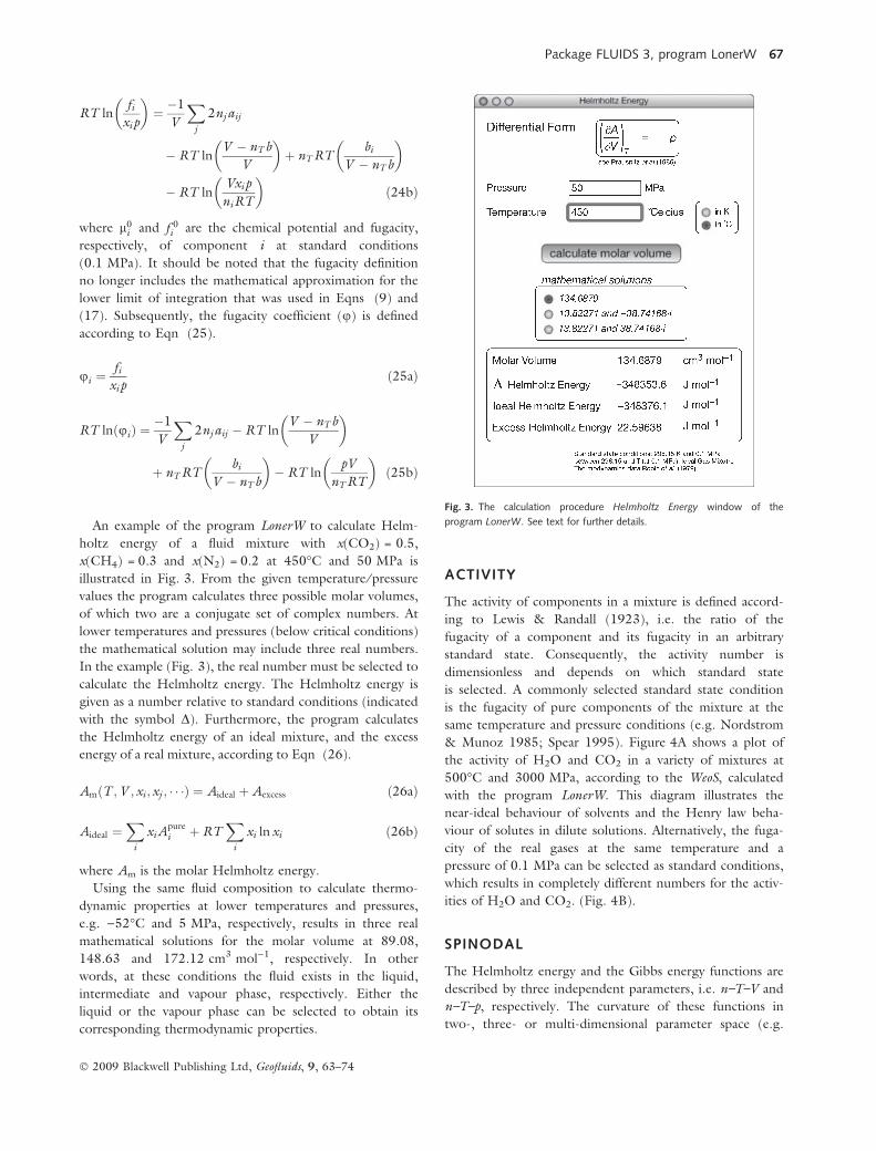
Figure 5 illustrates the spinodal of a binary H2O–CO2

fluid mixture with x(CO2) = 0.1 calculated with WeoS. The

spinodal has a small loop near the critical point of this fluid

mixture and it clearly differs from the binodal, which is

also known as the dew curve and the bubble curve. The

spinodal extends into that part of the diagram which has

negative pressures, whereas the binodal remains within the

positive pressure part.

CRITICAL POINT

The critical point, also known as the plait point (see e.g.

Korteweg 1903) marks the highest temperature and pres-

sure that boiling can occur in a pure system. Beyond the

critical point, i.e. at higher temperatures and pressures, the

fluid is in a homogeneous supercritical state. Every fluid

mixture with a specific composition has a critical point. In

binary mixtures, the critical points of all possible composi-

tions can be represented by a critical curve or locus of criti-

cal points. The critical point can be obtained from the

Helmholtz energy function (e.g. Baker & Luks 1980; van

Konynenburg & Scott 1980), and it marks that part of this

surface where the two inflexion points of the spinodal

coincide (see previous paragraph). Therefore, the condi-

tions for the spinodal calculation (Eqn 28) are also applied

to the critical point. In addition, the critical curve of

multi-component fluid mixtures is also defined by the

determinant (Dcrit) of the following matrix:

Dcrit ¼

AVV An1V An2V � � �AVn1

An1n1An2n1

� � �... ..

. ... ..

.

DV Dn1Dn2

. ..

��

��¼ 0 ð31Þ

The matrix in Eqn (31) is square and contains q col-

umns, where q is the number of differentiation variables,

i.e. volume and number of components minus 1 (c.f. Eqn

28). The number of rows is defined according to the dif-

ferentiation variables volume and number of components

minus 2, and the last row is reserved for the partial deriva-

tives of the determinant Dspin from Eqn (28):

DV ¼oDspin

oV

� �ð32aÞ

Dn1¼ oDspin

on1

� �ð32bÞ

Dn2¼ oDspin

on2

� �ð32cÞ

The derivatives of the spinodal determinant (see also

Baker & Luks 1980) are calculated from the sum of the

element-by-element products of the matrix of cofactors (or

adjoint matrix) of the spinodal (Eqn 33) and the matrix

of third derivatives of the Helmholtz energy function

(Eqn 34).

CVV Cn1V Cn2V � � �CVn1

Cn1n1Cn2n1

� � �CVn2

Cn1n2Cn2n2

� � �... ..

. ... . .

.

��

��ð33Þ

where Cxy are the individual elements in the matrix of

cofactors, as obtained from the Laplacian expansion.

AVVK An1VK An2VK � � �AVn1K An1n1K An2n1K � � �AVn2K An1n2K An2n2K � � �

..

. ... ..

. . ..

��

��ð34Þ

where the subscript K refers to the variable that is used in

the third differentiation, i.e. volume and amount of sub-

stance of the components 1 and 2, as indicated in Eqn

(32a), (32b) and (32c), respectively. For example, in unary

Fig. 5. Temperature–pressure diagram of a binary fluid mixture of H2O and

CO2 with x(CO2) = 0.1, calculated according to van der Waals (1873). The

dashed curve is the spinodal (spin), the shaded area are T–p conditions of

immiscibility, which is limited by the isopleth (bin, i.e. dew curve, critical

point and bubble curve). The isochore 60.8013 cm3 mol)1 is illustrated

(isoc) that crosses the isopleth at hom (homogenization conditions). The

metastable extension of this isochore towards the spinodal is illustrated with

isoc‘‘. nuc is the intersection of isoc’’ and the spinodal and reflects the

minimum nucleation temperature of a vapour bubble in the fluid inclusion.

isoc‘‘ is the stable continuation of isoc in the two-phase field.



and binary fluid systems, the determinant of Eqn (31) is

given by Eqn (35a) and (35b), respectively.

AVVV ¼ 0 ð35aÞ

� An1n1�An1Vð Þ �AVVV þ An1n1

�AVV þ 2A2n1V

� ��An1VV

� 3 � An1V �AVVð Þ �An1n1V þ A2VV

�An1n1n1

¼ 0 ð35bÞ

As with Eqn (28), to reduce computation time in the

program LonerW, the LU decomposition has been used to

calculate the determinant in Eqn (31). In conclusion, the

two determinants given in Eqns (28) and (31) are used to

calculate the critical point of any fluid mixture. However,

the computation time is significantly increased for mixtures

containing more than seven components.

The example in Fig. 5 illustrates the critical point of a

fluid mixture of x(CO2) = 0.1 and x(H2O) = 0.9 at

338.085�C and 21.39 MPa with a molar volume of

90.2345 cm3 mol)1, as obtained from the WeoS. This

point is located on both the spinodal (obtained from Eqn

28) and the binodal, i.e. the boundary T–p conditions of

phase separation.

PSEUDO-CRITICAL POINT

The pseudo-critical conditions are defined according to a

different concept to the critical point (see previous para-

graph) and are directly obtained from the mathematical

equation that defines pressure (Eqn 3):

op

oV

� �T ;n

¼ 0 ð36aÞ

o2p

oV 2

� �T ;n

¼ 0 ð36bÞ

In pure systems, the pseudo-critical conditions are equal

to the critical point calculation described in the previous

section (Eqns 28 to 35). In fluid mixtures, the pseudo-

critical point always underestimates the true critical point

in temperature and pressure. These conditions have been

used in literature to relate directly the true critical point

conditions to the a and b parameter in Eqn (3), and they

are the principles of the corresponding state theory (e.g.

van der Waals 1880; Pitzer 1939).

vpc ¼ 3b ð37aÞ

ppc ¼a

27b2ð37bÞ

Tpc ¼8a

27bRð37cÞ

Alternatively, the a and b parameters can be replaced by

the critical values of pure systems (Eqn 38).

a ¼ 27

64�R

2T 2c

pcð38aÞ

b ¼ 1

8�RTc

pcð38bÞ

The true critical molar volume of pure systems is not

included in the calculations in Eqn (36). In general, the

mathematically obtained critical molar volume differs sig-

nificantly from the measured critical molar volume, which

illustrates the deficits in the mathematical formulation of

this equation of state at near critical conditions. For exam-

ple, the critical conditions of pure CO2 are 30.978�C,

7.3773 MPa and 94.118 cm3 mol)1 (Span & Wagner

1996). A critical molar volume of 128.536 cm3 mol)1 is

calculated from the critical temperature and pressure

according to Eqns (37) and (38).

HOMOGENIZATION CONDITIONS

Microthermometry is of major importance for the analyses

of fluid inclusions. The homogenization conditions of

liquid and vapour phases, also known as bubble point and

dew point, in the inclusions can be directly used to calcu-

late bulk-fluid densities and to define isochores and trap-

ping conditions (e.g. Shepherd et al. 1985). Each equation

of state can be used to perform these calculations; how-

ever, most equations have not been designed for these

types of analyses. Thermodynamically, and for calculation,

homogenization is defined as the point at which the fugac-

ities of each component in both phases are equal (e.g.

Prausnitz et al. 1980; Bakker 2003) (Eqn 39).

fvap

i ¼ fliq

i ð39Þ

The fugacities in both phases are calculated with the

same equation of state, according to Eqns (24) and (25).

At equilibrium conditions, temperature and pressure of

both phases are equal, whereas the molar volume of the

liquid phase is clearly different from that of the vapour

phase. The program LonerW allows the calculation of

homogenization conditions (Fig. 6) with WeoS. Usually,

homogenization temperatures are measured, which can be

input directly in the procedure window Bubble-Dew Point

(Fig. 6). In addition, homogenization pressure can also be

input for experimental mathematical analyses. Fluid inclu-

sions may homogenize into the liquid phase (at the bubble

curve) or in to the vapour phase (at the dew curve), which

has to be specified in the program, i.e. the mode of

homogenization (Fig. 6). Critical homogenization is best

analysed by selecting the calculation procedure Critical

Point. The next step in the procedure is to calculate a first

approach, because the complexity of mathematical model-

70 R. J. BAKKER


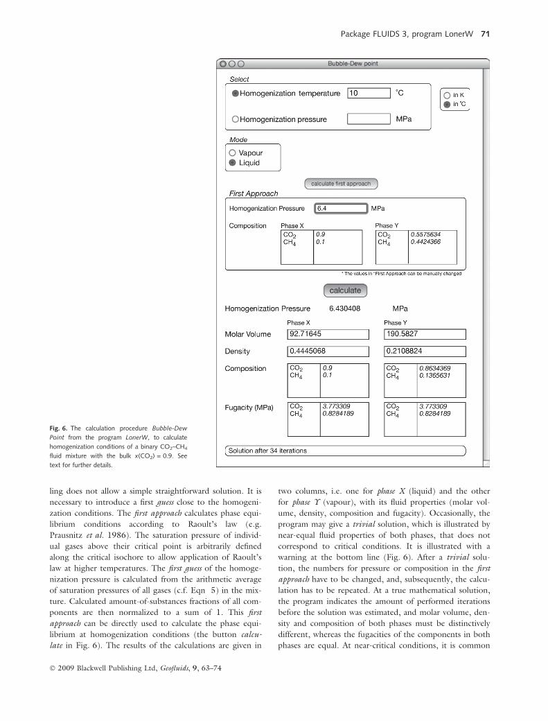
ling does not allow a simple straightforward solution. It is

necessary to introduce a first guess close to the homogeni-

zation conditions. The first approach calculates phase equi-

librium conditions according to Raoult’s law (e.g.

Prausnitz et al. 1986). The saturation pressure of individ-

ual gases above their critical point is arbitrarily defined

along the critical isochore to allow application of Raoult’s

law at higher temperatures. The first guess of the homoge-

nization pressure is calculated from the arithmetic average

of saturation pressures of all gases (c.f. Eqn 5) in the mix-

ture. Calculated amount-of-substances fractions of all com-

ponents are then normalized to a sum of 1. This first

approach can be directly used to calculate the phase equi-

librium at homogenization conditions (the button calcu-

late in Fig. 6). The results of the calculations are given in

two columns, i.e. one for phase X (liquid) and the other

for phase Y (vapour), with its fluid properties (molar vol-

ume, density, composition and fugacity). Occasionally, the

program may give a trivial solution, which is illustrated by

near-equal fluid properties of both phases, that does not

correspond to critical conditions. It is illustrated with a

warning at the bottom line (Fig. 6). After a trivial solu-

tion, the numbers for pressure or composition in the first

approach have to be changed, and, subsequently, the calcu-

lation has to be repeated. At a true mathematical solution,

the program indicates the amount of performed iterations

before the solution was estimated, and molar volume, den-

sity and composition of both phases must be distinctively

different, whereas the fugacities of the components in both

phases are equal. At near-critical conditions, it is common

Fig. 6. The calculation procedure Bubble-Dew

Point from the program LonerW, to calculate

homogenization conditions of a binary CO2–CH4

fluid mixture with the bulk x(CO2) = 0.9. See

text for further details.



for the calculation to reach a trivial solution, and the first

approach has to be very close to the real solution. In addi-

tion, the procedure Critical Point can be used to estimate

those near-critical conditions that have to be introduced in

the first approach.

All possible homogenization conditions of a binary

H2O–CO2 fluid mixture with x(CO2) = 0.1, also known is

an isopleth are illustrated in Fig. 5. Within the shaded enve-

lope, indicated with bin (Fig. 5), this fluid is unmixed in

coexisting vapour and liquid phases. The figure shows an

isochore calculated for a homogeneous mixture with a molar

volume of 60.8013 cm3 mol)1. An inclusion with these

liquid-like fluid properties must nucleate a vapour bubble

(phase separation) on entering into the envelope at 290�C(hom in Fig. 5). However, nucleation can be inhibited

before the spinodal curve is intersected by this isochore.

Consequently, the fluid inclusion can cool along this isochore

down to 238.78�C and 2.183 MPa (nuc in Fig. 5) without

the formation of a vapour bubble. At nucleation, the fluid

system changes abruptly into a stable phase assemblage, at

higher pressures (11.029 MPa) and within the isopleth.

LIQUID–VAPOUR EQUILIBRIA

Fluid inclusions, which contain a vapour bubble in a liquid

phase, are thermodynamically considered at liquid–vapour

equilibrium conditions. The properties of both phases are

calculated according the fugacity equalities from Eqn (39)

in the procedure Liquid-Vapour Equilibrium in the pro-

gram LonerW (Fig. 7). The fluid properties of inclusions

with known bulk composition and molar volume (density),

as obtained from e.g. homogenization conditions from the

procedure Bubble-Dew Point (see previous paragraph), can

be calculated below their homogenization conditions. The

Fig. 7. The calculation procedure Liquid-Vapour

Equilibrium from the program LonerW, to

calculate the properties of coexisting liquid and

vapour phase at 0�C, the bulk fluid (i.e. of a

homogeneous fluid) is a binary CO2–CH4

mixture with x(CO2) = 0.9 and a molar volume

of 92.71645 cm3 mol)1. See text for further

details.

72 R. J. BAKKER


program calculates volume fractions of the coexisting

phases, in addition to molar volume, density, composition

and fugacity of the liquid and vapour phase at equilibrium

conditions (Fig. 7). Consequently, the program permits

the calculation of the continuation of bulk isochores of

fluid mixtures in inclusions below homogenization condi-

tions. Similar to the procedure Bubble-Dew Point, the cal-

culations have to start with a first approach (Fig. 7), in

which pressure, volume fractions and composition can be

manually varied to obtain a mathematical solution.

Figure 5 illustrates the isochore calculated with LonerW

within the phase-separation field (isoc¢ in Fig. 5) of the

x(CO2) = 0.1, H2O–CO2 fluid mixture, which ends at the

bubble curve (homogenization conditions). Per definition,

this isochore cannot be traced outside this field of immisci-

bility towards lower temperatures. Along this curve, the vol-

ume fraction of the vapour bubble and the properties of

both liquid and vapour phase vary with decreasing tempera-

ture. For example, the volume fraction of the vapour bubble

is 0.214 at the nucleation temperature 238.78�C and

11.029 MPa (Fig. 5). The fluid properties of the vapour are

268.94 cm3 mol)1 and x(CO2) = 0.2222, and those of the

liquid are 50.22 cm3 mol)1 and x(CO2) = 0.0668.

CONCLUSIONS

The program group Loners from the computer package

FLUIDS (Bakker 2003) have been revised and furnished

with a new user interface (Graphical User Interface,

REALBasic 2007). The equation of state according to

van der Waals (1873) has been added to the list of pro-

grams in the Loners group with the name LonerW. This

equation of state is used to illustrate all possible calcula-

tion procedures to obtain thermodynamic properties of

fluid mixtures, including: (i) molar volume; (ii) pressure;

(iii) temperature; (iv) fugacity; (v) activity; (vi) homogeni-

zation conditions; (vii) liquid–vapour equilibrium; (viii)

spinodal; (ix) critical point; (x) internal energy; (xi)

enthalpy; (xii) entropy; (xiii) Helmholtz energy; (xiv)

Gibbs energy; (xv) chemical potentials. This type of revi-

sion will be applied to all the equations of state included

in the group Loners.

Experimental mathematical calculations can be performed

with the program LonerW to obtain the fluid properties of

hypothetical systems. It can also be used to interpret micro-

thermometric data from fluid inclusions and to interpret

general pore fluid properties. The validity of this equation of

state can be tested by direct comparison with experimental

data for many thermodynamic parameters.

The program has been compiled for three different com-

puter operating systems: Mac Os X (PowerPC and Intel),

Microsoft Windows (2000, XP and Vista), and Linux

(GTK+ 2.x), and it can be downloaded from the website:

http://fluids.unileoben.ac.at/Computer.html

ACKNOWLEDGEMENTS

I greatly appreciate the comments and suggestions of two

anonymous reviewers.

REFERENCES

Baker LE, Luks KD (1980) Critical point and saturation pressure

calculations for multipoint systems. Society of Petroleum Engi-neers Journal, 20, 15–24.

Bakker RJ (2003) Package FLUIDS 1. Computer programs foranalysis of fluid inclusion data and for modelling bulk fluid

properties. Chemical Geology, 194, 3–23.

Bakker RJ, Brown PE (2003) Computer modelling in fluid

inclusion research. In: Fluid Inclusions, Analysis and Interpre-tation (eds Samson I, Anderson A, Marshall D), pp. 175–

212. Short Course, Mineralogical Association of Canada,

Ottawa, Canada.

Beyer WH (1991) CRC Standard Mathematical Tables and For-mulae, 29th edn. CRC Press, Boca Raton, FL, pp. 609.

Diamond LW (2003) Introduction to gas-bearing, aqueous fluid

inclusions. In: Fluid Inclusions, Analysis and Interpretation (edsSamson I, Anderson A, Marshall D), pp. 101–58. Mineralogical

Association of Canada, Short Course.

Driesner T, Heinrich CA (2006) The system H2O-NaCl. Part 1:

Correlation formulae for phase relations in the temperature-pressure-composition space from 0 to 1000 �C, 0 to 5000 bar,

a 0 to 1 XNaCl. Geochimica et Cosmochimica Acta, 71, 4880–

901.

Haar L, Gallagher JS, Kell GS (1984) NBS ⁄ NRC Steam Tables.Hemisphere Publishing Corporation, Washington, DC.

Holloway JR (1977) Fugacity and activity of molecular species in

supercritical fluids. In: Thermodynamics in Geology (ed. FraserDG), pp. 161–82. Nato Advanced Study Institute Series.

Series C: Mathematical and Physical Science, Oxford, UK.

Horn RA, Johnson CR (1985) Matrix Analysis. Cambridge Uni-

versity Press, Cambridge.van Konynenburg PH, Scott RL (1980) Critical lines and

phase equilibria in binary van der Waals mixtures. Philosophi-cal Transactions of the Royal Society of London, 298, 495–

540.Korteweg DJ (1903) Plaitspoints and corresponding plaits in the

neighborhood of the sides of the w-surface of Van der Waals.

Proceedings of the Section of Sciences, Koninklijke NederlandseAkademie van Wetenschappen, 5, 445–65.

van Laar JJ (1905) An exact expression for the course of the spin-

odal curves and of their plaitpoints for all temperatures, in the

case of mixtures of normal substances. Proceedings of the RoyalAcademy of Amsterdam, 7, 646–57.

Levelt-Sengers J (2002) How Fluids Unmix, Discoveries by theSchool of Van der Waals and Kamerlingh Onnes. Koninklijke

Nederlandse Akademie van Wetenschappen, Amsterdam, pp302.

Lewis GN, Randall M (1923) Thermodynamics and the FreeEnergy of Chemical Substances. McGraw-Hill, New York, pp

653.Lorentz HA (1881) Uber die Anwendung des Satzes vom Virial

in den kinetischen Theorie der Gase. Annalen der Physik, 12,

127–36.Nordstrom DK, Munoz JL (1985) Geochemical Thermodynamics.

The Benjamin ⁄ Cummings Publishing Co., Inc., Menlo Park,

CA, pp 477.



Pitzer KS (1939) Corresponding states for perfect liquids. Journalof Chemical Physics, 7, 583.

Prausnitz JM, Anderson TF, Grens EA, Eckert CA, Hsieh R,

O’Connell JP (1980) Computer Calculations for the Multicompo-nent Vapor-Liquid and Liquid-Liquid Equilibria. Prentice-Hall,Englewood Cliffs, NJ.

Prausnitz JM, Lichtenthaler RN, Gomes de Azevedo E (1986)

Molecular Thermodynamics of Fluid-phase Equilibria, 2nd edn.Prentice-Hall Inc., Englewood Cliffs, NJ, pp 600.

Robie RA, Hemingway BS, Fisher JR (1979) Thermodynamic

properties of minerals and related substances at 298.15 K and

1 bar (105 Pascal) pressure and at higher temperatures. Geologi-cal Survey Bulletin, 1452, US Government Printing Office,

Washington, DC.

Shepherd TJ, Rankin AH, Alderton DHM (1985) A PracticalGuide to Fluid Inclusion Studies. Blackie, Glasgow, pp 239.

Span R, Wagner W (1996) A new equation of state for carbon

dioxide covering the fluid region from the triple-point tempera-

ture to 1100 K at pressures up to 800 MPa. Journal of Physicaland Chemical Reference Data, 25, 1509–96.

Spear FS (1995) Metamorphic Phase Equilibria and Pressure–Tem-perature–Time Paths. Monograph Series, Mineralogical Society

of America, Washington, DC, pp 799.van der Waals JD (1873) De continuiteit van den gas - en vloeistof-

toestand. PhD Thesis, Universiteit Leiden, pp 134.

van der Waals JD (1880) Over d coefficienten van uitzetting en

van samendrukking in overeenstemmende toestanden der ver-schillende vloeistoffen. Verhandelingen der Koninklijke Akade-mie van Wetenschappen, 20.

van der Waals JD (1890) Molekulartheorie eines Korpers, der auszwei verschiedenen Stoffen besteht. Zeitschrift fur physikalischeChemie, 5, 133–73.

APPENDIX

The partial derivatives of the Helmholtz energy in respect

to total volume and amount of substance, as obtained from

the WeoS.

AV ¼oA

oV

� �ni ;nj ;...

¼ n2T a

V 2� nT RT

V � nT b¼ �p ðA1Þ

Ani¼ oA

oni

� �V ;nj

¼ðu0i �Ts0

i Þ�2

V

Xj

nj aij�RT lnV�nT b

V

� �

þnT RTbi

V�nT b�RT ln

V

niRT

� ��1

� �¼�i ðA2Þ

AVV ¼o2A

oV 2

� �ni ;nj ...

¼ �2n2

T a

V 3þ nT RT

V � nT bð Þ2ðA3Þ

Ani ni¼ o2A

on2i

� �V ;nj

¼ � 2

Vaii þ 2RT

bi

V � nT b

þ nT RTb2

i

V � nT bð Þ2þRT

niðA4Þ

Ani nj¼ o2A

oninj

� �V

¼ � 2

Vaij þ RT

ðbi þ bj ÞV � nT b

þ nT RTbibj


AVni ¼o2A

oV oni

� �nj

¼ 2

V 2

Xj

nj aij �RT

V � nT b

� nT RTbi


AVVV ¼o3A

oV 3

� �n

¼ 6n2

T a

V 4� 2nT RT

1


Aninini ¼o3A

on3i

� �V ;nj

¼ 2RTb2

i

V � nT bð Þ2

þ 2nT RTb3

i

V � nT bð Þ3�RT

n2i

ðA8Þ

Ani nj nk¼ o3A

onionj onk

� �V

¼ RTðbi þ bj Þbk

V � nT bð Þ2

þ 2nT RTbibj bk


AniVV ¼o3A

onioV 2

� �

¼ � 4

V 3

Xj

nj aij þRT1

V � nT bð Þ2

þ 2nT RTbi


AniniV ¼o3A

on2i oV

� �

¼ 2

V 2aii �RT

2bi

V � nT bð Þ2

� 2nT RTb2

i


Aninj V ¼o3A

onionj oV

� �

¼ 2

V 2aij �RT

ðbi þ bj ÞV � nT bð Þ2

� 2nT RTbibj


74 R. J. BAKKER


Documents

Package FLUIDS. Part 3: correlations between equations of