Pacific Gas and Electric Company - BASE Energy, Inc. Report - Wine Stabilization... · Pacific Gas and Electric Company Emerging Technologies Program Application Assessment Report

Pacific Gas and Electric Company

Emerging Technologies Program

Application Assessment Report No. 0612

Wine Stabilization through Electrodialysis

Issued: May 2007 Project Manager: Steve Fok Pacific Gas and Electric Company Prepared by: Ricardo A. Sfeir Sandra Chow Electrical Engineer Mechanical Engineer BASE Energy, Inc. BASE Energy, Inc.

Pacific Gas & Electric Company Emerging Technologies Program

Legal Notice This report was prepared by Pacific Gas and Electric Company for exclusive use by its employees and agents. Neither Pacific Gas and Electric nor any of its employees and agents: 1) makes any written or oral warranty, expressed or implied, including, but not limited to those

concerning merchantability or fitness for a particular purpose; 2) assumes any legal liability or responsibility for the accuracy, completeness, or usefulness of

any information, apparatus, product, process, method, or policy contained herein; or 3) represents that its use would not infringe any privately owned rights, including, but not

limited to, patents, trademarks, or copyrights.

Electrodialysis Wine Stabilization B A S E

i


Table of Contents 1. EXECUTIVE SUMMARY .................................................................................................. 1

1.1. Objective of Study .......................................................................................................... 1 1.2. Major Conclusions .......................................................................................................... 1 1.3. Key Findings................................................................................................................... 2

2. PROJECT BACKGROUND................................................................................................ 3 2.1. Wine Stabilization........................................................................................................... 3 2.2. Technologies for Cold Stabilization Enhancement......................................................... 3 2.3. Metric for Cold Stabilization .......................................................................................... 4 2.4. Application of Electrodialysis for Wine Stabilization .................................................... 5

3. FIELD EVALUATIOIN OF ENERGY CONSUMPTION OF ELECTRODIALYSIS AND COLD STABILIZATION......................................................................................... 6

3.1. Overall Measurement Plan.............................................................................................. 6 3.2. Description of the Site .................................................................................................... 8 3.3. Instrumentation and Measurement Systems ................................................................. 11

4. RESULTS ............................................................................................................................ 13 4.1. Cold Stabilization Measurements and Analysis ........................................................... 13 4.2. Electrodialysis Measurements and Analysis................................................................. 16 4.3. Limitations on Energy and Demand Savings................................................................ 17 4.4. Summary of Energy and Demand Savings ................................................................... 17

5. CONCLUSIONS ................................................................................................................. 19 6. APPENDIX.......................................................................................................................... 20

6.1. Thermodynamic Model for Cold Stabilization............................................................. 20 6.2. Project Timeline and Key Dates ................................................................................... 21 6.3. Equations Used for Thermodynamic Model Analysis.................................................. 22 6.4. Spreadsheet Snapshots of Thermodynamic Model Analysis........................................ 31 6.5. Graphs of Data Recorded During Cold Stabilization and Electrodialysis Tests .......... 35


ii


1. EXECUTIVE SUMMARY

1.1. Objective of Study Assess the electrical energy and demand savings that could result from using an Electrodialysis System in place of cold stabilization of wine.

1.2. Major Conclusions Implementing electrodialysis wine stabilization instead of traditional cold stabilization (without enhancement) may result in significant electrical energy savings. Another non-energy related advantage of electrodialysis technology is an increase in stabilization rate, reducing the stabilization time of traditional cold stabilization of typically weeks to a few days. However, this study shows that electrodialysis technology results in an increase in water consumption as well as the resulting wastewater which would need to be treated. Table 1-1 compares the performance of cold stabilization with electrodialysis stabilization.

TABLE 1-1 COLD VS ELECTRODIALYSIS WINE STABILIZATION Stabilization Method Cold Stabilization Electrodialysis Stabilization Energy Consumption 26,891 kWh 165 kWh Average Demand 24 kW 5 kW Increase in Water Consumption 0 gallons 3,010 gallons Adjusted Energy Consumption* 22,965 kWh 170 kWh Stabilization Period 1,108 hours 31 hours Initial Conductivity Drop 14.8% 14.6% Final Conductivity Drop 3.4% 2.5% Volume of Stabilized Wine 18,500 gallons 21,500 gallons Energy Intensity 1,200 Wh/gal 7.9 Wh/gal

* The adjusted cold stabilization energy consumption considers the added tank and bare pipe insulation. The adjusted electrodialysis stabilization energy consumption considers the extra energy needed for wastewater treatment. The energy consumption for the increased electrodialysis water consumption is based on the Secondary Wastewater Treatment (activated sludge system) Baseline Study. Table 1-2 summarizes the type of wine that was tested in this study as well as some background information regarding the tanks that the wine was cold stabilized in.


1


TABLE 1-2 INFORMATION REGARDING WINE AND TANKS IN STUDY

Parameter Tank 952 Tank 953 Wine Variety Tested 2006 Pinot Grigio 2006 Pinot Grigio Initial Volume of Wine 9,250 gallons 8,813 gallons

Type of Tank Uninsulated, jacketed stainless steel tank

Uninsulated, jacketed stainless steel tank

Tank Capacity 9,250 gallons 9,250 gallons Tank Location Indoor Indoor

1.3. Key Findings After analyzing the collected data it was determined that:

1. Electrodialysis Stabilization may result in significant electrical energy savings (approximately 99% savings)

2. Electrodialysis Stabilization may result in significant demand savings (approximately 79% reduction in demand)

3. A significant portion of the energy used in Cold Stabilization may be due to the chemistry of crystallization and the resulting interactions between the ions and complexing factors.


2


2. PROJECT BACKGROUND

2.1. Wine Stabilization Wine stabilization as part of the winemaking process reduces the concentration of potassium bitartrate (cream of tartar) in wine. Traditionally, wineries lower the potassium bitartrate solubility in wine by chilling the wine to approximately 27 ºF. Wines are typically maintained at this temperature for a period of 1.5 to 3 weeks, depending on how easy it is to crystallize the potassium bitartrate, i.e. how “stable” the wine is. Several factors can influence the crystallization rate of potassium bitartrate, among them1:

• Nucleation: the number of nuclei on which crystals can form and grow. • Diffusion: the rate at which the dissolved potassium bitartrate comes into contact with the

crystal formations. • The rate at which crystals grow. • Grape variety.

Once the desired potassium bitartrate concentration is achieved, the wine is filtered and pumped to holding tanks, ready to be bottled.

2.2. Technologies for Cold Stabilization Enhancement There are different kinds of cold stabilization enhancement that may expedite the process1. One variation of this process is the Contact Process, where the chilled wine is seeded with potassium bitartrate and mixed into the wine. Mixing in the potassium bitartrate seeds hastens the crystallization rate in the wine. The crystals left behind after wine filtration can be ground and reused to seed the next batch. Another variation of cold stabilization is the Filtration Process, where wine is filtered through a potassium bitartrate bed. As wine flows through the bed, the potassium bitartrate in the wine crystallizes in the filter bed. Wine may be passed through the crystal bed several times, until wine is stabilized. A third variation of cold stabilization is the Crystal Flow Process. This process involves chilling the wine to temperatures between 14 ºF and 21 ºF (freezing point of wine). Freezing the wine will generate potassium bitartrate and ice crystals. These crystals act as nuclei for further crystal growth. This process requires using scraped-surface heat exchangers.

1 Refrigeration for Winemakers, Ray White, Ben Adamson, Bryce Rankine, Winetitles, Winemaking Series, 1998


3


2.3. Metric for Cold Stabilization There are various methods used to determine wine stability with respect to potassium bitartrate crystallization and they vary depending on the winemaker. Some of these methods include:

• Chill proofing followed by a Concentration Product (CP) Test • Chill proofing followed by visual inspection • Filtering at 25 ºF for 24 hours followed by visual inspection • Wine freeze/slush test • Conductivity test

The stability test used in this study is the Conductivity Test and is described below. Conductivity Test: The conductivity test is performed by taking a wine sample from the stabilization tank. Throughout the test, the wine sample is maintained at the lowest temperature that the wine is expected to encounter. The sample wine is mixed and its conductivity is recorded. The sample is then seeded with potassium bitartrate (KHT) and mixed. Wine conductivity is measured and logged (approximately every 1 to 2 minutes) for a period of approximately 30 minutes. If the final conductivity value varies by less than 5% compared to the initial conductivity value, the wine is determined to be stable. Typically, stable dry white wines will have conductivities between 1,400 and 1,600 micro-Siemens per centimeter (μS/cm)2.

2 A Review of Potassium Bitartrate Stabilization of Wines, Bruce Zoecklein, Department of Horticulture, Virginia Polytechnic Institute and State University, 1998


4


2.4. Application of Electrodialysis for Wine Stabilization Electrodialysis (ED) process, used for wine stabilization, removes the tartaric acids from the wine by passing it through an electric field and collecting ions (potassium (K+), calcium (Ca++) and negatively charged tartaric acids) on anionic and cationic membranes.

K+

Ca++

TA- TA-

K+

Ca++

AnionicMembrane

CationicMembrane

AnionicMembrane

Compartment #1Wine

Compartment #2Extraction Salts

+

Anode

-

Cathode

TA- = Negatively charged tartaric acid.

Figure 2-1 Simplified Schematic of Ion Extraction on the Electrodialysis Process3

Inside the ED system there are two chambers separated by a cationic membrane. The first chamber holds the wine; the second chamber contains a solution of potassium and calcium ions that have been extracted by applying an electric field across the wine. Water flows through the second chamber creating a brine solution made up of the potassium and calcium ions. Jean-Louis Escudier (2002) shows a simplified schematic of ion migration within a single cell, which is reproduced in Figure 2-1. Figure 2-1 shows that the potassium and calcium ions migrate from Compartment #1 to Compartment #2 within its own cell, however the Tartaric Acid migrates from Compartment #1 to Compartment #2 of an adjacent cell. Each cell has an electric potential drop of approximately 1 Volt.

3 Vinidea.net – Wine Internet Technical Journal, 2002, No. 4; Ecudier- Electrodialysis – Article 4 of 5


5


3. FIELD EVALUATIOIN OF ENERGY CONSUMPTION OF ELECTRODIALYSIS AND COLD STABILIZATION

3.1. Overall Measurement Plan This study compares the electrical energy consumption of traditional wine stabilization (cold stabilization) to that of electrodialysis wine stabilization. Wine from the same batch (2006 Pinot Grigio) was processed through cold stabilization and electrodialysis stabilization. Each system processed approximately 20,000 gallons of wine. Electrical energy consumption, temperatures, timing of equipment, wine tank levels, water consumption, flow rates and wine conductivity were monitored and logged for the duration of the study (from January through April 2007). A detailed description of measurement points for each system is described in the Instrumentation and Measurement Systems in Section 3.3. To accurately compare the electrical energy consumption of both systems, it was determined when wine conductivity reached 2.5%, the wine would be considered stable and data logging would be stopped. As a baseline, the project considers a dedicated chiller system supplying chilled glycol to cool two 9,250 gallon tanks (cold stabilization). Glycol is chilled through a 40 hp water cooled reciprocating compressor and pumped to the stabilization tanks. The chiller compressor and condenser are located outdoors in a pad beside the Barrel Room. The two 9,250 gallon un-insulated stabilization tanks are located inside the Barrel Room which is maintained at approximately 50º F. The baseline used for the study considers cold stabilization in its most basic form, with no mixing, seeding or any stabilization “enhancement.” A simplified schematic of the cold stabilization system is shown in Figure 3-1 on the following page. The specifications for the refrigeration system used for cold stabilization are shown in Table 3-1. The tested electrodialysis system is a portable system mounted into a trailer (model STARS ED-600 by Winesecrets). The trailer was “plugged” to an electrical outlet inside one of the tank rooms. Wine is pumped from the fermentation tanks to the ED trailer and processed through as many loops as necessary to reach the desired wine conductivity. Once the target conductivity is reached, wine is pumped to a holding tank, ready for bottling. In addition to the wine recirculation pump used in the ED system, water pumps are used to move the brine solution and wash the membranes once a batch is done. The ED system requires three water lines: a hard water line, a hot water line and a soft water line. A simplified schematic of the ED system is shown in Figure 3-2 on the following page.

TABLE 3-1 COLD STABILIZATION EQUIPMENT Equipment Manufacturer Model Motor(s) (hp) Refrigeration Compressor Carlyle 5H40-149 40 Glycol Pump ITT Bell & Gossett 5 Cooling Tower Evapco LSOB41 5 (fan) and 3/4 (pump) Condenser Water Pump 1


6


Outdoor Chiller Pad

Barrel Room

CoolingTower

CondenserPump

Chiller

Glycol SupplyPump

GlycolReturnTank

StabilizationTanks

Figure 3-1 Simplified Schematic of the Cold Stabilization System

FermentationTank

Wine TransferPump

ED System

Wine TransferPump

HoldingTank

Hard, Soft andHot Water Lines

ED Trailer

Wastewater

Figure 3-2 Simplified Schematic of the Electrodialysis System


7


3.2. Description of the Site The study was hosted by a winery located in Northern California. As stated earlier, the uninsulated tanks used for cold stabilization were located inside the Barrel Room. Figure 3-3 below shows the iced tanks. The blue “colored” ice is due to a minor glycol leak from the refrigeration system.

Figure 3-3 Uninsulated Cold Stabilization Tanks

The chiller, compressor and cooling tower were located on a pad outside the Barrel Room. Figure 3-4 shows the cooling tower as well as the 40 hp reciprocating refrigeration compressor. To the left of the refrigeration compressor is the glycol return tank and behind it (not shown) the glycol supply pump. Ice buildup can be seen on the uninsulated pipe section coming right out of the refrigeration compressor, before pipe insulation begins.


8


Figure 3-4 Refrigeration System used for Cold Stabilization

Finally, the portable electrodialysis system (inside the trailer) is shown in Figure 3-5. On the right side is one of the temperature sensors and data loggers used to record the wine temperature as it comes into the electrodialysis machine. The three cylindrical shapes at the center are pumps used to circulate the wine within the electrodialysis machine, and pumps used to circulate water. On the far back (behind the blue hoses) are the electrodialysis membranes where the electric field is applied. On the other side of the machine (behind the pumps) are two wine holding tanks. Finally, tied around the middle pump, is a motor On/Off data logger.


9


Figure 3-5 Electrodialysis System


10


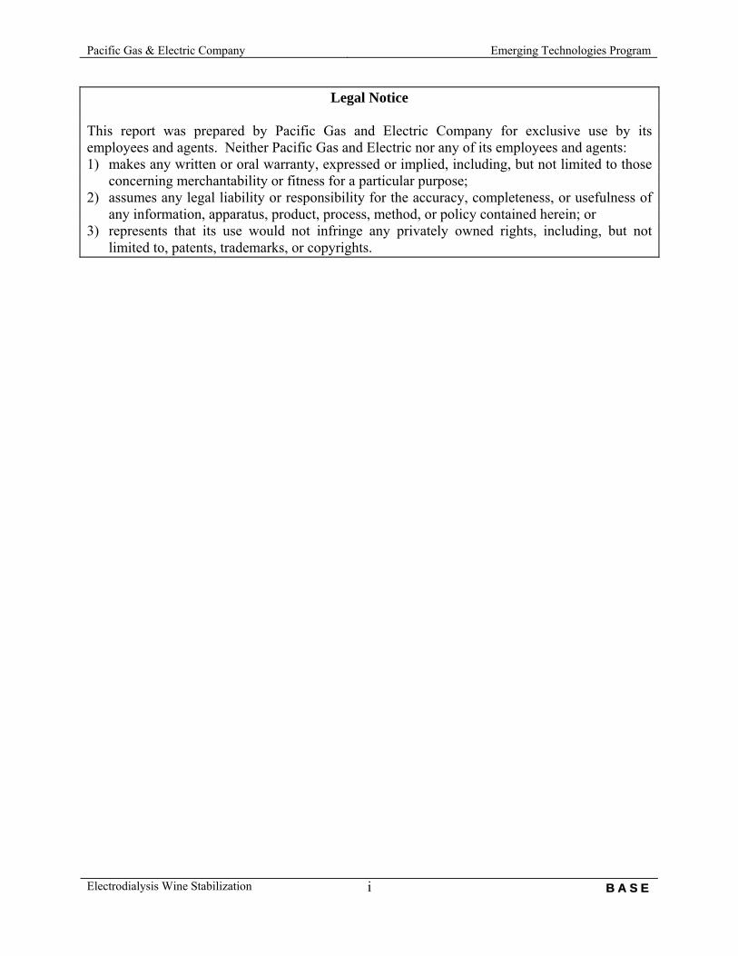
3.3. Instrumentation and Measurement Systems The following equipment was used to log the parameters needed for the present analysis:

• Electrical Energy Consumption and Power: o DENT ElitePro Logger with current transducer o AEMC Instruments Model 3910

• Temperature: o PACE XR440 Pocket Logger with thermistor sensor o HOBO H08-032-08 Pro RH/TEMP

• Equipment On/Off Status: o DENT TOUM MagLogger o HOBO U12-008 Industrial data logger with current transducer

• Flow Meter: o Controlotron 1010WDP1 with clamp-on ultrasonic sensor

In addition, the winery personnel helped record, throughout the duration of the study, the following data:

• Wine temperature in the cold stabilization tanks • Cold stabilization tank level • Cold stabilization wine conductivity • Cold stabilization wine pH • Water consumption of the ED system • Starting and Finishing conductivity for electrodialysis stabilized wine.

Tables 3-2 and 3-3 identify the measurement points for the Electrodialysis and Cold Stabilization systems, respectively.

TABLE 3-2 ELECTRODIALYSIS STABILIZATION MEASUREMENT POINTS Measured Parameter Logging Method Logging Interval Wine Inlet Temperature Data Logger 15 min. Wine Outlet Temperature Data Logger 15 min. Wine Initial Conductivity Winery Personnel Start Wine Final Conductivity Winery Personnel End Wine Initial pH Winery Personnel Start Wine Final pH Winery Personnel End Electrical Energy Consumption of ED System Data Logger 15 min. Water Consumption Winery Personnel 1/batch ED Pump On/Off Status Data Logger Varies


11


TABLE 3-3 COLD STABILIZATION MEASUREMENT POINTS

Measured Parameter Logging Method Logging Interval Outdoor Air Temperature Data Logger 15 min. Barrel Room Ambient Temperature Data Logger 15 min. Stabilization Tank Surface Temperature (T952) Data Logger 15 min. Stabilization Tank Surface Temperature (T953) Data Logger 15 min. Stabilization Tank Well Temperature (T952) Data Logger 15 min. Stabilization Tank Well Temperature (T953) Data Logger 15 min. Wine Temperature (T952) Winery Personnel 2/day Wine Temperature (T953) Winery Personnel 2/day Stabilization Tank Level (T952) Winery Personnel 2/day Stabilization Tank Level (T953) Winery Personnel 2/day Wine Conductivity (T952) Winery Personnel Varies Wine Conductivity (T953) Winery Personnel Varies Wine pH (T952) Winery Personnel Varies Wine pH (T953) Winery Personnel Varies Glycol Flow Rate (at by-pass pipe) Spot Measurement Once Glycol Supply Temperature Data Logger 15 min. Glycol Return Temperature Data Logger 15 min. Cooling Tower Fan Motor Current Data Logger 15 min. Cooling Tower Fan On/Off Status Data Logger 15 min. Glycol Supply Pump Power Spot Measurement Once Condenser Pump Power Spot Measurement Once Chiller Compressor Power (idle) Spot Measurement Once Electrical Energy Consumption of Chiller System Data Logger 15 min.

T952 = Stabilization Tank 952 and T953 = Stabilization Tank 953.


12


4. RESULTS

4.1. Cold Stabilization Measurements and Analysis Cold Stabilization Timeline Figure 4-1 helps illustrate the cold stabilization progression throughout the study.

0

10

20

30

40

50

60

70

1/8 1/13 1/18 1/23 1/28 2/2 2/7 2/12 2/17 2/22 2/27 3/4 3/9 3/14 3/19 3/24 3/29 4/3 4/8 4/13 4/18 4/23 4/28

Tem

pera

ture

(F)

Figure 4-1 Stabilization Tank 953 Well Temperature

Cold stabilization had two major setbacks, where the refrigeration system had to be shutdown for repairs. Figure 4-1 shows the temperature inside one of the stabilization tanks used in the study. The timeline for cold stabilization can be described as follows:

• Measurement instrumentation is installed on January 8, 2007. • Tanks are sterilized (hot water) on January 16, 2007. • Wine is immediately pumped to the tanks after sterilization. Wine temperature is very

close to the Barrel Room ambient temperature (about 47 ºF). • The refrigeration system comes online on January 24, 2007. • The first refrigeration system breakdown occurs on January 29, 2007, thus wine

temperature starts rising. • The refrigeration system is repaired on February 2, 2007, and wine temperature stabilizes

on February 5, 2007. • The second breakdown happened on February 13, 2007. The irregular temperature spike

shown between February 14 and 15, 2007 is due to the well temperature sensor coming loose, thus temperature readings are an average between the wine temperature and the


13


Barrel Room ambient temperature. The refrigeration system came back online on February 19, 2007.

• Wine temperature stabilizes on February 23, 2007. • The last wine conductivity reading was taken on March 28, 2007 although the wine was

kept chilled until April 3, 2007 and pumped out of the stabilization tanks. Cold Stabilization Period Although the wine took 63 days to stabilize (from January 24, 2007 to March 28, 2007), the net stabilization period should be significantly shorter due to the two major refrigeration system breakdowns. Figure 4-2 illustrates wine conductivity for one of the stabilization tanks. The two increases in conductivity (from January 29 through February 2 and February 13 through February 19) shown in Figure 4-2 reflect the refrigeration system breakdowns. There is an additional conductivity increase starting on March 14. This may be due to the slight temperature fluctuation shown in Figure 4-1. Unfortunately, the winery personnel were not able to identify the cause for the temperature fluctuation.

0.0%

2.0%

4.0%

6.0%

8.0%

10.0%

12.0%

14.0%

16.0%

18.0%

1/18 1/22 1/26 1/30 2/3 2/7 2/11 2/15 2/19 2/23 2/27 3/3 3/7 3/11 3/15 3/19 3/23 3/27 3/31 4/4

Con

duct

ivity

(%)

Figure 4-2 Wine Conductivity for Tank 953

In order to account for the extra energy it took to bring down the conductivity to its original value before the refrigeration system breakdowns, the extra time (and energy) for the periods of 1/29/07 (1:00 p.m.) through 2/5/07 (11:00 a.m.) and 2/16/07 (8:00 a.m.) through 2/23/07 (8:00 a.m.) have been discarded. Therefore the net cold stabilization period is 46 days (1,108 hours). Please note that temperature fluctuations during the stabilization process may have adverse effects on the crystallization rate4. However, this effect has not been considered in our analysis. 4 A Review of Potassium Bitartrate Stabilization of Wines, Bruce Zoecklein, Department of Horticulture, Virginia Polytechnic Institute and State University, 1998


14


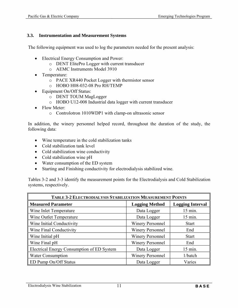
The crystallization process happens in two phases: the induction phase (where precipitates appear in wine due to solubility change caused by chill proofing) and the crystal growth phase. The drastic “slope” change in Figure 4-2 delimits these two phases. Also, Figure 4-2 shows that cold stabilization reduced wine conductivity variation in Tank 953 from 15.5% down to 3.2%. Cold Stabilization Energy Analysis Wine temperature was brought down from approximately 50 ºF to 28 ºF. During the 46 days required to stabilize the wine in Tanks 952 and 953, the refrigeration system (which includes the refrigeration compressor, glycol supply pump, cooling tower fan and cooling tower pump) consumed approximately 26,891 kWh. Figure 4-3 shows the electrical demand for the whole refrigeration system.

0

5

10

15

20

25

30

35

1/23 1/28 2/2 2/7 2/12 2/17 2/22 2/27 3/4 3/9 3/14 3/19 3/24 3/29

Dem

and

(kW

)

Figure 4-3 Refrigeration System Demand

The average demand while dropping the wine temperature from 50 ºF to 28 ºF was 25.2 kW. The average demand required to maintain the tank temperature at 28 ºF was approximately 24.2 kW. Based on a thermodynamic model of the cold stabilization system, the total electrical energy consumption can be broken down into the following components5: Cooling wine from 50 ºF to 28 ºF (both tanks) Cooling the wine = 297 kWh Heat gain from tank sides and top = 538 kWh Heat gain from ground = 21 kWh Formulation of ice on tank surface = 873 kWh 5 Calculation details for the thermodynamic model of the cold stabilization system can be found at the end of the report in the Appendix Section.


15


Heat gain due to uninsulated pipes = 25 kWh Maintaining Tank Temperature at 28 ºF (both tanks) Heat gain form tank sides and top = 6,920 kWh Heat gain from ground = 89 kWh Heat gain due to uninsulated pipes = 372 kWh Total electrical energy consumption = 9,135 kWh Comparing the thermodynamic model electrical energy consumption with measured data shows that only 42% of the electrical energy has been accounted for in the model. It is suspected that the remaining balance is due to energy required by the wine chemistry.

4.2. Electrodialysis Measurements and Analysis Electrodialysis Stabilization and Energy Analysis Electrodialysis stabilization lasted approximately 1.5 days, from January 23, 2007 (9:40 a.m.) through January 24, 2007 (4:11 p.m.). During this period, 21,500 gallons of wine were stabilized by reducing the conductivity change from 14.6% to 2.5%. Figure 4-4 shows the electrodialysis system demand (which includes pumps and membrane electric field generator). The total electrical energy consumption for the electrodialysis system was approximately 165 kWh.

0

1

2

3

4

5

6

7

8

1/23

/07

0:00

1/23

/07

2:00

1/23

/07

4:00

1/23

/07

6:00

1/23

/07

8:00

1/23

/07

10:0

0

1/23

/07

12:0

0

1/23

/07

14:0

0

1/23

/07

16:0

0

1/23

/07

18:0

0

1/23

/07

20:0

0

1/23

/07

22:0

0

1/24

/07

0:00

1/24

/07

2:00

1/24

/07

4:00

1/24

/07

6:00

1/24

/07

8:00

1/24

/07

10:0

0

1/24

/07

12:0

0

1/24

/07

14:0

0

1/24

/07

16:0

0

1/24

/07

18:0

0

1/24

/07

20:0

0

1/24

/07

22:0

0

1/25

/07

0:00

Dem

and

(kW

)

Figure 4-4 Electrodialysis System Demand


16


The average electrical demand for the electrodialysis system is approximately 5 kW. Based on specifications from the electrodialysis manufacturer, the equipment can process wine for approximately 12 hours before it requires CIP (clean-in-place), which typically lasts 1.5 hours. The cleaning cycles are clearly identified in Figure 4-4. Electrodialysis Water Consumption The electrodialysis system requires hard, soft and hot water to operate. Water is mostly used to move the brine solution after dialysis takes place and to perform CIP (clean-in-place) after each 12 hour cycle, or at the end of the batch. The winery personnel recorded the water consumption used by the electrodialysis system for the period of December 18, 2006 through February 15, 2007. For the batch considered in this study, the total water consumption was 6,664 gallons, which is approximately 31% of the total wine volume processed. However, the water consumption for this particular batch was unusually high. To more accurately analyze the water consumption of the electrodialysis system, we will consider the total water consumption processed from December 18, 2006 through February 15, 2007. The total water consumption was approximately 69,948 gallons which represents approximately 14% (504,611 gallons) of the total volume of wine processed through the electrodialysis system for the same period. When considering the economics of an electrodialysis system versus traditional cold stabilization it is important to note that the winery will consume more water (equivalent to 14% of the amount of wine processed through the electrodialysis system). Additionally, if the winery has no waste water ponds, then the wastewater will need to be treated, thus it is necessary to consider the extra energy used for wastewater treatment.

4.3. Limitations on Energy and Demand Savings The baseline considered in this study does not include stabilization tank insulation or stabilization enhancements like wine seeding, mixing, etc. However, to more accurately portray the common practices used in Northern California Wineries, we have adjusted the electrical energy consumption of the cold stabilization system by considering tank insulation on the tank sides. Additionally, recognizing that the new electrodialysis system will result in added water usage and wastewater due to the process, we have included the extra energy that will be required to process the wastewater before discharging it out of the facility.

4.4. Summary of Energy and Demand Savings There may be significant electrical energy and demand savings for stabilizing wine with an electrodialysis system as opposed to traditional cold stabilization. Table 4-1 compares the electrodialysis wine stabilization performance to wine cold stabilization.


17


From Table 4-1, electrodialysis stabilization would result in an overall system energy intensity of 7.9 Wh/gal and cold stabilization would result in an overall system energy intensity of 1,200 Wh/gal. It is expected that electrodialysis stabilization could save approximately 99% of the energy used by traditional cold stabilization.

TABLE 4-1 COLD VS ELECTRODIALYSIS WINE STABILIZATION Stabilization Method Cold Stabilization Electrodialysis Stabilization Energy Consumption 26,891 kWh 165 kWh Average Demand 24 kW 5 kW Increase in Water Consumption 0 gallons 3,010 gallons Adjusted Energy Consumption* 22,965 kWh 170 kWh Stabilization Period 1,108 hours 31 hours Initial Conductivity Drop 14.8% 14.6% Final Conductivity Drop 3.4% 2.5% Volume of Stabilized Wine 18,500 gallons 21,500 gallons Energy Intensity 1,200 Wh/gal 7.9 Wh/gal

* The adjusted cold stabilization energy consumption considers the added tank and bare pipe insulation. The adjusted electrodialysis stabilization energy consumption considers the extra energy needed for wastewater treatment.


18


5. CONCLUSIONS Application of Electrodialysis Stabilization Technology Based on a brief discussion with the winery personnel, the winery was extremely satisfied with the performance of the electrodialysis system. The facility did not notice any adverse effect on the quality of wine produced. Additionally, the winery was very happy with the reduction in stabilization time that was observed when compared to traditional cold stabilization. Besides the increased water consumption and potential wastewater treatment that may be necessary, the electrodialysis stabilization technology may be considered as a suitable alternative to cold stabilization. Energy and Demand Savings due to Application of Electrodialysis Technology Using electrodialysis wine stabilization as opposed to traditional cold stabilization, in the absence of any enhancements, may result in significant electrical energy and demand savings. Based on the study performed, for a small system that cold stabilizes approximately 20,000 gallons of wine, it is expected that application of electrodialysis stabilization could result in approximately 23,842 kWh savings when compared to cold stabilization and reduce the average electrical demand by 19 kW. These results may vary depending on the type of wine, chilling system and the cold stabilization method. Other Associated Issues Because only 42% of the electrical energy consumption of the refrigeration system was accounted for in the thermal model, a full energy balance of the system would require a more detailed analysis of the wine chemistry for the crystallization process. It is important to note that electrodialysis may increase water consumption at the facility (by approximately 14% of the total volume of wine that is processed trough electrodialysis) resulting in additional wastewater. The added wastewater will need to be treated, which may increase the initial capital cost of an electrodialysis system (to include the wastewater treatment equipment).


19


6. APPENDIX

6.1. Thermodynamic Model for Cold Stabilization The thermodynamic analysis for cold stabilization includes the following:

Estimate of electrical energy required for initially cooling the wine to the desired (steady state) temperature.

Estimate of electrical energy required by the refrigeration system to compensate for the heat gain to the wine tank (from the sides, top and bottom of tank) from warmer ambient conditions.

Estimate of electrical energy required to form the layer of ice (which acts as a layer of insulation) on the tank wall surface, since the tank is not insulated.

Estimate of electrical energy required by refrigeration system to compensate for the heat gain to the uninsulated portions of the glycol supply and bypass pipelines.

Estimate the cooling load provided by the glycol based on measured data. Section 6.3 shows the equations that were used in our thermodynamic analysis of the system and Section 6.4 shows a sample of the calculations performed for Tank 952. A summary of the thermodynamic analysis yields the results presented in Table 6-1 below.

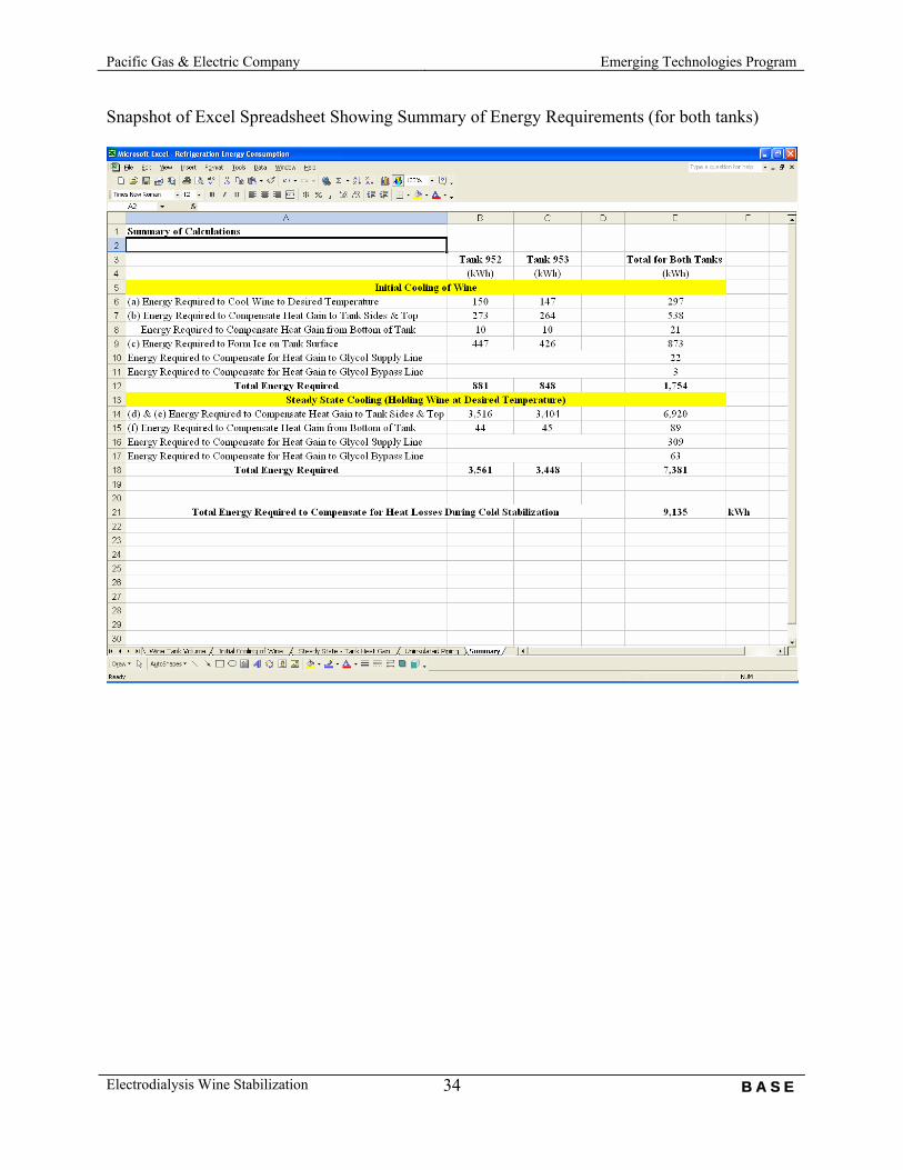
TABLE 6-1 RESULTS OF THERMODYNAMIC ANALYSES Tank 952 Tank 953 Both Tanks

(kWh) (kWh) (kWh) Initial Cooling of Wine to Desired Temperature

Energy Required to Cool Wine to Desired Temperature 150 147 297 Energy Required to Compensate for Heat Gain to Tank Sides and Top of Tank 273 264 538

Energy Required to Compensate for Heat Gain from Bottom of Tank 10 10 21

Energy Required to Form Ice on Tank Surface 447 426 873 Energy Required to Compensate for Heat Gain to Uninsulated Glycol Pipelines 25 25

Total Energy Required During Initial Cooling of Wine 1,754 kWh Steady State Cooling (Holding Wine at Desired Temperature)

Energy Required to Compensate for Heat Gain to Tank Sides and Top of Tank 3,516 3,404 6,920

Energy Required to Compensate for Heat Gain from Bottom of Tank 44 45 89

Energy Required to Compensate for Heat Gain to Uninsulated Glycol Pipelines 372 372

Total Energy Required During Steady State Cooling of Wine 7,381 kWh

Total Energy Required to Compensate for Heat Gain During Cold Stabilization 9,135 kWh


20


From Table 6-1, it can be seen that the total energy required by the refrigeration system during the cold stabilization process is estimated to be 9,135 kWh based on our thermodynamic model. This compares to the measured energy consumption of 26,891 kWh from logged data. A separate analysis of the cooling load provided by the glycol was performed for comparison with the two above methods. Based on measured data for the following parameters:

Glycol supply temperature Glycol tank temperature Glycol bypass flowrate Nominal glycol pump flow (from pump nameplate data)

the electrical energy required by the refrigeration system to provide the necessary glycol cooling was calculated to be 24,322 kWh. A comparison of the 3 sets of data shows that the glycol cooling analysis compares fairly closely with the logged data, with a difference of less than 8%. However, there is a huge discrepancy between the thermodynamic analyses of the heat gain to the wine tank in comparison with the other two values. This can be contributed, but not limited, to the following issues:

Energy required for crystallization Glycol leak, which happened towards the end of cold stabilization.

6.2. Project Timeline and Key Dates Originally the project was scheduled to last two months; the first month allocated to collect data and the second month for analysis and reporting. However, the refrigeration system used for cold stabilization had two major shutdowns due to failure of cooling tower basin level sensor and a minor glycol leak. Due to these two events, cold stabilization did not end until the end of April 2007. Table 6-2 outlines the project timeline and identifies key dates throughout the study.

TABLE 6-2 PROJECT TIMELINE AND KEY DATES Event Dec. 2006 Jan. 2007 Feb. 2007 Mar. 2007 Apr. 2007 May. 2007Kickoff Meeting Monitoring Planning ED Monitoring Cold Stab. Monit. Data Analysis Report Development Refrigeration System Failure First Draft Due Report Due Date


21


6.3. Equations Used for Thermodynamic Model Analysis This section presents the equations that were used in our thermodynamic model to estimate the energy required by the facility’s refrigeration system to compensate for the various sources of heat losses. Volume of Tank

HTank

DTank

x

The volume of wine in a tank can be calculated as follows: V = (ΠDTank

2/4) × (HTank – x) Where, DTank = diameter of tank, feet HTank = height of tank, feet x = distance from top of tank to the level of wine, feet The surface area of the sides of the tank that is covered in ice is estimated as: Aside = (ΠDTank) × (HTank – x) Since the tank is not completely filled with wine, the heat transfer from the sides of the tank (up to the wine level) will be different than the heat transfer from the top of the tank. It should also be noted that 50% of the tank is jacketed for glycol circulation (see Figure 3-3) and the rest of the tank is not jacketed.


22


Equations for Analysis of Energy Used for Cold Stabilization a - Amount of Energy to Cool Wine to Desired Temperature The amount of electrical energy required to cool a given volume of wine, ERCooling, can be estimated as follows: ERCooling = V × ρ × CP × (Tinitial – Tfinal) / (COP × C4) Where, V = volume of wine being cooled, gallons ρ = density of wine, lbm/gallon CP = specific heat of wine, Btu/lbm-°F Tinitial = initial temperature of wine, °F Tfinal = final (or desired) temperature of wine, °F C4 = Conversion factor, 3,412.2 Btu/kW-hr COP = coefficient of performance of refrigeration system b - Energy Required for Tank to Come to Stabilization Temperature (Initial Cooling) (Taken at Average Point Before Wine Has Reached Steady State Temperature) (i) Convective Heat Transfer Coefficient (ASHRAE Fundamentals Eq. 24-6) The convective heat transfer coefficient, hcv,i, is calculated6 as hcv,i = C × (1/d)0.2 × (1/Tavg,i)0.181 × (Tamb,i - Ts,i)0.266 × [1 + 1.277(vwind)]0.5

where, C = constant depending on shape and heat flow condition,

(1.235 for longer vertical cylinders; 0.89 for horizontal plates, cooler than air facing upward)

d = for flat surfaces and large cylinders, d = 24 inches Tavg,i = average temperature (Tavg = (Tamb + Ts) / 2), °F Tamb,i = average ambient air temperature during initial cooling period (from measured data), °F Ts,i = average tank surface temperature during initial cooling (prior to achieving steady state temperature), °F vwind = average air speed, mph

6 Detailed formulation of the heat transfer coefficient had also been compared to formulations from the following references and the results were very comparable:

1) Fundamentals of Heat and Mass Transfer, Frank Incropera & David De Witt, John Wiley & Sons, 1981.

2) Heat Transfer, J. P. Holman, McGraw-Hill Publishing Company, 1990.


23


(ii) Radiative Heat Transfer Coefficient (ASHRAE Fundamentals Eq. 24-7) The radiation heat transfer coefficient, hrad,i, is calculated as: hrad,i = [ε × σ × (Tamb,i

4 – Ts,i4)] / (Tamb,i – Ts,i)

where, ε = surface emittance σ = Stefan-Boltzmann constant, 0.1713 × 10-8 Btu/hr-ft2-R4 The total heat transfer coefficient, hi, is the sum of the convective and radiative heat transfer coefficients: hi = hcv,i + hrad,i (iii) Heat Gain to Tank Surfaces Tank Sides The heat gain (energy) rate, HGside,i, from the sides of the tank surface during the initial cooling period can be estimated as follows:

kk

k

ksidei

iwineiambiside

Akx

Ah

TTHG

tantan

tan

tan,

,,, 1 Δ

+

−=

Where, Tamb,i = average ambient air temperature during initial cooling period (from measured data), °F Twine,i = average wine temperature during initial cooling (prior to achieving steady state temperature), °F hi,side = the sum of the convective heat and radiation heat transfer coefficients for tank sides7, Btu/hr-ft2-°F Atank = area of sides of tank, ft2

∆xtank = thickness of tank wall, feet ktank = thermal conductivity of tank wall material, Btu/hr-ft-°F

7 Calculated from equations (6) and (7) on pages 24.16 and 24.17, Chapter 24 of ASHRAE 1997 Fundamentals


24


Top of Tank The heat gain (energy) rate, HGtop,i, from the top of the tank during the initial cooling period can be estimated as follows:

kk

k

topair

iair

toptopi

iwineiambitop

Akx

Akx

Ah

TTHG

tantan

tan,

,

,,, 1 Δ

+Δ

+

−=

Where, hi,top = the sum of the convective heat and radiation heat transfer coefficients for top of tank, Atop = area of top of tank, ft2

∆xair,i = thickness of layer of air between top surface of wine and tank during initial cooling period, feet kair = thermal conductivity of air, Btu/hr-ft-°F

The term (kk

k

Akx

tantan

tanΔ ) was calculated and was insignificant compared with the other two terms

and have thus not been included in the sample calculations shown in Section 6.3. (iv) Energy to Compensate for Heat Gain to Tank Sides and Top of Tank (Initial Cooling) The amount of electrical energy (kWh) required to compensate for the heat gain from the sides of the tank during the initial cooling period, ERside,i, can be estimated as follows: ERside,i = (HGside,i + HGtop,i)× Hi / (COP × C4) Where, HGside,i = heat gain rate to the tank from tank sides prior to wine achieving steady

state temperature, Btu/hr Hi = hours that tank of wine is initially cooled prior to reaching steady state

temperature, hr COP = coefficient of performance of refrigeration system (calculated based on

measured data) C4 = conversion constant, 3,412.2 Btu/kW-hr


25


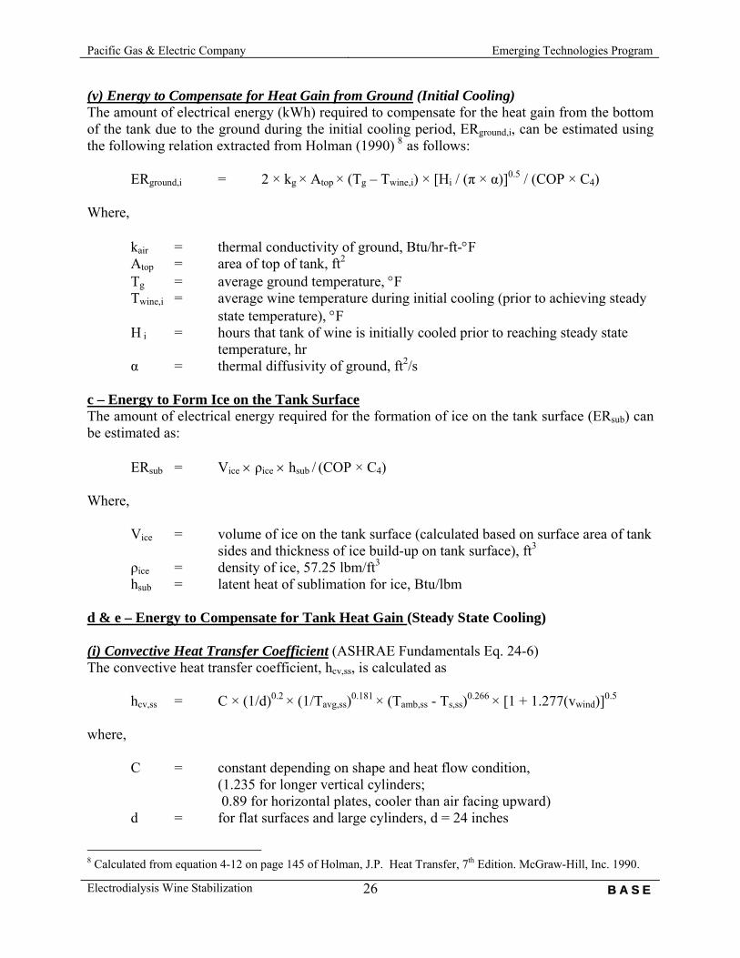
(v) Energy to Compensate for Heat Gain from Ground (Initial Cooling) The amount of electrical energy (kWh) required to compensate for the heat gain from the bottom of the tank due to the ground during the initial cooling period, ERground,i, can be estimated using the following relation extracted from Holman (1990) 8 as follows: ERground,i = 2 × kg × Atop × (Tg – Twine,i) × [Hi / (π × α)]0.5 / (COP × C4) Where, kair = thermal conductivity of ground, Btu/hr-ft-°F Atop = area of top of tank, ft2

Tg = average ground temperature, °F Twine,i = average wine temperature during initial cooling (prior to achieving steady state temperature), °F H i = hours that tank of wine is initially cooled prior to reaching steady state

temperature, hr α = thermal diffusivity of ground, ft2/s c – Energy to Form Ice on the Tank Surface The amount of electrical energy required for the formation of ice on the tank surface (ERsub) can be estimated as: ERsub = Vice × ρice × hsub / (COP × C4) Where,

Vice = volume of ice on the tank surface (calculated based on surface area of tank sides and thickness of ice build-up on tank surface), ft3

ρice = density of ice, 57.25 lbm/ft3 hsub = latent heat of sublimation for ice, Btu/lbm d & e – Energy to Compensate for Tank Heat Gain (Steady State Cooling) (i) Convective Heat Transfer Coefficient (ASHRAE Fundamentals Eq. 24-6) The convective heat transfer coefficient, hcv,ss, is calculated as hcv,ss = C × (1/d)0.2 × (1/Tavg,ss)0.181 × (Tamb,ss - Ts,ss)0.266 × [1 + 1.277(vwind)]0.5


(1.235 for longer vertical cylinders; 0.89 for horizontal plates, cooler than air facing upward)

d = for flat surfaces and large cylinders, d = 24 inches

8 Calculated from equation 4-12 on page 145 of Holman, J.P. Heat Transfer, 7th Edition. McGraw-Hill, Inc. 1990.


26


Tavg,ss = average temperature (Tavg = (Tamb + Ts) / 2), °F Tamb,ss = average ambient air temperature during steady state period (from measured data), °F Ts,ss = average tank surface temperature during steady state period, °F vwind = average air speed, mph (ii) Radiative Heat Transfer Coefficient (ASHRAE Fundamentals Eq. 24-7) The radiation heat transfer coefficient, hrad,ss, is calculated as: hrad,ss = [ε × σ × (Tamb,i

4 – Ts,i4)] / (Tamb,ss – Ts,ss)

where, ε = surface emittance σ = Stefan-Boltzmann constant, 0.1713 × 10-8 Btu/hr-ft2-R4 The total heat transfer coefficient, hi, is the sum of the convective and radiative heat transfer coefficients: hss = hcv,ss + hrad,ss (iii) Heat Gain from Tank Surfaces Tank Sides The heat gain (energy) rate, HGside,ss, from the sides of the tank surface during the steady state (holding) period can be estimated as follows:

sideice

ice

sidek

k

sidesidess

sswinessambssside

Akx

Akx

Ah

TTHG

Δ+

Δ+

−=

tan

tan

,

,,, 1

Where, Tamb,i = average ambient air temperature during steady state cooling period, °F Twine,i = average wine temperature during steady state cooling, °F hss,side = the sum of the convective heat and radiation heat transfer coefficients for tank sides9, Btu/hr-ft2-°F Aside = area of sides of tank, ft2

∆xtank = thickness of tank wall, feet ktank = thermal conductivity of tank wall material, Btu/hr-ft-°F ∆xice = thickness of ice build-up on tank wall, feet kice = thermal conductivity of ice, Btu/hr-ft-°F

9 Calculated from equations (6) and (7) on pages 24.16 and 24.17, Chapter 24 of ASHRAE 1997 Fundamentals


27


Top of Tank The heat gain (energy) rate, HGtop,ss, from the top of the tank during the steady state (holding) period can be estimated as follows:

sidek

k

topair

ssair

toptopss

sswinessambstop

Akx

Akx

Ah

TTHG

tan

tan,

,

,,, 1 Δ

+Δ

+

−=

Where, hi = the sum of the convective heat and radiation heat transfer coefficients for top of tank, Atop = area of top of tank, ft2

∆xair,s = thickness of layer of air between top surface of wine and tank during steady state cooling period, feet kair = thermal conductivity of air, Btu/hr-ft-°F

The term (kk

k

Akx

tantan

tanΔ ) was calculated and found to be insignificant compared with the other two

terms and have thus not been included in the sample calculations shown in Section 6.3. (iv) Energy to Compensate for Heat Gain from Tank Sides and Top of Tank (Steady State Cooling) The amount of electrical energy (kWh) required to compensate for the heat gain from the sides of the tank during the steady state cooling period, ERside,ss, can be estimated as follows: ERside,ss = (HGside,ss + HGtop,ss)× Hss / (COP × C4) Where, HGside,ss = heat gain rate to the tank from tank sides during steady state period, Btu/hr Hss = hours that tank of wine is held at steady state temperature, hr COP = coefficient of performance of refrigeration system (calculated based on



28


f – Energy to Compensate for Heat Gain from Ground (Steady State Cooling) The amount of electrical energy (kWh) required to compensate for the heat gain from the bottom of the tank due to the ground during the steady state period, ERground,ss, can be estimated as follows: ERground,ss = 2 × kg × Atop × (Tg – Twine,ss) × [Hss / (π × α)]0.5 / (COP × C4) Where, kair = thermal conductivity of ground, Btu/hr-ft-°F Atop = area of top of tank, ft2

Tg = average ground temperature, °F Twine,ss = average wine temperature during steady state cooling period, °F Hss = hours that tank of wine is held at steady state temperature, hr α = thermal diffusivity of ground, ft2/s g – Energy to Compensate for Heat Gain Due to Uninsulated Glycol Piping Convective Heat Transfer Coefficient (ASHRAE Fundamentals Eq. 24-6) The convective heat transfer coefficient, hcv, is calculated as hcv = C × (1/d)0.2 × (1/Tavg)0.181 × (Tamb - Ts)0.266 × [1 + 1.277(vwind)]0.5


(1.016 for horizontal cylinders; 1.235 for longer vertical cylinders)

d = diameter for cylinder, inches Tavg = average temperature (Tavg = (Tamb + Ts) / 2), °F Tamb = average ambient air temperature, °F Ts = average surface temperature, °F vwind = average wind speed, mph Radiative Heat Transfer Coefficient (ASHRAE Fundamentals Eq. 24-7) The radiation heat transfer coefficient, hrad, is calculated as: hrad = [ε × σ × (Tamb

4 – Ts4)] / (Tamb – Ts)

where, ε = surface emittance σ = Stefan-Boltzmann constant, 0.1713 × 10-8 Btu/hr-ft2-R4


29


The total heat transfer coefficient, hi, is the sum of the convective and radiative heat transfer coefficients: hpipe = hcv + hrad Heat Gain from Uninsulated Glycol Pipelines The heat gain by the uninsulated piping due to the outside ambient temperature, HGpipe, can be estimated as follows:

pipeice

ice

pipepipe

pipe

pipepipe

glycolambpipe

Akx

Akx

Ah

TTHG

Δ+

Δ+

−=

1

Where, Tamb = average ambient air temperature, °F Tglycol = average glycol temperature, °F hpipe = the sum of the convective heat and radiation heat transfer coefficients for uninsulated piping, Apipe = area of uninsulated piping, ft2

∆xtank = thickness of pipe wall, feet ktank = thermal conductivity of piping material, Btu/hr-ft-°F ∆xice = thickness of ice build-up on piping, feet kice = thermal conductivity of ice, Btu/hr-ft-°F Energy to Compensate for Heat Gain by Uninsulated Glycol Piping The amount of electrical energy (kWh) required to compensate for the heat gain from the uninsulated glycol pipelines, ERpipe, can be estimated as follows: ERpipe = HGpipe× Hcs / (COP × C4) Where, HGpipe = heat gain rate to the uninsulated glycol pipelines, Btu/hr Hss = total hours required for cold stabilization process, hr COP = coefficient of performance of refrigeration system (calculated based on



30


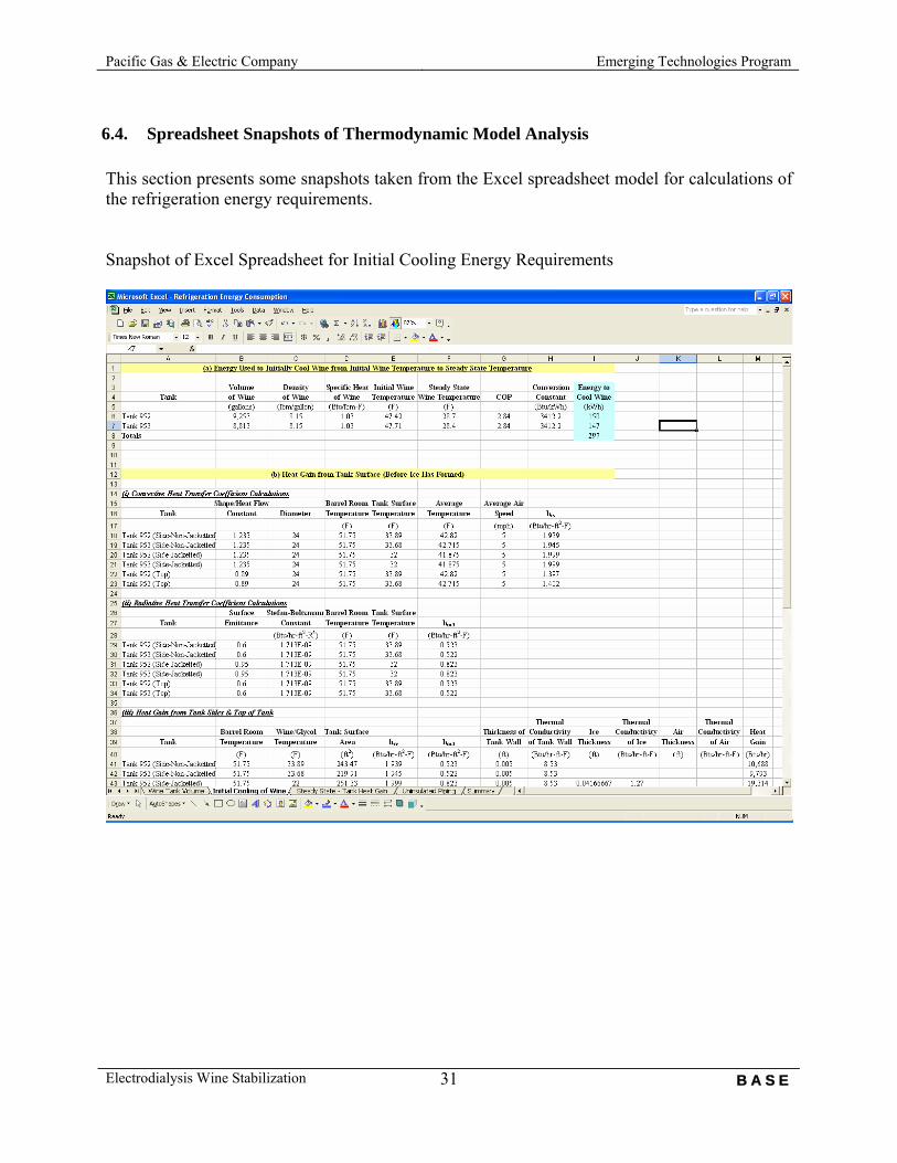
6.4. Spreadsheet Snapshots of Thermodynamic Model Analysis This section presents some snapshots taken from the Excel spreadsheet model for calculations of the refrigeration energy requirements. Snapshot of Excel Spreadsheet for Initial Cooling Energy Requirements


31


Snapshot of Excel Spreadsheet for Steady State Cooling Energy Requirements


32


Snapshot of Excel Spreadsheet for Uninsulated Piping Energy Requirements


33


Snapshot of Excel Spreadsheet Showing Summary of Energy Requirements (for both tanks)


34



35

6.5. Graphs of Data Recorded During Cold Stabilization and Electrodialysis Tests This section presents some graphs of the various measurements that were recorded throughout the cold stabilization and electrodialysis tests.

0

20

40

60

80

100

120

1/18 1/23 1/28 2/2 2/7 2/12 2/17 2/22 2/27 3/4 3/9 3/14 3/19 3/24 3/29 4/3 4/8 4/13 4/18 4/23 4/28

Tem

pera

ture

(F)

Outdoor Temperature Barrel Room ED Trailer

Figure 6.5-1 Ambient Temperatures

0

10

20

30

40

50

60

70

1/18 1/23 1/28 2/2 2/7 2/12 2/17 2/22 2/27 3/4 3/9 3/14 3/19 3/24 3/29 4/3 4/8 4/13 4/18 4/23 4/28

Tem

pera

ture

(F)

Tank 952 - Surface Tank 952 - Well Tank 953 - Surface

Tank 953 - Well Glycol Return Glycol Supply

Figure 6.5-2 Cold Stabilization Tank Temperatures


0

10

20

30

40

50

60

70

80

90

1/18 1/20 1/22 1/24 1/26 1/28 1/30 2/1 2/3 2/5 2/7 2/9 2/11 2/13

Tem

pera

ture

(F)

ED Wine In ED Wine Out

Figure 6.5-3 Electrodialysis Test Wine Temperature

0

5

10

15

20

25

30

35

40

1/18 1/23 1/28 2/2 2/7 2/12 2/17 2/22 2/27 3/4 3/9 3/14 3/19 3/24 3/29 4/3 4/8 4/13 4/18 4/23 4/28

Dem

and

(kW

)

Cold Stabilization ED Stabilization

Figure 6.5-4 Measured Electrical Demand for Cold Stabilization vs. Electrodialysis Tests


36


0

5,000

10,000

15,000

20,000

25,000

30,000

35,000

40,000

45,000

50,000

1/18 1/23 1/28 2/2 2/7 2/12 2/17 2/22 2/27 3/4 3/9 3/14 3/19 3/24 3/29 4/3 4/8 4/13 4/18 4/23 4/28

Con

sum

ptio

n (k

Wh)

Cold Stabilization ED Stabilization

Figure 6.5-5 Measured Electrical Energy Consumption for Cold Stabilization vs. Electrodialysis Tests

0.0%

2.0%

4.0%

6.0%

8.0%

10.0%

12.0%

14.0%

16.0%

18.0%

1/18 1/22 1/26 1/30 2/3 2/7 2/11 2/15 2/19 2/23 2/27 3/3 3/7 3/11 3/15 3/19 3/23 3/27 3/31 4/4

Con

duct

ivity

(%)

Tank 952 Tank 953

Figure 6.5-6 Cold Stabilization Wine Conductivity Tests for Both Tanks


37

Documents

Pacific Gas and Electric Company - BASE Energy, Inc. Report - Wine Stabilization... · Pacific Gas and Electric Company Emerging Technologies Program Application Assessment Report