Measuring Business Cycles: A Modern Perspective

Francis X. Diebold

University of Pennsylvania

Glenn D. Rudebusch

Federal Reserve Bank of San Francisco

This Print: June 27, 1996

Abstract: In the first half of this century, special attention was given to two features of the

business cycle: the comovement of many individual economic series and the different

behavior of the economy during expansions and contractions. Recent theoretical and

empirical research has revived interest in each attribute separately, and we survey this work.

Notable empirical contributions are dynamic factor models that have a single common

macroeconomic factor and nonlinear regime-switching models of a macroeconomic

aggregate. We conduct an empirical synthesis that incorporates both of these features.

JEL Classification Codes: E32, C22

Diebold, F.X. and Rudebusch, G. (1996), "Measuring Business Cycles: A Modern Perspective,"

Review of Economics and Statistics, 78, 67-77.

1

I. Introduction

It is desirable to know the facts before attempting to explain them; hence, the

attractiveness of organizing business-cycle regularities within a model-free framework.

During the first half of this century, much research was devoted to obtaining just such an

empirical characterization of the business cycle. The most prominent example of this work

was Burns and Mitchell (1946), whose summary empirical definition was:

Business cycles are a type of fluctuation found in the aggregate economic activity of

nations that organize their work mainly in business enterprises: a cycle consists of

expansions occurring at about the same time in many economic activities, followed by

similarly general recessions, contractions, and revivals which merge into the expansion

phase of the next cycle. (p. 3)

Burns and Mitchell's definition of business cycles has two key features. The first is the

comovement among individual economic variables. Indeed, the comovement among series,

taking into account possible leads and lags in timing, was the centerpiece of Burns and

Mitchell's methodology. In their analysis, Burns and Mitchell considered the historical

concordance of hundreds of series, including those measuring commodity output, income,

prices, interest rates, banking transactions, and transportation services. They used the clusters

of turning points in these individual series to determine the monthly dates of the turning

points in the overall business cycle. Similarly, the early emphasis on the consistent pattern of1

comovement among various variables over the business cycle led directly to the creation of

composite leading, coincident, and lagging indexes (e.g., Shishkin, 1961).

The second prominent element of Burns and Mitchell's definition of business cycles is

their division of business cycles into separate phases or regimes. Their analysis, as was

typical at the time, treats expansions separately from contractions. For example, certain series

are classified as leading or lagging indicators of the cycle, depending on the general state of

business conditions.

2

Both of the features highlighted by Burns and Mitchell as key attributes of business

cycles were less emphasized in postwar business-cycle models--particularly in empirical

models where the focus was on the time-series properties of the cycle. Most subsequent

econometric work on business cycles followed Tinbergen (1939) in using the linear difference

equation as the instrument of analysis. This empirical work has generally focused on the

time-series properties of just one or a few macroeconomic aggregates, ignoring the pervasive

comovement stressed by Burns and Mitchell. Likewise, the linear structure imposed

eliminated consideration of any nonlinearity of business cycles that would require separate

analyses of expansions and contractions.

Recently, however, empirical research has revived consideration of each of the

attributes highlighted by Burns and Mitchell. Notably, Stock and Watson (1989, 1991, 1993)

have used a dynamic factor model to capture comovement by obtaining a single common

factor from a set of many macroeconomic series, and Hamilton (1989) has estimated a

nonlinear model for real GNP with discrete regime switching between periods of expansion

and contraction.

This paper is part survey, part interpretation, and part new contribution. We describe

the dynamic-factor and regime-switching models in some detail in sections II and III, and we

sketch their links to recent developments in macroeconomics in section IV. The modern

dynamic-factor and regime-switching literatures, however, have generally considered the

comovement and regime-switching aspects of the business cycle in isolation of each other.

We view that as unfortunate, as scholars of the cycle have simultaneously used both ideas for

many decades. Thus, in section V, we attempt an empirical synthesis in a comprehensive

framework that incorporates both factor structure and regime switching. We conclude in

section VI.

3

II. Comovement: Factor Structure

In a famous essay, Lucas (1976) drew attention to a key business-cycle fact: outputs

of broadly-defined sectors move together. Lucas' view is part of a long tradition that has

stressed the coordination of activity among various economic actors and the resulting

comovement in sectoral outputs.

Analysis of comovement in dynamic settings typically makes use of two

nonparametric tools, the autocorrelation function and the spectral density function. In the

time domain, one examines multivariate dynamics via the autocorrelation function, which

gives the correlations of each variable with its own past and with the past of all other variables

in the system. Such analyses are now done routinely, as in Backus and Kehoe (1992), who

characterize the dynamics of output, consumption, investment, government purchases, net

exports, money, and prices across ten countries and a hundred years.

Alternatively, one examines dynamics in the frequency domain via the spectral density

function, the Fourier transform of the autocovariance function, which presents the same

dynamic information but in a complementary fashion. The spectral density matrix

decomposes variation and covariation among variables by frequency, permitting one to

concentrate on the dynamics of interest (business-cycle dynamics, for example, correspond to

periods of roughly 2-8 years). Transformations of both the real and imaginary parts of the

spectral density matrix have immediate interpretation in business-cycle analysis; the

coherence between any two economic time series effectively charts the strength of their

correlation by frequency, while the phase charts lead/lag relationships by frequency. A good

example of business-cycle analysis in the frequency domain is Sargent (1987), who examines

the spectral density matrix of seven U.S. data series: real GNP, the unemployment rate, the

interest rate, the change in real money stock, inflation, productivity, and real wages. 2

Of course, one can analyze business-cycle data parametrically as well, by

approximating the dynamic relationships with a particular statistical model. In this regard, the

4

vector autoregression, introduced by Sims (1980), is ubiquitous. The moving-average

representation (that is, the impulse-response function) of a vector autoregression of a set of

macroeconomic variables provides a readily-interpretable characterization of dynamics, by

charting the response of each variable to shocks to itself and the other variables.

Unfortunately, a vector-autoregressive study that attempts to capture the pervasive

comovement among hundreds of series emphasized by Burns and Mitchell requires more

degrees of freedom than are available in macroeconomic samples. Recent work provides

crucial dimensionality reduction, however, because the dynamic comovements among large

sets of macroeconomic variables are often well-described by a particular configuration of the

vector autoregression associated with index structure, or factor structure.

Factor models have a long history of use in cross-sectional settings, and their

generalization to dynamic environments is due to Sargent and Sims (1977), Geweke (1977)

and Watson and Engle (1983). Important recent contributions include Stock and Watson

(1989, 1991, 1993) and Quah and Sargent (1993), among others. The idea is simply that the

comovement of contemporaneous economic variables may be due to the fact that they are

driven in part by common shocks. In a one-factor model, for example, the behavior of the set

of N variables is qualitatively similar to the behavior of just one variable, the common factor.

This allows parsimonious modeling while nevertheless maintaining fidelity to the notion of

pervasive macroeconomic comovement. 3

Let us focus on the dynamic factor model of Stock and Watson (1991), which was

developed as a modern statistical framework for computing a composite index of coincident

indicators. In their one-factor model, movements in the N macroeconomic variables of

interest, x , are determined by changes in the one-dimensional unobserved common factor, f ,t t

and by the N-dimensional idiosyncratic component, u :t

xt ft utNx1 Nx1 Nx1 1x1 Nx1

D(L) ut tNxN Nx1 Nx1

(L)(ft ) t .1x1 1x1 1x1

t,

t.

{u1t, ..., uNt, ft}

{ 1t, ..., Nt, t} var( t) 1.

5

All idiosyncratic stochastic dynamics are driven by while all common stochastic

dynamics, which are embodied in the common factor, are driven by Identification may

be achieved in many ways. Stock and Watson, for example, impose (1) orthogonality at all

leads and lags of (which is achieved by making D(L) diagonal and

orthogonal at all leads and lags), and (2)

III. Nonlinearity: Regime Switching

Underlying much of the traditional business-cycle literature is the notion that a good

statistical characterization of business-cycle dynamics may require some notion of regime

switching between "good" and "bad" states. Models incorporating regime switching have a4

long tradition in dynamic econometrics. One recent time-series model squarely in line with5

the regime-switching tradition is the "threshold" model (e.g., Tong, 1983; Potter, 1995). In a

threshold model, the regime switches according to the observable past history of the system.

Although threshold models are of interest, models with latent states as opposed to

observed states may be more appropriate for business-cycle modeling. Hamilton (1989, 1990,

1994) develops such models. In Hamilton's regime-switching setup, time-series dynamics are

governed by a finite-dimensional parameter vector that switches (potentially each period)

Mp00 1 p00

1 p11 p11

.

f(yt st; ) 12

exp(yt µst

)2

2 2.

{st}Tt 1

{yt}Tt 1

{st}Tt 1

6

depending upon which of two unobservable states is realized, with state transitions governed

by a first-order Markov process.

To make matters concrete, let's take a simple example. Let be the (latent)

sample path of two-state first-order Markov process, taking values 0 or 1, with transition

probability matrix given by6

Let be the sample path of an observed time series that depends on such that

the density of y conditional upon s ist t

Thus, y is Gaussian white noise with a potentially switching mean. The two means aroundt

which y moves are of particular interest and may, for example, correspond to episodes oft

differing growth rates ("expansions" and "contractions").

The central idea of regime switching is simply that expansions and contractions may

be usefully treated as different probabilistic objects. This idea has been an essential part of

the Burns-Mitchell-NBER tradition of business-cycle analysis and is also manifest in the great

interest in the popular press, for example, in identifying and predicting turning points in

economic activity. Yet it is only within a regime-switching framework that the concept of a

turning point has intrinsic meaning. Recent contributions that have emphasized the use of

probabilistic models in the construction and evaluation of turning-point forecasts and

chronologies include Neftci (1984) and Diebold and Rudebusch (1989).

Various seemingly-disparate contributions may be readily interpreted within the

context of the basic switching model. One example is Neftci's (1984) well-known analysis of

Mt

exp(zt 0)

1 exp(zt 0)1

exp(zt 0)

1 exp(zt 0)

1exp(zt 1)

1 exp(zt 1)

exp(zt 1)

1 exp(zt 1)

.

7

business-cycle asymmetry, which amounts to asking whether the transition probability matrix

is symmetric. Another example is Potter's (1995) and Sichel's (1994) evidence for the

existence of a "recovery" regime of very fast growth at the beginning of expansions, which

corresponds to a "third state" in business-cycle dynamics.

Yet another class of examples concerns recent analyses of business-cycle duration

dependence, which amount to asking whether the transition probabilities vary with length-to-

date of the current regime. Diebold and Rudebusch (1990), Diebold, Rudebusch and Sichel

(1993), and Filardo (1994) have found positive duration dependence in postwar U.S.

contractions; that is, the longer a contraction persists, the more likely it is to end soon.

Similar results have been obtained by Durland and McCurdy (1994) using the technology of

semi-Markov processes. Other forms of time-variation in business-cycle transition

probabilities may be important as well. Ghysels (1993, 1994), in particular, argues that

business-cycle transition probabilities vary seasonally and provides formal methods for

analyzing such variation.7

The business-cycle duration dependence literature highlights the fact that economic

considerations may suggest the potential desirability of allowing the transition probabilities to

vary through time. The duration dependence literature focuses on trend and seasonal

variation in transition probabilities, but in certain contexts it may be desirable to allow for

more general time-variation, as in Diebold, Lee and Weinbach (1994) and Filardo (1994),

who let the transition probabilities evolve as logistic functions of exogenous variables, z :t

8

IV. Factor Structure and Regime Switching: Links to Macroeconomic Theory

In this section, as further motivation, we describe some of the links between

macroeconomic theory and factor structure and regime switching. We use convex

equilibrium business-cycle models to motivate the appearance of factor structure and non-

convex models with multiple equilibria to motivate regime switching; however, we hasten to

add that these pairings are by no means exclusive. Moreover, of course, our ultimate interest

lies in models that simultaneously display factor structure and regime-switching behavior,

which as the following discussion suggests, might occur in a variety of ways.

A. Macroeconomic Theory and Factor Structure

The econometric tradition of comovement through factor structure is consistent with a

variety of modern dynamic macroeconomic models. Here we highlight just one--a linear-

quadratic equilibrium model--in order to motivate the appearance of factor structure. We

follow the basic setup of Hansen and Sargent (1993), which although arguably rigid in some

respects, has two very convenient properties. First, the discounted dynamic programming

problem associated with the model may be solved easily and exactly. Second, the equilibria

of such models are precisely linear (that is, precisely a vector autoregression), thereby

bringing theory into close contact with econometrics.

Preferences are quadratic and are defined over consumption of services, s , and workt

effort, l , with preference shocks, b , determining a stochastic bliss point. There are four lineart t

constraints on the utility maximization. The first represents the linear technology: a weighted

average of the output of consumption goods, c , intermediate goods, g , and investment goods,t t

i , equals a linear combination of lagged capital stock, k , and work effort, plus thet t-1

technology shock, d . The second is the law of motion for the capital stock: Capitalt

accumulates through additional net investment. The third is the law of motion for "household

capital," h , which is driven by consumption expenditures. The last specifies that currentt

consumption services depend on both lagged household capital and current consumption.

max 12

Et 0

t (st bt) (st bt) l 2t

1ct 2gt 3it 4kt 1 5lt dt

kt 1kt 1 2it

ht 1ht 1 2ct

st 1ht 1 2ct.

et 1 1et wt 1,

bt Ubet

dt Udet.

9

Formally, the planning problem associated with this model is

subject to the four constraints8

The exogenous uncertainty (e ) in the model evolves according to t+1

where w is zero-mean white noise. The preference and technology shocks (b and d ) aret+1 t t

linear transformations of the e ,t

Importantly for our purposes, note that this framework can potentially describe the

determination of a large set of series. All variables (except l ) can be considered as vectors oft

different goods or services with the parameters interpreted as conformable matrices.

The equilibrium of this economy is a linear stochastic process and can be represented

by a vector autoregression constrained by cross-equation restrictions, with state-space form

t 1 A t Cwt 1

ot G t,

t 1 A t Cwt 1

ot G t vt ,

t

10

where the state vector contains h , k , and e . o can contain any variable that can bet t t t

expressed as a linear function of the state variables. Note that this vector autoregression will

be singular so long as the number of shocks is less than the number of variables in the system.

Fewer shocks than observables is the rule in economic models. The standard setups have just

a few preference and technology shocks driving a comparatively large number of decision

variables, thereby building in singularity. In fact, in the leading case of a single technology

shock and no preference shocks, one shock is responsible for all variation in the choice

variables, resulting in an equilibrium that maps into a special (singular) case of the one-factor

model discussed earlier. In that special case, there are no idiosyncratic shocks (or

equivalently, they have zero variance).

To reconcile the singular equilibrium from the model economy with the clearly non-

singular nature of the data, measurement error is often introduced. The state-space9

representation becomes

where v is a martingale-difference sequence. In single-shock linear-quadratic models witht

measurement error, the equilibria are precisely of the single-factor form, with non-degenerate

idiosyncratic effects.

Feeling constrained by linear technology and quadratic preferences, many authors

have recently focused on models that are not linear-quadratic. The formulation is basically10

the same as in the linear-quadratic case, but the mechanics are more complicated. The

11

discounted dynamic programming problem associated with the recursive competitive

equilibrium can only be solved approximately; however, the decision rules are nevertheless

well-approximated linearly near the steady state. Under regularity conditions, the equilibrium

is a Markov process in the state variables, and if that Markov process converges to an

invariant distribution, then a vector-autoregressive representation exists. Again, the vector

autoregression is only an approximation to the generally nonlinear decision rules, and its

computation can be tedious. However, the availability of a factor structure for modelling this

approximation remains.

B. Macroeconomic Theory and Regime Switching

Regime-switching behavior is also consistent with a variety of macroeconomic

models. Here we focus on models with coordination failures, which produce multiple

equilibria. In what follows, we shall provide a brief overview of this theoretical literature and

its relation to the regime-switching model.

Much has been made of the role of spillovers and strategic complementarities in

macroeconomics (Cooper and John, 1988). "Spillover" simply refers to a situation in which

others' strategies affect one's own payoff. "Strategic complementarity" refers to a situation in

which others' strategies affect one's own optimal strategy. Spillovers and strategic

complementarities arise, for example, in models of optimal search (e.g., Diamond, 1982),

where thick-market externalities ensure that the likelihood of successful search depends on

the intensity of search undertaken by others, which in turn affects one's own optimal search

intensity. In short, search is more desirable when other agents are also searching, because it is

likely to be more productive.

Spillovers and strategic complementarities may have important macroeconomic

effects. For example, the appearance of aggregate increasing returns to scale (e.g., Hall,

1991) may simply be an artifact of the positive externalities associated with high output levels

in the presence of spillovers and strategic complementarities rather than true increasing

12

returns in firms' technologies. Indeed, Caballero and Lyons (1992) find little evidence of

increasing returns at the individual level, yet substantial evidence at the aggregate level,

suggesting the importance of spillovers and strategic complementarities.

Spillovers and strategic complementarities can produce multiple equilibria, the

dynamics of which may be well-approximated by statistical models involving regime

switching. In fact, Cooper and John (1988) stress the existence of multiple equilibria, with11

no coordination mechanism, as a common theme in a variety of seemingly-unrelated models

displaying spillovers and strategic complementarities. Moreover, the equilibria are frequently

Pareto-rankable. Situations arise, for example, in which an economy is in a low-output

equilibrium such that all agents would be better off at higher output levels, but there is no

coordination device to facilitate the change. 12

Recent work has provided some mechanisms for endogenizing switches between

equilibria. One approach involves variations on Keynesian "animal spirits," or self-fulfilling

waves of optimism and pessimism, as formalized by Azariadis (1981) and Cass and Shell

(1983). Notably, Diamond and Fudenberg (1989) demonstrate in a search framework the

existence of rational-expectations sunspot equilibria in which agents' beliefs about cycles are

self-fulfilling. Howit and McAfee (1992) obtain results even more in line with our thesis in a

model in which waves of optimism and pessimism evolve according to a Markov process.

The statistical properties of equilibria from their model are well-characterized by a Markov

regime-switching process.13

Finally, Cooper (1994) proposes a history-dependent selection criterion in an economy

with multiple Nash equilibria corresponding to different levels of productivity. The Cooper

criterion reflects the idea that history may create a focal point: a person's recent experience is

likely to influence her expectations of others' future strategic behavior, resulting in a slow

evolution of conjectures about others' actions. Cooper's analysis highlights the importance of

learning to respond optimally to the strategic actions of others. The Cooper criterion leads to

{st}Tt 1

{ft}Tt 1

{st}Tt 1),

ht (st 1, ..., st p, ft 1, ..., ft p) . ft on ht

13

persistence in the equilibrium selected, with switching occurring as a consequence of large

shocks, phenomena which again may be well-characterized by statistical models involving

regime switching.

Other history-dependent theoretical models have been proposed by Startz (1994) and

Acemoglu and Scott (1993). These include the same "learning-by-doing" dynamic externality

that dives the "new growth theory" models. Again, shocks cause endogenous switching

between high-growth and low-growth states.

V. Synthesis: Regime Switching in a Dynamic Factor Model

We have argued that both comovement through factor structure and nonlinearity

through regime switching are important elements to be considered in an analysis of business

cycles. It is unfortunate, therefore, that the two have recently been considered largely in

isolation from each other. In what follows, we sketch a framework for the analysis of

business-cycle data that incorporates both factor structure and regime switching in a natural

way. This framework, although not formally used before, may be a good approximation to

the one implicitly adopted by many scholars of the cycle.

A. A Prototypical Model

Consider a dynamic factor model in which the factor switches regimes. First consider

a switching model for the factor f ; we work with a slightly richer model than before, allowingt

for p -order autoregressive dynamics. Again let be the sample path of a latentth

Markov process, taking on values 0 and 1, let be the sample path of the factor (which

depends on and collect the relevant history of the factor and state in the

vector The probabilistic dependence of is

summarized by the conditional density,

P(ft ht; ) 12

exp(ft µst

)p

i 1i(ft i µst i

)2

2 2.

xt ft utNx1 Nx1 Nx1 1x1 Nx1

D(L) ut t,NxN Nx1 Nx1

µ0 µ1

14

The latent factor, then, follows a pth-order Gaussian autoregression with potentially changing

mean. The two means around which the factor moves are of particular interest; call

them (slow growth) and (fast growth).

We then assemble the rest of the model around the regime-switching factor. We write

as earlier. In Frischian terms, the model as written has a regime-switching "impulse" with a

stable "propagation mechanism". Many variations on the theme of this basic setup are of

course possible.

B. A Look at the Data

Let us first describe the data. We examine quarterly economic indicators, 1952.I -

1993.I, as described in detail in Table 1. The data include three composite indexes of

coincident indicators, corresponding to three alternative methodologies: Commerce

Department, modified Commerce Department, and Stock-Watson. The component indicators

underlying the Commerce Department and modified Commerce Department indexes are

identical (personal income less transfer payments, index of industrial production,

manufacturing and trade sales, and employees on non-agricultural payrolls); only their

processing differs slightly (see Green and Beckman, 1992). The Stock-Watson index

15

introduces a change in the list of underlying indicators (employees on nonagricultural payrolls

is replaced by hours of employees on nonagricultural payrolls) and processes the underlying

component indicators differently than either the Commerce Department or modified

Commerce Department indexes. We obtained qualitatively similar results from all of the

indexes; thus, we shall focus here on the Commerce Department's modified Composite

Coincident Index. Henceforth, we shall refer to it simply as "the Composite Coincident

Index."

We graph the log of the Composite Coincident Index in Figure 1. It tracks the

business cycle well, with obvious and pronounced drops corresponding to the NBER-

designated recessions of 1958, 1960, 1970, 1974, 1980, 1982 and 1990. We similarly graph

the logs of the four components of the Composite Coincident Index in Figure 2. Their14

behavior closely follows that of the Composite Coincident Index; in particular, there seems to

be commonality among switch times.

We shall not provide maximum-likelihood estimates (or any other estimates) of a

fully-specified dynamic-factor model with regime-switching factor. To do so would be

premature at this point. Instead, we shall sift the data in two simple exercises to provide

suggestive evidence as to whether the data accord with our basic thesis.

First, we work directly with the Composite Coincident Index, which is essentially an

estimate of the common factor underlying aggregate economic activity. We ask whether its15

dynamics are well-approximated by a Markov-switching model. We fit a switching model to

one hundred times the change in the natural logarithm of the Composite Coincident Index,

with one autoregressive lag and a potentially switching mean.

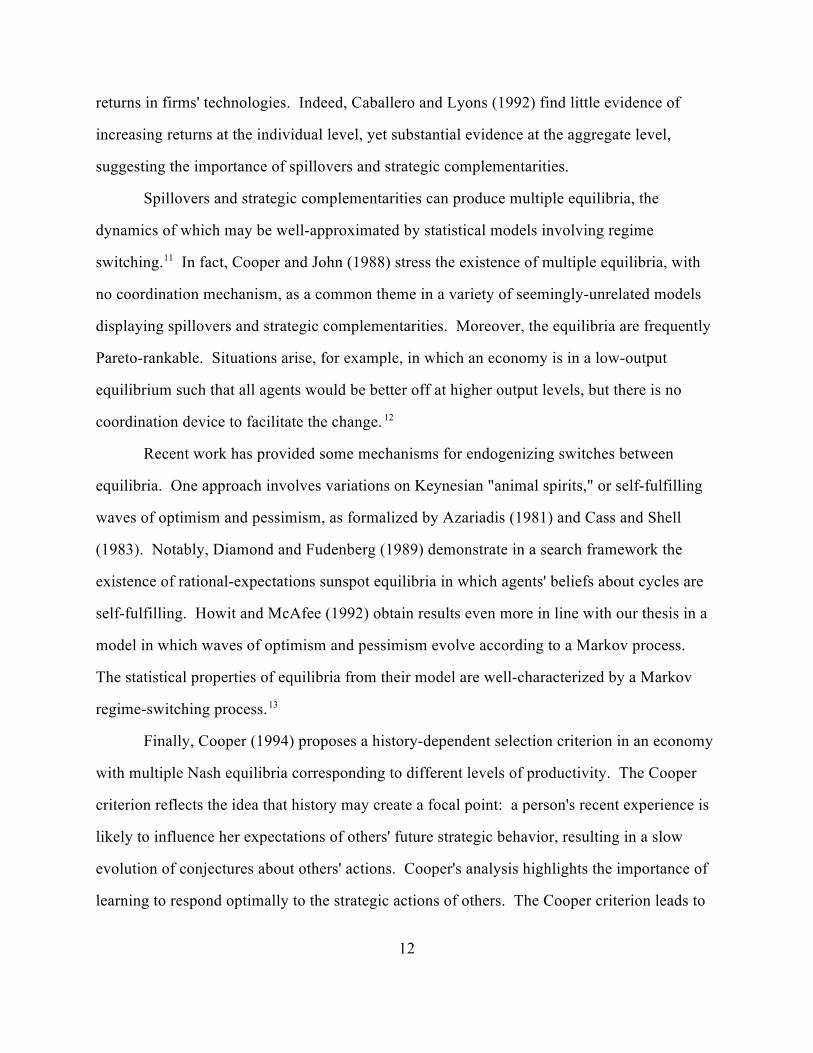
The results appear in the second column of Table 2. Several points are worth16

mentioning. First, the state-0 mean is significantly negative, and the state-1 mean is

significantly positive, and the magnitudes of the estimates are in reasonable accord with our

priors. Second, the within-state dynamics display substantial persistence. Third, the estimates

16

of p and p accord with the well-known fact that expansion durations are longer than00 11

contraction durations on average. Fourth, the smoothed (that is, conditional upon all

observations in the sample) probabilities that the Composite Coincident Index was in state 0

(graphed in Figure 3) are in striking accord with the professional consensus as to the history

of U.S. business cycles.17

In our second exercise, we fit switching models to the individual indicators underlying

the Composite Coincident Index and examine the switch times for commonality. In a similar

fashion to our analysis of the Composite Coincident Index, we fit models to one hundred

times the change in the natural logarithm of each of the underlying coincident indicators, with

one autoregressive lag and potentially switching means.

The results appear in columns three through six of Table 2. The component-by-18

component results are qualitatively similar to those for the Composite Coincident Index, as

would be expected in the presence of a regime-switching common factor. Further evidence in

support of factor structure emerges in Figure 4, in which we graph the time series of

smoothed state-0 probabilities for each of the four component coincident indicators. There is

commonality in switch times, which is indicative of factor structure. Note, however, that the

ability of the individual component indicators to track the business cycle (as captured in the

smoothed state-0 probabilities for each of the component indicators) is inferior to that of the

Composite Coincident Index. This is consistent with the our switching-factor argument.

Individual series are swamped by measurement error and hence provide only very noisy

information on the state of the business cycle, but moving to a multivariate framework

enables more precise tracking of the cycle.

C. Assessing Statistical Significance

Thus far, our empirical work has proceeded under the assumption of regime switching.

It is also of obvious interest to test for regime switching--that is, to test the null hypothesis of

one state against the alternative of two. The vast majority of the dozens of papers fitting

lnL( , p00, p11) lnP(y1, ..., yT; , p00, p11).

(µ0, µ1, 1, ..., p,2)

lnL( ˆ , p̂00, p̂11).

µ0 µ1.

lnL( ),

.

17

Markov switching models make no attempt to test that key hypothesis. This is because the19

econometrics are nonstandard. Boldin (1990), Hansen (1992, 1996a, 1996b) and Garcia

(1992) point out that the transition probabilities that govern the Markov switching are not

identified under the one-state null, and moreover, that the score with respect to the mean

parameter of interest is identically zero if the probability of staying in state 1 is either 0 or 1.

In either event, the information matrix is singular.

Hansen proposes a bounds test that is valid in spite of these difficulties, but its

computational difficulty has limited its applicability. A closely related approach, suggested

by Garcia, is operational, however. The key is to treat the transition probabilities as nuisance

parameters (ruling out from the start the problematic boundary values 0 and 1) and to exploit

another of Hansen's (1992) results, namely that the likelihood ratio test statistic for the null

hypothesis of one state is the supremum over all admissible values of the nuisance parameters

(the transition probabilities).

Let be the set of all model parameters other than p 00

and p . We write the log likelihood as a function of three parameters (one vector parameter,11

and two scalar parameters),

If we let a "hat" denote a maximum-likelihood estimator, then the maximized value of the log

likelihood is Now consider maximizing the likelihood under the constraint

(corresponding to the null hypothesis of one state) that In that case, p and p are00 11

unidentified, so the maximized value of the log likelihood function is the same for any values

of p and p . Therefore, we simply write where is the constrained maximum-00 11

likelihood estimator of Assembling all of this, we write the likelihood-ratio statistic for

the null hypothesis of one state as

LR 2[lnL( ˆ , p̂00, p̂11) lnL( )].

LR(p00, p11) 2[lnL( ˆ (p00, p11), p00, p11) lnL( )].

LR supp00,p11

LR(p00, p11),

ˆ (p00, p11);

lnL( ˆ (p00, p11), p00, p11).

ˆ (p00, p11)

,

18

Now consider a different constrained likelihood maximization problem, in which we

maximize the likelihood for arbitrary fixed values of p and p . We denote the constrained00 11

maximum-likelihood estimator by the resulting maximized value of the

constrained log likelihood is Now form the likelihood-ratio

statistic that compares the restrictions associated with to those associated

with namely

Garcia (1992), building on Hansen (1996a), establishes that

where p and p are restricted to the interior of the unit interval. This makes clear the00 11

intimate connection of this testing problem to Andrews' (1993) test of structural change with

breakpoint identified from the data, and not surprisingly, the limiting distribution of LR is of

precisely the same form.20

Table 3 reports LR statistics calculated for the Composite index as well as its

components. For the AR(1) case, which is the one relevant to the estimation results presented

earlier, the asymptotic distribution of LR has been characterized and tabulated by Garcia

(1992) and shown to be accurate in samples of our size. Using the Garcia critical values, it21

is clear that the null hypothesis of no switching is overwhelmingly rejected for the CCI and

each of its components.

A battery of diagnostic tests revealed that the AR(1) specification is typically quite

good, although for some series (particularly manufacturing and trade sales) there is evidence

19

that inclusion of a few more lags may improve the approximation. This raises the question of

whether the AR(1) model is inducing serial correlation in the error, which is spuriously being

picked up by the regime-switching dynamics. Thus, as a robustness check, we also present

LR statistics for higher orders of autoregressive approximation in Table 3. As in the AR(1)

case, the asymptotic null distribution of LR depends on nuisance parameters (the

autoregressive coefficients), but also as before, the dependence appears to be minor. Garcia,

for example, calculates the one percent critical value for a particular AR(4) to be 11.60, which

is little different than the AR(1) critical values. Each of our test statistics in Table 3 is so

much larger than the range of available critical values that even though they may not be

strictly applicable, a strong rejection of the null hypothesis of one state appears unavoidable

for the Composite Coincident Index as well as for all of its components.

VI. Concluding Remarks and Directions for Future Research

We have argued that a model with factor structure and regime switching is a useful

modern distillation of a long tradition in the analysis of business-cycle data. We proposed

one stylized version of such a model, and we suggested its compatibility with macroeconomic

data and macroeconomic theory.

Let us summarize our stance on the importance of the two attributes of the business

cycle on which we have focused. It appears to us that comovement among business-cycle

indicators is undeniable. This comovement could perhaps be captured by a VAR

representation, if very long time series were available. The factor structure that we have

advocated goes further, in that it implies restrictions on the VAR representation, restrictions

that could be at odds with the data. Although more research is needed on that issue, the factor

model is nothing more than a simple and parsimonious way of empirically implementing the

common idea of fewer sources of uncertainty than variables.

The alleged nonlinearity of the business cycle is open to more dispute. The linear

20

model has two key virtues: (1) it works very well much of the time, in economics as in all the

sciences, in spite of the fact that there is no compelling a priori reason why it should, and (2)

there is only one linear model, in contrast to the many varieties of nonlinearity. Why worry,

then, about nonlinearity in general, and regime switching in particular?

First, a long tradition in macroeconomics, culminating with the earlier-discussed

theories of strategic complementarities and spillovers in imperfectly competitive

environments, thick-market externalities in search, self-fulfilling prophesies, and so on, makes

predictions that seem to accord with the regime-switching idea.

Second, regime-switching models seem to provide a good fit to aggregate output data.

Our rejections of the no-switching null hypothesis, in particular, appear very strong.

Third, the cost of ignoring regime switching, if in fact it occurs, may be large.

Business people, for example, want to have the best assessments of current and likely future

economic activity, and they are particularly concerned with turning points. Even tiny forecast

improvements that may arise from recognizing regime switching may lead to large differences

in profits. Similarly, for policy makers, if regime switching corresponds to movements

between Pareto-rankable equilibria, there are important policy implications. Fourth,22

macroeconomists, more generally, are interested in a host of issues impinged upon by the

existence or non-existence of regime switching. Optimal decision rules for consumption and

investment (including inventory investment), for example, may switch with regime, as may

agents' ability to borrow.

There are many directions for future research. The obvious extension is computation

of full system estimates for the full dynamic-factor/Markov-switching model, which is

straightforward conceptually but has been computationally infeasible thus far. Two avenues

appear promising. One approach employs a multimove Gibbs sampler, in conjunction with a

partially non-Gaussian state-space representation and a simulated EM algorithm, as developed

recently by Shephard (1994) and de Jong and Shephard (1995). A similar approach from a

21

Bayesian perspective is proposed in Kim (1994b).

A second approach involves using Kim's (1994a) filtering algorithm for a general class

of models in state-space form, of which ours is a special case. The Kim algorithm maximizes

an approximation to the likelihood rather than the exact likelihood, but the algorithm is fast

and the approximation appears accurate. Presently, Chauvet (1995) is using the Kim

algorithm to estimate the model and extract estimates of the factor (the "coincident index"),

using both quarterly and monthly data and a variety of detrending procedures.

22

References

Acemoglu, Daron, and Andrew Scott, "A Theory of Economic Fluctuations: Increasing

Returns and Temporal Agglomeration," Discussion Paper 163, Centre for Economic

Performance, London School of Economics (1993).

Andrews, Donald W.K., "Tests for Parameter Instability and Structural Change with

Unknown Change Point," Econometrica 61 (July 1993), 821-856.

Azariadis, Costas, "Self-Fulfilling Prophecies," Journal of Economic Theory 25 (December

1981), 380-396.

Backus, David K., and Patrick J. Kehoe, "International Evidence on the Historical Properties

of Business Cycles," American Economic Review 82 (September 1992), 864-888.

Becketti, Sean, and John Haltiwanger, "Limited Countercyclical Policies: An Exploratory

Study," Journal of Public Economics 34 (December 1987), 311-328.

Boldin, Michael D., Business Cycles and Stock Market Volatility: Theory and Evidence of

Animal Spirits (Ph.D. Dissertation, Department of Economics, University of

Pennsylvania, 1990).

Bollerslev, Tim, Robert F. Engle, and Jeffrey M. Wooldridge, "A Capital Asset Pricing Model

with Time Varying Covariances," Journal of Political Economy 96 (February 1988),

116-131.

Burns, Arthur F., and Wesley C. Mitchell, Measuring Business Cycles (New York, New

York: National Bureau of Economic Research, 1946).

Caballero, Ricardo J., and Richard K. Lyons, "External Effects in U.S. Procyclical

Productivity," Journal of Monetary Economics 30 (April 1992), 209-25.

Cass, David, and Karl Shell, "Do Sunspots Matter?," Journal of Political Economy 91 (April

1983), 193-227.

Cecchetti, Stephen G., Pok-sang Lam, and Nelson C. Mark, "Mean Reversion in Equilibrium

Asset Prices," American Economic Review 80 (June 1990), 398-418.

23

Chauvet, Marcelle, "An Econometric Characterization of Business Cycle Dynamics with

Factor Structure and Regime Switching," (Ph.D. Dissertation in progress, University of

Pennsylvania, 1995).

Cooley, Thomas F., ed., Frontiers of Business Cycle Research (Princeton, Princeton

University Press, 1995).

Cooley, Thomas F., and Gary D. Hansen, "The Inflation Tax in a Real Business Cycle

Model," American Economic Review 79 (September 1989), 733-748.

Cooper, Russell, "Equilibrium Selection in Imperfectly Competitive Economies With Multiple

Equilibria," Economic Journal 104 (September 1994), 1106-1122.

Cooper, Russell, and Andrew John, "Coordinating Coordination Failures in Keynesian

Models," Quarterly Journal of Economics 103 (August 1988), 441-463.

Cooper, Suzanne J. and Steven N. Durlauf, "Multiple Regimes in U.S. Output Fluctuations,"

Manuscript, Kennedy School of Government, Harvard University, and Department of

Economics, University of Wisconsin (1993).

De Jong, P. and Neil Shephard, "The Simulation Smoother for Time Series Models,"

Biometrika 82 (1995), 339-350.

DeLong, J. Bradford and Lawrence H. Summers, "How Does Macroeconomic Policy Affect

Output?," Brookings Papers on Economic Activity (1988: 2), 433-480.

De Toldi, M., Christian Gourieroux, and Alain Monfort, "On Seasonal Effects in Duration

Models," Working Paper #9216, INSEE, Paris (1992).

Diamond, Peter A., "Aggregate Demand Management in Search Equilibrium," Journal of

Political Economy 90 (1982), 881-894.

Diamond, Peter A., and Drew Fudenberg, "Rational Expectations Business Cycles in Search

Equilibrium," Journal of Political Economy 97 (June 1989), 606-19.

Diebold, Francis X. and Celia Chen, "Testing Structural Stability With Endogenous Break

Point: A Size Comparison of Analytic and Bootstrap Procedures," Journal of

24

Econometrics (1996), forthcoming.

Diebold, Francis X., Joon-Haeng Lee, and Gretchen C. Weinbach, "Regime Switching with

Time-Varying Transition Probabilities," in C. Hargreaves (ed.), Nonstationary Time-

Series Analysis and Cointegration (Advanced Texts in Econometrics, C.W.J. Granger

and G. Mizon, Series eds. Oxford: Oxford University Press, 1994), 283-302.

Diebold, Francis X., and Marc Nerlove, "The Dynamics of Exchange Rate Volatility: A

Multivariate Latent-Factor ARCH Model," Journal of Applied Econometrics 4

(January-March 1989), 1-22.

Diebold, Francis X., and Glenn D. Rudebusch, "Scoring the Leading Indicators," Journal of

Business 64 (July 1989), 369-391.

Diebold, Francis X., and Glenn D. Rudebusch, "A Nonparametric Investigation of Duration

Dependence in the American Business Cycle," Journal of Political Economy 98 (June

1990), 596-616.

Diebold, Francis X., and Glenn D. Rudebusch, "Have Postwar Economic Fluctuations Been

Stabilized?," American Economic Review 82 (September 1992), 993-1005.

Diebold, Francis X., Glenn D. Rudebusch, and Daniel E. Sichel, "Further Evidence on

Business Cycle Duration Dependence," in J.H. Stock and M.W. Watson (eds.),

Business Cycles, Indicators and Forecasting, (Chicago: University of Chicago Press

for NBER, 1993), 255-284.

Durland, J. Michael, and Thomas H. McCurdy, "Duration-Dependent Transitions in a Markov

Model of U.S. GNP Growth," Journal of Business and Economic Statistics 12 (July

1994), 279-288.

Durlauf, Steven N., "Multiple Equilibria and Persistence in Aggregate Fluctuations,"

American Economic Review 81 (May 1991), 70-74.

Durlauf, Steven N., "An Incomplete Markets Theory of Business Cycle Fluctuations,"

Manuscript, Department of Economics, University of Wisconsin (1995).

25

Engel, Charles, and James D. Hamilton, "Long Swings in the Dollar: Are They in the Data

and do Markets Know It?," American Economic Review 80 (September 1990), 689-

713.

Evans, George W., and Seppo Honkapohja, "Increasing Social Returns, Learning and

Bifurcation Phenomena," in A. Kirman and M. Salmon (eds.), Learning and

Rationality in Economics (Oxford: Basil Blackwell, 1994), forthcoming.

Filardo, Andrew J., "Business-Cycle Phases and Their Transitional Dynamics," Journal of

Business and Economic Statistics 12 (July 1994), 299-308.

Garcia, René, "Asymptotic Null Distribution of the Likelihood Ratio Test in Markov

Switching Models," Manuscript, Department of Economics, University of Montreal

(1992).

Giné, Evarist, and Joel Zinn, "Bootstrapping General Empirical Measures," Annals of

Probability 18 (1990), 851-869.

Geweke, John, "The Dynamic Factor Analysis of Economic Time-Series Models," in D.J.

Aigner and A.S. Goldberger (eds.), Latent Variables in Socioeconomic Models,

(Amsterdam: North-Holland, 1977), 365-383.

Ghysels, Eric, "A Time-Series Model with Periodic Stochastic Regime Switching,"

Discussion Paper #84, Institute for Empirical Macroeconomics (1993).

Ghysels, Eric, "On the Periodic Structure of the Business Cycle," Journal of Business and

Economic Statistics 12 (July 1994), 289-298.

Goldfeld, Stephen M., and Richard E. Quandt, "A Markov Model for Switching Regressions,"

Journal of Econometrics 1 (March 1973), 3-15.

Green, George R., and Barry A. Beckman, "The Composite Index of Coincident Indicators

and Alternative Coincident Indexes," Survey of Current Business 72 (June 1992), 42-

45.

Hall, Robert E., Booms and Recessions in a Noisy Economy (New Haven, Connecticut: Yale

26

University Press, 1991).

Hamilton, James D., "Rational-Expectations Econometric Analysis of Changes in Regime:

An Investigation of the Term Structure of Interest Rates," Journal of Economic

Dynamics and Control 12 (June/September 1988), 385-423.

Hamilton, James D., "A New Approach to the Economic Analysis of Nonstationary Time

Series and the Business Cycle," Econometrica 57 (March 1989), 357-384.

Hamilton, James D., "Analysis of Time Series Subject to Changes in Regime," Journal of

Econometrics 45 (July/August 1990), 39-70.

Hamilton, James D., "State-Space Models," in R.F. Engle and D. McFadden (eds.), Handbook

of Econometrics, Volume 4 (Amsterdam, Elsevier Science B.V., 1994).

Hamilton, James D., and Susmel, R., "Autoregressive Conditional Heteroskedasticity and

Changes in Regime," Journal of Econometrics 64 (September-October, 1994), 307-

333.

Hansen, Bruce E., "Inference When a Nuisance Parameter is not Identified Under the Null

Hypothesis," Econometrica (1996a), forthcoming.

Hansen, Bruce E., "The Likelihood Ratio Test Under Non-Standard Conditions: Testing the

Markov Trend Model of GNP," Journal of Applied Econometrics 7 (1992), S61-S82.

Hansen, Bruce E., "Erratum: The Likelihood Ratio Test Under Non-Standard Conditions:

Testing the Markov Trend Model of GNP," Journal of Applied Econometrics (1996b),

forthcoming.

Hansen, Gary D., "Indivisible Labor and the Business Cycle," Journal of Monetary

Economics 16 (November 1985), 309-327.

Hansen, Lars P., and Thomas J. Sargent, Recursive Linear Models of Dynamic Economies

(Princeton, Princeton University Press, forthcoming).

Howit, Peter, and Preston McAfee, "Animal Spirits," American Economic Review 82 (June

1992), 493-507.

27

Kim, Chan-Jin, "Dynamic Linear Models with Markov Switching," Journal of Econometrics

60 (January-February 1994a), 1-22.

Kim, Chan-Jin, "Bayes Inference via Gibbs Sampling of Dynamic Linear Models with

Markov Switching," Department of Economics, Korea University and York University

(1994b).

Kydland, Finn E., and Edward C. Prescott, "Time to Build and Aggregate Fluctuations,"

Econometrica 50 (November 1982), 1345-1370.

Lucas, Robert E., "Understanding Business Cycles," in K. Brunner and A. Meltzer (eds),

Stabilization of the Domestic and International Economy, Carnegie-Rochester Series

on Public Policy 5 (Amsterdam: North-Holland, 1976), 7-29.

Neftci, Salih N., "Are Economic Time Series Asymmetric Over the Business Cycle?," Journal

of Political Economy 92 (April 1984), 307-328.

Potter, Simon M., "A Nonlinear Approach to U.S. GNP," Journal of Applied Econometrics 10

(April/June 1995), 109-125.

Quah, Danny, and Thomas J. Sargent, "A Dynamic Index Model for Large Cross Sections," in

J.H. Stock and M.W. Watson (eds.), Business Cycles, Indicators and Forecasting

(Chicago: University of Chicago Press for NBER, 1993), 285-310.

Quandt, Richard E., "The Estimation of Parameters of Linear Regression System Obeying

Two Separate Regimes," Journal of the American Statistical Association 55 (1958),

873-880.

Sargent, Thomas J., Macroeconomic Theory, 2nd edition, (Boston: Academic Press, 1987).

Sargent, Thomas J., "Two Models of Measurements and the Investment Accelerator," Journal

of Political Economy 97 (April 1989), 251-287.

Sargent, Thomas J., and Christopher Sims, "Business Cycle Modeling Without Pretending to

Have Too Much a Priori Theory," in C. Sims (ed.), New Methods of Business Cycle

Research (Minneapolis: Federal Reserve Bank of Minneapolis, 1977).

28

Shephard, Neil, "Partial Non-Gaussian State Space," Biometrika 81 (March 1994), 115-131.

Shishkin, Julius, Signals of Recession and Recovery, NBER Occasional Paper #77 (New

York: NBER, 1961).

Sichel, Daniel E., "Inventories and the Three Phases of the Business Cycle," Journal of

Business and Economic Statistics 12 (July 1994), 269-277.

Sims, Christopher A., "Macroeconomics and Reality," Econometrica 48 (1980), 1-48.

Singleton, Kenneth J., "A Latent Time-Series Model of the Cyclical Behavior of Interest

Rates," International Economic Review 21 (October 1980), 559-575.

Startz, Richard, "Growth States and Sectoral Shocks," Manuscript, Department of Economics,

University of Washington (1994).

Stinchcombe, Maxwell B., and Halbert White, "Consistent Specification Testing With

Unidentified Nuisance Parameters Using Duality and Banach Space Limit Theory,"

Discussion Paper 93-14, Department of Economics, University of California, San

Diego (1993).

Stock, James H., and Mark W. Watson, "New Indexes of Coincident and Leading Economic

Indicators," in O. Blanchard and S. Fischer (eds.), NBER Macroeconomics Annual

(Cambridge, Mass.: MIT Press, 1989), 351-394.

Stock, James H., and Mark W. Watson, "A Probability Model of the Coincident Economic

Indicators," in K. Lahiri and G.H. Moore (eds.), Leading Economic Indicators: New

Approaches and Forecasting Records (Cambridge: Cambridge University Press,

1991), 63-89.

Stock, James H., and Mark W. Watson, "A Procedure for Predicting Recessions with Leading

Indicators: Econometric Issues and Recent Experience," in J.H. Stock and M.W.

Watson (eds.), Business Cycles, Indicators and Forecasting (Chicago: University of

Chicago Press for NBER, 1993), 255-284.

Tinbergen, Jan, Statistical Testing of Business Cycle Theories, Volume II: Business Cycles in

29

the United States of America, 1919-1932 (Geneva: League of Nations, 1939).

Tong, Howell, Threshold Models in Non-linear Time-Series Analysis (New York: Springer-

Verlag, 1983).

Watson, Mark W., and Robert F. Engle, "Alternative Algorithms for the Estimation of

Dynamic Factor, Mimic and Varying Coefficient Models," Journal of Econometrics

15 (December 1983), 385-400.

Zarnowitz, Victor, and Geoffrey H. Moore, "Sequential Signals of Recession and Recovery,"

Journal of Business 55 (January 1982), 57-85.

30

Acknowledgements

This paper benefitted from participants' comments at the NBER Economic Fluctuations

Meeting on Developments in Business-Cycle Research, as well as a number of other meetings

and seminars. We thank the referee and the editors for their constructive comments, and we

also thank Alan Auerbach, Michael Boldin, Antúlio Bomfim, Russell Cooper, Steve Durlauf,

René Garcia, Jim Hamilton, Danny Quah, Neil Shephard, Jim Stock, and Mark Watson. The

hospitality of the University of Chicago, where parts of this work were completed, is

gratefully acknowledged. We are also grateful to José Lopez and Marcelle Chauvet, who

provided assistance with many of the computations. We thank the National Science

Foundation, the Sloan Foundation, and the University of Pennsylvania Research Foundation

for support. The views expressed here are not necessarily those of the Federal Reserve Bank

of San Francisco.

Table 1Data Description

Composite Indexes of Coincident Indicators, Alternative Methodologies

CCI: Composite Index of Four Coincident Indicators, Commerce Department Methodology,1982 = 100

CCIM: Experimental Composite Index of Four Coincident Indicators, Modified CommerceDepartment Methodology, 1982 = 100

CCISW: Experimental Composite Index of Four Coincident Indicators, Stock-WatsonMethodology, August 1982 = 100

Components of the Composite Index of Four Coincident IndicatorsCommerce Department Methodology (CCI) and

Modified Commerce Department Methodology (CCIM)

PILTP: Personal Income Less Transfer Payments, Seasonally Adjusted at an Annual Rate,Trillions of 1987 Dollars

MIP: Index of Industrial Production, Seasonally Adjusted, 1987 = 100

MTS: Manufacturing and Trade Sales, Seasonally Adjusted at an Annual Rate, Millions of1982 Dollars

ENAP: Employees on Non-Agricultural Payrolls, Seasonally Adjusted at an Annual Rate,Millions of People

Components of the Composite Index of Four Coincident IndicatorsStock-Watson Methodology (CCISW)

Same as CCI, except Employees on Nonagricultural Payrolls (ENAP) is replaced by:HENAP: Hours of Employees on Nonagricultural Payrolls, Seasonally Adjusted at an Annual

Rate, Billions of Hours

µ0

µ1

1

2

p00

p11

Table 2Estimated AR(1) Markov-Switching Models

START CCIM PILTP ENAP IP MTSW44444444444444444444444444444444444444

-0.50 -0.91 -0.75 -0.54 -4.12 -2.26(0.17) (0.45) (0.13) (0.70) (0.96)

0.50 0.97 0.88 0.61 1.16 1.01(0.11) (0.15) (0.09) (0.29) (0.27)

0.40 0.66 0.35 0.97 0.52 0.38(0.10) (0.10) (0.08) (0.09) (0.11)

0.80 0.31 0.48 0.10 2.04 2.13(0.04) (0.08) (0.01) (0.24) (0.38)

0.75 0.70 0.68 0.63 0.57 0.45(0.10) (0.16) (0.11) (0.15) (0.28)

0.90 0.92 0.96 0.95 0.96 0.95(0.02) (0.03) (0.02) (0.02) (0.04)

W44444444444444444444444444444444444444

Notes to table: The column labeled "START" contains the startup values used for iteration. Theother column labels denote the variable (defined in Table 1) to which the Markov-switchingmodel is fitted. Asymptotic standard errors appear in parentheses. The sample period is 1952.I -1993.I.

Table 3Likelihood-Ratio Statistics for the Null Hypothesis of no Regime Switching

CCIM PILTP ENAP IP MTSW44444444444444444444444444444444 AR(1) 43.4*** 52.0*** 52.8*** 32.9** 17.1***

AR(2) 50.6*** 51.5*** 62.9*** 32.0*** 18.7***

AR(3) 49.9*** 36.2*** 65.9*** 33.9*** 18.2***

AR(4) 60.2*** 39.8*** 73.5*** 33.7*** 27.3***W44444444444444444444444444444444

Notes to table: We report the likelihood-ratio statistics for the null hypothesis of a one-statemodel against the alternative of a two-state model. *** denotes significance at the 1% levelusing the Garcia (1992) critical values.

Figure 1Log of Composite Coincident Index

Figure 2Logs of Coincident Indicators

Figure 3Smoothed Probability of Being in State 0

Composite Coincident Index

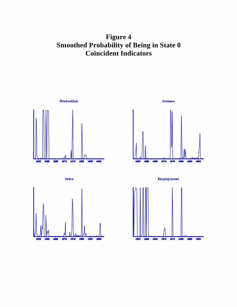
Figure 4Smoothed Probability of Being in State 0

Coincident Indicators

1. See Diebold and Rudebusch (1992) for further discussion of the role of comovement in

determining business-cycle turning points.

2. In the frequency domain, Sargent (1987, p. 282) offers the following update of Burns and

Mitchell's definition: ". . . the business cycle is the phenomenon of a number of important

economic aggregates (such as GNP, unemployment, and layoffs) being characterized by high

pairwise coherences at the low business cycle frequencies."

3. It is interesting to note that parallel structures may exist in many financial markets, which

makes sense to the extent that asset prices accurately reflect fundamentals, which themselves

have factor structure. See Singleton (1980), Bollerslev, Engle and Wooldridge (1988), and

Diebold and Nerlove (1989), among others, for examples of factor structure in both the

conditional means and conditional variances of various asset returns.

4. Again, parallel structures may exist in financial markets. Regime switching has been

found, for example, in the conditional mean dynamics of interest rates (Hamilton, 1988;

Cecchetti, Lam and Mark, 1990) and exchange rates (Engel and Hamilton, 1990), and in the

conditional variance dynamics of stock returns (Hamilton and Susmel, 1994).

5. Key early contributions include the early work of Quandt (1958) and Goldfeld and Quandt

(1973).

6. The ij-th element of M gives the probability of moving from state i (at time t-1) to state j (at

time t). Note that there are only two free parameters, the "staying probabilities" p and p .00 11

7. See also De Toldi, Gourieroux and Monfort (1992).

8. Consumption appears in both of the last two equations in order to capture both its durable

and nondurable aspects.

9. See Sargent (1989), and Hansen and Sargent (1993), among others.

10. See, for example, Kydland and Prescott (1982), Hansen (1985), Cooley and Hansen

(1989), and Cooley (1995).

11. Durlauf (1991) and Cooper and Durlauf (1993) provide insightful discussion of this point.

Footnotes

12. In many respects, such equilibria are reminiscent of the traditional Keynesian regimes of

"full employment" and "underemployment" discussed, for example, in DeLong and Summers

(1988).

13. Related approaches have been proposed by Durlauf (1995) and Evans and Honkapohja

(1993), among others.

14. Each of the four component indicators is graphed on a different scale to enable their

presentation in one graph. For this reason, no scale appears on the vertical axis of the graph.

15. Stock and Watson motivate and derive their index in precisely this way. The Commerce

indexes are attempts at the same methodology, albeit less formally.

16. We give the startup values for iteration in the first column of Table 2.

17. They follow the NBER chronology closely, for example.

18. Again, we use the startup values shown in the first column of Table 2.

19. See Hamilton's (1994) survey, and the many papers cited there.

20. The results of Giné and Zinn (1990) and Stinchcombe and White (1993), used by Diebold

and Chen (1996) to argue the validity of the bootstrap in Andrews' (1993) case, are relevant

here as well.

21. The null distribution depends, even asymptotically, on the (unknown) true value of the

autoregressive parameter. Fortunately, however, the dependence is slight; for example,

Garcia's one percent critical values only vary from 11.54 to 11.95 over an autoregressive

parameter range of -0.5 to 0.8.

22. Moreover, countercyclical policy may itself introduce nonlinearities if it is applied only in

extreme situations. See Zarnowitz and Moore (1982) and Becketti and Haltiwanger (1987).