P1: FXS/ABE P2: FXS CHAPTER 17 - Cambridge University …downloads.cambridge.edu.au/education/extra/209/PageProofs/MMCAS...A continuous random variable is one that can take any value

P1: FXS/ABE P2: FXS

0521665175c17.xml CUAU030-EVANS August 27, 2008 6:57

C H A P T E R

17Continuous randomvariables and their

probability distributions

ObjectivesTo define continuous random variables.

To specify the distributions for continuous random variables using probability

density functions.

To calculate and interpret the expectation (mean), median, mode, variance and

standard deviation for a continuous random variable.

To relate the graph of a probability density function to the values of the

parameters defining that function.

To relate probabilities for intervals to the graph of a probability density function.

To use calculus to calculate probabilities for intervals for a probability density function.

To use technology to calculate probabilities for intervals for a probability density

function.

To apply knowledge of probability density functions for continuous random

variables to solve probability-related problems.

17.1 Continuous random variablesA continuous random variable is one that can take any value in an interval of the real number

line. For example, if X is the random variable which takes its values as ‘distance in metres’ that

a parachutist lands from a particular marker, then X is a continuous random variable, and here

the values which X may take are the non-negative real numbers.

A continuous random variable has no limit as to the accuracy with which it can be

measured. For example, let W be the random variable with values ‘a person’s weight in

kilograms’, and Wi be the random variable with values ‘a person’s weight in kilograms

measured to the ith decimal place’.

594Cambridge University Press • Uncorrected Sample Pages • 2008 © Evans, Lipson, Jones, Avery, TI-Nspire & Casio ClassPad material prepared in collaboration with Jan Honnens & David Hibbard

SAMPLE

P1: FXS/ABE P2: FXS


Chapter 17 — Continuous random variables and their probability distributions 595

Then: W0 = 83 implies 82.5 ≤ W < 83.5

W1 = 83.3 implies 83.25 ≤ W < 83.35

W2 = 83.28 implies 83.275 ≤ W < 83.285

W3 = 83.281 implies 83.2805 ≤ W < 83.2815

and so on. Thus, the random variable W cannot take an exact value, since it is always rounded

to the limits imposed by the method of measurement used. Hence, the probability of W being

exactly equal to a particular value is zero, and this is true for all continuous random variables.

That is,

Pr(W = w) = 0 for all w

In practice, considering W taking a particular value is equivalent to W taking a value in an

appropriate interval.

Thus, from above:

Pr(W0 = 83) = Pr(82.5 ≤ W < 83.5)

To determine the value of this probability you could begin by measuring the weight of a

large number of randomly chosen people, and determine the proportion of the people in the

group who have weights in this interval.

Suppose after doing this a histogram of weights was obtained as shown.

8382.5 83.5

Weights0

f (w)

From this histogram:

Pr(W0 = 83) = Pr(82.5 ≤ W < 83.5)

= shaded area from 82.5 to 83.5

total area

If the histogram is scaled so that the total area under the blocks is one, then:

P(W0 = 83) = Pr(82.5 ≤ W < 83.5)

= area under block from 82.5 to 83.5

Cambridge University Press • Uncorrected Sample Pages • 2008 © Evans, Lipson, Jones, Avery, TI-Nspire & Casio ClassPad material prepared in collaboration with Jan Honnens & David Hibbard

SAMPLE

P1: FXS/ABE P2: FXS


596 Essential Mathematical Methods 3 & 4 CAS

Suppose that the sample size gets larger and the class interval width gets smaller. If

theoretically this process is continued so that the intervals are arbitrarily small, the histogram

can be modelled by a smooth curve, as shown in the following diagram.

w

f (w)

8382.5 83.5

0

The curve obtained here is of great importance for a continuous random variable.

The function f whose graph models the histogram as the number of intervals is

increased is called the probability density function. The probability density function f

is used to describe the probability distribution of a continuous random variable, X.

Now, the probability of interest is no longer represented by the area under the histogram, but

the area under the curve. That is:

Pr(W0 = 83) = Pr(82.5 ≤ W < 83.5)

= area under the graph of the function with rule f (w) from 82.5 to 83.5

=∫ 83.5

82.5f (w)dw

In general, for the continuous random variable X with density function f:

Pr(a < X < b) =∫ b

af (x)dx is given by the area of the shaded region.

x0 a b

f (x)

In order to be a probability density function a function must satisfy certain conditions.


SAMPLE

P1: FXS/ABE P2: FXS



If the range of the continuous random variable X is [a, b] then the domain of its probability

density function f is [a, b]. The probability density function will satisfy two properties:

1 f (x) ≥ 0 for all x ∈ [a, b] and 2∫ b

af (x)dx = 1

Note that Pr(X < c) = Pr(X ≤ c)

=∫ c

af (x)dx

The probability density function does not give probabilities and f (x) may take values

greater than one. The probabilities are given by areas determined by the graph of f .

In many cases the range of X is an unbounded interval, for example [1, ∞) or indeed R.

Therefore, some new notation is necessary.

If the range of X is [1, ∞), then it would be required that the area of the region under the

graph of the probability density function be one. This can be expressed as∫ ∞

1f (x)dx = 1.

This is computed as limk→∞

∫ k

1f (x)dx . If the probability density function f has domain R, then∫ ∞

−∞f (x)dx = 1. This is computed as lim

k→∞

∫ k

−kf (x)dx .

Any probability density function f with domain [a, b] (or any other interval) may be

extended to a function with domain R by defining f ∗(x) = f (x) for all x ∈ [a, b] and

f ∗(x) = 0 for all x /∈ [a, b].

This leads to the following:

A probability density function (or its natural extension) satisfies the following two

properties:

1 f (x) ≥ 0 for all x 2∫ ∞

−∞f (x)dx = 1

Note that, since the probability of X taking any exact value is zero, then:

Pr(a < X < b) = Pr(a ≤ X < b) = Pr(a < X ≤ b) = Pr(a ≤ X ≤ b)

That is, there is no difference between the numerical values of all of these expressions.

Example 1

Suppose that the random variable X has the density function with the rule:

f (x) ={

cx 0 ≤ x ≤ 2

0 if x > 2 or x < 0

a Find the value of c that makes f a probability density function.

b Find Pr(X > 1.5).


SAMPLE

P1: FXS/ABE P2: FXS



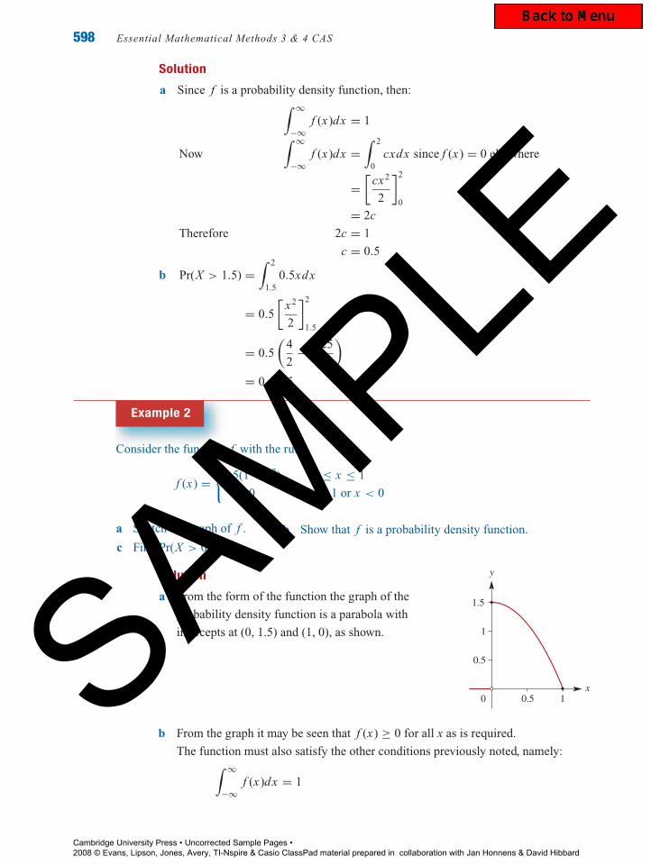
Solution

a Since f is a probability density function, then:∫ ∞

−∞f (x)dx = 1

Now∫ ∞

−∞f (x)dx =

∫ 2

0cxdx since f (x) = 0 elsewhere

=[

cx2

2

]2

0

= 2c

Therefore 2c = 1

c = 0.5

b Pr(X > 1.5) =∫ 2

1.50.5xdx

= 0.5

[x2

2

]2

1.5

= 0.5

(4

2− 2.25

2

)= 0.4375

Example 2

Consider the function f with the rule:

f (x) ={

1.5(1 − x2) 0 ≤ x ≤ 1

0 if x > 1 or x < 0

a Sketch the graph of f . b Show that f is a probability density function.

c Find Pr(X > 0.5).

Solution

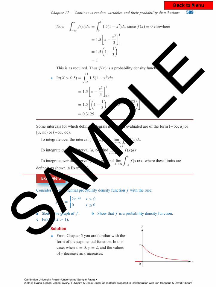
a From the form of the function the graph of the

probability density function is a parabola with

intercepts at (0, 1.5) and (1, 0), as shown.

x

y

1.5

1

1

0.5

0 0.5

b From the graph it may be seen that f (x) ≥ 0 for all x as is required.

The function must also satisfy the other conditions previously noted, namely:∫ ∞

−∞f (x)dx = 1


SAMPLE

P1: FXS/ABE P2: FXS



Now∫ ∞

−∞f (x)dx =

∫ 1

01.5(1 − x2)dx since f (x) = 0 elsewhere

= 1.5

[x − x3

3

]1

0

= 1.5

(1 − 1

3

)= 1

This is as required. Thus f (x) is a probability density function.

c Pr(X > 0.5) =∫ 1

0.51.5(1 − x2)dx

= 1.5

[x − x3

3

]1

0.5

= 1.5

[(1 − 1

3

)−

(0.5 − 0.125

3

)]= 0.3125

Some intervals for which definite integrals need to be evaluated are of the form (−∞, a] or

[a, ∞) or (−∞, ∞).

To integrate over the interval (–∞, a] find limk→−∞

∫ a

kf (x)dx

To integrate over the interval [a, ∞] find limk→∞

∫ k

af (x)dx

To integrate over the interval (−∞, ∞) find limk→∞

∫ k

−kf (x)dx , where these limits are

defined, as shown in Example 3.

Example 3

Consider the exponential probability density function f with the rule:

f (x) ={

2e−2x x > 0

0 x ≤ 0

a Sketch the graph of f . b Show that f is a probability density function.

c Find Pr(X > 1).

Solution

a From Chapter 5 you are familiar with the

form of the exponential function. In this

case, when x = 0, y = 2, and the values

of y decrease as x increases.

x

y

2

0


SAMPLE

P1: FXS/ABE P2: FXS



b It is known that f (x) ≥ 0 for all x as required.

The second condition is that∫ ∞

−∞f (x)dx = 1

Now∫ ∞

−∞2e−2x dx =

∫ ∞

02e−2x dx , since f (x) = 0 for x ≤ 0

To evaluate this integral, consider limk→∞

∫ k

02e−2x dx

= limk→∞

[2e−2x

−2

]k

0

= limk→∞

[−e−2x]k

0

= limk→∞

(−e−2k) − (−e−0)

= 0 + e−0

= 1

Thus f satisfies the requirements of a probability density function.

c Pr(X > 1) = limk→∞

∫ k

12e−2x dx

= limk→∞

[2e−2x

−2

]k

1

= limk→∞

[−e−2x]k

1

= limk→∞

(−e−2k) − (−e−2)

= 0 + e−2

= 1

e2

= 0.1353, correct to four decimal places

Using the TI-NspireThis is an application of integration.

a The graph is as shown.


SAMPLE

P1: FXS/ABE P2: FXS



b and c The required integrations are

performed to achieve the results.

∞, the symbol for infinity, can be found in

the catalog ( 4), or by typing / j.

Using the Casio ClassPadThis is an application of integration.

a The graph is as shown.

b and c The integrations are

performed to achieve the results.

Exercise 17A

1 Show that the function f with rule

f (x) =

24

x33 ≤ x ≤ 6

0 x < 3 or x > 6

is a probability density function.

2 Let X be a continuous random variable with the following probability density function:

f (x) ={

x2 + kx + 1 0 ≤ x ≤ 2

0 x < 0 or x > 2

Determine the constant k such that f is a valid probability density function.


SAMPLE

P1: FXS/ABE P2: FXS



3 Consider the random variable X having the probability density function with the rule:

f (x) ={

12x2(1 − x) 0 ≤ x ≤ 1

0 x < 0 or x > 1

a Sketch the graph of f (x). b Find Pr(X < 0.5).

c Shade the region which represents this probability on your sketch graph.

4 Consider the random variable Y with probability density function with the rule:

f (y) ={

ke−y y ≥ 0

0 y < 0

Find:

a the constant k b Pr(Y ≤ 2)

5 The quarantine period for a certain disease is between 5 and 11 days after contact. The

probability of showing the first symptoms at various times during the quarantine period is

described by the probability density function:

f (t) = 1

36(t − 5)(11 − t)

a Sketch the graph of the function.

b Find the probability that the symptoms will appear within 7 days of contact.

6 A probability model for the mass x kg of a 2-year-old child is given by:

f (x) = k sin

[1

10�(x − 7)

], 7 ≤ x ≤ 17

a Show that k = 1

20�.

b Hence find the percentage of 2-year-olds whose mass is:

i greater than 16 kg ii between 12 and 13 kg

7 A probability density function for the lifetime t hours of Electra light globes is given by

the rule:

f (t) = ke(− t200 ), t > 0

Find:

a the value of the constant k

b the probability that a bulb will last more than 1000 hours


SAMPLE

P1: FXS/ABE P2: FXS



8 A probability density function has a probability density function given by

f (x) =

k(1 + x) −1 ≤ x ≤ 0

k(1 − x) 0 < x ≤ 1

0 x < −1 or x > 1

where k > 0.

a Sketch the probability density function. b Evaluate k.

c Find the probability that X lies between −0.5 and 0.5.

9 Let X be a continuous random variable with probability density function given by:

f (x) ={

3x2 0 ≤ x ≤ 1

0 x < 0 or x > 1

a Sketch the graph of f (x).

b Find Pr(0.25 < X < 0.75) and sketch this on your graph.

10 A random variable X has a probability density function f with the rule:

f (x) =

1

100(10 + x) −10 < x ≤ 0

1

100(10 − x) 0 < x ≤ 10

0 x ≤ −10 or x > 10

a Sketch the graph of f . b Find Pr(−1 ≤ X < 1).

11 The life in hours, X, of a type of light globe has a probability density function with the

rule:

f (x) =

k

x2x > 1000

0 x ≤ 1000

a Evaluate k. b Calculate the probability the globe will last at least 2000 hours.

12 The weekly demand for petrol, X (in thousands of litres), at a particular service station is a

random variable with probability density function:

f (x) =2

(1 − 1

x2

)1 ≤ x ≤ 2

0 x < 1 or x > 2

a Determine the probability that more than 1.5 thousand litres are demanded in 1 week.

b Determine the probability that the demand for petrol in 1 week is less than

1.8 thousand litres, given than it is more than 1.5 thousand litres.


SAMPLE

P1: FXS/ABE P2: FXS



13 The length of time, X (in minutes), between the arrival of customers at an autobank is a

random variable with probability density function:

f (x) =

1

5e− x

5 x ≥ 0

0 x < 0

a Find the probability that more than 8 minutes elapses between successive customers.

b Find the probability that more than 12 minutes elapses between successive customers,

given that more than 8 minutes has passed.

14 A random variable X has density function given by:

f (x) =

0.2 −1 < x ≤ 0

0.2 + 1.2x 0 < x ≤ 1

0 x ≤ −1 or x > 1

a Find Pr(X ≤ 0.5). b Hence find Pr(X > 0.5|X > 0.1).

15 The continuous random variable X has probability density function f given by:

f (x) ={

e−x x ≥ 0

0 x < 0

a Sketch the graph of f .

b Find:

i Pr(X < 0.5) ii Pr(X ≥ 1) iii Pr(X ≥ 1|X > 0.5)

16 The continuous random variable X has probability density function f given by

f (x) ={

|ax | −2 ≤ x ≤ 2

0 x < −2 or x > 2

where a is a constant.

a Sketch the graph of f. b Hence or otherwise, find the value of a.

17.2 Cumulative distribution functions∗Another function of importance in describing a continuous random variable is the

cumulative distribution function F, or CDF. For a continuous random variable X, with

probability density function f , the cumulative distribution function defined on an interval

[a, b] is given by

f (x) = Pr(X ≤ x)

=∫ x

af (t)dt

where f is the probability density function and t is the variable of integration.

∗ Cumulative distribution functions are not mentioned explicitly in the Mathematical Methods Units 3 and 4 CAS studydesign but are useful in our study of continuous probability distributions.


SAMPLE

P1: FXS/ABE P2: FXS



For the probability density function defined on R:

f (x) = Pr(X ≤ x)

=∫ x

−∞f (t)dt

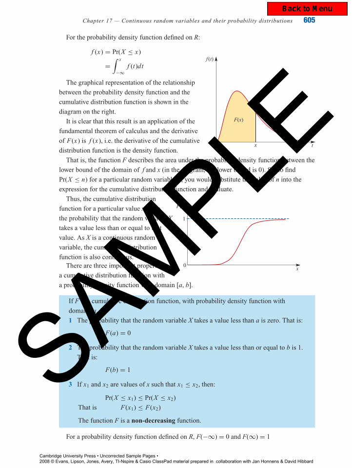
The graphical representation of the relationship

between the probability density function and the

cumulative distribution function is shown in the

diagram on the right.

f (t)

F(x)

tx

It is clear that this result is an application of the

fundamental theorem of calculus and the derivative

of F(x) is f (x), i.e. the derivative of the cumulative

distribution function is the density function.

That is, the function F describes the area under the probability density function between the

lower bound of the domain of f and x (in the diagram, the lower bound is 0). So, to find

Pr(X ≤ n) for a particular random variable X, you would substitute the value of n into the

expression for the cumulative distribution function and evaluate.

Thus, the cumulative distribution

function for a particular value x gives

the probability that the random variable X

takes a value less than or equal to that

value. As X is a continuous random

variable, the cumulative distribution

function is also continuous.0

F(x)

x

1

There are three important properties of

a cumulative distribution function with

a probability density function with domain [a, b].

If F is a cumulative distribution function, with probability density function with

domain [a, b]:

1 The probability that the random variable X takes a value less than a is zero. That is:

F(a) = 0

2 The probability that the random variable X takes a value less than or equal to b is 1.

That is:

F(b) = 1

3 If x1 and x2 are values of x such that x1 ≤ x2, then:

Pr(X ≤ x1) ≤ Pr(X ≤ x2)

That is F(x1) ≤ F(x2)

The function F is a non-decreasing function.

For a probability density function defined on R, F(−∞) = 0 and F(∞) = 1


SAMPLE

P1: FXS/ABE P2: FXS



Example 4

The time (in seconds) it takes a student to complete a puzzle is a random variable with a

density function with the rule:

f (x) =

5

x2x ≥ 5

0 x < 5

Find F(x), the cumulative distribution function of X.

Solution

F(x) =∫ x

5f (t)dt

=∫ x

5

5

t2

=[−5

t

]x

5

= −5

x+ 1

That is: F(x) = 1 − 5

x

The importance of the cumulative distribution function is that probabilities for

various intervals can be computed directly from F(x).

Example 5

Use the cumulative distribution function found in Example 4 to find:

a the probability that a student takes less than 12 seconds to complete the puzzle

b the probability that a student takes between 8 and 10 seconds to complete the puzzle, given

that he takes less than 12 seconds

Solution

a Pr(X ≤ 12) can be obtained by substituting 12 in the expression for F(x).

F(12) = 1 − 5

12

= 7

12


SAMPLE

P1: FXS/ABE P2: FXS



b Pr(8 ≤ X ≤ 10|X ≤ 12) = Pr(8 ≤ X ≤ 10 ∩ X ≤ 12)

Pr(X ≤ 12)= Pr(8 ≤ X ≤ 10)

Pr(X ≤ 12)

= F(10) − F(8)

F(12)

=1

2− 3

87

12

= 3

14

Exercise 17B

1 The probability density function for a random variable X is:

f (x) =

1

50 < x < 5

0 x ≤ 0 or x ≥ 5

a Find F(x), the cumulative distribution function of X. b Hence find Pr(X ≤ 3).

2 A random variable X has a cumulative distribution function:

F(x) ={

0 x < 0

1 − e−x2x ≥ 0

a Sketch the graph of F(x). b Find Pr(X ≥ 2).

c Find Pr(X ≥ 2|X < 3).

3 The continuous random variable X has cumulative distribution function F given by:

F(x) =

0 x < 0

kx2 0 ≤ x ≤ 6

1 x > 6

a Determine the value of the constant k. b Calculate Pr

(1

2≤ X ≤ 1

).

17.3 Mean, median and mode for a continuousrandom variableThe centre is an important summary

feature of a probability distribution.

The diagram shows two

probability distributions which are

identical except for their centres.

f (x)

x

More than one measure of centre may be determined for a continuous random variable, and

each gives useful information about the random variable under consideration. The most

generally useful measure of centre is the mean.


SAMPLE

P1: FXS/ABE P2: FXS



MeanIn the same way as the mean or expected value for a discrete random variable is defined, one

can define the mean or expected value for a continuous random variable.

The mean or expected value of a continuous random variable X is given by:

E(X ) =∫ ∞

−∞x f (x) dx

provided the integral exists. As in the case of a discrete random variable the mean is

always denoted by the Greek letter � (mu).

If f (x) = 0 for all x /∈ [a, b], then E(X ) =∫ b

ax f (x)dx

This definition is consistent with the definition of the expected value for a discrete random

variable. As in the case of a discrete random variable, the mean or expected value of a

continuous random variable is not necessarily the value the random variable takes in any

particular experiment, but the long-run average value of the variable. As an example, consider

the daily demand for petrol at a service station. The mean of this variable tells us the average

daily demand for petrol over a very long period of time.

Example 6

Find the expected value of the random variable X which has probability density function with

rule:

f (x) ={

0.5x 0 ≤ x ≤ 2

0 x < 0 or x > 2

SolutionBy definition E(X ) =

∫ ∞

−∞x f (x)dx

=∫ 2

0x × 0.5xdx since f (x) = 0 elsewhere

= 0.5∫ 2

0x2dx

= 0.5

[x3

3

]2

0

= 4

3

The mean of a function of X is defined as follows. (In this case the function of X is denoted as

g(X ) and is the composition of the random variable X and the function g.)


SAMPLE

P1: FXS/ABE P2: FXS



The expected value of g(X ) is

E[g(X )] =∫ ∞

−∞g(x) f (x) dx

provided the integral exists.

Generally, as in the case of a discrete random variable, the expected value of a function of X

is not equal to that function of the expected value of X. That is:

E{g(x)} �= g{E(X )}

Example 7

If X is the random variable with probability density function f :

f (x) ={

0.5x 0 ≤ x ≤ 2

0 x < 0 or x > 2

Find:

a the expected value of X2 b the expected value of ex (correct to four decimal places)

Solution

a E[X2] =∫ ∞

−∞x2 f (x)dx

=∫ 2

0x2 × 0.5xdx since f (x) = 0 elsewhere

= 0.5∫ 2

0x3dx

= 0.5

[x4

4

]2

0

= 2

b E[ex ] =∫ ∞

−∞ex f (x)dx

=∫ 2

0ex f (x)dx since f (x) = 0 elsewhere

=∫ 2

0ex × 0.5xdx

= 4.195 (correct to three decimal places)

A case where the equality does hold is where g is a linear function of X. Then

E(aX + b) = aE(X ) + b (a, b constant)

Percentiles and the medianAnother value of interest is the value of X which bounds a particular area under a probability

density function. For example, a teacher may wish determine the mark (p) below which lie


SAMPLE

P1: FXS/ABE P2: FXS



75% of all students’ marks. This is called the 75th percentile of the population, and is found by

solving: ∫ p

−∞f (x)dx = 0.75

This can be stated more generally.

The value p of X which is the solution of an equation of the form∫ p

−∞f (x)dx = q

is called a percentile of the distribution. Here q is the required percentile. (For the

example above q = 75% = 0.75.)

Example 8

The duration of telephone calls to the order department of a large company is a random

variable X minutes with probability density function:

f (x) =

1

3e− x

3 x > 0

0 x ≤ 0

Find the value of a such that 90% of phone calls last less than a minutes.

Solution

To find the value of a, solve the equation:∫ a

0

1

3e− x

3 dx = 0.90

That is,[−e− x

3

]a

0= 0.90

∴ 1 − e− a3 = 0.90

∴ −a

3= loge 0.10

∴ a = 3 loge (10)

= 6.908 (correct to three decimal places)

So 90% of the calls to this company last less than 6.908 minutes.

As for discrete probability distributions, a percentile of special interest is the median, or 50th

percentile. The median is the middle value of the distribution. That is, the probability of X

taking a value below the median is 0.5, and the probability of X taking a value above the

median is 0.5. Thus, if m is the median value of the distribution, then:

Pr(X ≤ m) = Pr(X > m)

= 0.5


SAMPLE

P1: FXS/ABE P2: FXS



The median may be determined readily from the cumulative distribution function, as it is the

50th percentile of the distribution. Graphically, the median is the value of the random variable

which divides the area under the probability density function in half.

The median is another measure of centre of

a continuous probability distribution.

The median, m, of a probability distribution

function is the value of X such that:∫ m

−∞f (x)dx = 0.5

f (x)

xm

0.5

Example 9

Suppose the probability density function of weekly sales of topsoil, X (in tonnes), is given by

the rule:

f (x) ={

2(1 − x) 0 ≤ x ≤ 1

0 x < 0 or x > 1

Find the median value of X, and interpret.

Solution

The solution here is the value of m such that:∫ m

02(1 − x) = 0.5

∴ 2

[x − x2

2

]m

0

= 0.5

∴ 2m − m2 = 0.5

∴ m2 − 2m + 0.5 = 0

m = 0.293 or 1.707

But since 0 ≤ x ≤ 1 the median m = 0.293 tonnes. That is, in the long run, 50% of

weekly sales will be less than 0.293 tonnes, and 50% will be more.

ModeAnother value of interest is the mode, M, of the distribution. Although not actually a measure

of centre the mode does tell us the most likely or most probable value of X. Thus, the mode

occurs at the maximum value of f (x), and may be located through considering the graph of

the probability density function.


SAMPLE

P1: FXS/ABE P2: FXS



If f is the probability density function of X,

then the mode, M, is the value of X

such that:

f (M) ≥ f (x) for all other x

f (x)

xM

Example 10

Find the mode of the continuous random variable X with probability density function:

f (x) ={

12x2(1 − x) 0 ≤ x ≤ 1

0 x < 0 or x > 1

Solution

To find the maximum value of f (x) in the interval [0,1], begin by expanding the

expression and then differentiating the function as follows:

f (x) = 12x2 − 12x3

Thus f ′(x) = 24x − 36x2

= 0

12x(2 − 3x) = 0

x = 0 or x = 2

3

Consideration of the function shows that x = 0 corresponds to a minimum value of

f (x), and x = 2

3corresponds to a maximum value of f (x). Thus the mode M = 2

3

f (x)

x123

0


SAMPLE

P1: FXS/ABE P2: FXS



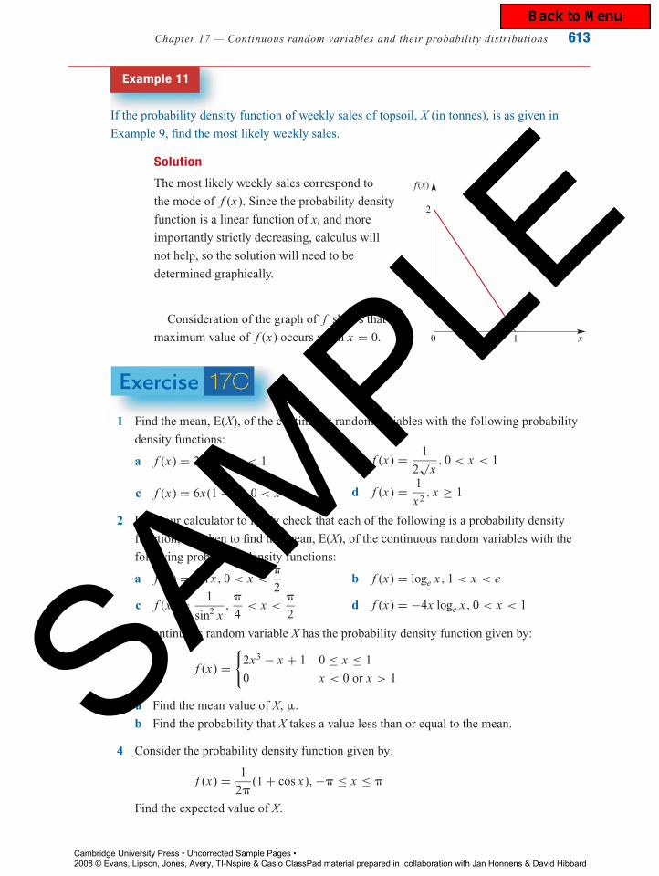
Example 11

If the probability density function of weekly sales of topsoil, X (in tonnes), is as given in

Example 9, find the most likely weekly sales.

Solution

The most likely weekly sales correspond to

the mode of f (x). Since the probability density

function is a linear function of x, and more

importantly strictly decreasing, calculus will

not help, so the solution will need to be

determined graphically.

f(x)

x

2

10

Consideration of the graph of f shows that the

maximum value of f (x) occurs when x = 0.

Exercise 17C

1 Find the mean, E(X), of the continuous random variables with the following probability

density functions:

a f (x) = 2x, 0 < x < 1 b f (x) = 1

2√

x, 0 < x < 1

c f (x) = 6x(1 − x), 0 < x < 1 d f (x) = 1

x2, x ≥ 1

2 Use your calculator to firstly check that each of the following is a probability density

function, and then to find the mean, E(X), of the continuous random variables with the

following probability density functions:

a f (x) = sin x, 0 < x <�

2b f (x) = loge x, 1 < x < e

c f (x) = 1

sin2 x,

�

4< x <

�

2d f (x) = −4x loge x, 0 < x < 1

3 A continuous random variable X has the probability density function given by:

f (x) ={

2x3 − x + 1 0 ≤ x ≤ 1

0 x < 0 or x > 1

a Find the mean value of X, �.

b Find the probability that X takes a value less than or equal to the mean.

4 Consider the probability density function given by:

f (x) = 1

2�(1 + cos x), −� ≤ x ≤ �

Find the expected value of X.


SAMPLE

P1: FXS/ABE P2: FXS



5 A random variable Y has a probability density function:

f ( y) ={

Ay 0 ≤ y ≤ B

0 x < 0 or x > B

Find A and B if the mean of Y is 2.

6 A random variable X has the probability density function given by:

f (x) ={

12x2(1 − x) 0 ≤ x ≤ 1

0 x < 0 or x > 1

Find:

a E

(1

X

)b E(ex )

7 The random variable X has a probability density function given by:

f (x) ={

k 0 ≤ x ≤ 1

0 x < 0 or x > 1

Find:

a the value of k b the median, m, of X

8 The time X seconds between arrivals of particles at a radiation counter has been found to

have a probability density function f with the rule:

f (x) ={

0 x < 0

e−x x ≥ 0

Find:

a Pr(X ≤ 1) b Pr(1 ≤ X ≤ 2) c the median, m, of X

9 A continuous random variable has a probability density function given by:

f (x) ={

5(1 − x)4 0 ≤ x ≤ 1

0 x < 0 or x > 1

Find the median, m, of X (correct to four decimal places).

10 Suppose that the time (in minutes) between telephone calls received at a pizza restaurant

has probability density function:

f (x) =

1

4e− x

4 x ≥ 0

0 x < 0

Find the median time between calls.


SAMPLE

P1: FXS/ABE P2: FXS



11 The cumulative distribution function∗ of a continuous random variable X, F(x), is given

by:

F(x) =

0

4x3 − 3x4

1

x < 0

0 ≤ x ≤ 1

x > 1

Find:

a the probability density function of X b the mode, M, of X

12 A random variable X has a probability density function:

f (x) =

1

2sin x 0 < x < �

0 x ≤ 0 or x ≥ �

Find the mode, M, of X.

13 A continuous random variable X has the probability density function given by:

f (x) =

x 0 ≤ x < 1

2 − x 1 ≤ x < 2

0 x < 0 or x ≥ 2

a Find �, the expected value of X. b Find m, the median value of X.

c Find M, the mode of X.

14 Let the probability density function of X be:

f (x) ={

30x4(1 − x) 0 < x < 1

0 x < 0 or x ≥ 1

a Find the expected value of X, �.

b Find the median value of X, m, and hence show that the mean is less than the median.

15 A probability model for the mass x kg of a 2-year-old child is given by:

f (x) = 1

20� sin

[1

10�(x − 7)

], 7 ≤ x ≤ 17

a Find the mode of X, M. b Find the median value of X, m.

16 A random variable X has density function given by:

f (x) =

0.2 −1 < x ≤ 0

0.2 + 1.2x 0 < x ≤ 1

0 x < −1 or x > 1

a Find �, the expected value of X. b Find m, the median value of X.

c Find M, the mode of X.

∗ Cumulative distribution functions are not mentioned explicitly in the Mathematical Methods Units 3 and 4 CAS studydesign but are useful in our study of continuous probability distributions.


SAMPLE

P1: FXS/ABE P2: FXS



17 The exponential probability distribution describes the distribution of the time between

random events, such as phone calls. The general form of the exponential distribution with

parameter � is:

f (x) =

1

�e− x

� x ≥ 0

0 x < 0

a Differentiate kxe−kx and hence find an antiderivative of kxe−kx.

b Show that the mean of an exponential random variable is �.

c On the same axes, sketch the graph of an exponential random variable for:

i � = 1

2ii � = 1 iii � = 2

d Describe the effect of the variation of the parameter � on the graph of the distribution.

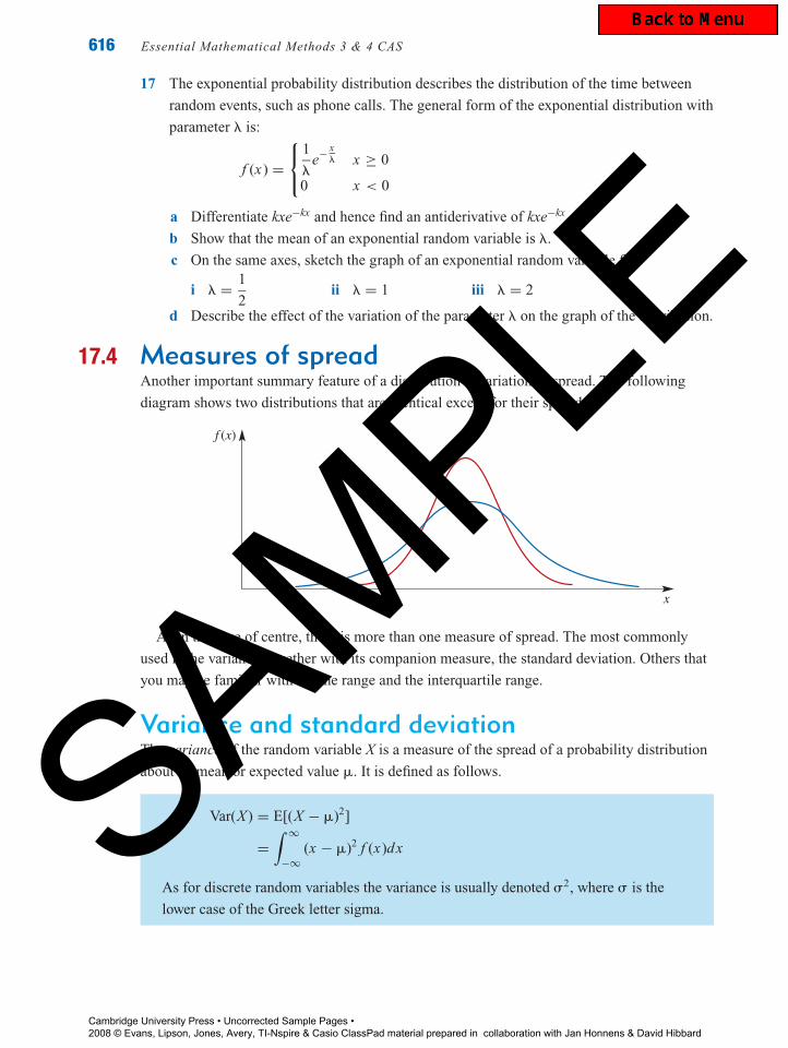
17.4 Measures of spreadAnother important summary feature of a distribution is variation or spread. The following

diagram shows two distributions that are identical except for their spreads.

x

f (x)

As in the case of centre, there is more than one measure of spread. The most commonly

used is the variance, together with its companion measure, the standard deviation. Others that

you may be familiar with are the range and the interquartile range.

Variance and standard deviationThe variance of the random variable X is a measure of the spread of a probability distribution

about its mean or expected value �. It is defined as follows.

Var(X ) = E[(X − �)2]

=∫ ∞

−∞(x − �)2 f (x)dx

As for discrete random variables the variance is usually denoted �2, where � is the

lower case of the Greek letter sigma.


SAMPLE

P1: FXS/ABE P2: FXS



Variance may be considered as the long-run average value of the square of the distance from

the values of X to �. Since the variance is determined by squaring the distance from the values

of X to � it is no longer in the units of measurement of the original random variable. A

measure of spread in the appropriate unit is found by taking the square root of the variance.

The standard deviation of X is defined as:

sd(X ) =√

Var(X )

The standard deviation is usually denoted �.

As in the case of discrete random variables, an alternative (computational) formula for

variance is generally used.

To calculate variance, use:

Var(X ) = E(X2) − �2

The computational form of the expression for variance is derived as follows:

Var(X ) =∫ ∞

−∞(x − �)2 f (x)dx

=∫ ∞

−∞(x2 − 2�x + �2) f (x)dx

=∫ ∞

−∞x2 f (x)dx −

∫ ∞

−∞2�x f (x)dx +

∫ ∞

−∞�2 f (x)dx

= E(X2) − 2�

∫ ∞

−∞x f (x)dx + �2

∫ ∞

−∞f (x)dx

Since∫ ∞

−∞x f (x)dx = � and

∫ ∞

−∞f (x)dx = 1

Var(X ) = E(X2) − 2�2 + �2

= E(X2) − �2

Example 12

Find the variance and standard deviation of the random variable X which has the probability

density function f with rule:

f (x) ={

0.5x 0 ≤ x ≤ 2

0 x < 0 or x > 2


SAMPLE

P1: FXS/ABE P2: FXS



Solution

Use the computational formula Var(X ) = E(X2) − �2

First, evaluate E(X2):

E(X2) =∫ ∞

−∞x2 f (x)dx

=∫ 2

0x2× 0.5xdx

= 0.5∫ 2

0x3dx

= 0.5

[x4

4

]2

0

= 0.5 × 4

= 2

Now E(X ) = 4

3(from Example 6)

so Var(X ) = 2 −(

4

3

)2

= 2

9

and sd(X ) =√

2

9

=√

2

3or, correct to three decimal places, 0.471

It helps to make the standard deviation more meaningful to give it an interpretation which

relates to the probability distribution. As already stated for discrete random variables, it is also

the case for many continuous random variables that about 95% of the distribution lies within

two standard deviations either side of the mean.

In general, for many continuous random variables X:

Pr(� − 2� ≤ X ≤ � + 2�) ≈ 0.95

Example 13

The life of a certain brand of battery, X, is a continuous random variable with mean 50 hours

and variance 16 hours. Find an (approximate) interval for the time period for which 95% of the

batteries would be expected to last.

Solution

Pr(� − 2� ≤ X ≤ � + 2�) ≈ 0.95. In this case � = 50 and � = √16 = 4, so one

could expect 95% of the batteries to last between 42 hours and 58 hours.


SAMPLE

P1: FXS/ABE P2: FXS



RangeThe range of a random variable is the difference between the smallest and the largest value the

variable may take, and is clearly determined from the domain of the probability density

function.

Example 14

Determine the range of the random variable X which has the probability density function:

f (x) =

1

9(4x − x2) 0 ≤ x ≤ 3

0 x < 0 or x > 3

Solution

From the probability density function X may take values from 0 to 3. Thus:

range of X = 3 − 0

= 3

Interquartile rangeThe interquartile range is the range of the middle 50% of the distribution. It is the difference

between the 75th percentile, also known as Q3, and the 25th percentile, also known as Q1.

Example 15

Determine the interquartile range of the random variable X which has the probability density

function:

f (x) ={

2x 0 ≤ x ≤ 1

0 x < 0 or x > 1

Solution

To find the 25th percentile a, solve:∫ a

02xdx = 0.25 ⇒ [x2]a

0 = 0.25 ⇒ a2 = 0.25 ⇒ a =√

0.25 = 0.5

To find the 75th percentile b, solve:∫ b

02xdx = 0.75 ⇒ [x2]b

0 = 0.75 ⇒ b2 = 0.75 ⇒ b =√

0.75 = 0.866,

correct to three decimal places

Thus the interquartile range is 0.866 − 0.5 = 0.366, correct to three decimal places.

Note that the negative solutions to each of these equations were not appropriate, as

0 ≤ x ≤ 1.


SAMPLE

P1: FXS/ABE P2: FXS



Exercise 17D

1 A continuous random variable X has a probability density function given by:

f (x) ={

3x2 0 ≤ x ≤ 1

0 x < 0 or x > 1

Find:

a a such that Pr(X ≤ a) = 0.25 b b such that Pr(X ≤ b) = 0.75

c the interquartile range of X

2 Given that the random variable X has probability density function:

f (x) ={

2x 0 < x < 1

0 x ≤ 0 or x ≥ 1

a Find the interquartile range of X.

b Find the variance of X, and hence the standard deviation of X.

3 If the random variable X has probability density function given by:

f (x) ={

0.5ex x ≤ 0

0.5e−x x > 0

a Sketch the graph of y = f (x)

b Find the interquartile range of X, giving your answer correct to three decimal places.

4 The continuous random variable X has probability density function given by:

f (x) =

k

x1 ≤ x ≤ 9

0 x < 1 or x > 9

a Find the value of k.

b Find the mean and variance of X, giving your answer correct to three decimal places.

5 The continuous random variable X has density function f given by:

f (x) =

0 x < 0

2 − 2x 0 ≤ x ≤ 1

0 x > 1

a Find the interquartile range of X. b Find the mean and variance of X.

6 A random variable X has probability density function f with the rule:

f (x) ={

0 x < 0

2xe−x2x ≥ 0

Find the interquartile range of X.


SAMPLE

P1: FXS/ABE P2: FXS



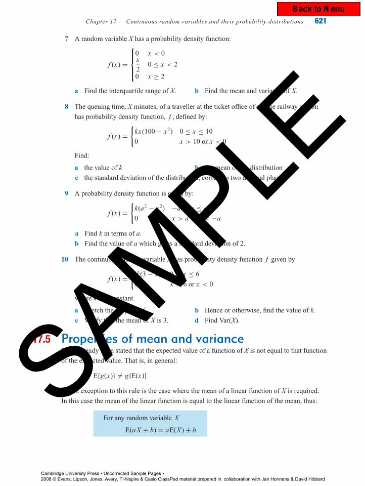
7 A random variable X has a probability density function:

f (x) =

0 x < 0x

20 ≤ x < 2

0 x ≥ 2

a Find the interquartile range of X. b Find the mean and variance of X.

8 The queuing time, X minutes, of a traveller at the ticket office of a large railway station

has probability density function, f , defined by:

f (x) ={

kx(100 − x2) 0 ≤ x ≤ 10

0 x > 10 or x < 0

Find:

a the value of k b the mean of the distribution

c the standard deviation of the distribution, correct to two decimal places.

9 A probability density function is given by:

f (x) ={

k(a2 − x2) −a ≤ x ≤ a

0 x > a or x < −a

a Find k in terms of a.

b Find the value of a which gives a standard deviation of 2.

10 The continuous random variable X has probability density function f given by

f (x) ={

|k(3 − x)| 0 ≤ x ≤ 6

0 x > 6 or x < 0

where k is a constant.

a Sketch the graph of f . b Hence or otherwise, find the value of k.

c Verify that the mean of X is 3. d Find Var(X).

17.5 Properties of mean and varianceIt has already been stated that the expected value of a function of X is not equal to that function

of the expected value. That is, in general:

E{g(x)} �= g{E(x)}An exception to this rule is the case where the mean of a linear function of X is required.

In this case the mean of the linear function is equal to the linear function of the mean, thus:

For any random variable X

E(aX + b) = aE(X ) + b


SAMPLE

P1: FXS/ABE P2: FXS



The validity of this statement can be readily demonstrated.

E(aX + b) =∫ ∞

−∞(ax + b) f (x)dx

=∫ ∞

−∞ax f (x)dx +

∫ ∞

−∞b f (x)dx

= a

∫ ∞

−∞x f (x)dx + b

∫ ∞

−∞f (x)dx

= aE(X ) + b, since∫ ∞

−∞f (x)dx = 1

Consider the variance of a linear function of X, Var(aX + b).

Var(aX + b) = E(aX + b)2 − [E(aX + b)]2

Now [E(aX + b)]2 = [aE(X ) + b]2 = [a� + b]2 = a2�2 + 2ab� + b2

and E(aX + b)2 = E(a2 X2 + 2abX + b2)

= a2E(X2) + 2ab� + b2

Thus Var(aX + b) = a2E(X2) + 2ab� + b2 − a2�2 − 2ab� − b2

= a2E(X2) − a2�2

= a2Var(X )

That is:

For any random variable X :

Var(ax + b) = a2 Var(X )

Although initially the absence of b in the result may seem surprising, on reflection it makes

sense that adding a constant to X merely translates the probability density function of X, but

has no effect on the spread of the resultant distribution. If the random variable X has a

probability density function with the rule f (x), then the probability distribution with random

variable X + b has a corresponding probability density function with the rule f (x − b).

Similarly, multiplying by a is similar to a dilation by a factor of a, and this is consistent with

the answer obtained. However, there has to be an adjustment to determine the probability

density function of the random variable aX as the transformation must be area-preserving. This

is chosen as the function with the rule1

af( x

a

).

Thus if f (x) is the probability density function for the random variable X, then the

probability density function of the random variable aX + b is1

af

(x − b

a

). The

transformation is described by (x, y) →(

ax + b,y

a

). That is, if a and b are positive, a

dilation of factor a from the y-axis and1

afrom the x-axis and a translation of b units in the

positive direction of the x-axis.


SAMPLE

P1: FXS/ABE P2: FXS



Example 16

Suppose X is a continuous random variable with mean � = 10 and variance �2 = 2.

a Find E(2X + 1).

b Find Var(1 − 3X).

c If X has a probability density function with rule f (x), describe the rule for a probability

density function g, in terms of f for 2X + 1.

Solution

a E(2X + 1) = 2E(X ) + 1 = 2 × 10 + 1 = 21

b Var(1 − 3X ) = (−3)2Var(X ) = 9 × 2 = 18

c The rule is g(x) = 1

af

(x − b

a

)where a = 2 and b = 1. Therefore

g(x) = 1

2f

(x − 1

2

)

Sums of independent random variables*

In previous work the idea of independent events has been introduced. The term ‘independent’

is also applied to random variables. While a formal definition of independent random variables

is beyond the scope of this course, basically two random variables are independent if their joint

probability density function is a product of their individual probability density functions. This

is also true for their cumulative distribution functions. Knowing random variables

are independent allows us to make certain conclusions concerning their mean and variance.

Suppose X and Y are independent random variables; then:

E(X + Y ) = E(X ) + E(Y )

Var(X + Y ) = Var(X ) + Var(Y )

Note that in fact E(X + Y ) = E(X ) + E(Y ) whether or not X and Y are independent, but the

same cannot be said for variance.

Example 17

A manufacturing process involves two stages. The time taken to complete stage 1, X hours, is

a continuous random variable with mean � = 4 and standard deviation � = 1.5. The time

taken to complete stage 2, Y hours, is a continuous random variable with mean � = 7

and standard deviation � = 1. Find the mean and standard deviation of the total time taken

to complete the manufacturing process, if the times taken at each stage are

independent.

∗ This section covers material not included in the Mathematical Methods Units 3 and 4 CAS study design.


SAMPLE

P1: FXS/ABE P2: FXS



Solution

The total processing time is given by X + Y . To find the mean total processing time:

E(X + Y ) = E(X ) + E(Y )

= 4 + 7

= 11

Since X and Y are independent:

Var(X + Y ) = Var(X ) + Var(Y )

= (1.5)2 + (1)2

= 2.25 + 1

= 3.25

Hence the standard deviation of the total processing time is:

sd(X + Y ) =√

3.25

= 1.803

Exercise 17E

1 The amount of flour used each day in a bakery is a continuous random variable X with

mean of 4 tonnes. The cost of the flour is C = 300X + 100. Find E(C).

2 For certain glass ornaments the proportion of impurities per ornament, X, is a random

variable with a density function given by:

f (x) =

3x2

2+ x 0 ≤ x ≤ 1

0 x < 0 or x > 1

The value of each ornament (in dollars) is V = 100 − 1.5X

a Find E(X) and Var(X). b Hence find the mean and standard deviation of V.

3 Let X be a random variable with probability density function:

f (x) =

3x2

2−1 ≤ x ≤ 1

0 x < −1 or x > 1

Find:

a E(3X) and Var(3X) b E(3 − x) and Var(3 − X )

c the rule of a probability density function for 3X

4 The time spent waiting in line at a fast-food outlet is a continuous random variable X with

mean � = 2.5 minutes and standard deviation � = 1.5 minutes. The time taken for the fast

food to be prepared and served is a continuous random variable Y with mean � = 5

minutes and standard deviation � = 2.5 minutes.


SAMPLE

P1: FXS/ABE P2: FXS



a Find the mean and variance of the total time the customer waits for the order.

b Find the time interval within which about 95% of customers would wait.

5 The length of time Joan waits for her train to work each morning is a continuous random

variable with mean � = 7 minutes and standard deviation � = 2 minutes. If the time

waited each day is independent of the time waited any other day, find the mean and the

standard deviation of the total time waited each week (assume 5 working days per week).


SAMPLE

P1: FXS/ABE P2: FXS


Rev

iew


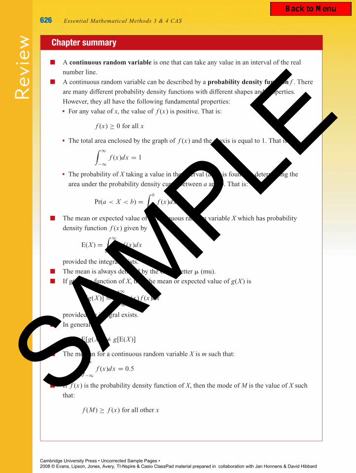
Chapter summary

A continuous random variable is one that can take any value in an interval of the real

number line.

A continuous random variable can be described by a probability density function f . There

are many different probability density functions with different shapes and properties.

However, they all have the following fundamental properties:� For any value of x, the value of f (x) is positive. That is:

f (x) ≥ 0 for all x

� The total area enclosed by the graph of f (x) and the x-axis is equal to 1. That is:∫ ∞

−∞f (x)dx = 1

� The probability of X taking a value in the interval (a, b) is found by determining the

area under the probability density curve between a and b. That is:

Pr(a < X < b) =∫ b

af (x)dx

The mean or expected value of a continuous random variable X which has probability

density function f (x) given by

E(X ) =∫ ∞

−∞x f (x)dx


The mean is always denoted by the Greek letter � (mu).

If g(X) is a function of X, then the mean or expected value of g(X ) is

E[g(X )] =∫ ∞

−∞g(x) f (x)dx


In general:

E[g(X )] �= g[E(X )]

The median for a continuous random variable X is m such that:∫ m

−∞f (x)dx = 0.5

If f (x) is the probability density function of X, then the mode of M is the value of X such

that:

f (M) ≥ f (x) for all other x


SAMPLE

P1: FXS/ABE P2: FXS


Review


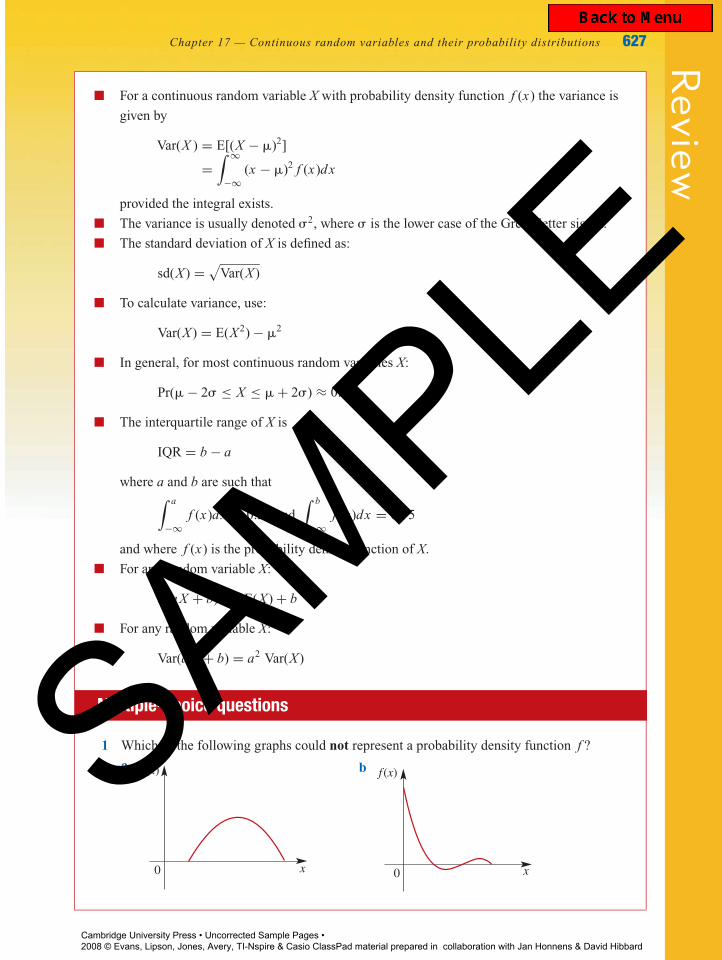
For a continuous random variable X with probability density function f (x) the variance is

given by

Var(X ) = E[(X − �)2]

=∫ ∞

−∞(x − �)2 f (x)dx


The variance is usually denoted �2, where � is the lower case of the Greek letter sigma.

The standard deviation of X is defined as:

sd(X ) =√

Var(X )

To calculate variance, use:

Var(X ) = E(X2) − �2

In general, for most continuous random variables X:

Pr(� − 2� ≤ X ≤ � + 2�) ≈ 0.95

The interquartile range of X is

IQR = b − a

where a and b are such that∫ a

−∞f (x)dx = 0.25 and

∫ b

−∞f (x)dx = 0.75

and where f (x) is the probability density function of X.

For any random variable X:

E(aX + b) = aE(X ) + b

For any random variable X:

Var(aX + b) = a2 Var(X )

Multiple-choice questions

1 Which of the following graphs could not represent a probability density function f ?

a

0

f (x)

x

b

0

f (x)

x


SAMPLE

P1: FXS/ABE P2: FXS


Rev

iew


c

0

f (x)

x

d

0

f (x)

x

e f (x)

x0

2 If the function f (x) = 4x represents a probability density function, then which of the

following could be the domain of f ?

A 0 < x < 0.25 B 0 < x < 0.5 C 0 < x < 1

D 0 < x <1√2

E1√2

< x <2√2

3 If a random variable X has probability density function

f (x) =

1

2sin x 0 < x < k

0 x ≥ k or x ≤ 0

then k is equal to:

A 1 B�

2C 2 D � E 2�

The following information relates to questions 4, 5 and 6.

A random variable X has probability density function:

f (x) =

3

4(x2 − 1) 1 < x < 2

0 x ≤ 1 or x ≥ 2

4 Pr(X ≤ 1.3) is closest to:

A 0.0743 B 0.4258 C 0.3 D 2.25 E 0.9258

5 The mean of X, E(X), is equal to:

A 1 B3

2C

9

4D

27

32E

27

16

6 The variance of X is:

A27

16B

67

1280C

81

16D

81

256E

729

256


SAMPLE

P1: FXS/ABE P2: FXS


Review


7 If a random variable X has a probability density function

f (x) =

x3

40 ≤ x ≤ 2

0 x > 2 or x < 0

then the median of X is closest to:

A 1.5 B 1.4142 C 1.6818 D 1.2600 E 1

8 If a random variable X has a probability density function

f (x) =

3

2(x − 1) (x − 2)2 1 ≤ x ≤ 3

0 x < 1 or x > 3

then the mode of X is:

A 1 B 1.333 C 2 D 2.6 E 3

9 If the consultation time (in minutes) at a surgery is represented by a random variable X,

which has probability density function

f (x) ={ x

40000(400 − x2) 0 ≤ x ≤ 20

0 x < 0 or x > 20

then the expected consultation time (in minutes) for three patients is:

A 102

3B 30 C 32 D 42 E 43

2

3

10 Suppose that the top 10% of students will be given an ‘A’ in mathematics. If the distribution

of scores on the examination is a random variable X with probability density function

f (x) ={ �

100sin

(�x

50

)0 ≤ x ≤ 50

0 x < 0 or x > 50

then the minimum score required to be awarded an ‘A’ is closest to:

A 40 B 41 C 42 D 43 E 44

Short-answer questions (technology-free)

1 The probability density function of X is given by:

f (x) ={

kx 1 ≤ x ≤ √2

0 otherwise

a Find k. b Find Pr(1 < X < 1.1). c Find Pr(1 < X < 1.2)

2 If the probability density function of X is given by:

f (x) ={

a + bx2 0 ≤ x ≤ 1

0 x > 1 or x < 0

and E(X ) = 2

3, find a and b.


SAMPLE

P1: FXS/ABE P2: FXS


Rev

iew



f (x) =

sin x

20 ≤ x ≤ �

0 x > � or x < 0

Find the median and mode of X.

4 The cumulative distribution function of X is given by:

F(x) =

1 x ≥ 51

4(x − 1) 1 ≤ x < 5

0 x < 1

a Find Pr(1 < X < 3). b Find Pr(X > 2|1 < X < 3). c Find Pr(X > 4|X > 2).

5 Consider the random variable X having the probability density function given by:

f (x) ={

12x2(1 − x) 0 ≤ x ≤ 1

0 otherwise

a Sketch the graph of y = f (x)

b Find Pr(X < 0.5) and illustrate this probability on your sketch graph.

6 The probability density function of a random variable X is:

f (x) ={

kx2(1 − x) 0 ≤ x ≤ 1

0 otherwise

a Determine k. b Find the mode of X .

c Find the probability that X is less than2

3.

d Find the probability that X is less than1

3, given that X is less than

2

3.

7 Y is a continuous random variable with probability density function:

f (y) ={

e−y, y ≥ 0

0, y < 0

Find:

a Pr(Y < 2) b Pr(Y < 3|Y > 1)

8 The cumulative distribution function of X is given by:

F(x) ={

loge x 1 ≤ x ≤ e

0 x > e or x < 1

a Find the median value of X. b Find the interquartile range of X.

c Find the probability density function of X, f (x).

9 The amount of fluid, X, in a can of soft drink is a continuous random variable with mean

330 mL and standard deviation 5 mL. Find an (approximate) interval for the amount of soft

drink contained in 95% of the cans.


SAMPLE

P1: FXS/ABE P2: FXS


Review


10 The weight, X, of cereal in a packet is a continuous random variable with mean 250 g and

variance 4 g. Find an (approximate) interval for the weight of cereal contained in 95% of

the packets.

Extended-response questions

1 The distribution of X, the life of a certain electronic component, in hours, is described by

the following probability density function:

f (x) ={ a

100

(1 − x

100

)100 < x < 1000

0 x ≤ 100 and x ≥ 1000

a What is the value of a? b Find the expected value of the life of the components.

c Find the cumulative distribution function, F(x), for this probability density function.

2 The continuous random variable X has cumulative distribution function given by:

F(x) =

0 x < 0

2x − x2 0 ≤ x ≤ 1

1 x > 1

a Find Pr(X > 0.5).

b Find a such that Pr(X < a) = 0.8.

c Find E(X) and E(√

X ).


f (x) ={ �

20cos

( �

10(x − 6)

)1 ≤ x ≤ 11

0 x < 1 or x > 11

a Find the median and interquartile range of X.

b Find the mean and the variance of X.

4 A hardware shop sells a certain size nail either in a small packet at $1.00 per packet, or

loose at $4.00 per kilogram. On any shopping day the number, X, of packets sold is a

binomial random variable with number of trials equal to 8 and probability of success of 0.6,

and the weight, Y kilograms, of nails sold loose is a continuous random variable with

probability density function f given by:

f (y) =

2( y − 1)

251 ≤ y ≤ 6

0 y < 1 or y > 6

a Find the probability that the weight of nails sold loose on any shopping day will be

between 4 kg and 5 kg.

b Calculate the expected money received on any shopping day from the sale of this size

nail in the store.


SAMPLE

P1: FXS/ABE P2: FXS


Rev

iew


5 The continuous random variable X has the probability density function f , where:

f (x) =

(x − 2)

22 ≤ x ≤ 4

0 x < 2 or x > 4

By first expanding (X − c)2, or otherwise, find two values of c such that:

E[(X − c)2] = 2

3

6 A wholesaler sells material offcuts in 5 m lengths. The amount, in metres, of unusable

material are the values of a random variable, X, with probability density function:

f (x) ={

k(x − 1)(3 − x) 1 ≤ x ≤ 3

0 x < 1 or x > 3

a Show that k = 0.75.

b Find the mean and variance of X.

c Find the probability that X is greater than 2.5 m.

7 The continuous random variable X has probability density function f , where:

f (x) =

k

12(x + 1)30 ≤ x ≤ 4

0 x < 0 or x > 4

CAS

C

ALCU LATOR

a Find k.

b Evaluate E(X + 1). Hence, find the mean of X.

c Use your calculator to verify your answer to part b.

d Find the value of c > 0 for which Pr(X ≤ c) = c.

8 The yield of a variety of corn has probability density function:

f (x) =

kx 0 ≤ x < 2

k(4 − x) 2 ≤ x < 4

0 x < 0 or x > 4

a Find k.

b Find the expected value, �, and variance of the yield of corn.

c Find the probability Pr(|X − �| < 1).

d Find the value of a such that Pr(X > a) = 0.6, giving your answer correct to one

decimal place.


SAMPLE

Documents

P1: FXS/ABE P2: FXS CHAPTER 17 - Cambridge University …downloads.cambridge.edu.au/education/extra/209/PageProofs/MMCAS...A continuous random variable is one that can take any value