24th February 2017 – XXIX cycle

POLITECNICO DI MILANO DEPARTMENT OF PHYSICS

DOCTORAL PROGRAMME IN PHYSICS

________________________

Anion intercalation in graphite:

a combined Electrochemical Atomic Force and Scanning

Tunneling Microscopy investigation

Doctoral Dissertation of:

Rossella Yivlialin

Supervisor:

Dr. Gianlorenzo Bussetti

Tutor:

Prof. Franco Ciccacci

The Chair of the Doctoral Program:

Prof. Paola Taroni

ii

To my parents

iii

ABSTRACT

Graphite electrodes have been, and continue to be, used largely in electrochemistry for a

wide range of applications from energy conversion or storage (e.g. lithium-ion batteries

and fuel cells) to electronic analysis (e.g. DNA analysis by carbon electronic chips) and in

a wide range of sizes, from micron or submicron to electrodes with extension of square

meters.

Electrochemistry has been connected to graphite since the early days of its research

activity because of its good electrical and thermal conductivity, corrosion resistance, low

thermal expansion, low elasticity and high purity. The more traditional form of graphite

implemented as electrode is the Highly Oriented Pyrolytic Graphite (HOPG) crystal.

Nowadays, HOPG has also focused an additional increasing interest due to its layered

structure, which can be thought in terms of a graphene sheet pile. In view of industrial

implementation, we are obliged to combine a quantity and quality enhancement of

graphene together with a reduction of the cost production. In these perspectives,

electrochemical strategies are successful. Graphite is delaminated by anion intercalation

inside the crystal at specific electrochemical potentials. Anions are placed in the inter-

layer region and they expand the graphite structure of about a factor of 3. Consequently,

the layer-layer interaction is reduced and a gentle sonication dissolves part of the original

HOPG crystal inside a suspension of graphene sheets. Despite good results are reported

and discussed in the literature, the graphene sheet sizes are wide dispersed over a range

of 2 order of magnitudes (radii from tens of nanometers up to 1 micrometer are

observed). In addition, structural damages, defects, water and electrolyte contaminations

are frequently reported. Most of the works follow a trial-and-error method but it has

been recently noted that there is an unjustified lack of knowledges, regarding the

molecular mechanisms involved during anion intercalation in graphite. An explanation of

the HOPG delamination steps can help in a further optimization of the production

protocol.

iv

This PhD thesis exploits an electrochemical scanning probe microscopy (EC-SPM)

to disclose the first stages of sulfuric and perchloric intercalation in graphite. The EC-

SPM combines a traditional three-electrode cell with both an atomic force and scanning

tunneling microscopy (AFM and STM, respectively) and is able to characterize the

morphology and local structure of the electrode surface as a function of the EC potential,

in-situ and in real time (during the EC potential changes). A traditional cyclic-

voltammetry (CV), where the sample EC potential is ramped linearly versus time and the

flowing current accordingly measured, allows a characterization of the electrolytes and

ensures that EC processes occur at the graphite electrode surface.

In this research, I proved that the graphite basal plane is damaged when high anodic

potentials are selected for the sample electrode. A carbon dissolution erodes graphite step

edges or produces deep holes on surfaces. These processes are a clear detriment in view

of graphene production, because the sheets show defects even before the graphite

delamination. In addition, the HOPG electrode is affected by blisters, as soon as the

oxygen overpotential is reached during the CV in both H2SO4 and HClO4. Blisters swell

the graphite surface and stretches the C-C bonds of few percent, promoting other

structural lacerations.

Blister evolution seems to be related to the oxidation of solvated anions and to a

subsequent evolution of gases (namely CO, CO2 and O2). A compared analysis, driven at

different EC potential, allows the definition of a new intercalation model, proposed in

this thesis. When the oxygen overpotential is reached during the CV, OH- anions

penetrate inside HOPG and exchange an electron charge at the electrode-electrolyte

interface. Oxygen is produced and the graphite surface partially swells. A further increase

in the EC potential favors the sulfuric and perchlorate anion intercalation and a

concomitant dissolution of carbon. CO and CO2 are produced and wide areas of HOPG

are affected by blisters.

I believe that these findings shine a first light on the molecular mechanism involved during

anion intercalation, helping technology to optimize the graphene production protocols.

In particular, intercalation must be obtained with concentrated acids to avoid a

v

percolation of solvated anions that favor the blister evolution. On the other hand,

hydroxyl group intercalation is still enough to swell graphite and helping the graphite

delamination. Interestingly, I observe that this process occurs before the anion

intercalation, limiting the crystal detriment due to graphite dissolution.

vi

CONTENTS

1 INTRODUCTION ................................................................................1

2 EXPERIMENTAL TECHNIQUES ........................................................... 13

ELECTROCHEMISTRY ......................................................................................... 13

SCANNING PROBE MICROSCOPY ............................................................................. 24

3 EXPERIMENTAL RESULTS .................................................................. 42

HOPG SURFACE IN DILUTED ACID SOLUTIONS BEFORE THE ELECTROCHEMICAL OXIDATION ........ 42

HOPG OXIDATION IN DILUTED ACID ELECTROLYTES BELONGING TO THE CLASS 2: 1 M H2SO4 ... 46

HOPG OXIDATION IN DILUTED ACID ELECTROLYTES BELONGING TO THE CLASS 2: 2 M HCLO4 ... 52

HOPG OXIDATION IN DILUTED ACID ELECTROLYTES BELONGING TO THE CLASS 1: 2 M H3PO4 ... 57

HOPG OXIDATION IN DILUTED ACID ELECTROLYTES BELONGING TO THE CLASS 1: 2 M HCL ...... 61

HOPG OXIDATION IN DILUTED ACID ELECTROLYTES: DISCUSSION ..................................... 63

H2SO4/HOPG SURFACE EVOLUTION ANALYZED BY NPV ............................................... 66

H2SO4/HOPG SURFACE EVOLUTION ANALYZED BY NPV: DISCUSSION ................................ 74

4 CONCLUSION .................................................................................. 77

5 REFERENCE ..................................................................................... 80

LIST OF FIGURES

Figure 1. a) Top view and unit cell in the reciprocal space of the hexagonal graphite crystal structure:

A and B are in plane carbon atoms. b) Lateral view of hexagonal and rhombohedral graphite.

A, B and C are honeycomb single planes. The ABA and ABC stacking are displayed. ..........2

Figure 2. Schematic representation of the intercalation stage in four different GIC configurations. Grey

line is the carbon layer and balls represent the intercalated ions. ...................................7

Figure 3. Schematic representation of 3D and 2D solvated intercalated ions in graphite. S is for solvent,

solid balls are for ions, solid line is for carbon layer [36]. The basic 2D unsolvated model is

reported for comparison. ..................................................................................8

vii

Figure 4. Model of blister formation and growth: A) cross section of the basal HOPG plane before the

oxidation. Lines correspond to HOPG layers (graphene). Surface and bulk defect sites (e.g.

crystalline grain boundaries, step edges, etc.) are also depicted. B) when HOPG is positively

biased, carbon oxidation takes place. Dashed lines indicate areas where solvated anion

intercalation occurred. C) initial blister growth. The shaded area represents graphite oxide.

D) final and stable blister structure. .................................................................... 10

Figure 5. Schematic diagram of an electrochemical cell with three electrodes: working electrode (WE),

reference electrode (RE) and counter electrode (CE). ............................................. 14

Figure 6. Scheme of the standard hydrogen electrode (SHE). ............................................... 16

Figure 7. Cyclic voltammogram simulated for reversible charge transfer: Vp,c, cathodic peak potential;

Vp,a, anodic peak potential; VECi, initial potential; VEC

f, switching potential; Ip,c, cathodic

peak current; Ip,a, anodic peak current. .............................................................. 19

Figure 8. Reversible (a) and irreversible (b) CV responses. When the scan rate is enhanced, the peak

maxima intensity increases (both in a and in b) and a potential shift occurs in the irreversible

case (b). ..................................................................................................... 19

Figure 9. Helmholtz layer. The WE surface is negatively charged and cations (green spheres) are placed

in front of the electrode. Solvent molecules (cyan small spheres) are interposed between the

WE and the cations, giving an effective distance d between them. The geometrical parallel

surfaces, where charges are orderly disposed (dashed black and red lines), can been thought in

terms of capacitor armors (CH). The linear behavior (in first approximation) of the potential

(𝜙) at the electrode (E)-solution (S) interface is represented by the blue line. ................ 22

Figure 10. Comparison between capacitive and faradaic currents as a function of time. ................ 22

Figure 11. Principle of the potential control for potentiostatic and potentiodynamic imaging (TE = tip

electrode) [70] ............................................................................................. 26

Figure 12. Schematic diagram of scanning tunneling microscopy depicts the tip sample interaction [82].

................................................................................................................ 28

Figure 13. STM feedback system scheme. ....................................................................... 29

Figure 14.Behavior of interaction forces, arising from the Lennard-Jones potential, as a function of the

tip-sample distance. The different repulsive and attractive regimes are also indicated. ...... 32

Figure 15. Photodiode detector operation. AFM, LFM and SUM signals are reported. ................ 35

Figure 16. Lateral section of one of the EC-cell (capacity of 600 μl) used for the STM experiments. The

dimensions (diameter in mm and cell-grade in degree) are reported. The groove for the CE

positioning is indicated. A Pt wire constitutes the RE, while the WE is represented by the

sample. The 1 mm hole for tubing is visible in white in the center of the cell section. ....... 36

Figure 17. Photo of the EC cell used for EC-AFM, placed on the sample-plate. ......................... 37

viii

Table 1. Important chemical parameters of the used diluted acid electrolytes. ........................... 40

Figure 18. EC-AFM topography (3 x 3 m2) of the HOPG surface in 1 M H2SO4 at a WE potential =

0.3 V vs PtQRef. At the bottom, profile of a mono-atomic step. The white dashed line

represents the profile cross section. .................................................................... 43

Figure 19. AFM topography (3 x 3 m2) of the HOPG acquired in air. At the bottom, the profile of a

monoatomic step. The white dashed line represents the profile cross section. ................ 44

Figure 20. EC-STM image (400 x 400 nm2) of the topography of a stepped region of the HOPG surface

in 1 M H2SO4. Vbias = 0.3 V vs PtQRef; IEC = 0.7 nA. A zoom on the top of a terrace shows

the centered hexagonal atomic lattice. ................................................................ 45

Figure 21. CV (vscan rate = 25 mV/s) in the EC potential range of 0.3 V ÷ 1.3 V vs PtQRef. The two

stages of GIC (III and IV) are labeled in the voltammogram. ...................................... 46

Figure 22. jEC vs Time curve. ....................................................................................... 47

Figure 23. EC-AFM topography image (3 x 3 m2). At the bottom, profile scan across the blisters.

(Inset) Atomic resolution acquired on the top of a blister by the EC-STM (4 x 4 nm2). The

graphite lattice is clearly recognizable and the atomic corrugation well characterized along the

reported profile. Local enhancement of the tunneling current reveals very small (nano-)

protrusions (Itunnel = 0.7 nA; Vbias = 0.5 V)]. ......................................................... 49

Figure 24. EC-STM topography of nano-protrusions (Itunnel = 0.7 nA, Vbias = 0.3 V). At the bottom,

two profiles are reported, in correspondence of the two dashed lines: the red one is across the

nano-protusion and the black one is along the flat area. The reticular path of graphite is clearly

discernible in both the profiles. ......................................................................... 50

Figure 25. CV acquired between 0.3 and 0.95 V (vscan rate = 10 mV/s). The IV GIC stage is indicated in

correspondence of the anodic intercalation peak at 0.91 V. ....................................... 52

Figure 26. jEC vs time curve obtained from the voltammogram in Figure 25. ............................. 53

Figure 27. AFM image (3 x 3 m2). i) error signal and ii) topography of the HOPG surface after the IV

stage of intercalation at 0.91 V. The EC potential was set at 0.3 V during the acquisition in

liquid. At the bottom, the profile (white dashed line) across a blister is reported. ............ 54

Figure 28. (a) EC-STM image (450 x 600 nm2, Itunnel = 0.2 nA) acquired on graphite immersed in HClO4

solution. At the bottom, height profile of the graphite multi-atomic steps (17, 25, and 43

mono-atomic graphite layers) is reported. On the left, the CV half-voltammogram acquired

during the EC-STM scanning (see text for details). The “perchlorate ion intercalation” region,

in correspondence of the tip lifting off the surface, takes a few seconds to be covered during

completion of the EC sweeping. The height profile taken along the dotted white line (bottom)

shows flat terraces and sharp edges. (b) EC-STM image (450 x 600 nm2, Itunnel = 0.2 nA; Vbias

= 0.3 V) acquired after anion intercalation at fixed VEC = 0.3 V. Terrace and step erosions are

marked with black dashed lines. At the bottom, scan profile of graphite terraces, along which

ix

a significant increase in surface corrugation is observed. (Inset) Atomic resolution obtained on

nano-protrusions. .......................................................................................... 55

Figure 29. Cyclic voltammograms (vscan rate = 150 mV/s) in the 0.3 ÷ 1.6 V range. The first EC sweep

is indicated by the continuous black line, while the second cycle by the dashed line. Here, no

clear anodic features are measured. .................................................................... 58

Figure 30. jEC vs time curve obtained from the voltammogram in Figure 29. QA = (50.31 ± 0.05)

mC/cm2. The cathodic feature is immaterial. ........................................................ 58

Figure 31. EC-AFM image (5 x 5 m2). i) error signal and ii) topography of the HOPG surface after a

single CV sweep in 2 M H3PO4. The profile, represented by the dashed white line, is reported

at the bottom. .............................................................................................. 60

Figure 32. Characteristic CV (vscan rate = 100 mV/s) of HOPG in the HCl (2 M) electrolyte, acquired in

the wide energy range between the hydrogen (-1.8 V) and the oxygen evolution reaction (0.6

V). ............................................................................................................ 61

Figure 33. EC-AFM topography (5 x 5 m2) acquired on graphite immersed in 2 M HCl solution, after

a single CV sweep. Atomic resolution [EC-STM (5 x 5 nm2; Itunnel = 1 nA; Vbias = 0.3 V)] is

reported in the inset. At the bottom, scan profile of the graphite terraces along the white

dashed line. ................................................................................................. 62

Figure 34. EC-STM images (Itunnel = 0.7 nA; Vbias = 0.8 V) acquired on graphite in HClO4 solution (2

M) at an EC potential just below 0.9 V. The acquisition time of each image (panels a, b and c)

is 150 s. The reported t refers to the elapsed time computed from the scanning start of the

first image (a) to the scanning start of the b) (150 s) or c) (300 s) image. The formation of

damages (holes) on the graphite surface is marked by dashed circles. Pre-existing damages

increase their sizes (see the dashed straight line). In addition, I observe that the terrace edges

are smoothed and the corner eroded, as marked by the dashed squares. ........................ 65

Figure 35. Characteristic VEC vs time curve of a -pulse. Initial potential = 0.3 V; step potential = 1.2

V; duration = 0.2 s; sampling interval = 0.001 s. .................................................. 67

Figure 36. EC-STM (500 x 500 nm2) images (Itunnel = 1.0 nA; Vbias = 0.3 V). a) image acquired at VEC

= 0.3 V after a pulse of 0.2 s at 1.2 V. The dashed black lines mark the edges of two terraces.

b) image acquired after about 60 s from the previous one (a). The terrace dissolution is clear

from a direct comparison of the edges with the black dashed lines. c) image acquired 120 s

after the (a) image. ........................................................................................ 68

Figure 37. EC-STM (300 × 300 nm2) image of HOPG surface after a second pulse of 0.4 s (total t =

0.6 s) at 1.2 V (Itunnel = 1 nA, Vbias = 0.3 V). The dashed black line emphasizes the residual of

an original graphite terrace, which is almost completely dissolved. .............................. 68

Figure 38. EC-STM (300 × 300 nm2) image of HOPG graphite after a total pulse of 1.6 s at 1.2 V (Itunnel

= 1 nA; Vbias = 0.3 V). The dashed black line emphasizes edge dissolution and HOPG swelling

due to a blister (left-bottom corner). .................................................................. 69

x

Figure 39. EC-STM (300 x 300 nm2) image after a total pulse of 3.2 s at 1.2 V (Itunnel = 1.0 nA; Vbias =

0.3 V). The surface morphology is clearly characterized by swelled graphite terraces and

blisters. Black dashed lines mark the graphite dissolution phenomenon on top of blisters. .. 70

Figure 40. EC-STM (500 x 300 nm2) image after a single CV sweep (vscan rate = 100 mV/s). The HOPG

surface appears seriously damaged by carbon dissolution but no blister affects the image. .. 71

Figure 41. EC-STM (500 x 500 nm2) image after a total pulse of 0.4 s at 1.0 V (Itunnel = 1.0 nA; Vbias =

0.3 V). The surface swelling is visible and its profile is reported at the bottom of the image.

Part of a blister is observed on the left-bottom corner of the image. ............................ 72

Figure 42. EC-STM (300 × 300 nm2) image acquired after a total pulse of 1.6 s at 0.7 V (Itunnel = 0.8

nA; Vbias = 0.3 V). The traditional graphite steps are visible and no damages are present. The

profile along the dashed black line is reported at the bottom. ..................................... 73

Table 2. Rationale of the collected NPV data. The effective times of the observed EC processes are

reported. .................................................................................................... 74

xi

1

1 INTRODUCTION

Electrode reactions are heterogeneous and take place at the interface between

electrode and solution. Among different electrodes, carbon-based electrodes

have been, and continue to be, used largely in electrochemistry, for a wide range

of applications: from energy conversion or storage (e.g. lithium-ion batteries and

fuel cells [1]), to electronic analysis (e.g. DNA analysis by carbon electronic chips

[2]) and in a wide range of sizes, from micron or submicron to extension of

square meters.

Electrochemistry has been connected to carbon materials since the early days of

its research activity [3] because of its good electrical and thermal conductivity,

corrosion resistance, low thermal expansion, low elasticity and high purity.

Furthermore, carbon can be produced in different forms (e.g. graphite,

diamond, graphene, carbon nanotube and graphene nanoribbon), whose

electronic and functionalization properties have been largely investigated [4,5].

The more diffused form of carbon is graphite, which has been used as an active

electrode in many studies, such as the creation of nanoscale interfaces for sensing

and biological applications [6] or as model system for heterogeneous metal

deposition and nucleation growth [7].

Since the Nobel Prize in physics to A. Gejm and K. Novoselov (2010), we can

re-interpret graphite as the nature’s way to build up stacks of graphene (single

monoatomic graphite layers) into a bulk crystal. In graphene, carbon atoms form

regular sheets of linked hexagon, which are displaced one to another relatively.

These sheets can adopt two possible arrangements or stacking order in graphite:

hexagonal (the more diffuse in nature) and rhombohedral, which is unstable and,

consequently, less common in nature. The type of stacking has important

implications for the graphite electronic properties [8], even though the stacking

distance between two consecutive layers is 0.35 nm [9], in both arrangements.

2

The crystal structures are displayed in Figure 1 and consists of carbon

honeycomb planes stacked along the c-axis in an ABA or ABC configuration. The

lateral shift of layer B from layer A is 0.25 nm [9].

Figure 1. a) Top view and unit cell in the reciprocal space of the hexagonal graphite crystal structure: A

and B are in plane carbon atoms. b) Lateral view of hexagonal and rhombohedral graphite. A, B and C

are honeycomb single planes. The ABA and ABC stacking are displayed.

Within the layers, each carbon atom –hybridized sp2- is linked by a strong

covalent σ-bond with three neighbors, placed at a distance of 0.14 nm [10].

These bonds are responsible for the planar structure of graphene and for the

noticeable mechanical and thermal properties.

The carbon valence electrons half-fill the 2pz orbital, which is orthogonal to the

graphene plane and forms a weak (van der Waals) π-bond along the z-direction,

by overlapping with other 2pz orbitals that belong to a neighbor graphene layer.

3

To take full advantage from the properties of the hexagonal structure, a very

common form of artificial graphite crystal, i.e. the Highly Oriented Pyrolytic

Graphite (HOPG), is exploited for scientific and industrial purposes. It origins

from pyrolytic graphite that is produced by the thermal decomposition of

carbonaceous gases in petroleum coke, usually methane, at temperatures above

1200°C. When the pyrolytic carbon is heated again at high temperatures but

under high pressure, the HOPG is produced [11]. HOPG is a polycrystalline

material formed by many graphite monocrystals, each of them composed by

graphite flakes (or grains) of different sizes [12]. The crystallographic orientation

of the c-axes changes from a mono-crystal to another one and the mosaic spread

parameter (i.e. the angular parameter) quantifies the degree of reciprocal

misorientation of graphene layers: the lower the mosaic spread, the higher the

quality of HOPG. In this respect, HOPG quality is categorized with a grade

terminology that depends on the supplier: the highest quality is termed ZYA with

mosaic spread of 0.4 ± 0.1°. HOPG grades of lower quality are ZYB (mosaic

spread 0.8 ± 0.2°), ZYD (1.2 ± 0.2°) and ZYH grades (3.5 ± 1.5°) [13]. The

layered structure of HOPG, regardless the crystal grade, shows a significant

mechanical anisotropy, which results in an easy delamination along the z-axis

[14,15]. As a consequence, HOPG is particularly suitable for providing wide

areas of atomically flat surfaces by simple exfoliation. The use of adhesive tape to

peel off the first crystal layers, obtaining a fresh and atomically flat surface, is the

most common procedure [16], even though there are other mechanical cleavage

techniques (e.g. by ultrasharp diamond wedges [17]). The out-of-plane orbitals

low interact with the environment, maintaining the graphite surface almost clean

for several minutes. Due to these advantages, HOPG is suitable for atomic-

resolution microscopies, such as Scanning Tunneling Microscopy [18] (STM) and

Atomic Force Microscopy [19] (AFM).

4

The mechanical, thermal and chemical stability of graphite makes HOPG of great

interest as electrode in traditional electrochemical cells [20]. For this reason,

wide formative studies about the electrochemistry of HOPG were conducted in

the past, in view of understanding the role of both the basal plane and the surface

defects in reactions [20,21]. Differences between the allotropic forms of carbon

materials (i.e. HOPG, nanotube, nanowires, graphene, etc.) are still under

investigation [22-24].

The investigation of the basal plane and surface defect electroactivity is also

crucial to evaluate the applicability of HOPG in commercial devices (e.g. ion

transfer batteries). The redox processes1 occurring on the HOPG-electrolyte

interface have been followed by different techniques (potentiostatic,

polarographic, diffractive, optical, etc.) and under different solutions. To

improve its performances, HOPG is usually implemented as substrate in

heterogeneous systems or combined with redox active molecules (e.g. Fe(CN)-3

/-4) [25].

Relevant characteristics of such kind of systems have been discovered by

combining traditional STM and AFM techniques with other ones, more closely

related to electrochemistry and, in particular, with the so-called cyclic-

voltammetry (CV) [26].The latter is a particular potentiodynamic measurement,

where the sample potential is linearly ramped versus time and the flowing current

is plotted versus the applied voltage. This technical combination, exploited for

the experimental investigations presented in this thesis, will be exposed in-depth

in the following sections.

Despite the good stability of graphite as electrode, some electrolytes are able to

intercalate inside the HOPG stratified structure, screening the layer-layer

1 A reduction-oxidation (redox) process indicates a chemical reaction that involves electron exchange from a considered chemical specie (atom or molecule) to another one. Reduction and oxidation are two contemporaneous semi-reactions: the chemical specie giving electrons is oxidized, while the chemical specie accepting the electrons is reduced.

5

interaction and helping the crystal delamination in aqueous solutions [27]. This

occurrence has been extensively exploited by the industrial field of flat flexible

electronics, where graphene is largely used. The important results reported in

the literature [28,29], encourage to extend electrochemical strategies to the wide

class of layered crystals, such as MoS2, MnO2, etc. [30], even if just few results

are already available on this topic, probably because it is difficult to find the

proper electrolyte. In HOPG intercalation, by applying a suitable

electrochemical (EC) potential to the graphite sample immersed in an aqueous

acid solution, the ions are forced to intercalate within the graphite layers [31].

The main advantages of this method consist in the possibility of choosing the

starting time and the kinetics of the process. Traditional electrolytes are sulfuric

(H2SO4), perchloric (HClO4) and nitric (HNO3) acids. These solutions have

strong oxidation effects, which could generate defects in exfoliated graphene

sheets. To reduce this drawback, other electrolytes (sulfonate salts, alkaline

solutions and phosphate buffer solution) are to date chosen as intercalating agents

[29,31].

After intercalation, a gentle sonication helps the HOPG delamination and

graphene sheets production. The latter are dispersed in a solution and sold for

many purposes. Graphene is found oxidized (GO) and shows typical lateral

dimensions of hundreds of nanometers, but a crucial point is the structural quality

of the produced sheets for effective application in electronics. For this reason,

many studies have been focused on the characterization of the produced graphene

flakes [32].

Nonetheless, I believe that a concrete improvement of the electrochemical

exfoliation strategy and, consequently, of the so produced graphene quality could

result from understanding the molecular mechanism of ion intercalation in the

graphite mother crystal, at the nano/micrometer scale. In fact, the same HOPG

is used for several continued intercalation/exfoliation cycles, to obtain large

amounts of graphene. The progressive detriment of the pristine crystal affects the

6

final graphene quality. A better knowledge of this process clearly helps the

optimization of the HOPG delamination protocol.

The electrochemical principles of the acid intercalation process in graphite have

been already studied in the past [3,33,34]. Acid ions penetrate at precise

potentials into the gaps between the carbon layers and enlarge the interlayer

graphite distance. Charges are accepted into the carbon host lattice, according to

the equations 1.1 [3], which describe both a cathodic and an anodic process:

[𝐶𝑥] + [𝑀+] + 𝑒− = 𝐶𝑥− + 𝑀+

[𝐶𝑥] + [𝐴−] = 𝐶𝑥+ + 𝐴− + 𝑒− (1.1)

where M+ is a cation and A- an anion. Cx represents a stoichiometric amount of

graphite carbon atoms involved in the charge-transfer with the electrolyte

solution.

The product of the intercalation process is called Graphite Intercalation

Compounds (GIC), which affects the uppermost layers of the graphite crystal.

The GIC structure is tentatively described by a model that suggests the creation

of a statistically regular array of occupied/unoccupied layers, also called stage

formation [34-36]. In a GIC stage n, for example, inter-layers containing

intercalated ions are separated by (n-1) uncontaminated inter-layers. The

diagram in Figure 2 shows 4 consecutive stages:

7

Figure 2. Schematic representation of the intercalation stage in four different GIC configurations. Grey

line is the carbon layer and balls represent the intercalated ions.

Because many electrolytes are water-based solutions and the solvent can

intercalate into the graphite lattice, the GIC model foresees a refinement. Here,

a ternary phase [Cx+A-]y(solv.) is produced according to equation 1.2, where A- is

an anion (a similar equation describes solvated-cations intercalation).

[𝐶𝑥] + [𝐴−] + 𝑦(𝑠𝑜𝑙𝑣. ) = [𝐶𝑥+𝐴−]𝑦(𝑠𝑜𝑙𝑣. ) + 𝑒− (1.2)

Due to the degree of solvation (i.e. the ratio between acid ions and solvent

molecules, expressed by y in eq. 1.2), different molecular configurations are

possible. These are collected in two main groups: three-dimensional (3D) and

two-dimensional (2D) solvated phase, as represented in Figure 3 [36].

8

Figure 3. Schematic representation of 3D and 2D solvated intercalated ions in graphite. S is for solvent,

solid balls are for ions, solid line is for carbon layer [36]. The basic 2D unsolvated model is reported for

comparison.

In the 2D solvated phase, the distance between the carbon layers is determined

either by the size of the solvent molecule or by the size of the ion [37].

Low-index GIC stages are easily obtained during graphite oxidation. In this case,

HOPG is positive biased, with respect to a standard hydrogen electrode (SHE),

at quite high electrochemical (EC) potentials (order of volts), i.e. close to the

oxygen evolution of the graphite electrode. The anodic behavior of HOPG varies

with the specific used electrolytes. These are collected in two acid classes [33],

whose name belongs from one of the elements of the ensemble: the phosphoric

acid group (e.g. H3PO4, HCl, etc.) and the sulfuric acid group (i.e. H2SO4,

HClO4, etc.). When graphite is immersed in an electrolyte of the first group and

a high EC potential is applied, the basal plane is attacked by the oxidation

processes and carbon dissolution is probable. These phenomena are expected for

electrolytes belong to the second class, too. In addition, H2SO4-group swells the

HOPG surface and damages the internal graphite structure [38-40].

The crystal evolution is even more complicated when traditionally diluted acids

(2 M or less) are used as electrolytes, as pointed out by Alsmeyer and McCreery

9

[41]. The authors investigated the relationship between intercalation processes

and side reactions, such as oxidation, and proposed that graphite oxides (GO)

follow the firstly GIC formation. On the other hand, surface bubbles (called

blisters) evolve on the HOPG surface after anion intercalation as proved by AFM

[31,36,39] and STM [42] investigations. While a carbon dissolution is foreseen

in concentrated acids, in diluted electrolytes no damages of the graphite surface

are reported at low (i.e. in the double-layer region2) electrode potentials [43,44],

yet.

In this tangled context, Royce W. Murray and co. workers succeeded in

summarizing the experimental results in an original interpretative model of

intercalated HOPG in diluted electrolytic solutions [40]. Figure 4 shows

different steps of the HOPG anion intercalation according to the Murray’s

model: electrochemical GO (EGO) formation, GIC phase and blister evolution

are clearly reported. Two basic ideas characterize the model: i) crystal defects

(steps, grain borders, holes, kinks, adatoms, valleys) are a direct access to anions;

ii) inter-layer spacing allows the intercalation of solvated anions. Under these

hypotheses, solvated anions oxidize carbon, as soon as high EC potentials are

applied to the graphite electrode. The HOPG oxidation produces specific gases

(CO, CO2, O2) that start to swell the graphite surface, resulting in the blister

formation (see panel C). The blister size is contained by the graphite layer

(graphene) strain, which stabilizes the surface morphology, as reported in D.

2 Electrochemical potential interval in which the electrode-solution interface is modelled as a capacitor system, called Helmotz double-layer.

10

Figure 4. Model of blister formation and growth: A) cross section of the basal HOPG plane before the

oxidation. Lines correspond to HOPG layers (graphene). Surface and bulk defect sites (e.g. crystalline grain

boundaries, step edges, etc.) are also depicted. B) when HOPG is positively biased, carbon oxidation takes

place. Dashed lines indicate areas where solvated anion intercalation occurred. C) initial blister growth.

The shaded area represents graphite oxide. D) final and stable blister structure.

Murray model becomes insufficient when mechanisms at the nano-scale are

investigated, opening new intriguing questions. For example, are surface defects

concrete accesses of solvated anions? At the EC potentials used for intercalation,

is there a carbon dissolution that helps the formation of defects? Is the GIC

structure different with respect to the pristine HOPG? Are CO, CO2, O2

produced together and at the same time? Are blister really stable or not? What is

the timing (chemical kinetics) of anion intercalation and blister formation? These

questions require urgent answers in view of stopping, or at least attenuating,

graphite detriment in acid electrolyte, which significantly limits the quality of

graphene flakes, produced by the EC strategy. To this goal, preliminary results

were obtained in-situ (i.e. inside an EC cell) by using special AFM systems

(known as EC-AFM). In particular, as reported in Ref. 44, an HOPG electrode

11

was efficiently intercalated, by using a traditional CV, and the a posteriori

morphology of the graphite surface was observed by the EC-AFM at a defined

EC potential and without removing the electrolyte solution. The authors

succeeded in a GIC morphology characterization at the sub-micrometer scale, in

agreement with the Murray model. Nonetheless, the experimental approach, the

investigated EC potential range, the AFM lateral size resolution, the chosen

electrolytes, etc. are insufficient to give a conclusive answer to the above

reported questions. I believe that an improvement of our knowledge of the

graphite intercalation process requires an in-situ atomic-resolution technique

coupled with a different EC strategy, which should help in monitoring the

process time-scale. In this way, we can trust to refine the Murray model for the

interpretation of the local phenomena as a function of time.

In this thesis, HOPG is immersed in diluted electrolytes that belong to both the

two acid classes, in view of a direct comparison between their intercalation

effects. The traditional CV is sustained by normal pulse voltammetry (NPV),

where the EC potential is rapidly changed from a starting value to the chosen

potential for a well-defined time interval. Consequently, anion intercalation

kinetics can be disclosed, for the first time, by the NPV. The latter, in fact, can

monitor fast changes (tens of microseconds) in the measured faradic currents.

Finally, the EC-AFM is sustained by EC-STM to succeed in the atomic-structure

resolution of the GIC.

The experimental data show that concomitant processes affect the pristine

HOPG surface, as soon as the faradaic current flows across the sample. These

processes can be distinguished if the NPV is applied at different EC potentials. In

particular, graphite blistering, observed with diluted electrolytes belonging to

the sulfuric acid class, ramp down as a high EC potential is applied to the graphite

electrode. Conversely, blister growth time can be minimized, if a proper EC

12

potential is set. In this case, I speculate that only O2 gas is trapped below the

HOPG surface, as discussed in this thesis.

These results help for a better comprehension of the molecular mechanisms,

acting during anion intercalation, and allow a significant refinement of the

Murray model for a better interpretation of experimental data at the nanometer

scale. I believe that the findings presented and discussed in this thesis could be

helpful in the HOPG delamination protocol optimization, in view of an

important enhancement of the industrial and technological graphene production

quality.

13

2 EXPERIMENTAL TECHNIQUES

ELECTROCHEMISTRY

2.1.1 GENERAL DETAILS

Electrochemical techniques are fundamental tools for oxidation3 and reduction4

process studies. They are commonly used to study kinetics and thermodynamics

of electron and ion transfer processes [45]. Electrochemical techniques have been

proven to be useful tools, even for the study of adsorption and crystallization

phenomena at the electrode surfaces [46]. Their wide application is attributed to

the relatively compact instrumentation available nowadays, the high sensitivity in

wide concentration ranges, for both inorganic and organic compounds, and the

fast analysis scans (in the order of milliseconds) [47].

Electrochemical techniques are divided into static (e.g. potentiometry) and

dynamic, where EC potential or faradic current (coulometry) can be controlled

[48]. When the controlled EC potential is tuned in a certain energy range, the

technique is dynamic and known as voltammetry. Here, the resulting current,

IEC, flowing through the electrode is measured as a function of the applied EC

potential, VEC.

A traditional electrochemical set-up for voltammetry is the so-called three-

electrode cell, shown in Figure 5.

3 It is the loss of electrons or an increase in the oxidation state by an atom, ion or molecule. 4 It is the gain of electrons or a decrease in the oxidation state by an atom, ion or molecule.

14

Figure 5. Schematic diagram of an electrochemical cell with three electrodes: working electrode (WE),

reference electrode (RE) and counter electrode (CE).

The three-electrode cell consists of a working electrode (WE), a reference

electrode (RE), and an auxiliary (counter) electrode (CE). The surface oxidation

(reduction) of interest takes place at the WE, while reduction (oxidation) occurs

at the CE, for balancing the total charge of the system; the RE has a constant

potential inside the electrochemical bath and ensures a good reference for the

WE.

Working and counter electrodes are immersed directly in the electrolyte,

whereas the RE is generally placed in a separate compartment (to avoid

contamination) and connected to the cell via a salt bridge. The main criteria for

an electrode to be classified as a RE are: i) to provide a reversible half-reaction,

in which the electrode potential can be determined by the concentration of the

half-reaction participants (by the Nernst equation) [49]; ii) to have a constant

potential over time, i.e. to be an almost ideal non-polarisable electrode, so that

its potential does not vary with the current passing; iii) being easy to be assembled

and maintained. Many materials and configurations (not discussed here), which

fulfill the above criteria, are used [50]. In all these cases, the RE potential is

preferably referred to the standard hydrogen electrode (SHE), which can be

15

realized by a contact between molecular hydrogen and its ions on the surface of

a platinum (Pt) wire. Here, the main reaction is the electron transfer between

the neutral species (H2) and the ions (H+), as described by the following equation:

2𝐻+(𝑎𝑞) + 2𝑒− → 𝐻2(𝑔)

The EC potential of the reaction can be calculated from the Nernst equation:

𝐸 =𝑅𝑇

𝐹𝑙𝑛

𝑎𝐻+

√𝑝𝐻2

𝑝0⁄

where 𝑎𝐻+ is the activity (effective concentration) of the hydrogen ions and 𝑝𝐻2

the gas pressure referred to atmosphere (𝑝0). At 25 °C, E = 4.43 V [51] but to

be a term of comparison with all other electrode reactions, E is declared

(convention) to be zero at all temperatures. A typical SHE design is shown

schematically in Figure 6.

16

Figure 6. Scheme of the standard hydrogen electrode (SHE).

Unfortunately, SHE, as well as traditional RE (e.g. calomel and Ag/Ag chloride

electrodes), have a limited range of applicability. With these electrodes the liquid

junction is problematic and they cannot be used, either with wholly solid-state

EC cells or for very high-temperature reactions. To overcome these problems,

it was reported that a Pt wire, immersed inside an EC cell filled with different

electrolytes, maintain a steady (within few mV) electrode potential [52].

Obviously, thermodynamic equilibrium cannot exist, since there is no common

component (anion or cation) in the two adjacent phases (as H2/H+ in the SHE).

To stress the differences with respect to a true RE, Pt wire is usually called a

quasi-RE (QRef) [52]. Pt-QRef shows many advantages: it is very easy to be used;

it shows a low impedance; it does not require a salt bridge; it does not

contaminate the electrolyte solution; it is stable in many acids and does not

disperse undesired ions in the EC solution.

For these reasons, I decided to use a Pt-QRef in all the reported experiments of

this thesis. The Pt wire is immersed in the electrolyte solution for 24 h before

each experiment and then inserted in the EC cell. The Pt-QRef shows a defined

energy shift of + 0.740 V vs the SHE, when used in diluted H2SO4 electrolytes,

in agreement with the literature [36]. A meaningless difference (few tens of mV)

is observed with the other acid solutions used.

In voltammetry, an EC potential is applied to the WE with respect to the RE to

alter the equilibrium conditions. In the presence of electroactive species (here,

the diluted acid used as electrolyte solution) an ion diffusion (mass transport)

from the bulk solution to the WE and CE starts. When ions are close to the

17

electrodes surface, they exchange electrons (redox process) and a faradaic

current (IEC) is measured between the WE and the CE5:

𝐼𝐸𝐶 = 𝑛𝐴𝐹𝑗

where F is the Faraday constant, n the number of electrons per molecule involved

in the electrochemical process and A is the WE area [26]. Due to a diffusion

process, the flux j is related to both the ion concentration (in mol/cm3) and

the diffusivity (D in cm2/s 6) at the interface, by the well-known Fick’s law [53]:

𝑗 = −∇(𝐷𝜙)

The features observed in the voltammograms (IEC vs VEC plots) are thus related to

the type of the ions in the electrolyte solution, the EC cell temperature, the

number of exchanged electrons, the electrodes geometry, the timescale of the

measurement, as well as to capacitive effects at the electrode/liquid interface,

mass transport and surface phenomena that can be involved in the EC process.

This not simple picture is made even more difficult if other factors (e.g. the

establishing of a local electric field, the ions migration, the presence of other

charges, etc.), not contemplated in the Fick’s law, are taken into consideration.

Generally, these phenomena do not play a key role in voltammograms behavior

and will be neglected in the following discussions [55].

5 The faradaic current is measured on the WE, where half-reaction (oxidation or reduction, according to the applied EC potential) occurs. 6 The diffusion coefficient (or diffusivity) in liquid is defined in first approximation by the Stokes-Einstein relation [54]:

𝐷 =𝑘𝐵𝑇

6𝜋𝜂𝑟 , where 𝜂 is the dynamic viscosity (dependent from T) and r is the radius of the spheric ions.

18

2.1.2 CYCLIC VOLTAMMETRY (CV)

In cyclic voltammetry (CV), the EC potential applied to the WE is linearly swept

starting from an initial value (VECi) [26]. After reaching a switching potential

(VECf), the sweep is reversed and the potential returns to its initial value VEC

i. A

typical CV voltammogram is reported in Figure 7. According to the IUPAC

convention, the positive potentials are plotted in the positive abscissa direction,

thus the anodic currents (due to oxidation) are positive, while the cathodic

currents (due to reduction) are negative. The presence of current peaks (Ip,a,Ip,c)

at different EC potentials (Vp,a and Vp,c, respectively) indicates that an

electroactive couple is in the electrolyte solution. The main CV parameter is the

potential scan rate (scan rate = VEC/t), since it controls the timescale of the

voltammetric experiment. Typical scan rate values range from 1 to 1000 mV/s,

accordingly to the studied EC process [50]. In fact, driving the electron transfer

at the electrode-electrolyte interface, the scan rate can influence the reversibility

of the overall EC process, which is also influenced by the mass transport (see

above). Consequently, if the scan rate is too fast with respect to the ion diffusion,

the WE is polarized and an overpotential is required for the oxidation (or

reduction) process. This alter the voltammograms, giving rise to unique CV

profiles.

19

Figure 7. Cyclic voltammogram simulated for reversible charge transfer: Vp,c, cathodic peak potential;

Vp,a, anodic peak potential; VECi, initial potential; VEC

f, switching potential; Ip,c, cathodic peak current;

Ip,a, anodic peak current.

In the case of a reversible process, the intensity of the faradic current, Ip (both

anodic and cathodic), is a root-square function of the scan rate and the ratio Ip,a/Ip,c

is equal to 17. The energy separation (Vp) between the anodic and cathodic

peaks, defined as Vp = (Vp,a –Vp,c), is relatively small and corresponds to a value

of ca. 59/n mV (at 298 K) [45]8, regardless the used scan rate (as illustrated in

Figure 8a). If Vp changes as a function of the scan rate, the redox process is

irreversible (see panel b).

Figure 8. Reversible (a) and irreversible (b) CV responses. When the scan rate is enhanced, the peak

maxima intensity increases (both in a and in b) and a potential shift occurs in the irreversible case (b).

During the redox reaction, the total charge exchanged between solution and

electrode can be evaluated from the acquired voltammograms. Traditionally, a

7 The latter condition is not respected for irreversible process. 8 Values greater than 59/n mV are indicative for an irreversible process.

20

linear background is subtracted from the anodic or cathodic peak (see Figure 7)

and the subtended area is calculated. The latter is proportional to the exchanged

charge, as clarified by the following equation:

𝐴𝑎(𝑐) = ∫ 𝑖(𝑉)𝑑𝑉𝑉𝐸𝐶,𝑓

𝑉𝐸𝐶,𝑖

= 𝑣𝑠𝑐𝑎𝑛 𝑟𝑎𝑡𝑒 ∫ 𝑖(𝑡)𝑑𝑡𝑡𝑓

𝑡𝑖

= 𝑣𝑠𝑐𝑎𝑛 𝑟𝑎𝑡𝑒𝑄𝑎(𝑐)

The anodic curve gives rise to the oxidation charge (Qa), while the cathodic

feature to the reductive Qc. Similarly to what reported above, the ratio Qa/Qc =

1, if the electrochemical process is reversible (Qa/Qc > 1, for quasi-reversible or

irreversible process) [56].

21

2.1.3 NORMAL PULSE VOLTAMMETRY (NPV)

As discussed above, CV is a diffused EC technique used to activate EC processes

and to obtain information (reversible or irreversible processes and charge

transfer) about the half-reaction (oxidation or reduction) occurring at the WE.

Nonetheless, the continuous VEC sweep activates the eleactroactive species in a

series, without waiting the final stead state of the process, which usually takes

few seconds. In addition, the faradaic current in CVs is influenced by both the

charging and the discharging of a capacitive region at the electrode-electrolyte

interface (Helmholtz layer, see Figure 9), caused by the presence of ions in front

of the electrode surface [57].

22

Figure 9. Helmholtz layer. The WE surface is negatively charged and cations (green spheres) are placed

in front of the electrode. Solvent molecules (cyan small spheres) are interposed between the WE and the

cations, giving an effective distance d between them. The geometrical parallel surfaces, where charges are

orderly disposed (dashed black and red lines), can been thought in terms of capacitor armors (CH). The

linear behavior (in first approximation) of the potential (𝜙) at the electrode (E)-solution (S) interface is

represented by the blue line.

Charging currents, characteristic of dynamic EC techniques, have different

behaviors with respect to faradaic currents because they do not require an

electron transfer trough the electrode/electrolyte interface. In particular,

charging and faradaic currents show different evolution as a function of time: the

former have a fast exponential decay (few ms), while the latter show a 𝑡−1/2

decay due to the slow ions diffusion in the bulk electrolyte (see above), as

illustrated in Figure 10.

Figure 10. Comparison between capacitive and faradaic currents as a function of time.

Accordingly, the EC current measurement closely corresponds to the faradaic

counterpart after a time delay of few tens of milliseconds, being now negligible

23

the charging currents. This analysis is possible with the so-called normal pulse

voltammetry (NPV) [26]. Here, a single or a series of regular voltage pulses (with

a certain width and amplitude) is applied to the WE. The measured current is

compared with the value acquired at a constant “baseline” voltage, where no EC

processes occur (normal pulse9). It is important to note that, by setting a defined

potential VEC to the WE, the NPV activates only those chemical reactions whose

EC potentials do not exceed VEC. This allows singling out some EC processes from

others (i.e. those occurring at higher potential with respect to VEC) [58]. In this

thesis, I deeply exploit this peculiarity of the NPV, in view of discriminating

concomitant processes occurring during the ion intercalation in graphite.

To enhance the possibilities offered by NPV, some parameters have to be set

appropriately. These can be collected as follows:

1) Step Potential (or pulse amplitude), which is the height (in V) of

the potential pulse;

2) Duration (or pulse width), which is the time interval (in s) of the

potential pulse. In this thesis, values ranging from 0.2 to 3.2 s

(faradaic regime) are used;

3) Sampling Interval, which is defined as the time interval

between two consecutive measurements of the IEC. In this thesis,

the sampling interval value is 1 ms.

9 Differently, in differential pulse voltammetry (DPV) the series of regular voltage pulses is superimposed on the potential linear sweep, used for the traditional CV.

24

SCANNING PROBE MICROSCOPY

A commercial 5500 scanning probe microscope (SPM) from Keysight

Technology was used in this experimental work. Two main configurations were

adopted:

- scanning tunneling microscopy (STM);

- atomic force microscopy (AFM).

SPM techniques use raster scanning of the sample surface, done by a small

dimension probe. The surface scanning is obtained by high-resolution

piezoelectric actuators, which move the probe across the sample. For each (x, y)

coordinate couple, the interaction (see below) between probe and sample is

recorded as one data point. The collection of data points results in final SPM

images. The latter were analyzed by Gwyddion free-software.

The 5500 system offers the possibility to combine the SPM techniques with a

three-electrode cell. The sample analysis can be thus extended to the liquid

environment, by using both the EC-STM and EC-AFM (see below for details).

2.2.1 (EC) STM. GENERAL DETAILS

The invention of the STM by Binning and Rohrer in 1982 [50,60] paved the way

for the investigation of surfaces on the nanometer scale [61-64]. Before 1986, the

STM was usually used for measurements in Ultra-High-Vacuum (UHV) or in air,

but since Sonnenfeld and co-workers [65] demonstrated that STM can operate in

deionized (type 1) water, much progress has been made to explore the potential

of this technique to work at the solid/liquid interface [66,67]. The first

25

application of STM even in conductive solutions is attributed to K. Itaya, who

developed the first electronic circuit (bi-potentiostat) to pilot the STM tip in an

electrolyte (see below), realizing the first so-called EC-STM [68,69]. The latter

combines the three-electrode cell with a STM scanner. It is payed specific

attention to the metallic STM tip that, being biased to collect the tunneling

current, represents a fourth electrode inside the EC cell. The bi-potentiostat is

able to set the tip EC potential to a value where no redox process occur, so

minimizing the faradic current flowing through the tip [70,71]. The Vbias between

the tip and the WE sample is always obtained as a difference, but between the

sample (WE) and the tip EC potentials. In view of helping the bi-potentiostat to

minimize faradaic currents on the tip, the latter is usually covered by Apiezon

wax. Only the very last apex of the tip is left uncovered to collect the tunneling

current. In Figure 11, the working EC-STM set-up is illustrated.

26

Figure 11. Principle of the potential control for potentiostatic and potentiodynamic imaging (TE = tip

electrode) [70]

In the last years, EC-STM has collected the interest of a very wide research

community for the possibilities offered by different studies and applications, such

as: i) surface corrosion [72,73]; film growth at the solid/liquid interface [75];

adsorption of molecules/ions [76,77]; imaging of redox species [78]; nano-

catalysis [79]; ions intercalation [42,44]; etc. Despite the impressive results

obtained by this technique, the offered possibilities are still boundless as declared

by H. Rohrer in one of his last invited talk on the STM technique perspectives.

2.2.1.1 Fundamentals of STM

The real-space visualization of surfaces with an atomic-resolution is one of the

most important characteristics of STM [18]. This is realized by measuring the

tunneling current flowing between a sample (usually metal or semiconductor

crystal) and a biased sharp conductive tip, placed at few Å from the sample

surface. Tunneling is a quantum-mechanical phenomenon in which an electron,

with an energy E, can penetrate a potential barrier Φ > E. The wave function ψ,

describing the quantum state of the electron, decays exponentially in the

classically forbidden region according to:

𝜓(𝑧) = 𝜓(0)𝑒𝑥𝑝−𝑧√2𝑚(Φ − 𝐸)

ℏ

27

where m is the mass of the electron, z is the barrier height and ℏ is the Planck

constant (ℏ = 1.05 × 10−34 𝐽𝑠). When the STM tip approaches the sample

surface, the electron wave functions of both the tip and the sample overlap within

the insulating narrow barrier (e.g. vacuum, air, etc.). A tunneling current (IT)

flows between the tip and the sample as a function of the sign and value of the

bias voltage applied to the tip, according to the following equation [80]:

𝐼𝑇 ∝ ∑ 𝑓(𝐸𝜇𝜇𝜈 )[1 − 𝑓(𝐸𝜈 + eV𝑏𝑖𝑎𝑠)] × |𝑀𝜇𝜈|2

δ(𝐸𝜇 − 𝐸𝜈),

Here, f (E) is the Fermi function of the probe (surface), Vbias is the applied

bias voltage to the tip, 𝑀𝜇𝜈 is the tunneling matrix element between state 𝜓𝜇 of

the tip and state 𝜓𝜈 of the surface and E is the energy of state 𝜓𝜇 (𝜈) in absence

of tunneling. According to the theoretical model proposed by Tersoff and

Hamann [80] for the interpretation of the tunneling current, the latter is

proportional to the surface local density of states (LDOS) at the Fermi level:

𝐼𝑇 ∝ 𝑉𝑏𝑖𝑎𝑠 𝑒−𝑘𝑧√𝜑𝜌(𝑧 , 𝐸𝐹).

where the quantity (Φ − 𝐸 ) is approximated by the working function φ and

the LDOS is expressed by the function (z,EF).

The tunneling current exponentially decreases as a function of the separation z

between tip and sample, giving an extremely highly vertical resolution to the

STM: a tip-sample distance enhancement of 1 Å produces a tunneling current

reduction of about one order of magnitude.

28

The STM lateral resolution is also enhanced by the tunneling effect (see Figure

12). It is possible to demonstrate that an atomic separation down to 2 Å is easily

resolved [81,82].

Figure 12. Schematic diagram of scanning tunneling microscopy depicts the tip sample interaction [82].

The metal (W or Pt-Ir) tip is placed into the scanner, i.e. a piezo tube containing

three transducers (Px, Py, Pz), which converts electric signals Vx, Vy, Vz (with an

amplitude ranging from 1 mV to 1 kV) into a tip mechanical motion, in a wide

length range (from sub-Å to µm) [83].

Two operating modes can be chosen for the STM signal acquisition, namely the

constant current mode and the constant height mode [84].

Constant-current mode: IT and Vbias values are kept constant. To this end, the

voltage applied to the Pz piezo is governed by a current feedback system, which

adjusts the tip-sample distance (z) to keep the IT constant during the surface

scanning (see representative scheme in Figure 13).

29

Figure 13. STM feedback system scheme.

In this acquisition mode, large and rough sample areas can be, in principle,

imaged without any damage of the tip or of the sample surface (tip crash

phenomena). A drawback is instead the limited scan rate, which must be kept

relatively slow allowing the feedback system to fine control the z position of the

tip.

Constant-height mode: z and Vbias values are kept constant. A higher scan rate is

allowed in this STM configuration and, hence, thermal drifts effecting a high

resolution imaging can be largely eliminated. Conversely, being the feedback

system switched off, scan sizes are limited and confined to flat areas in order to

avoid “tip crash” phenomena [85].

30

2.2.2 (EC) AFM. GENERAL DETAILS

The main limitation of STM is that it cannot be used with insulating substrates.

However, at the sort of distances where tunnelling currents occur, there is an

attractive or repulsive force between atoms in both tip and substrate, which is

independent of the conducting or non-conducting nature of the substrate. In

order to measure this interaction force, Binnig, Quate and Gerber [19] developed

the AFM set-up, in 1986. The AFM probe is a sharp tip, normally made of silicon,

mounted on the end of a soft cantilever spring, whose changes are optically

monitored by a laser beam deflection [86]. During the scanning of the surface,

tip-sample interaction forces perturb the AFM spring and the consequent

deflection is revealed by a photodiode detector. Since these forces can be

electrostatic, frictional, capillary or magnetic, AFM is suitable for wide class of

interactions [87].

The AFM lateral resolution is closely related to the tip radius (order of tens of

nanometers) and, consequently, the technique is more suitable for a

morphological characterization of the sample surface, rather than for its

structural analysis. In principle, AFM can work in any kind of environment

(vacuum, air and even liquid). The first application of AFM inside an EC cell

dates back to 1996, when T. Kouzeki and co-workers studied the molecular

assembling of naphtalocyanine at the solid-liquid interface [88]. Being not biased,

the AFM tip does not play as a forth electrode in the EC cell, as conversely

observed for the STM tip, and does not require any special electronics (bi-

potentiostat) for the tip control in liquid. Constrains are instead imposed to the

electrolyte solution that has to be transparent for the detection of the laser beam

deflection. Despite this fact, EC-AFM has dominated researches on the solid-

liquid interface [89,90]. In particular, EC-AFM can monitor the growth and

31

evolution of living cells and characterize their mechanical properties in real

environments [91,92].

32

2.2.2.1 Fundamentals of AFM

The AFM tip-sample interaction is well described, in first approximation, by the

empirical Lennard-Jones potential, which characterizes interatomic and

intermolecular interactions. The Lennard-Jones (or 12 - 6) potential is described

by the following equation:

𝑉𝐿𝐽 = 𝜀 [(𝑟𝑚

𝑟)

12

− 2 (𝑟𝑚

𝑟)

6

]

being the depth of the potential wall and 𝑟𝑚 the distance at which the potential

reaches its minimum (-) [93].

The resulting force shows the behavior, in function of the tip-sample atomic

distance, reported in Figure 14 [94].

Figure 14.Behavior of interaction forces, arising from the Lennard-Jones potential, as a function of the

tip-sample distance. The different repulsive and attractive regimes are also indicated.

33

The attractive region belongs to the weak long-range van der Waals interaction

between dipoles, which follows a 1𝑟6⁄ law. The repulsive region is instead

dominated by a term 1𝑟12⁄ that only acts below 1 - 2 Å (length of a chemical

bond).

However, a full description of the tip-sample interaction should take into account

specific short-range forces (adhesion/contact and capillarity forces) arising from

the surface, which are not considered in the Lennard-Jones approximation.

Adhesion/contact forces appear when two bodies, put into contact, undergo a

deformation, which strictly depends on the elastic properties of the materials.

The analytical relations between the applied force and the resulting deformation,

expressed by the stress () and strain () tensors, can be obtained by using

different theoretical models, which take into account (under several conditions)

the surface energy contribution. According to different approximation degrees,

the Bradley theory [95], the Derjaguin-Mfiller-Toporov (DMT) theory [96] and

the Johnson-Kendall-Roberts (JKR) theory [97] have been developed in the past.

Capillarity is instead an attractive force exercised by the liquid meniscus created

in ambient condition between tip and sample; it follows from the adsorption of

a thin water layer on a hydrophilic surface.

The tip-sample interaction plays a key role in the AFM imaging acquisition (or

mode). The latter can be divided into static and dynamic modes [98].

In the static (contact) mode, the AFM tip approaches the sample at distances

where the repulsive forces act (see Figure 14). The latter are then maintained

constant. Conversely, in the dynamic (non-contact or tapping) mode, the

cantilever oscillates and the AFM tip periodically reaches the surface at a distance

where both attractive and repulsive forces act. This mode is preferred when

samples are particularly fragile, such as molecules physisorbed on a substrate.

Here, an AFM tip driven in contact configuration could remove and drag

34

molecules across the scanned area. The drawback is that non-contact mode shows

a decreased lateral resolution compared to the contact mode.

The dynamic acquisition has two sub-acquisition methods: amplitude-

modulation (AM) and frequency-modulation (FM). In AM-AFM, the scanner

actuator is driven by defined potential amplitude (Vi) and frequency (fi), close to

the resonance frequency (f0) of the cantilever. When the tip approaches the

sample (in the repulsive force region), elastic and inelastic interactions change

both V and f with respect to the driving signal of the cantilever (Vi and fi). These

changes are used as feedback signals. In FM-AFM, the feedback signal is instead

represented by changes of the eigenfrequency f0 of the cantilever, being affected

by the attractive tip-sample interactions during the scanning.

A focused laser beam, pointing on the backside of the cantilever and reflected off

it, detects the tip deflection during the surface scanning. A 4-quadrants

photodiode detector records changes in the laser spot position, as reported in

Figure 15. The laser spot movement is interpreted in terms of vertical

deflection (AFM, changes between the 1-2 or 3-4 quadrants) and lateral friction

(LFM, changes between 1-3 or 2-4 quadrants), being the overall intensity (SUM

= 1+2+3+4) constant.

35

Figure 15. Photodiode detector operation. AFM, LFM and SUM signals are reported.

The laser spot alignment on the photodetector is a user-friendly operation in

vacuum or air condition. The alignment becomes more critical when the AFM

cantilever is immersed in liquid. In this case, the change of the refractive index

at the liquid/air interface causes an additional deflection of the laser spot path

and a consequent photodiode adjustment is required. The cantilever material has

to be chosen carefully to avoid matting of its surface in liquid and a consequent

decreasing of the reflected laser light intensity. Finally, the SUM signal is affected

by the electrolyte opacity (solute concentration), limiting the applicability of the

EC-AFM to transparent (very diluted) solutions.

36

2.2.3 EC SET-UP FOR IN-SITU SPM MEASUREMENTS IN LIQUID

ENVIRONMENTS

The three-electrode cell is made by a plastic material [polytetrafluoroethylene

(PTFE)], which shows high resistance to corrosive chemical solvents (such as

sulfuric, perchloric, phosphoric, hydrochloric acids, etc.), high melting

temperature (about 300 °C), good mechanical resistance, easy handmade, low

production costs, etc. [99]

An example of the EC cell used for the experiments reported in this thesis is

illustrated in Figure 16.

Figure 16. Lateral section of one of the EC-cell (capacity of 600 μl) used for the STM experiments. The

dimensions (diameter in mm and cell-grade in degree) are reported. The groove for the CE positioning is

indicated. A Pt wire constitutes the RE, while the WE is represented by the sample. The 1 mm hole for

tubing is visible in white in the center of the cell section.

37

The Viton O-ring underneath the cell ensures the sealing of the electrolyte

solution. Two clamps (not reported in the figure) press the cell on the sample

(WE). Two 0.1 mm Pt wires are used as CE and RE (see the figure). In

particular, trying to expose a comparable surface area with respect to the WE,

the CE wire is bended to obtain a spring fully immersed in the electrolyte.

Conversely, trying to minimize spurious currents on the RE, the latter just

touches the electrolyte surface. A 1 mm hole is included in the cell scaffold (see

the white circular section in Figure 16) for flow-through tubing. This orifice

allows the continuous replacement of the electrolytic solution, when required.

In view of coupling the EC cell with both the STM and AFM scanners, a quite

large window (Ø = 18 mm) is realized on the top of the cell. The EC cell volume

is about 600 μl.

The EC cell and the sample are placed onto a sample-plate, prearranged with the

electrical connections required for EC and scanning analysis (see Figure 17),

and mounted underneath the SPM scanner.

Figure 17. Photo of the EC cell used for EC-AFM, placed on the sample-plate.

38

In this way, the STM and AFM scanners can be easily exchanged to acquire the

electrode surface morphology and structure on different length scale, without

perturbing the EC conditions. In addition, the 5500 SPM system provides a

containment chamber, which can be filled with pure Ar, to avoid the electrolyte

contamination from atmospheric oxygen or other gases.

39

2.2.4 EXPERIMENTAL DETAILS

A ZYH grade HOPG sample is used as WE; the size of the WE is quite large (ØEC

cell = 5 mm) to simplify the EC cell clamping on the sample-plate. Before each

experiment, the graphite crystal is exfoliated by an adhesive tape to gain a fresh

and clean electrode surface. WE, CE and RE are then connected from the

sample-plate to a low-noise bi-potentiostat/galvanostat (PicoStat) integrated in

the SPM system.

Four kind of diluted acid solutions were prepared: 1 M10 sulfuric (H2SO4), 2 M

perchloric (HClO4), 2 M phosphoric (H3PO4) and 2 M hydrochloric (HCl) acid.

To name but a few, the preparation of 1 M H2SO4 electrolyte requires these

values:

1 mol H2SO4 = 98.1 g

𝑑(H2SO4) = 1.840 𝑔

𝑚𝑙⁄

where the solvent density (d) is a physical property reported on the pure

(99.99%) sulfuric acid package.

𝑉 (H2SO4 𝑖𝑛 1𝑙) =𝑚(𝑔)

𝑑(𝑔

𝑚𝑙⁄ )=

98.1 𝑔

1.84 𝑔

𝑚𝑙⁄= 53.3 𝑚𝑙

10 The molarity (M) is a solute concentration expressed in number of moles of solute per liter of solution.

40

This means that if 53.3 ml of H2SO4 are put in (1000 - 53.3) ml of deionized

(type 1) water, we obtain a 1 M diluted solution of H2SO4. Similar calculations

allow obtaining the volume quantities of solute and solvent for the other three

acid solutions used as electrolytes in the following EC measurements.

HCl and HClO4 are strong acids that complete dissociate when diluted in water.

The conjugated bases are Cl- and ClO4-, respectively. H2SO4 is a strong acid for

the first dissociation (HSO4-), while the concentration of SO4

2- in water is

immaterial. H3PO4 is not a strong acid and only the first dissociation can be

considered (H2PO4-). In the following table, I list both the pKa and the pH values

of the used acids and the prepared solutions, respectively [100].

conjugated

base

pKa M pH

H2SO4 HSO4- -3 1 0.0

HClO4 ClO4- -10 2 -0.3

H3PO4 H2PO4- 2 2 0.9

HCl Cl- -8 2 -0.3

Table 1. Important chemical parameters of the used diluted acid electrolytes.

The chosen electrolyte concentrations (see above) are in agreement with

preliminary graphite intercalation studies with the same solutions, reported in

literature [101,102]. The diluted acids undergo a degasification process by

bubbling Ar gas (5.5 grade pure) inside a separator funnel, for several hours

before each experiment. Ar bubbling helps removing the dissolved and reactive

atmospheric gases, such as oxygen and carbon dioxide, from the liquid. These

41

compounds alter the CV, NPV (spurious features) and SPM (precipitates)

acquisitions.

The electrolyte purification and stability was tested by a preliminary CV. The

scan rate (25 or 100 mV/s) is chosen to observe quasi-reversible electrochemical

process on the WE (see above). After many (order of 100) CVs, no sign of neither

contamination (i.e. strong slope of the faradaic currents) nor instability (i.e. EC

potential shifts) have been observed. As a consequence, the atmospheric

contamination of the previous purified electrolyte takes a long interval (more

than 3 hours) with respect to the SPM acquisition time (order of few minutes).

For this reason, all the experiments reported in this thesis were conducted in air,

without the containment chamber.

A Pt/Ir wire, with 0.25 mm diameter and covered by Apiezon wax, was used as

EC-STM tip. Antimony n-doped silicon tip (elasticity constant k = 5 N/m;

cantilever length = 450 μm) was used for the EC-AFM acquisition. The

cantilever is back-covered by reflective Al coating suitable for in liquid

measurements. The tip radius is about 10 nm, resulting in a scan lateral resolution

of about 100 nm.

Finally, all the AFM images reported in this thesis are acquired in contact mode.

42

3 EXPERIMENTAL RESULTS

HOPG SURFACE IN DILUTED ACID SOLUTIONS BEFORE THE

ELECTROCHEMICAL OXIDATION

When HOPG WE was immersed in the cell, the EC potential was initially set at

a value (0.3 V vs PtQRef) where no redox processes (null faradaic current)

occur, regardless the diluted acid solution used as electrolyte. Being null the

faradaic current, the HOPG basal plane remains stable in the liquid environment,

as well as in air, for hours. As an example, Figure 18 shows the HOPG surface

morphology in H2SO4 solution.

43

Figure 18. EC-AFM topography (3 x 3 m2) of the HOPG surface in 1 M H2SO4 at a WE potential =

0.3 V vs PtQRef. At the bottom, profile of a mono-atomic step. The white dashed line represents the profile

cross section.

Despite some stripes affecting the image in the scanning direction of the tip, as

sometimes observed in the used electrolytes, the image reveals flat terraces,

separated by mono- and multi-atomic steps. The profile (bottom panel), acquired

along the dashed white line, reveals a step with an height of (0.30 ± 0.05) nm,

which is compatible with a mono-atomic step, according to the graphite structure

values reported in literature (see the Introduction). The terrace corrugation

acquired along the profile is about 0.1 nm, in agreement with the surface

corrugation observed and measured on a HOPG in air (see Figure 19).

44

Figure 19. AFM topography (3 x 3 m2) of the HOPG acquired in air. At the bottom, the profile of a

monoatomic step. The white dashed line represents the profile cross section.

The comparison between the HOPG surface morphology in liquid and in air

allows an estimation of the EC-AFM resolution. The electrolyte does not affect

the vertical sensitivity of the tip: the step height and the terrace corrugation are

comparable in Figures 18 and 19. By considering both the lateral distance

between the up and downstream of the step and the tip diameter, the lateral

resolution is estimated to be not minor than 100 nm.

The HOPG surface structure was revealed by EC-STM on the same sample, by a

simply replacement of the AFM with the STM scanner above the EC cell. The

blow-up in Figure 20 shows a centered hexagonal lattice, as expected in

unperturbed graphite. The central carbon atom belongs to the honeycomb

structure of the shifted underneath plane (see the Introduction). The atomic

reticular path [(2.2 ± 0.3) Å] and the surface corrugation [(0.45 ± 0.08) Å,

acquired along the dashed white line] are in very good agreement with previous

EC-STM measurements reported in the literature [103].

45

Figure 20. EC-STM image (400 x 400 nm2) of the topography of a stepped region of the HOPG surface

in 1 M H2SO4. Vbias = 0.3 V vs PtQRef; IEC = 0.7 nA. A zoom on the top of a terrace shows the centered

hexagonal atomic lattice.

46

HOPG OXIDATION IN DILUTED ACID ELECTROLYTES

BELONGING TO THE CLASS 2: 1 M H2SO4

The electrochemical behavior of HOPG in H2SO4 was first examined by a

traditional CV (single sweep) to find the EC potentials of the characteristic

intercalation anodic peaks [38]. In Figure 21, the voltammogram in the 0.3 V ÷

1.3 V is reported. The upper limit (1.3 V) was set to protect the EC-SPM

electronic apparatus, avoiding that too intense faradaic current flowing through

the WE could saturate the amperometer (Imax = 1 mA).

Figure 21. CV (vscan rate = 25 mV/s) in the EC potential range of 0.3 V ÷ 1.3 V vs PtQRef. The two

stages of GIC (III and IV) are labeled in the voltammogram.

Considering the voltammogram, three main EC potential intervals can be

roughly distinguished: 1) the almost null current interval (between 0.3 and 0.9

V); 2) the onset window (between 0.9 and 1.1 V), where the measured current

47

rapidly increases; 3) the sulfate anion (HSO4-) intercalation interval (above 1.1

V). Here, two anodic peaks are observed at 1.1 and 1.2 V, which are labeled as

IV and III GIC stages, respectively, in agreement with the literature [36].

During the cathodic sweep, negative currents, measured between 1.1 and 0.7 V,

are usually interpreted in terms of a partial de-intercalation processes. The

observed features change their energy position and intensity as a function of the

last activated intercalation stage [104].

The evaluation of the overall anodic (QA) and cathodic (Qc) exchanged charge

requires a careful background subtraction, as discussed in the Experimental

techniques paragraph. Being close to the oxygen evolution reaction (bubbling

electrolyte above 1.3 V), the faradic current is very high and prevents an easy

evaluation of the background. Trying to minimize possible sources of errors, I

preferred to directly collect the jEC as a function of time (see Figure 22). Here,

the background (null faradaic current) is a simple horizontal line and the

subtended area (with sign) represents QA or QC.

Figure 22. jEC vs Time curve.

48

Normalizing for the exposed WE area, the anion concentration QA = (21.60 ±

0.02) mC/cm2, while the cathodic concentration QC = (12.70 ± 0.02)

mC/cm2. The ratio QA/QC = 1.7 (> 1) indicates that the intercalation process in

not reversible: part of the intercalated anions remain buried in the HOPG crystal.

Some electrolytes (e.g. H3PO4, see below) show a clear anodic peak but an

immaterial cathodic signal. In these cases, the ratio QA/QC → ∞ and the chemical

reaction is definitively irreversible. To stress such differences, we refer to the

H2SO4 intercalation as a quasi-reversible process [105].

After anion intercalation, the HOPG surface morphology was investigated in-situ

by EC-AFM, keeping the EC potential at 0.3 V.

In Figure 23, blisters clearly swell the basal plane of the pristine HOPG. The

blister distribution above the whole graphite surface is not easy to estimate. I

acquired many images (not reported here) from different parts of the sample.

Few areas show blisters well separated one from the others. Conversely, some

regions are covered by clusters of blisters, from which is not easy to extrapolate

the number of assembled bubbles. Assuming the current density as uniform on

the WE surface, differences in the local density of steps and defects could affect

the final blister distribution. From these considerations, I calculate that at least

75% of the WE surface is swelled and affected by blisters. Consequently, Figure

23 is a well representative image of the mean HOPG morphology after anion

intercalation. An analysis on many blisters (30 - 40) reveals that their lateral size

covers a wide range, from 0.5 to 1 m, while the height is about 20 nm.

A closer inspection was possible by acquiring the surface structure on top of a

blister, by the EC-STM (inset in Figure 23).

49

Figure 23. EC-AFM topography image (3 x 3 m2). At the bottom, profile scan across the blisters. (Inset)

Atomic resolution acquired on the top of a blister by the EC-STM (4 x 4 nm2). The graphite lattice is

clearly recognizable and the atomic corrugation well characterized along the reported profile. Local

enhancement of the tunneling current reveals very small (nano-) protrusions (Itunnel = 0.7 nA; Vbias = 0.5

V)].

In the blow-up of Figure 23, it is possible revealing the atomic structure of

graphite, acquired on the top of a blister. Interestingly, atoms do not lie on a flat

plane: a local enhancement of the tunneling current reveals small (nano)

protrusions [42,44], which show a mean lateral size of about 1.5 nm and a height

of 0.12 nm. Nano-protrusions are not an electronic effect due to anion

intercalation below the graphite surface, but a real topographic swelling of the

uppermost graphite layers. In fact, several images acquired on the same scanned

area (not reported here), but at different tip bias (tuned over about 700 mV),

showed the same nano-protrusions (size, height and position).

50

An in-depth investigation of nano-protrusions revealed interesting features about

their structure. In Figure 24, the swelled hexagonal geometry is analyzed by

comparing the scan profiles (bottom panel) acquired along the protrusion edge

(black dashed line) and across the nano-protrusion (red dashed line). From a

geometrical evaluation, the C-C-bond length is stretched by about 3%, as

calculated by the reported data (bottom panel). This value is not negligible for

graphite surface but it is admissible in graphene sheets, as deduced from its

mechanical properties [106-108]. Interestingly, I observe that these nano-

protrusions recall comparable structures (called nano-bubbles) recently observed

on the graphene/Ir(100) interface, when sub-monolayers of Ar are intercalated

inside the sample under vacuum conditions [109].

Figure 24. EC-STM topography of nano-protrusions (Itunnel = 0.7 nA, Vbias = 0.3 V). At the bottom,

two profiles are reported, in correspondence of the two dashed lines: the red one is across the nano-protusion

and the black one is along the flat area. The reticular path of graphite is clearly discernible in both the

profiles.

Blisters and nano-protrusions are mechanically stable as a function of time, even

if the intercalated HOPG sample is extracted from the EC cell and dried under a

51

gentle stream of pure nitrogen. The penetration of these features perpendicularly

to the surface (z direction) is still under debate. Probably, blisters also affect

buried graphite layers but nano-protrusions seem to be a surface-related

characteristic.

Finally, I did not reveal significant morphological or structural changes if the CV

is extended to a VEC,f ≠ 1.3 V (e.g. VEC,f = 1.1 V). As soon as the IV intercalation

stage is reached by a single CV sweep, both the EC-AFM and EC-STM reveal

blisters and nano-protrusions, respectively.

52

HOPG OXIDATION IN DILUTED ACID ELECTROLYTES

BELONGING TO THE CLASS 2: 2 M HCLO4

In close analogy with the experiments in sulfuric acid, anion intercalation peaks

were observed by CV in HClO4, too. In particular, three GIC stages (II, III, IV)

can be produced if the EC potential is swept until 1.3 V [43]. Nonetheless,

surface blistering was observed since the first (IV) GIC stage by EC-AFM [44]. In

Figure 25, the CV in the potential range 0.3V ÷ 0. 95 V is reported.

Figure 25. CV acquired between 0.3 and 0.95 V (vscan rate = 10 mV/s). The IV GIC stage is indicated in

correspondence of the anodic intercalation peak at 0.91 V.

Approximatively, the low-current interval lies between 0.3 and 0.88 V, the

enhancement current onset window between 0.88 and 0.9 V and the perchlorate

(ClO4-) anion intercalation interval between 0.9 and 0.95 V. The sharp anodic

peak at 0.91 V corresponds to the IV GIC stage, while the broader negative

structure represents the de-intercalation process, during the cathodic sweep.

53

Showing a huge slope, the evaluation of the whole exchanged charge (QA, QC) is

easier obtained from the jEC vs time curve (reported in Figure 26), in close

analogy with the H2SO4 analysis.

Figure 26. jEC vs time curve obtained from the voltammogram in Figure 25.

The concentration of the anodic and cathodic charges are QA = (14.10 ± 0.05)

mC/cm2 and QC = (3.88 ± 0.05) mC/cm2, respectively. QA/QC ≈ 3.6 >> 1 and

proves that this process is irreversible. If compared with the previous results in

H2SO4, I can speculate that the amount of solvated ClO4- stored inside the

graphite is double with respect to the solvated HSO4- anions.

After a single CV sweep, the surface morphology is analyzed by the EC-AFM

(Figure 27). In the image, HOPG is swelled and some blisters affect the surface,

in close agreement with previous results acquired on graphite in H2SO4

electrolyte. The error signal image (obtained from the difference between the

set-point and the actual measured value, panel i) enhances the contrasts and helps

54

in distinguishing different blisters assembled in clusters. I did not find a significant

difference in the distribution and sizes between blisters produced by class 2 acid

electrolytes, suggesting a common mechanism of blister growth, as proposed by

Murray and co-workers (see the Introduction) [40]. In fact, the profile, drown

across a blister (bottom panel), shows sizes comparable to blister dimensions

observed in the sulfuric electrolyte.

Figure 27. AFM image (3 x 3 m2). i) error signal and ii) topography of the HOPG surface after the IV

stage of intercalation at 0.91 V. The EC potential was set at 0.3 V during the acquisition in liquid. At

the bottom, the profile (white dashed line) across a blister is reported.

Trying to disclose the very early phases of HOPG modifications during anion

intercalation, morphological/structural surface changes occurring at the IV

55

intercalation stage were studied by a parallel CV and EC-STM acquisition. To

this end, the EC-STM imaging was synchronized with a CV half-cycle, as

reported in Figure 28.

Figure 28. (a) EC-STM image (450 x 600 nm2, Itunnel = 0.2 nA) acquired on graphite immersed in

HClO4 solution. At the bottom, height profile of the graphite multi-atomic steps (17, 25, and 43 mono-

atomic graphite layers) is reported. On the left, the CV half-voltammogram acquired during the EC-STM

scanning (see text for details). The “perchlorate ion intercalation” region, in correspondence of the tip

lifting off the surface, takes a few seconds to be covered during completion of the EC sweeping. The height

profile taken along the dotted white line (bottom) shows flat terraces and sharp edges. (b) EC-STM image

(450 x 600 nm2, Itunnel = 0.2 nA; Vbias = 0.3 V) acquired after anion intercalation at fixed VEC = 0.3 V.

Terrace and step erosions are marked with black dashed lines. At the bottom, scan profile of graphite

terraces, along which a significant increase in surface corrugation is observed. (Inset) Atomic resolution

obtained on nano-protrusions.

In panel a, the positive WE potential sweeping started few seconds before the

EC-STM acquisition. The latter started at the bottom line of the image as soon as

VEC = 0.35 V is reached. The EC-STM scan speed was tuned according to the CV

56

vscan rate (10 mV/s) so that each horizontal scan line refers to a specific VEC value in

the CV half-cycle (reported on the left side). At 0.9 V, the STM tip was gentle

lifted off the surface to avoid scanning instabilities or tip-crashing with the

electrode surface. In fact, the fast IEC enhancement on the WE perturbs the

measured tunneling current and the STM feedback control hardly follows these

kind of changes. Nonetheless, the almost unperturbed surface morphology,

observed before the “perchlorate ion intercalation” phase, suggests a negligible

role of the solvated ClO4- at EC potentials below 0.9 V.

When the CV half-cycle is completed at 1.0 V, the sample potential was instantly

set to VEC = 0.3 V to reduce the faradaic currents, stabilize the STM current

feedback and give the possibility of acquiring a second image on the same scanned

area. Starting from the first horizontal line on the top of Figure 28 b, the STM tip

revealed a HOPG surface morphology strongly affected by the intercalation

process. Terraces are eroded due to the carbon dissolution at high EC potentials,

resulting in a faceting process that damages the surface. New edges (indicated by

the black dashed square) and vertices with preferential angles of about 60° (see

the black dashed lines) are visible on the image. In accordance, the scan profile

(reported at the bottom of the panel b) reveals a significant enhancement of the

surface corrugation (4 nm) with respect to the pristine HOPG (0.1 nm).

Similarly to what observed after the anion intercalation in the H2SO4/HOPG

system, nano-blisters are revealed in the image (see the panel b inset). The

atomic resolution (white line) is modulated by a super-structure (dotted white

line, lattice parameter = 0.5 nm), ascribable to a moiré pattern resulting from

the anion intercalation, which partially lifts up the uppermost graphite layers

from the deeper ones [110].

57

HOPG OXIDATION IN DILUTED ACID ELECTROLYTES

BELONGING TO THE CLASS 1: 2 M H3PO4

Figure 29 shows the acquired single sweep-CV (continuous black line) in the

0.3 V ÷ 1.6 V EC potential range, where a clear anodic peak appears. The used

scan rate was 150 mV/s, in agreement with values reported in the literature

[114]. 0.3 V ÷ 1.1 V represents the low-current interval, the current

enhancement onset lies in the 1.1 V ÷ 1.4 V window, while the 1.4 V ÷ 1.6 V

interval represents the oxidation phase.

Here, in strong contrast with previous results acquired on class 2 electrolytes,

where anodic features are always visible during consecutive CVs, the 1.48 V-

peak disappears as soon as a second voltammogram is registered in the same EC

potential range (dashed curve), suggesting a different EC process during the

HOPG oxidation in diluted phosphoric electrolyte. In addition, the absence of a

clearly coupled cathodic peak indicates that oxidation is completely irreversible.

Despite this fact, the exchanged charge (QA) can be evaluated from the jEC vs time

plot, as reported in the Figure 30.

58

Figure 29. Cyclic voltammograms (vscan rate = 150 mV/s) in the 0.3 ÷ 1.6 V range. The first EC sweep

is indicated by the continuous black line, while the second cycle by the dashed line. Here, no clear anodic

features are measured.

Figure 30. jEC vs time curve obtained from the voltammogram in Figure 29. QA = (50.31 ± 0.05)

mC/cm2. The cathodic feature is immaterial.

EC-AFM also revealed noticeable differences in the surface morphology, after a

single CV scan, with respect to what previously observed in class 2 electrolytes.

Step edges are smoothed out and a negligible surface faceting is visible in Figure

31, ruling out massive carbon dissolution during the CV. Blisters are rare or

completely absent in micrometer-square areas, suggesting that solvated anion

intercalation and gases production are not the main process in this EC potential

interval [112]. On the other hand, surface corrugation along the dashed white

line is ten times larger than in pristine HOPG and comparable with respect to

the graphite intercalated by class 2 electrolytes (see above).

Interestingly, EC-STM images were hardly collected after HOPG oxidation: I

met with difficulties in tip approaching and scanning stabilization. This surface

59

evolution is compatible with the hypothesis that a thick and rough layer of

adsorbates11 contaminated the pristine HOPG. An ex-situ Raman investigation

(reported in Ref. 113) confirms this picture: a highly modified and disordered

graphitic layer coexists with some area of unperturbed graphite crystal. An in-

depth analysis of this rough layer is beyond the main target of this work, focused

on the mechanisms involved during the class 2 anion intercalation. Despite this

fact, a chemical investigation of the deposited layer deserves further studies. In

fact, nowadays, effects of phosphoric acid on graphite are only related to: i)

corrosion, if diluted electrolytes are used [111], or ii) intercalation in pure

solutions (85%); while, far in the past, the production of an insoluble black

compound (called fosfomellogeno) was reported, after several hours of graphite

activity as WE in diluted phosphoric electrolyte [114]. I incidentally speculate

that the blackish film observed on my oxidized HOPG electrode (CV single

sweep) by a simple optical investigation, and reported in Ref. 113, could be

considered as the first stage of the fosfomellogeno growth on the graphite electrode.

11 The adsorbate layer reduces the surface conductivity, perturbing the STM tip approach and scanning acquisition.

60

Figure 31. EC-AFM image (5 x 5 m2). i) error signal and ii) topography of the HOPG surface after a

single CV sweep in 2 M H3PO4. The profile, represented by the dashed white line, is reported at the bottom.

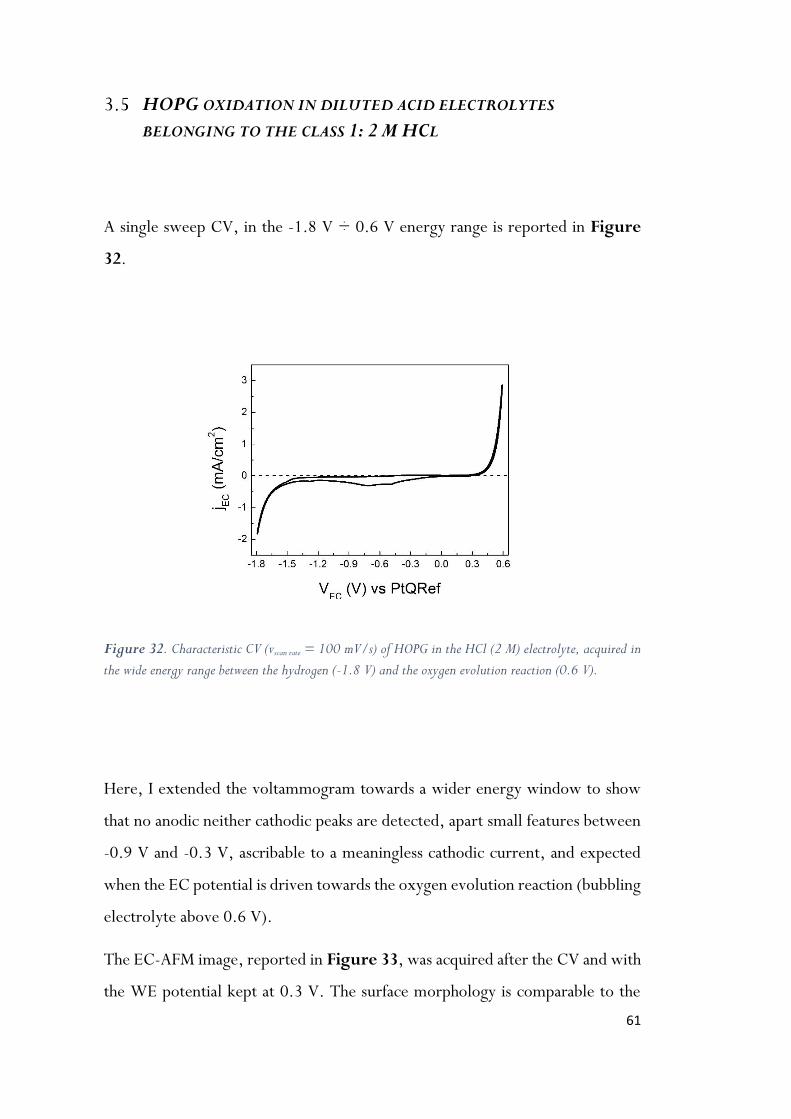
61

HOPG OXIDATION IN DILUTED ACID ELECTROLYTES

BELONGING TO THE CLASS 1: 2 M HCL

A single sweep CV, in the -1.8 V ÷ 0.6 V energy range is reported in Figure

32.

Figure 32. Characteristic CV (vscan rate = 100 mV/s) of HOPG in the HCl (2 M) electrolyte, acquired in

the wide energy range between the hydrogen (-1.8 V) and the oxygen evolution reaction (0.6 V).

Here, I extended the voltammogram towards a wider energy window to show

that no anodic neither cathodic peaks are detected, apart small features between

-0.9 V and -0.3 V, ascribable to a meaningless cathodic current, and expected

when the EC potential is driven towards the oxygen evolution reaction (bubbling

electrolyte above 0.6 V).

The EC-AFM image, reported in Figure 33, was acquired after the CV and with

the WE potential kept at 0.3 V. The surface morphology is comparable to the

62

topography observed on graphite simply immersed inside an electrolyte, where

no EC process was activated (see Figure 20). Sharp step edges, wide terraces, no

graphite basal plane swelling and a surface corrugation (along the dashed white

line) of about 0.1 nm characterize the image. Any carbon dissolution or blistering

process is visible and the whole morphology is in close agreement with pristine

HOPG (see Figure 18).

The HOPG stability in hydrochloric solution is also demonstrated by the EC-

STM structural analysis. The atomic-resolution image (see the inset of Figure 33)

shows the traditional graphite corrugation [(0.45 ± 0.08) Å] and no nano-

protrusion affects the STM image.

Figure 33. EC-AFM topography (5 x 5 m2) acquired on graphite immersed in 2 M HCl solution, after

a single CV sweep. Atomic resolution [EC-STM (5 x 5 nm2; Itunnel = 1 nA; Vbias = 0.3 V)] is reported in

the inset. At the bottom, scan profile of the graphite terraces along the white dashed line.

63

HOPG OXIDATION IN DILUTED ACID ELECTROLYTES:

DISCUSSION

In the light of the collected results, the comparison between class 2 and class 1

electrolytes demonstrates that nano-protrusion and surface blistering are

characteristic of sulfate and perchlorate anion intercalation. In particular, Figures

23 and 27 prove that nano-protrusions affect both blisters (or blister clusters)

and flat graphite surfaces, respectively.

I speculate that nano-protrusion can be thought in terms of an incipient blister,

which can growth and increase its sizes. Both nano-protrusions and blisters are

mechanically stable even when the WE is removed from the EC cell, suggesting

that the strained surface is equilibrated by an inner pressure (pint) of the HOPG

swelling. pint is produced after the oxidation of solvated anions inside the HOPG

crystal, but its value is difficult to calculate. Nano-protrusions look like nano-

bubbles produced by Ar [109], where the pint of some GPa is deduced from the

Ar trapped between graphene and Ir substrate.

Differently, in our case, three kind of gases are probably produced during

graphite oxidation (namely CO, CO2 and O2), whose relative amounts are

completely unknown. In addition, the volumetric size of nano-bubbles are well

defined, while nano-protrusions could extend inside the uppermost graphite

layer. Nonetheless, if I hypnotize that nano-protrusions (10 time smaller than

nano-bubbles in the exposed volume) are completely confined onto the HOPG

surface (single graphene layer), I can estimate in first approximation pint, by

considering the Young’s modulus for the graphene (ca 1 Tpa [115]) and the C-C

strein previously estimated by the geometrical construction. The so obtained

value of few GPa is in good agreement with the result for the Ar nano-bubbles

[109].

An estimation of pint is even more complex if blisters are taken into account,

where the number of graphite layers affected by the swelling is still unknown. In

64

addition, in this case, it is difficult to appreciate a C-C bond stretch from EC-

STM images. If blisters are considered, in a very first approximation, in the

framework of the Laplace law (mechanical equilibrium in bubbles):

𝑝𝑖𝑛𝑡 − 𝑝𝑒𝑥𝑡 ∝𝛾

𝑟

where the pext is approximated to the atmosphere, 𝛾 is the mean surface tension

for a graphene multilayer (0.1 J/m2) [116] and r = 350 nm (see the blister sizes

reported above), the resulting internal pressure consists of only few

atmospheres.

This rough estimation requires an experimental evidence as, for instance, stress-

strain analysis by EC-AFM. These measurements will be collected in the next

future. However, despite the simplicity of the used models, a decreasing pint from

nano-protrusion to blisters sustains the basic idea that the latter, with a pressure

close to pext, represent the final stage of the former growth. The coexistence of

nano-protrusion on blisters or clusters is beyond this simple mechanical model.

The nano-protrusion and blister evolution is in agreement with the interpretative

work in the literature [41]. Here, the authors suggest that step edges and surface

defects could be the preferential entrance of solvated anions. Figure 34 clearly

proves this hypothesis following the morphological evolution of the HOPG WE

immersed in HClO4 solution as a function of time. Keeping the EC potential in

the cell slightly lower than 0.9 V, in order to slow down the anion intercalation

rate, I observed that the graphite steps are quickly smoothed and the edges

eroded (see the black dashed squares in the figure). In particular, I found that

surface holes evolve, showing a progressive broadening within a few minutes

(dashed line), while other defects are formed, probably following the carbon

dissolution (dashed circles).

65

Figure 34. EC-STM images (Itunnel = 0.7 nA; Vbias = 0.8 V) acquired on graphite in HClO4 solution (2 M) at an

EC potential just below 0.9 V. The acquisition time of each image (panels a, b and c) is 150 s. The reported t

refers to the elapsed time computed from the scanning start of the first image (a) to the scanning start of the b) (150

s) or c) (300 s) image. The formation of damages (holes) on the graphite surface is marked by dashed circles. Pre-

existing damages increase their sizes (see the dashed straight line). In addition, I observe that the terrace edges are

smoothed and the corner eroded, as marked by the dashed squares.

Carbon dissolution, faceting, edges smoothing, nano-protrusions and blisters

represent a very critical phenomenology, because all of them participate to the

HOPG basal plane detriment, which limits size and quality of graphene flake

production. A stratagem to isolate each process from the others and shine a light

on the single molecular mechanism, is offered by the NPV (see Experimental

techniques).

66

H2SO4/HOPG SURFACE EVOLUTION ANALYZED BY NPV

The NPV analysis was used for studying the H2SO4 (1 M)/HOPG system. The

latter was chosen as a model case for the class 2 electrolytes, because the IV and

III intercalation stages are placed at well defined EC potentials (1.1 V and 1.2 V,

respectively) and the related traditional CV shows a high reproducibility. These

aspects help in defining the precise potential at which the pulse should be set to

induce a desired process.

Three EC potentials are chosen: 0.7 V, 1.0 V and 1.2 V, which are values

representative of the three faradaic current intervals observed in CV (see Figure

21). The pulse width minimum is = 0.2 s (-pulse), accordingly to the

discussion reported in the Experimental technique chapter.

After many preliminary tests, I observed that if an EC process (e.g. blistering)

affects the WE surface after N × -pulses (total time duration t = N) at a

defined VEC, blisters are also found if a single pulse of t = N seconds is applied

at the same EC potential. This means that only the total time interval t plays a

crucial role in the HOPG surface changes. The use of a minimum -pulse, which

can be repeated N times, helps in finding quickly the effective time of an EC

process at a defined VEC (e.g. blistering: tblister). The latter is defined as the

minimum time interval required to observe statistically blisters on the HOPG

surface, allowing a quantification of the process kinetics.

The WE, initially at VEC = 0.3 V, was set at 1.2 V for a time interval of 0.2 s (-

pulse, see Figure 35) and then reported at 0.3 V. After the pulse, the HOPG

surface was studied by the EC-STM, as reported in Figure 36.

67

Figure 35. Characteristic VEC vs time curve of a -pulse. Initial potential = 0.3 V; step potential = 1.2

V; duration = 0.2 s; sampling interval = 0.001 s.

68

Figure 36. EC-STM (500 x 500 nm2) images (Itunnel = 1.0 nA; Vbias = 0.3 V). a) image acquired at VEC

= 0.3 V after a pulse of 0.2 s at 1.2 V. The dashed black lines mark the edges of two terraces. b) image

acquired after about 60 s from the previous one (a). The terrace dissolution is clear from a direct comparison

of the edges with the black dashed lines. c) image acquired 120 s after the (a) image.

Progressive dissolution of terraces is observed as a function of time, which

continues for some minutes after the application of the -pulse, worsening the

quality of the HOPG basal plane even at 0.3 V. A statistical analysis on different

areas of the WE confirms the detriment of the sample.

Incidentally, I observe that no HOPG swellings or blisters are present on the

surface. This situation is unchanged after a second pulse of 2s (total t = 0.6

s) at 1.2 V, as demonstrated by Figure 37. Here, the dashed lines emphasize the

residuals of an original graphite terrace, which is almost completely dissolved.

Figure 37. EC-STM (300 × 300 nm2) image of HOPG surface after a second pulse of 0.4 s (total t = 0.6 s) at 1.2 V (Itunnel = 1 nA, Vbias = 0.3 V). The dashed black line emphasizes the residual of an original graphite terrace, which is almost completely dissolved.

69

When the total pulse time t is between 0.8 s and 1.6 s, blistering joins the

carbon dissolution process, as observed in Figure 38 (here, only part of a blister

is visible on the left-bottom corner of the image). These blisters show smaller

sizes (lateral width of only 100 nm and a height of about 5 nm) compared with

those acquired after a CV (see Figure 23). I interpret these incipient structures

as due to the first growth stages of those blisters that, keeping the sample at 1.2

V for a longer time, evolve in the huge structures reported and discussed above.

Figure 38. EC-STM (300 × 300 nm2) image of HOPG graphite after a total pulse of 1.6 s at 1.2 V

(Itunnel = 1 nA; Vbias = 0.3 V). The dashed black line emphasizes edge dissolution and HOPG swelling due

to a blister (left-bottom corner).

Blisters start to characterize statistically EC-STM images after a pulse of 1.6 s.

Consequently, I define tblister = 1.6 s as the effective time for surface blistering.

After a total interval time of 3.2 s at 1.2 V, the HOPG surface is completely

covered by blisters, as proved by Figure 39.

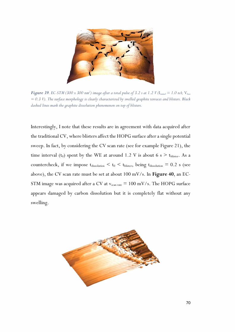
70

Figure 39. EC-STM (300 x 300 nm2) image after a total pulse of 3.2 s at 1.2 V (Itunnel = 1.0 nA; Vbias

= 0.3 V). The surface morphology is clearly characterized by swelled graphite terraces and blisters. Black

dashed lines mark the graphite dissolution phenomenon on top of blisters.

Interestingly, I note that these results are in agreement with data acquired after

the traditional CV, where blisters affect the HOPG surface after a single potential

sweep. In fact, by considering the CV scan rate (see for example Figure 21), the

time interval (t0) spent by the WE at around 1.2 V is about 6 s > tblister. As a

countercheck, if we impose tdissolution < t0 < tblister, being tdissolution = 0.2 s (see

above), the CV scan rate must be set at about 100 mV/s. In Figure 40, an EC-

STM image was acquired after a CV at vscan rate = 100 mV/s. The HOPG surface

appears damaged by carbon dissolution but it is completely flat without any

swelling.

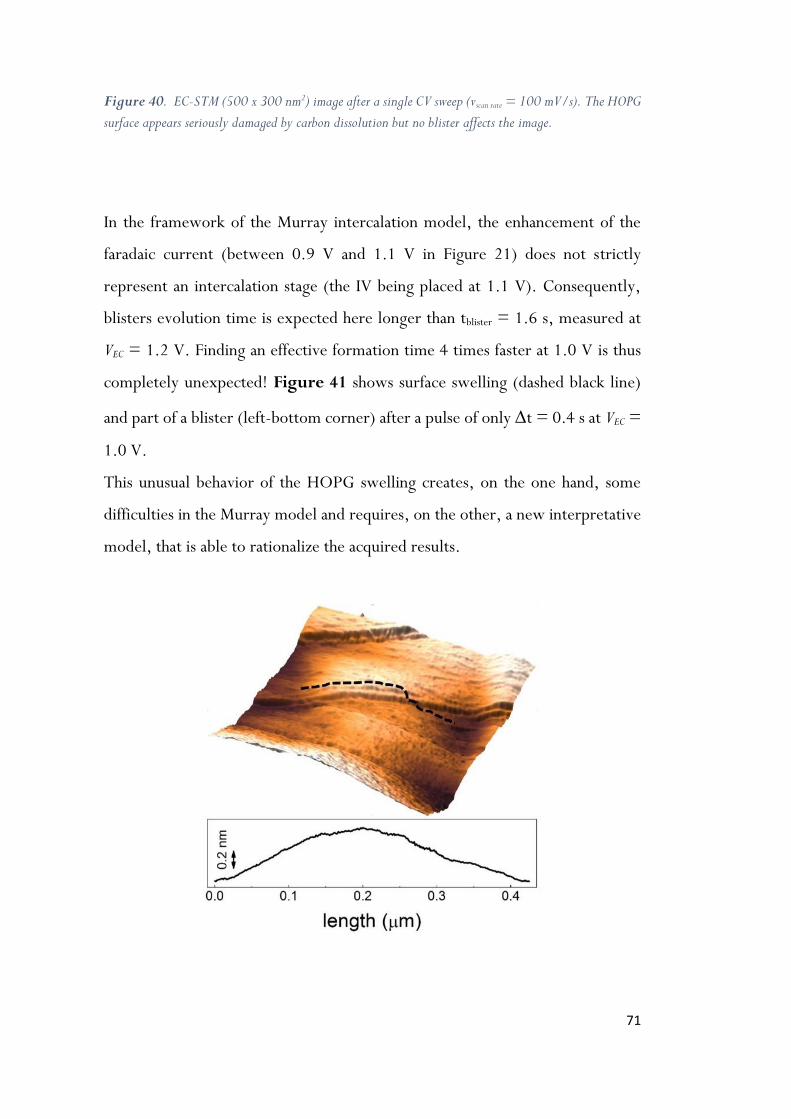
71

Figure 40. EC-STM (500 x 300 nm2) image after a single CV sweep (vscan rate = 100 mV/s). The HOPG

surface appears seriously damaged by carbon dissolution but no blister affects the image.

In the framework of the Murray intercalation model, the enhancement of the

faradaic current (between 0.9 V and 1.1 V in Figure 21) does not strictly

represent an intercalation stage (the IV being placed at 1.1 V). Consequently,

blisters evolution time is expected here longer than tblister = 1.6 s, measured at

VEC = 1.2 V. Finding an effective formation time 4 times faster at 1.0 V is thus

completely unexpected! Figure 41 shows surface swelling (dashed black line)

and part of a blister (left-bottom corner) after a pulse of only t = 0.4 s at VEC =

1.0 V.

This unusual behavior of the HOPG swelling creates, on the one hand, some

difficulties in the Murray model and requires, on the other, a new interpretative

model, that is able to rationalize the acquired results.

72

Figure 41. EC-STM (500 x 500 nm2) image after a total pulse of 0.4 s at 1.0 V (Itunnel = 1.0 nA; Vbias

= 0.3 V). The surface swelling is visible and its profile is reported at the bottom of the image. Part of a

blister is observed on the left-bottom corner of the image.

At this EC potential, HOPG is not affected by an intense carbon dissolution. Step

edges are sharp and terrace residuals are not observed in Figure 41. I also checked

that the graphite detriment is immaterial even for longer pulse intervals (not

reported here).

Finally, the H2SO4/HOPG system was analyzed by the NPV applied at 0.7 V.

Since at this potential no EC reactions occur on the WE, as measured by the

standard CV (null faradic current), no damages of the HOPG basal plane are

expected, regardless of the total pulse time used in NPV. As an example, Figure

42 reveals a regular flat HOPG surface after a total pulse of 1.6 s. Apart some

stripes, sometimes observed in diluted H2SO4 electrolyte by EC-SPM, the image

shows no carbon dissolution, swelling or blistering.

73

Figure 42. EC-STM (300 × 300 nm2) image acquired after a total pulse of 1.6 s at 0.7 V (Itunnel = 0.8

nA; Vbias = 0.3 V). The traditional graphite steps are visible and no damages are present. The profile

along the dashed black line is reported at the bottom.

74

H2SO4/HOPG SURFACE EVOLUTION ANALYZED BY NPV:

DISCUSSION

Results obtained by the NPV analysis are precious for the interpretation of the

anion intercalation mechanisms of the blistering process. Table 2 summarizes

the experimental data by reporting the effective times of the two main EC

processes observed by the EC-SPM investigation (carbon dissolution and surface

blistering).

EC process VEC = 0.7 V VEC = 1.0 V

(onset)

VEC = 1.2 V (III

stage)

carbon dissolution absent absent 0.2 s

surface blistering absent 0.4 s 1.6 s

Table 2. Rationale of the collected NPV data. The effective times of the observed EC processes are reported.

When the faradaic current is null in traditional CV (i.e. at 0.7 V), nor dissolution

neither blistering are observed in NPV. The HOPG WE is stable immersed in

diluted acid electrolytes and any surface delamination is possible.

The graphite surface undergoes a significant detriment when intercalation starts.

The above reported data are focused on the III stage, but no differences on the

effective times are observed when NPV is applied at 1.1 V (IV stage).

Interestingly, I found that tblister can be reduced of a significant percentage (not

more of 50%) if the pristine HOPG sample is particularly damaged by steps (e.g.

75

after hundreds of exfoliations by an adhesive tape), confirming that surface

defects are the main entrances of the solvated anions.

However, blisters take the order of few seconds (3.2 s in Figure 39) to cover the

HOPG surface. An interesting analysis was performed by Dimiev and co-workers

on the GIC formation time [117,118]. By an optical microscope investigation,

the authors show that the GIC effective time is of the order of tens of seconds.

On the other hand, Lee, Ahn and Ryu found that water intercalation in the

graphene/silica interface proceeds with a speed v = 3 m/h [119]. Assuming, in

a first approximation, the same v speed for solvated HSO4- anions during graphite

intercalation, tblisters corresponds to the required time interval to cross the very

first graphite bi-layers, suggesting that the sulfate oxidation and gas evolution are

almost instantaneous. Despite the interesting result, v speed is clearly

underestimated in this case, because the graphite defects (not taken into

consideration) further favor intercalation with the respect to the Lee and co-

workers system.

Following the Murray model, CO, CO2 and O2 molecules fill blisters. This

hypothesis is supported by the collected data. Carbon dissolution of the sample

surface is almost instantaneous at IV or III stage potential (see Figure 36). It is

reasonable to assume then, that dissolution also affects those inner graphite layers

joined by intercalated anions. In this case, in fact, the environment around an

inner or a surface carbon atom is comparable (see Figure 3 of the Introduction)

and similar processes are expected.

The described mechanisms involved during anion intercalation (first step of a

graphite delamination) represent an important drawback in graphene

production. The HOPG surface detriment continues for few minutes after a short

pulse (see Figure 36), damaging the graphene flakes and limiting the exploitable

area for applications. Each delamination procedure requires an intercalation

phase, the latter being always joined together with graphite dissolution.

76

An unexpected stratagem to overcome this bottleneck is offered by surface

blistering at lower EC potential (namely 1.0 V), where HOPG is not affected by

dissolution. Nonetheless, this result is difficult to rationalize in the Murray

framework. In fact, according to this model, anion intercalation is not expected

at EC potential below 1.1 V (IV stage).

I note that 1.0 V corresponds to the oxygen overpotential12 for an HOPG

electrode immersed in sulfuric acid electrolyte (see fig. 4 in Ref. 120). Oxygen

evolution in the inner cavities of graphite can reasonably swell the pristine HOPG

basal plane. If HSO4- is ruled out from intercalation, the hydroxyl group (OH-) is

the only electroactive species that can exchange charges at the WE, accordingly

to the following equation:

4𝑂𝐻− → 2𝐻2𝑂 + 𝑂2 + 4𝑒 −

This picture is confirmed by the CV (not reported here). If the WE undergoes a

single EC potential sweep up to 0.95 V, the voltammogram is almost flat and no

cathodic features (de-intercalation process) are observed. The latter appear as

soon as the EC potential reaches 1.0 V, suggesting that (OH-) intercalation starts.

Some EC-STM investigations at 1.0 V are currently underway.

Finally, when the WE is set to 1.2 V, hydroxyl groups intercalation is joined by

sulfate anions. The latter could cramp the process, delaying blistering from 0.4 s

to 1.6 s.

12 The overpotential is the difference between the electrode potential under the passage of a current and the thermodynamic value of the electrode potential in the absence of electrolysis.

77

4 CONCLUSION

Nowadays, 2-D electronics requires flat, flexible and resistant devices and

graphene has proved to be the proper material for electronics development. In

this respect, huge amount of high-quality graphene flakes are required for

electronic device commercialization and the EC graphite delamination represents

a concrete strategy to produce graphene. Intercalation of molecules inside the

stratified structure of HOPG reduces the layer-layer interaction, favoring the

graphite delamination. Despite the very good results obtained in terms of

graphene sheet sizes and quality, a significant percentage of flakes results

damaged and with a radius below 1 m. In view of a further improvement of

graphene production, research must focus on the molecular mechanisms of anion

intercalation and follow the surface evolution of the pristine HOPG crystal, when

immersed in diluted acid electrolytes. Unfortunately, the present interpretative

model of intercalation results insufficient in explaining the mechanisms, when

investigated at the nano-scale.

In this thesis, I propose a combined EC and SPM investigation applied to 2 classes

of acids (sulfuric and phosphoric, respectively), trying to overcome the

difficulties met by previous researches. In particular, the use of NPV revealed its

potentiality in discriminating different processes acting on the HOPG surface at

different EC potentials. In the Introduction of this work, I reported some open

questions that now, in the light of the collected data, can find an answer.

I unambiguously proved that step edges and surface defects are preferential

entrances for anions. The high EC potential, traditionally used for intercalation,

dissolves carbon and produces a significant detriment of the graphite basal plane,

limiting the quality of the graphene flakes produced. On the other hand, carbon

dissolution creates new defects and holes on the HOPG surface, which promote

anion intercalation.

78

Blistering affects the HOPG surface and shows a strained graphite structure that

reasonably relaxes after the graphite delamination, as supported by the literature

on graphene flakes. Blisters are stable and cover the electrode surface in few

seconds. Their stability is obtained by an equilibrium between the strained lattice

and the inner pressure. The latter is produced by CO, CO2, O2 molecules. In

particular, I gave full evidence that carbon dissolution can sustain the formation

of CO and CO2.

The overall picture of anion intercalation seems to be not challenging because

HOPG detriment significantly affects each intercalation stage, precluding a

further optimization of graphene production. The NPV analysis has disclosed

unexpected phenomena that could overcome the apparent bottleneck described

above. In fact, an intercalation process is observed at lower potentials, where

oxygen evolution starts but carbon dissolution is immaterial. This occurrence

was not considered within the traditional intercalation model. In this thesis work,

I proposed that hydroxyl groups intercalate inside the graphite, at lower EC

potential, favoring the surface swelling. When sulfate (or perchlorate) anions

start intercalation (IV and III stages), they indeed represent obstacles in the OH-

and HSO4- (or ClO4

-) co-intercalation and, as a consequence, the blistering time

formation is delayed.

Some perspectives of this research can be outlined.

Morphological and structural changes at oxygen overpotential regime are

currently in progress and require further investigations. In particular, being

hydroxyl groups present in all the used EC solutions, the blister effective time

should be the same if the oxygen overpotential onset is reached by the WE. This

constrain was realized during the sulfuric and perchloric analysis, but electrolytes

belonging to class 1 did not fulfill this requirement. In fact, phosphoric and

hydrochloric solutions show a faradaic current enhancement (compatible with an

incipient intercalation process, see Figures 29 and 32) but no cathodic features

79

(de-intercalation) are observed, suggesting that the EC analysis should be

extended towards higher potentials.

After blistering at 1.0 V, graphite delamination should be tested. This means that

the OH--intercalated graphite should be immersed in an ultra-sonic bath to

facilitate the graphene flake production. The latter could be then compared

(sizes, quality, timing, etc.) with flakes produced by the traditional protocol at

1.2 V.

A comparison between the mechanical properties of blisters (stress-strain curves)

produced at different EC potentials, is still missing; instead, it could clarify

differences between blisters filled by only O2 and those, where also CO and CO2

molecules are enclosed.

Finally, other electrolytes could be investigated in view of finding a better

compromise between anion intercalation and carbon dissolution.

80

5 REFERENCE

(1) Reddy, A.L.M.; Srivastava, A.; Gowda, S.R.; Gullapalli, H.; Dubey, M.;

Ajayan, P.M. Synthesis of nitrogen-doped graphene films for lithium battery application. ACS Nano 2010, 4(11), 6337–6342.

(2) Koehne, J.; Chen, H.; Li, J.; Cassell, A. M; Ye, Q.; Ng, H. T; Han, J.; Meyyappan, M. Ultrasensitive label-free DNA analysis using an electronic chip based on carbon nanotube nanoelectrode arrays. Nanotechnol. 2003, 14, 1239-1245.

(3) Besenhard, J.O.; Fritz, H.P. The electrochemistry of black carbons. Angew. Chem., Int. Ed. Engl. 1983, 22(12), 950–975.

(4) Crevillen, A.G.; Pumera, M.; Gonzalez, M.C.; Escarpa, A. The preferential electrocatalytic behaviour of graphite and multiwalled carbon nanotubes on enediol groups and their analytical implications in real domains. Analyst 2009, 134(4), 657–662.

(5) Saito, R.; Fujita, M.; Dresselhaus, G.; Dresselhaus, M.S. Electronic structure

of chiral graphene tubules. Appl. Phys. Lett. 1992, 60(18), 2204.

(6) Jouikov, V.; Simonet, J. Novel method for grafting alkyl chains onto glassy

carbon. Application to the easy immobilization of ferrocene used as redox probe.

Langmuir 2012, 28(1), 931–938.

(7) González Orive, A.; Grumelli, D.; Vericat, C.; Ramallo-López, J.M.;

Giovanetti, L.; Benitez, G.; Azcárate, J.C.; Corthey, G.; Fonticelli, M.H.;

Requejo, F.G.; Hernández Creus, A.; Salvarezza, R.C. ‘Naked’ gold nanoparticles

supported on HOPG: melanin functionalization and catalytic activity. Nanoscale

2011, 3(4), 1708–1716.

(8) Aoki, M.; Amawashi, H. Dependence of band structures on stacking and field

in layered graphene. Solid State Commun. 2007, 142, 123–127.

(9) Trucano, P.; Chen, R. Structure of graphite by neutron diffraction. Nature

1975, 258, 136.

(10) Bernal, J.D. The Structure of Graphite. Proc. R. Soc. London, Ser. A 1924, 106,

749–773.

(11) Alkire R. C.; Bartlett P. N.; Lipkowski J. Advances in Electrochemical

Science and Engineering Vol. 16, Wiley, New York (2015).

81

(12) Reich, S.; Thomsen, C. Raman spectroscopy of graphite. Philos. Trans. R. Soc.

London, Ser. A 2004, 362, 2271–2288.

(13) Data obtained from © Optigraph GmbH Web page.

(14) Spanu, L.; Sorella, S.; Galli, G. Nature and Strength of Interlayer Binding in

Graphite. Phys. Rev. Lett. 2009, 103, 196401.

(15) Lee, C.; Wei, X.; Kysar, J.W.; Hone, J. Measurement of the Elastic

Properties and Intrinsic Strength of Monolayer Graphene. Science 2008, 321, 385–

388.

(16) Tománek, D. and Louie, S.G. First-principles calculation of highly

asymmetric structure in scanning-tunneling-microscopy images of graphite. Phys.

Rev. B 1988, 37, 8327–8336.

(17) Jayasena, B.; Subbiah, S. A novel mechanical cleavage method for

synthesizing few-layer graphenes. Nano. Res. Lett. 2011, 6(95), 1-7.

(18) Lapshin, R.V. Automatic lateral calibration of tunneling microscope

scanners. Rev. Sci. Instrum. 1998, 69(9), 3268.

(19) Binnig, G.; Quate, C.F.; Gerber, C. Atomic Force Microscope. Phys. Rev.

Lett. 1986, 56, 930–933.

(20) McCreery, R.L. Carbon electrodes: structural effects on electron transfer

kinetics, in Electroanalytical Chemistry, vol. 17, Marcel Dekker, New York

(1991).

(21) McCreery, R.L. Advanced Carbon Electrode Materials for Molecular

Electrochemistry. Chem. Rev. 2008, 108, 2646–2687.

(22) Xia, J.; Chen, F.; Li, J.; Tao, N. Measurement of the quantum capacitance

of graphene. Nat. Nanotechnol. 2009, 4, 505–509.

(23) Zhong, J. H.; Liu, J. Y.; Li, Q.; Li, M. G.; Zeng, Z. C.; Hu, S.; Wu, D. Y.;

Cai, W.; Ren, B. Interfacial capacitance of graphene: Correlated differential

capacitance and in situ electrochemical Raman spectroscopy study. Electrochim.

Acta 2013, 110, 754–761.

(24) Rice, R.J.; Pontikos, N.M.; McCreery, R.L. Quantitative correlations of

heterogeneous electron-transfer kinetics with surface properties of glassy carbon

electrodes. J. Am. Chem. Soc. 1990, 112, 4617–4622.

82

(25) Cline, K.K.; McDermott, M.T.; McCreery, R.L. J. Anomalously Slow

Electron Transfer at Ordered Graphite Electrodes: Influence of Electronic Factors

and Reactive Sites. Phys. Chem. 1994, 98, 5314–5319.

(26) Brownson, D. A. C.; Banks, C. E. The Handbook of Graphene

Electrochemistry, Ch. 2, Springer, Berlin (2014).

(27) Dreyer, D. R.; Park, S.; Bielawski, C. W.; Ruoff, R. S. The chemistry of

graphene oxide. Chem. Soc. Rev. 2010, 39, 228.

(28) Shih, C. J. et al. Bi- and trilayer graphene solutions. Nat. Nanotechnol. 2011,

6, 439.

(29) Nicolosi, V.; Chhowalla, M.; Kanatzidis, M. G.; Strano, M.S.; Coleman, J.

N. Liquid Exfoliation of Layered Materials. Science 2013, 340, 1226419.

(30) Eda, G. et al. Photoluminescence from chemically exfoliated MoS2. Nano

Lett. 2011, 11, 5111.

(31) Xia, Z. Y. et al. The Exfoliation of Graphene in Liquids by Electrochemical,

Chemical, and Sonication-Assisted Techniques: A Nanoscale Study. Adv. Funct.

Mater. 2013, 23, 4684-4693.

(32) Qi, B.; He, L.; Bo, X.; Yang, H.; Guo, L. Electrochemical preparation of

free-standing few-layer graphene through oxidation–reduction cycling. Chem. Eng.

J. 2011, 171, 340-344.

(33) Kinoshita, K. Carbon. Electrochemical and Physicochemical Properties.

Wiley, New York (1988).

(34) Dresselhaus, M. S.; Endo, M. Graphite Intercalation Compounds II.

Springer, Berlin (1992).

(35) Zheng, T.; Reimers, J.N.; Dahn, J.R. Effect of turbostratic disorder in

graphitic carbon hosts on the intercalation of lithium. Phys. Rev. B 1995, 51(2),

734-741.

(36) Alliata, D. Investigation of Nanoscale intercalation into graphite and carbon

materials by in situ Scanning Probe Microscopy. PhD Thesis, Berna (2000).

(37) Singh, P. R.; Zeng X. Size-Dependent Intercalation of Ions into Highly

Oriented Pyrolytic Graphite in Ionic Liquids: An Electrochemical Atomic Force

Microscopy Study. J. Phys. Chem. C 2011, 115, 17429–17439.

83

(38) Beck, F.; Krohn H. Reversible Electrochemical Intercalation of Anions from

Aqueous Solutions in Polymer Bound Graphite Electrodes. Synth. Met. 1983, 7,

193 – 199.

(49) Goss, C. A.; Brumfield, J. C.; Irene, E. A.; Murray, R. W. Imaging the

Incipient Electrochemical Oxidation of Highly Oriented Pyrolytic Graphite. Anal.

Chem. 1993, 65, 1378−1389.

(40) Hathcock, K. W.; Brumfield, J. C.; Goss, C. A.; Irene, E. A.; Murray, R.

W. Incipient Electrochemical Oxidation of Highly Oriented Pyrolytic Graphite:

Correlation between Surface Blistering and Electrolyte Anion Intercalation. Anal.

Chem. 1995, 67, 2201 -2206.

(41) Alsmeyer, D.C.; McCreery, R.L. In Situ Raman Monitoring of

Electrochemical Graphite Intercalation and Lattice Damage in Mild Aqueous

Acids. Anal. Chem. 1992, 64, 1528–1533.

(42) Zhang, B.; Wang, E. Effects of Anodic Oxidation on the Surface Structure of

Highly Oriented Pyrolytic Graphite Revealed by In Situ Electrochemical Scanning

Tunneling Microscopy in H2SO4 Solution. Electrochim. Acta 1995, 40, 2627−2633.

(43) Schnydera, B.; Alliata, D.; Kötz, R.; Siegenthaler H. Electrochemical

intercalation of perchlorate ions in HOPG: an SFM/LFM and XPS study. Appl.

Surf. Sci. 2001, 173, 221-232.

(44) Bussetti, G.; Yivlialin, R.; Alliata, D.; Li Bassi, A.; Castiglioni, C.;

Tommasini, M.; Casari, C. S.; Passoni, M.; Biagioni, P.; Ciccacci, F.; Duo , L.

Disclosing the Early Stages of Electrochemical Anion Intercalation in Graphite by

a Combined Atomic Force Microscopy/Scanning Tunneling Microscopy

Approach. J. Phys. Chem. C 2016, 120, 6088−6093.

(45) Bard, A.J.; Faulkner, L. Electrochemical Methods. Wiley, New York

(2001).

(46) Bagotsky, V.S. Fundamentals of Electrochemistry. Wiley, New York (2005).

(47) Gulaboski, R.; Pereira C. M. Electroanalytical Techniques and

Instrumentation in Food Analysis. Handbook of Food Analysis Instruments, CRC

Press, Boca Raton (2009).

(48) Pyun, S. I.; Shin, H. C.; Lee, J. W.; Go, J. Y. Electrochemistry of Insertion

Materials for Hydrogen and Lithium. Springer, Berlin (2012).

(49) Kissinger, P. T.; Heineman, W. R. Cyclic Voltammetry. J. Chem. Educ. 1983,

60(9), 702.

84

(50) Brett, C. M. A.; Brett, A. M. O. Electrochemistry Principles, Methods, And

Applications. Oxford University Press, New York (1993).

(51) Reiss, H.; Heller, A. The Absolute Potential of the Standard Hydrogen

Electrode: A New Estimate J. Phys. Chem. 1985, 89, 4207-4213.

(52) Inzelt, G.; Lewenstam, A.; Scholz, F. Handbook of Reference Electrodes.

Springer, Berlin (2013).

(53) Fick A. On liquid diffusion. J. Membr. Sci. 1995, 100, 33-38.

(54) Kooijman, H. A. A Modification of the Stokes-Einstein Equation for

Diffusivities in Dilute Binary Mixtures. Ind. Eng. Chem. Res. 2002, 41, 3326-3328.

(55) Bauer, H. H.; Christian, G. D.; O’Reilly J. E. Analisi strumentale. Piccin

(1985).

(56) Beck, F.; Junge, H.; Krohn, H. Graphite Intercalation Compounds As

Positive Electrodes In Galvanic Cells. Electrochim. Acta 1981, 26, 799-809.

(57) Grahame, D. C. The Electrical Double Layer And The Theory Of

Electrocapillarity. Chem. Rev. 1947, 41(3), 441–501.

(58) Shahrokhian, S.; Asadian, E. Simultaneous voltammetric determination of

ascorbic acid, acetaminophen and isoniazid using thionine immobilized multi-

walled carbon nanotube modified carbon paste electrode. Electrochim. Acta 2010,

55, 666–672.

(59) Binnig, G.; Rohrer, H.; Gerber, C.; Weibel, E. Tunneling through a

Controllable Vacuum Gap. Appl. Phys. Lett. 1982, 40, 178-180.

(60) Binnig, G.; Rohrer, H.; Gerber, C.; Weibel, E. Surface Studies by Scanning

Tunneling Microscopy. Phys. Rev. Lett. 1982, 49, 57-61.

(61) Frommer, J. Scanning tunneling microscopy and atomic force microscopy in

organic chemistry. Angew. Chem. Int. Ed. 1992, 31, 1298-1328.

(62) Samori, P. Scanning probe microscopies beyond imaging. J. Mater. Chem.

2004, 14, 1353-1366.

(63) Kolb, D.M.; Simeone, F.C. Electrochemical nanostructuring with an STM:

A status report. Electrochim. Acta 2005, 50, 2989-2996.

(64) Bard, A.J.; Fan, F.R. Introductory lecture studies of the liquid-solid interface

by scanning-Tunneling-microscopy and scanning electrochemical microscopy.

Faraday Discuss. 1992, 94, 1-22.

85

(65) Sonnenfeld, R.; Hansma, P.K. Atomic-resolution microscopy in Water.

Science 1986, 232, 211-213.

(66) Hansma, P.K.; Tersoff, J. Scanning tunneling microscopy. J. Appl. Phys.

1987, 61, 1-23.

(67) Hansma, P.K.; Elings, V.B.; Marti, O.; Bracker, C.E. Scanning tunneling

microscopy and atomic force microscopy: Application to biology and technology.

Science 1988, 242, 209-216.

(68) Itaya, K.; Tomita, E. Scanning tunneling microscope for electrochemistry-A

new concept for the In situ scanning tunneling microscope in electrolyte solutions.

Surf. Sci. 1988, 201, 507-512.

(69) Itaya, K. In situ scanning tunneling microscopy in electrolyte solutions. Prog.

Surf. Sci. 1998, 58, 121-247.

(70) Wilms, M.; Kruft, M.; Bermes, G.; Wandelt, K. A new and sophisticated

electrochemical scanning tunneling microscope design for the investigation of

potentiodynamic processes. Rev. Sci. Instrum. 1999, 70, 3641-3650.

(71) Yagati, A. K.; Min, J.; Choi J.W. Electrochemical Scanning Tunneling

Microscopy (ECSTM) – From Theory to Future Applications. Modern

Electrochemical Methods in Nano, Surface and Corrosion Science, INTECH

(2014).

(72) Díez-Péreza, I.; Sanza, F.; Gorostizab, P. In situ studies of metal passive

films. Curr. Opin. Solid State Mater. Sci. 2006, 10, 144-152.

(73) Kabasakaloğlu, K.; Kiyak, T.; Sendil, O.; Asan, A. Electrochemical behavior

of brass in 0.1 M NaCl. Appl. Surf. Sci. 2002, 193(1-4) 167-174.

(74) Zamborni, F. P.; Crooks, R. M. Corrosion passivation of gold by n-

alkanethiol self-assembled monolayers:  Effect of chain length and end group.

Langmuir 1998, 14(12), 3279-3286.

(75) Hai, N.T.M.; Kosmala, T.; Wandelt, K. Potential dependence of self-

assembled porphyrin layers on a Cu(111) electrode surface: In-situ STM study.

Surf. Sci. 2015, 631, 207–212.

(76) Goletti, C.; Bussetti, G.; Violante, A.; Bonanni, B.; Di Giovannantonio, M.;

Serrano, G.; Breuer, S.; Gentz, K.; Wandelt, K. Cu(110) Surface in Hydrochloric

Acid Solution: Potential Dependent Chloride Adsorption and Surface

Restructuring. J. Phys. Chem. C 2015, 119, 1782−1790.

86

(77) Gittins, D. I.; Bethell, D.; Schiffrin, D. J.; Nichols R. J. A nanometre-scale

electronic switch consisting of a metal cluster and redox-address able groups.

Nature 2000, 408, 67-69.

(78) Kim S.U.; Yagati, A.K.; Min, J.; Choi, J.W. Nanoscale protein-based

memory device composed of recombinant azurin. Biomaterials 2010, 31(6), 1293-

1298.

(79) Artes, J.M; Diez-perez I; Sanz, F.; Gorostiza P. Direct measurement of

electron transfer distance decay constants of single redox proteins by

electrochemical tunneling spectroscopy. ACS Nano 2011, 5(3), 2060-2066.

(80) Tersoff, J.; Hamann, D. R. Theory and Application for the Scanning

Tunneling Microscope. Phys. Rev. Lett. 1983, 50(25), 1998-2001.

(81) Oura K.; Lifshits V.; Saranin A.; Zotov A.; Katayama M. Surface Science An

introduction, Springer, Berlin (2003).

(82) Hallmark, V.M; Chiang, S.; Rabolt, J.F.; Swalen, J.D.; Wilson, R.J.

Observation of Atomic Corrugation on Au(111) by Scanning Tunneling

Microscopy. Phys. Rev. Lett. 1987, 59, 2879-2882.

(83) Auwärter, W.; Seufert, K.; Bischoff, F.; Ecija, D.; Vijayaraghavan, S.; Joshi,

S.; Klappenberger, F.; Samudrala, N.; Barth, J. V. A surface-anchored molecular

four-level conductance switch based on single proton transfer. Nature

Nanotechnology 2012, 7, 41-47.

(84) Tersoff, J.; Hamann. Theory of scanning tunneling microscope. Phys. Rev. B

1985, 31, 805-813.

(85) Hla, S.W. Scanning tunneling microscopy single atom/molecule

manipulation and its application to nanoscience and technology. J. Vac. Sci. Technol.

B 2005, 23, 1351-1360.

(86) Meyer, G.; Amer, N. M. Novel optical approach to atomic force microscopy.

Appl. Phys. Lett. 1988, 53, 1045-1047.

(87) Pethica, J. B.; Oliver, W. C. Tip Surface Interactions in STM and AFM.

Physica Scripta. 1987, T19, 61-66.

(88) Kouzeki, T.; Tatezono, S.; Yanagi, H. Electrochromism of Orientation-

Controlled Naphthalocyanine Thin Films. J. Phys. Chem. 1996, 100, 20097-20102.

(89) Manne, S.; Gaub, H. E. Molecular organization of surfactants at solid-liquid

interfaces. Science 1995, 270.5241, 1480.

87

(90) Roiter, Y.; Minko, S. AFM Single Molecule Experiments at the

Solid−Liquid Interface:  In Situ Conformation of Adsorbed Flexible

Polyelectrolyte Chains. J. Am. Chem. Soc. 2005, 127 (45), 15688–15689.

(91) Henderson, E.; Haydon, P. G.; Sakaguchi, D. S. Actin filament dynamics in

living glial cells imaged by atomic force microscopy. Science 1992, 257, 1944-

1946.

(92) Radmacher, M. Measuring the elastic properties of biological samples with

the AFM. IEEE Engineering in Medicine and Biology Magazine 1997, 16, 47-57.

(93) Lennard-Jones, J. E. Cohesion. Proc. Phys. Soc. 1931, 43, 461-482.

(94) Cappella, B.; Dietler G. Force-distance curves by atomic force microscopy.

Surf. Sci. Rep. 1999, 34, 1-104.

(95) Bradley, R.S. The Cohesive Force between Solid Surfaces and the Surface

Energy of Solids. Phil. Mag. 1932, 13, 853-862.

(96) Derjaguin, B. V.; Muller, V. M.; Toporov, Y. P. Effect of contact

deformations on the adhesion of particles. J. Colloid Interface Sci. 1975, 53, 314-

326.

(97) Johnson, K. L.; Kendall, K.; Roberts, A. D. Surface Energy and the Contact

of Elastic Solids. Proc. Roy. Soc. A 1971, 324, 301-313.

(98) Giessibl, F. J. Advances in atomic force microscopy. Rev. Mod. Phys. 2003,

75, 949-983.

(99) Teflon PTFE – fluoropolymer resin. Properties handbook, DuPont.

(100) Skoog, D. A.; Holler, J. F.; Crouch S. R. Chimica analitica strumentale,

Edises (2009)

(101) Alliata, D.; Kotz, R.; Haas, O.; Siegenthaler, H. In-Situ AFM Study of

Interlayer Spacing during Anion Intercalation into HOPG in Aqueous Electrolyte.

Langmuir 1999, 15, 8483−8489.

(102) Liu, J. et al. A green approach to the synthesis of high-quality graphene

oxide flakes via electrochemical exfoliation of pencil core. RSC Adv. 2013, 3,

11745–11750.

(103) Nyamjav, D. The Stm Imaging of The Surface Structure of Graphite.

(104) Nicholson, R. S. Theory and Application of Cyclic Voltammetry for

Measurement of Electrode Reaction Kinetics. Anal. Chem. 1965, 37 (11), 1351–

1355.

88

(105) Mabboil, G. A. An Introduction to Cyclic Voltammetry. J. Chem. Educ.

1983, 60(9), 697-702.

(106) Meyer, J. C.; Geim, A. K.; Katsnelson, M. I.; Novoselov, K. S.; Booth, T.

J.; Roth, S. The Structure of Suspended Graphene Sheets. Nature 2007, 446,

60−63.

(107) Fasolino, A.; Los, J. H.; Katsnelson, M. I. Intrinsic ripples in graphene. Nat.

Mater. 2007, 6, 858−861.

(108) Grantab, R.; Shenoy, V. B.; Ruoff, R. S. Anomalous Strength

Characteristics of Tilt Grain Boundaries in Graphene. Science 2010, 330,

946−948.

(109) Zamborlini, G.; Imam, M.; Patera, L. L.; Mentes, T. O.; Stojic , N.; Africh,

C.; Sala, A.; Binggeli, N.; Comelli, G.; Locatelli, A. Nanobubbles at GPa under

Graphene. Nano Lett. 2015, 15, 6162− 6169.

(110) Rong, Z. Y.; Kuiper, P. Electronic efFects in scanning tunneling

microscopy: Moire pattern on a graphite surface. Phys. Rev. B 1993, 48, 17427-

17431.

(111) Guenbour, A.; Iken, H.; Kebkab, N.; Bellaouchou, A.; Boulif, R.; Ben

Bachir, A. Corrosion of graphite in industrial phosphoric acid. Appl. Surf. Sci. 2006,

252, 8710–8715.

(112) Thiele, H. The oxidation of carbon in electrolytes at normal temperature.

Trans. Faraday Soc. 1938, 34, 1033-1039.

(113) Yivlialin, R.; Brambilla, L.; Bussetti, G.; Tommasini, M.; Li Bassi, A.;

Casari, C. S.; Passoni, M.; Ciccacci, F.; Duò, L.; Castiglioni, C. Evolution of the

graphite surface in phosphoric acid: an AFM and Raman study. Beilstein J.

Nanotechnol. 2016, 7, 1878–1884.

(114) Bartoli, A.; Papasogli, G. Sviluppo di eletricità per l'ossidazione a

freddo del carbone. Il Nuovo Cimento 1882, 10, 274-277.

(115) Lee, C.; Wei, X.; Kysar, J. W.; Hone, J. Measurement of the

Elastic Properties and Intrinsic Strength of Monolayer Graphene. Science

2008, 321, 384-388.

(116) Shih, C.J.; Strano, M. S.; Blankschtein D. Wetting translucency

of Graphene. Nature Mat. 2013, 12, 866-869.

89

(117) Dimiev, A. M. et al. Direct Real-Time Monitoring of Stage

Transitions in Graphite Intercalation Compounds. ACS Nano 2013, 7,

2773-2780.

(118) Dimiev, A. M.; Tour, J. M. Mechanism of Graphene Oxide

Formation. ACS Nano 2014, 8, 3060-3068.

(119) Lee, DE.; Ahn, G.; Ryu, S. Two-Dimensional Water Diffusion

at a Graphene–Silica Interface. J. Am. Chem. Soc. 2014, 136, 6634-6642.

(120) Tanaka, Y.; Furuta, M.; Kuriyama, K.; Kuwabara, R.; Katsuki, Y.; Kondo, T.; Fujishima, A.; Honda, K. Electrochemical Properties of N-Doped Hydrogenated Amorphous Carbon Films Fabricated by Plasma-Enhanced Chemical Vapor Deposition Methods. Electrochim. Acta 2011, 56, 1172-1181.