p-hacking:

Evidence from two million trading strategies

Tarun Chordia Amit Goyal Alessio Saretto∗

August 2017

Abstract

We implement a data mining approach to generate about 2.1 million trading strate-gies. This large set of strategies serves as a laboratory to evaluate the seriousness ofp-hacking and data snooping in finance. We apply multiple hypothesis testing tech-niques that account for cross-correlations in signals and returns to produce t-statisticthresholds that control the proportion of false discoveries. We find that the differencein rejections rates produced by single and multiple hypothesis testing is such that mostrejections of the null of no outperformance under single hypothesis testing are likelyfalse (i.e., we find a very high rate of type I errors). Combining statistical criteriawith economic considerations, we find that a remarkably small number of strategiessurvive our thorough vetting procedure. Even these surviving strategies have no the-oretical underpinnings. Overall, p-hacking is a serious problem and, correcting for it,outperforming trading strategies are rare.

∗Tarun Chordia is from Emory University, Amit Goyal is from Swisss Finance Institute at the Universityof Lausanne, and Alessio Saretto is from University of Texas at Dallas. We thank Campbell Harvey, OlivierScaillet and, especially, Michael Wolf for helpful discussions. All errors are our own.

An increasingly large body of literature studies the profitability of trading strategies

based on signals obtained from publicly available information. Researchers are currently

tracking a number of strategies well in excess of 300 and new papers keep adding to that

list.1

In his presidential address, Harvey (2017) questions whether the performance of these

strategies is real or apparent due to a number of possible problems with the way in which

these strategies are discovered. For example, the manner in which they are evaluated does

not align with the actual research process: many strategies are investigated, but only those

that are significant are reported as only they have a viable path to publication. Thus, data

snooping likely leads to a number of false rejections of the null. Also, a number of data

choices, test procedures, and samples may be tried until a significant result is discovered and

only the significant result is reported. He refers to all of that as p-hacking.

Professor Harvey is not alone. Other papers have studied out-of-sample performance of

popular trading strategies: Chordia, Subrahmanyam, and Tong (2014) document a decline in

the anomaly-based trading strategy profits over time. McLean and Pontiff (2015) show that

the performance of trading strategies declines after the publication of research papers that

document their discovery. Linnainmaa and Roberts (2016) consider the performance of a

few popular strategies in the period before and after the one that is studied in the paper that

claims discovery, and find that the out-of-sample performance is substantially weaker. Other

studies have resorted to replication exercises to confirm the validity of previous findings.

For example, Hou, Xue, and Zhang (2017) conduct a large-scale replication study of 447

anomalies and find that 65% are insignificant at the 5% level using conventional critical

values and 85% are insignificant using a critical value of three.

We take a comprehensive approach and propose a relative evaluation of all information

contained in the most commonly used finance datasets. In particular, we compute the

performance of a large number of trading strategies that encompass the majority of ways

in which public information from prices and balance sheets is currently used to construct

trading signals. We consider the list of all accounting variables on Compustat and basic

market variables on CRSP. We construct trading signals by considering various combinations

of these basic variables and construct roughly 2.1 million different trading signals. Since

we are not interested in promoting any particular strategy, the reader should think of our

exercise not as a fishing expedition to find new strategies but as a thorough use of the data

to properly evaluate an hypothesis, which Leamer (1978) refers to as data-mining.

We use such a large sample as a laboratory experiment to address two questions. First,

1For example, Harvey, Liu, and Zhu (2015) document the existence of 316 factors, Green, Hand, andZhang (2013) study over 300 strategies, and Hou, Xue, and Zhang (2017) study 447.

1

can we put a bound on the magnitude of p-hacking? Second, after accounting for p-hacking,

how likely is a researcher to find a truly abnormal trading strategy? There are two essential

features of our study that enable us to answer these questions.

First is our procedure for generating trading signals. Our strategy yields a comprehensive

set of trading strategies, some of which have been studied and published as well as some

that have been studied but not published (likely because they do not surpass traditionally

accepted statistical hurdles), and those that have yet to be studied (likely because their

economic foundation is not immediately justifiable or simply because researchers have not

thought about them). By accepting into the sample study strategies without filtering on their

ex-post significance, and/or by not relying on published anomalies, our large-scale exercise

allows us to avoid p-hacking and data snooping. Moreover, although all our results are robust

to various sample definitions, in order to mitigate concerns about economic robustness (Novy-

Marx and Velikov (2016) and Hou, Xue, and Zhang (2017)), we exclude stocks that have

prices below three dollars and market capitalization below the twentieth percentile of the

NYSE distribution (i.e., microcaps).

The second essential aspect of our study is that we rely on multiple hypothesis testing

(MHT) to control the proportion of false discoveries. When studying the entire distribution

of trading strategies, one has to account for the fact that some strategies’ performance will

appear exceptional by luck, thus leading to some false rejections of the null hypothesis of

no outperformance. The rate of false discovery increases with the number of strategies

considered, even when the strategies are completely independent. For instance, while a

significance level of 5% implies that Type I error (probability of false rejection) is 5% in

testing one strategy, the rate of Type I error (i.e., the probability of making at least one

false discovery) in testing ten (independent) strategies is 1− 0.9510 = 40%.

MHT has been recently examined by Harvey and Liu (2014, 2015) and Harvey, Liu, and

Zhu (2015). We follow their lead and rely on formal MHT to evaluate our very large cross-

section of strategies. The statistics and economics literature has proposed a variety of ways

for controlling the Type I error in testing multiple hypotheses. We consider the three most

common approaches: family-wise error rate (FWER), false discovery ratio (FDR), and false

discovery proportion (FDP). FWER controls for the probability of making even one false

rejection, FDP controls for probability of a user-specified proportion of false rejections in

a given sample, while FDR controls expected (across different samples) proportion of false

rejections.

Besides the conceptual distinction in what they are trying to control, these methods

also differ in their underlying assumptions. For our purposes, the most important of these

assumptions is that of independent strategies. Trading strategies are not independent of

2

each other, as there is cross-correlation in stock returns across different firms and in the

information used to construct the signals, not only across different firms but also within a

particular firm (i.e., total assets and profitability are not independent). Since FDP methods

deliver statistical cutoffs that rely on the cross-correlations present in the data, we rely on

these methods more heavily by implementing a bootstrap method similar to the one used in

Harvey and Liu (2016).

We calculate two measures of risk-adjusted performance for each of our strategy. First,

we construct a long-short portfolio based on the top and bottom decile of each signal’s

distribution. We then compute portfolio alphas using the Fama and French (2015) five factor

model augmented with the Carhart (1997) momentum factor. Second, we calculate the Fama

and MacBeth (1973), henceforth FM, coefficient for each signal following the methodology

proposed by Brennan, Chordia, and Subrahmanyam (1998).

Imposing a tolerance of 5% of false discoveries (false discovery proportion) and a signifi-

cance level of 5%, we find that the critical value for alpha t-statistic (tα) is 3.79 while that for

FM coefficient t-statistic (tλ) is 3.12. While these critical values are, obviously, quite a bit

higher than the conventional levels, they are not far from the suggestion of Harvey, Liu, and

Zhu (2015) to use a critical value of three. Our higher threshold is due to our choice of the

MHT methods, our sample of over two million strategies vis-a-vis slightly over 300 strategies

in Harvey, Liu, and Zhu, and the fact that we fully account for dependence in the data. At

these thresholds, 2.76% of strategies have significant alphas and 10.80% have significant FM

coefficients. The larger critical values for tλ than those for tα are due to the fact that the

cross-strategy distribution of the former has longer tails (i.e., the standard deviation of the

distribution of tλ is equal to 1.93, while the standard deviation of tα is 1.82).

Comparing the rejection rates obtained from MHT to the rejection rates obtained from

classical single hypothesis testing (CHT), which rejects any hypothesis with a t-statistic

higher than 1.96, gives a lower bound for the magnitude of p-hacking. Under CHT we

reject the null hypothesis in about 30% of the cases for both alpha and FM coefficient t-

statistics. That figure does not materially change if we apply a threshold p-value obtained

from the bootstrap methods of Kosowski, Timmermann, Wermers, and White (2006), Fama

and French (2010), and Yan and Zheng (2017), that control for cross-correlation in the data.

We conclude that the great majority of the discoveries (i.e., rejections of the null of no

predictability) that are made by relying on CHT and without accounting for the very large

number of strategies that are never made public, are very likely false. In the case of alphas,

that percentage can be as big as 91%, while the problem is less severe for FM coefficients,

although the upper bound might be still be 65% for the latter.

Up to this point we have exclusively relied on statistical considerations in conducting our

3

analysis. However, Harvey (2017) warns us that a more integrated approach is necessary

to reach robust conclusions about financial research. Therefore, we include some economic

considerations in our null rejection procedure.

In order to gauge economic significance, we impose two additional hurdles on strategies

that survive statistical thresholds. First, we impose consistency between performance mea-

sures obtained by portfolio sorts and those derived from FM regressions. The long-short

portfolio alphas effectively consider the efficacy of the strategy in only 20% of the sample

while FM regressions consider the entire sample. On the other hand, FM regressions impose

linearity while portfolio sorting allow for any functional relationship between signals and

returns in the data. There are, thus, advantages and disadvantages to both portfolio sorts

and regressions (Fama and French (2010)). Therefore we ask of a trading signal to not only

generate a high long-short portfolio alpha but also to explain the broader cross-section of

returns in a regression setting. Eliminating strategies that have statistically significant tα

but insignificant tλ, or vice-versa, drastically reduces the number of successful strategies to

806 (i.e., 0.04% of the total) under MHT and to 33,881 (i.e., 1.62% of the total) under CHT.

The second restriction that we impose is related to economic magnitudes. Because they

have a large tα, the surviving strategies also have large risk-adjusted abnormal returns.

However, we decide not to construct an alpha-based hurdle for two reasons: any threshold

of alpha would be largely subjective, and alphas do not reflect the actual trading profits

realized by the strategy. We opt instead to construct economic hurdles based on the Sharpe

ratio. The choice of the Sharpe ratio is motivated by two reasons. First, it reflects the

industry practice of investors. Second, it is easily comparable to largely held benchmark

portfolios such as the S&P 500 index or the value-weighted market portfolio. In short, we

eliminate strategies that do not have a Sharpe ratio higher than that of the value-weighted

market portfolio.

Imposing the two economic hurdles leaves us with 17 strategies (out of about 2.1 million)

that are both statistically and economically significant under MHT and 801 under CHT.

Following Harvey (2017), we also construct minimum Bayes factors and calculate bayesian

p-values. Restricting to the sample of 17 strategies that survive MHT and economic hurdles,

we find that, for a prior odds ratio of 99 to 1 indicating a very high degree of prior probability

of the null being true (what Harvey refers to as long shots),2 none of the strategies have

posterior p-values lower than 0.05 for both the alphas and the FM coefficients. With a prior

odds ratio of 90 to 10, nine of seventeen strategies have posterior p-values lower than 0.05

for both the alphas and the FM coefficients.

The statistical evidence, frequentist and Bayesian, coupled with economic constraints

2Given that our strategies have no theoretical basis, a long shot prior is appropriate.

4

thus still leads to a handful of strategies that present exceptional investment opportunities.

In other words, if our strategy construction and database choices are representative of the

larger universe of all possible strategies that can be constructed using all available datasets,

the likelihood of a researcher finding a truly abnormal trading strategy are incredibly low.

A closer inspection of the signals that generate the 17 surviving strategies leaves us with

some hesitation due to ostensible lack of any economic underpinnings. None of the remaining

set of strategies bears any relation to the set of published anomalies (using Hou, Xue, and

Zhang (2017) as a guide). For example, one of the strategies that survives is produced by

sorting stocks on the ratio of the difference between Total Other Liabilities and the value of

Property Sales to the Number of Common Shares. It seems hard to imagine a theoretical

model that would lead to predictions relying on this variable — statistical significance (even

with economic constraints) does not guarantee an economically plausible explanation. We

conclude that, despite almost half a century after Fama (1970), much work devoted to the

topic, innumerable new statistical techniques and economic models, a switch of accent from

stock returns to long-short portfolios, the standard of market efficiency is as strong as ever.

Our paper echoes the increasing skepticism about the validity of many research findings

in a variety of fields. While the findings on the lack of replicability in medical research by

Ioannidis (2005) are widely cited, the economics profession has also made an effort to tackle

this problem. Leamer (1978) famously complains about specification searches in empirical

research and proposes (1983) to take the ‘con’ out of econometrics. Dewald, Thursby, and

Anderson (1986), McCullogh and Vinod (2003), and Chang and Li (2017) also report dis-

appointing results from replication of economics papers. The use of replication in finance is

less widespread with Hou, Xue, and Zhang (2017) being a notable recent exception.

Our paper also joins the list of the growing finance literature that studies the prolifera-

tion of discoveries of abnormally profitable trading strategies and/or pricing factors and its

relation to data-snooping biases in finance. See Lo and MacKinlay (1990) and MacKinlay

(1995) for early work emphasizing statistical biases in hypothesis testing. The question of

whether the profitability of published strategies survives the test of time is studied in Schwert

(2003), Chordia, Subrahmanyam, and Tong (2014), McLean and Pontiff (2015), Linnainmaa

and Roberts (2016), and Hou, Xue, and Zhang (2017). Towards the turn of the century,

more formal statistical approaches were developed and applied to the problem of evaluat-

ing multiple strategies (see, for example, Sullivan, Timmermann, and White (1999), White

(2000), and Romano and Wolf (2005)). The MHT approach has been more recently applied

to financial settings in Barras, Scaillet, and Wermers (2010), Harvey, Liu, and Zhu (2015),

and emphasized in the presidential address of Harvey (2017). Our paper is also closely re-

lated to Yan and Zheng (2017). Both paper share the goal of evaluating a broader universe

5

of strategies than just the published ones. Beyond inevitable differences in sample construc-

tion etc., our conclusions about market efficiency differ markedly from theirs for two main

reasons. One is our use of formal statistical approaches to MHT rather than heuristic-based

bootstrapped approach. Second is our insistence on economic significance.

1 Data and trading strategies

Monthly returns and prices are obtained from CRSP. Annual accounting data come from

the merged CRSP/COMPUSTAT files. We collect all items included in the balance sheet,

the income statement, the cash-flow statement, and other miscellaneous items for the years

1972 to 2015. We choose 1972 as the beginning of our sample as it corresponds to the first

year of trading on Nasdaq that dramatically increased the number of stocks in the CRSP

dataset. All our results are robust to beginning the sample in 1963, which is the first date

on which the COMPUSTAT data are not affected by backfilling bias. Following convention,

we set a six-month lag between the end of the fiscal year and the availability of accounting

information.

We impose several filters on the data to obtain our basic sample. First, we include only

common stocks with CRSP share codes of 10 or 11. Second, we require that data for each

variable be available for at least 300 firms each month for at least 30 years during the sample

period. Third, in FM (1973) regressions described later, we require that data be available

for all independent variables (including the variable of interest) for at least 300 firms each

month for at least 30 years during the sample period. Fourth, at portfolio formation at the

end of June of each year (exact procedure described later), we require stocks to have a price

higher than three dollars and market capitalization to be higher than the bottom twentieth

percent of the NYSE capitalization. The last filter ensures that we eliminate micro-cap stocks

alleviating concerns about transaction costs (Novy-Marx and Velikov (2016) and Hou, Xue,

and Zhang (2017)).

There are 156 variables that clear our filters and can be used to develop trading signals.

The list of these variables is provided in Appendix Table A1. We refer to these variables

as Levels. We also construct Growth rates from one year to the next for these variables.

Since it is common in the literature to construct ratios of different variables we also compute

all possible combinations of ratios of two levels, denoted Ratios of two, and ratios of any

two growth rates, denoted Ratios of growth rates. Finally, we also compute all possible

combinations that can be expressed as a ratio between the difference of two variables to a

third variable (i.e., (x1 − x2)/x3). We refer to this last group as Ratios of three. We obtain

a total of 2,090,365 possible signals.

6

We evaluate trading signals by estimating abnormal performance of the hedge portfolios

using a factor model and by evaluating the ability of the signal in explaining the cross-section

of firms’ abnormal returns.

1.1 Hedge portfolios

We sort firms into value-weighted deciles on June 30 of each year and rebalance these portfo-

lios annually. The first portfolio formation is June 1973 and the last formation date is June

2015. We require a minimum of 30 stocks in each decile (300 stocks in total) in a month

to consider that month as having a valid return. The signal is considered to have generated

a valid portfolio if there are at least 360 months of valid returns. We consider long-short

portfolios only. Thus, we compute a hedge portfolio return that is long in decile ten and

short in decile one. Since we do not know ex-ante which of the two extreme portfolios has

the largest average return, our hedge portfolios can have either positive or negative average

returns. Obviously, it is always possible to obtain a positive average return for a hedge port-

folio that has a negative average return by taking the opposite positions. For expositional

convenience, we decide not to force average returns to be positive.

Our benchmark evaluation factor model is composed of the five factors in Fama and

French (2015) plus the momentum factor. The five factors are the market, size, value, in-

vestment, and profitability factors. For each trading strategy, we run a time-series regression

of the corresponding hedge portfolio returns on the six factors and obtain the alpha as well

as its heteroskedasticty-adjusted t-statistic, tα.

1.2 Fama-MacBeth regressions

Given that the alphas of the long-short portfolio effectively consider the efficacy of the

strategy in only 20% of the sample, we also evaluate a signal’s ability to predict returns in

the cross-section of stocks using FM (1973) regressions. In particular, we evaluate the ability

of the signal to explain stock returns by estimating the following cross-sectional regression

each month:

Rit − βiFt = λ0t + λ1tXit−1 + λ2tZit−1 + eit, (1)

where X is the variable that represents the signal and Z’s are control variables. We use the

most commonly used control variables, namely size (i.e., the natural logarithm of the firm’s

market capitalization), natural logarithm of the book-to-market ratio, past one-month and

11-month return (skipping the most recent month), asset growth, and profitability ratio.

Book-to-market is calculated following Fama and French (1992) while asset growth and

7

profitability are calculated following Fama and French (2015). We risk-adjust the returns on

the left-hand-side of equation (1) following Brennan, Chordia, and Subrahmanyam (1998).

We use the same six-factor model used to calculate hedge portfolio alphas, and calculate full-

sample betas β for each stock. We require at least 60 months of valid returns to estimate

the time-series regression.

In estimating the cross-sectional regressions, we require a minimum of 300 stocks in a

month. Finally, we require a minimum of 360 valid monthly cross-sectional estimates during

the sample period to calculate a valid λ1 coefficient for a signal. Thus, we calculate the FM

coefficient λ1 as well its heteroskedasticty-adjusted t-statistic (tλ). Given that we require a

valid beta for each stock and data on additional control variables, the data requirements for

regressions are slightly more stringent than those for portfolio formation.

2 Strategy performance

In this section we discuss the statistical properties of the signals and the trading strategy

returns. We analyze raw returns and Sharpe ratios in Section 2.1, and abnormal returns and

regression coefficients in Section 2.2 and 2.3.

2.1 Raw returns and Sharpe ratios

Table 1 reports summary statistics of raw returns on the hedge portfolios. We report cross-

sectional means, medians, standard deviation, minimum, and maximum across portfolios.

These statistics are reported for the sample of all portfolios as well as the sub-sample of

portfolios formed by the different trading signals (i.e., ratio of two, ratio of three, etc.). We

report monthly average returns in Panel A, t-statistics for returns in Panel B, and monthly

Sharpe ratios in Panel C. Each panel also reports the number and percentage of portfolios

that cross specific thresholds.

Panel A shows that the cross-sectional mean and median average return of the portfolios

are close to zero. The cross-sectional standard deviation of returns at 0.18% coupled with

the fact that we have over two million portfolios implies that there are many portfolios

with very large absolute returns. For example, there are 17,192 portfolios with absolute

average monthly return greater than 0.5%. Panel B shows that a large number of portfolios

have average returns that exceed conventional statistical significance levels. 22,237 portfolios

have average return t-statistics larger than 2.57 (in absolute value); albeit this represents only

about 1% of the total number of portfolios. The economic importance of these portfolios is

also very impressive as many portfolios have monthly Sharpe ratios higher than the historical

8

market Sharpe ratio (approximately 0.116), with one portfolio having a Sharpe ratio higher

than 0.232. These facts, while not perhaps surprising, are, nevertheless, interesting because

they are obtained despite the stringent rules that affect the composition of our universe of

stocks and signals (e.g., we eliminate stocks that are in the bottom quintile of the NYSE

size distribution and that have prices below three dollars).

As is to be expected, the dispersion in the performance of strategies is largest in the

subset of strategies Ratios of three. The most profitable and statistically significant returns

come from this group. The largest absolute average return is 1.07 per cent per month, and

the largest absolute t-statistic is 5.41.

In order to examine the tails of the distribution, we list the top 50 strategies by average

returns, return t-statistic, and Sharpe ratio in Tables A2, A3, and A4, respectively. Most of

the strategies in the tails are new and appear unrelated to existing anomalies (as it should

be, since we control for the well-known anomalies in the factor models and regressions).

For example, the most profitable strategy in terms of raw returns is the ratio of the differ-

ence between Capital surplus-share premium reserve (CAPS) and Cash and cash equivalent

increase/decrease (CHECH) to advertising expense (XAD). This strategy has an average

return of −1.07 per cent per month with a t-statistic of −4.40.

2.2 Abnormal returns and Fama-MacBeth regression coefficients

We next compute abnormal returns for our strategies using the Fama and French (2015)

five-factor model augmented with the momentum factor. We report summary statistics in

Table 2.

The distribution of alphas in Panel A of Table 2 reveals even more exceptional perfor-

mance of strategies than that in raw returns of Panel A of Table 1. There are 222,566

monthly alphas larger than 0.5% (in absolute value). Panel B shows that the cross-sectional

distribution of tα has mean and median close to zero but a standard deviation of 1.82 re-

sulting in a large number of t-statistics in the tails. For example, about 31% of the absolute

t-statistics are significant at the five percent confidence level and a staggering 17% are sig-

nificant at the one percent confidence level. As is the case for average returns, most of the

extreme alphas come from the subset of Ratios of three strategies. Panel C of Table 2 reports

descriptive statistics on Fama-MacBeth (1973) coefficients. Once again, we find that almost

31% of the absolute t-statistics are larger than 1.96 and about 18% are larger than 2.57.

Figure 1 depicts the histograms for the average return, six-factor alpha, the Sharpe ratio

and the t-statistics for the average return, the six-factor alpha and the FM coefficients.

The distributions are generally centered around zero and seem normally distributed. The

9

support for the distributions is consistent with the standard deviations in Tables 1 and 2. For

instance, the Sharpe ratio has the lowest standard deviation of 0.04 while the FM coefficient

tλ has the highest standard deviation and this is reflected in the empirical distributions of

Figure 1. Note that the x-axis is different for the different histograms.

It is not too surprising that, among a sample of over two million strategies, we uncover

some strategies in the tails that appear exceptional. However, the fact that we find almost

30% of the strategies to appear exceptional casts some doubt on rejection rates based on

classical single hypothesis testing. We start addressing these doubts in the next section,

where we account for cross-correlation in the strategies.

2.3 Bootstrap

We present here a description of the empirical distribution of trading strategies obtained

by bootstrapping the data under the null hypothesis (i.e., of zero alpha and of zero FM

coefficient).

Kosowski, Timmermann, Wermers, and White (2006) and Fama and French (2010) pro-

pose a bootstrap technique to assess skill in mutual fund returns. The approach relies on

bootstrapping the cross-section of fund returns through time thereby preserving the cross-

sectional dependence structure in fund returns and ultimately their alpha estimates. More

recently, Yan and Zheng (2017) use this approach to analyze multiple trading strategies

generated through a procedure similar to ours.

We follow Fama and French (2010) and construct bootstrap distributions of the alphas

and their t-statistics under the null hypothesis that the alphas are zero. To bootstrap under

the null, we first subtract the six-factor alpha from the time-series of portfolio returns. Each

bootstrap run is a random sample (with replacement) of the alpha-adjusted returns and the

factors over 522 months of the sample period 1972 to 2015. To preserve the cross-sectional

correlation we apply the same bootstrap draw to all portfolios and to the factors. To preserve

possible autocorrelation in the return structure, we construct the stationary bootstrap of

Politis and Romano (1994) by drawing random blocks with an average length of six months.

Due to the computational constraints imposed by the large scale of our exercise we limit the

exercise to 1,000 bootstrap samples as opposed to the 10,000 runs implemented by Fama

and French (2010).

For each bootstrap run we obtain the portfolio alphas and their t-statistics under the

null of zero alpha. Following Fama and French (2010) we then compare the percentiles of

the t-statistics from the actual data sample to the corresponding percentiles in the boot-

strap samples (i.e., the collection of x-th percentile from each bootstrap run). We focus on

10

t-statistics rather than on the coefficients themselves because t-statistics control for the pre-

cision of coefficients and are advocated by, for example, Romano, Shaikh, and Wolf (2008).

Table 3 documents selected percentiles of the t-statistics from the actual distribution

(Data) and the average across bootstraps t-statistic for that percentile (Boot). Following

Yan and Zheng (2017), we report percentage (from the entire set of trading strategies)

of actual t-statistics that are bigger than the average bootstrapped t-statistic (% Data).

Finally, following Fama and French (2010), we also report the fraction of iterations where

the bootstrapped percentile is bigger than the actual percentile (% Boot).

Consider the 99th percentile. The actual alpha t-statistic (tα) from the data is 4.03

while the average (across iterations) bootstrap tα under the null is 2.35. There are 10.35%

actual tα’s that are bigger than the cutoff of 2.35. At the same time in the the collection of

99th percentiles from each bootstrap run, we do not find any bootstrapped tα larger than

4.03. Similar observations apply to other percentiles implying that, relative to bootstrap

distribution under the null of zero alpha, the extreme of the distributions of actual tα in the

data are atypical.

We conduct a similar experiment for Fama-MacBeth coefficients. In particular, for each

signal variable we start by subtracting the average from the time-series of λ1t coefficients

from equation (1), thus obtaining a time-series of adjusted coefficients under the null of no

explanatory power. We then bootstrap 1,000 times the time-series of pseudo coefficients

and calculate the means and t-statistics for each bootstrap iteration. Finally, for each per-

centile of interest we collect the corresponding quantity from each bootstrap cross-sectional

distribution of Fama-MacBeth coefficients. We then compare the tλ based on the data to

the corresponding bootstrap quantities in the same way as we do for the tα. We report the

comparisons in the right panel of Table 3. We find very similar patterns than those observed

for alphas. Consider, for example, the 95th percentile of the actual tλ, which is equal to

3.29. The distribution of the corresponding bootstrap percentiles has an average of 1.64.

21.08% of the actual tλ in the data are larger than the bootstrapped value 1.64 while no

bootstrapped 95th percentile of tλ is larger than 3.29. Therefore, the very large values of tλ

observed in the data appear atypical when compared to their bootstrap distributions.

Rejection rates of the null are, therefore, very similar when one consider classical thresh-

olds based on the normal distribution and thresholds obtained from the bootstrapped em-

pirical distribution. For example, Panel B of Table 2 shows that 16.93% of absolute value

of tα’s are greater than the classical threshold of 2.57 at a significance level of 1%. Ta-

ble 3 shows that, accounting for the cross-correlation in the data, the rejection rate is

8.16 + (100− 91.54) = 16.62%.

While the analysis in Table 3 is informative of the general properties of the empirical

11

distribution of actual t-statistics, it has some important limitations when used as a basis to

conduct formal inference. Although the cross-section of alphas does provide some information

about luck versus skill (i.e., true versus false null hypotheses), it does not inform us about

the relative proportion of true versus false rejections of the null. As illustrated by Barras,

Scaillet, and Wermers (2010), this is particularly true of the tails of the distribution. For

example, if one observes that 16% of the t-statistics are above the threshold for a significance

level of 1% in a two tailed test, then one can infer that there are some strategies that do

beat the benchmark. However, one still cannot infer how many of these strategies represents

a true discovery (i.e., for which the null should be rejected) without knowing the proportion

of strategies that have truly no alpha but were lucky in generating abnormal performance

in the sample (i.e., false positives). In other words, comparing the data to the bootstrap is

a useful first diagnostic but one needs a formal MHT approach to the problem of assessing

the proportion of outperforming strategies.

3 Multiple hypotheses testing

Classical single hypothesis testing uses a significance level α to control Type I error (discovery

of false positives). In multiple hypothesis testing (MHT), using α to test each individual

hypothesis does not control the overall probability of false positives.3 For instance, if test

statistics are independent and normally distributed and we set the significance level at 5%,

then the rate of Type I error (i.e., the probability of making at least one false discovery) is

1 − 0.9510 = 40% in testing ten hypotheses and over 99% in testing 100 hypotheses. There

are three broad approaches in the statistics literature to deal with this problem: family-wise

error rate (FWER), false discovery rate (FDR), and false discovery proportion (FDP). In

this section, we describe these approaches and provide details on their implementation.

We are interested in testing the performance of trading strategies by analyzing the ab-

normal returns generated by M signals. The test statistic is either tα or tλ (equivalently the

p-values). The null hypothesis corresponding to each strategy is labeled as Hm. For ease

of notation, we will relabel the strategies and order them from the best (highest t-statistic)

to the worst (lowest t-statistic). In other words, it is assumed that t1 ≥ t2 ≥ . . . ≥ tM , or

equivalently the p-values p1 ≤ p2 ≤ . . . ≤ pM . Some of the methods used in this section use

a bootstrap procedure which is the same as that described in the previous section.

3The use of symbol α to denote both the significance level as well as the abnormal returns from a factormodel is standard. We hope that this does not cause any confusion and the usage is clear from the context.

12

3.1 FWER

The strictest idea in MHT is to try to avoid any false rejections. This translates to control-

ling the FWER, which is defined as the probability of rejecting even one of the true null

hypotheses:

FWER = Prob{Reject even one true null hypothesis}.

Thus, FWER measures the probability of even one false discovery, i.e., rejecting even one

true null hypothesis (type I error). A testing method is said to control the FWER at a

significance level α if FWER ≤ α. There are many approaches to controlling FWER.

3.1.1 Bonferroni method

The Bonferroni method, at level α, rejects Hm if pm ≤ α/M . The Bonferroni method is a

single-step procedure because all p-values are compared to a single critical value. This critical

p-value is equal to α/M . For a very large number of strategies, this leads to an extremely

small (large) critical p-value (t-statistic). While widely used for its simplicity, the biggest

disadvantage of the Bonferroni method is that it is very conservative and leads to a loss of

power. One of the main reasons for the lack of power is that the Bonferroni method implicitly

treats all test statistics as independent and, consequently, ignores the cross-correlations that

are bound to be present in most financial applications.

3.1.2 Holm method

This is a stepwise method based on Holm (1979) and works as follows. The null hypothesis

Hm is rejected at level α if pi ≤ α/(M − i + 1) for i = 1, . . . , m. In comparison with the

Bonferroni method, the criterion for the smallest p-value is equally strict at α/M but it

becomes less and less strict for larger p-values. Thus, the Holm method will typically reject

more hypotheses and is more powerful than the Bonferroni method. However, because it also

does not take into account the dependence structure of the individual p-values, the Holm

method is also very conservative.

3.1.3 Bootstrap reality check

Bootstrap reality check (BRC) is based on White (2000). The idea is to estimate the sampling

distribution of the largest test statistic taking into account the dependence structure of the

individual test statistics, thereby asymptotically controlling FWER.

The implementation of the method proceeds as follows. Bootstrap the data using pro-

cedure described in Section 2.3. For each bootstrapped iteration b, calculate the highest

13

(absolute) t-statistic across all strategies and call it t(b)max, where the superscript b is used to

clarify that these t-statistics come from the bootstrap. The critical value is computed as the

(1− α) empirical percentile of B bootstrap iterations values t(1)max, t

(2)max, . . . , t

(B)max.

Statistically speaking, BRC can be viewed as a method that improves upon Bonferroni by

using the bootstrap to get a less conservative critical value. From an economic point of view,

BRC addresses the question of whether the strategy that appears the best in the observed

data really beats the benchmark. However, BRC method does not attempt to identify as

many outperforming strategies as possible.

3.1.4 StepM method

This method, based on Romano and Wolf (2005) addresses the problem of detecting as

many out-performing strategies as possible. The stepwise StepM method is an improvement

over the single-step BRC method in very much the same way as the stepwise Holm method

improves upon the single-step Bonferroni method. The implementation of this procedure

proceeds as follows:

1. Consider the set of all M strategies. For each cross-sectional bootstrap iteration,

compute the maximum t-statistic, thus obtaining the set t(1)max, t

(2)max, . . . , t

(B)max. Then

compute the critical value c1 as the (1− α) empirical percentile of the set of maximal

t-statistics, as in BRC method. Apply now the c1 threshold to the set of original t-

statistics and determine the number of strategies for which the null can be rejected.

Say that there are M1 strategies, for which tm ≥ c1. We have now M −M1 strategies

remainining with t-statistics ordered as tM1+1, tM1+2, . . . , tM .

2. Consider the set of remaining M − M1 strategies. For each bootstrapped iteration

b, calculate the highest (absolute) t-statistic across all remaining strategies. To avoid

cluttering up the notation, we will use the same symbols as before and call the maximal

t-statistics of the b bootstrap iteration across the M −M1 remaining strategies as t(b)max.

The critical value c2 is computed as the (1 − α) empirical percentile of B bootstrap

iterations values t(1)max, t

(2)max, . . . , t

(B)max. Say that there are M2 strategies, for which tm ≥

c2, and are, therefore, rejected in this step. After this step, M −M1 −M2 strategies

remain with t-statistics ordered as tM1+M2+1, tM1+M2+2, . . . , tM .

3. Repeat the procedure until there are no further strategies that are rejected. The StepM

critical value for the entire procedure is equal to the critical value of the last step and

the number of strategies that are rejected is equal to the sum of the number of strategies

that are rejected in each step.

14

Like the Holm method, the StepM method is a stepdown method that starts by examining

the most significant strategies. The main advantage of the method is that, because it relies

on bootstrap, it is valid under arbitrary correlation structure of the test statistics. As

mentioned before, this method will detect many more out-performing strategies than the

Bonferroni method or the BRC approach.

It is easy to see that the BRC approach amounts to only step one of the above procedure,

namely computing only the critical value c1. By continuing the method after the first step,

more false null hypotheses can be rejected. Moreover, since typically c1 > c2 > . . ., the

critical value in StepM method is less conservative than that in BRC approach. Nevertheless,

the StepM procedure still asymptotically controls FWER at significance level α.

3.2 k-FWER

By relaxing the strict FWER criterion, one can reject more false hypotheses. For instance,

k-FWER is defined as the probability of rejecting at least k of the true null hypotheses:

k-FWER = Prob{Reject at least k of the true null hypothesis}.

A testing method is said to control for k-FWER at a significance level α if k-FWER ≤ α.

Testing methods such as Bonferroni and Holm, discussed earlier, can be generalized for k-

FWER testing. Please refer to Romano, Shaikh, and Wolf (2008) for further details. Here

we discuss only the extension of the StepM method which is known as the k-StepM method.

3.2.1 k-StepM method

The implementation of this procedure proceeds as follows:

1. Consider the set of all M strategies. For each bootstrapped iteration b, calculate

the k-highest (absolute) t-statistic across all strategies and call it t(b)k-max, where the

superscript b is used to clarify that these t-statistics come from the bootstrap. Compute

the critical value c1 as the (1−α) empirical percentile of B bootstrap iterations values

t(1)k-max, t

(2)k-max, . . . , t

(B)k-max. Say that there are M1 strategies, for which tm ≥ c1, and are,

therefore, rejected in this step. After this step, M − M1 strategies remain with t-

statistics ordered as tM1+1, tM1+2, . . . , tM . Apart from the use of k-max instead of max,

this step is identical to the first step of StepM procedure.

2. Consider the set of remaining M −M1 strategies. Call this set Remain. Also consider

a number k − 1 of strategies from the set of already rejected strategies. Call this set

Reject. Now consider the union of these two sets, Consider = Remain ∪ Reject.

15

For each bootstrapped iteration b, calculate the k-highest (absolute) t-statistic across

all strategies in the set Consider and call it t(b)k-max. Compute the (1 − α) empirical

percentile of B bootstrap iterations values t(1)k-max, t

(2)k-max, . . . , t

(B)k-max. This empirical per-

centile will depend on which k − 1 strategies were included in the set Reject. Given

that there are(M1

k−1

)possible ways of choosing k− 1 strategies from a set of M1 strate-

gies, the critical value c2 is computed as the maximum across all these permutations.

Say that there are M2 strategies, for which tm ≥ c2, and are, therefore, rejected in

this step. After this step, M −M1 −M2 strategies remain with t-statistics ordered as

tM2+1, tM2+2, . . . , tM .

3. Repeat the procedure until there are no further strategies that are rejected. The critical

value of the procedure is equal to the critical value of the last step and the number

of strategies that are rejected is equal to the sum of the number of strategies that are

rejected in each step.

The key innovation in the k-StepM procedure is in the inclusion of (some of the) rejected

strategies while calculating subsequent critical values (c2 and thereafter). The intuition is

as follows. Remember that ideally we want to calculate the empirical critical value from the

set of strategies that are true under the null hypothesis. This set is unknown in practice.

However, we can use the results of the first step to arrive at this set. The set Remain of

remaining strategies that have not (yet) been rejected is an obvious candidate for strategies

that are true under the null. If we are in the second step of the procedure, it stands to reason

that the first step was not able to control k-FWER. In other words, less than k true null

hypotheses were rejected in the first step. Let’s say that number is in fact k− 1. Obviously,

we do not know with precision which k − 1 true nulls have been rejected among the many

strategies rejected in the first step. Therefore, to be cautious, Romano, Shaikh, and Wolf

(2008) suggest looking at all possible combinations of k− 1 rejected hypotheses from the set

Reject.

3.3 False Discovery Ratio (FDR)

In many applications, we are willing to tolerate a larger number of false rejections if there are

a large number of total rejections. In other words, rather than controlling for the “number” of

false rejections, one can control for the “proportion” of false rejections or the False Discovery

Proportion (FDP). FDR measures and controls the expected FDP among all discoveries.

More formally, a multiple testing method is said to control FDR at level δ if FDR ≡ E(FDP)

≤ δ. The level δ is a user-defined parameter which should not be confused with a significance

level α. Since FDR is already an expectation, controlling for FDR does not need additional

16

specification of probabilistic significance level. Nevertheless, the literature often uses δ and

α interchangeably. It is to be noted though that choosing false discovery ratio δ in FDR

methods to be the same as the significance level α in FWER methods would imply that the

FDR methods are more lenient than the FWER methods as FDR tolerates a larger number

of false rejections. Harvey, Liu, and Zhu (2016) explore δ of both 5% and 1%.

One of the earliest methods to controlling FDR is by Benjamini and Hochberg (1995) and

proceeds in a stepwise fashion as follows. Assuming as before that the individual p-values

are ordered from the smallest to largest, and defining:

j∗ = max

{j : pj ≤

j × δ

M

},

one rejects all hypotheses H1, H2, . . . , Hj∗ (i.e., j∗ is the index of the largest p-value among

all hypotheses that are rejected). This is a step-up method that starts with examining the

least significant hypothesis and moves up to more significant test statistics.

Benjamini and Hochberg (1995) show that their method controls FDR if the p-values are

mutually independent. Benjamini and Yekutieli (2001) show that a more general control of

FDR under a more arbitrary dependence structure of p-values can be achieved by replacing

the definition of j∗ with:

j∗ = max

{j : pj ≤

j × δ

M × CM

},

where the constant CM =∑M

i=1 1/i ≈ log(M) + 0.5. However, the Benjamini and Yeku-

tieli method is less powerful than that of Benjamini and Hochberg. Moreover, even under

the conditions of Benjamini and Yekutieli, these methods (henceforth referred to as BHY

methods) are still conservative.

Storey (2002) suggests an improvement to power by replacing M , the total number of

stategies, with an estimate M0 of the number of true null hypotheses. This is given by:

M0 =#{pi > θ}

1− θ,

where θ ∈ (0, 1) is a user-specified parameter. Bajgrowicz and Scaillet (2012) find that

setting θ = 0.6 works reasonably well. M0 is only an initial estimate of the number of true

null hypotheses and actual number of rejections of the null are determined using the critical

index j∗ defined as:

j∗ = max

{j : pj ≤

j × δ

M0

}.

Unfortunately, the Storey method (henceforth referred to as the BHYS method in our paper)

17

comes at the cost of assuming stronger dependence conditions on the individual p-values than

the BHY procedures.

3.4 False Discovery Proportion (FDP)

One caveat with FDR is that it is designed to control only the central tendency of the

sampling distribution of FDP. In a given application, the realized FDP could still be far away

from the level δ. Therefore, FDR’s application is better suited for cases where a researcher

can analyze a large number of data sets thus allowing one to make confidence statements

about the realized average FDP across the various data sets. Since our application of MHT

is based on a single dataset, it is more appropriate to use a method that directly controls

the FDP.4

A multiple testing method is said to control FDP at proportion γ and level α if Prob(FDP

> γ) ≤ α. Lehman and Romano (2005) and Romano and Shaikh (2006) develop extensions

of the Holm method for FDP control. Here we discuss only the extension of the StepM

procedure developed by Romano and Wolf (2007).

3.4.1 FDP-StepM method

The StepM procedure for control of FDP is as follows:

1. Let j = 1 and k1 = 1.

2. Apply the kj-StepM method and denote by Mj the number of hypotheses rejected.

3. If Mj < kj/γ − 1, then stop. Else let j = j + 1, kj = kj−1 + 1, and return to step 2.

The FDP-StepM method is, thus, a sequence of k-StepM procedures. The intuition of

applying an increasing series of k’s is as follows. Consider controlling FDP at proportion

γ = 10%. We start by applying the 1-StepM method. Denote by M1 the number of strategies

rejected at this stage. Since the basic 1-StepM procedure controls for FWER, we can be

confident that no false rejections have occurred so far, which in turn also implies that FDP

has also been controlled. Consider now the issue of rejecting the strategy HM1+1, the next

most significant strategy (recall that StepM is a stepdown procedure).

Rejection of HM1+1, if the null of this strategy is true, renders the false discovery pro-

portion to be equal to 1/(M1 + 1). Since we are willing to tolerate 10% of false rejections,

we would be willing to tolerate rejecting this strategy if 1/(M1 + 1) < 0.1 which is true if

M1 > 9. Thus if M1 < 9 the procedure would stop at the first step. Alternatively, if M1 > 9,

4We thank Michael Wolf for explaining this important difference to us.

18

the procedure would continue with the 2-StepM method, which by design should not reject

more than one true hypothesis.

Besides the fact that the FDP-StepM method allows the researcher to directly control

FDP, one other big advantage of this method is that it accounts for generalized dependence

structure in the data and, therefore, in the individual p-values.

4 Statistical and economic hurdles

4.1 Adjusted confidence levels

As detailed in the previous section, all MHT methods essentially consist of adjustments

to the threshold p-value or t-statistic associated with a desired level of significance. In this

section we calculate the adjusted statistical significance levels for the FWER, FDR, and FDP

methods and report the results in Table 4. In particular, we tabulate the t-statistic thresholds

corresponding to 1% and 5% statistical significance for FWER methods in Panel A. For

FDR we report critical values corresponding to the BHY and BHYS methods controlling

the false discovery ratio δ at 1% and 5% in Panel B (recall that there is no significance level

associated with FDR). For FDP, we report critical values corresponding to the FDP-StepM

method controlling the false discovery proportion γ at 1% and 5% with significance levels of

1% and 5% in Panel C.

The FWER critical value at 1% and 5% significance are extremely high at 5.86 and 5.58,

respectively and are virtually identical for both the alpha and FM coefficient t-statistics.

There is also no difference in the critical values calculated from the Bonferroni and the Holm

method. One reason for these extremely high critical values is the large number of strategies

that we analyze and the fact that FWER methods are known to be overly conservative (as

they account for the probability of making even one Type I error). At a 5% significance level,

the FWER methods find only 487 strategies with significant alphas but around about 9,200

significant FM coefficients. However, these strategies are less than 0.5% of the total number

of strategies considered implying that the FWER methods fail to find a lot of evidence of

outperformance.

FDR methods, by tolerating a proportion of Type I errors (as opposed to just one), are

less conservative. Using the BHY method and using false discovery ratio of 5%, the critical

values are 4.03 and 3.75 for alpha and FM coefficient t-statistics, respectively. The number

of rejections of the null hypothesis for alpha is 34,731 (1.66% of total number of strategies)

and for the FM coefficient is 112,205 (5.37% of the total number of strategies).5 As the

5The fact that a lower threshold for FM coefficient t-statistics (relative to alpha t-statistics) leads to a

19

BHYS method is less conservative, it allows for lower critical values and a larger number of

significant strategies. Considering again false discovery ratio of 5%, we obtain BHYS critical

values of 2.31 and 2.30 for alpha and FM t-statistics, respectively. The BHYS critical values

imply a considerably larger number of trading strategies as significant than those with BHY

method.

One important aspect of FWER and FDR methods is that they do not account (or

account in a limited way) for cross-correlation in the statistics used to evaluate the null

hypothesis. Such cross-correlation arises from two sources. First, different trading strategies

rely on firm level data that are economically related through the balance sheet, the income

statement, or market assessment of such data. Therefore, the trading signals are not in-

dependent. Second, even if the signals were truly independent, they are still applied to a

common set of stock returns that co-move in time because of aggregate forces. Thus, it is im-

portant to use methods that do not rely on restrictive assumptions about cross-correlations

but are able to take into account the actual cross-correlations present in the data to deliver

more precise critical values. For these reasons (and for reasons discussed earlier regarding

appropriateness to our setting), we dedicate more attention to methods that control FDP.

Panel C of Table 4 shows that, for a significance level of 5% and false discovery proportion

of 5%, the critical values for alpha and FM coefficient t-statistic are 3.79 and 3.12, respec-

tively. Harvey, Liu, and Zhu (2015) suggest a critical t-statistic of three for their sample of

316 strategies. Given our sample of two million strategies, it is not surprising that when

applying multiple hypothesis testing, the confidence level about any strategy’s performance

is lower relative to the case where only 316 strategies are observed.

At these critical values, we find 57,753 strategies (2.76% of total) that can be rejected

for the null of zero alpha and 225,677 strategies (10.80% of total) that can be rejected for

the null of zero FM coefficient. Therefore, given the lower critical values relative to FWER

methods, the FDP-StepM method finds many more strategies that outperform. At the same

time, the number of strategies that survive these statistical hurdles still seems large in an

absolute sense.

Comparing rejection rates using single and multiple hypothesis testing gives us an idea

of the seriousness of p-hacking. Remember that in Table 2 we found rejection rates based

on alphas and FM regressions were 30.56% and 30.77%, respectively. We find in this section

that the same rejection rates are 2.76% and 10.80%. As MHT alleviates the false discovery

problem, one can conclude that most of the discoveries that one could make relying on single

higher number of rejections is due to the fact that the cross-sectional distribution of FM coefficient t-statisticshas much longer tails than the distribution of alpha t-statistics. One simple way to verify this is to comparethe standard deviation of the cross-sectional distributions of t-statistics from Panel B and C of Table 2.

20

hypothesis testing are likely false and due to p-hacking, as broadly defined by Harvey (2017).

For example, considering alphas, more than 91% (= 1−2.76/30.56) of the strategies that are

found to be significant under classical testing should, in fact, do not have alphas for whom

the null of zero can be rejected. The problem is less severe for FM coefficients. Nevertheless,

even for FM coefficients, more than 65% (= 1− 10.80/30.77) of null rejections under single

hypothesis testing are likely false.

4.2 Economic hurdles

It is possible that some of the strategies that pass the statistical thresholds are just lucky.

Although our MHT procedures are designed to guard against luck in the discovery process,

some false discoveries may still slip through the net. In fact, both the FDR and the FDP

methods are designed to tolerate a certain fraction of false discoveries. We would, therefore,

like to consider strategies that are not only statistically significant but are also economically

meaningful and relevant.

We impose additional consistency requirements and economic restrictions on the strate-

gies that survive statistical thresholds. First, we require consistency between results obtained

by studying portfolio returns and those derived from Fama–MacBeth regressions. As dis-

cussed in Section 1.2, there are advantages and disadvantages to both portfolio sorts and

regressions. We would like a trading signal to not only generate a high long-short port-

folio alpha but also to explain the broader cross-section of returns in a regression setting.

Therefore, we reject strategies that have statistically significant tα but insignificant tλ or

vice-versa. Imposing this filter drastically reduces the number of strategies (we report exact

numbers slightly later in this section).

Second, we consider the economic magnitudes of these remaining strategies. Recall that

our statistical hurdles are based on t-statistics. Since, there is a close relation between the

magnitude of alpha and its t-statistic, the strategies that survive our statistical hurdles are

also invariably strategies that have large alphas. For example, strategies for which both alpha

and FM t-statistics are above the FDP-StepM critical values at five per cent significance and

proportion have an average alpha of 0.72% per month (in absolute value). The use of alpha

as an absolute indication of performance presents some difficulties. First, any value chosen

as the threshold to define whether a strategy risk-adjusted return is large enough would

be largely subjective. Second, alphas do not reflect the actual trading profits realized by

the strategy. For this reason, we opt for another metric that is often used in performance

evaluation, that of Sharpe ratio.

The motivation for the choice comes from MacKinlay (1995), who argues that risk-based

21

explanations for the rejections of the null hypothesis result in Sharpe ratios that are bounded

while non-risk explanations would result in unbounded Sharpe ratios. MacKinlay (1995)

suggests that a reference value for the bounds that separate trading strategies (between risk

and non-risk based) could be taken as a multiple of the market Sharpe ratio. Following his

suggestion, we relate the strategy’s Sharpe ratio to the Sharpe ratio of the market (SRM).

We use various cutoffs from half to twice the SRM. For the entire sample, the monthly SRM

is 0.116, corresponding to an annualized SRM of 0.4.

Furthermore, we impose the restriction suggested by Linnainmaa and Roberts (2016)

that a certain amount of persistence in profitability should be expected across in- and out-

of-sample estimates. As our data is entirely in-sample, we impose the condition that the

Sharpe ratios of the strategies should exceed the cutoffs not only in the entire sample but

also in two halves of the sample independently. For the first half of the sample, from June

of 1973 to May of 1994, the monthly SRM is 0.091, while for the second part of the sample,

June 1994 to May 2015, the monthly SRM is 0.143.

Table 5 reports the number of strategies that satisfy the consistency and economic hur-

dles. We stratify the results into four groups: between 0 and half of SRM; between half of

SRM and SRM; between SRM and twice SRM; and larger than twice SRM. For each group,

we report the number of strategies that are in the respective group for the full sample period,

first half sample, second half sample, and in full sample period as well as in both the half

subsample periods.

We start by discussing Panel A which presents the strategies that survive the FDR-BHY

rejections in Table 4. Thus, for false discovery ratio of 5%, we consider the intersection of

34,731 strategies from the tα rejection above critical value of 4.03 and 112,205 strategies

from tλ rejection above critical value of 3.75. The intersection leaves us with a total of

136 strategies (0.007% of the total number of considered strategies) that we subject to the

economic hurdles. Of the 136 strategies, only five have Sharpe ratios greater than that of

the market over the entire sample period. There is no strategy that has Sharpe ratio greater

than that of the market in the entire sample period as well as in the two half sample periods.

There is also no strategy that has Sharpe ratio greater than twice that of the market in the

full sample period. The right-hand-side of Panel A shows the equivalent numbers for false

discovery ratio of 1% and we find only at most a couple of strategies that survive our hurdles.

In Panel B, when examining the less stringent FDR-BHYS critical values at 5% false

discovery ratio, we observe a larger number of surviving strategies even when considering the

intersection of significance tα and tλ. However, the number of strategies shrinks considerably

when the performance is compared to the market. Only 345 strategies have Sharpe ratios

larger than the market in the entire period, and none crosses the threshold of two times the

22

market Sharpe ratio. Moreover, only 52 strategies (0.002% of the total number of considered

strategies) have Sharpe ratios greater than that of the market across the entire sample period

and also the two half samples. Similar results apply when looking at the right-hand-side of

Panel B where we consider false discovery ratio of 1%.

Panel C tabulates results obtained by applying critical values derived from FDP-StepM.

Since the critical values for FDP method are lower than those based on BHY and higher than

the ones from BHYS, we find slightly higher number of strategies that cross the statistical

and economic thresholds than those reported in Panel A and lower than those reported in

Panel B. At a significance level of 5% and a false discovery proportion of 5%, the intersection

of 57,753 strategies that have significant tα and 225,677 strategies that have significant tλ

is a set containing 806 strategies (0.04% of the total number of considered strategies). Of

these 806 strategies, only 17 have Sharpe ratios greater than that of the market over the

entire sample period and only four have persistent performance. There is no strategy that

has Sharpe ratio greater than twice that of the market in the full sample period.

Panel D shows the number of strategies that cross the additional economic hurdles for

strategies deemed significant using critical values from classical single hypothesis testing

(CHT). From Panel B of Table 2 ther are 638,825 strategies with significant tα and 643,236

strategies with significant tλ at 5% significance level. The intersection of these sets gives us

33,881 strategies (1.62% of the total number of strategies) with both alpha and FM coef-

ficients statistically different from zero. Thus, economic considerations play an even larger

role in restricting the set of statistically significant strategies to an economically feasible

set for statistical considerations involving classical single hypothesis testing versus multiple

hypothesis testing. 801 strategies of this set of 33,881 strategies have Sharpe ratios larger

than the market in the full sample, and 100 are over the Sharpe ratio threshold in both

sub-periods as well as the full sample period. Thus, even after considering economic hurdles,

the difference in rejection rates by applying MHT and CHT is meaningful and can be as

high as 98% (= 1 − 17/801) considering MHT methods based on FDP. These results echo

those from purely statistical considerations in the previous Section 4.1 suggesting that a

large fraction of false hypothesis would be taken as good discoveries under classical single

hypothesis testing.

In summary, in the most optimistic scenario where we consider the least stringent BHYS

approach (and, therefore, neglect to account for cross-correlation in the data), we find at

most 345 economically significant strategies (52 if we impose some persistence in economic

performance). In the least optimistic scenario using the FWER approach, we find 5 strate-

gies. If we properly account for the statistical properties of the data-generating process and

use the FDP approach, we are left with a handful of exceptional investment opportunities. If

23

we adopt an all-together conservative approach and control FDP at γ = 1% (i.e., we accept

one per cent of lucky discovery among all discoveries on average or in our sample), we reject

all the two million strategies.

4.3 Bayesian approach

Even though very few strategies survive our thresholds, it is worth considering these surviving

strategies. As a case study, we consider 17 strategies that survive the statistical and economic

thresholds from Panel C of Table 5. The strategies are chosen to cross the FDP threshold

at 5% significance level and 5% proportions of false discoveries and have Sharpe ratio bigger

than that of the market over the full sample period. Appendix Table A8 lists these strategies

while Table 6 presents summary statistics. In particular, Panel A of Table 6 reports the mean,

six-factor alpha, Sharpe ratio, and t-statistics for the mean, alpha, and the FM coefficient.

By construction, these strategies have high returns, alphas, Sharpe ratios and respective

t-statistics. The highest tα is 6.36 and the highest absolute tλ is 4.98. Thus, these strategies

seem to present outstanding investment opportunities.

We take a Bayesian perspective in further analyzing these strategies. Following Har-

vey (2017), we first calculate symmetric and descending minimum Bayes factor (sd-MBF)

as equal to − exp(1) × p-value × log(p-value). The posterior Bayesianized p-value is then

calculated as equal to sd-MBF×Prior odds/(1+sd-MBF×Prior odds). The prior odds ratio

defines the prior that the null hypothesis is true versus the prior that it is false. For example,

a prior odds ratio of 99 to 1 means that the researcher assigns a value of 99/(99+1)=99%

to the prior probability that the null is true (no outperformance). Given that our strategies

have no theoretical underpinning, it is appropriate to use a high prior odds ratio that the null

is true (long-shot odds for rejecting the null). The posterior p-value reflects the interaction

between the prior and the information derived from the data (i.e., in this case the p-value

computed from the experiment). We report these posterior p-values in the left-hand-side of

Panel B of Table 6 for three different prior odds ratio of 99 to 1, 95 to 5, and 90 to 10. The

posterior p-values are presented for both tα and tλ.

With a prior odds ratio of 99 to 1 (a one percent prior probability that the null is not

true), none of the seventeen strategies have a Bayesianized p-value less than 0.05 for both

the tα and the tλ. In fact, even with a prior odds ratio of 90 to 10, only nine of seventeen

strategies have a Bayesianized p-value less than 0.05 for both the tα and the tλ, suggesting

that outperforming strategies are extremely rare.

An alternative perspective can be gained by calculating what priors would be needed to

achieve a particular posterior p-value, for example of 0.05. The right-hand-side of Panel B

24

of Table 6 reports the prior odds ratio needed for posterior p-value to be equal to 0.01, 0.05,

or 0.10. Note that the prior odds ratio increases with the posterior p-value. Considering

the first trading strategy for tλ, the prior odds ratio increases from 0.55 to 0.93 as the

posterior p-value increases from 0.01 to 0.10. In other words, a lower prior in favor of the

null is necessary to get a lower posterior p-value. Again, we see that with a prior odds ratio

exceeding 0.99 (99 to 1) we cannot obtain a posterior p-value of 0.05 for both tα and tλ.

Thus, the statistical and economic analysis of the data, from a frequentist perspective

using the MHT approach and the Bayesian perspective using the Bayesianized p-value, sug-

gests that only a handful of strategies (and only in the presence of not so long-shot odds)

from the over two million strategies that we consider, are exceptional in generating superior

returns. However, all these 17 strategies are different from those that have been published

(for example, in comparison with the list of 447 strategies in Hou, Xue, and Zhang (2017)).

Equally importantly, these strategies have no theoretical basis. The ensemble of results in-

cluding the fact that the remaining “outperforming” strategies are devoid of any economic

content, provides support for two assertions. First, the rate of false discoveries in the empiri-

cal asset pricing literature is probably massive, and might account for many of the published

anomalies. Second, if our strategy construction and database choices are representative of the

larger universe of all possible strategies that can be constructed using all available datasets,

the likelihood of a researcher finding a truly abnormal trading strategy are incredibly low.

5 Additional tests

We present some robustness checks in this section. First, we expand the sample of stocks

by including all stocks, thus removing the restriction that stocks, at portfolio formation,

must be above the 20th percentile of NYSE market capitalization and have price bigger than

$3. We aim to check whether the inclusion of micro-cap stocks yields stronger evidence of

market inefficiency. As shown by Fama and French (2010) and Hou, Xue, and Zhang (2017),

anomalies are more prevalent in the stocks that we exclude from our main analyses. Second,

we use different factor models as benchmark for assessing abnormal performance in both

time-series and cross-sectional regressions. We choose three additional factor models: (i)

Fama and French (1993) three-factor model (FF3), (ii) Barillas and Shanken (2015) five-

factor model (BS), and (iii) Hou, Xue, and Zhang (2015) four-factor model augmented with

the momentum factor (HXZ). When considering alternative factor models, we use the same

factor for calculating alphas and for risk-adjusting returns on the the left-hand-side of the

cross-sectional regression (1).

Table 7 shows summary statistics of the cross-sectional distribution of tα and tλ and

25

Table 8 presents the critical values and the number of strategies that pass the statistical

and economic thresholds. To reduce clutter, we present critical values from the FDP-StepM

method only using false discovery proportion of 5% and statistical significance level of 5%.

Focusing first on the sample of all stocks, we find that distributions of t-statistics (both

tα and tλ) in Table 7 have longer tails than those reported in Table 2 for large stocks. For

instance, the minimum (maximum) of tα using the sample of all stocks is −7.44 (8.56) while

it is only −6.75 (7.36) in the sample of non-microcap stocks. At the same time, we find

a slightly lower proportion of tα larger than conventional 5% critical levels (23.52% versus

30.56% for the sample on non-microcap stocks), and a slightly higher proportion of tλ larger

than conventional 5% critical levels (32.73% versus 30.57% for the sample on non-microcap

stocks).

The critical values derived by applying the FDP-StepM method are 3.98 and 3.04 for

tα and tλ, respectively. Overall, the number of strategies that cross the statistical and

consistency thresholds is 729, which is very similar to the number 806 obtained in the sample

of non-microcap stocks. Of these 729 strategies, 440 strategies have a Sharpe ratio bigger

than that of the market. While 440 is quite larger than the number 17 of discoveries for

non-microcap stocks, it still represents an insignificantly small fraction of about two million

strategies we consider. Remarkably, even in the list of 440 strategies we fail to find any of

the strategies that are analyzed by Harvey, Liu, and Zhu (2015) and Hou, Xue, and Zhang

(2017).

Turning now to the our second set of robustness checks related to the choice of factor

models, we find in Table 7 that the FF3 model generates the lowest fraction of t-statistics

(both tα and tλ) higher than 1.96. The BS model has the widest distribution of tα with

a cross-sectional standard deviation of 2.42 resulting in 45.83% strategies that cross the

conventional cutoff of 1.96. On the other hand, the cross-sectional distribution of tλ from

BS and HXZ models is similar to that of FF6 model for the non-microcap stocks.

The results in Table 8 broadly follow the above descriptive statistics presented. For

example, considering the FF3 model, there are only 13 strategies overall that survive the

statistical hurdles for both tα and tλ and have Sharpe ratios that exceed that of the market

in the whole sample and the two halves. The BS model has the highest number of strategies

that cross the statistical hurdles at around four thousand but only 14 of these strategies have

Sharpe ratios higher than that of the market in the full sample and the two halves. The

HXZ model produces only one strategy that satisfies the same filters.

26

6 Conclusion

We consider all firm-level accounting variables from Compustat with sufficient data along

with market variables from CRSP and constructs almost two million trading strategies from

these variables. We examine alphas from the long-short decile portfolios as well as the Fama-

Macbeth coefficients on these variables. The traditional statistics show a large number of

rejections of the null of no profitability. However, using the proper statistical hurdles from

MHT, we find far fewer rejections of the null.

More importantly, we focus on the economic significance of the strategies that survive

the statistical hurdles. We require the strategy to not only have a significant alpha but also

a significant Fama-MacBeth coefficient. In addition, we require that the Sharpe ratio of the

strategy exceed that of the market. With these additional economic hurdles we are left with

only a handful of significant strategies. Further, these remaining strategies seem to have no

apparent theoretical underpinnings.

One important insight from our study is that if one refrains from statistical irregularities

such as p-hacking, data snooping, or relying on microcap stocks, the number of rejections of

the null is quite small. Overall, the results suggest p-hacking is a serious problem in finance

and that, after correcting for it, markets are quite efficient after all.

27

References

Barillas, Francisco and Jay Shanken, 2015, Comparing Asset Pricing Models, Working paper.

Barras, Laurent, Olivier Scaillet, and Russ Wermers, 2010, False Discoveries in Mutual FundPerformance: Measuring Luck in Estimated Alphas, Journal of Finance 65, 179–216.

Bajgrowicz, Pierre, and Olivier Scaillet, 2012, Technical Trading Revisited: False Discoveries,Persistence Tests, and Transaction Costs, Journal of Financial Economics 106, 473–491.

Basu, S., 1977, Investment Performance of Common Stocks in Relation to Their Price-Earnings Ratios: A Test of the Efficient Market Hypothesis, Journal of Finance 32, 663–682.

Benjamini, Yoav, and Yosef Hochberg, 1995, Controlling the False Discovery Rate: A Prac-tical and Powerful Approach to Multiple Testing, Journal of the Royal Statistical Society.Series B (Methodological) 57, 289–300.

Benjamini, Yoav, and Daniel Yekutieli, 2001, The Control of the False Discovery Rate inMultiple Testing under Dependency, Annals of Statistics 29, 1165–1188.

Carhart, Mark M., 1997, On Persistence in Mutual Fund Performance, The Journal ofFinance 52, 57–82.

Chang, Andrew C., and Phillip Li, 2017, Is Economics Research Replicable? Sixty PublishedPapers from Thirteen Journals Say “Often Not,” forthcoming Critical Finance Review.

Dewald, William G., Jerry G. Thursby, and Richard G. Anderson, 1986, Replication inEmpirical Economics: The Journal of Money, Credit, and Banking Project, AmericanEconomic Review 76, 587–630.

Fama, Eugene F., 1970, Efficient Capital Markets: A Review of Theory and Empirical Work,Journal of Finance 25, 383–417.

Fama, Eugene F., and Kenneth R. French, 2010, Luck Versus Skill in the Cross-Section ofMutual Fund Returns, Journal of Finance 65, 1915–1947.

Fama, Eugene F., and Kenneth R. French, 2015, A Five-Factor Asset Pricing Model, Journalof Financial Economics 116, 1–22.

Green, Jeremiah, John R. M. Hand, and X. Frank Zhang, 2013, The Supraview of ReturnPredictive Signals, Review of Accounting Studies 18, 692–730.

Harvey, Campbell R., 2017, The Scientific Outlook in Financial Economics, PresidentialAddress.

Harvey, Campbell R., and Yan Liu, 2014, Evaluating Trading Strategies, Journal of PortfolioManagement 40, 108–118.

28

Harvey, Campbell R., and Yan Liu, 2015, Backtesting, Journal of Portfolio Management 42,13–28.

Harvey, Campbell R., and Yan Liu, 2016, Lucky Factors, Working paper.

Harvey, Campbell R., Yan Liu, and Heqing Zhu, 2015, ... and the Cross-Section of ExpectedReturns, Review of Financial Studies 29, 5–68.

Holm, Sture, 1979, A Simple Sequentially Rejective Multiple Test Procedure, ScandinavianJournal of Statistics 6, 65–70.

Hou, Kewei, Chen Xue, and Lu Zhang, 2015, Digesting Anomalies: An Investment Approach,Review of Financial Studies 28, 650–705.

Hou, Kewei, Chen Xue, and Lu Zhang, 2017, Replicating Anomalies, NBER Working Paper23394.

Ioannidis, John P. A., 2005, Why Most Published Research Findings Are False, PLoS Med2: e124.

Kosowski, Robert, Allan Timmermann, Russ Wermers, and Hal White, 2006, Can MutualFund“Stars” Really Pick Stocks? New Evidence from a Bootstrap Analysis, Journal ofFinance 61, 2551–2595.

Lehmann, Eric L., and Joseph P. Romano, 2005, Generalizations of the Familywise ErrorRate, Annals of Statistics 33, 1138–1154.

Leamer, Edward E., 1978, Specification Searches, Wiley, New York.

Leamer, Edward E., 1983, Let’s Take the Con Out of Econometrics, American EconomicReview 73, 31–43.

Lewellen, Jonathan, Stefan Nagel, and Jay Shanken, 2010, A Skeptical Appraisal of AssetPricing Tests, Journal of Financial Economics 96, 175–194.

Linnainmaa, Juhani T., and Michael Roberts, 2016, The History of the Cross-Section ofStock Returns, forthcoming Review of Financial Studies.

Lo, Andrew W., and A. Craig MacKinlay, 1990, Data-Snooping Biases in Tests of FinancialAsset Pricing Models, Review of Financial Studies 3, 431–467.

MacKinlay, A. Craig, 1995, Multifactor Models do not Explain Deviations From the CAPM,Journal of Financial Economics 38, 3–28.

McCullough, B. D., and H. D. Vinod, 2003, Verifying the Solution from a Nonlinear Solver:A Case Study, American Economic Review 93, 873–892.

McLean, R. David, and Jeffrey Pontiff, 2016, Does Academic Research Destroy Stock ReturnPredictability?, Journal of Finance 71, 5–32.

29

Novy-Marx, Robert, and Mihail Velikov, 2016, A Taxonomy of Anomalies and Their TradingCosts, Review of Financial Studies 29, 104–147.

Politis, Dimitris N., and Joseph P. Romano, 1994, The Stationary Bootstrap, Journal of theAmerican Statistical Association 89, 1303–1313.

Romano, Joseph P., Azeem M. Shaikh, and Michael Wolf, 2008, Formalized Data SnoopingBased On Generalized Error Rates, Econometric Theory 24, 404–447.

Romano, Joseph P., and Azeem M. Shaikh, 2006, Stepup Procedures for Control of Gener-alizations of the Familywise Error Rate, Annals of Statistics 34, 1850–1873.

Romano, Joseph P., and Michael Wolf, 2005, Stepwise Multiple Testing as Formalized DataSnooping, Econometrica 73, 1237–1282.

Romano, Joseph P., and Michael Wolf, 2007, Control of Generalized Error Rates in MultipleTesting, Annals of Statistics 35, 1378–1408.

Storey, John D., 2002, A Direct Approach to False Discovery Rates, Journal of the RoyalStatistical Society Series B 64, 479–498.

Sullivan, Ryan, Allan Timmermann, and Halbert White, 1999, Data-Snooping, TechnicalTrading Rule Performance, and the Bootstrap, Journal of Finance 54, 1647–1691.

Yan, Xuemin (Sterling), and Lingling Zheng, 2017, Fundamental Analysis and the Cross-Section of Stock Returns: A Data-Mining Approach, Review of Financial Studies.

White, Halbert, 2000, A Reality Check for Data Snooping, Econometrica 68, 1097–1126.

30

Figure 1: Empirical distributions of portfolios returnsWe construct trading strategies as described in the text. The figure shows cross-sectional histograms for average returns, alphas, Sharperatios, average return t-statistics, alpha t-statistics, and Fama-MacBeth regression coefficients. Alphas are computed relative to the Famaand French (2015) five-factor model augmented with a momentum factor. All returns and alphas are reported in monthly percentages.The sample period is 1972 to 2015.

-1 0 1

Average return

0

5

10

1510

4

-1 0 1

Six factors alpha

0

5

10

1510

4

-0.2 0 0.2

Sharpe ratio

0

5

10

1510

4

-10 -5 0 5 10

Average return t-statistic

0

5

10

1510

4

-10 -5 0 5 10

Six factors alpha t-statistic

0

5

10

1510

4

-10 -5 0 5 10

Fama-MacBeth coefficient t-statistic

0

5

10

1510

4

31

Table 1: Descriptive statistics of portfolio raw returns on trading strategiesWe construct trading strategies as described in the text. This table reports cross-sectional mean, median, standard deviation, minimum,and maximum of monthly average return (Panel A), t-statistic (Panel B) and monthly Sharpe ratio (Panel C). All returns are reportedin percentages. We also report the number and percentage of strategies that cross specific thresholds in each panel. The sample periodis 1972 to 2015.

Panel A: Average return

N Mean Median Std Min Max |ret| > 0.5% |ret| > 1.0%

# % # %

All 2,090,365 −0.03 −0.03 0.18 −1.07 0.99 17,192 0.82 5 0.00Levels 156 −0.02 −0.04 0.15 −0.34 0.62 3 1.92 0 0.00Growth rates 126 −0.17 −0.16 0.21 −0.68 0.48 7 5.56 0 0.00Ratios of two 10,668 −0.02 −0.02 0.17 −0.78 0.78 110 1.03 0 0.00Ratios of growth rates 7,762 −0.02 −0.02 0.14 −0.70 0.55 7 0.09 0 0.00Ratios of three 2,071,653 −0.03 −0.03 0.18 −1.07 0.99 17,065 0.82 5 0.00

Panel B: Average return t-statistic

N Mean Median Std Min Max |tµ| > 1.96 |tµ| > 2.57

# % # %

All 2,090,365 −0.17 −0.19 0.98 −5.41 5.01 105,756 5.06 22,237 1.06Levels 156 −0.26 −0.26 0.86 −2.69 2.46 8 5.13 3 1.92Growth rates 126 −1.11 −1.20 1.39 −4.14 3.58 41 32.54 22 17.46Ratios of two 10,668 −0.11 −0.13 0.99 −4.31 3.54 515 4.83 122 1.14Ratios of growth rates 7,762 −0.15 −0.14 1.07 −4.00 3.96 543 7.00 150 1.93Ratios of three 2,071,653 −0.17 −0.19 0.98 −5.41 5.01 104,649 5.05 21,940 1.06

Panel C: Sharpe ratio

N Mean Median Std Min Max |SR| > 0.116 |SR| > 0.232

# % # %

All 2,090,365 −0.01 −0.01 0.04 −0.24 0.23 24,211 1.16 1 0.00Levels 156 −0.01 −0.01 0.04 −0.12 0.11 2 1.28 0 0.00Growth rates 126 −0.05 −0.05 0.06 −0.18 0.19 21 16.67 0 0.00Ratios of two 10,668 −0.01 −0.01 0.05 −0.19 0.16 149 1.40 0 0.00Ratios of growth rates 7,762 −0.01 −0.01 0.05 −0.18 0.18 153 1.97 0 0.00Ratios of three 2,071,653 −0.01 −0.01 0.04 −0.24 0.23 23,886 1.15 1 0.00

32

Table 2: Descriptive statistics of portfolio abnormal returns and regression coefficients of trading strategiesWe construct trading strategies as described in the text. This table reports cross-sectional mean, median, standard deviation, minimum,and maximum of monthly alpha (Panel A), t-statistic of alpha (Panel B) and t-statistic of Fama and MacBeth (1973) coefficient (PanelC). Abnormal returns are computed relative to the Fama and French (2015) five-factor model augmented with a momentum factor. Allalphas are reported in percentages. We also report the number and percentage of strategies that cross specific thresholds in each panel.The sample period is 1972 to 2015.

Panel A: Alpha

N Mean Median Std Min Max |α| > 0.5% |α| > 1.0%

# % # %

All 2,090,365 −0.01 −0.01 0.30 −1.43 1.39 222,566 10.65 1,574 0.08Levels 156 −0.04 −0.65 0.79 0.06 3.13 7 4.49 0 0.00Growth rates 126 0.01 −0.62 0.59 −0.14 3.44 5 3.97 0 0.00Ratios of two 10,668 −0.09 −1.20 1.03 0.08 3.15 1,104 10.35 11 0.10Ratios of growth rates 7,762 0.02 −0.97 0.65 −0.10 4.11 23 0.30 0 0.00Ratios of three 2,071,653 −0.01 −1.43 1.39 0.02 2.96 221,427 10.69 1,563 0.08

Panel B: Alpha t-statistic

N Mean Median Std Min Max |tα| > 1.96 |tα| > 2.57

# % # %

All 2,090,365 −0.05 −0.09 1.82 −6.75 7.36 638,825 30.56 353,914 16.93Levels 156 −0.35 −0.09 1.76 −4.38 3.69 51 32.69 22 14.10Growth rates 126 0.15 0.02 1.40 −3.12 3.77 23 18.25 10 7.94Ratios of two 10,668 −0.54 −0.58 1.73 −4.96 5.71 3,222 30.20 1,799 16.86Ratios of growth rates 7,762 0.16 0.15 1.03 −3.86 4.00 477 6.15 128 1.65Ratios of three 2,071,653 −0.05 −0.09 1.82 −6.75 7.36 635,052 30.65 351,955 16.99

Panel C: Fama-MacBeth coefficient t-statistic

N Mean Median Std Min Max |tλ| > 1.96 |tλ| > 2.57

# % # %

All 2,090,365 0.11 0.12 1.93 −11.01 11.39 643,236 30.77 384,390 18.39Levels 156 −0.25 −0.54 1.77 −4.79 4.07 42 26.92 23 14.74Growth rates 126 −0.81 −1.17 1.83 −4.38 3.91 49 38.89 22 17.46Ratios of two 10,668 0.28 0.33 1.97 −8.34 7.26 3,420 32.06 2,085 19.54Ratios of growth rates 7,762 0.05 0.03 1.34 −4.60 5.04 1,136 14.64 423 5.45Ratios of three 2,071,653 0.11 0.12 1.93 −11.01 11.39 638,589 30.83 381,837 18.43

33

Table 3: Bootstraped distributions of t-statisticsThe table reports results of the bootstrap exercise described in Section 2.3. We run 1,000 bootstrapspreserving cross-correlation between strategy returns and factors (please see the text for furtherdetails). For each percentile (i.e., each row in the table), we report the percentile of the actualt-statistics (Data) and the average (across bootstraps) t-statistic for that percentile (Boot). We alsoreport percentage of actual t-statistics that are bigger than the average bootstrapped t-statistic (%Data) and the fraction of iterations where the bootstrapped percentile was bigger than the actualpercentile (% Boot).

Alpha t-statistic, tα Fama-MacBeth t-statistic, tλ

Percentile Data Boot % Data % Boot Data Boot % Data % Boot

0.5 −4.15 −2.57 91.54 100.00 −4.93 −2.54 91.43 100.001.0 −3.87 −2.32 88.97 100.00 −4.41 −2.30 89.42 100.002.5 −3.41 −1.97 84.46 100.00 −3.72 −1.95 85.81 100.005.0 −2.97 −1.66 79.88 100.00 −3.10 −1.65 82.06 100.0010.0 −2.42 −1.30 73.78 100.00 −2.36 −1.29 76.90 100.0020.0 −1.66 −0.85 65.56 100.00 −1.50 −0.86 69.45 100.0030.0 −1.08 −0.53 59.08 99.90 −0.89 −0.54 63.38 100.0040.0 −0.57 −0.25 53.36 98.00 −0.37 −0.26 57.84 98.5050.0 −0.09 0.01 48.02 76.00 0.12 −0.00 52.47 0.0060.0 0.41 0.27 42.75 16.10 0.60 0.26 47.06 0.0070.0 0.94 0.55 37.29 1.80 1.11 0.53 41.35 0.0080.0 1.55 0.87 31.19 0.10 1.72 0.86 34.86 0.0090.0 2.38 1.31 23.63 0.00 2.58 1.29 26.78 0.0095.0 3.02 1.68 18.21 0.00 3.29 1.64 21.08 0.0097.5 3.51 1.99 14.22 0.00 3.89 1.95 16.88 0.0099.0 4.03 2.35 10.35 0.00 4.61 2.29 12.77 0.0099.5 4.36 2.59 8.16 0.00 5.10 2.53 10.42 0.00

34

Table 4: Multiple hypothesis testing critical valuesThe table shows alpha and Fama-MacBeth statistical thresholds adjusted for multiple hypothesistesting, as well number of strategies rejected and relative percentage to the number of strategiesconsidered. We report FWER (Bonferroni and Holm) adjusted thresholds in Panel A; FDR (BHY)in Panel B, and FDP (FDP-StepM) in Panel C. The numbers are reported for significance levelsof 1% and 5% in Panels A and C (there is no significance level associated with FDR). We use 1%and 5% for the ratio and proportions of false discoveries for Panels B and C. The total number ofstrategies is 2,090,365. The sample period is 1972 to 2015.

t-stat # % t-stat # %

Panel A: FWER - Bonferroni and Holm

Significance = 5% Significance = 1%

Alpha t-statistic

Bonferroni 5.58 487 0.02 5.86 178 0.01Holm 5.58 487 0.02 5.86 178 0.01

Fama-MacBeth t-statistic

Bonferroni 5.58 9,188 0.44 5.85 6,002 0.29Holm 5.58 9,205 0.44 5.85 6,003 0.29

Panel B: FDR - BHY and BHYS

BHY BHYS

Alpha t-statistic

Ratio = 1% 4.83 4,257 0.20 3.18 163,879 7.84Ratio = 5% 4.03 34,731 1.66 2.31 465,965 22.29

Fama-MacBeth t-statistic

Ratio = 1% 4.29 56,254 2.69 3.08 236,634 11.32Ratio = 5% 3.75 112,205 5.37 2.30 488,218 23.36

Panel C: FDP - StepM

Significance = 5% Significance = 1%

Alpha t-statistic

Proportion = 1% 4.94 3,369 0.16 6.21 71 0.00Proportion = 5% 3.79 57,753 2.76 4.49 11,554 0.55

Fama-MacBeth t-statistic

Proportion = 1% 4.04 78,275 3.74 4.64 35,287 1.69Proportion = 5% 3.12 225,677 10.80 3.70 119,489 5.72

35

Table 5: Strategies that survive the statistical and economic hurdlesThis table reports the number of trading strategies that survive the statistical thresholds fromTable 4. For example, for FDR-BHY methods with false discovery ratio of 5%, the strategy shouldhave alpha t-statistic greater than 4.04 and, at the same time, FM coefficient t-statistic greaterthan 3.75. These strategies are further classified for various levels of economic significance whichare determined by comparing the level of the absolute value of the strategy’s Sharpe ratio to varioustargets determined by the market Sharpe ratio (SRM) in the corresponding period. The marketSharpe ratio for the entire sample is 0.116, 0.091 for the first half, and 0.143 for the second halfof the sample. We report the number of strategies stratified into four groups: between 0 and halfof SRM; between half of SRM and SRM; between SRM and twice SRM; and larger than twiceSRM. For each group, we report the number of strategies that are in the respective group for thefull sample period, first half sample, second half sample, and in full sample period as well as inboth half subsample periods. We report on BHY in Panel A, BHYS in Panel B, FDP-StepM inPanel C, and CHT (classical single hypothesis testing) in Panel D. The total number of strategiesis 2,090,365. The sample period is 1972 to 2015.

36

0 to SRM/2 to SRM to More than 0 to SRM/2 to SRM to More thanSRM/2 SRM 2×SRM 2×SRM SRM/2 SRM 2×SRM 2×SRM

Panel A: FDR - BHY

Ratio = 5% Ratio = 1%

Full sample 80 51 5 0 2 2 0 0First-half sample 83 32 18 3 2 0 2 0Second-half sample 53 75 8 0 2 2 0 0Full sample and 37 6 0 0 2 0 0 0

both half subsamples

Panel B: FDR - BHYS

Ratio = 5% Ratio = 1%

Full sample 13,014 3,476 345 0 1,707 449 43 0First-half sample 8,546 5,303 2,781 205 1,207 669 307 16Second-half sample 11,001 5,230 603 1 1,287 842 70 0Full sample and 5,758 697 52 0 730 90 10 0

both half subsamples

Panel C: FDP - StepM

Significance = 5%, Proportion = 5% Significance = 5%, Proportion = 1%

Full sample 591 198 17 0 2 2 0 0First-half sample 471 221 109 5 2 0 2 0Second-half sample 445 326 35 0 2 2 0 0Full sample and 264 31 4 0 2 0 0 0

both half subsamples

Panel D: CHT

Significance = 5%

Full sample 25,768 7,312 801 0First-half sample 16,948 10,468 5,961 504Second-half sample 22,539 10,167 1,173 2Full sample and 11,576 1,419 100 0

both half subsamples

37

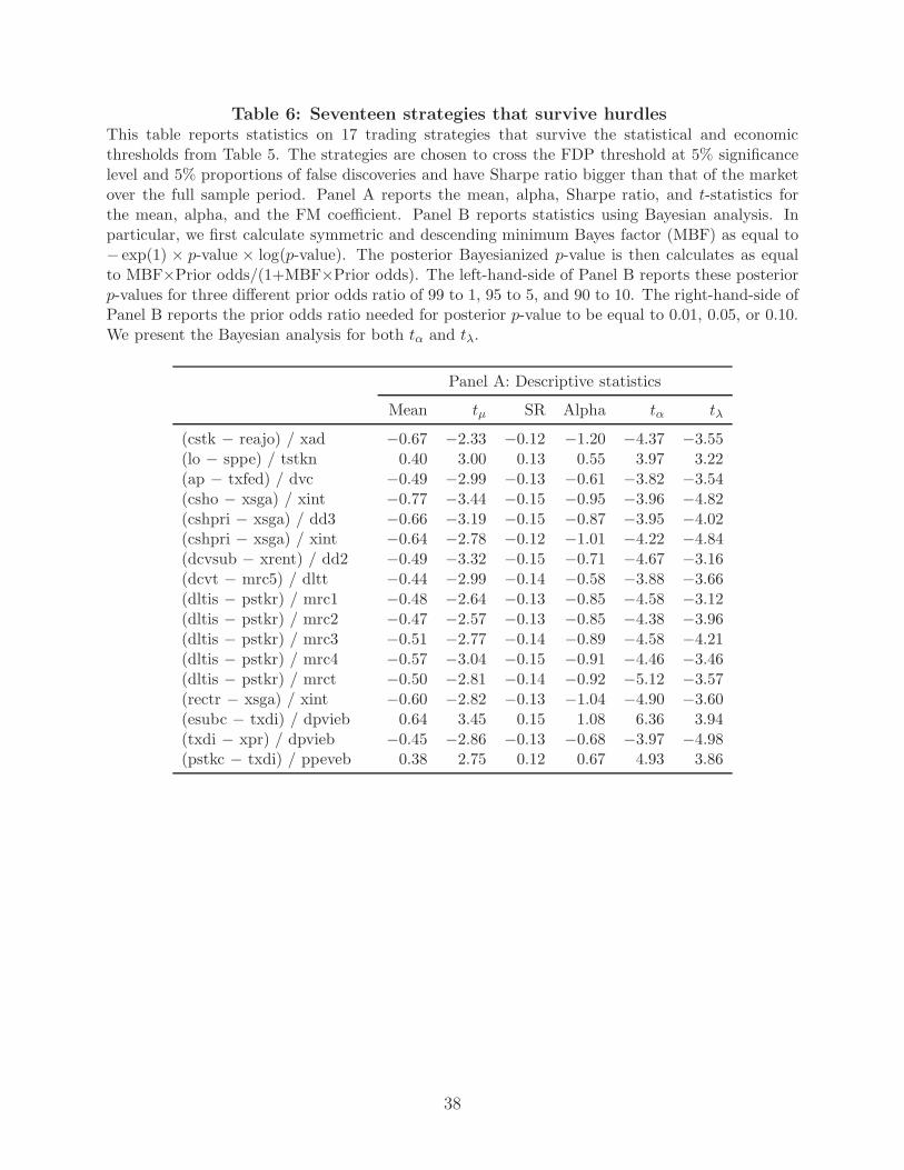
Table 6: Seventeen strategies that survive hurdlesThis table reports statistics on 17 trading strategies that survive the statistical and economicthresholds from Table 5. The strategies are chosen to cross the FDP threshold at 5% significancelevel and 5% proportions of false discoveries and have Sharpe ratio bigger than that of the marketover the full sample period. Panel A reports the mean, alpha, Sharpe ratio, and t-statistics forthe mean, alpha, and the FM coefficient. Panel B reports statistics using Bayesian analysis. Inparticular, we first calculate symmetric and descending minimum Bayes factor (MBF) as equal to− exp(1) × p-value × log(p-value). The posterior Bayesianized p-value is then calculates as equalto MBF×Prior odds/(1+MBF×Prior odds). The left-hand-side of Panel B reports these posteriorp-values for three different prior odds ratio of 99 to 1, 95 to 5, and 90 to 10. The right-hand-side ofPanel B reports the prior odds ratio needed for posterior p-value to be equal to 0.01, 0.05, or 0.10.We present the Bayesian analysis for both tα and tλ.

Panel A: Descriptive statistics

Mean tµ SR Alpha tα tλ

(cstk − reajo) / xad −0.67 −2.33 −0.12 −1.20 −4.37 −3.55(lo − sppe) / tstkn 0.40 3.00 0.13 0.55 3.97 3.22(ap − txfed) / dvc −0.49 −2.99 −0.13 −0.61 −3.82 −3.54(csho − xsga) / xint −0.77 −3.44 −0.15 −0.95 −3.96 −4.82(cshpri − xsga) / dd3 −0.66 −3.19 −0.15 −0.87 −3.95 −4.02(cshpri − xsga) / xint −0.64 −2.78 −0.12 −1.01 −4.22 −4.84(dcvsub − xrent) / dd2 −0.49 −3.32 −0.15 −0.71 −4.67 −3.16(dcvt − mrc5) / dltt −0.44 −2.99 −0.14 −0.58 −3.88 −3.66(dltis − pstkr) / mrc1 −0.48 −2.64 −0.13 −0.85 −4.58 −3.12(dltis − pstkr) / mrc2 −0.47 −2.57 −0.13 −0.85 −4.38 −3.96(dltis − pstkr) / mrc3 −0.51 −2.77 −0.14 −0.89 −4.58 −4.21(dltis − pstkr) / mrc4 −0.57 −3.04 −0.15 −0.91 −4.46 −3.46(dltis − pstkr) / mrct −0.50 −2.81 −0.14 −0.92 −5.12 −3.57(rectr − xsga) / xint −0.60 −2.82 −0.13 −1.04 −4.90 −3.60(esubc − txdi) / dpvieb 0.64 3.45 0.15 1.08 6.36 3.94(txdi − xpr) / dpvieb −0.45 −2.86 −0.13 −0.68 −3.97 −4.98(pstkc − txdi) / ppeveb 0.38 2.75 0.12 0.67 4.93 3.86

38

Panel B: Bayesian p-values

Posterior p-value Prior odds ratio

tα tλ tα tλ

Prior odds ratio Prior odds ratio Posterior p-value Posterior p-value99 to 1 95 to 5 90 to 10 99 to 1 95 to 5 90 to 10 0.01 0.05 0.10 0.01 0.05 0.10

(cstk − reajo) / xad 0.036 0.007 0.003 0.446 0.134 0.068 0.964 0.993 0.997 0.554 0.866 0.932(lo − sppe) / tstkn 0.156 0.034 0.017 0.700 0.309 0.175 0.844 0.966 0.983 0.300 0.691 0.825(ap − txfed) / dvc 0.241 0.058 0.028 0.458 0.139 0.071 0.759 0.942 0.972 0.542 0.861 0.929(csho − xsga) / xint 0.162 0.036 0.017 0.005 0.001 0.000 0.838 0.964 0.983 0.995 0.999 1.000(cshpri − xsga) / dd3 0.165 0.037 0.018 0.133 0.029 0.014 0.835 0.963 0.982 0.867 0.971 0.986(cshpri − xsga) / xint 0.064 0.013 0.006 0.005 0.001 0.000 0.936 0.987 0.994 0.995 0.999 1.000(dcvsub − xrent) / dd2 0.010 0.002 0.001 0.731 0.343 0.198 0.990 0.998 0.999 0.269 0.657 0.802(dcvt − mrc5) / dltt 0.202 0.046 0.023 0.360 0.097 0.049 0.798 0.954 0.977 0.640 0.903 0.951(dltis − pstkr) / mrc1 0.015 0.003 0.001 0.753 0.369 0.217 0.985 0.997 0.999 0.247 0.631 0.783(dltis − pstkr) / mrc2 0.035 0.007 0.003 0.162 0.036 0.017 0.965 0.993 0.997 0.838 0.964 0.983(dltis − pstkr) / mrc3 0.015 0.003 0.001 0.067 0.014 0.006 0.985 0.997 0.999 0.933 0.986 0.994(dltis − pstkr) / mrc4 0.025 0.005 0.002 0.521 0.173 0.090 0.975 0.995 0.998 0.479 0.827 0.910(dltis − pstkr) / mrct 0.001 0.000 0.000 0.436 0.129 0.066 0.999 1.000 1.000 0.564 0.871 0.934(rectr − xsga) / xint 0.004 0.001 0.000 0.408 0.117 0.059 0.996 0.999 1.000 0.592 0.883 0.941(esubc − txdi) / dpvieb 0.000 0.000 0.000 0.172 0.038 0.019 1.000 1.000 1.000 0.828 0.962 0.981(txdi − xpr) / dpvieb 0.157 0.034 0.017 0.002 0.000 0.000 0.843 0.966 0.983 0.998 1.000 1.000(pstkc − txdi) / ppeveb 0.003 0.001 0.000 0.216 0.050 0.024 0.997 0.999 1.000 0.784 0.950 0.976

39

Table 7: Robustness checks: Descriptive statisticsThis table reports cross-sectional mean, median, standard deviation, minimum, and maximum of alpha and Fama-MacBeth t-statisticfor (i) sample including all stocks) and (ii) alternative factor models. We use the three-factor model of Fama and French (1993) (FF),six-factor model of Barillas and Shanken (2015) (BS), and the four-factor model of Hou, Xue and Zhang (2015) augmented with themomentum factor (HXZ). We report alpha t-statistics in Panel A and Fama-MacBeth t-statistics in Panel B. We also report the numberand percentage of strategies that cross specific thresholds in each panel.

Panel A: Alpha t-statistic

N Mean Median Std Min Max |tα| > 1.96 |tα| > 2.57

# % # %

All stocks 2,090,365 −0.18 −0.18 1.63 −7.44 8.56 491,550 23.52 250,258 11.97FF3 2,090,365 −0.41 −0.44 1.47 −6.09 6.85 428,502 20.50 188,911 9.04BS 2,090,365 −0.09 −0.12 2.42 −7.94 7.73 958,043 45.83 673,077 32.20HXZ 2,090,365 −0.15 −0.14 1.73 −6.33 6.51 583,995 27.94 302,648 14.48

Panel B: Fama-MacBeth t-statistic

N Mean Median Std Min Max |tλ| > 1.96 |tλ| > 2.57

# % # %

All stocks 2,090,365 0.13 0.14 2.06 −12.91 12.49 684,108 32.73 424,315 20.30FF3 2,090,365 −0.03 −0.03 1.33 −7.17 7.30 280,523 13.42 122,560 5.86BS 2,090,365 0.11 0.11 1.99 −10.99 11.35 655,539 31.36 398,040 19.04HXZ 2,090,365 0.11 0.12 1.99 −11.30 11.14 662,381 31.69 404,239 19.34

40

Table 8: Robustness checks: Statistical and economic thresholdsThe table reports statistical thresholds for alpha and Fama-MacBeth t-statistics based on the FDP-StepM method (with significance equal to 5% and false discovery proportion of 5%) as well as thenumber of strategies that qualify based on economic hurdles based on the strategy Sharpe ratiosrelative to the market Sharpe ratio (in the same manner as in Table 5. Quantities are reportedfor the four robustness check cases presented in Table 7 (i.e., Fama and French (2015) five-factormodel together with the momentum factor for all stocks (All stocks), Fama and French (1993) threefactor model (FF3), Barillas and Shanken (2015) six-factor model (BS), and Hou, Xue and Zhang(2015) factor model together with the momentum factor (HXZ)).

0 to SRM/2 to SRM to More thantα tλ SRM/2 SRM 2×SRM 2×SRM

All stocks 3.98 3.04 Full sample 109 180 433 7Full sample and halves 50 47 80 0

FF3 4.28 3.95 Full sample 0 9 37 1Full sample and halves 0 4 13 0

BS 2.76 3.08 Full sample 3,955 917 80 0Full sample and halves 1,833 167 14 0

HXZ 3.85 3.08 Full sample 426 131 17 0Full sample and halves 209 25 1 0

41

Table A1: Basic variables used to construct trading strategies# Short Long # Short Long

1 aco Current Assets - Other - Total 61 idit Interest and Related Income - Total2 acox Current Assets - Other - Sundry 62 intan Intangible Assets - Total3 act Current Assets - Total 63 intc Interest Capitalized4 am Amortization of Intangibles 64 invfg Inventories - Finished Goods5 ao Assets - Other 65 invrm Inventories - Raw Materials6 aox Assets - Other - Sundry 66 invt Inventories - Total7 aqs Acquisitions - Sales Contribution 67 invwip Inventories - Work In Process8 at Assets - Total 68 itcb Investment Tax Credit (Balance Sheet)9 bkvlps Book Value Per Share 69 itci Investment Tax Credit (Income Account)10 caps Capital Surplus-Share Premium Reserve 70 ivaeq Investment and Advances - Equity11 capx Capital Expenditures 71 ivao Investment and Advances - Other12 capxv Capital Expend Property, Plant and Equipment Schd V 72 ivst Short-Term Investments - Total13 ceq Common-Ordinary Equity - Total 73 lco Current Liabilities - Other - Total14 ceql Common Equity - Liquidation Value 74 lcox Current Liabilities - Other - Sundry15 ceqt Common Equity - Tangible 75 lct Current Liabilities - Total16 ch Cash 76 lifr LIFO Reserve17 che Cash and Short-Term Investments 77 lifrp LIFO Reserve - Prior18 chech Cash and Cash Equivalents - Increase-(Decrease) 78 lse Liabilities and Stockholders Equity - Total19 cogs Cost of Goods Sold 79 lt Liabilities - Total20 cshfd Common Shares Used to Calc Earnings Per Share - Fully Diluted 80 mib Noncontrolling Interest (Balance Sheet)21 csho Common Shares Outstanding 81 mibt Noncontrolling Interests - Total - Balance Sheet22 cshpri Common Shares Used to Calculate Earnings Per Share - Basic 82 mii Noncontrolling Interest (Income Account)23 cshr Common-Ordinary Shareholders 83 mrc1 Rental Commitments - Minimum - 1st Year24 cstk Common-Ordinary Stock (Capital) 84 mrc2 Rental Commitments - Minimum - 2nd Year25 cstkcv Common Stock-Carrying Value 85 mrc3 Rental Commitments - Minimum - 3rd Year26 cstke Common Stock Equivalents - Dollar Savings 86 mrc4 Rental Commitments - Minimum - 4th Year27 dc Deferred Charges 87 mrc5 Rental Commitments - Minimum - 5th Year28 dcpstk Convertible Debt and Preferred Stock 88 mrct Rental Commitments - Minimum - 5 Year Total29 dcvsr Debt - Senior Convertible 89 msa Marketable Securities Adjustment30 dcvsub Debt - Subordinated Convertible 90 ni Net Income (Loss)31 dcvt Debt - Convertible 91 niadj Net Income Adjusted for Common-Ordinary Stock (Capital) Equivalents32 dd5 Debt - Due in 5th Year 92 nopi Nonoperating Income (Expense)33 dlto Other Long-term Debt 93 nopio Nonoperating Income (Expense) - Other34 dltp Long-Term Debt - Tied to Prime 94 np Notes Payable - Short-Term Borrowings35 dltt Long-Term Debt - Total 95 ob Order Backlog36 dm Debt - Mortgages Other Secured 96 oiadp Operating Income After Depreciation37 dn Debt - Notes 97 oibdp Operating Income Before Depreciation38 dp Depreciation and Amortization 98 pi Pretax Income39 dpact Depreciation, Depletion and Amortization (Accumulated) 99 ppegt Property, Plant and Equipment - Total (Gross)40 dpc Depreciation and Amortization (Cash Flow) 100 ppent Property, Plant and Equipment - Total (Net)41 dpvieb Depreciation (Accumulated) - Ending Balance (Schedule VI) 101 ppeveb Property, Plant, and Equipment - Ending Balance (Schedule V)42 ds Debt-Subordinated 102 prstkc Purchase of Common and Preferred Stock43 dv Cash Dividends (Cash Flow) 103 pstk Preferred-Preference Stock (Capital) - Total44 dvc Dividends Common-Ordinary 104 pstkc Preferred Stock - Convertible45 dvp Dividends - Preferred-Preference 105 pstkl Preferred Stock - Liquidating Value46 dvpa Preferred Dividends in Arrears 106 pstkn Preferred-Preference Stock - Nonredeemable47 dvt Dividends - Total 107 pstkr Preferred-Preference Stock - Redeemable48 ebit Earnings Before Interest and Taxes 108 pstkrv Preferred Stock - Redemption Value49 ebitda Earnings Before Interest 109 re Retained Earnings50 emp Employees 110 rea Retained Earnings - Restatement51 esub Equity in Earnings - Unconsolidated Subsidiaries 111 reajo Retained Earnings - Other Adjustments52 esubc Equity in Net Loss - Earnings 112 recco Receivables - Current - Other53 fca Foreign Exchange Income (Loss) 113 recd Receivables - Estimated Doubtful54 fopo Funds from Operations - Other 114 recta Retained Earnings - Cumulative Translation Adjustment55 gp Gross Profit (Loss) 115 rectr Receivables - Trade56 ib Income Before Extraordinary Items 116 reuna Retained Earnings - Unadjusted57 ibadj Income Before Extraordinary Items - Adjusted for Common Stock Equivalents 117 revt Revenue - Total58 ibc Income Before Extraordinary Items (Cash Flow) 118 sale Sales-Turnover (Net)59 ibcom Income Before Extraordinary Items - Available for Common 119 seq Stockholders Equity - Parent60 icapt Invested Capital - Total 120 spi Special Items

42

# Short Long # Short Long

121 sppe Sale of Property 139 xad Advertising Expense122 sstk Sale of Common and Preferred Stock 140 xido Extraordinary Items and Discontinued Operations123 tstkc Treasury Stock - Common 141 xidoc Extraordinary Items and Discontinued Operations (Cash Flow)124 tstkn Treasury Stock - Number of Common Shares 142 xint Interest and Related Expense - Total125 tstkp Treasury Stock - Preferrred 143 xlr Staff Expense - Total126 txc Income Taxes - Current 144 xopr Operating Expenses - Total127 txdb Deferred Taxes (Balance Sheet) 145 xpp Prepaid Expenses128 txdc Deferred Taxes (Cash Flow) 146 xpr Pension and Retirement Expense129 txdi Income Taxes - Deferred 147 xrd Research and Development Expense130 txditc Deferred Taxes and Investment Tax Credit 148 xrdp Research Development - Prior131 txfed Income Taxes - Federal 149 xrent Rental Expense132 txfo Income Taxes - Foreign 150 xsga Selling, General and Administrative Expense133 txp Income Taxes Payable 151 ret1 1m Past Return134 txs Income Taxes - State 152 ret3 3m Past Return135 txt Income Taxes - Total 153 ret6 6m Past Return136 txw Excise Taxes 154 ret9 9m Past Return137 wcap Working Capital (Balance Sheet) 155 ret12 1y Past Return138 xacc Accrued Expenses 156 vol 1y Return Volatility

43

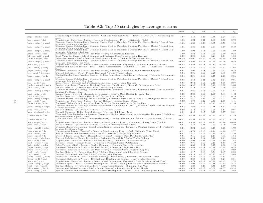
Table A2: Top 50 strategies by average returnsMean tµ SR α tα tλ

(caps - chech) / xad(Capital Surplus-Share Premium Reserve - Cash and Cash Equivalents - Increase-(Decrease)) / Advertising Ex-pense

−1.07 −4.40 −0.23 −0.55 −2.27 −1.21

(aqs - xrdp) / dvt (Acquisitions - Sales Contribution - Research Development - Prior) / Dividends - Total −1.06 −4.04 −0.21 −1.03 −3.72 3.70

(csho - cshpri) / mrc1 (Common Shares Outstanding - Common Shares Used to Calculate Earnings Per Share - Basic) / Rental Com-mitments - Minimum - 1st Year

−1.05 −4.38 −0.20 −0.37 −1.79 1.18

(csho - cshpri) / mrc4 (Common Shares Outstanding - Common Shares Used to Calculate Earnings Per Share - Basic) / Rental Com-mitments - Minimum - 4th Year

−1.05 −4.36 −0.20 −0.34 −1.57 0.49

(csho - cshpri) / mrc2 (Common Shares Outstanding - Common Shares Used to Calculate Earnings Per Share - Basic) / Rental Com-mitments - Minimum - 2nd Year

−1.00 −4.04 −0.18 −0.29 −1.39 1.89

(dvpa - ret6) / xad (Preferred Dividends in Arrears - 6m Past Return) / Advertising Expense −1.00 −3.82 −0.18 −0.60 −2.00 −0.23(bkvlps - sstk) / xad (Book Value Per Share - Sale of Common and Preferred Stock) / Advertising Expense 0.99 3.98 0.18 0.24 0.91 1.98(intan - xrdp) / dvc (Intangible Assets - Total - Research Development - Prior) / Dividends Common-Ordinary −0.99 −4.07 −0.20 −0.96 −3.84 −1.69

(csho - cshpri) / mrc3 (Common Shares Outstanding - Common Shares Used to Calculate Earnings Per Share - Basic) / Rental Com-mitments - Minimum - 3rd Year

−0.98 −3.92 −0.18 −0.26 −1.26 0.48

(aqs - xrd) / dvc (Acquisitions - Sales Contribution - Research and Development Expense) / Dividends Common-Ordinary −0.95 −3.84 −0.18 −0.82 −3.09 1.52

(idit - mrc1) / invfg (Interest and Related Income - Total - Rental Commitments - Minimum - 1st Year) / Inventories - FinishedGoods

−0.95 −3.16 −0.16 −0.29 −1.07 −1.03

(dvpa - ret6) / xsga (Preferred Dividends in Arrears - 6m Past Return) / Selling, General and Administrative Expense −0.94 −3.90 −0.18 −0.55 −2.41 0.22(lct - xpp) / dvolume (Current Liabilities - Total - Prepaid Expenses) / Dollar Traded Volume 0.94 3.65 0.16 0.25 1.40 1.99

(caps - xsga) / xrdp (Capital Surplus-Share Premium Reserve - Selling, General and Administrative Expense) / Research Development- Prior

−0.94 −3.91 −0.19 −0.75 −2.95 −0.35

(csho - cshpri) / mrct (Common Shares Outstanding - Common Shares Used to Calculate Earnings Per Share - Basic) / Rental Com-mitments - Minimum - 5 Year Total

−0.93 −4.52 −0.21 −0.42 −2.14 0.91

(txw - xrd) / xad (Excise Taxes - Research and Development Expense) / Advertising Expense 0.93 2.52 0.13 −0.18 −0.56 −2.07(esubc - reuna) / xrdp (Equity in Net Loss - Earnings - Retained Earnings - Unadjusted) / Research Development - Prior −0.93 −3.28 −0.17 −0.43 −1.95 −2.35(ret6 - vol) / xad (6m Past Return - 1y Return Volatility) / Advertising Expense 0.93 4.18 0.19 0.78 3.36 2.84

(csho - mrc2) / cshpri(Common Shares Outstanding - Rental Commitments - Minimum - 2nd Year) / Common Shares Used to CalculateEarnings Per Share - Basic

−0.93 −3.86 −0.18 −0.21 −1.17 −1.67

(txdi - xrdp) / dv (Income Taxes - Deferred - Research Development - Prior) / Cash Dividends (Cash Flow) −0.93 −3.30 −0.16 −1.33 −5.41 1.42(ret6 - vol) / act (6m Past Return - 1y Return Volatility) / Current Assets - Total 0.93 4.15 0.18 0.55 2.32 0.13(csho - ret6) / cshpri (Common Shares Outstanding - 6m Past Return) / Common Shares Used to Calculate Earnings Per Share - Basic −0.92 −5.41 −0.24 −0.30 −1.73 1.96(aqs - ret6) / txs (Acquisitions - Sales Contribution - 6m Past Return) / Income Taxes - State −0.92 −4.69 −0.22 −0.40 −2.03 1.45(dvpa - ret6) / cshr (Preferred Dividends in Arrears - 6m Past Return) / Common-Ordinary Shareholders −0.92 −4.07 −0.19 −0.45 −2.12 −1.16

(csho - mrc3) / cshpri(Common Shares Outstanding - Rental Commitments - Minimum - 3rd Year) / Common Shares Used to CalculateEarnings Per Share - Basic

−0.92 −3.63 −0.17 −0.18 −0.97 −1.38

(ret6 - vol) / rectr (6m Past Return - 1y Return Volatility) / Receivables - Trade 0.92 4.12 0.19 0.65 2.84 2.05(xpp - dvolume) / lct (Prepaid Expenses - Dollar Traded Volume) / Current Liabilities - Total 0.91 3.48 0.15 0.21 1.17 2.61

(chech - xsga) / lse(Cash and Cash Equivalents - Increase-(Decrease) - Selling, General and Administrative Expense) / Liabilitiesand Stockholders Equity - Total

−0.91 −4.34 −0.22 −0.42 −2.17 −1.35

(chech - xsga) / at (Cash and Cash Equivalents - Increase-(Decrease) - Selling, General and Administrative Expense) / Assets -Total

−0.91 −4.34 −0.22 −0.42 −2.17 −1.35

(aqs - xrdp) / cstk (Acquisitions - Sales Contribution - Research Development - Prior) / Common-Ordinary Stock (Capital) −0.91 −3.33 −0.17 −1.13 −3.86 −0.86(ret6 - vol) / cshr (6m Past Return - 1y Return Volatility) / Common-Ordinary Shareholders 0.91 4.49 0.21 0.52 2.79 1.59

(csho - mrc1) / cshpri(Common Shares Outstanding - Rental Commitments - Minimum - 1st Year) / Common Shares Used to CalculateEarnings Per Share - Basic

−0.91 −3.94 −0.18 −0.18 −1.03 −1.79

(nopi - xrdp) / dv (Nonoperating Income (Expense) - Research Development - Prior) / Cash Dividends (Cash Flow) −0.91 −3.73 −0.18 −1.14 −4.68 2.77(sstk - ret9) / xad (Sale of Common and Preferred Stock - 9m Past Return) / Advertising Expense −0.91 −3.77 −0.17 −0.19 −0.77 −2.10(txdc - xrdp) / dv (Deferred Taxes (Cash Flow) - Research Development - Prior) / Cash Dividends (Cash Flow) −0.91 −3.11 −0.15 −1.17 −4.43 1.84(lct - recd) / dvolume (Current Liabilities - Total - Receivables - Estimated Doubtful) / Dollar Traded Volume 0.90 3.14 0.14 0.13 0.61 2.05(aqs - ret3) / dvc (Acquisitions - Sales Contribution - 3m Past Return) / Dividends Common-Ordinary −0.90 −4.99 −0.23 −0.46 −2.69 1.83(revt - tstkc) / csho (Revenue - Total - Treasury Stock - Common) / Common Shares Outstanding 0.90 3.35 0.17 0.15 0.85 −1.19(sale - tstkc) / csho (Sales-Turnover (Net) - Treasury Stock - Common) / Common Shares Outstanding 0.90 3.35 0.17 0.15 0.85 −1.19(dvpa - ret6) / xopr (Preferred Dividends in Arrears - 6m Past Return) / Operating Expenses - Total −0.90 −3.84 −0.18 −0.48 −2.08 0.33(dvpa - ret3) / cstk (Preferred Dividends in Arrears - 3m Past Return) / Common-Ordinary Stock (Capital) −0.90 −4.17 −0.19 −0.79 −3.51 2.92(ret6 - vol) / xsga (6m Past Return - 1y Return Volatility) / Selling, General and Administrative Expense 0.90 4.17 0.18 0.54 2.47 −0.29(intc - ret6) / xad (Interest Capitalized - 6m Past Return) / Advertising Expense −0.90 −3.19 −0.15 −0.83 −3.17 3.03(invfg - reuna) / xrdp (Inventories - Finished Goods - Retained Earnings - Unadjusted) / Research Development - Prior −0.90 −3.19 −0.16 −0.35 −1.64 −1.77(dvpa - xrd) / xad (Preferred Dividends in Arrears - Research and Development Expense) / Advertising Expense 0.90 2.88 0.14 −0.06 −0.21 0.61(aqs - xrd) / dv (Acquisitions - Sales Contribution - Research and Development Expense) / Cash Dividends (Cash Flow) −0.90 −3.74 −0.18 −0.86 −3.42 2.74(icapt - xrdp) / xsga (Invested Capital - Total - Research Development - Prior) / Selling, General and Administrative Expense −0.90 −3.94 −0.19 −0.88 −3.92 2.34(ret6 - vol) / mrc2 (6m Past Return - 1y Return Volatility) / Rental Commitments - Minimum - 2nd Year 0.89 4.28 0.20 0.59 2.87 0.76(idit - xrent) / invfg (Interest and Related Income - Total - Rental Expense) / Inventories - Finished Goods −0.89 −3.29 −0.15 −0.09 −0.37 −3.14(sstk - xrdp) / dv (Sale of Common and Preferred Stock - Research Development - Prior) / Cash Dividends (Cash Flow) −0.89 −3.77 −0.18 −0.71 −2.99 2.92

44

Table A3: Top 50 strategies by average returns t-statisticMean tµ SR α tα tλ

(csho - ret6) / cshpri (Common Shares Outstanding - 6m Past Return) / Common Shares Used to Calculate Earnings Per Share - Basic −0.92 −5.41 −0.24 −0.30 −1.73 1.96(csho - ret3) / cshpri (Common Shares Outstanding - 3m Past Return) / Common Shares Used to Calculate Earnings Per Share - Basic −0.89 −5.03 −0.22 −0.23 −1.38 3.07(dd4 - dltis) / ppegt (Debt - Due in 4th Year - Long-Term Debt - Issuance) / Property, Plant and Equipment - Total (Gross) 0.59 5.01 0.23 0.52 4.73 1.45(aqs - ret3) / dvc (Acquisitions - Sales Contribution - 3m Past Return) / Dividends Common-Ordinary −0.90 −4.99 −0.23 −0.46 −2.69 1.83(csho - ret9) / cshpri (Common Shares Outstanding - 9m Past Return) / Common Shares Used to Calculate Earnings Per Share - Basic −0.83 −4.97 −0.22 −0.37 −2.21 1.90(aqs - ret3) / dv (Acquisitions - Sales Contribution - 3m Past Return) / Cash Dividends (Cash Flow) −0.83 −4.82 −0.22 −0.40 −2.54 1.55(aqs - lct) / size (Acquisitions - Sales Contribution - Current Liabilities - Total) / Market Capitalization −0.84 −4.75 −0.22 −0.46 −2.89 −2.24(aqs - ret6) / txs (Acquisitions - Sales Contribution - 6m Past Return) / Income Taxes - State −0.92 −4.69 −0.22 −0.40 −2.03 1.45(recco - ret6) / dv (Receivables - Current - Other - 6m Past Return) / Cash Dividends (Cash Flow) −0.81 −4.68 −0.21 −0.56 −3.33 −1.56(msa - ret3) / dv (Marketable Securities Adjustment - 3m Past Return) / Cash Dividends (Cash Flow) −0.79 −4.68 −0.22 −0.37 −2.12 −1.43(ch - sstk) / txt (Cash - Sale of Common and Preferred Stock) / Income Taxes - Total 0.65 4.67 0.21 0.32 2.05 −0.49

(cshpri - do) / csho(Common Shares Used to Calculate Earnings Per Share - Basic - Discontinued Operations) / Common SharesOutstanding

0.57 4.66 0.21 0.21 1.76 2.82

(np - ret3) / dv (Notes Payable - Short-Term Borrowings - 3m Past Return) / Cash Dividends (Cash Flow) −0.73 −4.65 −0.20 −0.46 −3.03 −2.01(dd4 - dltis) / ch (Debt - Due in 4th Year - Long-Term Debt - Issuance) / Cash 0.51 4.64 0.21 0.38 3.29 −1.71(np - ret3) / dvt (Notes Payable - Short-Term Borrowings - 3m Past Return) / Dividends - Total −0.72 −4.64 −0.20 −0.42 −2.85 −0.34(rea - ret3) / dv (Retained Earnings - Restatement - 3m Past Return) / Cash Dividends (Cash Flow) −0.76 −4.62 −0.20 −0.37 −2.35 0.45

(ap - cshpri) / xrd(Accounts Payable - Trade - Common Shares Used to Calculate Earnings Per Share - Basic) / Research andDevelopment Expense

0.73 4.57 0.20 0.60 3.72 2.73

(aqc - ret3) / dvt (Acquisitions - 3m Past Return) / Dividends - Total −0.72 −4.57 −0.20 −0.53 −3.21 0.78(dvc - ret3) / dv (Dividends Common-Ordinary - 3m Past Return) / Cash Dividends (Cash Flow) −0.76 −4.57 −0.20 −0.35 −2.15 −2.01(ap - csho) / xrd (Accounts Payable - Trade - Common Shares Outstanding) / Research and Development Expense 0.75 4.56 0.20 0.60 3.61 2.47(dvc - ret3) / dvt (Dividends Common-Ordinary - 3m Past Return) / Dividends - Total −0.75 −4.56 −0.20 −0.39 −2.44 0.31(intc - ret3) / dvt (Interest Capitalized - 3m Past Return) / Dividends - Total −0.79 −4.55 −0.21 −0.48 −2.78 −1.68(recco - ret3) / dv (Receivables - Current - Other - 3m Past Return) / Cash Dividends (Cash Flow) −0.76 −4.55 −0.20 −0.63 −3.75 −1.22(msa - ret3) / dvc (Marketable Securities Adjustment - 3m Past Return) / Dividends Common-Ordinary −0.76 −4.55 −0.21 −0.24 −1.43 0.34(dc - ret3) / dv (Deferred Charges - 3m Past Return) / Cash Dividends (Cash Flow) −0.81 −4.54 −0.21 −0.55 −3.06 −2.09(dvpa - ret3) / dvt (Preferred Dividends in Arrears - 3m Past Return) / Dividends - Total −0.78 −4.53 −0.21 −0.44 −2.65 −1.92(aqs - ret3) / dvt (Acquisitions - Sales Contribution - 3m Past Return) / Dividends - Total −0.77 −4.52 −0.21 −0.37 −2.32 0.76

(csho - cshpri) / mrct (Common Shares Outstanding - Common Shares Used to Calculate Earnings Per Share - Basic) / Rental Com-mitments - Minimum - 5 Year Total

−0.93 −4.52 −0.21 −0.42 −2.14 0.91

(aqs - ret3) / txs (Acquisitions - Sales Contribution - 3m Past Return) / Income Taxes - State −0.87 −4.51 −0.21 −0.49 −2.44 1.56(dd4 - dltis) / ap (Debt - Due in 4th Year - Long-Term Debt - Issuance) / Accounts Payable - Trade 0.49 4.51 0.21 0.35 3.36 0.66

(csho - txr) / cshpri (Common Shares Outstanding - Income Tax Refund) / Common Shares Used to Calculate Earnings Per Share -Basic

−0.73 −4.51 −0.20 −0.21 −1.36 0.19

(dd3 - dltis) / ppegt (Debt - Due in 3rd Year - Long-Term Debt - Issuance) / Property, Plant and Equipment - Total (Gross) 0.52 4.50 0.21 0.45 3.85 2.07(ret6 - vol) / cshr (6m Past Return - 1y Return Volatility) / Common-Ordinary Shareholders 0.91 4.49 0.21 0.52 2.79 1.59

(dd4 - dltis) / ppeveb(Debt - Due in 4th Year - Long-Term Debt - Issuance) / Property, Plant, and Equipment - Ending Balance(Schedule V)

0.54 4.49 0.21 0.48 4.14 0.35

(csho - ret1) / cshpri (Common Shares Outstanding - 1m Past Return) / Common Shares Used to Calculate Earnings Per Share - Basic −0.76 −4.49 −0.20 −0.16 −1.07 3.86(dd4 - dltis) / gp (Debt - Due in 4th Year - Long-Term Debt - Issuance) / Gross Profit (Loss) 0.54 4.48 0.20 0.48 3.96 −3.63(lco - sstk) / cshr (Current Liabilities - Other - Total - Sale of Common and Preferred Stock) / Common-Ordinary Shareholders 0.63 4.48 0.21 0.41 3.00 −2.72

(csho - cstke) / cshpri(Common Shares Outstanding - Common Stock Equivalents - Dollar Savings) / Common Shares Used to CalculateEarnings Per Share - Basic

−0.77 −4.47 −0.20 −0.20 −1.31 2.93

(ret6 - vol) / revt (6m Past Return - 1y Return Volatility) / Revenue - Total 0.89 4.45 0.20 0.41 2.03 0.58(ret6 - vol) / sale (6m Past Return - 1y Return Volatility) / Sales-Turnover (Net) 0.89 4.45 0.20 0.41 2.03 0.58(dd5 - dltis) / ch (Debt - Due in 5th Year - Long-Term Debt - Issuance) / Cash 0.46 4.44 0.20 0.40 3.60 −1.14

(csho - idit) / cshpri(Common Shares Outstanding - Interest and Related Income - Total) / Common Shares Used to CalculateEarnings Per Share - Basic

−0.83 −4.44 −0.20 −0.67 −3.63 1.55

(ret6 - vol) / dp (6m Past Return - 1y Return Volatility) / Depreciation and Amortization 0.85 4.43 0.20 0.82 4.31 2.46(ch - ds) / dvolume (Cash - Debt-Subordinated) / Dollar Traded Volume 0.55 4.42 0.19 0.50 4.01 −0.15

(cstk - epsfx) / dvt (Common-Ordinary Stock (Capital) - Earnings Per Share (Diluted) - Excluding Extraordinary Items) / Dividends- Total

−0.61 −4.41 −0.19 −0.31 −2.35 2.00

(caps - chech) / xad(Capital Surplus-Share Premium Reserve - Cash and Cash Equivalents - Increase-(Decrease)) / Advertising Ex-pense

−1.07 −4.40 −0.23 −0.55 −2.27 −1.21

(epsfx - sstk) / txp(Earnings Per Share (Diluted) - Excluding Extraordinary Items - Sale of Common and Preferred Stock) / IncomeTaxes Payable

0.50 4.39 0.19 0.26 2.11 −2.15

(aqc - ret6) / dv (Acquisitions - 6m Past Return) / Cash Dividends (Cash Flow) −0.70 −4.39 −0.19 −0.39 −2.36 −0.35(tstk - ret3) / dv (Treasury Stock - Total (All Capital) - 3m Past Return) / Cash Dividends (Cash Flow) −0.77 −4.39 −0.19 −0.62 −3.83 1.05

(csho - cshpri) / mrc1 (Common Shares Outstanding - Common Shares Used to Calculate Earnings Per Share - Basic) / Rental Com-mitments - Minimum - 1st Year

−1.05 −4.38 −0.20 −0.37 −1.79 1.18

45

Table A4: Top 50 strategies by Sharpe ratioMean tµ SR α tα tλ

(csho - ret6) / cshpri (Common Shares Outstanding - 6m Past Return) / Common Shares Used to Calculate Earnings Per Share - Basic −0.92 −5.41 −0.24 −0.30 −1.73 1.96(dd4 - dltis) / ppegt (Debt - Due in 4th Year - Long-Term Debt - Issuance) / Property, Plant and Equipment - Total (Gross) 0.59 5.01 0.23 0.52 4.73 1.45

(caps - chech) / xad(Capital Surplus-Share Premium Reserve - Cash and Cash Equivalents - Increase-(Decrease)) / Advertising Ex-pense

−1.07 −4.40 −0.23 −0.55 −2.27 −1.21

(aqs - ret3) / dvc (Acquisitions - Sales Contribution - 3m Past Return) / Dividends Common-Ordinary −0.90 −4.99 −0.23 −0.46 −2.69 1.83

(chech - xsga) / lse(Cash and Cash Equivalents - Increase-(Decrease) - Selling, General and Administrative Expense) / Liabilitiesand Stockholders Equity - Total

−0.91 −4.34 −0.22 −0.42 −2.17 −1.35

(chech - xsga) / at (Cash and Cash Equivalents - Increase-(Decrease) - Selling, General and Administrative Expense) / Assets -Total

−0.91 −4.34 −0.22 −0.42 −2.17 −1.35

(csho - ret3) / cshpri (Common Shares Outstanding - 3m Past Return) / Common Shares Used to Calculate Earnings Per Share - Basic −0.89 −5.03 −0.22 −0.23 −1.38 3.07(aqs - ret3) / dv (Acquisitions - Sales Contribution - 3m Past Return) / Cash Dividends (Cash Flow) −0.83 −4.82 −0.22 −0.40 −2.54 1.55(aqs - lct) / size (Acquisitions - Sales Contribution - Current Liabilities - Total) / Market Capitalization −0.84 −4.75 −0.22 −0.46 −2.89 −2.24

(dvpa - recta) / ivao (Preferred Dividends in Arrears - Retained Earnings - Cumulative Translation Adjustment) / Investment andAdvances - Other

−0.69 −4.30 −0.22 −0.51 −3.10 1.31

(csho - ret9) / cshpri (Common Shares Outstanding - 9m Past Return) / Common Shares Used to Calculate Earnings Per Share - Basic −0.83 −4.97 −0.22 −0.37 −2.21 1.90(aqs - ret6) / txs (Acquisitions - Sales Contribution - 6m Past Return) / Income Taxes - State −0.92 −4.69 −0.22 −0.40 −2.03 1.45(msa - ret3) / dv (Marketable Securities Adjustment - 3m Past Return) / Cash Dividends (Cash Flow) −0.79 −4.68 −0.22 −0.37 −2.12 −1.43(dcvsr - recta) / ivch (Debt - Senior Convertible - Retained Earnings - Cumulative Translation Adjustment) / Increase in Investments −0.71 −4.16 −0.21 −0.33 −1.99 −0.07(dd4 - dltis) / ch (Debt - Due in 4th Year - Long-Term Debt - Issuance) / Cash 0.51 4.64 0.21 0.38 3.29 −1.71(intc - ret3) / dvt (Interest Capitalized - 3m Past Return) / Dividends - Total −0.79 −4.55 −0.21 −0.48 −2.78 −1.68(msa - ret3) / dvc (Marketable Securities Adjustment - 3m Past Return) / Dividends Common-Ordinary −0.76 −4.55 −0.21 −0.24 −1.43 0.34(dc - ret3) / dv (Deferred Charges - 3m Past Return) / Cash Dividends (Cash Flow) −0.81 −4.54 −0.21 −0.55 −3.06 −2.09(dvpa - ret3) / dvt (Preferred Dividends in Arrears - 3m Past Return) / Dividends - Total −0.78 −4.53 −0.21 −0.44 −2.65 −1.92

(dcvsr - recta) / ivao (Debt - Senior Convertible - Retained Earnings - Cumulative Translation Adjustment) / Investment and Advances- Other

−0.67 −4.10 −0.21 −0.45 −2.71 1.57

(aqs - ret3) / txs (Acquisitions - Sales Contribution - 3m Past Return) / Income Taxes - State −0.87 −4.51 −0.21 −0.49 −2.44 1.56(ret6 - vol) / cshr (6m Past Return - 1y Return Volatility) / Common-Ordinary Shareholders 0.91 4.49 0.21 0.52 2.79 1.59(lco - sstk) / cshr (Current Liabilities - Other - Total - Sale of Common and Preferred Stock) / Common-Ordinary Shareholders 0.63 4.48 0.21 0.41 3.00 −2.72(aqs - ret3) / dvt (Acquisitions - Sales Contribution - 3m Past Return) / Dividends - Total −0.77 −4.52 −0.21 −0.37 −2.32 0.76

(chech - mrc2) / txfed (Cash and Cash Equivalents - Increase-(Decrease) - Rental Commitments - Minimum - 2nd Year) / Income Taxes- Federal

−0.78 −3.98 −0.21 −0.50 −2.51 −3.28

(csho - cshpri) / mrct (Common Shares Outstanding - Common Shares Used to Calculate Earnings Per Share - Basic) / Rental Com-mitments - Minimum - 5 Year Total

−0.93 −4.52 −0.21 −0.42 −2.14 0.91

(recco - ret6) / dv (Receivables - Current - Other - 6m Past Return) / Cash Dividends (Cash Flow) −0.81 −4.68 −0.21 −0.56 −3.33 −1.56(aqs - xrdp) / dvt (Acquisitions - Sales Contribution - Research Development - Prior) / Dividends - Total −1.06 −4.04 −0.21 −1.03 −3.72 3.70(dd4 - dltis) / ap (Debt - Due in 4th Year - Long-Term Debt - Issuance) / Accounts Payable - Trade 0.49 4.51 0.21 0.35 3.36 0.66(ch - sstk) / txt (Cash - Sale of Common and Preferred Stock) / Income Taxes - Total 0.65 4.67 0.21 0.32 2.05 −0.49(dd3 - dltis) / ppegt (Debt - Due in 3rd Year - Long-Term Debt - Issuance) / Property, Plant and Equipment - Total (Gross) 0.52 4.50 0.21 0.45 3.85 2.07

(chech - mrct) / txfed (Cash and Cash Equivalents - Increase-(Decrease) - Rental Commitments - Minimum - 5 Year Total) / IncomeTaxes - Federal

−0.71 −3.96 −0.21 −0.47 −2.48 −2.29

(cshpri - do) / csho(Common Shares Used to Calculate Earnings Per Share - Basic - Discontinued Operations) / Common SharesOutstanding

0.57 4.66 0.21 0.21 1.76 2.82

(dd4 - dltis) / ppeveb(Debt - Due in 4th Year - Long-Term Debt - Issuance) / Property, Plant, and Equipment - Ending Balance(Schedule V)

0.54 4.49 0.21 0.48 4.14 0.35

(dm - xsga) / ebitda (Debt - Mortgages Other Secured - Selling, General and Administrative Expense) / Earnings Before Interest −0.67 −4.08 −0.20 −0.61 −3.01 3.14

(dm - xsga) / oibdp(Debt - Mortgages Other Secured - Selling, General and Administrative Expense) / Operating Income BeforeDepreciation

−0.67 −4.08 −0.20 −0.61 −3.01 3.14

(ivch - recta) / txfed (Increase in Investments - Retained Earnings - Cumulative Translation Adjustment) / Income Taxes - Federal −0.68 −4.01 −0.20 −0.31 −2.11 1.13(np - ret3) / dv (Notes Payable - Short-Term Borrowings - 3m Past Return) / Cash Dividends (Cash Flow) −0.73 −4.65 −0.20 −0.46 −3.03 −2.01(dd4 - dltis) / gp (Debt - Due in 4th Year - Long-Term Debt - Issuance) / Gross Profit (Loss) 0.54 4.48 0.20 0.48 3.96 −3.63(np - ret3) / dvt (Notes Payable - Short-Term Borrowings - 3m Past Return) / Dividends - Total −0.72 −4.64 −0.20 −0.42 −2.85 −0.34

(chech - xsga) / ebitda (Cash and Cash Equivalents - Increase-(Decrease) - Selling, General and Administrative Expense) / EarningsBefore Interest

−0.71 −4.00 −0.20 −0.26 −1.45 1.36

(chech - xsga) / oibdp(Cash and Cash Equivalents - Increase-(Decrease) - Selling, General and Administrative Expense) / OperatingIncome Before Depreciation

−0.71 −4.00 −0.20 −0.26 −1.45 1.36

(dcvt - recta) / ivch (Debt - Convertible - Retained Earnings - Cumulative Translation Adjustment) / Increase in Investments −0.69 −4.00 −0.20 −0.41 −2.61 0.09(chech - xrent) / txfed (Cash and Cash Equivalents - Increase-(Decrease) - Rental Expense) / Income Taxes - Federal −0.74 −3.99 −0.20 −0.39 −1.99 −2.25(rea - ret3) / dv (Retained Earnings - Restatement - 3m Past Return) / Cash Dividends (Cash Flow) −0.76 −4.62 −0.20 −0.37 −2.35 0.45(dd5 - dltis) / ch (Debt - Due in 5th Year - Long-Term Debt - Issuance) / Cash 0.46 4.44 0.20 0.40 3.60 −1.14(dvpa - ret3) / dvc (Preferred Dividends in Arrears - 3m Past Return) / Dividends Common-Ordinary −0.76 −4.38 −0.20 −0.42 −2.51 1.11(ret6 - vol) / xrdp (6m Past Return - 1y Return Volatility) / Research Development - Prior 0.85 4.14 0.20 0.96 4.81 0.64

(chech - sstk) / dpvieb(Cash and Cash Equivalents - Increase-(Decrease) - Sale of Common and Preferred Stock) / Depreciation (Accu-mulated) - Ending Balance (Schedule VI)

0.69 3.96 0.20 0.31 1.84 −1.96

(epspx - nopi) / rectr (Earnings Per Share (Basic) - Excluding Extraordinary Items - Nonoperating Income (Expense)) / Receivables -Trade

0.60 4.36 0.20 0.23 1.74 1.18

46

Table A5: Top 50 strategies by AlphaMean tµ SR α tα tλ

(itcb - itci) / invwip (Investment Tax Credit (Balance Sheet) - Investment Tax Credit (Income Account)) / Inventories - Work InProcess

−0.79 −2.24 −0.11 −1.43 −4.30 2.32

(sppe - xrdp) / dvt (Sale of Property - Research Development - Prior) / Dividends - Total −0.76 −2.49 −0.12 −1.42 −5.47 0.63(rectr - xrd) / lt (Receivables - Trade - Research and Development Expense) / Liabilities - Total −0.65 −2.32 −0.11 −1.41 −5.41 3.69

(dltr - xrdp) / dpact(Long-Term Debt - Reduction - Research Development - Prior) / Depreciation, Depletion and Amortization(Accumulated)

−0.57 −1.89 −0.09 −1.39 −5.35 1.83

(xrdp - vol) / invt (Research Development - Prior - 1y Return Volatility) / Inventories - Total 0.18 0.52 0.03 1.39 4.79 1.75(recd - xrdp) / xint (Receivables - Estimated Doubtful - Research Development - Prior) / Interest and Related Expense - Total −0.51 −1.59 −0.08 −1.37 −4.55 −1.65(aqi - xrdp) / xint (Acquisitions - Income Contribution - Research Development - Prior) / Interest and Related Expense - Total −0.25 −0.68 −0.03 −1.35 −4.46 −3.02

(recta - xrd) / dpvieb(Retained Earnings - Cumulative Translation Adjustment - Research and Development Expense) / Depreciation(Accumulated) - Ending Balance (Schedule VI)

−0.26 −0.64 −0.03 −1.35 −4.07 2.15

(aqi - xrdp) / cstk (Acquisitions - Income Contribution - Research Development - Prior) / Common-Ordinary Stock (Capital) −0.39 −1.20 −0.06 −1.34 −4.95 0.32(aqs - xrdp) / rectr (Acquisitions - Sales Contribution - Research Development - Prior) / Receivables - Trade −0.61 −1.86 −0.09 −1.34 −4.79 −1.15(xint - xrdp) / dvc (Interest and Related Expense - Total - Research Development - Prior) / Dividends Common-Ordinary −0.80 −3.08 −0.15 −1.34 −5.52 3.48

(dltr - xrdp) / dpvieb(Long-Term Debt - Reduction - Research Development - Prior) / Depreciation (Accumulated) - Ending Balance(Schedule VI)

−0.45 −1.55 −0.08 −1.34 −5.20 0.62

(cstkcv - xrdp) / dv (Common Stock-Carrying Value - Research Development - Prior) / Cash Dividends (Cash Flow) −0.71 −2.49 −0.13 −1.33 −5.62 1.80(txdi - xrdp) / dv (Income Taxes - Deferred - Research Development - Prior) / Cash Dividends (Cash Flow) −0.93 −3.30 −0.16 −1.33 −5.41 1.42(ds - xrdp) / dd1 (Debt-Subordinated - Research Development - Prior) / Long-Term Debt Due in One Year −0.60 −2.26 −0.11 −1.32 −5.64 −0.15

(xrdp - xsga) / xint (Research Development - Prior - Selling, General and Administrative Expense) / Interest and Related Expense -Total

−0.64 −2.17 −0.11 −1.32 −5.42 −2.92

(aqs - xrd) / xint (Acquisitions - Sales Contribution - Research and Development Expense) / Interest and Related Expense - Total −0.61 −1.99 −0.09 −1.32 −4.81 −1.92

(recta - xrdp) / dpvieb(Retained Earnings - Cumulative Translation Adjustment - Research Development - Prior) / Depreciation (Ac-cumulated) - Ending Balance (Schedule VI)

−0.40 −1.06 −0.05 −1.32 −4.14 1.56

(dvc - itci) / dltp (Dividends Common-Ordinary - Investment Tax Credit (Income Account)) / Long-Term Debt - Tied to Prime −0.81 −2.61 −0.12 −1.32 −5.10 −0.68(aqs - xrdp) / rect (Acquisitions - Sales Contribution - Research Development - Prior) / Receivables - Total −0.60 −1.84 −0.09 −1.31 −4.75 −1.10

(tstkn - xrdp) / cstk(Treasury Stock - Number of Common Shares - Research Development - Prior) / Common-Ordinary Stock (Cap-ital)

−0.43 −1.49 −0.07 −1.31 −5.44 0.33

(dclo - dpvieb) / xrdp(Debt - Capitalized Lease Obligations - Depreciation (Accumulated) - Ending Balance (Schedule VI)) / ResearchDevelopment - Prior

0.42 1.11 0.05 1.31 4.32 −4.28

(ds - xrdp) / cstk (Debt-Subordinated - Research Development - Prior) / Common-Ordinary Stock (Capital) −0.52 −1.91 −0.09 −1.30 −5.79 1.60(tstkc - xrd) / intan (Treasury Stock - Common - Research and Development Expense) / Intangible Assets - Total −0.75 −2.70 −0.14 −1.30 −4.93 3.28(tstkc - xrdp) / intan (Treasury Stock - Common - Research Development - Prior) / Intangible Assets - Total −0.75 −2.69 −0.14 −1.30 −4.86 2.96

(ds - xrd) / dpvieb(Debt-Subordinated - Research and Development Expense) / Depreciation (Accumulated) - Ending Balance(Schedule VI)

−0.10 −0.31 −0.01 −1.30 −5.64 3.65

(txp - xrdp) / dvc (Income Taxes Payable - Research Development - Prior) / Dividends Common-Ordinary −0.84 −3.25 −0.16 −1.30 −5.54 2.19

(dltp - xacc) / dpvieb(Long-Term Debt - Tied to Prime - Accrued Expenses) / Depreciation (Accumulated) - Ending Balance (ScheduleVI)

−0.49 −1.95 −0.09 −1.29 −5.83 2.05

(invt - xrd) / xrdp (Inventories - Total - Research and Development Expense) / Research Development - Prior −0.14 −0.41 −0.02 −1.29 −5.37 4.07(mii - xad) / cstk (Noncontrolling Interest (Income Account) - Advertising Expense) / Common-Ordinary Stock (Capital) −0.54 −2.00 −0.09 −1.29 −5.14 1.40(cstkcv - xrdp) / dvt (Common Stock-Carrying Value - Research Development - Prior) / Dividends - Total −0.64 −2.26 −0.12 −1.29 −5.45 1.13(rectr - xrdp) / idit (Receivables - Trade - Research Development - Prior) / Interest and Related Income - Total −0.26 −0.68 −0.03 −1.29 −4.44 −0.84(ivaeq - xrdp) / cstk (Investment and Advances - Equity - Research Development - Prior) / Common-Ordinary Stock (Capital) −0.63 −2.07 −0.10 −1.28 −4.95 0.82(ebitda - xrdp) / idit (Earnings Before Interest - Research Development - Prior) / Interest and Related Income - Total −0.20 −0.48 −0.02 −1.28 −4.25 −0.42(oibdp - xrdp) / idit (Operating Income Before Depreciation - Research Development - Prior) / Interest and Related Income - Total −0.20 −0.48 −0.02 −1.28 −4.25 −0.42(act - fca) / cstk (Current Assets - Total - Foreign Exchange Income (Loss)) / Common-Ordinary Stock (Capital) 0.49 1.62 0.08 1.28 4.76 −2.03(invwip - xrdp) / rectr (Inventories - Work In Process - Research Development - Prior) / Receivables - Trade −0.54 −1.47 −0.07 −1.27 −4.15 −1.74(xint - xrdp) / dv (Interest and Related Expense - Total - Research Development - Prior) / Cash Dividends (Cash Flow) −0.76 −2.87 −0.14 −1.27 −5.42 3.51(am - tstk) / intan (Amortization of Intangibles - Treasury Stock - Total (All Capital)) / Intangible Assets - Total 0.48 1.58 0.08 1.27 4.97 −0.63

(recta - xrdp) / dv(Retained Earnings - Cumulative Translation Adjustment - Research Development - Prior) / Cash Dividends(Cash Flow)

−0.73 −2.39 −0.12 −1.27 −5.39 3.15

(am - tstkc) / intan (Amortization of Intangibles - Treasury Stock - Common) / Intangible Assets - Total 0.47 1.56 0.08 1.27 4.96 −0.59

(epspx - xrdp) / dv(Earnings Per Share (Basic) - Excluding Extraordinary Items - Research Development - Prior) / Cash Dividends(Cash Flow)

−0.60 −2.14 −0.10 −1.27 −5.31 2.64

(aqs - xrdp) / dd2 (Acquisitions - Sales Contribution - Research Development - Prior) / Debt - Due in 2nd Year −0.77 −2.93 −0.15 −1.27 −4.99 1.32(txdi - xrdp) / lct (Income Taxes - Deferred - Research Development - Prior) / Current Liabilities - Total −0.69 −1.98 −0.10 −1.27 −5.13 2.21(cstkcv - xrd) / dv (Common Stock-Carrying Value - Research and Development Expense) / Cash Dividends (Cash Flow) −0.63 −2.15 −0.11 −1.27 −5.29 2.88(xrdp - ret6) / invt (Research Development - Prior - 6m Past Return) / Inventories - Total 0.12 0.36 0.02 1.27 4.60 1.04(txdi - xrdp) / dvc (Income Taxes - Deferred - Research Development - Prior) / Dividends Common-Ordinary −0.82 −2.93 −0.14 −1.26 −4.91 1.02

(txdi - xrdp) / ppeveb(Income Taxes - Deferred - Research Development - Prior) / Property, Plant, and Equipment - Ending Balance(Schedule V)

−0.57 −1.75 −0.09 −1.26 −4.69 0.91

(txdi - xrdp) / dpvieb(Income Taxes - Deferred - Research Development - Prior) / Depreciation (Accumulated) - Ending Balance(Schedule VI)

−0.48 −1.43 −0.07 −1.26 −4.45 1.19

(rectr - xrdp) / revt (Receivables - Trade - Research Development - Prior) / Revenue - Total −0.74 −2.46 −0.12 −1.26 −4.68 −0.26

47

Table A6: Top 50 strategies by alpha t-statisticMean tµ SR α tα tλ

(ch - ds) / lifr (Cash - Debt-Subordinated) / LIFO Reserve 0.37 1.89 0.09 0.95 7.36 0.33(ch - dd2) / lse (Cash - Debt - Due in 2nd Year) / Liabilities and Stockholders Equity - Total 0.37 1.43 0.07 1.26 7.24 −4.01(ch - dd2) / at (Cash - Debt - Due in 2nd Year) / Assets - Total 0.37 1.43 0.07 1.26 7.24 −4.01(ch - xpp) / lse (Cash - Prepaid Expenses) / Liabilities and Stockholders Equity - Total 0.55 2.65 0.12 1.14 7.21 −2.36(ch - xpp) / at (Cash - Prepaid Expenses) / Assets - Total 0.55 2.65 0.12 1.14 7.21 −2.36(ch - dd2) / icapt (Cash - Debt - Due in 2nd Year) / Invested Capital - Total 0.43 1.79 0.08 1.21 7.05 −4.07(ch - dd1) / lse (Cash - Long-Term Debt Due in One Year) / Liabilities and Stockholders Equity - Total 0.33 1.37 0.06 1.18 6.94 −3.51(ch - dd1) / at (Cash - Long-Term Debt Due in One Year) / Assets - Total 0.33 1.37 0.06 1.18 6.94 −3.51(ch - xpp) / lt (Cash - Prepaid Expenses) / Liabilities - Total 0.48 2.09 0.09 1.18 6.94 −0.77(che - dlc) / cstk (Cash and Short-Term Investments - Debt in Current Liabilities - Total) / Common-Ordinary Stock (Capital) 0.35 1.86 0.08 1.04 6.90 1.42(dlc - xacc) / ppegt (Debt in Current Liabilities - Total - Accrued Expenses) / Property, Plant and Equipment - Total (Gross) −0.36 −1.87 −0.08 −0.94 −6.75 2.16(ch - dd1) / cstk (Cash - Long-Term Debt Due in One Year) / Common-Ordinary Stock (Capital) 0.29 1.47 0.06 1.00 6.75 −1.56(ch - dd1) / icapt (Cash - Long-Term Debt Due in One Year) / Invested Capital - Total 0.26 1.25 0.05 0.96 6.75 −3.07(ch - ds) / recco (Cash - Debt-Subordinated) / Receivables - Current - Other 0.32 1.85 0.08 0.83 6.69 −0.71(ch - dcvt) / icapt (Cash - Debt - Convertible) / Invested Capital - Total 0.51 3.36 0.15 0.92 6.68 −3.23(ch - dcvt) / lse (Cash - Debt - Convertible) / Liabilities and Stockholders Equity - Total 0.47 2.58 0.11 1.10 6.68 −3.21(ch - dcvt) / at (Cash - Debt - Convertible) / Assets - Total 0.47 2.58 0.11 1.10 6.68 −3.21(ch - dd3) / cstk (Cash - Debt - Due in 3rd Year) / Common-Ordinary Stock (Capital) 0.47 2.32 0.11 1.07 6.66 −1.17(ch - dd3) / lse (Cash - Debt - Due in 3rd Year) / Liabilities and Stockholders Equity - Total 0.39 1.53 0.07 1.16 6.65 −4.03(ch - dd3) / at (Cash - Debt - Due in 3rd Year) / Assets - Total 0.39 1.53 0.07 1.16 6.65 −4.03(ch - sppe) / lse (Cash - Sale of Property) / Liabilities and Stockholders Equity - Total 0.34 1.35 0.06 1.13 6.63 −4.34(ch - sppe) / at (Cash - Sale of Property) / Assets - Total 0.34 1.35 0.06 1.13 6.63 −4.34(ch - xpr) / dltr (Cash - Pension and Retirement Expense) / Long-Term Debt - Reduction 0.30 1.56 0.07 0.88 6.58 0.27(ch - ds) / icapt (Cash - Debt-Subordinated) / Invested Capital - Total 0.32 1.65 0.07 1.00 6.56 −2.49(lcox - sppe) / tstkn (Current Liabilities - Other - Sundry - Sale of Property) / Treasury Stock - Number of Common Shares 0.29 1.58 0.07 0.86 6.53 −0.23(ch - dcvsub) / lse (Cash - Debt - Subordinated Convertible) / Liabilities and Stockholders Equity - Total 0.37 1.93 0.09 1.05 6.52 −3.63(ch - dcvsub) / at (Cash - Debt - Subordinated Convertible) / Assets - Total 0.37 1.93 0.09 1.05 6.52 −3.63(dd2 - xsga) / emp (Debt - Due in 2nd Year - Selling, General and Administrative Expense) / Employees −0.35 −1.89 −0.09 −0.99 −6.51 3.38(ch - rectr) / revt (Cash - Receivables - Trade) / Revenue - Total 0.38 1.43 0.07 1.19 6.51 0.38(ch - rectr) / sale (Cash - Receivables - Trade) / Sales-Turnover (Net) 0.38 1.43 0.07 1.19 6.51 0.38(ch - dd3) / icapt (Cash - Debt - Due in 3rd Year) / Invested Capital - Total 0.41 1.70 0.08 1.12 6.51 −4.14(ch - dltr) / icapt (Cash - Long-Term Debt - Reduction) / Invested Capital - Total 0.32 1.57 0.07 1.11 6.50 0.12(np - xacc) / ppegt (Notes Payable - Short-Term Borrowings - Accrued Expenses) / Property, Plant and Equipment - Total (Gross) −0.44 −2.21 −0.10 −0.96 −6.47 3.49(ch - ds) / cshpri (Cash - Debt-Subordinated) / Common Shares Used to Calculate Earnings Per Share - Basic 0.44 3.62 0.16 0.75 6.46 −0.17(ch - rectr) / lct (Cash - Receivables - Trade) / Current Liabilities - Total 0.39 1.64 0.08 1.13 6.45 −2.89(ch - txp) / dltr (Cash - Income Taxes Payable) / Long-Term Debt - Reduction 0.35 1.67 0.07 0.91 6.45 −0.63(ch - dd2) / cstk (Cash - Debt - Due in 2nd Year) / Common-Ordinary Stock (Capital) 0.39 1.93 0.09 1.05 6.43 −1.03

(che - np) / cstk(Cash and Short-Term Investments - Notes Payable - Short-Term Borrowings) / Common-Ordinary Stock (Cap-ital)

0.37 1.95 0.09 0.96 6.43 1.04

(ch - xpr) / lt (Cash - Pension and Retirement Expense) / Liabilities - Total 0.33 1.26 0.06 1.15 6.39 −2.16(ch - rect) / lct (Cash - Receivables - Total) / Current Liabilities - Total 0.36 1.61 0.07 1.10 6.38 −1.16(ch - ds) / lse (Cash - Debt-Subordinated) / Liabilities and Stockholders Equity - Total 0.24 1.07 0.05 1.06 6.36 −3.30(ch - ds) / at (Cash - Debt-Subordinated) / Assets - Total 0.24 1.07 0.05 1.06 6.36 −3.30

(esubc - txdi) / dpvieb(Equity in Net Loss - Earnings - Income Taxes - Deferred) / Depreciation (Accumulated) - Ending Balance(Schedule VI)

0.64 3.45 0.15 1.08 6.36 3.94

(ch - sppe) / icapt (Cash - Sale of Property) / Invested Capital - Total 0.34 1.42 0.06 1.10 6.33 −3.88(ch - emp) / lse (Cash - Employees) / Liabilities and Stockholders Equity - Total 0.29 1.22 0.05 1.13 6.32 −3.65(ch - emp) / at (Cash - Employees) / Assets - Total 0.29 1.22 0.05 1.13 6.32 −3.65

(acox - np) / ppent(Current Assets - Other - Sundry - Notes Payable - Short-Term Borrowings) / Property, Plant and Equipment -Total (Net)

0.26 1.44 0.06 0.83 6.31 1.08

(dn - xacc) / ppegt (Debt - Notes - Accrued Expenses) / Property, Plant and Equipment - Total (Gross) −0.41 −1.96 −0.09 −1.10 −6.31 1.38(ch - ds) / tstkc (Cash - Debt-Subordinated) / Treasury Stock - Common 0.36 1.62 0.08 0.91 6.31 −0.40(dlc - xacc) / dp (Debt in Current Liabilities - Total - Accrued Expenses) / Depreciation and Amortization −0.36 −2.39 −0.11 −0.75 −6.30 0.89

48

Table A7: Top 50 strategies by Fama–MacBeth t-statistic

Mean tµ SR α tα tλ

(dv - price) / size (Cash Dividends (Cash Flow) - Price) / Market Capitalization −0.21 −1.24 −0.05 −0.08 −0.60 11.39(reajo - xpr) / size (Retained Earnings - Other Adjustments - Pension and Retirement Expense) / Market Capitalization −0.13 −0.77 −0.04 0.22 1.52 −11.01

(recta - xpr) / size (Retained Earnings - Cumulative Translation Adjustment - Pension and Retirement Expense) / Market Capital-ization

−0.10 −0.69 −0.03 0.02 0.16 −10.96

(dvt - price) / size (Dividends - Total - Price) / Market Capitalization −0.18 −1.14 −0.05 −0.06 −0.49 10.49(dvp - reajo) / size (Dividends - Preferred-Preference - Retained Earnings - Other Adjustments) / Market Capitalization −0.10 −0.61 −0.03 −0.59 −3.47 10.45(pstkc - reajo) / at (Preferred Stock - Convertible - Retained Earnings - Other Adjustments) / Assets - Total −0.12 −0.77 −0.04 −0.51 −3.02 10.28

(pstkc - reajo) / lse (Preferred Stock - Convertible - Retained Earnings - Other Adjustments) / Liabilities and Stockholders Equity- Total

−0.12 −0.77 −0.04 −0.51 −3.02 10.28

(pstkc - reajo) / icapt (Preferred Stock - Convertible - Retained Earnings - Other Adjustments) / Invested Capital - Total −0.13 −0.85 −0.04 −0.52 −3.08 10.18(re - reuna) / size (Retained Earnings - Retained Earnings - Unadjusted) / Market Capitalization −0.17 −1.39 −0.07 0.18 1.53 −10.15(dvc - price) / size (Dividends Common-Ordinary - Price) / Market Capitalization −0.19 −1.22 −0.05 −0.07 −0.52 10.06(cshr - reajo) / size (Common-Ordinary Shareholders - Retained Earnings - Other Adjustments) / Market Capitalization 0.08 0.36 0.02 −0.45 −2.91 9.83(pstk - reajo) / at (Preferred-Preference Stock (Capital) - Total - Retained Earnings - Other Adjustments) / Assets - Total 0.03 0.19 0.01 −0.39 −2.22 9.77

(pstk - reajo) / lse(Preferred-Preference Stock (Capital) - Total - Retained Earnings - Other Adjustments) / Liabilities and Stock-holders Equity - Total

0.03 0.19 0.01 −0.39 −2.22 9.77

(aco - reajo) / size (Current Assets - Other - Total - Retained Earnings - Other Adjustments) / Market Capitalization 0.20 1.30 0.07 0.07 0.44 9.62(acox - reajo) / size (Current Assets - Other - Sundry - Retained Earnings - Other Adjustments) / Market Capitalization 0.19 1.35 0.07 0.05 0.38 9.61

(ivst - xsga) / lse(Short-Term Investments - Total - Selling, General and Administrative Expense) / Liabilities and StockholdersEquity - Total

−0.24 −1.42 −0.06 0.02 0.13 −9.40

(ivst - xsga) / at (Short-Term Investments - Total - Selling, General and Administrative Expense) / Assets - Total −0.24 −1.42 −0.06 0.02 0.13 −9.40(pstkc - reajo) / price (Preferred Stock - Convertible - Retained Earnings - Other Adjustments) / Price −0.18 −1.21 −0.06 −0.51 −3.28 9.37(invfg - recta) / price (Inventories - Finished Goods - Retained Earnings - Cumulative Translation Adjustment) / Price 0.11 0.70 0.04 0.17 1.07 9.33(invfg - tstkp) / price (Inventories - Finished Goods - Treasury Stock - Preferrred) / Price −0.12 −0.80 −0.04 −0.24 −1.58 9.32

(pstk - recta) / icapt(Preferred-Preference Stock (Capital) - Total - Retained Earnings - Cumulative Translation Adjustment) / In-vested Capital - Total

−0.03 −0.20 −0.01 −0.21 −1.56 9.27

(pstk - reajo) / icapt (Preferred-Preference Stock (Capital) - Total - Retained Earnings - Other Adjustments) / Invested Capital -Total

0.06 0.41 0.02 −0.38 −2.15 9.26

(dvp - reajo) / csho (Dividends - Preferred-Preference - Retained Earnings - Other Adjustments) / Common Shares Outstanding −0.14 −0.87 −0.04 −0.57 −3.41 9.17

(pstk - recta) / at (Preferred-Preference Stock (Capital) - Total - Retained Earnings - Cumulative Translation Adjustment) / Assets- Total

−0.01 −0.05 −0.00 −0.14 −1.13 9.15

(pstk - recta) / lse(Preferred-Preference Stock (Capital) - Total - Retained Earnings - Cumulative Translation Adjustment) / Lia-bilities and Stockholders Equity - Total

−0.01 −0.05 −0.00 −0.14 −1.13 9.15

(dvp - reajo) / cshpri(Dividends - Preferred-Preference - Retained Earnings - Other Adjustments) / Common Shares Used to CalculateEarnings Per Share - Basic

−0.12 −0.79 −0.04 −0.56 −3.33 9.15

(dvp - recta) / size (Dividends - Preferred-Preference - Retained Earnings - Cumulative Translation Adjustment) / Market Capital-ization

−0.02 −0.13 −0.01 −0.21 −1.41 9.01

(che - cstkcv) / csho (Cash and Short-Term Investments - Common Stock-Carrying Value) / Common Shares Outstanding 0.07 0.38 0.02 −0.04 −0.25 −8.97(pstkn - reajo) / at (Preferred-Preference Stock - Nonredeemable - Retained Earnings - Other Adjustments) / Assets - Total −0.02 −0.12 −0.01 −0.45 −2.57 8.96

(pstkn - reajo) / lse(Preferred-Preference Stock - Nonredeemable - Retained Earnings - Other Adjustments) / Liabilities and Stock-holders Equity - Total

−0.02 −0.12 −0.01 −0.45 −2.57 8.96

(aco - recta) / size (Current Assets - Other - Total - Retained Earnings - Cumulative Translation Adjustment) / Market Capitaliza-tion

0.29 1.89 0.10 0.17 1.09 8.94

(txw - xad) / vol (Excise Taxes - Advertising Expense) / 1y Return Volatility 0.29 1.55 0.07 −0.01 −0.07 −8.87(pstkr - reajo) / at (Preferred-Preference Stock - Redeemable - Retained Earnings - Other Adjustments) / Assets - Total −0.03 −0.17 −0.01 −0.45 −2.77 8.86

(pstkr - reajo) / lse(Preferred-Preference Stock - Redeemable - Retained Earnings - Other Adjustments) / Liabilities and Stockhold-ers Equity - Total

−0.03 −0.17 −0.01 −0.45 −2.77 8.86

(cstkcv - invfg) / bkvlps (Common Stock-Carrying Value - Inventories - Finished Goods) / Book Value Per Share 0.03 0.20 0.01 −0.26 −1.82 −8.84(pstkc - txp) / cshr (Preferred Stock - Convertible - Income Taxes Payable) / Common-Ordinary Shareholders −0.13 −0.97 −0.05 −0.40 −2.96 8.84(acox - txp) / seq (Current Assets - Other - Sundry - Income Taxes Payable) / Stockholders Equity - Parent 0.01 0.05 0.00 −0.01 −0.13 8.83

(pstkc - recta) / icapt (Preferred Stock - Convertible - Retained Earnings - Cumulative Translation Adjustment) / Invested Capital -Total

−0.05 −0.36 −0.02 −0.22 −1.70 8.83

(invfg - lifrp) / bkvlps (Inventories - Finished Goods - LIFO Reserve - Prior) / Book Value Per Share −0.25 −1.76 −0.09 −0.30 −2.04 8.83

(pstkrv - recta) / icapt(Preferred Stock - Redemption Value - Retained Earnings - Cumulative Translation Adjustment) / InvestedCapital - Total

−0.03 −0.24 −0.01 −0.23 −1.77 8.82

(cstkcv - ivst) / ppent(Common Stock-Carrying Value - Short-Term Investments - Total) / Property, Plant and Equipment - Total(Net)

−0.07 −0.37 −0.02 −0.37 −2.16 8.81

(acox - txp) / ceq (Current Assets - Other - Sundry - Income Taxes Payable) / Common-Ordinary Equity - Total −0.00 −0.02 −0.00 −0.04 −0.39 8.79

(che - cstkcv) / cshpri(Cash and Short-Term Investments - Common Stock-Carrying Value) / Common Shares Used to Calculate Earn-ings Per Share - Basic

0.05 0.29 0.02 −0.03 −0.19 −8.79

(pstkr - reajo) / icapt (Preferred-Preference Stock - Redeemable - Retained Earnings - Other Adjustments) / Invested Capital - Total −0.03 −0.17 −0.01 −0.42 −2.57 8.78(reajo - vol) / size (Retained Earnings - Other Adjustments - 1y Return Volatility) / Market Capitalization 0.08 0.55 0.03 0.45 3.04 −8.77(che - tstkp) / csho (Cash and Short-Term Investments - Treasury Stock - Preferrred) / Common Shares Outstanding 0.12 0.68 0.03 0.07 0.43 −8.77(pstkc - reajo) / lt (Preferred Stock - Convertible - Retained Earnings - Other Adjustments) / Liabilities - Total −0.14 −0.94 −0.05 −0.46 −2.96 8.77

(pstkl - recta) / icapt(Preferred Stock - Liquidating Value - Retained Earnings - Cumulative Translation Adjustment) / InvestedCapital - Total

−0.03 −0.19 −0.01 −0.22 −1.73 8.77

(recta - xpr) / price (Retained Earnings - Cumulative Translation Adjustment - Pension and Retirement Expense) / Price 0.07 0.57 0.03 0.10 0.91 −8.77

(pstkc - reajo) / cshfd(Preferred Stock - Convertible - Retained Earnings - Other Adjustments) / Common Shares Used to Calc EarningsPer Share - Fully Diluted

−0.11 −0.64 −0.03 −0.51 −2.97 8.75

49

Table A8: 17 strategies that survive hurdles

(cstk − reajo) / xad(Common-Ordinary Stock (Capital) − Retained Earnings Other Adjustments) /Advertising Expense

(lo − sppe) / tstkn (Liabilities Other Total − Sale of Property) / Treasury Stock Number of CommonShares

(ap − txfed) / dvc (Accounts Payable Trade − Income Taxes Federal) / Dividends Common-Ordinary

(csho − xsga) / xint(Common Shares Outstanding − Selling, General and Administrative Expense) /Interest and Related Expense Total

(cshpri − xsga) / dd3(Common Shares Used to Calculate Earnings Per Share Basic − Selling, Generaland Administrative Expense) / Debt Due in 3rd Year

(cshpri − xsga) / xint(Common Shares Used to Calculate Earnings Per Share Basic − Selling, Generaland Administrative Expense) / Interest and Related Expense Total

(dcvsub − xrent) / dd2 (Debt Subordinated Convertible − Rental Expense) / Debt Due in 2nd Year

(dcvt − mrc5) / dltt (Debt Convertible − Rental Commitments Minimum 5th Year) / Long-Term DebtTotal

(dltis − pstkr) / mrc1 (Long-Term Debt Issuance − Preferred-Preference Stock Redeemable) / RentalCommitments Minimum 1st Year

(dltis − pstkr) / mrc2 (Long-Term Debt Issuance − Preferred-Preference Stock Redeemable) / RentalCommitments Minimum 2nd Year

(dltis − pstkr) / mrc3 (Long-Term Debt Issuance − Preferred-Preference Stock Redeemable) / RentalCommitments Minimum 3rd Year

(dltis − pstkr) / mrc4 (Long-Term Debt Issuance − Preferred-Preference Stock Redeemable) / RentalCommitments Minimum 4th Year

(dltis − pstkr) / mrct (Long-Term Debt Issuance − Preferred-Preference Stock Redeemable) / RentalCommitments Minimum 5 Year Total

(rectr − xsga) / xint(Receivables Trade − Selling, General and Administrative Expense) / Interest andRelated Expense Total

(esubc − txdi) / dpvieb(Equity in Net Loss Earnings − Income Taxes Deferred) / Depreciation (Accumu-lated) Ending Balance (Schedule VI)

(txdi − xpr) / dpvieb(Income Taxes Deferred − Pension and Retirement Expense) / Depreciation (Ac-cumulated) Ending Balance (Schedule VI)

(pstkc − txdi) / ppeveb(Preferred Stock Convertible − Income Taxes Deferred) / Property, Plant, andEquipment Ending Balance (Schedule V)

50