Capturing the spatio-temporal behavior of real traÆc data �

Mengzhi Wang, Anastassia Ailamaki, and Christos Faloutsos

Carnegie Mellon University, Pittsburgh, PA 15213

fmzwang,natassa,christosg@cs.cmu.edu

Paper Number 115

Abstract

TraÆc, like disk and memory accesses, typically exhibits burstiness, temporal locality and

spatial locality. There is much recent ground-breaking work on temporal modeling (self-similarity

etc), on disk and web traÆc, with several statistical models that generate realistic series of time-

stamps. However, no work generates realistic traces for both time and location (eg., block-id).

In fact, except for qualitative speculations, it is not even known whether/how the time-stamps

are correlated with the locations, nor how to measure this correlation, let alone how to re-produce

it realistically.

These are exactly the problems we solve here: (a) We propose the 'entropy plots' to quantify

the spatial/temporal correlation (or lack of it), and (b) we propose a new model, the 'PQRS'

model, that captures all the characteristics of real spatio-temporal traÆc. Our model can generate

traÆc that is bursty (or uniform) on time; bursty or uniform on space; and it can mimic the

correlation between space and time, whenever such correlation exists. Moreover, it requires

very few parameters (p, q, r, and the grand total of disk/memory accesses); and it has linear

scalability in computing these parameters. Experiments with multiple real data sets (disk traces

from HP Labs, TPC-C memory traces), show that our model can mimic real traces very well,

while the only obvious alternative, the independence assumption, leads to more than 60x worse

error.

�This material is based upon work supported by the National Science Foundation under Grants No. IIS-9988876,IIS-0083148, IIS-0113089, and by the Defense Advanced Research Projects Agency under Contract N66001-00-1-8936.Additional funding was provided by donations from Intel. Any opinions, �ndings, and conclusions or recommendationsexpressed in this material are those of the author(s) and do not necessarily re ect the views of the National ScienceFoundation, DARPA, or other funding parties.

1

1 Introduction

Modeling traÆc data, such as disk I/O, memory accesses, web and LAN traÆc, is vital for per-

formance evaluation studies. A simple and accurate statistical model has several advantages: (a)

We can run 'what if' scenarios, by generating as long or as short a trace as we want; or by varying

the load, burstiness and other parameters of our statistical model; (b) We need much less space:

a real disk/memory/network trace may take huge space; a statistical model typically requires only

a handful of parameters; (c) We can do analytical performance studies: For example, if we know

that our traÆc is Poisson, we can estimate analytically queue length distributions at a server with

a given service time distribution.

Previous attempts on traÆc modeling focus mainly on the temporal aspects. Location informa-

tion, another important dimension, is usually left out of the picture even though the service time

of a request depends on both the arrival time and the location. This work takes both time and

location into consideration. In particular, we would like to answer the following questions:

� What is the spatial behavior the traces? Are all the disk blocks equi-probable (i.e. random

accesses in credit card applications) or should we expect a Gaussian/Poisson disk of requests

on each cylinder? Or maybe piece-wise uniform?

� What is the spatio-temporal correlation? Should we worry about the issue? How close to

reality is the (convenient) independence assumption?

� The hardest one of all is to develop a statistical model that will naturally capture burstiness,

uniformity, and correlation? A mixture of 2-dimensional Gaussian or Marked Point Processes

(if so, with what arrival rates)?

More speci�cally, we want to �nd a model to generate a realistic trace that has the same temporal

and spatial behavior as the real one.

Problem 1 Given a two-dimensional trace, Y = f(t; s)g, (i.e. (t; s) de�nes a request of arrival

time t on location s.), develop a mathematical model that can generate a synthetic trace, Y 0 =

f(t0; s0)g, that has \similar" spatio-temporal behavior as Y .

The goodness of the model can be evaluated by comparing the synthetic traces to the real traces

in terms of both statistical measures (i.e. mean, burstiness, and correlation) and performance

2

behavior (i.e. response time distributions for disk traces). The latter, in our opinion, is more

important for practical reasons.

Compactness and eÆciency of the model are two additional concerns. A naive model can simply

remember the given trace and reproduce it as a synthetic trace when required, but this hardly saves

any space or e�ort, nor allows for generation of longer traces. The ideal model should (a) require few

parameters, (b) exhibit burstiness over time and space, (c) preserve the spatio-temporal correlation,

and (d) have linear scalability.

The paper is organized as follows. Section 2 reviews the related work. Section 3 studies the

behavior of the real world traÆc and Section 4 provides a measure for both the burstiness and

the correlation. Section 5 introduces the PQRS model. Section 6 evaluates the model using real

memory traces. Section 7 concludes the work and comments on future related research directions.

2 Related Work

We distinguish three lines of work in traÆc modeling. Most of the previous work focused on network

traÆc. Disk I/O are usually generated by mixing sequential and random accesses [15]; however,

it involves several parameters, which are hard to determine. Therefore, generating realistic disk

traces is still an unsolved problem [8].

Temporal models. The discovery of self-similarity and burstiness in network traÆc invalidates

the classical traÆc modeling works based on Poisson assumption [11]. Various statistical mod-

els, such as fractal ARIMA[9], Multifractal Wavelets[12], and b-model[16], have been proposed to

capture the temporal burstiness.

Spatial models. Approaches based on spatial statistics models [6] generally assume that the

data is (multivariate) Gaussian, which produces smooth traÆc data, therefore, is inappropriate for

the burty traÆc. Marked point processes [5] can also be used to model the occurrence of events

in time and space. However, these models typically require some kind of structural assumptions

on the underlying intensity, and choosing this structure in general is a non-trivial problem. The

randomized version of the PQRS model we introduce in this paper can be thought of as specifying

the intensity of a marked point process model for the data.

3

0

3000

6000

9000

12000

Num

ber

of R

eque

sts

Time (aggregated in 10 seconds)0

3000

6000

9000

12000

Num

ber

of R

eque

sts

Time (aggregated in 10 seconds)0

2000

0

4000

0

6000

0

Number of Requests

Dis

k B

lock

s (a

ggre

gate

d in

100

0 bl

ocks

)

Sp

ace

Time

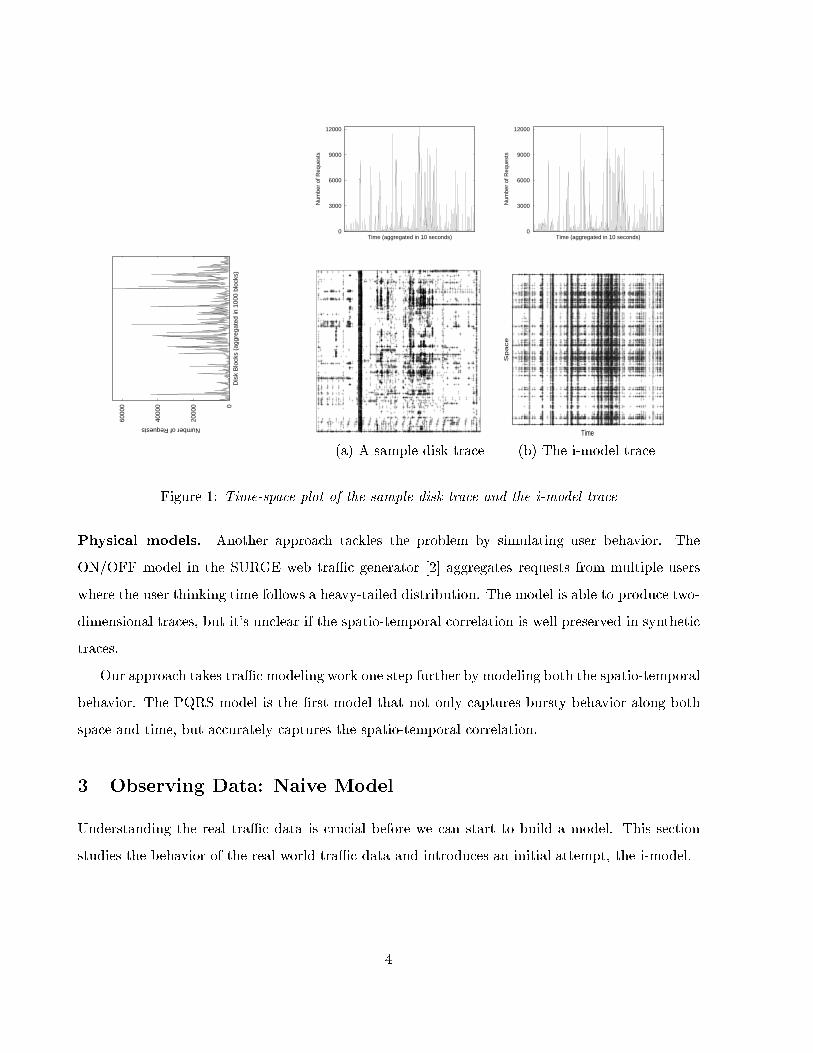
(a) A sample disk trace (b) The i-model trace

Figure 1: Time-space plot of the sample disk trace and the i-model trace

Physical models. Another approach tackles the problem by simulating user behavior. The

ON/OFF model in the SURGE web traÆc generator [2] aggregates requests from multiple users

where the user thinking time follows a heavy-tailed distribution. The model is able to produce two-

dimensional traces, but it's unclear if the spatio-temporal correlation is well preserved in synthetic

traces.

Our approach takes traÆc modeling work one step further by modeling both the spatio-temporal

behavior. The PQRS model is the �rst model that not only captures bursty behavior along both

space and time, but accurately captures the spatio-temporal correlation.

3 Observing Data: Naive Model

Understanding the real traÆc data is crucial before we can start to build a model. This section

studies the behavior of the real world traÆc data and introduces an initial attempt, the i-model.

4

3.1 Burstiness

De�ne the time-space plot as the projection of trace Y to the time space plane. Figure 1 shows

the time-space plot for the cello disk trace [13]. CT;S(t; s) is the number of tuples (t; s) in the

trace. That is, the number of requests of arrival time t of location s. Further projection of the

trace onto time and space gives the \marginal" one-dimensional traces CT and CS , in which CT (t)

and CS(s) tell the number of requests at time t or on block s. We observe \bursty" behavior (i.e.

non-uniformity) in both marginals.

� Temporal burstiness. The temporal burstiness is expected: various traÆc data, such as

disk I/O traÆc [10] and network traÆc [11, 7], have all been shown bursty.

� Spatial burstiness. CS is apparently not uniform, nor piece-wise uniform as some previous

work assumes. The spatial skewness has been noticed before [4], yet there is little e�orts on

modeling it. Existing one-dimensional models should be able to capture the spatial burstiness

in the same way as they do for the temporal burstiness since the bursty behavior looks similar

for time and space.

However, even if we do know both marginals, we can not generate two-dimensional traces if no

combining algorithm is available. The straight-forward combining algorithm is the i-model, which

is discussed in the next section.

3.2 I-Model

The i-model generates a two-dimensional trace by \multiplying" two marginal traces. For example,

if 10% of the total requests arrive between at time t and 5% of the total requests occur on disk

blocks on s, 10%� 5% of the total requests arrive at t on disk block number s.

Formally, the I-model speci�es that given CT and CS ,

CT;S(t; s) = CT (t)� CS(s)=M; t = 1; 2; : : : ; s = 1; 2; : : : ; (1)

where M is the total number of requests in the trace.

The i-model works with all one-dimensional models and preserves the temporal and spatial

burstiness because the marginals of the generated two-dimensional trace are exactly the same as

5

the original. In addition, it requires no parameters. Despite of numerous advantages, the i-model

ignores a very important property of the traÆc: strong spatio-temporal correlation. Figure 1 (b)

shows a two-dimensional trace generated by the i-model with CT and CS derived from the real

trace. We observe signi�cant di�erences between the i-model trace and the real one. The di�erence

is attribute to the existence of strong spatio-temporal correlation in the real trace. In fact, the

independence assumption leads to grossly pessimistic results, as we show in Section 6.

4 Proposed Method to Quantify Burstiness

The i-model contradicts the intuition that requests arriving closely in time tend to access nearby

objects. Thus, the correlation will have a great impact on the performance behavior because

requests to nearby objects take less time to serve. This section discusses how to measure the

correlation.

4.1 De�nitions

Various measures are proposed to measure the uniformity of a probability function, such as gini

index and entropy. We employ the entropy as our measurement in this paper. (The parameters

used in the paper along with their de�nitions are summarized in Table 1.)

Entropy is a well-known concept in information theory to measure the uniformity of a discrete

probability function [14]. Recall that entropy on a random variable E, (e.g. disk block id of

random requests), is de�ned as

H(E) = �NXi=0

pi log2 pi; (2)

where pi is the probability that event Ei will happen (e.g. the i-th block will be hit) and N is

the total number of possible outcomes (e.g. total number of disk blocks). H is close to 0 if the

distribution is highly skewed while a uniform distribution gives the maximum value of log2N for

H.

The joint entropy on two random variables is de�ned similarly: for a given probability function

P = fpi;jg on two random variables fEg and fFg, (e.g. arrival time and disk block id of random

requests), where pi;j gives the probability that both event Ei and event Fj will happen, (e.g. a disk

6

PT;S(t; s) Probability that a request on location s will arrive at time t.

PT (t) Probability that a request will arrive at time t.

PS(s) Probability that a request is on location s

H(E) Entropy of a random variable E

H(n)T Temporal entropy at aggregation level n

RT Slope of the temporal entropy plot

H(n)S Spatial entropy at aggregation level n

RS Slope of the spatial entropy plot

H(n)T;S Joint entropy on time and space at aggregation level n

RT;S Slope of the joint entropy plot

(p; q; r; s) Parameters to the PQRS model

M Total number of requests in a trace

Table 1: Symbols table.

request at block id j will arrive at i), the joint entropy on E and F is de�ned as

H(E;F ) = �Xi;j

pi;j log2 pi;j: (3)

De�nition 1 The mutual information I(E;F ) on two random variables E and F is de�ned as

I(E;F ) = H(E) +H(F )�H(E;F ): (4)

The mutual information I(E;F ) indicates the degree of correlation between E and F . It

becomes zero if E and F are independent.

4.2 Entropy Plots

We can apply the above de�nitions to traces to measure the burstiness and spatio-temporal cor-

relation. The question is, then, what the granularity should be. If we calculate the entropy on

the �nest resolution, the mutual information on time and space will be very close to zero because

no correlation will be observed. Our answer is to calculate the entropy values at all \aggregation"

levels.

To �nd the entropy values at aggregation level n, the trace is divided into 2n � 2n grids in the

time-space plot. Figure 2 (a) shows the grids at aggregation level n = 2. P(n)T;S is the probability

7

4

8

12

16

0 5 10 15

Ent

ropy

at a

ggre

gatio

n le

vel n

Aggregation level n

Entropy on timeEntropy on space

Joint entropy

(a) Aggregation level 2 (22 � 22

grids)(b) Entropy plots for the sample disktrace.

Figure 2: Entropy plot.

function that gives the probability that a request will fall into each grid, i.e. a request on location

(s1; s2) arriving at time (t1; t2). P(n)T and P

(n)S are the projections of P

(n)T;S on time and space and

can be easily derived from the given trace.

De�nition 2 At aggregation level n, de�ne the entropy on time, space and the joint entropy for a

given trace as 8>>>><>>>>:

H(n)T = H(P

(n)T );

H(n)S = H(P

(n)S );

H(n)T;S = H(P

(n)T;S):

(5)

Then, the entropy plots are the plots of the entropy values against the aggregation level n.

The entropy plot provides an insight on how the burstiness and correlation change across dif-

ferent resolution levels. The points form a line when the burstiness and correlation are stable

at di�erent granularities. Surprisingly, real traÆc shows stable burstiness and correlation over

aggregation as the linear entropy plots of the sample disk trace suggest (Figure 2 (b)).

Lemma 1 For a trace of stable temporal and spatial burstiness and spatio-temporal correlation, all

the entropy plots are linear: 8>>>><>>>>:

H(n)T = nRT ;

H(n)S = nRS;

H(n)T;S = nRT;S:

(6)

8

The intuition behind RT is the rate of information contained in one more bit of time-stamp.

� When all the requests come in a burst, all the time-stamps will be the same and the all the

bits are useless, which leads to RT = 0.

� When the requests are uniformly distributed along time, all the bits in the time-stamps are

useful and RT , in this case, is 1.

Similarly, RS gives the rate of information in the location bit. Denote RT +RS �RT;S as RI . RI

tells the mutual information per bit, e.g. how much information the time-stamp bit tells about the

location of the request.

� When RI equals to 0, the time-stamp and the location of a request is independent.

� The real traÆc data shows strong spatio-temporal correlation. The real trace in Figure 2 (b)

gives 0.722, 0.573, 0.881 as the estimated values for RT , RS , and RT;S. The calculated value

of RI turns out to be 0.414, indicating strong spatio-temporal correlation. The i-model trace,

on the other hand, render 0.001 for RI , which suggests independence between time and space.

(Hence the name i-model.)

5 Proposed Model: PQRS Model

The i-model fails to capture the spatio-temporal correlation in real traÆc. The following sections

present a new two-dimensional model, called the \PQRS" model, which has intrinsically stable

burstiness and correlation.

5.1 Generation: PQRS Model

The PQRS model generates a two-dimensional trace using four parameters, namely, p; q; r; s,

where p + q + r + s = 1. The recursive construction is the reverse process of the entropy plot

aggregation as illustrated in Figure 3 (a). At �rst, the probability that a request will fall into

the square is 1. In step 1, the time-space plot is divided into 2 � 2 grids and the probability

9

p*s

p*rp*p

p*q

qp

sr

1

(a) Generation of a PQRS model (b) A Sample PQRS trace

Figure 3: Recursive trace generation process for the PQRS model.

that a request falls in each grid is p; q; r; s respectively. In

step 2, each grid is further divided into 4 small grids and

the requests in the grid are distributed to the four small

grids with the same ratio, p; q; r; s. The process goes on

recursively until the required resolution on time and space

is achieved. Figure 3 (b) gives a sample trace generated

by the PQRSmodel with p; q; r; s of 0:2; 0:3; 0:4; 0:1. More

requests are located at bottom right corner since r has the

greatest value among the four parameters.

initialize the stack;push the whole trace onto the stack;while (stack is not empty) dopop a square from the stack;if required resolution is met, thenoutput the requests of the square;

else

divide the square into 2� 2 grids;distribute the requests to the

grids;push the four grids onto the stack;

Figure 4: PQRS trace generation

The above algorithm assumes the same order of p; q; r; s is used in all the levels. A random PQRS

trace can be generated by imposing a di�erent order at each step.

5.2 Parameter Fitting

The recursive construction algorithm guarantees that PQRS traces have linear entropy plots. The

burstiness and spatio-temporal correlation are stable because all the steps use the same parameters

to distribute the requests.

Lemma 2 Traces generated by the PQRS model have stable burstiness and correlation as they have

10

linear entropy plots. 8>>>><>>>>:

H(n)T = nH

(1)T ;

H(n)S = nH

(1)S ;

H(n)T;S = nH

(1)T;S;

(7)

Lemma 3 For a PQRS trace generated with parameter p; q; r; s, p+q+r+s = 1, the entropy rates

are 8>>>><>>>>:

RT = �(p+ q) log2(p+ q)� (r + s) log2(r + s);

RS = �(p+ r) log2(p+ r)� (q + s) log2(q + s);

RT;S = �p log2 p� q log2 q � r log2 r � s log2 s:

(8)

All the proofs are omitted from the paper for brevity. Equation 8 suggests that p + q determines

the temporal burstiness of the synthetic traces and p+ r determines the spatial burstiness. Given

the same temporal and spatial burstiness, varying the value of p changes the degree of the spatio-

temporal correlation.

The parameter �tting algorithm for the PQRS model is simple. For a given trace, plugging the

slopes of the entropy plots in Equation 8 gives the values for p; q; r; s.

The following two lemmas give some additional features of the PQRS model.

Lemma 4 The Poisson model is a special case of the PQRS model where p = q = r = s = 0:25.

Lemma 5 The i-model is a special case the PQRS model where pq= r

s.

5.3 Complexity

The computational complexity of the algorithm is an important property of the model. One would

rather choose to collect real traces if the trace generation is too slow. Ideally, the model should

o�er linear scalability. This section analyzes the computational complexity of the PQRS model.

Our analysis shows that both the trace generation and the parameter �tting algorithms o�er linear

scalability.

Lemma 6 The computation complexity for trace generation in the PQRS model is O(M � N),

where M is the total number of requests and N is the resolution level.

Proof: Omitted for brevity.

11

We outline the proof here. We upper-bound the trace generation through a naive implementation

of the algorithm. The recursive generation conceptually forms a quad tree. (See Figure 3 (a).)

The 4n grids in step n form the 4n nodes at level n in the quad tree. In the naive implementation,

we decide the value of t and s for a request (t; s) by walking down the quad tree from the root

to a leaf node. The probability that the request goes into the four subtrees is given by p; q; r; s.

Enumerating all the requests gives the �nal trace. The number of levels of the quad tree is bound by

O(N), where N is the number of steps involved. Therefore, the complexity of the trace generation

is O(M �N). In reality, N is usually the logarithm to the length of the trace in time (or space).

Similarly, the computation e�ort of the entropy plots scales linearly to the number of requests

as well.

Lemma 7 The computation complexity for parameter �tting algorithm of the PQRS model is

O(M �N).

Proof: Omitted for brevity.

We give a sketch of the proof here. For a given trace of M requests, the number of points in the

entropy plot is O(N). The number of non-zero grids in each step is less than M , thus, it takes

O(M) computations to generate a point in the entropy plot. Therefore, the total computational

complexity to compute the entropy plots is O(M �N):

In summary, the strength of the PQRS model lies in its power as well as in its simplicity.

The model generates traces with stable burstiness and correlation as the real traÆc data exhibits.

Additionally, the model o�ers linear scalability.

6 Experiments

We evaluate the PQRS model using both disk and memory reference traces. The experiments

examine the validity of the PQRS model and compares the performance behavior of the PQRS

model traces to the real ones.

We made two main observations. First, the real traÆc data have reasonably linear entropy

plots which veri�es the assumption we made in the PQRS model. Second, strong spatio-temporal

correlation plays an important role in performance behavior and invalidates the i-model. The PQRS

model, on the other hand, leads to performance measures that match reality.

12

6.1 Experiment Setup

Table 2 gives the summary of the disk I/O and memory traces in use.

Cello disk traces. The disk traces were collected on a UNIX �le server in HP on June 12th,

1992 [13]. The server has 8 disks attached to it. Total of six traces are in use: Disk-a for the

aggregation of all the disk requests, Disk-r for all the read requests, Disk-w for all the write

requests, and Disk-0, Disk-2, Disk-7 for individual disk 0, 2, 7. All the traces are one day long.

The other �ve disks are not studied because of the small volume of disk requests. The arrival time

is accurate up to microseconds. The disk block number ranges from 0 to more than 5,000,000.

TPC-C memory reference traces. The TPC-C memory traces were collected on a realistic

processor simulator running TPC-C workloads on Shore [3]. TPC-C [1] is an online transaction

processing (OLTP) benchmark modeling the order processing operations of a wholesale supplier.

There are total of six traces: �ve for �ve types of transactions and one for a mixture of di�erent

types of transactions. Only references to the heap area are studied here.

Evaluation tools. The ultimate goal of traÆc modeling is to facilitate system designs. Therefore,

we focus on the performance aspect of the traces. We use the response time and queue length

distributions for disk traces and the cache miss ratio for memory reference traces as our performance

metrics.

Methodology. We want to answer the following questions: (a) Does real traÆc have stable

burstiness and correlation over aggregation? The real traÆc should have linear entropy plots for

the PQRS model to work. (b) If so, how does the PQRS model perform in modeling them?

Ideally, the synthetic traces should have the same performance behavior as the real ones when the

parameters used in trace generation are derived from the real ones.

6.2 Model Checking

The PQRS model is designed for the traÆc data with stable burstiness and spatio-temporal corre-

lation. Therefore, the traÆc data should have linear entropy plots for the PQRS model to work.

13

At the same time, linear entropy plots give a good estimation for parameter p; q; r; s.

Figure 5 shows the entropy plots for the disk and memory traces. We have made the following

observations.

1. The entropy plots are reasonably linear, suggesting stable burstiness and correlation in the

traces. The estimated slopes are listed in Table 2. The stability ensures that the traces are

well within the capability of the PQRS model.

2. Strong spatio-temporal correlation exists in both types of traces. The mutual information

ranges from 0.313 to 0.696 for disk traces and from 0.166 to 0.417, indicating strong correla-

tion.

3. The PQRS model is able to model uniform traces as well. RT for the memory traces is close

to 1, suggesting a uniform distribution of the memory accesses on time. This is because the

program is consistently accessing data during its course of execution.

In summary, real traÆc data has stable burstiness and correlation over aggregation and is

within the capability of the PQRS model. Strong correlation exists, invalidating the independence

assumption of the i-model.

Table 2 gives the estimated p; q; r; s value from Equation (8) for the real traces. The following

sections compare the performance behavior of the real traces and the PQRS traces generated from

the estimated p; q; r; s value.

6.3 Disk Trace Evaluation

Figure 6 show the response time and queue length distributions of the real and the PQRS traces on

a realistic disk simulator [8]. Both distributions are in negative cumulative form and in log-scale.

That is, a point (10; 0:01) in the response time distribution plot says the more than 1% of the disk

requests have response time greater than 10 milliseconds. We expect that traces with strong spatio-

temporal correlation should have short tails in these distributions as requests close in location can

be served faster.

The comparison has shown that the PQRS traces, accurately capturing the burstiness and the

correlation, simulates the performance behavior of the real traces very well.

14

Trace Total disk requests RT RS RT;S IT;S (p; q; r; s)

Disk-a 4,575,798 0.641 0.819 1.058 0.402 (0.862,0.001,0.257,0.741)

Disk-r 1,822,781 0.847 0.833 0.984 0.696 (0.016,0.258,0.720,0.006)

Disk-w 3,300,628 0.641 0.728 0.992 0.377 (0.150.0.013,0.053,0.784)

Disk-0 1,101,416 0.814 0.690 0.941 0.563 (0.043,0.184,0.772,0.001)

Disk-2 1,396,649 0.790 0.723 0.904 0.609 (0.200,0.027,0.001,0.772)

Disk-7 371,320 0.722 0.573 0.881 0.414 (0.056,0.135,0.808,0.001)

(a) Cello disk trace summary

Trace Length Total requests RT RS RT;S IT;S (p; q; r; s)

New Order 14,990,636 4,000,000 0.962 0.200 0.996 0.166 (0.030,0.255,0.001,0.714)

Payment 17,242,172 4,573,044 0.963 0.281 1.042 0.202 (0.239,0.047,0.713,0.001)

Order Status 1,355,168 268,943 0.950 0.456 0.989 0.417 (0.095,0.185,0.001,0.722)

Delivery 525,100 129,388 0.957 0.439 0.987 0.409 (0.090,0.192,0.001,0.717)

Stock Level 14,453,440 3,613,360 0.974 0.349 1.052 0.271 (0.231,0.064,0.704,0.001)

Mix 12,268,876 4,000,000 0.983 0.309 0.990 0.302 (0.248,0.054,0.697,0.001)(b) TPC-C memory reference trace summary (Trace length in CPU cycles)

Table 2: Trace Summary

0

2

4

6

8

10

12

14

16

18

0 5 10 15 20

Tem

pora

l ent

ropy

at a

ggre

gatio

n le

vel n

Aggregation level n

Disk-aDisk-r

Disk-wDisk-0Disk-2Disk-7

0

2

4

6

8

10

12

14

0 2 4 6 8 10 12 14 16Spa

tial e

ntro

py a

t agg

rega

tion

leve

l n

Aggregation level n

Disk-aDisk-r

Disk-wDisk-0Disk-2Disk-7

02468

101214161820

0 2 4 6 8 10 12 14 16 18 20Join

t ent

ropy

at a

ggre

gatio

n le

vel n

Aggregation level n

Disk-aDisk-r

Disk-wDisk-0Disk-2Disk-7

(a) Entropy plots on time, space and the joint entropy plot (from left to right) for the disk traces.

0

5

10

15

20

0 5 10 15 20

Tem

pora

l Ent

ropy

at A

ggre

gatio

n Le

vel n

Aggregation Level n

New OrderPayment

Order StatusDelivery

Stock LevelTPC-C Mix

0

4

8

12

0 5 10 15 20 25Spa

tial E

ntro

py a

t Agg

rega

tion

Leve

l n

Aggregation Level n

New OrderPayment

Order StatusDelivery

Stock LevelTPC-C Mix

0

5

10

15

20

0 5 10 15 20Join

t Ent

ropy

at A

ggre

gatio

n Le

vel n

Aggregation Level n

New OrderPayment

Order StatusDelivery

Stock LevelTPC-C Mix

(a) Entropy plots on time, space and the joint entropy plot (from left to right) for the memory traces.

Figure 5: Entropy plots for the cello disk and TPC-C memory reference traces.

15

1e-05

0.0001

0.001

0.01

0.1

1

10 100 1000 10000

Pr(

Res

pons

e tim

e >

= x

)

Response time (in ms)

RealPQRS

I-model1e-05

0.0001

0.001

0.01

0.1

1

10 100 1000 10000

Pr(

Res

pons

e tim

e >

= x

)

Response time (in ms)

RealPQRS

0.0001

0.001

0.01

0.1

1

10 100 1000 10000

Pr(

Res

pons

e tim

e >

= x

)

Response time (in ms)

RealPQRS

I-model

Disk-0 Disk-2 Disk-7(a) Response time distribution in NCDF

1e-05

0.0001

0.001

0.01

0.1

1

10 100 1000 10000

Pr(

Que

ue le

ngth

>=

x)

Queue length

RealPQRS

I-model1e-06

1e-05

0.0001

0.001

0.01

0.1

1

10 100 1000 10000

Pr(

Que

ue le

ngth

)

Queue length

RealPQRS

0.0001

0.001

0.01

0.1

1

10 100 1000 10000

Pr(

Que

ue le

ngth

>=

x)

Queue length

RealPQRS

I-model

Disk-0 Disk-2 Disk-7(b) Queue length distribution in NCDF

Figure 6: Disk Trace Performance Evaluation. (I-model traces for disk-2 crashes due to queue

saturation.

1. Strong spatio-temporal correlation plays an important role in performance behavior of the

traces as we have expected. Traces with strong correlation yield shorter tails in both distri-

butions. The real traces and the i-model traces have exactly the same temporal and spatial

burstiness. However, the i-model traces produce extremely large response time because of

the independence assumption. The i-model results for Disk-2 are missing because the queue

becomes long enough to saturate the system.

2. The PQRS model works amazingly well in simulating the real traÆc behavior by accurately

capturing both the burstiness as well as the strong correlation at all aggregation levels.

The above comparison has shown that the PQRS model mimic the real disk I/O traÆc very

well in performance behavior.

16

6.4 Memory Trace Evaluation

Memory trace evaluation involves comparing the cache miss rates of the real traces to the PQRS

traces. Two facts justify our choice of using the cache miss rate to evaluate the performance

behavior. First, the miss rate is an important performance metric in computer architecture research.

Second, the cache miss rate re ects the spatio-temporal behavior of the trace. Memory references

on nearby locations have a better chance to be cache hits if they are close to each other in arrival

time. Therefore, strong spatio-temporal correlation leads to low cache miss rates.

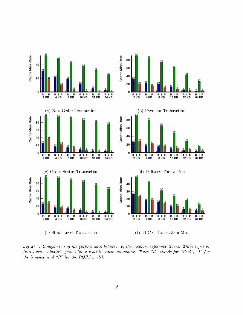
Figure 7 compares the cache miss rates for three sets of traces: R for the real traces; I for the

i-model traces generated from the same marginals as the real ones; P for the PQRS traces with

parameter values as listed in Table 2. Six groups of bars show the cache miss rates on six di�erent

cache sizes in each graph.

We observe that the traces with high degree of spatio-temporal correlation, such as the R and

P traces, su�er low cache miss rates as we have expected. The relative error of the PQRS traces

is within 30%. On the other hand, the I traces, assuming independence between time and space,

experience extremely high miss rates and have relative error as high as 1800%.

6.5 Summary

Both disk traces and memory references traces have shown reasonably stable burstiness and spatio-

temporal correlation over aggregation as suggested by the linear entropy plots. Strong correlation

between the arrival time and location of the requests exists in both types of traÆc data and it has

a signi�cant impact on the performance behavior of the traces. Therefore, traÆc modeling should

take spatio-temporal correlation into consideration.

The PQRS model, carefully designed for this type of traÆc data, is able to replicate the behavior

of real traces as shown by the experiments. The i-model, on the other hand, failed to do so by

ignoring the correlation.

7 Conclusions

Modeling disk traÆc is a hard problem [8], especially when we need to capture both the temporal

as well as spatial correlations. The contributions of this paper are the following:

17

| | | | | | | | ||0

|20

|40

Cac

he

Mis

s R

ate

R

31

I

54

P

19

2 KBR

22

I

48

P

10

4 KBR

19

I

43

P

4

8 KBR

12

I

38

P

1

16 KBR

5

I

32

P0

32 KBR

3

I

25

P0

64 KB

| | | | | | | | ||0

|20

|40

|60

|80

Cac

he

Mis

s R

ate

R

32

I

92

P

20

2 KBR

22

I

86

P

15

4 KBR

20

I

75

P

11

8 KBR

13

I

61

P

8

16 KBR

6

I

43

P

5

32 KBR

3

I

27

P

4

64 KB

(a) New Order Transaction (b) Payment Transaction

| | | | | | | | ||0

|20

|40

|60

|80

Cac

he

Mis

s R

ate

R

26

I

97

P

36

2 KBR

17

I

94

P

23

4 KBR

15

I

91

P

13

8 KBR

9

I

87

P

7

16 KBR

6

I

82

P

4

32 KBR

4

I

76

P

2

64 KB

| | | | | | | | ||0

|20

|40

|60

|80

Cac

he

Mis

s R

ate

R

27

I

89

P

30

2 KBR

18

I

80

P

23

4 KBR

16

I

67

P

16

8 KBR

10

I

49

P

11

16 KBR

6

I

30

P

8

32 KBR

5

I

14

P

6

64 KB

(c) Order Status Transaction (d) Delivery Transaction

| | | | | | | | ||0

|20|40

|60

|80

Cac

he

Mis

s R

ate

R

25

I

96

P

28

2 KBR

17

I

93

P

16

4 KBR

14

I

89

P

9

8 KBR

9

I

83

P

4

16 KBR

6

I

76

P

2

32 KBR

4

I

66

P1

64 KB

| | | | | | | | ||0

|10

|20

|30

|40

Cac

he

Mis

s R

ate

R

27

I

49

P

23

2 KBR

18

I

42

P

19

4 KBR

16

I

32

P

14

8 KBR

10

I

24

P

10

16 KBR

6

I

18

P

7

32 KBR

5

I

12

P

5

64 KB

(e) Stock Level Transaction (f) TPC-C Transaction Mix

Figure 7: Comparison of the performance behavior of the memory reference traces. Three types of

traces are evaluated against the a realistic cache simulator. Trace \R" stands for \Real"; \I" for

the i-model, and \P" for the PQRS model.

18

� we propose a simple model, the PQRS-model, that achieves all goals: it can be bursty or

uniform in time, bursty or uniform in space, and it can give zero to 100% correlation between

space and time.

� we propose a way to measure the spatio-temporal correlation, through the entropy plots and

the mutual information plots, which also showed that the burstiness and correlations remain

stable for many scales.

Smaller contributions include

� we are the �rst to quantify the popular, but vague intuition that memory and disk accesses

exhibit locality, not only in space or time, but in space-time as well.

� we give fast, scalable algorithms to build and run our model: They require linear time on the

number of requests M , to estimate the model parameters, and linear time again (O(M)) in

generating a trace of M requests.

� experiments on multiple real datasets show that the simple PQRS model can mimic them very

well, leading to good performance predictions (cache-hit-ratios, queue length distributions).

In contrast, the only other competitor, the independence model (i-model), fails miserably.

For example, the PQRS model traces have mean error 30% compared to the real traces while

the independence assumption can have error as high as 1800% in cache miss rates for the

memory traces.

One promising research direction could focus on the use of the PQRS model for other spatio-

temporal settings (e.g., earthquakes over space and time). Another direction could be the analytical

derivation of performance measures of interest (like the cache-hit ratio, or disk queue length distri-

butions), given the p; q; r; s values of a trace.

Acknowledgement We wish to thank John Wilkes from HP Storage System Lab for providing

us with the cello disk trace and constant feedback on our work. We are grateful to Jiri Schindler

for helping on the disk simulator. In particular, we appreciate Prof. Anthony Brockwell for his

insight on classical statistical models.

19

References

[1] TPC-C benchmark speci�cation. http://www.tpc.org/.

[2] Paul Bardord and Mark Crovella. Generating representative web workloads for network and server

performance evaluation. In SIGMETRICS'98, pages 151{160, 1998.

[3] M. Carey, D. J. DeWitt, M. Franklin, N. Hall, M. McAuli�e, J. Naughton, D. Schuh, M. Solomon,

C. Tan, O. Tsatalos, S. White, and M. Zwilling. Shoring up persistent applications. In SIGMOD, 1994.

[4] Stavros Christodoulakis. Implications of certain assumptions in database performance evaluation. ACM

Transactions on Database Systems, 9(2):163{186, 1984.

[5] David R. Cox and Valerie Isham. Point processes. Chapman and Hall, 1980.

[6] Noel A. C. Cressie. Statistics for spatial data. J. Wiley, 1991.

[7] Mark E. Crovella and Azer Bestavros. Self-similarity in world wide web traÆc evidence and possible

causes. In Proc. of the 1996 ACM SIGMETRICS Intl. Conf. on Measurement and Modeling of Computer

Systems, May 1996.

[8] Gregory R. Ganger. Generating representative synthetic workloads: An unsolved problem. In Proceed-

ings of the Computer Measurement Group (CMG) Conference, 1995.

[9] Mark W. Garrett and Walter Willinger. Analysis, modeling and generation of self-similar VBR video

traÆc. In SIGCOMM'94, 1994.

[10] Mar�ia E. G�omez and Vicente Santonja. Self-similiarity in I/O workload: Analysis and modeling. In

Workshop on Workload Characterization, 1998.

[11] W. E. Leland, M. S. Taqqu, W. Willinger, and D. V. Wilson. On the self-similar nature of ethernet

traÆc (extended version). IEEE Transactions on Networking, pages 1{15, 1994.

[12] Ruldolf H. Riedi, Matthew S. Crouse, Vinay J. Ribeiro, and Richard G. Baraniuk. A multifractal wavelet

model with application to network traÆc. In IEEE Transactions on Information Theory, number 3,

April 1999.

[13] Chris Ruemmler and John Wilkes. Unix disk access patterns. In Proceedings of the Winter'93 USENIX

Conference, pages 405{420, 1993.

[14] Claude E. Shannon and Warren Weaver. Mathematical Theory of Communication. University of Illinois

Press, 1963.

[15] Elizabeth Shriver, Arif Merchant, and John Wilkes. An analytic behavior model for disk drives with

readahead caches and request reordering. In SIGMETRICS'98, 1998.

[16] Mengzhi Wang, Tara Madhyastha, Ngai Hang Chan, Spiros Papadimitriou, and Christos Faloutsos.

Data mining meets performance evaluation: Fast algorithm for modeling bursty traÆc. In ICDE'02,

2002.

20