Embed Size (px)
Citation preview

OXYGEN DELIVERING PROCESSES IN GROUNDWATER AND THEIR
RELEVANCE FOR IRON-RELATED WELL CLOGGING PROCESSES– A
CASE STUDY ON THE QUATERNARY AQUIFERS OF BERLIN
Dissertation
zur Erlangung des akademischen Grades Dr. rer. nat.
eingereicht am Fachbereich Geowissenschaften
der Freien Universität Berlin
vorgelegt von
Christian Menz
aus Friedberg/Hessen
2016


3
1. Gutachter: Prof. Dr. Michael Schneider
2. Gutachter: Priv.-Doz. Dr. Christoph Merz
Disputation am 06.07.2016


5
Summary
Redox condition, in particular the amount of oxygen in groundwater used for drinking water supply, is a key factor for the drinking water quality as well as for the production well’s lifecycle. Thus, a process-based and quantitative understanding about the oxygen fluxes in groundwater systems is fundamental in order to predict e.g. the removal capacity of pollutants or in particular the likelihood of iron-related well clogging. Such well ageing is a major thread for well operators and objective in practice and science.
The formation of iron oxides responsible for well clogging is mainly known for wells abstracting groundwater from unconsolidated aquifers with a distinct redox zonation. The accumulation of precipitates is primarily taking place at the slots of the well screens, but also affects aquifers, pumps and collector pipes. Several studies already identified interacting hydro-chemical and microbiological processes as major cause for the development of iron oxides in wells. They develop in the presence of dissolved species of iron and oxygen in the water. The co-occurrence of both, the dissolved iron and oxygen, is the result of a mixing of groundwater with different redox states. The abstraction of groundwater by wells is known to promote such mixing processes. Particularly, frequent water table oscillations with high amplitudes in contrast to natural conditions and managed aquifer recharge measures may deliver oxygen to groundwater. But the impact of different well management strategies on the sources and rates of oxygen delivery to aquifers was not studied in detail so far.
Within the thesis presented here, oxygen fluxes to groundwater were qualified and quantified based on statistical, modelling, laboratory and field site studies and their impact on well performance was determined for different well operation schemes and different hydrogeological conditions. Processes were exemplarily investigated for the quaternary aquifers of Berlin, which are the exclusive source for the drinking water supply of the German capital. Analysis of design, operation, geological setting, hydro-chemical composition and maintenance activities of Berlin’s drinking water wells illustrated the vulnerability of wells for clogging processes and revealed the relevance of detailed investigations on this topic.
A general estimation of the two main oxygen delivering processes influencing groundwater aeration, air entrapment and bank filtration, was done by a generic transport model. Simulation of oxygen fluxes with regard to different hydrogeological and operational boundary conditions revealed air entrapment as major source. Oxygen delivery by bank filtration was subsidiary and strongly depending on flow gradients and permeability of the banks. Air entrapment due to oscillating water tables was quantified by aeration tests in column experiments under laboratory conditions. Results pointed at a downward shift of oxygen caused by repeated oscillations as a consequence of oxygen dissolution and advective transport of dissolved oxygen inside the column. A downward propagation of oxygen into the permanently water-saturated zone was not observed for switching intervals shorter than 24 hours. Such repeated short-termed oscillations led to an enrichment of oxygen, but with a constantly decreasing increment per oscillation.
Oxygen degradation was not accounted for in simulation and inhibited in laboratory studies. But, in situ monitoring of oxygen at three selected well sites in Berlin provided a real insight into oxygen fluxes and their effects on well ageing processes under field conditions. The monitoring network included multi-level observation wells and vertical strings of oxygen sensors installed in the aquifer and inside the wells. Thus, it was feasible to measure changes in hydraulic conditions and redox dynamics. Oxygen distribution could be observed as a function of depth and recharge source in a high temporal and spatial resolution for the first time. It was possible to detect traces of oxygen in the well-near aquifer and inside the wells, which are sufficient to oxidize high loads of dissolved iron when supplied constantly. All three well sites showed oxygen

6
distribution patterns, which significantly differed from the others. These variations referred not only to the initial distribution, sampled at idle equilibrium, but also to the progression of oxygen saturation during abstraction and recovery phases. Enrichment and downward propagation of oxygen as result of abstracting water could be observed at all well sites, although absolute concentrations varied strongly between the well sites. By this, it was possible to correlate oxygen variations to hydrogeological boundary conditions. Infiltrating oxic surface water via river, lake or artificial pond banks delivers high amounts of oxygen to the groundwater and can cause an enormous widening of the oxic zone towards the abstracting well. As a result, the oxic/anoxic interface moves downward close to the well once water is abstracted. But, clogging of wells abstracting bank filtrate or artificial recharge strongly depends on the residence times of the filtrate, the hydraulic connection between banks and groundwater and seasonal variations. Only under certain conditions a significant enhancement of clogging can be expected.
To directly link well operation, oxygen delivery and ochre formation with well performance development, a well model scaled up to realistic proportions was designed, built and operated with natural groundwater. The tank experiment enabled to study distribution patterns of ochre formation with regard to the different structural zones of the well, including aquifer, filter pack and screen slots and its influence on pressure losses and well performance. It could be shown, that groundwater was enriched with oxygen during the tank passage by oscillating water tables and that permeability and specific well yield generally decreased over time. The distribution of ochre deposits in the well tank showed a distinct mineral zonation with high deposition rates of manganese and iron in the filter pack at the top of the well screen. Further, interfaces of aquifer and/or filter pack were strongly affected by iron deposits.
Thus, preventing ochre formation is an appropriate measure. The preventive treatment of wells with hydrogen peroxide could be such a measure, but could also be a potential source for oxygen in well and filter pack. By reviewing the latest research activities and operator’s data and by investigating at laboratory and field site scale, the current treatment procedure was evaluated. Investigations revealed a clear improvement potential for the treatment with hydrogen peroxide. Impacts of the treatment were however low, especially if incrustations were already established. Results of column batch studies and field tests did not fully prove the effectiveness of the preventive treatment, but indicated that with higher concentrated solutions and an improved treatment procedure ochre formation can be retarded and rehabilitation potential can be improved.
Another approach to prevent ochre formation is the classification of well sites considering their ageing vulnerability and the development of adapted operation schedules. At least such a measure can support a sustainable construction, operation and maintenance of wells. A statistical approach was used to quantify well ageing and to identify factors promoting well performance loss. Most appropriate clogging indicators could be identified and were used to analyse worst and best site conditions with regard to their impact on ochre formation. Accordingly, a well in high distance to the next surface water with a thick groundwater layer above the well screen situated in a confined aquifer with high redox potential gains the lowest ageing potential. Compared to worst site conditions and calculated for the mean life time of a typical Berlin drinking water well, this can account for a difference in well capacity of up to 90%. In addition to that, optimized rehabilitation intervals for the identified well classes based on their ageing potential could be exemplarily determined.
Based on the results of this thesis, strategies for an optimized monitoring of well ageing processes and strategies for an adapted well management aiming at the reduction of ochre formation can be developed.
7
Zusammenfassung
Die Redoxbedingungen und insbesondere der Sauerstoffgehalt im Grundwasser haben nicht nur einen wesentlichen Einfluss auf die Qualität des daraus gewonnenen Trinkwassers, sie beeinflussen auch in erheblichem Maße die Leistungsfähigkeit und Lebenserwartung der Förderbrunnen. Daher ist ein prozessbasiertes Verständnis und eine quantitative Analyse der in Grundwasserleitern stattfindenden Sauerstoffströme grundlegend, um neben dem Rückhalt von Schadstoffen, auch die Wahrscheinlichkeit von Brunnenalterungsprozessen zu ermitteln und vorherzusagen. Gerade die Brunnenalterung ist für die Betreiber von Brunnenanlagen ein zentrales Thema und deshalb von großer Bedeutung für Praxis und Forschung.
Unlösliche Eisenverbindungen, auch bekannt als Verockerung, vermindern durch ihre Ablagerung in den Brunnenfiltern, aber auch im angrenzenden Grundwasserleiter, die Produktivität der Brunnen in erheblichem Maße. Die notwendige Instandhaltung und der Neubau von Brunnenanlagen verursachen erhebliche Kosten für die Betreiber. Produktivitätsabnahmen durch Verockerungen werden hauptsächlich bei solchen Brunnen beobachtet, die Grundwasser aus Grundwasserleitern mit einer ausgeprägten Redoxzonierung fördern. Mehrere wissenschaftliche Studien haben bereits ein Zusammenspiel von hydrochemischen und mikrobiologischen Prozessen als Hauptursache für die Entstehung von Eisenausfällungen in Brunnen identifiziert. Diese bilden sich, sobald Sauerstoff und Eisen in gelöster Form im Wasser vorhanden sind. Beide Stoffe treten gemeinsam im Wasser auf, wenn sich Grundwässer mit unterschiedlichen Redoxbedingungen mischen. Es ist nachgewiesen, dass die Entnahme von Grundwasser mittels Brunnen solche Mischungsprozesse verstärkt auftreten lässt. Insbesondere häufige und ausgeprägte Schwankungen der Grundwasseroberfläche und Maßnahmen zur künstlichen Grundwasseranreicherung können größere Mengen an Sauerstoff ins Grundwasser eintragen. Die Auswirkungen unterschiedlicher Grundwasserbewirtschaftungsstrategien auf die Quellen und den Transport von Sauerstoff im Grundwasser wurden jedoch bisher nicht explizit betrachtet.
In der hier vorgestellten Arbeit werden die Sauerstoffströme ausgehend von statistischen, modellbasierten und labortechnischen Verfahren sowie im Geländemaßstab beschrieben und quantifiziert. Die Bedeutung der Sauerstoffströme für die Leistungsentwicklung von Brunnen wird basierend auf den Ergebnissen für verschiedene Bewirtschaftungsszenarien und verschiedene hydrogeologische Randbedingungen bewertet. Die Prozesse wurden beispielhaft für die quartären Grundwasserleiter Berlins untersucht. Diese bilden die wichtigste Trinkwasserressource für die Bundeshauptstadt. Die Analyse von Stamm- und Betriebsdaten der Brunnen, sowie von Instandhaltungsdaten zeigt die Anfälligkeit der Brunnen für Alterungsprozesse und verdeutlicht wie wichtig detailliertere Untersuchungen zu diesem Thema sind.
Um die Auswirkungen der beiden wichtigsten Eintragspfade von Sauerstoff, Lufteintrag durch Schwankungen der Wasseroberfläche und Uferfiltration abzuschätzen, wurde ein generisches Transportmodell erstellt. Durch die für beide Eintragspfade unter verschiedenen hydraulischen Randbedingungen berechneten Sauerstoffströme konnte der Eintrag über Wasserstandschwankungen als dominanter Prozess identifiziert werden. Der Eintrag von Sauerstoff über Uferfiltration war nachrangig und stark von den hydraulischen Randbedingungen bei der Infiltration abhängig. Zur Quantifizierung der Sauerstoffmengen, die durch schwankende Grundwasseroberflächen ins Grundwasser eingetragen werden, wurden Belüftungsversuche an Säulen mit sauerstofffreiem Wasser durchgeführt. Die Ergebnisse zeigten, dass sich Luftsauerstoff durch wiederholte Schwankungen im Wasser löste und advektiv in der Säule nach unten transportiert wurde. Es konnte jedoch nicht beobachtet werden, dass Sauerstoff sukzessive im permanent wassergesättigten Bereich der Säule angereichert wurde, solange die Schwankungsintervalle kürzer als ein Tag waren. Diese kurzzeitigen Schwankungen

8
führten lediglich zu einer kontinuierlichen Sauerstoffanreicherung in der Schwankungszone.
Die unter natürlichen Bedingungen stattfindende Sauerstoffzehrung spielt eine wichtige Rolle bei der Sauerstoffverteilung im Grundwasser. Sie wurde bei der Simulation jedoch nicht berücksichtigt und in den Laborversuchen gezielt unterdrückt. Deshalb sollten in situ-Messungen von Sauerstoff an drei ausgewählten Brunnenstandorten in Berlin einen Einblick in die natürlichen Sauerstoffströme und deren Auswirkungen auf Brunnenalterungsprozesse geben. Mehrfachmessstellen und Sauerstoffsonden sollten in unterschiedlichen Tiefen im Grundwasserleiter und im Brunnen Änderungen in Hydraulik und Redoxverhalten erfassen. So konnte zum ersten Mal die Sauerstoffverteilung in hoher zeitlicher und räumlicher Auflösung beobachtet werden. Es konnten Spurenkonzentrationen von Sauerstoff sowohl im Grundwasser als auch im Brunnen nachgewiesen werden, die bei konstantem Auftreten ausreichend wären um auch höhere Konzentrationen von im Wasser gelösten Eisen zu oxidieren. Dabei unterschieden sich alle drei untersuchten Brunnenstandorte deutlich in ihrer Sauerstoffverteilung. Diese Unterschiede zeigten sich nicht nur im Ruhezustand zu Beginn der Versuche sondern auch im weiteren Verlauf während der verschiedenen Betriebsphasen. An allen drei Standorten konnte mit beginnender Grundwasserförderung eine Verlagerung des oberflächennahen Sauerstoffs in die Tiefe beobachtet werden. Die Höhe der Sauerstoffkonzentrationen waren jedoch sehr standortabhängig, was Korrelationen zwischen den Sauerstoffströmen und den hydrogeologischen Randbedingungen ermöglichte. Hohe Sauerstoffgehalte im Grundwasser konnten infiltrierendem sauerstoffreichem Oberflächenwasser zugeordnet werden und führten zu einer erheblichen Vergrößerung der oxischen Zone rund um den Brunnen. Die Entstehung von Eisenablagerungen hängt bei diesen Brunnen im Wesentlichen von den Fließzeiten des Filtrats, von der hydraulischen Anbindung der Uferbereiche an das Grundwasser und von saisonalen Effekten ab. Nur unter bestimmten Ausgangsbedingungen trat eine signifikant stärkere Verockerung dieser Brunnen auf.
Um die tatsächlich vorhandene Auswirkung des Sauerstoffeintrages auf die Entstehung von Eisenausfällungen zu untersuchen, wurde ein real-skaliertes Brunnenmodell konstruiert und mit natürlichem Grundwasser durchströmt. Diese Versuchsanordnung ermöglichte es, die Verteilung der Eisenausfällungen den verschiedenen Brunnenelementen zuzuordnen und deren Einfluss auf die Entwicklung von Druckverlusten und Brunnenleistung zu ermitteln. Es konnte gezeigt werden, dass das Grundwasser während der Modellpassage durch Brunnenschaltungen über Lufteinschlüsse mit Sauerstoff angereichert wurde und sowohl die hydraulische Durchlässigkeit, als auch die spezifische Brunnenergiebigkeit über die Zeit abnahmen. Die entstandenen Mineralausfällungen traten dabei vermehrt in der Filterschüttung und dort im Bereich der Filteroberkante auf. Hier war zudem eine Zonierung von Mangan- und Eisenverbindungen zu erkennen. Des Weiteren waren die Übergangsbereiche von Grundwasserleiter zu äußerer und äußerer zu innerer Filterschüttung stark von Eisenablagerungen betroffen.
Zur Verhinderung von Eisenausfällungen können sich präventive Maßnahmen als wirksam darstellen. Die Behandlung von Brunnen mit Wasserstoffperoxid könnte eine solche präventive Maßnahme sein. Sie könnte aber auch eine zusätzliche Quelle für Sauerstoff in Brunnen und Filterschüttung darstellen. Die bereits bestehende und von den Berliner
Wasserbetrieben angewandte Behandlung wurde deshalb anhand des aktuellsten Forschungsstands, der Brunnenbetriebsdaten und anhand von Labor- und Felduntersuchungen überprüft und bewertet. Im Ergebnis zeigte sich ein deutliches Optimierungspotential. So sind die Auswirkungen der Behandlung generell nur gering, insbesondere wenn sich bereits Eisenablagerungen im Brunnen etabliert haben. Auch die durchgeführten Versuche konnten die Effektivität der Behandlung nicht gänzlich nachweisen, deuteten jedoch Effektivitätssteigerungen bei der Verwendung höher konzentrierter Wasserstoffperoxidlösungen bei veränderter Behandlungsprozedur an. Den Ergebnissen zufolge hatte die präventive Behandlung vor allem einen positiven Effekt auf die Regenerierbarkeit der Brunnen.

9
Ein weiterer Ansatz Eisenablagerungen erst gar nicht entstehen zu lassen, ist die Klassifizierung von Brunnen entsprechend ihres Alterungspotentials und die Entwicklung von spezifischen Betriebsregimen. Diese Maßnahme kann auch einen nachhaltigen Bau und Betrieb sowie eine optimierte Instandhaltung der Brunnen unterstützen. Es wurde ein statistischer Ansatz gewählt um die Brunnenalterung zu quantifizieren und um die Faktoren zu identifizieren, die hauptverantwortlich für die Leistungsverluste sind. Die ermittelten Faktoren wurden verwendet um die günstigsten, beziehungsweise ungünstigsten Randbedingungen für Brunnenalterungsprozesse darzustellen. Demzufolge besitzt ein Brunnen, der (i) in großem Abstand zu einem Oberflächengewässer liegt und (ii) Wasser mit einem hohen Redoxpotential (iii) aus einem bedeckt-gespannten Grundwasserleiter (iv) mit einer mächtigen Grundwasserüberdeckung fördert das geringste Alterungspotential. Verglichen mit den ungünstigsten Randbedingungen und bezogen auf die durchschnittliche Lebensdauer eines Berliner Trinkwasserbrunnens kann dies einen Unterschied in der Ergiebigkeit von bis zu 90 % ausmachen. Darüber hinaus konnten für die ermittelten Brunnenklassen entsprechend ihres Alterungspotentials optimierte Instandhaltungszyklen berechnet werden.
Basierend auf den Ergebnissen dieser Arbeit, können neue Strategien für eine optimierte Überwachung der Brunnenalterungsprozesse und Strategien für einen angepassten Brunnenbetrieb mit dem Ziel die Eisenablagerungen zu minimieren, entwickelt werden.


11
Table of Contents
SUMMARY ....................................................................................................................... 5
ZUSAMMENFASSUNG ........................................................................................................ 7
TABLE OF CONTENTS ...................................................................................................... 11
LIST OF FIGURES............................................................................................................ 15
LIST OF TABLES .............................................................................................................. 19
GENERAL INTRODUCTION ............................................................................ 21 CHAPTER 1
BACKGROUND ...................................................................................................... 21 1.1
TASK AND OBJECTIVE ........................................................................................... 21 1.2 STUDY AREA......................................................................................................... 22 1.3
HYDROGEOLOGY ............................................................................................. 22 1.3.1 WATER SUPPLY .............................................................................................. 25 1.3.2
OXYGEN IN GROUNDWATER ................................................................................... 26 1.4 OXYGEN DELIVERY BY AIR ENTRAPMENT AND BUBBLE-MEDIATED TRANSPORT ......................... 26 1.4.1
OXYGEN DELIVERY BY INFILTRATING SURFACE WATER ................................................... 27 1.4.2
WELL AGEING ....................................................................................................... 29 1.5 WELL CLOGGING BY IRON HYDROXIDE .................................................................... 30 1.5.1 IMPACT OF WELL AGEING ON WELL MANAGEMENT ISSUES ............................................... 32 1.5.2
OUTLINE OF THE THESIS ....................................................................................... 33 1.6
CHARACTERIZATION OF BERLIN WELL SITES WITH REGARD TO OCHRE CHAPTER 2
FORMATION .................................................................................................. 35
INTRODUCTION .................................................................................................... 35 2.1 METHODS AND MATERIALS .................................................................................... 36 2.2
RESULTS .............................................................................................................. 37 2.3
WELL AGE .................................................................................................... 37 2.3.1
AQUIFER TYPE ............................................................................................... 38 2.3.2 WELL DESIGN AND LOCATION .............................................................................. 38 2.3.3 WELL OPERATION ........................................................................................... 39 2.3.4 REHABILITATION INTERVALS ............................................................................... 40 2.3.5
HYDROCHEMISTRY IN GENERAL ............................................................................ 41 2.3.6
EVALUATION OF REDOX SENSITIVE PARAMETER ...................................................... 43 2.4 METHODS .................................................................................................... 43 2.4.1 RESULTS ..................................................................................................... 44 2.4.2
CONCLUSIONS...................................................................................................... 45 2.5
SIMULATION OF OXYGEN TRANSPORT TOWARDS A DRINKING WATER WELLCHAPTER 3
..................................................................................................................... 47
INTRODUCTION .................................................................................................... 47 3.1 METHODS ............................................................................................................ 48 3.2
HYDROGEOLOGICAL SETTING AND CONCEPTUAL MODEL ................................................. 48 3.2.1 MODEL DESIGN .............................................................................................. 49 3.2.2 SCENARIOS .................................................................................................. 51 3.2.3
RESULTS .............................................................................................................. 52 3.3
IMPACT OF DIFFERENT HYDROGEOLOGICAL CONDITIONS ON THE OXYGEN DELIVERY ................. 52 3.3.1 IMPACT OF SOURCE TYPE ON OXYGEN CONCENTRATIONS IN THE WELL ................................. 57 3.3.2
CONCLUSIONS...................................................................................................... 57 3.4
12
QUANTIFYING AIR ENTRAPMENT AND OXYGEN UPTAKE FROM OSCILLATING CHAPTER 4
WATER TABLES IN COLUMN EXPERIMENTS ................................................... 59
INTRODUCTION .................................................................................................... 59 4.1 METHODS AND MATERIALS .................................................................................... 60 4.2
COLUMN SETUP .............................................................................................. 60 4.2.1 BULK MATERIAL.............................................................................................. 61 4.2.2
EXPERIMENT DESIGN ........................................................................................ 62 4.2.3 RESULTS .............................................................................................................. 63 4.3
OXYGEN DELIVERY DEPENDENT ON OSCILLATION AMPLITUDE ........................................... 63 4.3.1
OXYGEN DELIVERY DEPENDED ON OSCILLATION FREQUENCY ............................................ 64 4.3.2 TIME-DEPENDENT OXYGEN SATURATION DURING DRAWDOWN AND RECOVERY ........................ 66 4.3.3
CONCLUSIONS...................................................................................................... 67 4.4
IMPACT OF WATER ABSTRACTION ON THE SOURCE AND DISTRIBUTION OF CHAPTER 5
DISSOLVED OXYGEN IN WELLS – A FIELD SITE STUDY ................................. 69
INTRODUCTION .................................................................................................... 69 5.1 STUDY SITES ........................................................................................................ 70 5.2
SELECTION OF TEST SITES ................................................................................. 70 5.2.1 TEST SITE WELL 15 ........................................................................................ 72 5.2.2 TEST SITE WELL 18 ......................................................................................... 74 5.2.3 TEST SITE WELL 22 ......................................................................................... 76 5.2.1
METHODS AND MATERIALS .................................................................................... 78 5.3
EXPERIMENTAL DESIGN ..................................................................................... 78 5.3.1 MONITORING NETWORK DESIGN ........................................................................... 80 5.3.2 MONITORED PARAMETER.................................................................................... 81 5.3.3
IMPACT OF WELL SWITCHING EVENTS .................................................................... 83 5.4 RESULTS AND DISCUSSION ................................................................................. 83 5.4.1
CONCLUSIONS ............................................................................................... 89 5.4.2
IMPACT OF CONTINUOUS WELL OPERATION............................................................. 91 5.5 RESULTS AND DISCUSSION ................................................................................. 91 5.5.1
CONCLUSIONS ............................................................................................... 97 5.5.2 IMPACT OF WELL INTERFERENCES .......................................................................... 99 5.6
RESULTS AND DISCUSSION ................................................................................. 99 5.6.1 CONCLUSIONS ............................................................................................. 104 5.6.2
ESTIMATION AND COMPARISON OF OXYGEN DELIVERY RATES ................................. 105 5.7 OXYGEN DELIVERY BY WATER LEVEL OSCILLATION ..................................................... 105 5.7.1
OXYGEN DELIVERY BY BANK FILTRATE ................................................................... 106 5.7.2 IMPLICATIONS FOR WELL CLOGGING PROCESSES .................................................. 108 5.8
CONCLUSIONS.................................................................................................... 110 5.9
OXYGEN DEPENDENCY OF IRON-RELATED WELL CLOGGING PROCESSES – A CHAPTER 6
HYDRAULIC, HYDROCHEMICAL AND GEOCHEMICAL WELL MODEL STUDY ... 113
INTRODUCTION .................................................................................................. 113 6.1
METHODS .......................................................................................................... 114 6.2 MODEL WELL DESIGN ..................................................................................... 114 6.2.1 MONITORING DESIGN ..................................................................................... 116 6.2.2
EXPERIMENT DESIGN ...................................................................................... 117 6.2.3 RESULTS AND DISCUSSION ................................................................................. 118 6.3
CONSTANT FLOW CONDITIONS ........................................................................... 118 6.3.1 STAGNANT FLOW CONDITIONS ........................................................................... 119 6.3.2
TRANSIENT FLOW CONDITIONS .......................................................................... 119 6.3.3 OCHRE DEPOSITION ....................................................................................... 123 6.3.4
CONCLUSIONS.................................................................................................... 126 6.4

13
THE PREVENTIVE TREATMENT OF WELLS WITH HYDROGEN PEROXIDE – A CHAPTER 7
POTENTIAL OXYGEN SOURCE FOR IRON CLOGGING OR AN EFFECTIVE ANTI-
AGING MEASURE ......................................................................................... 129
INTRODUCTION .................................................................................................. 129 7.1
PRELIMINARY TESTS ........................................................................................... 130 7.2 DECOMPOSITION OF HYDROGEN PEROXIDE ............................................................. 130 7.2.1
IMPACT ON WELL YIELD ................................................................................... 132 7.2.2 METHODS .......................................................................................................... 132 7.3
BATCH TESTS ON TREATMENT FREQUENCY AND SOLUTION CONCENTRATION ........................ 133 7.3.1
FIELD SITE TESTS ON TREATMENT PROCEDURE ......................................................... 133 7.3.2 RESULTS ............................................................................................................ 134 7.4
BATCH TESTS ON TREATMENT FREQUENCY AND SOLUTION CONCENTRATION ........................ 134 7.4.1 FIELD SITE TESTS ON TREATMENT PROCEDURE ......................................................... 135 7.4.2 VALIDATION OF RESULTS AND RECOMMENDATION FOR AN IMPROVED TREATMENT PROCEDURE .... 136 7.4.3
CONCLUSIONS.................................................................................................... 138 7.5
QUANTITATIVE ANALYSIS OF IRON-RELATED WELL AGEING POTENTIAL .. 139 CHAPTER 8
INTRODUCTION .................................................................................................. 139 8.1 IDENTIFICATION OF CLOGGING FACTORS ............................................................. 140 8.2
METHODS AND MATERIALS ............................................................................... 140 8.2.1 RESULTS ................................................................................................... 141 8.2.2
QUANTITATIVE ANALYSIS .................................................................................... 145 8.3
METHODS AND MATERIALS ............................................................................... 145 8.3.1 RESULTS ................................................................................................... 147 8.3.2
CONCLUSIONS.................................................................................................... 150 8.4
SYNTHESIS ................................................................................................ 153 CHAPTER 9
SOURCES AND EFFECTS OF OXYGEN IN WELL OPERATION ....................................... 153 9.1
OXYGEN DELIVERY BY BANK FILTRATION ................................................................ 153 9.1.1 OXYGEN DELIVERY BY AIR ENTRAPMENT ................................................................. 153 9.1.2 EFFECT OF THE WELL FIELD-RELATED POSITION ........................................................ 155 9.1.3
DIAGNOSIS OF OCHRE FORMATION PROCESSES .................................................... 156 9.2 REDUCTION OF SPECIFIC WELL YIELD ................................................................... 156 9.2.1
WELL LOSS DEVELOPMENT ............................................................................... 156 9.2.2 INFLOW ZONES ............................................................................................ 157 9.2.3 DEPOSIT DISTRIBUTION .................................................................................. 157 9.2.4
ADAPTED STRATEGIES FOR WELL OPERATION ........................................................ 158 9.3
REFERENCES ............................................................................................ 161 CHAPTER 10
APPENDIX A ................................................................................................................. 169
PUBLICATIONS ............................................................................................................. 183
ACKNOWLEDGEMENT .................................................................................................... 185


15
List of Figures
Fig. 1.1: Possible mixing processes of O2- and Fe(II)-bearing water in aquifers and wells induced by well operation. A: Horizontal mixing of oxic bank filtrate with anoxic groundwater. B: Vertical mixing of re-aerated shallow groundwater with anoxic deep groundwater. C: Mixing due to hydraulic interference between neighbored wells ........................................................... 22
Fig. 1.2: Schematic map of the occurring Cenozoic formations, on the Berlin surface after KLOOS (1986). .................................................................................................................... 23
Fig. 1.3: Schematic hydrogeological cross-section from the north to the south of Berlin (Limberg & Thierbach 2002) ........................................................................................................ 24
Fig. 1.4: Berlin‘s water supply system (BERLINER WASSERBETRIEBE 2014). ..................................... 25
Fig. 1.5: Redox zonation at a bank filtration well site in Berlin, Germany (MASSMANN et al. 2006b) 28
Fig. 1.6: Factors controlling the buildup of clogging deposits in water wells (SCHWARZMÜLLER 2009). ............................................................................................................................... 29
Fig. 2.1: Histogram of well ages. .......................................................................................... 37
Fig. 2.2: Number and ratio of wells in covered and uncovered aquifers. .................................... 38
Fig. 2.3: Constructional and positional characteristics of Berlin wells. ........................................ 39
Fig. 2.4: Box plots of operational data most relevant for well ageing processes (switching data limited to WW Beelitzhof, Kladow, Spandau, Stolpe, Tegel and Tiefwerder). ...................... 40
Fig. 2.5: Histogram of well rehabilitation intervals (some wells were rehabilitated more often than once). ...................................................................................................................... 40
Fig. 2.6: Piper diagram of the main ions in abstracted well water of the different water works. .... 41
Fig. 2.7: Box plots of redox-sensitive parameter of abstracted well water. ................................. 42
Fig. 2.8: Temporal variability of oxygen concentrations in well water related to the duration of water abstraction. For the temporal variability of redox potential see App. 2. .................... 44
Fig. 2.9: Concentrations of O2, NO3, NH4 (above) and Fe(II) and Mn(II) (below) in the abstracted well water with regard to the respective redox potential. Solid lines represent the expected values for stable thermodynamic conditions. ................................................................. 45
Fig. 3.1: Conceptual model: sources and pathways of oxygen in the aquifer induced by abstraction of groundwater and/or bank filtrate by a drinking water well (simplified scheme, e.g. depression cone). ...................................................................................................... 48
Fig. 3.2: Model grid and boundary conditions in vertical cross section used for solute transport modeling. ................................................................................................................. 50
Fig. 3.3: Graphical presentation of the results of the solute transport simulation. Discharge rate is 80 m3/h. Observation points are situated in 3m distance from the well axis and oriented bidirectional parallel to the flow direction. Oxygen originate from groundwater (GW), bank filtrate (BF) or both (GW/BF). ..................................................................................... 54
Fig. 3.4: Graphical presentation of the results of the solute transport simulation. Discharge rate is 40 m3/h. Observation points are situated in 3m distance from the well axis and oriented bidirectional parallel to the flow direction. Oxygen originate from groundwater (GW), bank filtrate (BF) or both (GW/BF). ..................................................................................... 55
Fig. 3.5: Results of the solute transport simulation. Graphs show DO concentrations at the top of the filter screen of the production well as function of simulated time. DO concentrations >0 were observed for shallow aquifers only. Upper graph represents development of DO concentrations for a discharge rate of 80m3/h, lower graph for a discharge rate of 40m3/h. 56
Fig. 3.6: Development of simulated dissolved oxygen (DO) concentrations at the top of the filter screen as function of a constant source (representative for frequent switchings) and a transient source (representative for a single, nonrecurring switching) and the discharge rate of the well. ............................................................................................................... 57
Fig. 4.1: Column design and setup. ...................................................................................... 61
Fig. 4.2: Depth-dependent oxygen concentrations in the column (left) and the amount of oxygen delivered to anoxic water by air entrapment (right) as function of the oscillation amplitude. Results base on experiment runs E1-E3. ....................................................................... 64

16
Fig. 4.3: Depth-dependent oxygen concentrations in the column as function of the oscillation frequency for two different oscillation amplitudes. ......................................................... 65
Fig. 4.4: Left: Input of oxygen concentrations calculated from column studies as function of the amplitude and the frequency of water level oscillations for a reference of one cubic meter. Right: Input of oxygen concentrations calculated from column studies as function of the amplitude and the frequency of water level oscillations for the volume of the amplitude times the reference area of one square meter. ....................................................................... 65
Fig. 4.5: Development of the oxygen saturation in the lower part of the column after drainage of 2 m water column (E3, see Tab. 4.2). 50 % saturation is reached after 12 hours; complete saturation is estimated after 96 hours. ......................................................................... 66
Fig. 4.6: Development of oxygen saturations in the column during an oscillation interval with 24h drainage and 216h recovery. ...................................................................................... 67
Fig. 5.1: Site map of well 15 with location of the well field and the monitoring wells. .................. 72
Fig. 5.2: Box plots of the most relevant parameters at well 15 with regard to redox conditions and ochre formation. ........................................................................................................ 73
Fig. 5.3: Development of well performance including rehabilitation measures (left) and influx distribution from Flowmeter at well 15 (right). .............................................................. 74
Fig. 5.4: Site map of well 18 with location of the well field and the monitoring wells. .................. 74
Fig. 5.5: Box plots of the most relevant parameters at well 18 with regard to redox conditions and ochre formation. ........................................................................................................ 75
Fig. 5.6: Development of well performance including rehabilitation measures (left) and influx distribution from Flowmeter at well 18 (right). .............................................................. 76
Fig. 5.7: Site map of well 22 with location of the well field and the monitoring wells. .................. 76
Fig. 5.8: Box plots of the most relevant parameters at well 22 with regard to redox conditions and ochre formation. ........................................................................................................ 77
Fig. 5.9: Development of well performance including rehabilitation measures (left) and influx distribution from Flowmeter at well 22 (right). .............................................................. 78
Fig. 5.10: Setup of the monitoring networks at wells 15, 18 and 22 including piezometer (P) and oxygen sensors (O) in aquifer and inside the well (see App. 6 and App. 7)........................ 81
Fig. 5.11: Temporal development of oxygen saturations in different depths of the aquifer at well 15 during a single switching event. Dotted lines separate the four different abstraction phases idle equilibrium (1), initial abstraction (2), abstraction equilibrium (3) and idle recovery (4). ............................................................................................................................... 84
Fig. 5.12: Temporal development of oxygen saturations in different depths of the aquifer at well 22 during a single switching event. Dotted lines separate the four different abstraction phases idle equilibrium (1), initial abstraction (2), abstraction equilibrium (3) and idle recovery (4). ............................................................................................................................... 85
Fig. 5.13: Temporal development of oxygen saturations in different depths of the aquifer at well 22 during a single switching event. Dotted lines separate the four different abstraction phases idle equilibrium (1), initial abstraction (2), abstraction equilibrium (3) and idle recovery (4). ............................................................................................................................... 87
Fig. 5.14: Oxic conditions in the well-near aquifer of the three wells concerning their operational status during a single well switching event (in % oxygen air saturation). .......................... 90
Fig. 5.15: Hydraulic heads during a longer termed abstraction event at well 15. ........................ 91
Fig. 5.16: Temporal variations of oxygen saturations in the aquifer at well 15 during longer termed abstraction event. ...................................................................................................... 92
Fig. 5.17: Development of oxygen saturations in well 15 as a function of withdrawal time for two different abstraction events. ....................................................................................... 93
Fig. 5.18: Hydraulic heads during a longer termed abstraction event at well 18. ........................ 93
Fig. 5.19: Temporal variations of oxygen saturations in the aquifer at well 22 during a longer termed abstraction event. ........................................................................................... 94
Fig. 5.20: Hydraulic heads during a longer termed abstraction event at well 22. ........................ 95
Fig. 5.21: Temporal variations of oxygen saturations in the aquifer at well 22 during longer termed abstraction event. ...................................................................................................... 96
Fig. 5.22: Development of oxygen saturations in well 22 during water abstraction...................... 97

17
Fig. 5.23: Hydraulic head development during well interference test at well 15. (NW=neighbored well) ...................................................................................................................... 100
Fig. 5.24: Temporal development of oxygen air saturations with depth at well 15 as a function of operated neighbored well. ........................................................................................ 101
Fig. 5.25: Temporal development of hydraulic heads and groundwater temperatures in BF (profile I) and AR (profile H) during well interference test at well 22. ........................................ 102
Fig. 5.26: Temporal development of oxygen air saturations with depth at well 22 as a function of operated neighbored well. ........................................................................................ 102
Fig. 5.27: Hydraulic head developments during well interference test at well 22. (NW=neighbored well) ...................................................................................................................... 103
Fig. 5.28: Temporal development of oxygen air saturations with depth at well 22 as a function of operated neighbored well. ........................................................................................ 104
Fig. 5.29: Formation and migration of an oxic zone as result of hydraulic interference by neighbored wells. .................................................................................................... 105
Fig. 5.30: Oxygen concentration as function of the oscillation amplitude calculated for a reference volume of one cubic meter, respectively the volume of the specific amplitude times a reference area of one square meter. .......................................................................... 105
Fig. 5.31: Simulated oxygen content in the aquifer of Friedrichshagen E well field corresponding to the respective depression cone and mean drawdown caused by well operation. Total sum of discharge is always 180 m3/h. Hydraulic conditions were calibrated with measured head data from well 22. The range of the reference depression cone is 150 m. .............................. 106
Fig. 5.32: Oxygen concentration calculated for infiltrating oxic surface water in summer (8 mg/l) and winter (2 mg/l) compared to those produced by oscillation of groundwater level. ...... 107
Fig. 5.33: Theoretical ratio of oxygen delivery by well switching and influx by bank filtration, calculated exemplarily for well 22 (share of bank filtrate: ca. 80%). Labels of abscissa describe the scenario, i.e. the number of wells operating and their discharge rate. .......... 108
Fig. 6.1: Upper Left: Schematic illustration of the radial flow towards the well in the constructed tank. Upper Right: Modular setup of the model well with different compartments for the well (I), the inner (II) and outer filter pack (III), the aquifer (IV) and the influx distributor (V). Lower Left: Tank installation at field site. Lower right: well model compartments with the different filling materials. .......................................................................................... 115
Fig. 6.2: Box-plots of significant hydro-chemical parameter of the selected well. ...................... 117
Fig. 6.3: Box plots of redox sensitive parameter in the in- and outflux of the model well including samples from all three experiment phases. ................................................................. 120
Fig. 6.4: Eh-pH-diagram of the most important iron species. In- and outflowing water of the tank in the operational phase plot at the intersection of stability fields of Fe2+ and Fe(OH)3. ........ 121
Fig. 6.5: Fe-concentrations in the outflux of the model well related to the time of sampling after initiation of pumping (left) and to the discharge rate during sampling (right). ................. 121
Fig. 6.6: Mean distribution of oxygen and hydraulic heads in the model well. ........................... 122
Fig. 6.7: Change in specific well capacity and effective porosity calculated from tracer tests performed at the well tank during the operational phase. ............................................. 123
Fig. 6.8: Contents of iron and manganese in incrustations from two BWB wells and the model well tank in relation to the sampled installation (pump and pipe). ........................................ 124
Fig. 6.9: Fe- and Mn-content of sampled model well units. Background level of Fe and Mn are given by grey bars. .......................................................................................................... 124
Fig. 6.10: Distribution of Fe and Mn in sediment and incrustations after the experiment run. ..... 125
Fig. 7.1: Results of the column studies on the reaction and transport characteristics of H2O2. .... 131
Fig. 7.2: Results of the step-pump tests performed before and after a H2O2-treatment at a drinking water well. ................................................................................................. 132
Fig. 7.3: Left: Hydraulic conductivity of batch columns before and after batch (exposition) and after flushing (rehabilitation). Right: Total mass of removed and remaining deposits after rehabilitation with different pressure steps.................................................................. 135
Fig. 7.4: Oxygen logs, measured depth-oriented in drinking water well 22, subsequently to the injection of a hydrogen peroxide solution (1%) over the whole filter screen length. ......... 136
Fig. 7.5: Comparison of the oxygen development in the well related to the type of treatment procedure. .............................................................................................................. 137

18
Fig. 8.1: Frequency and intensity of ochre deposits inside the wells of the nine Berlin water works according to respective and most recent tv-inspections. ............................................... 142
Fig. 8.2: Statistical analysis of potential clogging factors switching frequency, depth to filter screen top, aquifer coverage and distance to surface water. Classification of deposits bases on tv-inspections. ............................................................................................................ 143
Fig. 8.3: Statistical analysis of potential clogging factors Fe2+, Mn2+, Eh, O2, NO3- and pH.
Classification of deposits bases on tv-inspections. ........................................................ 144
Fig. 8.4: Procedure for the quantification of impacts by the different factors on the iron-related well ageing (decrease of the specific well capacity Qs). ....................................................... 147
Fig. 8.5: Statistical analysis of the yearly specific capacity decrease related to single and combined clogging factors (gespannt=confined, ungespannt=unconfined)..................................... 149
Fig. 9.1: Comparison of simulated oxygen concentrations with those calculated with data from field site and column studies. ........................................................................................... 154
Fig. 9.2: Comparison of the input of oxygen into a water-saturated sediment related to the number of switchings (oscillations). Well site concentrations are calculated by interpolation from oxygen measurements at well 15. ............................................................................. 154
Fig. 9.3: Comparison of the evolution of specific well yield and well loss for two wells in different positions of the same well field. Both wells abstract water from an unconfined, fine to middle sandy aquifer with a thickness of 35 m. Filter screens are located from 20 to 35 m depth. The average yearly discharge of both wells for the analysed time period diverges about 10 %. Number of switchings and their intervals were not documented. But similar discharge volumes indicate similar switchings intervals. .............................................................. 155
Fig. 9.4: Flow chart for diagnosis of well ageing rate and types and derived measures. ............. 158
Fig. 9.6: Flow chart for the assessment of well ageing potential and ageing types with regard to drinking water wells in Berlin. ................................................................................... 159

19
List of Tables
Tab. 2.1: Number of waterworks, well fields and vertical wells operated by the Berliner
Wasserbetriebe (effective 2008) .................................................................................. 37
Tab. 3.1: Model design and initial conditions. ......................................................................... 50
Tab. 3.2: Boundary conditions of different model scenarios. (GW=groundwater, BF=bank filtrate; perm.=permeable, colm.=colmated; hydraulic conductivities only varying for layer 4 and 5) ............................................................................................................................... 51
Tab. 3.3: Specific boundary conditions for different scenarios .................................................. 52
Tab. 3.4: Calculated travel times of oxic groundwater or/and bank filtrate towards the abstraction well. ........................................................................................................................ 53
Tab. 4.1: Minimum and maximum water saturations of the bulk material in different depths of the column presented as water filled volumes for the calculation of effective porosity after a total drainage. .................................................................................................................. 62
Tab. 4.2: Procedure and boundary condition of column experiments ......................................... 63
Tab. 5.1: Well site criteria for test site selection and compliance by chosen wells (GW=groundwater, BF=bank filtrate, AR=artificial recharge). For main ions see App. 3 ..... 71
Tab. 5.2: Boundary conditions of monitoring events at wells 15, 18 and 22. .............................. 80
Tab. 6.1: Soil type, unconformity and hydraulic conductivity (after BEYER) of the different filling units of the well tank. .............................................................................................. 115
Tab. 6.2: Type and no. of sampling at the model well. .......................................................... 116
Tab. 6.3: Summary of the operational conditions during the three phases of the model well experiment run. ...................................................................................................... 118
Tab. 6.4: Loss of Fe(II) during the well tank passage and equivalent amount of Fe(III)-hydroxide. ............................................................................................................................. 122
Tab. 7.1: Boundary conditions of monitoring events at the different well sites. ........................ 134
Tab. 7.2: Summary of the recommended procedure for the hydrogen peroxide treatment. ........ 137
Tab. 8.1: Summary of the well ageing quantification based on chosen parameter and parameter combinations. ......................................................................................................... 148


General introduction
21
Chapter 1
General introduction
Background 1.1
Groundwater plays a significant role for the global supply of fresh water for drinking, irrigation and industrial purposes. With increasing growth of the global population and an associated increase of water demand, groundwater resources will gain importance for the water supply. Today, over half of the public water supplies in European Union countries are covered by groundwater and in many countries around the world the use of groundwater for irrigational purpose rises continuously (HISCOCK et al. 2002). Thus, management of groundwater resources becomes more and more important, as especially shallow groundwater is vulnerable to anthropogenic but also to natural influences from the earth’s surface.
Redox condition, in particular the amount of oxygen in groundwater used for drinking water supply, is a key factor for the drinking water quality as well as for the production well’s lifecycle. Microbial degradation and fate of trace organic compounds, e.g., pharmaceuticals, disinfection by-products, adsorbing organic halogens or pesticides, as well as the mobility of other contaminants, e.g., heavy metals often depend strongly on locally prevailing redox conditions in groundwater. Furthermore the durability of production wells is decreasing considerably at the presence of oxygen, due to the precipitation of trivalent iron- oxides and subsequent clogging. And thirdly, elevated sulphate concentrations may be caused by oxidation of sulphide minerals due to a continuous input of oxygen. Thus, a process-based and quantitative understanding about the oxygen fluxes in groundwater systems is fundamental in order to predict e.g. the removal capacity of pollutants or in particular the likelihood of well clogging.
For an assumed majority of 80 % of drinking water wells in Germany, well clogging is caused by iron (and manganese) incrustations (HOUBEN 2003). This causes high costs for reconstruction, operation and maintenance.
Hence, well ageing is a major thread for well operators and objective in practice and science. The presented thesis arises from the WELLMA-project, which bridges the gap between both, practice and science, by connecting research institutions and operators to provide application-based results. The objective of the project was to determine suitable measures helping to slow down well ageing processes and optimise strategies for well operation and maintenance.
Task and objective 1.2
The formation of iron incrustations is mainly known for wells abstracting groundwater from unconsolidated aquifers with a distinct redox zonation. The accumulation of precipitates is primarily taking place at the slots of the well screens, but also affects aquifers, pumps and collector pipes (HOUBEN & TRESKATIS 2007, VAN BEEK 2010).
Ferrous incrustations develop in the presence of dissolved species of iron and oxygen in the water. The co-occurrence of both, the dissolved iron and oxygen, is the result of a mixing of groundwater with different redox states.

Chapter 1
22
Several studies already identified interacting hydro-chemical and microbiological processes causing the development of clogging iron incrustations (KREMS 1972, CULLIMORE 1999). While the chemical oxidation of iron is already well known, the microbiological contribution in iron oxidation processes is currently only rudimentarily understood.
Due to the abstraction of groundwater by wells, groundwater surface oscillations occur more often and with much higher amplitude compared to natural conditions. Several studies already describe the mechanism of air entrapment and the bubble-mediated gas transfer in water saturated porous medium due to oscillating water tables (FAYBISHENKO 1995, FRY et al. 1995, WILLIAMS & OOSTROM 2000, HOLOCHER et al. 2003). KOHFAHL et al. (2009) identified air entrapment as one of the major mechanism of oxygen input at a well site in Berlin, Germany. But also managed aquifer recharge (MAR) systems, like bank filtration or artificial recharge ponds promote oxygen delivery to phreatic aquifer zone by infiltration of oxic surface water. Additionally, interference effects between neighbored wells may supposedly influence oxygen fluxes and well clogging dynamics (see Fig. 1.1). The impact of different well management strategies on the sources and rates of oxygen delivery to aquifers has not been studied in detail so far.
The aim of this thesis was thus the evaluation of the oxygen input into anoxic groundwater induced by water well operation and with regard to iron-related well clogging processes. Based on statistical, modelling, laboratory and field site studies, oxygen delivery rates and their impact on well performance are determined for different well operation schemes and different hydrogeological conditions. Thereby results should be verified with published laboratory and modelling approaches. The oxygen delivery by groundwater oscillations and bank filtrate is in the focus of interest, since they are assumed as most important oxygen sources in the unconsolidated quaternary aquifers of the Northern German Basin.
The major benefit arising from this research is an advanced process understanding of oxygen fluxes and associated redox processes in managed aquifers and their impact on well ageing. The outcome of the thesis shall give recommendations for an optimized monitoring of well ageing and shall support the development of an adapted well management strategy to reduce deterioration of drinking water wells by ochre formation.
Fig. 1.1: Possible mixing processes of O2- and Fe(II)-bearing water in aquifers and wells induced by well operation. A: Horizontal mixing of oxic bank filtrate with anoxic groundwater. B: Vertical mixing of re-aerated shallow groundwater with anoxic deep groundwater. C: Mixing due to hydraulic interference between neighbored wells
Study area 1.3
Hydrogeology 1.3.1
The area of Berlin is a part of the central Northern German Basin and covers about 884 km². The highest elevations are in the south-eastern part of the city with 115 m above sea level and in the southwest with 103 m above sea level.
The climate of Berlin is dominated by the transition of marine and continental influences. Berlin has an average precipitation (1961-1990) below 600 mm and therefore is the part

General introduction
23
of Germany with the least precipitation (ISU 2013). The average temperature (1961-1990) is moderate with 9.1°C. Highest monthly average temperatures are 18.6 °C in July, lowest in January with 0.2 °C, resulting in an yearly average potential evaporation (1961-1990) above 600 mm (ISU 2013).
The recent geomorphologic structures of Berlin are dominated by the advance of glaciers in the Weichsel ice age, which is the last of the three main ice stages in the Quaternary (Weichsel, Saale, Elster). Berlin is part of the younger moraine landscape of the Brandenburger stadium. As Fig. 1.2 shows, the area of Berlin is composed of three ground moraine plateaus which are crossed by the Warsaw-Berlin glacial valley.
Fig. 1.2: Schematic map of the occurring Cenozoic formations, on the Berlin surface after KLOOS (1986).
The subsurface of Berlin is formed by two multi-aquifer formations. The lower one contains brines and is not suitable for the abstraction of drinking water. This pre-tertiary (5th) saltwater aquifer formation is separated from the overlying freshwater aquifer formation by the Rupelian marl (lower Oligocene), which has a thickness of about 100 m. The freshwater aquifer formation is divided into four main aquifer complexes: 1. Holocene-Weichsel (Upper Pleistocene), 2. Saale, 3. Holstein-Elster (Lower Pleistocene), 4. Miocene-Cottbusser Schichten (LIMBERG & THIERBACH 2002). The aquifer complexes are sub-divided by locally occurring confining units (e.g. 1.0, 1.1, 1.2 ...see Fig. 1.3)
Aquifer complex 1 (Holocene) is not used for drinking water production. Anthropogenic contaminations are able to enter the uncovered aquifer complex from the ground surface. The groundwater in the uppermost aquifers is generally influenced by anthropogenic contaminants, like sulphate, chloride, nutrients (Phosphate, Ammonia and DOC), traces of metals and artificial substances (e.g. hydrocarbons) and their metabolites.
Aquifer complex 2 (Saale) is the main aquifer due to its continuously occurrence and importance to economic aspects (LIMBERG & THIERBACH 2002). It is mainly built up by gravel and sand aquifers with interbedded aquitards consisting of clays, marls and silts.

Chapter 1
24
Hydraulic conductivities vary between 10-3 to 10-4 m/s for the aquifers and 10-6 to 10-9 m/s for the aquitards.
Aquifer complex 3 (Holstein) is also used as drinking water reservoir. Sediments are similar to those of complex 2.
Aquifer complex 4 (Miocene) is also partly used as drinking water reservoir. Because confining units between complex 3 and 4 are almost lacking and sediments are almost similar, a separation is often barely possible.
As a whole, aquifers of the freshwater formation are hydraulically connected, because aquitards are laterally not consistent. Furthermore, there are several spots where the Rupelian marl is completely eroded by quaternary glacial channels, creating a connection between the freshwater and saltwater multi-aquifer formation. Within these areas, inappropriate groundwater abstraction may result in an irreversible salt water intrusion into fresh water aquifers. The thickness of the freshwater multi-aquifer formation is laterally varying and generally in the southern parts of Berlin bigger than in the north.
Differing from the systematic of the state geological survey, the Berliner Wasserbetriebe divide the freshwater multi-aquifer formation into three main aquifer complexes by summing up the 3rd and 4rth aquifer complexes to one (HANNAPEL 2003).
Fig. 1.3: Schematic hydrogeological cross-section from the north to the south of Berlin (Limberg & Thierbach 2002)
The ground water of the freshwater multi-aquifer formation in Berlin typically is a Ca-HCO3-SO4-water with electrical conductivities between 500 and 2500, and an average of 800 µS/cm (HANNAPEL 2003). Due to the similarity of the general lithological composition and the lack of continuously occurring confining units, it is hardly possible to divide the different aquifer complexes just by their chemical main components. The shallow aquifers often tend towards a dominance of SO4 and sometimes an influence of Cl. The deep aquifers sometimes are of Na-Cl-type. The redox potential varies between oxic and sulphate reducing conditions. There is a trend of lower redox conditions in deeper aquifers but the average is in the range of iron reduction. Due to the content of iron and

General introduction
25
manganese as grain coatings on all sandy sediments and the present redox conditions, iron is the most common trace substance in Berlin’s aquifers. The average content of iron in groundwater is about 2 mg/l and of manganese about 0.4 mg/l.
More detailed information of the geological and hydrogeological conditions of the Berlin underground are given in appropriate literature (LIMBERG & THIERBACH 2002, SENSTADTUM 2007, ISU 2013).
Water supply 1.3.2
Today, every Berlin citizen uses in average 116 l of drinking water each day. For households, industrial and commercial purposes nearly 600.000 m3 of drinking water are available per day (SENSTADTUM 2007).
Berlin and its 3.4 billion citizens are supplied with drinking water by nine water works. The water works are located close to the wide spread lake and river system in the Berlin glacial valley and in vast forest areas and produce drinking water exclusively from groundwater resources (see Fig. 1.4). Groundwater is recharged mainly by precipitation and by surface water.
Approximately 650 wells are operated for drinking water production. They are between 15 and 170 m deep. Except for two horizontal wells, they are vertical wells which supply between 40 m3 and 400 m3 of water per hour (BERLINER WASSERBETRIEBE 2014). Most of the wells are screened in the second (Saale) aquifer complex. At two water works wells are situated also in the first aquifer complex (WW Stolpe) and the third aquifer complex (WW Beelitzhof). Wells for drinking water purpose are mainly situated along the surface water bodies and grouped as strings in well fields. This well arrangement leads to a mean share of about 70% of bank filtrate on the total abstracted groundwater (BERLINER
WASSERBETRIEBE 2014). Additional to rivers and lakes, artificial ponds bear bank filtrate by infiltrating pre-treated river water (SENSTADTUM 2007).
Fig. 1.4: Berlin‘s water supply system (BERLINER WASSERBETRIEBE 2014).

Chapter 1
26
The abstracted groundwater is pumped to the water works, where it becomes aerated and cleaned from oxidized iron and manganese by sand filtration. Thus, groundwater is only “naturally” treated before it is stored in drinking water reservoirs for its future use (SENSTADTUM 2007).
For more information about the water supply of the city of Berlin it is referred to SENSTADTUM (2007).
Oxygen in groundwater 1.4
Pathways of oxygen into groundwater have been studied to some extent so far. Two main entry paths can be distinguished:
i) In case of an unconfined aquifer, which is not covered by an aquitard or a less permeable sediment layer, oxygen can enter the groundwater by the vadose zone. This may result from percolating rain water or diffusion of oxic soil air in the unsaturated soil. The process of air entrapment by oscillating water tables increasingly attracts scientific interest, as it can deliver significant amounts of oxygen to groundwater by bubble-mediated transport.
ii) Infiltrating surface water recharging the aquifer through surface water banks can be an additional and important source of oxygen in the phreatic aquifer zone.
Since both, air entrapment and infiltrating surface water, are considered to be of great relevance for oxidation processes in managed aquifers, they are studied in this thesis in detail.
Oxygen delivery by air entrapment and bubble-mediated transport 1.4.1
The transport of atmospheric oxygen through the soil into groundwater can be diffusive or convective. While diffusion is a slow process driven by a gradient in partial pressure, convection is driven by a gas pressure gradient and therefore is more rapid (FAYER & HILLEL 1986). This mass flow can result in atmospheric oxygen saturations in soil pores of the vadose zone. After SCHEFFER and SCHACHTSCHABEL (2010), the following statements can be formulated: (1) The oxygen content in fine grained soil is less than in coarse grained soil. (2) The oxygen content in humid soil is less than in dry soil. (3) The oxygen content changes, depending on the amount of biological activity.
At the interface of vadose and phreatic zone, the capillary fringe oxygen transfer from soil air into groundwater is diffusive. In shallow aquifers, the maximum concentration of oxygen in water with temperatures of 10°C and in contact with atmospheric soil air is approximately 11 mg/l (LANGGUTH & VOIGT 2004). Latest in groundwater, oxygen gets depleted within decimeters by oxygen reducing processes. Below in deeper zones of the phreatic aquifer, oxygen is absent under stagnant flow conditions (MASSMANN et al. 2008). Because of the oxygen degradation, enrichment of oxygen and transport into deeper parts of the aquifers by fluctuating water-tables is scarcely observable in field.
The effect of a downward propagation of air by repeated water level fluctuations was already identified by HEATON and VOGEL (1981). They suggested that small bubbles of air become trapped in the subsoil during seepage through the vadose zone, because the presence of trapped gases in saturated porous media and also their effects on the effective porosity and the permeability are known for some time (CHRISTIANSEN 1944). Later, the volume of trapped gas created by water-level fluctuations was estimated to be from 1.1 to 6.3 % of the bulk soil volume (FAYER & HILLEL 1986). A volumetric entrapped air content of less than 5% was observed under laboratory conditions by an upward saturation of loams (FAYBISHENKO 1995). Further, it was concluded, that the trapped air bubbles can exist below the water table and could be a source for dissolved oxygen (DO)

General introduction
27
replenishment by diffusion and bubble collapse (FRY et al. 1995). Based on these findings, size and dissolution of entrapped gas bubbles could already be simulated (HOLOCHER et al. 2003).
Thus, the interaction of groundwater with gas bubbles can be described by essentially three processes: i) gas bubble formation, growth and shrinkage resulting from changes in dissolved gas pressure, ii) entrapment and release of gas bubbles during inhibition and drainage and iii) permeability changes due to changes in gas bubble saturation.
Thus, entrapment of atmospheric gases during water table rise may provide a significant source of oxygen to waters otherwise depleted in oxygen (WILLIAMS & OOSTROM 2000, AMOS & MAYER 2006). But gas bubble formation may not only promote oxygen transfer, but also affect the hydraulic conductivity of an aquifer, resulting in changes of the groundwater flow regime (RYAN et al. 2000).
All investigations on entrapped air and bubble-mediated transport indicate that the effect of water level oscillations is important for understanding the aeration of phreatic aquifer zones, especially for intensively managed aquifers. MASSMANN et al. (2008), for example, observed an increasing thickness of the oxic layer in groundwater towards an abstraction well. This rather suggests an infiltration of rain water than an impact of the well operation regime on the input of oxygen. The switching of well pumps can cause water-level fluctuations with high amplitude in short intervals.
The principle processes of transport and solubility mechanisms in soil and groundwater are described in appropriate literature like LANGGUTH and VOIGT (2004).
The entrapment of air by water level oscillations and its implication for the delivery and distribution of oxygen in the aquifer, particularly in the context of iron-related clogging, is not considered explicitly in literature until now.
Oxygen delivery by infiltrating surface water 1.4.2
Surface water is in equilibrium with atmosphere and therefore saturated with oxygen. As oxic surface water infiltrates into groundwater oxygen may enter the aquifer in significant amounts. Thus, managed aquifer recharge systems such as river or lake bank filtration and artificial recharge by ponds promote under certain conditions oxygen delivery to groundwater.
There are distinct differences between infiltration by artificial recharge ponds and infiltration by natural surface water bodies. These are primary caused by the different character of river or lake beds compared to those of artificial ponds (MASSMANN et al. 2008).
Studies on the infiltration conditions of artificial recharge by ponds revealed the influence of the hydraulic connection between pond and groundwater and the colmation of the pond bank on the oxygen presence (GRESKOWIAK et al. 2005). A long termed impact on the oxygen content along the infiltration path by the infiltration of water with highly variable temperatures were observed by MASSMANN et al. (2006a) in the same context. However, in that study oxygen was only observed near the infiltration ponds, while the fate of oxygen on the flow path towards the abstraction well was not further considered.
Oxygen path ways during bank filtration are investigated more intensive. MASSMANN et al. (2008) characterized the redox sequence at a bank filtration well site in Berlin based on the analysis of the redox indicators oxygen, nitrate, manganese and iron at a transect of observation wells between the lake bank and an abstraction well. Results indicate a horizontal redox sequence from oxic to iron-reducing conditions with an increasing thickness towards the abstraction well (see Fig. 1.5). Similar redox sequences were observed in aquifers and particularly along the pathways of bank filtrate into groundwater e.g. by JACOBS et al. (1988).

Chapter 1
28
The redox sequence in groundwater is controlled by the consumption of the electron acceptors from the highest to lowest energy yield and can be characterized by the absence, respectively presence of the appropriate redox reactants (CHAMP et al. 1979). According to STUMM and MORGAN (1996) the potential energy gain for the oxidation of organic matter at pH 7 is highest for oxygen reduction, followed by denitrification, Mn(IV) reduction, Fe(III) reduction, sulphate reduction and with the lowest energy gain methane fermentation. A comprehensive overview of redox dynamics in bank filtration settings is given by FARNSWORTH and HERING (2011).
Studies of hydro-chemical and redox conditions of infiltrating surface water at bank filtration sites at Rhine River in Germany (RICHTERS et al. 2004) and Glatt River in Switzerland (VAN GUNTEN & KULL 1986) revealed a vertical zoning of redox conditions, which is ascribed to different flow path length. MASSMANN et al. (2008) concluded, that the occurrence of oxygen in bank filtrate between lake and abstraction well can only partly be of surface water origin. BOURG and BERTIN (1993) investigated biochemical processes during the infiltration of river water into an alluvial aquifer at Lot River, France and described a zone of anaerobic conditions close to the river followed by an aerobic zone near to the abstraction well. They reasoned that the re-oxidation is caused by infiltrating rain and irrigation water through the permeable unsaturated zone at decreased microbial activity.
KOHFAHL et al. (2009) chose an analytical approach to quantify the major processes for re-aeration of bank filtrate along its pathway at a production well site in Berlin, Germany. They considered four major processes: (i) infiltration of oxic lake water, (ii) trapping of gas bubbles due to groundwater oscillations, (iii) oxygen delivery by diffusion via soil air and (iv) convective delivery by infiltrating oxic rain water. Results showed that depending on the oscillation amplitude, entrapped oxygen and infiltrating surface water in winter are the major sources of oxygen in groundwater. The quantity of oxygen by water level oscillations exceeds the amount of oxygen delivered by surface water, once amplitudes are greater than 0.5 m. At the same time, quantity of oxygen in groundwater provided by infiltrating surface water depends on the microbiological degradation rate primarily controlled by the water temperature.
Fig. 1.5: Redox zonation at a bank filtration well site in Berlin, Germany (MASSMANN et al. 2006b)

General introduction
29
Hence, the input of oxygen into groundwater plays a significant role for the precipitation of dissolved iron and manganese and the formation of biofilms by microorganisms in the aquifer. Thus, MAR systems may strongly affect the vulnerability of wells to age.
Well ageing 1.5
The aeration of groundwater during managed aquifer recharge and by water table oscillations is of major interest for biochemical well clogging. A combined presence of oxygen and dissolved iron and manganese in aquifers can lead to the precipitation of iron and manganese oxides and hydroxides, also called well clogging or well ageing.
Wells, fully penetrating the aquifer, abstract a mixture of groundwater with different redox conditions. As mentioned before, a horizontal layering of redox zones is present in most phreatic aquifers and is only partly influenced by infiltrating surface waters. During groundwater flow towards a well a mixing of adjacent redox zones may already begin in the aquifer. A complete mixing of the abstracted groundwater is assumed to take place in the well itself and its hydraulic extension, the filter pack. The precipitation of iron and manganese oxides and hydroxides in the pores of the filter pack material and at the slots of the well screen results in a reduction of the hydraulic conductivity and an increase of pressure losses. The decrease of permeability causes a higher flow gradient and the drawdown in the well is increasing. This effect can be assessed by the temporal change in specific well yield Qs, which is described by the actual pumping rate of the well and the corresponding drawdown.
Reduction of Qs is not only caused by precipitation of iron and manganese oxides and hydroxides. HOUBEN and TRESKATIS (2007) described also corrosion, biofouling, particle clogging, scaling with carbonates and sulphates as well as ground movement as potential processes for the deterioration of well construction material and causes for well performance loss.
Fig. 1.6: Factors controlling the buildup of clogging deposits in water wells (SCHWARZMÜLLER 2009).
Geology
Geochemical characteristics
Flow paths
Well operation Well design & construction
Environment for bacteria
Aquifer material
Type of deposits
Location of
deposits
FACTORS
PROCESSES
Ochres
BiofilmsCarbonates
Particles
Rising Main/ Pump
CasingScreen
GravelAquifer
Fe-/ Mn-CyclesEh-pH-Conditions
Redox-conditionsSource of reactants
GeologyGeology
Geochemical characteristicsGeochemical characteristics
Flow pathsFlow paths
Well operation Well design & constructionWell operation Well design & construction
Environment for bacteria
Environment for bacteria
Aquifer materialAquifer material
Type of depositsType of deposits
Location of
deposits
FACTORS
PROCESSES
Ochres
BiofilmsCarbonates
Particles
Rising Main/ Pump
CasingScreen
GravelAquifer
Fe-/ Mn-CyclesEh-pH-Conditions
Redox-conditionsSource of reactants
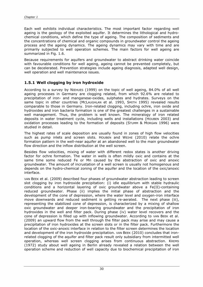
Chapter 1
30
Each well exhibits individual characteristics. The most important factor regarding well ageing is the geology of the exploited aquifer. It determines the lithological and hydro-chemical conditions, which define the type of ageing. The composition of sediments and the concentrations of chemical and organic compounds in groundwater control the ageing process and the ageing dynamics. The ageing dynamics may vary with time and are primarily subjected to well operation schemes. The main factors for well ageing are summarized in Fig. 1.6.
Because requirements for aquifers and groundwater to abstract drinking water coincide with favourable conditions for well ageing, ageing cannot be prevented completely, but can be decelerated. Prevention strategies include ageing diagnosis, adapted well design, well operation and well maintenance issues.
Well clogging by iron hydroxide 1.5.1
According to a survey by NIEHUES (1999) on the topic of well ageing, 84.0% of all well ageing processes in Germany are clogging related, from which 92.6% are related to precipitation of iron- and manganese-oxides, sulphates and hydrates. Surveys on the same topic in other countries (MCLAUGHLAN et al. 1993, SMITH 1995) revealed results comparable to those in Germany. Iron-related clogging, including ochre, iron oxide and hydroxides and iron bacteria formation is one of the greatest challenges in a sustainable well management. Thus, the problem is well known. The mineralogy of iron related deposits in water treatment cycle, including wells and installations (HOUBEN 2003) and oxidation processes leading to the formation of deposits (STUMM & MORGAN 1996) were studied in detail.
The highest rates of scale deposition are usually found in zones of high flow velocities such as pump inlets and screen slots. HOUBEN and WEIHE (2010) relate the ochre formation pattern in the well-near aquifer at an abandoned well to the main groundwater flow direction and the inflow distribution at the well screen.
Besides flow velocities, mixing of water with different redox states is another driving factor for ochre formation. The water in wells is often mildly oxic and contains at the same time some reduced Fe or Mn caused by the abstraction of oxic and anoxic groundwater. The amount of incrustation of a well screen is usually not homogenous and depends on the hydro-chemical zoning of the aquifer and the location of the oxic/anoxic interface.
VAN BEEK et al. (2009) described four phases of groundwater abstraction leading to screen slot clogging by iron hydroxide precipitation: (i) idle equilibrium with stable hydraulic conditions and a horizontal layering of oxic groundwater above a Fe(II)-containing reduced groundwater. Phase (ii) implies the initial phase of abstraction and the development of the cone of depression, where the water level and oxygen-iron interface move downwards and reduced sediment is getting re-aerated. The next phase (iii), representing the stabilized cone of depression, is characterized by a mixing of shallow oxic groundwater and deeper iron-bearing groundwater and the precipitation of iron hydroxides in the well and filter pack. During phase (iv) water level recovers and the cone of depression is filled up with inflowing groundwater. According to VAN BEEK et al. (2009) an upward flow from the well through the filter pack may arise and may cause a precipitation of iron hydroxides at the screen slots or in the filter pack. Furthermore the location of the oxic-anoxic interface in relation to the filter screen determines the location and development of the iron hydroxide precipitation. VAN BEEK (2010) concludes that iron-related clogging of the aquifer and filter pack result only subsidiary from intermitted well operation, whereas well screen clogging arises from continuous abstraction. KREMS (1972) study about well ageing in Berlin already revealed a relation between the well operation scheme and reduction of well capacity due to biochemical precipitation of iron

General introduction
31
hydroxides. Besides KREMS (1972), MOSER (1979) and TYRREL and HOWSAM (1990) observed a restoring effect of continuous abstraction for well capacity at an early stage.
After VAN BEEK (2010) three processes of iron oxidation and precipitation can be distinguished. These are (i) homogeneous oxidation of iron(II) by dissolved oxygen and immediate precipitation of iron(III) hydroxides, (ii) heterogeneous oxidation of iron(II) by adsorption and simultaneous or separated oxidation to an iron(III) surface complex and (iii) biological oxidation of iron(II) by iron oxidizing bacteria.
A coexistence of Fe(II) and DO in groundwater leads to a homogenous oxidation and precipitation of Fe(III) hydroxides (STUMM & MORGAN 1996).
In a first reaction Fe(II) is oxidized to Fe(III):
4 Fe2++ O2 + 4 H+ → 4 Fe3+ + 2 H2O (1)
In s second reaction Fe(III) is hydrolyzed to Fe(III)-hydroxide:
4Fe3++4 H2O→4Fe�OH�3↓ +4H+ (2)
The kinetics of Fe(II) oxidation has been topic of numerous studies. The reaction rate has a linear dependency on the Fe activity and on the partial pressure of DO, and a quadratic dependency on the hydroxyl activity. The half-life for the homogenous oxidation can be calculated as (STUMM & MORGAN 1996):
t12� =
ln2
k1 [H+]
2
[O2] (3)
In presence of Fe(III) hydroxides, oxidation of Fe(II) is catalysed due to an adsorption and hydrolysis of Fe(II) at mineral surfaces. This heterogeneous oxidation plays a significant role in ochre formation. As soon as Fe(III) hydroxides are present, e.g. in a well, the reaction rate increases and well clogging is promoted.
For more details of oxidation kinetics it is referred to STUMM and MORGAN (1996) and HOUBEN (2004).
The hydro-chemical process of Fe(II) oxidation is strongly mediated by specialised microorganisms such as Gallionella or Lepthothrix (Ivarson & Sojak 1978, Hanert 1981). They are common members of bacterial community of groundwater environments. The microorganisms are able to catalyse the oxidation processes and gain the energy for their metabolism (HALLBERG & FERRIS 2004). The iron oxidizing bacteria like Gallionella, Lepthothrix and Siderocapsa are able to adsorb iron to their cell material or/and to the exopolymers to enhance the iron(II) oxidation capacity (CULLIMORE & MCCANN 1978). Usually, iron oxidizing bacteria need conditions where oxygen and iron(II) are present, because oxidation of iron(II) gains only little energy and therefore the precipitation rate has to be high. Wells provide them with an excellent breeding ground since they are sedentary organisms and thus dependent on their nutrients to flow past them. If flow velocity exceeds natural flow conditions Fe(II)-concentrations of 0.2 mg/l and higher are sufficient for an extensive bacteria growth (CULLIMORE & MCCANN 1978). The biological oxidation of Fe(II) requires also slightly positive redox potentials at low or neutral pH (HÄSSELBARTH & LÜDEMANN 1967).
As long as flow velocities are in the range of natural flow gradients in groundwater a massive growth of iron-oxidizing bacteria is precluded (KREMS 1972). Only when flow velocities are significantly accelerated, as they are close to production wells, bacteria and biofilms might develop vastly. At the well screen area, where velocities are highest,

Chapter 1
32
biological oxidation of Fe(II) could even exceed the chemical oxidation rate of Fe(II) (SOBOLEV & RODEN 2002, WEBER et al. 2006). This effect is increasing with decreasing pH, because chemical oxidation is then reduced. EMERSON et al. (2010) summarized from several case studies, that the biological oxidation accounts for nearly 50% of the total oxidation rate. DRUSCHEL et al. (2008) actually identified in their study a biological oxidation ratio of 60 %. In addition to high biological oxidation rates, involved in ochre formation, biological oxidation is observed to already takes place in the well-near aquifer as long as flow velocities and nutrient supply are sufficiently high (TUHELA L et al. 1997).
Impact of well ageing on well management issues 1.5.2
Aim of an integrated well management is an optimum well operation in terms of water quality and water quantity. However, cost-efficiency plays a dominant role for well operators, too. An optimum well operation can only be obtained, when all elements affecting the well operation are integrated in a well management concept. This concept should include an adapted well design and construction based on the given hydrogeological setting, a well monitoring program feasible to identify well ageing processes and an appropriate well maintenance strategy to restore well performance and prolong well life time. For further information it is referred to WICKLEIN and STEUßLOFF (2006).
The state of the art concerning all elements of an integrated well management are well described in several publications. For detailed information about well management issues it can be referred to the most important documents (HOWSAM et al. 1995, MCLAUGHLAN 2002, HOUBEN & TRESKATIS 2007). Below, well management issues are only comprehensively summarized.
Well design and construction determine the flow velocity and inflow distribution and therefore influence the location of ageing deposits. The configurations, dimensions and choice of materials for well construction are set by a variety of economic, technical, quantitative and qualitative requirements. The hydraulic and technical design need to be evaluated for each new well site individually.
Well operation needs to fulfil requirements from demand, technical possibilities and economic efficiency. Any change in operation, which might prevent a certain process from occurring, might on the other hand enhance another. Basis to develop an operational schedule must be the evaluation of the ageing potential, including the dominant ageing type and the occurring processes (e.g. mixing, turbulent flow) to determine how they can be prevented.
Diagnosis of well ageing type and rate is a prerequisite for scheduling well operation and maintenance strategies. The identification of the ageing type requires information about the specific site conditions concerning geology, hydrochemistry and well construction.
To provide information on the development of performance and condition of a well, the well has to be monitored in constant intervals and generated data have to be processed and analysed.
According to HOWSAM et al. (1995) the following key parameter have to be determined for diagnosis:
• Condition of the well installations: Pump, rising main, casing, screen
• Condition of the filter pack (compared to a previous state): Pore space, permeability, active sections of intake
• Hydro-chemical site characteristics, which represent (i) the redox-conditions, (ii) mineral stabilities and (iii) the living conditions for microorganisms: O2, NO3-N, pH, Eh, Fe, Mn, Ca, HCO3, DOC, AOC, T

General introduction
33
• Water level: variability of static water level, drawdown, entrance resistance ∆h
• Well yield: Q-s-curve (compared to a previous state), Qs-development with time in operation, calculation of aquifer and well loss
Basically the assessment of well performance is done by the comparison of the actual ratio of the pumping rate Q and the respective drawdown s with the initial state of performance after well construction. If applied in constant intervals measurements of the Q/s-ratio illustrate the temporal development of well yield Qs, or respectively the well ageing rate. Well maintenance is an important component in well management, either to decelerate ageing processes or to rehabilitate well performance after deterioration occurred. A variety of measures is available and described by specialist books (HOWSAM et al. 1995, HOUBEN & TRESKATIS 2007). Preventive treatments like well disinfection should prevent the extensive growth of bacteria populations. The prophylactic treatment of ochre-endangered water wells with hydrogen peroxide solution for example should prevent transformation of iron related ochre and prevent hardening of existing minerals (Wicklein & Steußloff 2006). Basis for successful and sustainable well rehabilitation is a reliable monitoring and documentation of well performance data, the optimum point of time (e.g. 20% performance loss, referred to DVGW (2007) and the complete removal of detached deposits, which may serve as source for an early resettlement by ochre (SCHWARZMÜLLER et al. 2012).
Outline of the thesis 1.6
Chapter 1 already summarizes the motivation and topic of this thesis.
Chapter 2 characterizes Berlin’s drinking water wells concerning their design, operation, geological setting, hydro-chemical composition and maintenance activities. Results illustrate the vulnerability of wells for clogging processes and reveal the relevance of detailed investigations on this topic.
Chapter 3 gives a general estimation of the influence of the two main oxygen delivering processes, air entrapment and bank filtration, on groundwater aeration related to water abstraction by wells. A generic transport model simulates oxygen fluxes with regard to different hydrogeological and operational boundary conditions.
Chapter 4 quantifies the potential amount of oxygen which can be delivered to groundwater by fluctuating water levels under laboratory conditions. Column experiments with defined boundary conditions provide reference data comparable to modelling and field site results.
Chapter 5 investigates both oxygen delivery processes, air entrapment and bank filtration, at selected well sites in Berlin by in situ monitoring of oxygen in wells and aquifers. Results relate different geological settings and different well operation schemes to changes in oxygen fluxes and evaluate their effects on well ageing processes.
Chapter 6 describes the oxygen dependency of ochre formation with regard to well operation at a model well. The tank experiments enable to study distribution pattern of ochre formation with regard to the different structural zones of the well including aquifer, filter pack and screen slots and their influence on pressure losses and well performance.
Chapter 7 discusses the preventive treatment of wells with hydrogen peroxide by reviewing the latest research activities and by analysing and presenting laboratory and field site investigations. The current treatment procedure is evaluated with regard to an undesired oxygen release from dissociation processes, and an optimized application strategy concerning solution concentrations, treatment intervals and procedure is demonstrated.

Chapter 1
34
Chapter 8 presents a statistical approach to quantify well ageing and to identify factors promoting well performance loss. Most appropriate clogging indicators are identified and used to analyse worst and best site conditions with regard to ageing vulnerability.
Chapter 9 summarizes the essential outcomes and link the different investigations of each chapter to give recommendations for an optimized well monitoring and operation and to look ahead at open challenges in well management.

Characterization of Berlin well sites with regard to ochre formation
35
Chapter 2
Characterization of Berlin well sites
with regard to ochre formation
Introduction 2.1
Factors influencing the ochre formation at drinking water wells are already well known. However, interaction of factors and processes and its impact on well performance development is often ambiguous. The question arises how to detect well ochre formation at an early stage to impede well ageing.
One approach is to detect and characterise general well ageing pattern by statistical and descriptive analysis of existent well data sets. Therefore, the most important parameters influencing chemical and biological clogging processes e.g. geological and hydrogeological conditions, well design, well operation, well hydraulics, well maintenance, hydrochemistry and well performance need to be considered.
Geological boundary conditions, for example, strongly influence the flow field and hydrochemistry in the aquifer. Oxygen delivery by air entrapment and dissolution as consequence of water level fluctuations is one of the main challenges at preventing iron-related well clogging. The amplitude of water level oscillation and the shape of the depression cone, and therefore the amount of delivered oxygen, are primarily controlled by the permeability and the storage coefficient of the aquifer. The advective transport of oxidized groundwater and the flow velocity towards the well are other factors and subject to the aquifer characteristics, too.
Well design and location may also be a key parameter controlling ageing potential. The type and depth of filter screens, for instance. The depth of the (first) screen top can drastically affect the mixture of abstracted water, considering a supply of wells either by shallow oxic or by deep anoxic groundwater, by bank filtrate or by artificial recharged water. Shares of different water sources are also strongly connected to the distance of wells to surface water bodies as the distance influences travel times of bank filtrate, which again controls its redox status (FRITZ 2002, GRESKOWIAK et al. 2005).
Well operation may influence ochre formation, too. Since the effect of oxygen delivery by oscillating water levels becomes suspect in promoting ochre formation, well switchings are expected to enhance well ageing. Thus, the Berlin waterworks already established a classification of wells into wells with high ageing potential and wells with low ageing potential prior to the studies presented in this thesis. Those wells vulnerable to ochre formation, typically old wells, are switched as seldom as possible, whereas wells less vulnerable to ochre formation, typically new wells, switched more often. According to WICKLEIN and STEUßLOFF (2006), these operation schemes are described as permanently operated wells and short-term operated wells.
As hydro-chemical compounds in groundwater control the oxidation processes, their occurrence in abstracted well water may represent the ageing vulnerability of wells. It can be assumed, too, that hydro-chemical conditions may vary between different waterwork sites and therefore also their ageing potential of wells.
Thus, basing on a data base, including master and operational data of all Berlin drinking water wells, wells sites should be characterized for (i) the identification of clogging

Chapter 2
36
factors which may play a major role for ochre formation at Berlin wells and (ii) the identification of the scope for optimization of well design, well operation, well monitoring and well maintenance. Additionally, the analysis shall support the selection of test sites for a detailed investigation of oxygen delivery processes and their impact on ochre formation with regard to transferability of findings to other well sites.
Data analysis further has to proof validity of data sets and their applicability for the above mentioned tasks. Especially data quality of redox sensitive parameter and therefore significance of data is often limited by type and date of sampling.
Methods and materials 2.2
For the characterisation of well sites with focus on well ageing the local water utility Berliner Wasserbetriebe provides a data base including the most relevant information concerning well design, well operation, well maintenance and water quality. The analysed data set includes vertical wells, which were used for drinking water production during the years 1996 to 2008. This applies to 687 wells, but not all included wells provide the complete parameter set. The classification of aquifer types derived from hydrogeological cross sections of the single well fields also provided by the water utility.
Following parameter were considered for the well site characterisation:
1. Well age
2. Aquifer type
3. Well design parameter:
- Total well depth
- Depth to top of filter screen
- Total length of filter screen
4. Well operation parameter:
- Mean discharge rate
- Mean monthly operational hours
- Frequency of well switchings per month
5. Rehabilitation intervals
6. Hydro-chemical parameter:
- Main ions
- In situ parameter: O2, redox potential, pH, EC, DOC, Mn, Fe, NO3, NO2, NH4
All of the 687 vertical wells are arranged in well fields. Each well field consists of 5 to 59 wells and belongs to one of the 9 water works owned by the utility. Most wells are operated by the water work Friedrichshagen with 173 wells in 5 different well fields, the smallest water work is Kladow with only one well field and 14 wells (see also Tab. 2.1).

Characterization of Berlin well sites with regard to ochre formation
37
Tab. 2.1: Number of waterworks, well fields and vertical wells operated by the Berliner Wasserbetriebe (effective 2008)
Waterworks number of well fields number of wells
Beelitzhof 6 86
Friedrichshagen 5 173
Kaulsdorf 2 16
Kladow 1 14
Spandau 3 44
Stolpe 4 89
Tegel 7 120
Tiefwerder 4 55
Wuhlheide 2 89
Σ = 9 Σ = 34 Σ =687
Results 2.3
Well age 2.3.1
The Berlin water utility operates 687 wells, which currently (2008) have an age between 2 and 55 years (Fig. 2.1) and a mean well age of 23.3 years. The chronology of well construction revealed that construction activities are variable over time. In some years (while German reunion) a quantity of more than 50 wells were constructed whereas in other years (after reunion) construction was suspended. Obviously, political, operational and economic reasons influence well management and thus the data variability. Since recent wells were constructed throughout a time span of 55 years, their technical standard is not consistent concerning casing material, screen type, filter pack dimensioning, sealing philosophy and others.
Fig. 2.1: Histogram of well ages.
0 5 10 15 20 25 30 35 40 45 50 55Age of well [years]
0
20
40
60
80
Fre
qu
en
cy
n=687mean=23.3

Chapter 2
38
Aquifer type 2.3.2
Hence, differentiation of wells concerning their vulnerability to oxygen delivery by oscillating water tables can be done by simply classifying the hosting aquifers in hydraulically confined or unconfined aquifers. Confined aquifers are separated from atmospheric influence by aquitards, unconfined are not.
The number of drinking water wells in Berlin situated in uncovered aquifers (329) nearly equals the number of wells in covered aquifers (356). The highest ratio of covered wells is associated with the water work Kladow with 93% and Beelitzhof with 90%, whereas the lowest ratio of covered wells is referred to the water work Wuhlheide with only 22%. At other water works the ratio between wells in covered or uncovered aquifers is more balanced (see Fig. 2.2).
However, information from bore logs and their interpretation in hydrogeological cross sections can be delusive due to the heterogeneous and discontinuing distribution of interglacial sediments in the area of Berlin. To clearly identify, if wells really act as hydraulically unconfined or confined unit, data should best be verified by analysis of pumping tests and hydrogeological simulations in future studies.
Fig. 2.2: Number and ratio of wells in covered and uncovered aquifers.
Well design and location 2.3.3
The hydrogeological conditions of the Berlin well sites set the framework for well design and construction criteria. Total length and depth of wells, depth of screen top and distance to next surface water are more or less predefined by hydrogeology. For box plots of these parameters see Fig. 2.3.
Statistical analysis revealed that wells have depths between 15 and 170 m below ground with a mean depth of 40 m. But 50 % of the wells have a depth of around 40 m. This clarifies that depending on the waterworks site wells are mainly screened in the second and third aquifer complex.
Well screens have total lengths between 3 and 53 m, partly distributed to as many as 5 screened well sections. Mean screen length is about 14 m. Recently, Berlin wells are only screened in a single aquifer complex to prevent mixing and hydraulic interactions between the different aquifer complexes. Redundant screen sections, particularly at old wells, were sealed subsequently.
Shares of deep anoxic and shallow oxic groundwater in the well can depend on the depth of filter screens. The depth of the (first) screen top lies between 9 to 63 m below ground

Characterization of Berlin well sites with regard to ochre formation
39
and 25 m below ground surface in average. Thus, wells have strongly varying shares of water with different redox states with certainty.
Also analysis of well location shows a great variability. For Berlin, distance of wells to the next surface water body varies between 0 and 2030 m. Average distance is about 350 m. But, it has to be considered, that wells, even though they are located in proximate distance to rivers or lakes, may be hydraulically not or only minor connected to infiltrating surface waters, particularly, if they are screened in the 3rd aquifer complex.
Since stainless steel is nowadays the preferred casing and screening material, all wells in Berlin constructed after 1995 are equipped with stainless steel wire-wound screens (184 out of 687, see also App. 1). The favoured bore diameter is 900 mm with a casing diameter of 400 mm. Generally, installed filter pack is twofold, with a finer outer and a coarser inner gravel. The filter pack is sealed by a clay suspension layer at his top to prevent percolating water through the filter pack.
Fig. 2.3: Constructional and positional characteristics of Berlin wells.
Well operation 2.3.4
The basis for an assessment of well performance is the monitoring of most important operational data. Analysis of most relevant operational data is presented in Fig. 2.4. The mean monthly operational hours are 288 (hours), which correspond to a temporal utilization degree of 39%. 90% of the wells have a temporal utilization degree between 14% (105 hrs) and 75% (560 hrs). It has be considered that accuracy and comparability of data is limited by the fact, that water works use different methods to measure the operational hours. In some cases operation hours are only measured indirectly, like e.g. by electricity consumption of pumps.
The measured discharge rates have to be interpreted carefully. In the data base, these data originate from manual readings of flowmeters installed at the well head and/or calculation from the potential capacity of installed pumps. Both methods are susceptible for inaccuracies. Wells built after 2004 are equipped with electromagnetic flowmeters and volume metering will be done by automatical reading and recording in the near future. The currently available data set reveals a mean discharge rate of 85 m3/h, whereas 90% of the wells abstract between 50 and 155 m3/h.
Data analysis shows that in general, wells are switched 0.6 times per month, but for 90% of the wells, mean well switchings per month range from 0.1 to 2.2. Switching data set only includes wells of the water works Beelitzhof, Kladow, Spandau, Stolpe, Tegel and
Tiefwerder and therefore considers only 316 of the 687 wells.

Chapter 2
40
Fig. 2.4: Box plots of operational data most relevant for well ageing processes (switching data limited to WW Beelitzhof, Kladow, Spandau, Stolpe, Tegel and Tiefwerder).
Rehabilitation intervals 2.3.5
Rehabilitation of Berlin wells is done exclusively by mechanical methods. The most used methods besides brushing base on impulse techniques, such as shock blasting with water or explosives. Commonly, one or a combination of both techniques is applied depending on the ageing status and ageing type of the well and considering the construction material. Rehabilitation intervals at Berlin drinking water wells correspond to a decrease in well yield and to practical experience gained from years of operation. Data analysis revealed a mean rehabilitation interval of six years, but intervals vary in general between one and 16 years (Fig. 2.5).
Rehabilitation success is typically documented by pumping tests, performed before and after rehabilitation. Static and dynamic water level are determined and used for the calculation of specific well yield at the given discharge rate. As rehabilitation measures take place only every six years (in average), values for the specific well yield are sparse. This complicates the diagnosis of well ageing and the prediction of well performance development as well as the determination of the optimal rehabilitation interval.
Fig. 2.5: Histogram of well rehabilitation intervals (some wells were rehabilitated more often than once).

Characterization of Berlin well sites with regard to ochre formation
41
Hydrochemistry in general 2.3.6
Main ions, plotted in a piper-diagram provide a compact description of basic hydro-chemical characteristics (Fig. 2.6). For Berlin, the plots show that waterworks with presumably high shares of bank filtrate (Beelitzhof, Friedrichshagen, Tiefwerder, Stolpe) show a significant higher variability in hydrochemistry than those waterworks abstracting native groundwater. This variability indicates a mixing of water with different origins, e.g. bank filtrate and native groundwater. Because of artificial aquifer recharge by ponds, the hydrochemistry of Tegel well sites is expected to vary in a greater extent, but the abstracted water is comparatively homogeneous compared to other bank filtration sites. Additional factors have to be relevant for the composition of water chemistry. Presumably, the spatial range of wells and well fields supplying a water work can be an important factor. Thus, to conclude that hydro-chemical heterogeneity of water samples from different wells in a well field correlates with the clogging potential is not stringent and further parameter have to be taken into account for an analysis of the well ageing risk.
Fig. 2.6: Piper diagram of the main ions in abstracted well water of the different water works.
Clogging of wells by incrustations of iron and manganese oxides and hydroxides requires a certain amount of these ions in groundwater abstracted by the wells. According to DVGW (1970) a minimum iron concentration of 0.2 mg/l was supposed to be the threshold value for iron-related well clogging. A more recent study state the ideal living conditions for iron oxidizing bacteria are between 1.0 and 25 mg/l Fe(II) (DRISCOLL 1986). With concentrations of 0.02 to 16 mg/l (2.0 mg/l in average) dissolved iron in abstracted water, nearly all Berlin wells fulfill the conditions for chemical and biological iron oxidation.
Dissolved Mn(II) is also subject to chemical and biological oxidation and thus can cause clogging of wells. However, iron ochre is more common than manganese ochre and
100 80 60 40 20 0
Ca
0
20
40
60
80
100
Na+K
0
20
40
60
80
100
Mg
0 20 40 60 80 100
Cl
100
80
60
40
20
0
SO
4
100
80
60
40
20
0
HC
O3+C
O3
Ca +
Mg
20
40
60
80
SO
4 +
Cl
80
60
40
20
Berlin water works
Beelitzhof
Friedrichshagen
Kaulsdorf
Spandau
Stolpe
Tegel
Tiefwerder
Wuhlheide
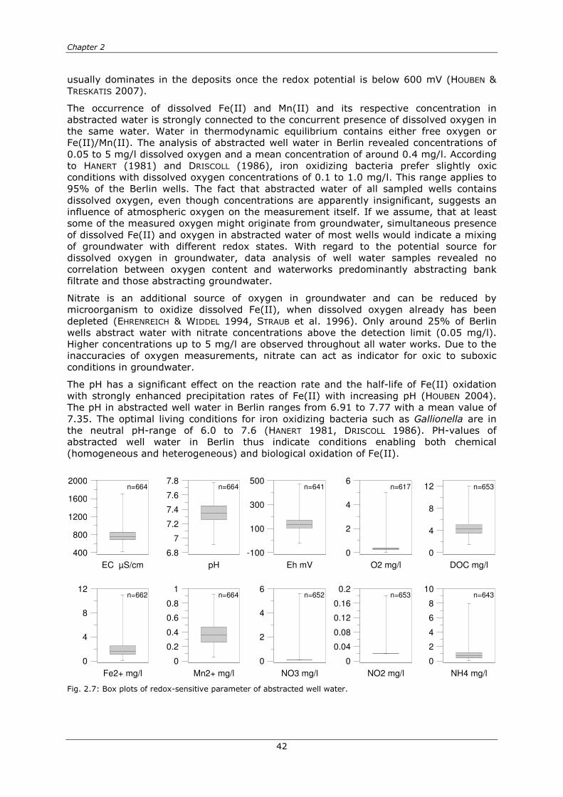
Chapter 2
42
usually dominates in the deposits once the redox potential is below 600 mV (HOUBEN & TRESKATIS 2007).
The occurrence of dissolved Fe(II) and Mn(II) and its respective concentration in abstracted water is strongly connected to the concurrent presence of dissolved oxygen in the same water. Water in thermodynamic equilibrium contains either free oxygen or Fe(II)/Mn(II). The analysis of abstracted well water in Berlin revealed concentrations of 0.05 to 5 mg/l dissolved oxygen and a mean concentration of around 0.4 mg/l. According to HANERT (1981) and DRISCOLL (1986), iron oxidizing bacteria prefer slightly oxic conditions with dissolved oxygen concentrations of 0.1 to 1.0 mg/l. This range applies to 95% of the Berlin wells. The fact that abstracted water of all sampled wells contains dissolved oxygen, even though concentrations are apparently insignificant, suggests an influence of atmospheric oxygen on the measurement itself. If we assume, that at least some of the measured oxygen might originate from groundwater, simultaneous presence of dissolved Fe(II) and oxygen in abstracted water of most wells would indicate a mixing of groundwater with different redox states. With regard to the potential source for dissolved oxygen in groundwater, data analysis of well water samples revealed no correlation between oxygen content and waterworks predominantly abstracting bank filtrate and those abstracting groundwater.
Nitrate is an additional source of oxygen in groundwater and can be reduced by microorganism to oxidize dissolved Fe(II), when dissolved oxygen already has been depleted (EHRENREICH & WIDDEL 1994, STRAUB et al. 1996). Only around 25% of Berlin wells abstract water with nitrate concentrations above the detection limit (0.05 mg/l). Higher concentrations up to 5 mg/l are observed throughout all water works. Due to the inaccuracies of oxygen measurements, nitrate can act as indicator for oxic to suboxic conditions in groundwater.
The pH has a significant effect on the reaction rate and the half-life of Fe(II) oxidation with strongly enhanced precipitation rates of Fe(II) with increasing pH (HOUBEN 2004). The pH in abstracted well water in Berlin ranges from 6.91 to 7.77 with a mean value of 7.35. The optimal living conditions for iron oxidizing bacteria such as Gallionella are in the neutral pH-range of 6.0 to 7.6 (HANERT 1981, DRISCOLL 1986). PH-values of abstracted well water in Berlin thus indicate conditions enabling both chemical (homogeneous and heterogeneous) and biological oxidation of Fe(II).
Fig. 2.7: Box plots of redox-sensitive parameter of abstracted well water.
0
4
8
12
DOC mg/l
n=653
400
800
1200
1600
2000
EC µS/cm
n=664
0
0.04
0.08
0.12
0.16
0.2
NO2 mg/l
n=653
0
2
4
6
8
10
NH4 mg/l
n=643
0
2
4
6
NO3 mg/l
n=652
0
0.2
0.4
0.6
0.8
1
Mn2+ mg/l
n=664
0
4
8
12
Fe2+ mg/l
n=662
-100
100
300
500
Eh mV
n=641
0
2
4
6
O2 mg/l
n=617
6.8
7
7.2
7.4
7.6
7.8
pH
n=664

Characterization of Berlin well sites with regard to ochre formation
43
To do a first assessment of the redox conditions in the aquifer and of the abstracted water, the redox potential Eh can be consulted. The redox potential of abstracted well water represents the mixing ratio of the different redox zones present in the aquifer and can be used to identify, if redox conditions, providing the oxidation of Fe(II), are existent. With redox potentials between -20 to 470 mV most abstracted waters are in the range of Fe (180-400 mV) and Mn (220-500 mV) reduction, whereas few waters suggest incipient reduction of nitrate (>300 mV) or sulphate (<100 mV). Hence, Berlin wells are not providing redox conditions suitable for chemical iron oxidation. But KREMS (1972) stated that iron-related well clogging already occurs at wells as soon as the redox potential is positive. This applies to almost all Berlin wells. According to HANERT (1981) and DRISCOLL (1986) iron oxidizing bacteria prefer redox potentials between 200 and 300 mV. Thus, most of Berlin wells do not reflect optimal conditions for biological oxidation of Fe(II). Values of redox potential have to be regarded suspiciously and comparability of values is only given, when the identic probe was used for measurement. The sampling accuracy can be assumed to ±50 mV.
Evaluation of redox sensitive parameter 2.4
Because already existent hydro-chemical data represent only a single point of time, with no regard to the phase of water abstraction, a time-dependent hydro-chemical monitoring of selected well sites should evaluate the representativity and reproducibility of existing hydro-chemical data. Furthermore, the newly developed monitoring program should assess the impact of short-termed variations in water chemistry on potential well ageing processes. The (short-term) monitoring is able to recognize variations in hydro-chemical parameters during the initial phase of pumping, which may potentially induce ochre formation in the well.
During the initial phase of water abstraction, a cone of depression develops in the water table. Parallel to the water table the interfaces of redox zones present in the aquifer move down. This causes a migration of oxygen-containing water into anoxic sediments (VAN BEEK 2010) and a mixing of oxygen-containing and iron-bearing groundwater as they both enter the well at the screen top. Therefore redox reactions might occur as soon as groundwater with different redox states mixes. This process is expected to be accompanied by varying hydro-chemical conditions. Finally, when flow field stabilizes and mixing occurs with a constant ratio, hydro-chemical conditions should be stable, too.
Methods 2.4.1
To provide comparability between the different wells, the following fixed sampling procedure was designed:
- shut-down of the well and its two neighbour wells for a minimum of one week before sampling
- start of the sampling equal to the time of switching on well
- sampling interval is every minute for the first ten minutes, then 15, 20, 30 min, and subsequently every half an hour
- sampling proceeds until stable physicochemical conditions are observed (variations within one hour): pH (±0.05), redox-potential (±10), O2 (=0), conductivity (±10), temperature (±0.5),
The first sample was taken directly after switching on the pump, to characterize the conditions in the well during shutdown; the second sample after one minute represents the initial pumping phase; the last sample represents the steady flow system with stable field parameters. Critical parameters like HS-, NH4, NO2
-, colour, turbidity and HCO3- were

Chapter 2
44
determined in situ. The drawdown within the well was measured with an electric contact meter at sampling intervals. Samples for analysis of main ions were filtered with cellulose acetate filters with a pore size of 0.45 µm. Cation samples were acidified with concentrated HNO3 to avoid precipitation of oxides or hydroxides. Besides the filtered cation sample, an unfiltered, acidified sample was taken for the investigation of particulate Fe(III) and Mn(IV) in the water.
Results 2.4.2
Summarizing the results of the short-term monitoring, almost all investigated wells showed high variations in several parameters directly after switching on the well. Especially the particulate and dissolved iron content, as well as the redox sensitive field parameters, seems to be significantly influenced by the change of the pumping regime. Abstracted water at all investigated wells (except for one) was free of detectable oxygen after maximum two hours of abstraction (Fig. 2.8). Although abstracted water is not in thermodynamic equilibrium and the well thus prone to precipitation processes, oxygen is not feasible as indicator for clogging processes due to its prevailing absence in well water.
From the short-term monitoring data and chemical analyses it becomes apparent, that
abstracted well water is not in a thermodynamic equilibrium (Fig. 2.9). Presence of oxygen (up to 10 mg/l) and nitrate (up to 14 mg/l) was proven under redox conditions where they should be absent in an equilibrium state. Fe(II) and Mn(II) are still present in zones, where they should be oxidized in equilibrium, but otherwise depleted in zones with low redox-potentials where higher contents can be expected. These conditions are for example affected by the mixing of reduced Fe(II)-bearing groundwater and oxygen-containing surface-near water and therefore provide chemical conditions for ochre formation.
For the future characterisation of well water, it should be taken into account that the stable physicochemical conditions are not reached until 90 to 120 min after start of abstraction, as revealed by the short-termed monitoring. It can be expected that beyond these short-termed variations, further hydro-chemical changes in greater timescales occur. These may be induced or at least influenced by varying operational schemes in a well field. Mid-term and seasonal changes were also investigated within the project WELLMA and partly presented by SCHWARZMÜLLER and MENZ (2013).
Fig. 2.8: Temporal variability of oxygen concentrations in well water related to the duration of water abstraction. For the temporal variability of redox potential see App. 2.

Characterization of Berlin well sites with regard to ochre formation
45
Fig. 2.9: Concentrations of O2, NO3, NH4 (above) and Fe(II) and Mn(II) (below) in the abstracted well water with regard to the respective redox potential. Solid lines represent the expected values for stable thermodynamic conditions.
Conclusions 2.5
The analysis of the characteristics of the Berlin drinking water abstraction wells with regard to ochre formation clearly point out their vulnerability to well ageing. Pre-conditions for ochre formation processes are fulfilled in most of the wells. Hence, the optimization of well design, operation and maintenance is promising benefit. This is already obvious considering the age distribution of Berlin wells. With a mean age of 23 years, but a maximum age of 55 years life-extending measures would be cost-effective.
Several factors were identified which are able to promote the ageing of Berlin wells by ochre formation. Half of the wells are situated in uncovered aquifers, which may favour iron oxidation processes by oxygen delivery due to water level oscillations. Most of the wells are only 40 m deep with screen length greater than 10 m beginning 20 m below ground. This means, travel times of potential oxic water from shallow groundwater to the screen top are comparatively short. The relevance of an oxygen delivery by bank filtrate is reflected by short distances of wells to surface water bodies.
0
2
4
6
8
10
12
14
-100 0 100 200 300 400
Redoxpotential [mV]
O2
& N
O3 [
mg
/l]
0
1
2
3
4
NH
4 [
mg
/l]
O2
NO3
NH4
0
1
2
3
4
5
-100 0 100 200 300 400
Redoxpotential [mV]
Fe
[m
g/l
]
0
0.2
0.4
0.6
0.8
1
Mn
[m
g/l]
Fe
Mn

Chapter 2
46
Also, hydro-chemical conditions identify the risk for ochre deposition in wells. Particularly, these are Fe(II) concentrations of around 2 mg/l and to a lesser extent Mn(II) with 0.3 mg/l, moderate pH-values around 7.4, redox potentials around 150 mV and traces of oxic species, like O2 and NO3.
Further, a newly developed sampling procedure, considering short-termed variations in redox sensitive parameters, demonstrated the temporal dependency and variability of hydrochemistry on the corresponding well operation state. Stable conditions are generally present after 90 to 120 minutes of water abstraction. Still, most wells are not in a thermodynamic equilibrium, since they contain reduced and oxidized species at redox potentials where they are incompatible at equilibrium.
Furthermore, analysis of operational well data revealed potential for the development of optimized well operation strategies. Both, a temporal utilization degree of 53% and a range in discharge rate from 50 to 155 m3/h, as well as switching frequencies, give room for improvements.

Simulation of oxygen transport towards a drinking water well
47
Chapter 3
Simulation of oxygen transport
towards a drinking water well
Introduction 3.1
The appearance of dissolved oxygen in iron-reducing aquifers is the decisive agent driving the iron-related well ageing. As known from bank filtration studies performed by MASSMANN et al. (2006b) at different well sites in the city of Berlin, surface water and bank filtrate provide dissolved oxygen under specific hydrogeological and climatic conditions. KOHFAHL et al. (2009) already calculated the significance of certain oxygen sources and paths towards a drinking water well in a site specific case. They identify air entrapment and bank filtrate as most important oxygen sources in groundwater at the investigated well site. Abstraction of groundwater and seasonal variations of surface water levels cause the most relevant oscillation amplitudes and therefore determine high input rates of dissolved oxygen in the aquifer. The oxygen amount in bank filtrate, given by KOHFAHL et al. (2009), varies between 0.2 mg/l in summer and 5 mg/l in winter.
The relevance of these two oxygen path-ways for oxidation processes close to and in the abstraction wells is not mentioned in literature so far. Indeed, influence of both oxygen sources on oxidation dynamics depends mainly on the hydrogeological setting, but the influence is also depending on the well design. To give a first approximation on the relevance of the two main oxygen sources in groundwater flow and transport of oxic water under pre-defined, for the Berlin site representative, conditions should be simulated. Therefore, flow and transport can be studied by simulating the mass transport towards a drinking water well in a generic geological environment with varying hydrogeological conditions.
Results of this modelling approach should clarify the impact of varying hydrogeological conditions on the mass transport towards an abstraction well with regard to iron-related well ageing. The model exercise should also provide an assessment of potential sources and risks for iron-related well ageing with regard to site-specific characteristics of the given location of a well site. The model should also provide the basis for a comparison with field data. In order to validate the simulation results, dissolved oxygen concentrations are measured in groundwater along observation transections at three different well sites in Berlin. In a future step a site specific simulation based on the generic model and the field site data is feasible.
A numerical, three-dimensional model should perform the requested task. The transport of dissolved oxygen is simulated in a transient solute transport model.
The degradation of oxygen during the infiltration of surface water and in the aquifer depends on various factors and processes and is complex when considered in detail. Hence, dissolved oxygen is here treated as inert compound and biological and chemical degradation along the flow path is not considered. Furthermore, the generic model does not include recharge and water level changes. Thus, seasonal variations or anthropogenic impacts are disregarded.

Chapter 3
48
Methods 3.2
Hydrogeological setting and conceptual model 3.2.1
The potential hydrogeological setting is derived from real well sites in Berlin.
Berlin wells are mostly situated in Quaternary aquifers made of glacial and fluvial, middle to coarse sediments. Aquifer thickness varies from 20 to 100 m and is often delimited by interbedded aquitards.
Wells used for drinking water production in Berlin are between 15 and 170 m deep with a mean depth of 40 m. But almost half of the wells have also a depth of around 40 m. These wells abstract water from the second aquifer complex. Further, a significant amount of wells have a depth of around 80 m. Those wells primarily penetrate the third aquifer complex. The depth of the top of the most upper screen section lies between 9 to 63 m below ground and 25 m below ground in average. Thus, well depth in the generic model is set to 40, respectively 80 meters.
Apart from the well depth, especially the location and the length of the filter screen affect the influx of, for example, deep groundwater or shallow bank-filtrate. Filter screen lengths vary between 3 and 53 m. Mean screen length of wells is about 14 m. However, most of the wells situated in the second aquifer complex feature screen length around 20 m, respectively around 40 m, when situated in the third aquifer complex. Therefore, the length of filter screen for the simulation is set to 20, respectively 40 meters.
Both, well depth and filter screen length are summarized and combined for two different scenarios. In a first scenario, representing water abstraction from aquifer complex 2, the filter screen is located in depth from 20 to 40 meters, in a second scenario, representing water abstraction from aquifer complex 3, from 40 to 80 meters below ground (see Fig. 3.1).
Fig. 3.1: Conceptual model: sources and pathways of oxygen in the aquifer induced by abstraction of groundwater and/or bank filtrate by a drinking water well (simplified scheme, e.g. depression cone).
The hydrogeological setting of the well site is important as well. Apart from the existence of surface water bodies, the heterogeneity of hydraulic conductivities, corresponding to an interbedding of coarse glacial and fine interglacial sediments plays a decisive role for

Simulation of oxygen transport towards a drinking water well
49
the composition of the abstracted water. Hydraulic conductivities vary around 10-4 m/s for the coarse grained aquifers. The fine grained interbedded units are less conductive with around 10-6 m/s, whereas the interglacial aquitards are only barely conductive with kf-values down to 10-9 m/s.
The discharge rate of the abstraction well has also a significant effect on the mixing ratio. Production wells in Berlin abstract from 10 to 150 m3/h, depending on the well site, the well age and the well design. In average, wells used for drinking water production in Berlin abstract around 80 m3/h.
The influence of these different boundary conditions causes different concentrations of oxygen in the abstracted well water as well as in the well near aquifer.
Potential sources of dissolved oxygen are, as mentioned above, bank filtrate and oxidized groundwater due to air entrapment. This modelling approach does not consider the process of air entrapment itself, but simulate the transport of the already oxidized groundwater from the cone of depression towards the well. The thickness of the oxic groundwater layer formed by water level fluctuations corresponds to the shape of the cone of depression for the respective discharge rate.
Dissolved oxygen concentration in the surface water and in the groundwater, filling the cone of depression, is set to 10 mg/l to simplify matter. As dissolved oxygen concentration of the surface water is fixed, concentrations of the resulting oxic groundwater layer vary between fixed and transient, depending on the approach. DO concentrations in groundwater may be overrated, because the approach assumes, that soil air is in equilibrium with atmosphere and degradation is excluded. This will result in a maximum input of DO into the aquifer and has to be considered in the conclusions.
The influence of surface water and therefore the rate of bank or artificially recharged filtrate on the abstracted groundwater are additionally influences by the colmation degree of the surface water body. The kf-value of the colmated layer was chosen to be 10-6 m/s. Thus, if colmation is considered in the simulation it reflects an early stage of the lake or river bed colmation. The conceptual model including the generic hydrogeological conditions and the well design is shown in Fig. 3.1.
Model design 3.2.2
The code used for the flow simulation is MODFLOW2000 and for the solute transport MT3DMS. Numerical approximation is done with the 3D finite differences method. The spatial dimension of the model was chosen according to the maximum extension of the depression cone. Grid spacing is varying, with decreasing nodal spacing (1.5 to 2 times) towards the abstraction well.
The flow is simulated in 3d. Based on the assumption of a radial flow towards the production well, the solute transport is simulated in a vertical cross section (Fig. 3.2).
Heads of the model boundaries in groundwater flow direction are constant. The model aquifer is unconfined with a natural flow gradient of 0.1 %. The lateral and vertical expansion of the cone of depression corresponds to a discharge of 80 m3/h, respectively 40 m3/h, depending on the scenario. The surface water body is represented by constant head cells in the three most upper layers, which corresponds to a maximum water depth of 5 meters. The lateral distance from the production well to the surface water body is about 100 meters.
The grid design, general boundary conditions and fixed parameters are presented in Tab. 3.1 and Fig. 3.2.

Chapter 3
50
Tab. 3.1: Model design and initial conditions.
Properties / Parameter Unit Shallow aquifer Deep aquifer
Layers - 12 13
Rows - 60
Columns - 118
Dimensions x 1000
y 1000
z 40 80
Nodal grid spacing - factor - 1-2
Simulation time Days 1000
Vertical hydraulic conductivity m/s 1.00E-05
Horizontal hydraulic conductivity m/s 1.00E-04
Hydraulic conductivity of colmated layer m/s 1.00E-06
Initial concentration dissolved oxygen mg 10
Specific storage - 1.00E-05
Specific yield - 2.50E-01
Effective porosity - 0.25
Dispersion longitudinal - 1.00E-01
Dispersion transversal - 1.00E-02
Dispersion vertical - 1.00E-02
Top of filter screen m b. s. 20 40
Bottom of filter screen m b. s. 40 80
Fig. 3.2: Model grid and boundary conditions in vertical cross section used for solute transport modeling.

Simulation of oxygen transport towards a drinking water well
51
Scenarios 3.2.3
Impact of different hydrogeological conditions on the oxygen delivery 3.2.3.1
This approach examines the impact of different hydrogeological boundary conditions on the DO distribution in the aquifer. 22 scenarios where chosen to display the influence of varying:
- oxygen sources (groundwater/ bank filtrate)
- aquifer thicknesses ( 40m / 80m)
- colmation degrees of the bank (permeable/ colmated)
- aquifer type (unconfined/ semiconfined/ confined)
- discharge rates (40/ 80 m3/h)
All scenarios imply a constant input of DO, whether the source is shallow groundwater or bank filtrate. A constant DO concentration in shallow groundwater requires frequent water table oscillations entrapping and solving the oxygen, which is supplied by the atmosphere and transported through the soil. Tab. 3.2 lists the different model scenarios. The aquifer type is represented by varying hydraulic conductivities in layer 4 and 5. In the unconfined case kf-value is assigned to be 10-4 m/s. In the semiconfined and the confined case kf-value is set to 10-6 and 10-8 m/s, respectively.
Tab. 3.2: Boundary conditions of different model scenarios. (GW=groundwater, BF=bank filtrate; perm.=permeable, colm.=colmated; hydraulic conductivities only varying for layer 4 and 5)
Scenario
Oxygen
source
Aquifer
thickness Bank
type
Kfh/Kfv Kfhorizontal Kfcolmation Discharge
rate
[GW,BF] [m] - [m/s] [m/s] [m3/h]
1 GW 40 Perm. 0.1 1.00E-04 - 80
2 GW 40 Perm. 0.1 1.00E-06 - 80
3 GW 40 Perm. 0.1 1.00E-08 - 80
4 GW 80 Perm. 0.1 1.00E-04 - 80
5 GW, BF 40 Perm. 0.1 1.00E-04 - 80
6 GW, BF 40 Colm. 0.1 1.00E-04 1.00E-06 80
7 GW, BF 40 Perm. 0.1 1.00E-06 - 80
8 GW, BF 40 Perm. 0.1 1.00E-08 - 80
9 GW, BF 80 Perm. 0.1 1.00E-04 - 80
10 GW, BF 80 Colm. 0.1 1.00E-04 1.00E-06 80
11 GW, BF 80 Perm. 0.1 1.00E-06 - 80
12 BF 40 Perm. 0.1 1.00E-04 - 80
13 BF 40 Colm. 0.1 1.00E-04 1.00E-06 80
14 GW 40 Perm. 0.1 1.00E-04 - 40
15 GW 40 Perm. 0.1 1.00E-06 - 40
16 GW 80 Perm. 0.1 1.00E-04 - 40
17 GW, BF 40 Perm. 0.1 1.00E-04 - 40
18 GW, BF 40 Colm. 0.1 1.00E-04 1.00E-06 40
19 GW, BF 40 Perm. 0.1 1.00E-06 - 40
20 GW, BF 80 Perm. 0.1 1.00E-04 - 40
21 BF 40 Perm. 0.1 1.00E-04 - 40
22 BF 40 Colm. 0.1 1.00E-04 1.00E-06 40

Chapter 3
52
Impact of source type on oxygen concentrations in the well 3.2.3.2
Scenarios D1 and D2 consider a transient delivery and input of DO towards the shallow groundwater. They only vary in the given discharge rate. The transient delivery and input of DO is here representative for a single water table oscillation event, for example a single well switching, resulting in the relocation of already oxic shallow groundwater into greater depth with the ongoing drawdown of the depression cone. The amount of shallow oxic groundwater is therefore limited and corresponds to the volume of the depression cone. A scenario overview is given by Tab. 3.3.
Tab. 3.3: Specific boundary conditions for different scenarios
Scenario Aquifer type Bank type Discharge rate [m3/h] Source of solute
D1 Unconfined Shallow Permeable 80 Transient
D2 Unconfined Shallow Permeable 40 Transient
Results 3.3
Impact of different hydrogeological conditions on the oxygen 3.3.1
delivery
The simulation results, shown in Fig. 3.3 for high discharge rates (80 m3/h) and in Fig. 3.4 for low discharge rates (40 m3/h), indicate highest input concentrations of DO in case of an unconfined shallow aquifer and high discharge rates (S1 and S5). The combined input of DO by infiltrating surface water and water level oscillations is slightly higher than solely by water oscillations.
Concerning high discharge rates, lowest DO concentrations are simulated for aquifers with confined conditions (S3 and S8). Within the observed time scale DO does not enter the aquifer below the confining layer, whether the source is oxic groundwater or infiltrating surface water.
As expected, travel times of oxic groundwater and bank filtrate in semiconfined aquifers (S2 and S7) are prolonged compared to those in unconfined ones. Highest DO concentrations are simulated for semiconfined conditions with combined input of oxic bank filtrate and groundwater. However, high DO concentrations are limited here to the upper, well permeable layer.
Regarding the simulated results for deep aquifers, DO enters the unconfined aquifer delayed in time and is also limited to the upper aquifer layer (S9 and S10). In case of semi-/confined deep aquifers (S11) travel times of oxic groundwater and bank filtrate distinctly exceed the simulation time, thus these scenarios are not further considered.
If infiltrating surface water is assumed to be the only source of DO in the shallow aquifer system (S12), concentrations first rise in the deeper section of the aquifer corresponding to the filter screen of the well. Then DO concentrations in the upper aquifer start to increase, followed by an increase in the bank filtrate averted direction. Total concentrations remain in this case markedly below those, which were observed in S1 and S5.
By comparing simulation results of scenarios with high discharge rates (80m3/h) and scenarios with low discharge rates (40m3/h) deviations are obvious. In nearly all low discharge scenarios (S14-S22) the first appearance of DO is postponed noticeably, followed by a protracted rise. Except for cases in which the well abstracts water from a deep aquifer (S16 and S20). Independent of the source of DO, abstraction does not result in a rise of concentrations in the aquifer within the simulated time of 1000 days.

Simulation of oxygen transport towards a drinking water well
53
Regarding scenarios 17 and 18, a colmation of the surface water bank and therefore lower infiltration rates induce lower DO concentrations in all observation points compared to unclogged conditions. The simulation results show elevated concentrations in the bank filtrate directed observations. This can be explained by a stronger influence of the natural flow gradient on the DO distribution and therefore a higher discharge of groundwater.
When considering infiltrating surface water as only source of DO, it is also obvious that concentrations first arise in the depth related to the well screen followed by an appearance in upper aquifer layers. Additionally a colmation of the bank only slightly affects the input of DO. Compared to DO distribution induced by high discharge rates the up gradient groundwater is free of DO at a low discharge rate.
The natural flow gradient generally affects the DO distribution to a higher extent when discharge rates are low. This is documented by an increase of the concentrations down gradient.
Tab. 3.4 gives the minimal travel times of the solute to the well for the different boundary conditions (scenarios). The calculated minimal travel time (or maximum effective flow velocity) to the well for the different scenarios varies from 90 to >1000 days. Shortest travel times (90 days) are estimated for high discharge rates and unconfined conditions. Lower pumping rates and also leaky conditions induce a distinct extension of travel times. It is also apparent, that in this approach DO from infiltrating surface water takes thrice the time to well than DO from groundwater surface. Long travel times are associated with leaky and confined shallow aquifers as well as deep aquifers regardless if phreatic, leaky or confined.
Tab. 3.4: Calculated travel times of oxic groundwater or/and bank filtrate towards the abstraction well.
Oxygen
source Hydraulic
condition
Aquifer
thickness Bank type
Minimal travel time of solute to the
well [days]
[GW,BF] [m] 80 m3/h 40 m3/h
GW Unconf. 40 Perm. 90 320
GW Semiconf. 40 Perm. 420 >1000
GW Conf. 40 Perm. >1000 -
GW Unconf. 80 Perm. >830 >1000
GW, BF Unconf. 40 Perm. 90 310
GW, BF Unconf. 40 Colm. 90 310
GW, BF Semiconf. 40 Perm. 390 >1000
GW, BF Conf. 40 Perm. >1000 -
GW, BF Unconf. 80 Perm. >1000 >1000
GW, BF Unconf. 80 Colm. >1000 -
GW, BF Semiconf. 80 Perm. >1000 -
BF Unconf. 40 Perm. 310 770
BF Unconf. 40 Colm. 420 >1000

Chapter 3
54
Fig. 3.3: Graphical presentation of the results of the solute transport simulation. Discharge rate is 80 m3/h. Observation points are situated in 3m distance from the well axis and oriented bidirectional parallel to the flow direction. Oxygen originate from groundwater (GW), bank filtrate (BF) or both (GW/BF).
0
2
4
6
8
cO
2 [
mg
/L]
S1GW - unconfinedshallow aquifer
S2GW - semiconfined
shallow aquifer
S3GW - confinedshallow aquifer
0
2
4
6
8
cO
2 [
mg
/L]
S4GW - unconfined
deep aquifer
S5GW/BF - unconfined
shallow aquifer
S6GW/BF - unconfined
colmated bankshallow aquifer
0
2
4
6
8
cO
2 [
mg
/L]
S7GW/BF - semiconfined
shallow aquifer
S8GW/BF - confined
shallow aquifer
S9GW/BF - unconfined
deep aquifer
0
2
4
6
8
cO
2 [
mg
/L]
S10GW/BF - unconfined
colmated bankdeep aquifer
0 200 400 600 800 1000Time [days]
S11GW/BF - semiconfined
deep aquifer
0 200 400 600 800 1000Time [days]
S12BF - unconfinedshallow aquifer
0 200 400 600 800 1000Time [days]
0
2
4
6
8
cO
2 [m
g/L
]
Observation depth (meter below static water level)GW - 7 m
GW - 13 m
GW - 20 m
GW - 30 m
BF - 7 m
BF - 13 m
BF - 20 m
BF - 30 m
S13BF - unconfinedcolmated bankshallow aquifer

Simulation of oxygen transport towards a drinking water well
55
Fig. 3.4: Graphical presentation of the results of the solute transport simulation. Discharge rate is 40 m3/h. Observation points are situated in 3m distance from the well axis and oriented bidirectional parallel to the flow direction. Oxygen originate from groundwater (GW), bank filtrate (BF) or both (GW/BF).
Fig. 3.5 shows the occurrence and the development of DO concentrations in abstracted well water. The range of absolute concentrations is between 0 and 1.5 mg/l. The maximum concentrations are related to an abstraction of oxic groundwater at high discharge rates. A combined input of oxic groundwater and infiltrating surface water results in maximum concentrations of 1.2 mg/l. In case of a clogged bank, concentrations degrade to a maximum of around 1.0 mg/l. Leaky conditions cause a maximum input of 0.8 mg/l. Insignificantly lower concentration around 0.7 mg/l are simulated, when input of DO is limited to infiltrating surface water. A further significant reduction of DO in well water to a maximum of 0.2 results from a colmation of the surface water bank.
0
2
4
6
8
cO
2 [m
g/L
]
S14GW - unconfinedshallow aquifer
S15GW - semiconfined
shallow aquifer
S16GW - unconfined
deep aquifer
0
2
4
6
8
cO
2 [m
g/L
]
S17GW/BF - unconfined
shallow aquifer
S18GW/BF - unconfined
colmated bankshallow aquifer
S19GW/BF - semiconfined
shallow aquifer
0 200 400 600 800 1000Time [days]
0
2
4
6
8
cO
2 [
mg
/L]
S20GW/BF - unconfined
deep aquifer
0 200 400 600 800 1000Time [days]
S21BF - unconfinedshallow aquifer
0 200 400 600 800 1000Time [days]
Observation depth (meter below static water level)
GW - 7 m
GW - 13 m
GW - 20 m
GW - 30 m
BF - 7 m
BF - 13 m
BF - 20 m
BF - 30 m
S22BF - unconfinedcolmated bankshallow aquifer

Chapter 3
56
A decrease of 50% in discharge rate strongly affects the DO concentrations in abstracted well water. It causes a distinct extension in travel time and a less increase of concentrations. But maximum concentrations are degraded marginally. This is only related to conditions, where DO originate from oxygenated groundwater. Travel times of bank filtrate exceed 800, respectively 1000 days when colmated, and concentrations are still transient at end of simulation.
According to the simulation, the highest potential input of DO into the well arises from oxygenated groundwater. As mentioned above, thickness of the initial oxic groundwater layer might be overestimated in reference to the specific discharge rate and therefore maximum concentrations are overvalued.
It is obvious that a 50% reduction of the discharge from 80 to 40 m3/h triplicate the travel times.
Fig. 3.5: Results of the solute transport simulation. Graphs show DO concentrations at the top of the filter screen of the production well as function of simulated time. DO concentrations >0 were observed for shallow aquifers only. Upper graph represents development of DO concentrations for a discharge rate of 80m3/h, lower graph for a discharge rate of 40m3/h.
0 200 400 600 800 1000Time [days]
0
0.2
0.4
0.6
0.8
1
1.2
1.4
1.6
1.8
2
cD
O [
mg
/L]
Discharge rate: 40m3/h
0 200 400 600 800 1000Time [days]
0
0.2
0.4
0.6
0.8
1
1.2
1.4
1.6
1.8
2
cD
O [
mg
/L]
GW/BF-unconf.
GW/BF-unconf.-colm.
GW/BF-semiconf.
GW-unconf.
GW-semiconf.
BF-unconf.
BF-unconf.-colm.
Discharge rate: 80m3/h

Simulation of oxygen transport towards a drinking water well
57
Impact of source type on oxygen concentrations in the well 3.3.2
Simulation results revealed that a transient DO source produce maximum DO concentrations at the top of the well screen which are 30% lower than under constant input conditions Fig. 3.6. Lower discharge rates can further reduce the maximum DO concentration occurring at the well screen. A reduction of the discharge rate by half, from 80 to 40 m3/h, under constant input conditions results in a decrease of maximum DO concentrations of 20%. Under transient input conditions this decrease is about 30%.
This effect, the quantitative stronger dilution of shallow oxic groundwater is only considered by the transient approach. A transient source of DO is also the more probable scenario, which displays only sporadically occurring well switchings.
Fig. 3.6: Development of simulated dissolved oxygen (DO) concentrations at the top of the filter screen as function of a constant source (representative for frequent switchings) and a transient source (representative for a single, nonrecurring switching) and the discharge rate of the well.
Conclusions 3.4
Aquifers with a reduced redox state and dissolved Fe contents provide high potential for depositing of precipitates when flow velocities and/or redox conditions change. Modification of flow gradients and velocities may result from anthropogenic action by aquifer management and water exploitation. Changes in redox conditions may occur by entry of DO into the aquifer. Abstraction of groundwater by wells cause a mixing of reduced, iron containing and oxic waters in the catchment area, preferred in the well near aquifer and the well itself.
Attention is directed to the input of DO by air entrapment caused by water level oscillations and infiltrating surface water. By neglecting degradation effects of the DO in the aquifer and during the infiltration the results has to be treated as worst case scenarios. The only DO sink in the model is abstraction by the well.
Results of the model simulation reveals oxygenated groundwater as the most important source of DO in the aquifer under the given boundary conditions and if degradation processes are excluded. Infiltrating surface water has a less but not minor potential as DO source. By reducing discharge rates or intense colmation of the surface water bank input of DO into the aquifer is or can be decreased significantly.
As expected, confined hydraulic conditions prevent the travel of DO enriched water into deeper aquifer zones and therefore protect the well against a mixing of oxic and anoxic, iron-containing water.
Leaky or semiconfined conditions impede shallow, oxic groundwater or/and bank filtrate to reach the subjacent aquifer and to get abstracted by the well.
0 200 400 600 800 1000Time [days]
0
0.5
1
1.5
cD
O [
mg/L
]
Discharge 80m3/hsingle osc.
constant osc.
Discharge 40 m3/hsingle osc.
constant osc.

Chapter 3
58
Wells with filter screens located in a great depth (in the model >40 m) with a thick overlying groundwater body are less endangered by oxic recharge. This is caused by high fraction of deep, anoxic groundwater in the well water and only minor fraction of bank filtrate or shallow groundwater.
According to the simulation a high potential input of DO into the well arises from oxygenated groundwater generated by water level fluctuations in the cone of depression. But also a constant infiltration of oxic surface water can lead to a significant influx of DO into the well. While the influx of DO by groundwater can be minimized by modification and optimization of switching intervals and discharge rates, the potential to minimize the influx of DO by bank filtration is less and limited to a decrease in discharge. Less infiltration rates caused by a clogging of the bank and therefore a less rate of bank filtrate in the abstracted water result in such a decrease in DO concentrations.

Quantifying air entrapment and oxygen uptake from oscillating water tables in column experiments
59
Chapter 4
Quantifying air entrapment and
oxygen uptake from oscillating water
tables in column experiments
Introduction 4.1
Oxygen plays a decisive role for the hydro-chemical behavior of groundwater. It strongly influences the redox conditions and therefore the concentration of certain ions, like iron, manganese and nitrate, but also controls the retardation of redox-sensitive substances in groundwater.
Water, which is contact with the atmosphere, is solving atmospheric gases until an equilibrium considering the actual pressure, the temperature and salinity of the water with regard to Henry’s Law. As water infiltrates into soil, the gaseous composition should be theoretically stable and represents the conditions prevailing during the infiltration process (KIPFER et al. 2002). But in nature, a differing behavior is often observed.
The biochemical reactivity of oxygen prevents a quantification of the oxygen delivery rate into groundwater (HOLOCHER et al. 2002). Oxygen is consumed by various biological processes during infiltration and percolation in the vadose zone. If oxygen reaches the phreatic zone hydro-chemical processes further degrade the residual oxygen. These oxygen consumption processes complicate the detection and analysis of oxygen delivery mechanisms enormously. Thus, oxygen delivery into groundwater can only be assessed by indirect approaches. A proven concept is the quantification of “excess air” in groundwater by idle gases. As result of groundwater analysis HEATON and VOGEL (1981) detect dissolved gases in groundwater with an excess compared to the atmospheric equilibrium, but in a relative composition which was equivalent to atmospheric composition. The existence of gases in water with higher concentrations compared to atmospheric equilibrium could be proven on field and laboratory scale during the last decades. The delivery of atmospheric gases into groundwater is therefore induced by the entrapment of air during percolation in the vadose zone (HEATON & VOGEL 1981) and additionally promoted by bubble entrapment and their dissolution at the interface of vadose and phreatic zone due to oscillating water tables (WILLIAMS & OOSTROM 2000, KIPFER et al. 2002, KOHFAHL et al. 2009). Neon concentrations in manifold excess compared to atmosphere, observed in artificial recharged groundwater in Berlin, could be related to strong oscillations of the water table (MASSMANN & SÜLTENFUß 2008).
The kinetic of gas dissolution considering bubble formation and extinction was investigated by HOLOCHER et al. (2003). They conclude that oxygen delivery into water is much more effective for gas bubble dissolution than it is for diffusion. The daily bubble-mediated oxygen delivery was equivalent to diffusive delivery of several months.
The effect of an enhanced oxygen delivery into groundwater can be an advantage or a disadvantage, depending on the task. An enhanced oxygen delivery might support an optimized retardation of pollutants, where oxygen is the limiting factor (GRESKOWIAK et al. 2006). But an enhanced oxygen delivery might also promote undesired processes. One of the most important effects is the aeration of groundwater and the oxidation of reduced species of iron and manganese. Because air entrapment as source of oxygen is obviously

Chapter 4
60
connected to the amplitude and frequency of water table oscillations, zones with strongly fluctuating hydraulic conditions, e.g. as they occur at depression cones of water wells, are affected to a special extent. The increased precipitation of iron(III)-hydroxides and oxides consecutive to the oxygen delivery in the aquifer and in the wells compromises the well performance irreversible.
Thus, the impact of oxygen delivery on the hydro-chemical conditions in groundwater is eminent for the selective utilization of managed aquifers, especially of managed aquifer recharge systems. To sustainably use and control such relevant redox processes in groundwater a detailed knowledge of oxygen delivery processes is crucial. The quantification of oxygen delivery as a result of different oscillation amplitudes, intervals and frequencies on the basis of column experiments is primarily addressed by this study.
Methods and materials 4.2
Column setup 4.2.1
The column setup is schematically shown in Fig. 4.1. The experiment setup composes of a 2 m Plexiglas column for the oscillation tests and a preceding 0.5 m Plexiglas column for degassing. Both columns have an inner diameter of 0.1 m. The column was flooded from the bottom with deionized, oxygen-free water from a height-adjustable water reservoir.
Reservoir, inflow and column were monitored for their oxygen content with fiber-optic oxygen sensors (optodes). In-situ oxygen measurements with fiber-optic sensors were already successfully applied in column experiments (KOHFAHL et al. 2007). A total of 10 oxygen sensors were placed in different depths of the column. The optodes were two-point calibrated using oxygen-free water (cal0) and water vapor saturated air (cal100) according to the manufacturer (PRESENS 2006). The detection limit of the optodes is given by the used oxygen sensitive sensor (Pt3) in combination with the used oxygen meter (Fibox3). According to PRESENS (2006) the detection limit for the used optodes is 15 ppb or respectively 0.03 % air saturation in the range from 0 - 100 % oxygen.
Additionally, TDR-probes were installed in 8 different depths of the column to monitor the volumetric water saturation. The time domain reflectometry (TDR) is an indirect method to measure the permittivity, which is a material characteristic describing the permeability of a substance for electrical fields (DIRKSEN 1999). By the means of runtime deviation between two electrodes the water saturation can be determined with consideration of the specific bulk density (MALICKI et al. 1996).
The monitoring of oxygen and water saturations inside the column was done at specific point of times during the experiments runs. Parallel measurements were not achievable with the used metering devices. Time series with values in shorter intervals (< 1 min) could only be applied for single TDR or oxygen-sensors.

Quantifying air entrapment and oxygen uptake from oscillating water tables in column experiments
61
Fig. 4.1: Column design and setup.
Bulk material 4.2.2
The used bulk material is a coarse-grained sand. The ignition loss of the quartz grains is less than 0.2%. To exclude oxygen consumption by oxidation of organic matter and by bacterial breathing, the bulk material was annealed at 550°C.
According to a grain size analysis, the hydraulic conductivity of the used bulk material is in the range of 0.002 m/s after Hazen and Beyer. Sediment characteristics are summarized in appendix.
The bulk material was filled into the column in sequences under water saturated conditions. To preclude later subsidence of bulk material in the column, the sediment was consolidated in the column by vibrating every 10 cm of filling process. To prevent a de-mixing of the different sized grains during filling, the water column above the sediment was kept as less as possible. Hence, it is assumed that horizontal permeability is equal to vertical permeability and that isotropy of bulk material can be neglected.
The total porosity was calculated as the ratio of the column volume and the added bulk volume to 39 %. The effective porosity was determined experimentally as the volume of water which drains from the column through an outlet at the column bottom. The volume of water corresponds to an effective porosity of 28 %. Additionally, effective porosity was calculated as the difference of maximum and minimum values of water saturation during

Chapter 4
62
a complete drainage of the column. The maximum water saturation corresponds to the total porosity, the minimum water saturation to the volume of adhesive water. By subtracting the mean volume of adhesive water from the mean total porosity as monitored by TDS-probes at different depths of the column, the effective porosity was calculated to 32% (Tab. 4.1).
The difference between total and effective porosities calculated from water volumes and water saturation measurement is with 4% for the total and with 3% for the effective porosity in a narrow error range.
Tab. 4.1: Minimum and maximum water saturations of the bulk material in different depths of the column presented as water filled volumes for the calculation of effective porosity after a total drainage.
TDR-probe Total water-filled volume
[%] Adhesive water volume
[%] Effective porosity
(%)
1 38.9 4.0 34.9
2 43.8 4.0 39.8
3 40.4 3.3 37.1
4 38.8 3.3 35.5
5 33.8 4.0 29.8
6 33.5 4.1 29.4
7 22.8 3.3 19.5
Ø 36.0 3.7 32.3
Experiment design 4.2.3
To quantify the oxygen delivery with regard to different oscillation amplitudes, intervals and frequencies the column setup was used in three different experiment runs. The experiment design is summarized by Tab. 4.2.
Following three main issues were target by the different experiment runs:
(i) Oxygen delivery dependent on oscillation amplitude (E1-E3)
To assess the impact of the amplitude on the amount of oxygen delivered to the oxygen-free water single oscillation events with amplitudes h = 1, 1.5 and 2 m were compared. These amplitudes cover the maximum range of oscillation in the managed aquifers of Berlin. Also most frequent drawdown ranges at Berlin wells lies within this scale.
The total mass of oxygen entrapped and dissolved by the respective water table oscillation was calculated according to the surface integral below the interpolated point measurements of oxygen concentrations:
�O2 ���� ��
� (4)
with mO2 as mass of oxygen in moles, a the minimum water level above the column bottom and b the maximum water level above the column. For comparativeness the total mass was referenced to a mean concentration of oxygen in moles per cubic meter. Additionally, the total mass was calculated to the mean concentration of oxygen in moles per volume which is referenced to the specific amplitude per square meter.
(ii) Oxygen delivery dependent on oscillation frequency (E1-E2)
To assess the impact of oscillation frequencies on the oxygen delivery the column was drained and refilled repeatedly for 5 times with 24 hours of drawdown equilibrium and 72 hours of idle equilibrium conditions. Oxygen concentrations were measured at the end of

Quantifying air entrapment and oxygen uptake from oscillating water tables in column experiments
63
drawdown and idle phases. The experiment was run with oscillation amplitudes of 1.0 and 1.5 m.
The determination of oxygen enrichment in the anoxic water was done accordingly to the calculation applied to the impact quantification of different oscillation amplitudes presented above.
(iii) Time-dependent oxygen saturation during drawdown and recovery (E3)
After filling the column with the bulk material under water saturated conditions, the oxygen saturation in the column was in equilibrium with the atmospheric saturation. At the beginning of each experiment run, the oxic water has to be replaced in the column by flushing the column from the bottom to the top with deionized, anoxic water. The flushing continued until all oxygen sensor showed stable oxygen saturations. This process took up to several days, because the reservoir of anoxic water was limited.
Tab. 4.2: Procedure and boundary condition of column experiments
Experiment E1 E2 E3
Oscillation amplitude [m] 1 1.5 2
Oscillation frequency 5 5 1
Duration drawdown phase [h] 24 24 24
Duration Recovery phase [h] 72 72 216
Subsequent to each experiment run, oxygen was expelled from the water reservoir first by cooking and then by adding nitrogen to the deionized water. This combination was found to be most effective. At preliminary experiments argon was used instead of nitrogen. But results of water saturation measurements revealed a less effective porosity of the bulk sediment after flushing and draining the column with argon water compared to the initially determined effective porosity. Nitrogen was preferred against argon, because of its lower density and therefore its less enrichment in the reservoir compared to argon. To prevent also a potential degassing of nitrogen inside the column, the pre-column was installed between the reservoir and the study column.
At the end of flushing phase oxygen remained in parts of the column in very low concentrations. It is assumed that those parts are not hydraulically connected to the water flow and oxygen was able to persist in air bubbles which were trapped in macro-pores of the sediment. However, most parts of the column were obviously free of oxygen before the actual oscillation experiments start.
Results 4.3
Oxygen delivery dependent on oscillation amplitude 4.3.1
Results of the different oxygen distributions associated with oscillation amplitude are shown in Fig. 4.2. It is obvious that oxygen concentrations in different depths of the column were rising with increasing amplitudes. Maximum oxygen concentrations were measured at a height of 1.6 m above column bottom after all three oscillations. An oscillation of 1.0 m enriched the column with up to 5.3 mg/l, whereas an oscillation of 1.5 m with up to 7.3 mg/l and an oscillation of 2 m even with up to 8.1 mg/l oxygen. For all three oscillation amplitudes the oxygen varied in the upper part of the drained column section only slightly in vertical direction. Thus, oxygen were present in significantly decreasing concentrations below 1.5 m (h=1 m), below 1.2 (h=1.5) and below 0.5 (h=2). These specific parts of the column with only sub-oxic conditions corresponded in each experiment case with the thickness of the capillary fringe with only tension-saturated pores. The parts below the capillary fringe with a constantly water saturation showed no relevant elevation in oxygen concentrations.

Chapter 4
64
Generally, the oxygen input increase seems to be disproportionate to the amplitude of oscillation. This indicates a dependency of the mean oxygen delivery rate on the oscillation amplitude. The higher the amplitude, the higher the mean oxygen delivery rate. If applied to the drawdown of water table in an aquifer and the resulting depression cone, it means that the average oxygen concentration in the refilled depression cone after recovery is higher, the higher the drawdown is. The total amount of oxygen delivered by the water table oscillation is increasing with increased amplitude anyhow. According to the column experiments water table oscillations with an amplitude of 2 m nearly duplicates the amount of oxygen delivered to water compared to an oscillation amplitude of 1.5 m. Also the increase of oxygen amounts from amplitudes of 1.0 m to 1.5 m is of the factor 2.
Fig. 4.2: Depth-dependent oxygen concentrations in the column (left) and the amount of oxygen delivered to anoxic water by air entrapment (right) as function of the oscillation amplitude. Results base on experiment runs E1-E3.
Oxygen delivery depended on oscillation frequency 4.3.2
When comparing short-termed oscillation intervals with different oscillation amplitudes, it became apparent that repeated oscillations lead to an intensified enrichment of anoxic water with oxygen (Fig. 4.3). Oxygen is strongly enriched within the oscillation zone of the column. For oscillation amplitudes of 1.0 m oxygen was not detected below a column height of 1.2 m as a result of air entrapment and dissolution. Elevated and increasing oxygen concentrations at the column bottom indicate rather a contamination of the anoxic water with oxygen between the column inlet and the reservoir than a downward shift of oxygen into the permanently water saturated zone. The same behaviour was observed for the experiment run with an amplitude of 1.5 m, which further strengthens the contamination hypothesis. A transport into deeper water saturated zones as observed by WILLIAMS and OOSTROM (2000), could not be determined.
At both experiment runs, oxygen was increasingly enriched by the oscillations, obviously up to a concentration equilibrium around 8 mg/l. By comparing the depth-depending distribution of oxygen for both runs with different amplitudes, recurring pattern appeared. After the last oscillation, oxygen concentrations are quite similar in the upper meter of the column for both runs. The only difference between both oscillation
0 2 4 6 8 10Oxygen [mg/L]
0
0.2
0.4
0.6
0.8
1
1.2
1.4
1.6
1.8
2
Colu
mn h
eig
ht [m
]
Oscillationamplitude
[m]
1.0
1.5
2.0
0
0.02
0.04
0.06
0.08
0.1
0.12
Oxyg
en (
mole
s)
Amplitudeof oscillation
1 m
1.5 m
2 m
moles
per
m3
moles
per
amplitu
de x 1
m2

Quantifying air entrapment and oxygen uptake from oscillating water tables in column experiments
65
amplitudes is the propagation of oxygen down to at least 0.8 m above column bottom, when amplitudes are 1.5 m instead of 1.0 m.
Fig. 4.3: Depth-dependent oxygen concentrations in the column as function of the oscillation frequency for two different oscillation amplitudes.
This effect is more evident by balancing the oxygen input rates for the different oscillation sequences and amplitudes (Fig. 4.4). The oxygen concentration is only slightly higher for amplitudes of 1.5 compared to amplitudes of 1.0 m during the first oscillations. After five oscillations oxygen concentration is almost similar. Thus, amplitude seems to be not mainly responsible for the concentration maximum. With regard to the ideal gas law, enrichment might be stronger with increasing depth and pressure (KOHFAHL et al. 2009). This relation could not be observed in this study.
Fig. 4.4: Left: Input of oxygen concentrations calculated from column studies as function of the amplitude and the frequency of water level oscillations for a reference of one cubic meter. Right: Input of oxygen concentrations calculated from column studies as function of the amplitude and the frequency of water level oscillations for the volume of the amplitude times the reference area of one square meter.
0 2 4 6 8 10Oxygen [mg/L]
Ampl.=1m
Initial
1 Osc
2 Osc
3 Osc
4 Osc
5 Osc
0 2 4 6 8 10Oxygen [mg/L]
Ampl.=1.5m
Initial
1 Osc
2 Osc
3 Osc
4 Osc
5 Osc
0
0.2
0.4
0.6
0.8
1
1.2
1.4
1.6
1.8
2C
olu
mn
heig
ht [m
]
0 1 2 3 4 5No. of oscillations
0
0.01
0.02
0.03
0.04
0.05
0.06
0.07
0.08
0.09
Oxyge
n (
mo
les/a
mplit
ude
x 1
m2)
Oxyge
n (
mo
les)
0 1 2 3 4 5No. of oscillations
0
0.01
0.02
0.03
0.04
0.05
0.06
0.07
0.08
0.09
Oxyg
en (
mo
les/m
3)
Amplitudeof oscillation
1 m
1.5 m
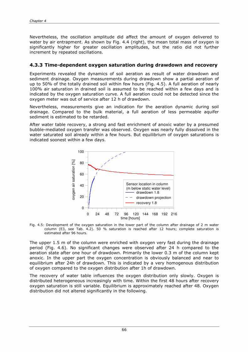
Chapter 4
66
Nevertheless, the oscillation amplitude did affect the amount of oxygen delivered to water by air entrapment. As shown by Fig. 4.4 (right), the mean total mass of oxygen is significantly higher for greater oscillation amplitudes, but the ratio did not further increment by repeated oscillations.
Time-dependent oxygen saturation during drawdown and recovery 4.3.3
Experiments revealed the dynamics of soil aeration as result of water drawdown and sediment drainage. Oxygen measurements during drawdown show a partial aeration of up to 50% of the totally drained soil within few hours (Fig. 4.5). A full aeration of nearly 100% air saturation in drained soil is assumed to be reached within a few days and is indicated by the oxygen saturation curve. A full aeration could not be detected since the oxygen meter was out of service after 12 h of drawdown.
Nevertheless, measurements give an indication for the aeration dynamic during soil drainage. Compared to the bulk material, a full aeration of less permeable aquifer sediment is estimated to be retarded.
After water table recovery, a strong and fast enrichment of anoxic water by a presumed bubble-mediated oxygen transfer was observed. Oxygen was nearly fully dissolved in the water saturated soil already within a few hours. But equilibrium of oxygen saturations is indicated soonest within a few days.
Fig. 4.5: Development of the oxygen saturation in the lower part of the column after drainage of 2 m water column (E3, see Tab. 4.2). 50 % saturation is reached after 12 hours; complete saturation is estimated after 96 hours.
The upper 1.5 m of the column were enriched with oxygen very fast during the drainage period (Fig. 4.6). No significant changes were observed after 24 h compared to the aeration state after one hour of drawdown. Primarily the lower 0.3 m of the column kept anoxic. In the upper part the oxygen concentration is obviously balanced and near to equilibrium after 24h of drawdown. This is indicated by a very homogenous distribution of oxygen compared to the oxygen distribution after 1h of drawdown.
The recovery of water table influences the oxygen distribution only slowly. Oxygen is distributed heterogeneous increasingly with time. Within the first 48 hours after recovery oxygen saturation is still variable. Equilibrium is approximately reached after 48. Oxygen distribution did not altered significantly in the following.
0 24 48 72 96 120 144 168 192 216time [hours]
0
20
40
60
80
100
oxyg
en a
ir s
atu
ratio
n [
%]
Sensor location in column(m below static water level)
drawdown 1.8
drawdown projection
recovery 1.8

Quantifying air entrapment and oxygen uptake from oscillating water tables in column experiments
67
Fig. 4.6: Development of oxygen saturations in the column during an oscillation interval with 24h drainage and 216h recovery.
Conclusions 4.4
Aeration tests point to a downward shift of oxygen by repeated oscillations as result of an oxygen dissolution and an advective transport of dissolved oxygen inside the column. Oxygen entered the drained pores in the water unsaturated zone during drawdown and remained there in strongly enriched concentrations after water table recovery. A downward propagation of oxygen into the permanent water saturated zone was not observed within an oscillation interval of less than 24h. Such repeating short-termed oscillations lead to an enrichment of oxygen, but with a constantly decreasing increment per oscillation.
The time required for a full drainage of the water-saturated soil during well operation is controlled by the sediment characteristics. The aeration tests with a well-sorted middle sand revealed that full drainage and aeration of the sediment may take several days. An aeration up to 50% oxygen air saturation is reached within several hours of drawdown. The dissolution of entrapped air at idle recovery of water table is more rapid (minutes), but equilibrium needs several days to evolve.
By transferring column experiment results on oxygen delivery dynamics to well operation issues, it can be conclude that
- If wells are operated intermittently, the oxic zone in groundwater is significantly more distinct, compared to a situation, where oxygen is only delivered by diffusion to the groundwater. This scenario rarely appears, because water tables vary constantly in managed and exploited aquifers
- Short-termed switching intervals less than 6 to 12 did not enhance the oxygen delivery to groundwater in a relevant extent
- The downward propagation of oxygen bubbles by oscillating water tables into deeper zones of the phreatic aquifer seems to be of minor importance for the oxygen transport. The advective transport of dissolved oxygen might be the major transport process.
Chapter 4
68
- The higher the amplitude of drawdown, the higher the amount of delivered oxygen towards the phreatic zone
- At single switching events, the magnitude of the oscillation amplitude might also impact the concentration of oxygen within the water level oscillation zone as consequence of higher pressures and therefore of increased gas solubility.

Impact of water abstraction on the source and distribution of dissolved oxygen in wells – a field site study
69
Chapter 5
Impact of water abstraction on the
source and distribution of dissolved
oxygen in wells – a field site study
Introduction 5.1
The presence of oxygen in groundwater abstracted by wells and used for drinking water supply crucially affects the water quality as well as the water quantity. The oxygen content controls redox conditions and therefore retardation processes of contaminants in the groundwater. Furthermore, a loss of well performance resulting from the formation of iron incrustations clogging screen and filter pack relies on the amount of oxygen in groundwater.
Oxygen delivery to an anoxic aquifer may result from different processes. Oxygen can delivered to the groundwater by diffusion through the water unsaturated soil or by percolating oxic rain water. Recently two additional pathways attract attention in this context. Air entrapment and dissolution caused by fluctuating water tables and the infiltration of oxic surface water into phreatic aquifers in managed aquifer recharge (MAR) systems.
Due to the abstraction of groundwater by wells, groundwater surface oscillations with highly elevated frequency and amplitude in contrast to natural conditions occur. Many studies already described the entrapment of air and the bubble-mediated gas transfer in water saturated porous media due to oscillating water tables (FAYBISHENKO 1995, FRY et al. 1995, FRY et al. 1996, WILLIAMS & OOSTROM 2000, HOLOCHER et al. 2003). At most natural and artificial recharge sites oxygen is consumed by the biodegradation of organic matter subsequent to the infiltration in the organic rich beds. Thus, the redox state of the infiltrate mainly depends on organic matter loads, temperature, hydraulic connection to the groundwater and infiltration velocities (VON GUNTEN et al. 1991, BOURG & BERTIN 1993, FRITZ 2002, GRESKOWIAK et al. 2005, MASSMANN et al. 2008). On the flow paths towards the abstracting well, re-aeration of the shallow groundwater was observed at several bank filtration well sites (JACOBS et al. 1988, BOURG & BERTIN 1993, MASSMANN et al. 2008, MASSMANN & SÜLTENFUß 2008) and is often ascribed to fluctuating water tables caused by water abstraction from the associated aquifer. A widening of the vertical redox zonation towards the well was observed at a bank filtration site in Berlin (MASSMANN et al. 2008). At this site, infiltration of oxic surface water in winter can additionally lead to a delivery of dissolved oxygen into groundwater contiguous to the banks (GRESKOWIAK et al. 2005, MASSMANN et al. 2008).
All these findings highlighted the importance of adapted well management strategies for a sustainable drinking water supply from aquifers, especially those including MAR systems.
The fact, that only a few studies investigated the oxygen input and distribution in groundwater in detailed temporal and spatial dimensions can be explained by the absence of high-resolution in-situ detection devices for oxygen. Routine sampling of dissolved oxygen is limited to conventional measurements at the well head, which give only mean values for the abstracted water. Additionally, such measurements in an atmospheric environment are vulnerable to outside influences and therefore limited in their reliability.

Chapter 5
70
Several years ago, fiber-optic sensors were developed for the measurement of oxygen in microbiological and medical applications (KLIMANT et al. 1995). This approach was further developed, adapted and tested for the application in hydrogeological contexts (HECHT & KÖLLING 2001, HECHT & KÖLLING 2002). In-situ oxygen measurements with fiber-optic sensors were already applied in field site studies for the investigation of interrelations of hydraulic and hydro-chemical conditions at an artificial recharge pond site (GRESKOWIAK et al. 2005). This sampling method enables the in-situ detection of oxygen down to trace concentrations in greater depth of the aquifer. The measurement itself thereby does not depend on water saturation or other soil physical characteristics and is applicable from the ground surface through the vadose zone down to deeper aquifer zones.
This study is therefore aiming on the assessment of the oxygen delivery to anoxic groundwater with regard to different well operation schemes.
On the basis of field site investigations performed at two-dimensional monitoring networks, equipped with fiber-optic sensors (optodes), oxygen delivery to and distribution in aquifers can be determined wide scaled for the first time. Three well sites in Berlin with different hydrogeological settings and different recharge conditions are chosen for the construction of the monitoring networks. The oxygen enrichment due to groundwater oscillations and oxic infiltration through banks is mainly focused, since these processes are assumed as most important oxygen delivery processes (KOHFAHL et al. 2009).
The impact of both processes on the well performance under various hydraulic and seasonal boundary conditions can then be evaluated. Acquired results can provide knowledge for a general estimation of well clogging potentials and shall help establishing a classification of wells with regard to their clogging vulnerability. Furthermore, the development of an adapted well management strategy shall support the reduction of ochre formation in drinking water wells.
Study sites 5.2
Selection of test sites 5.2.1
As it is known from several studies dealing with well ageing (HANNAPEL 2003, SCHWARZMÜLLER et al. 2009, HOUBEN & WEIHE 2010, VAN BEEK 2010, BUSTOS MEDINA et al. 2013), particularly with clogging processes related to iron incrustations, investigations should focus on the delivery and transport mechanism of main supplies and their derived implications for well management. The dominant enrichment processes and at Berlin well sites are air entrapment by groundwater surface oscillations due to well switching and the relation between recharge and mixing conditions and clogging tendency (KOHFAHL et al. 2009).
Thus, for representative conclusions with regard to Berlin water wells, the study have to consider the mixing conditions of three main water types, which can be distinguished according to their recharge source. These are (i) bank filtrate (BF), (ii) artificial recharged groundwater (AR) and (iii) naturally recharged deep and shallow groundwater (GW). Air entrapment is mainly expected at well sites situated in uncovered and hydraulically unconfined aquifers.
Beside the two main site criteria, aquifer type and mixing conditions, further well site characteristics are regarded. To provide transferability of the empirical investigations at the chosen well sites to the more than 600 other wells in Berlin and also to wells with similar boundary conditions worldwide, the well selection regards the most common well characteristics.

Impact of water abstraction on the source and distribution of dissolved oxygen in wells – a field site study
71
Thus, transect wells should provide following key characteristics concerning:
� Well design:
- stainless steel wire-wound screen, 400 mm diameter
- a maximum depth of 40 m to provide applicability of in-situ oxygen
measurements with optodes
- equipped with electromagnetic flowmeter
� Hydrogeology:
- unconfined hydraulic conditions
- varying shares of groundwater, bank filtrate and artificial recharged water
� Water quality
- comparatively high Nitrate concentrations
- comparatively low Fe(II)-concentrations
� Well operation
- no operational limitations, e.g. permanently operating wells
- mean discharge rates between 50 and 150 m3/h
- mean monthly operational hours between 105 and 560
� Accessibility - Permission for monitoring well construction in the drinking water protection
zone
- Accessibility for drilling rig and monitoring
After analysis of existent well data with regard to the chosen criteria, three well sites are found, who meet most of the claimed requirements. Well selection criteria and characteristics of chosen test sites are given by Tab. 5.1.
Tab. 5.1: Well site criteria for test site selection and compliance by chosen wells (GW=groundwater, BF=bank filtrate, AR=artificial recharge). For main ions see App. 3
Well site criteria Well 15 Well 18 Well 22
Well
desig
n
Filter screen material PVC slot Stainless steel wire wound Stainless steel wire wound
Maximum well depth 16 39 35
Electromagnetic flowmeter No Yes No
Hydro
geolo
gy
Hydraulic condition Unconfined Unconfined Unconfined
Aquifer conductivity 10-4 to 10-5 m/s 10-4 to 10-5 m/s 10-4 to 10-6 m/s
Recharge sources GW, ‘old’ BF ‘old’ BF, AR, GW ‘young’ BF, GW
Wate
r
qualit
y
Mean Fe(II) 1.8 mg/l 0.6 mg/l 1.1 mg/l
Mean NO3 0.7 mg/l 1.8 mg/l 1.1 mg/l
Opera
tion
Mean monthly discharge ~41600 m3 ~35000 m
3 ~50000 m
3
Mean discharge rate ~80 m3/h ~90 m
3/h ~83 m
3/h
Mean monthly operational hours ~525 ~390 ~600
Mean monthly switching frequency 5.1 1.7 3.4
For an evaluation of the influence of different groundwater types on well clogging, three well sites are selected for the construction of monitoring networks. One well has evidently high shares (> 70%) of young (months) riverbank filtrate (FRITZ 2002), one

Chapter 5
72
well has presumably high shares of mid-age to old riverbank filtrate (years) and one well has presumably high shares of artificial recharged groundwater and old riverbank filtrate.
To provide a reliable data basis for the determination of significant hydro-chemical and hydraulic processes in groundwater and well and for the assessment of the well clogging potential, selected well sites were monitored for one hydrological cycle. The monitoring was performed with regard to seasonal variations of hydro-chemical and hydraulic conditions. Additionally, a depth-dependent monitoring was done at the multilevel observation wells. Results and conclusions of this monitoring will be published to a later time. Within this thesis, analysis results of abstracted well water are only consulted to characterize wells generally and reliably.
To provide this, sampling of selected wells was done with the maximum accuracy. Samples were taken after stabilization of in-situ measured physico-chemical parameters. Monitoring of a set of 21 drinking water wells in Berlin, revealed that conditions are stable soonest after 90 min of abstraction, but latest after several hours (see also 2.4). In most of the wells dissolved oxygen is absent after stabilization and redox potentials are far below the mean value of all 678 analysed wells.
Test site Well 15 5.2.2
Location and hydrogeological conditions 5.2.2.1
Well 15 is located in the north of Berlin, adjacent to the Oder-Havel-Channel (see Fig. 5.1). The studied production well is part of a well field of 20 production wells situated along the channel. Distance to the channel is about 150 m and to the proximate neighbored wells 50 m to the north and respectively 100 m to the south. The well was constructed in 1990 and is situated in an unconfined sandy aquifer. The aquifer thickness at the well site is about 16 m and varies between 8 to 24 m laterally. A less permeable marl layer with up to 40 m thickness forms the aquifer basis and limits hydraulic interaction with underlying aquifers.
Under natural flow conditions, the aquifer shows effluent seepage. Due to the high discharge for drinking water production the effluent condition changes to influent (HANNAPEL 2003). Because of the nearby Oder-Havel-Channel a mixing of groundwater and bank filtrate in the well is assumed (HANNAPEL 2003, SCHWARZMÜLLER et al. 2009). Stable isotope data of D and 18O indicate a bank filtrate/groundwater ratio of 2:1 in the abstracted well water.
Fig. 5.1: Site map of well 15 with location of the well field and the monitoring wells.
Hydrochemistry of abstracted water 5.2.2.2
Hydrochemistry of abstracted well water was analysed 6 times between the years 1996 and 2008. Analysis of main chemical compounds in water abstracted by well 15 identified a composition characteristic for the water work with high Ca and HCO3 concentrations, only minor concentrations of Cl and Na and a low total mineralization, compared to the

Impact of water abstraction on the source and distribution of dissolved oxygen in wells – a field site study
73
entity of all abstracted well waters. Hydro-chemical conditions and parameter, crucial for iron-related well clogging processes, show divergent clogging potential tendencies (Fig. 5.2). Comparatively high concentrations of dissolved oxygen (0.06 mg/l) and nitrate (0.7 mg/l) are in opposition to comparatively low redox potential (20 mV) and high dissolved iron concentrations (1.8 mg/l).
Fig. 5.2: Box plots of the most relevant parameters at well 15 with regard to redox conditions and ochre formation.
Well performance 5.2.2.3
Data basis of well 15 provide information about the well performance for the first 16 years of operation. Assessment of specific well yield Qs was regularly done before and after rehabilitation activities. Recently, well yield is around 80% of the initial value (11.3 m3/h/m per meter screen). Two rehabilitations, the first 8 years after construction, the second 5 years later, restored the well yield from 65% to 90% each time successfully. Mean values of entrance resistivity dh are varying for the entire well life on a very low level between 0 and 0.06 m and are obviously not affected by rehabilitations. The development of well performance for well 15 is shown by Fig. 5.3.
The flowmeter profile identifies the lower 40% of the screened well section as most significant influx section with 70% of the total discharge. The upper 20% of the screen contribute around 20% to the total influx, the intermediate section only 10%.
Visual surveillance of the well interior by tv-inspection reveals a directional depth-dependent distribution of deposits (see also App. 4). Deposits in the well mainly occur below the pump downwards to the top of the filter screen. The distribution pattern is obviously consistent with the flow paths of inflowing water. The distribution anisotropy is documented by deposits extended towards the central screen section in only one direction. An assignment of directed deposits to the source of influx - bank filtrate or groundwater - is not possible, because the surveillance video includes no directional information.
600
610
620
630
640
650
EC_µS/cm
n=6
7.4
7.44
7.48
7.52
7.56
pH
n=6
-50
0
50
100
Eh_mV
n=4
0
0.01
0.02
0.03
0.04
0.05
NO2-_mg/l
n=5
1.5
2
2.5
3
3.5
NH4-_mg/l
n=5
1.5
1.75
2
2.25
Fe2+_mg/l
n=6
0.2
0.25
0.3
0.35
Mn2+_mg/l
n=6
0
0.4
0.8
1.2
1.6
NO3-_mg/l
n=5
4.5
5
5.5
6
6.5
DOC_mg/l
n=5
-0.05
0
0.05
0.1
0.15
O2_mg/l
n=4

Chapter 5
74
Fig. 5.3: Development of well performance including rehabilitation measures (left) and influx distribution from Flowmeter at well 15 (right).
Test site well 18 5.2.3
Location and hydrogeological conditions 5.2.3.1
Well 18 is located in the north-western part of Berlin, near the Lake Tegel and the Hohenzollern-Channel (see Fig. 5.4). Well 18 is part of a well field with 22 production wells situated along the Hohenzollern-Channel. Distance to the channel is about 200 m and about 210 m to the Lake Tegel, but bank filtration is only taking place at the banks of Lake Tegel. The bed of the artificial Hohenzollern-Channel is sealed. Additionally to the lake and the channel, three artificial recharge ponds are situated close to the well field and are surrounded triangular by the well field. The nearest pond is located in 150 m distance to the well. Distance to the proximate neighbored wells is 50 m to the north and south.
The well was constructed in 2008 and is situated in an unconfined sandy aquifer, whose thickness at the well site is about 40 m and varies between 35 to 45 m laterally. A lower less permeable marl layer with up to 40 m thickness prevents short termed interaction with underlying aquifers.
The filter screen of the studied well is separated into two sections, which penetrate the aquifer from 20 to 31 m and from 33 to 39 m depth. Because of the infiltration of surface water at the banks of Lake Tegel and of the artificial recharge pond a mixing of bank filtrate, groundwater and artificial recharged water in the well can be assumed.
Fig. 5.4: Site map of well 18 with location of the well field and the monitoring wells.
0 2 4 6 8 10 12 14 16Well age [years]
0
25
50
75
100W
ell
cap
acity Q
s [
%]
0
0.5
1
1.5
En
tra
nce
re
sis
tan
ce
∆h
[m
]
Qs
∆h
Regeneration
0 20 40 60 80 100
Discharge [%]
100
80
60
40
20
0
Filt
er
scre
en [
%]
Flow meter after constructionDischarge rate: 46 m3/hTotal screen length: 6 m

Impact of water abstraction on the source and distribution of dissolved oxygen in wells – a field site study
75
Hydrochemistry of abstracted water 5.2.3.2
Hydrochemistry of abstracted well water was analysed 6 times between the years 2008 and 2011. Analysis of main chemical compounds in water abstracted by well 18 identifies a composition characteristic for the water work with a comparatively higher fraction of Na and Mg, but with comparatively median concentrations of Cl, SO4 and HCO3. Total mineralization is slightly below the median of all abstracted well waters. Hydro-chemical conditions and parameter, crucial for iron-related well clogging processes, show a relatively consistent clogging potential tendency (Fig. 5.5). Compared to the entity of wells, abstracted water of well 18 contains significantly high concentrations of nitrate (1.9 mg/l) and significantly low concentrations of dissolved iron (0.5 mg/l). Oxygen is completely depleted in abstracted water. The redox potential (35 mV) varies only slightly and is in the median range of all other wells. Thus, well 18 apparently possess a distinct clogging potential based on redox conditions and availability of reactants, respectively nutrients.
Fig. 5.5: Box plots of the most relevant parameters at well 18 with regard to redox conditions and ochre formation.
Well performance 5.2.3.3
Data basis of well 18 provide only 3 years (2008-2011) of information about the well performance. Assessment of specific well yield Qs was done two times since well construction. The well yield has decreased to already 60% of the initial value (4.7 m3/h/m per meter screen) within three years of operation. The well was not rehabilitated so far. In contrast to the specific well yield, entrance resistivity dh was not increasing throughout the past (Fig. 5.6).
The flowmeter profile identifies the upper 10% of the screened well section as most important influx section with 40% of the total discharge. Below the highly productive section at the screen top, influx is distributed homogeneous down to the cased section. This section contributes another 50% to the total discharge. Only 10% are allotted to the 6 m of the lower filter screen. Thus, nearly the total influx is restricted to the upper filter screen with a length of 11 m (Fig. 5.6).
TV-inspection of well 18 was not available up to the time of publication. Decrease in well yield and high screen entrance velocities at the top of filter screen suggests an appearance of deposits inside the well.
680
700
720
740
760
780
EC_µS/cm
n=5
2.5
3
3.5
4
4.5
5
5.5
DOC_mg/l
n=5
0
1
2
3
4
NO3-_mg/l
n=6
0.2
0.4
0.6
0.8
1
Mn2+_mg/l
n=6
0.4
0.6
0.8
1
Fe2+_mg/l
n=6
0.2
0.4
0.6
0.8
1
NH4-_mg/l
n=5
0
0.1
0.2
0.3
0.4
0.5
NO2-_mg/l
n=5
10
20
30
40
50
60
Eh_mV
n=5
7.35
7.4
7.45
7.5
pH
n=5
-0.04
-0.02
0
0.02
O2_mg/l
n=6

Chapter 5
76
Fig. 5.6: Development of well performance including rehabilitation measures (left) and influx distribution from Flowmeter at well 18 (right).
Test site well 22 5.2.1
Location and hydrogeological conditions 5.2.1.1
Well 22 is located in the southeast of Berlin at the western shore of Lake Müggel (see Fig. 5.7). Well 22 is part of a well field with 24 vertical wells situated along the lake bank. Distance from well 22 to the lake is about 70 m, to the neighbored well in the south 50 m and in the north 70 m, respectively. The well site was constructed in 2004. The well is situated in an unconfined sandy aquifer. The aquifer thickness at the well site is 35 m and varies laterally from 30 to 40 m. The aquifer is separated by less permeable marls from underlying aquifers. Well 22 is screened in medium to coarse sands from 20 to 34 m depth.
The occurrence of saline groundwater in deep observation wells indicates a localized hydraulic connection of the fresh water aquifer complex and the underlying salt water formation. FRITZ (2002) calculated mixing ratios for the well field based on time series of strontium (Sr), chloride (Cl) and sodium (Na). Results indicate shares of 72 % bank filtrate, 23 % groundwater and 5 % deep groundwater. Furthermore the assessment of travel times for bank filtrate, determined by hydraulic parameter and temperature along an observation well transect, revealed an incipient colmation of the bank in this lakeshore area with flow velocities of one to two m per day.
Fig. 5.7: Site map of well 22 with location of the well field and the monitoring wells.
Hydrochemistry of abstracted water 5.2.1.2
Hydrochemistry of abstracted well water was analysed 7 times between the years 2004 and 2010. Analysis of main chemical compounds in water abstracted by well 22 identifies a composition characteristic for the water work with comparatively usual fractions of Ca,
0 1 2 3Well age [years]
0
25
50
75
100W
ell
cap
acity Q
s [
%]
0
0.5
1
1.5
En
tra
nce
re
sis
tan
ce
∆h
[m
]
0 20 40 60 80 100
Discharge [%]
100
80
60
40
20
0
Filt
er
scre
en
[%
]
Casing
Flow meter after constructionDischarge rate: 34 m3/hTotal screen length: 19 m

Impact of water abstraction on the source and distribution of dissolved oxygen in wells – a field site study
77
Na and Mg, but with comparatively high concentrations of SO4 and low HCO3 concentrations. Total mineralization is in the median range compared to the entity of abstracted well waters. Hydro-chemical conditions and parameter, crucial for iron-related well clogging processes, show a relatively consistent clogging potential tendency Fig. 5.8). Abstracted water contains traces of dissolved oxygen (0.02 mg/l), comparatively high nitrate (0.7 mg/l) and low dissolved iron (1.1 mg/l) concentrations. Only redox potential is with 20 mV low compared to the bulk of wells and indicates a minor clogging potential. Though, well 22 apparently possess a distinct clogging potential considering redox conditions and availability of reactants, respectively nutrients.
Fig. 5.8: Box plots of the most relevant parameters at well 22 with regard to redox conditions and ochre formation.
Well performance 5.2.1.3
Data basis of well 22 provide information about the well performance for the first 8 years of operation between 2004 and 2012. Assessment of specific well yield Qs was done increased during the last 3 years. A single rehabilitation 6 years after construction restored the capacity about 12% from 66% to 78% of the initial well yield (3.6 m3/h/m per meter screen). Since then, specific yield decreases again to 65% within two years. Values of screen entrance resistivity are increasing throughout the well life and up to 0.45 m. First maintenance activities after 6 years rehabilitate well losses almost completely, but not with sustained success. Similar to well yield, entrance resistivity recovered to the pre-rehabilitation state within a year (see Fig. 5.9).
The flowmeter profile identifies the upper 10% of the screened well section as most important influx section with 40% of the total discharge. A second important influx zone with 30% of total discharge allotted to 1.5 m screen length in the central screen section. Below both highly permeable sections, influx is significantly lower. In summary, it can be stated that upper and lower half of the screen contributes nearly the same portion of influx to total discharge (see Fig. 5.9).
Visual surveillance of well 22 by a tv-inspection revealed a clear directional and depth-dependent distribution of deposits (see also App. 5). Deposits mainly occur at the top of filter screen, whereas only one side of the well interior is affected. The application of a directed tv-inspection allows the correlation of affected zones with the sources of well recharge. Thus, the most affected zone is directed towards the lake. Zones directed towards neighbored wells show considerable deposits as well. Only the landward oriented zone is visually free from deposits.
720
760
800
840
880
920
EC_µS/cm
n=6
7.3
7.4
7.5
7.6
pH
n=6
-20
0
20
40
60
80
Eh_mV
n=5
0
0.005
0.01
0.015
0.02
0.025
NO2-_mg/l
n=6
0
0.2
0.4
0.6
0.8
NH4-_mg/l
n=6
1
1.1
1.2
1.3
Fe2+_mg/l
n=7
0.4
0.5
0.6
0.7
0.8
Mn2+_mg/l
n=7
0
0.5
1
1.5
2
2.5
NO3-_mg/l
n=7
4
4.4
4.8
5.2
5.6
DOC_mg/l
n=5
-0.05
0
0.05
0.1
0.15
O2_mg/l
n=7

Chapter 5
78
Fig. 5.9: Development of well performance including rehabilitation measures (left) and influx distribution from Flowmeter at well 22 (right).
Methods and materials 5.3
Experimental design 5.3.1
To quantify the impact of well operation on the oxygen delivery to the well at the three selected well sites several pumping tests were carried out under various boundary conditions.
A first pumping test were performed to measure short-term impacts during an abstraction period of 24 h. The initial phase of of operation and recovery were of special interest during this single well switching event.
A second pumping test aimed at mid-term variations of oxygen transport during an period of continuous abstraction of at least one week. Results should reveal how temporally stable the distribution of oxygen is and to what extent oxygen delivery may change during extended abstraction phases.
A third operation pattern of interest is the hydraulic interference of wells and how those interferences between neighbored wells affect the oxygen distribution.
These three operational events and their monitoring are described in the following. Events and their boundary conditions are also summarized and presented in Tab. 5.2.
Single well switching events 5.3.1.1
In the first phase of investigations, wells abstracted water for a period of 24 hours. This test represents short-timed switching intervals. Monitoring of oxygen and hydraulic heads starts 24 hours prior to abstraction and ends after 24 hours of recovery until initial conditions are mostly re-established.
As already mentioned, in unconsolidated aquifers the process of well screen clogging is generally controlled by the hydraulic conditions in the well and the adjacent aquifer. Particularly with regard to wells and their operation schemes, hydraulic conditions in the aquifer are varying strongly and thus affect the oxygen distribution and therefore clogging rates. According to VAN BEEK et al. (2009) the act of water abstraction can be divided into four main phases: (i) idle equilibrium, (ii) initial abstraction, (iii) abstraction equilibrium and (iv) idle recovery. This concept is applied to the monitoring of oxygen and adapted to the conditions prevailing at Berlin well sites:
(i) idle equilibrium
To provide the idle equilibrium, investigated wells and the four proximate neighbored wells were shut down at least one week prior to the pump test.
0 1 2 3 4 5 6 7 8Well age [years]
0
25
50
75
100W
ell
cap
acity Q
s [
%]
0
0.5
1
1.5
En
tra
nce
re
sis
tan
ce
∆h
[m
]
Regeneration
0 20 40 60 80 100
Discharge [%]
100
80
60
40
20
0
Filt
er
scre
en
[%
]
Flow meter after constructionDischarge rate: 36 m3/hTotal screen length: 14 m

Impact of water abstraction on the source and distribution of dissolved oxygen in wells – a field site study
79
(ii) initial abstraction
As identified by a preliminary study of hydro-chemical conditions in the abstracted well water at 22 selected wells, the abstracted water is almost in thermo-dynamic equilibrium after 2-3 hours of continuous abstraction. Main solutes as well as redox sensitive parameters had stabilized within this time (see also chapter 2.4), which represents the initial abstraction phase.
(iii) abstraction equilibrium
After 2-3 hours of abstraction, abstraction equilibrium follows and was observed for at least 20 hours of continuous abstraction.
(iv) idle recovery
Concordant to the shutdown of abstraction, recovery of water table begins. The recovery of the water table and the refill of the depression cone approximately correspond to the time, which is needed until abstraction equilibrium is reached. Taking into account the process of air entrapment and bubble-mediated gas transfer, the recovery phase was observed for at least 24 hours.
Continuous abstraction 5.3.1.2
As results of simulated oxygen transport indicate, travel times of shallow oxic water or respectively oxic bank filtrate to the well are in the range of weeks. This longer termed migration of oxic species in groundwater has to be considered by extending the observation period.
Thus, oxygen distribution and hydraulic heads were additionally observed before, during and after an extended period of continuous abstraction of at least one week. Hydraulic conditions in the well near aquifer were tried to keep stable during the tests, e.g. neighbored wells were not switched.
Well interference between neighboring wells 5.3.1.3
Water abstraction from an aquifer causes a decrease of the water table by creating a cone of depression. In well fields with a close-meshed well grid, depression cones of neighboured wells may interfere. This interference reduces the water supply, wells compete for the same water and withdrawal decreases. Further, the formation of a cone of depression increases the hydraulic gradient in the affected aquifer and flow is accelerated. This may also lead to an enhanced migration of oxic water at wells, which are located in the depression cone of a neighboured well, but resting themselves.
The assessment of the influence of interacting wells on oxygen delivery includes a four-week test phase. During this phase, neighboured wells are operated in varying constellations, while the test well itself rests throughout the entire four weeks. After one week with static hydraulic conditions, one proximate neighbour well abstracts water for one week. Afterwards, all wells are shutdown to provide re-establishment of initial hydraulic conditions. Then, both proximate neighbour wells start to abstract for one week.

Chapter 5
80
Tab. 5.2: Boundary conditions of monitoring events at wells 15, 18 and 22.
Monitoring event Single well
switching
Continuous
abstraction
Well
interaction
Well 15
Operation [h] 24 168 -
Resting duration prior to event [h] 1779 42 44
Oxygen monitoring [h] 119 338 340
Initial water level [masl] 31.5 31.2 31.5
Maximum drawdown in well [m] 1.9 1.2 -
Sampling month Oct. Dec. Feb.
2nd proximate well south resting resting resting
1st proximate well south resting resting resting
1st proximate well north resting resting operating
2nd proximate well north resting resting resting
Well 18
Operation [h] 24 51 166 -
Resting duration prior to event [h] 126 171 164 643
Monitoring of oxygen [h] 118 51 408 667
Initial water level [masl] 28.2 28.1 28.0 28.5
Maximum drawdown in well [m] 1.5 1.1 1.4 0.5
Sampling month Jun. Jul. Jan. Nov.
2nd proximate well east operating resting operating resting
1st proximate well east resting resting resting operating
1st proximate well west resting resting resting operating
2nd proximate well west operating resting resting resting
Well 22
Operation [h] 35 26 360 -
Resting duration prior to event [h] 163 171 143 345
Monitoring of oxygen [h] 95 167 508 453
Initial water level [masl] 31.3 31.5 31.5 31.6
Maximum drawdown in well [m] 2.4 - 2.7 0.8
Sampling month Jun. Sept. Sept. Oct.
2nd proximate well north resting resting resting operating
1st proximate well north resting operating resting operating
1st proximate well south resting operating resting operating
2nd proximate well south operating operating operating resting
Monitoring network design 5.3.2
Regarding the purpose of field site studies and the experimental design, the chosen well sites were equipped with a bidirectional transect of multilevel observation wells. To achieve a high spatial resolution of the oxygen distribution in the cone of depression, the monitoring network was installed as close as possible to the wells (at least one multilevel observation well in 3 m distance to the abstraction well). The orientation of the observation wells allows a hydro-chemical and hydraulic monitoring of main inflows, e.g. bank filtrate and groundwater. The monitoring networks, installed at the three well sites,

Impact of water abstraction on the source and distribution of dissolved oxygen in wells – a field site study
81
differ in their orientation and their resolution, according to the specific hydrogeological and constructional site settings. For specific setup information see Fig. 5.10.
The installation of optodes for in-situ measurement of oxygen was done concomitant to the installation of multilevel wells. Optodes were attached to the piezometer casing from the outside. The interval and number of installed optodes is site specific and is determined by analysis of hydraulic tests.
The chosen setup should provide information about the delivery and distribution of oxygen along the flow paths towards the screened section of the production well. As mentioned before, it is assumed that oxygen is mainly delivered to groundwater by water level oscillations and is then advectively transported towards the well along the gradient. Therefore, location of static and dynamic water levels is the decisive criteria for the placement of optodes in the upper aquifer zone. The most upper optode should provide information about the oxygen saturation in the vadose zone, under permanently water unsaturated conditions, because soil air is the reservoir for re-aerating the cone of depression once abstraction has started. The specific depth-dependent location of the most upper optode was determined considering the water level development during the last five to ten years and regarding seasonal and climatic effects and recent and former operational conditions (discharge rates and number of operating wells in the well field). Thus, the optode was installed above the maximum measured water level including the capillary fringe. The closest interval of optodes is located in the zone corresponding to the maximum amplitude of water level oscillations. Additional optodes were placed in depths corresponding to the flow paths directing to the top and center of the screened well section and one optode was placed at the bottom of the well screen to represent the oxygen free endmember of the mixing line.
Additionally to the optodes in the aquifer, a string of optodes was temporarily placed in the well interior to detect oxygen with regard to its depth-dependent appearance. The string was equipped with five optodes in depth corresponding to the pump inlet and the well screen, particularly its top and bottom.
Fig. 5.10: Setup of the monitoring networks at wells 15, 18 and 22 including piezometer (P) and oxygen sensors (O) in aquifer and inside the well (see App. 6 and App. 7).
Monitored parameter 5.3.3
Oxygen 5.3.3.1
For the detection of oxygen, fiber-optical oxygen sensors, also known as optodes were used. The measuring principle of the optodes is based on the effect of dynamic luminescence quenching by molecular oxygen (PRESENS 2006).

Chapter 5
82
For the field application, optodes basing on 2 mm polymer optical fibers (POF) were constructed manually. Calibration of optodes was performed using a two-point calibration in oxygen-free water (cal0) and water vapor saturated air (cal100) (HECHT & KÖLLING 2001, HECHT & KÖLLING 2002, PRESENS 2006). Optodes were calibrated under laboratory conditions. The POF were connected by a SMA fiber connector to the one-channel fiber-optic oxygen meter Fibox3 (Precision Sensing GmbH). The detection limit of the optodes is given by the used oxygen sensitive sensor in combination with the used oxygen meter. According to PRESENS (2006) the detection limit for the used optodes is 15 ppb or respectively 0.03 % air saturation in the range from 0 - 100 % oxygen. The accuracy of measurement depends on the components used for optode construction and on the oxygen saturation. Length of optical fibers has a significant impact on the signal quality (amplitude) and on the precision of measurement, too. The influence of the cable length on the transmission loss of the constructed optodes is considerably increasing for cable length >20m. Therefore, measurement accuracy is lower for optodes installed in greater depth of the aquifer. To solve this problem, sampling rates are increased to calculate mean values for each sampling interval. Furthermore, the oxygen content has a relevant impact on the accuracy. Due to the fact, that in absence of oxygen, the luminescence signal is much stronger than in presence of oxygen, the measurement is more precise if oxygen is absent or only present in low concentrations. The response time of the oxygen sensors is less than ten seconds for the gas phase and less than a minute for the liquid phase (PRESENS 2006).
To provide long-term monitoring of oxygen saturations in the 2-dimensional setup of the transects at the well sites, an automatic sensor changer based on a printer module was developed corresponding to HECHT and KÖLLING (2001). By this approach, an automatic sampling of up to 40 optodes in series was feasible. The sampling interval of the oxygen measurements varied, depending on the experimental setup, between one and ten seconds and the dwell time varies between 10 and 30 seconds. Accordingly, the sampling interval of each optode was between 15 to 60 minutes.
The values of oxygen air saturations were temperature-compensated with the measured groundwater temperature afterwards. Temperature data were obtained from seasonal hydro-chemical samplings of the multilevel observation wells and from PT-logger installed in the piezometers.
To analyse and interpret the recorded oxygen data, oxygen air saturations were the preferred unit. They provide the best comparability between different monitoring events and different study sites. For a conversion into concentrations the water pressure associated with the installation depth of the optode factors into the calculation. In case of an enrichment of oxygen by water level oscillations and increasing pressures with water depth oxygen air saturations above 100% might be expected. This enrichment is best displayed by using oxygen air saturations instead of concentrations.
Hydraulic heads 5.3.3.2
Hydraulic heads in wells, filter packs and transect wells were determined in varying intervals by measuring the water level with reference to points of known elevation. Automatic water level and temperature logging by PT-probes was done continuously in the well and at least in one of the transect wells.
At Berlin wells, dynamic hydraulic heads and shape of depression cone are not only subject to the actual discharge rate of the well and the hydrogeological characteristics of the exploited aquifer, but also to the operation state of neighbored wells, to water level fluctuations of nearby rivers and lakes and to the operation state of artificial recharge ponds and to their hydraulic connection to the aquifer. Furthermore, the wells of a well field share the same collector pipe system, which causes pressure fluctuations and variations in the wells discharge rates, when single wells are switched on and off. Thus, hydraulic heads vary constantly in minor to considerable scales.

Impact of water abstraction on the source and distribution of dissolved oxygen in wells – a field site study
83
Discharge rate 5.3.3.3
Discharge rates of well 18 were measured by inductive metering and were automatically transferred to the data bank of the operator. Discharge rates of wells 15 and 22 have to be determined manually with a flowmeter installed at the well head.
Impact of well switching events 5.4
Results and discussion 5.4.1
The monitoring of oxygen air saturations in the aquifer close to the well was accompanied by a monitoring of oxygen inside the well in different depth. Throughout the entire sampling period, which includes up to 35 hours of abstraction and 24 hours of recovery, oxygen could not be detected inside the three wells. An appearance of oxygen was expected, if at all, at the uppermost meter of the filter screens and above. Thus, results of the oxygen measurements from the well interior are not shown und discussed explicitly.
Well 15 5.4.1.1
The pump test, at well 15 was performed in autumn and is divided into the four abstraction phases as described above. The idle phase prior to abstraction is characterized by nearly unaffected hydraulic conditions. Due to extended rehabilitation activities at the well field this phase last 10 weeks resulting in a continuous water table rise and a hydraulic change from influent to effluent groundwater conditions. Subsequent to the idle phase, well 15 abstracts water for 24 hours, resulting in a maximum drawdown of the water level inside the well of 1.9 m. The respective hydraulic heads, observed in the piezometers, decrease from 0.8 m in 2.25 m distance to 0.5 m in 5 m distance. According to the piezometric heads, the cone of depression develops nearly homogeneous in both directions (groundwater and bank filtrate). The proximate neighbored wells rest during the pump test. Results of oxygen and piezometer measurements are presented in Fig. 5.11.
Assessment of idle equilibrium conditions reveals a laterally homogeneous distribution of oxygen in the aquifer. Atmospheric conditions, with oxygen air saturations above 90% are observed in the vadose zone of the aquifer. The phreatic zone is generally characterized by the absence of dissolved oxygen.
Additionally, no difference in oxygen distribution is obvious between groundwater and bank filtrate.
Initial abstraction causes a descending water level followed by an aeration of the depression cone, which is expressed by rising oxygen air saturations, as soon as water table drops below the depths of the associated optode.
The transition from initial abstraction to abstraction equilibrium is characterized by strongly increasing oxygen air saturations in the depression cone. An increase of oxygen air saturations in the phreatic zone (1 m below the water table) is observed in all profiles, except distant to the well in groundwater direction.
The appearance of oxic water in the uppermost groundwater layer indicates a descent of the shallow oxic groundwater, as observed at idle equilibrium, with a gradually interface between oxic and anoxic conditions close to the well.
The various oxygen air saturations in the depression cone and the variable aeration behaviour during abstraction suggest a heterogeneous spatial distribution of sediments. A significant influence of small-scale heterogeneities in aquifer sediments on solute transport was already observed in field (GRESKOWIAK et al. 2005) and in laboratory

Chapter 5
84
studies (WANG et al. 2003). The depression cone itself is continuously enriched by oxygen diffusing from soil air.
The retardation in oxygen increase, resulting in a stabilization or depletion of saturations, observed in bank filtrate direction, may be the result of homogeneous oxidization of Fe(II) from anoxic groundwater mixed with oxic groundwater. Oxidation proceeds until one of the reactants is depleted. The development of oxygen air saturation in the shallow groundwater also indicates a depletion of Fe(II), because DO stabilizes with time. The delayed appearance of oxygen in groundwater direction may result from sedimentological heterogeneities in turn.
Fig. 5.11: Temporal development of oxygen saturations in different depths of the aquifer at well 15 during a single switching event. Dotted lines separate the four different abstraction phases idle equilibrium (1), initial abstraction (2), abstraction equilibrium (3) and idle recovery (4).
With idle recovery of the water table, oxygen air saturations decrease significantly in the aquifer. As soon as water table rises above the depths, where optodes are placed, oxygen saturations decrease rapidly. The oxygen degradation rate is comparably similar in all profiles: a rapid drop is followed by a smooth decline until oxygen is fully depleted. The time, needed until full depletion is reached, obviously depends on the maximum oxygen content in the depression cone before the water table recovers.
The stabilization of oxygen air saturation distant to the well in groundwater is consistent with the results of re-oxidization experiments of anoxic water performed in laboratory by WILLIAMS and OOSTROM (2000), who identified oxygen saturation between 50 to 100% after repeated water table fluctuations. A complete dissolution of the oxygen, present in the gaseous phase, would result in oxygen air saturations in water above 100% as calculated by KOHFAHL et al. (2009). But this effect is not observed for the recovery phase of the pump test at well site 15.
The detected rapid decrease of oxygen air saturation in the depression cone after water table re-rise is most likely related to the degradation of oxygen by oxidizing processes. Because the depression cone is refilled not only by vertical ascending groundwater, but mainly by horizontal groundwater flowing towards the well following the hydraulic gradient, the supply by anoxic Fe(II)-bearing groundwater is not sufficiently provided to
0 12 24 36 48Time [h]
0
25
50
75
100
Oxyg
en
air
sa
t. [
%]
28
29
30
31
32
Altitu
de
[m
ab
ove
se
a le
ve
l]
E - 5.00 m to well in GW
1 2 3 4
0 12 24 36 48Time [h]
0
25
50
75
100
Oxyg
en
air
sa
t. [
%]
28
29
30
31
32
Altitu
de [
m a
bo
ve
se
a le
ve
l]
D - 2.25 m to well in GW
1 2 3 4
0 12 24 36 48Time [h]
0
25
50
75
100
Oxyg
en
air
sa
t. [
%]
28
29
30
31
32
Altitu
de
[m
ab
ove
se
a le
ve
l]
A - 2.25 m to well in BF
1 2 3 4
0 12 24 36 48Time [h]
0
25
50
75
100
Oxyg
en
air
sa
t. [
%]
28
29
30
31
32
Altitu
de
[m
ab
ove
se
a le
ve
l]
B - 5.00 m to well in BF
1 2 3 4
O2 - 32 masl
O2 - 31 masl
O2 - 30 masl
O2 - 29 masl
O2 - 26 masl
O2-sensor pos.
hydraulic head
O2 - 32 masl
O2 - 31 masl
O2 - 30 masl
O2 - 29 masl
O2 - 26 masl
O2-sensor pos.
hydraulic head
O2 - 32 masl
O2 - 31 masl
O2 - 30 masl
O2 - 29 masl
O2 - 26 masl
O2-sensor pos.
hydraulic head
O2 - 32 masl
O2 - 31 masl
O2 - 30 masl
O2 - 29 masl
O2 - 26 masl
O2-sensor pos.
hydraulic head

Impact of water abstraction on the source and distribution of dissolved oxygen in wells – a field site study
85
deplete the total oxygen by homogeneous oxidation of Fe(II). Simulations of the bubble-mediated gas transfer from entrapped air under advective flow regime revealed a degradation of the oxygen within 25 hours after oxidization (HOLOCHER et al. 2003). In case of a continuous supply with fresh Fe(II), the time needed for a complete depletion of oxygen decreases significantly. The occurrence of Fe(III)hydroxides and oxides in aquifer sediments in the fluctuation zone, especially close to wells, are the product of this process. But the influence of horizontal flow is limited by the presence of a stagnant flow zone in the upper meter of the phreatic zone, reducing the hydraulic conductivity and enhancing the vertical flow component (RYAN et al. 2000). The fast DO degradation in the depression cone of well 15 additionally bases in all probability on the microbial consumption of oxygen. Though, it has to be regarded, that, caused by the extended period of natural flow conditions prior to the pump test, the aquifer was almost anoxic and oxygen was only delivered to groundwater by diffusion through the vadose zone. Therefore, reduction capacity, in terms of reduced ions available for oxidization by DO is enhanced as long as a constant supply is provided during initial recovery.
Furthermore, the change to effluent conditions results in a relocation of the bank filtrate/groundwater-interface towards the river. During regular well field operation, this interface is located along the axis of the well field. Thus, bank filtrate share in abstracted water and its influence on the oxygen distribution is assumed to be of minor importance during this single switching event.
Well 18 5.4.1.2
The short-pump test at well 18 was accomplished after 120 hours of static hydraulic conditions. Abstraction and recovery duration was 24 hours in both cases. Drawdown of the hydraulic head in well 18 occurs rapidly to a total value of 1.5 m after 24 hours of abstraction. Hydraulic heads measured at the piezometer, screened 13 m below the initial water table, show maximum drawdowns of 0.8 m. The hydraulic gradient was directed towards the artificial recharge pond during the entire pump test. Proximate neighbour wells were resting for the observed time period. Because oxygen was present only in the upper part of the aquifer, measurements of deep groundwater are not displayed in detail. Further, samplings in bank filtrate direction were as well disregarded due to the damage of several designated optodes, including the four most upper sensors. Results of oxygen and piezometer measurements are presented in Fig. 5.12.
Fig. 5.12: Temporal development of oxygen saturations in different depths of the aquifer at well 22 during a single switching event. Dotted lines separate the four different abstraction phases idle equilibrium (1), initial abstraction (2), abstraction equilibrium (3) and idle recovery (4).
At idle equilibrium oxygen distribution shows a distinct zonation in the aquifer directed towards the artificial recharge pond. Almost anoxic conditions are present at idle equilibrium. The presence of dissolved oxygen is limited to the vadose zone, where
0 6 12 18 24 30 36 42 48Time [h]
0
20
40
60
80
100
Oxyg
en
air
sa
tura
tio
n [
%]
23
25
27
29
31
Altit
ud
e [
m a
bo
ve
se
a le
ve
l]
O2 - 31.0 masl
O2 - 29.0 masl
O2 - 27.0 masl
O2 - 25.0 masl
O2 - 23.0 masl
O2-sensor pos.
hydraulic head
H - 3 m to well in AR
1 2 3 4

Chapter 5
86
oxygen is already degraded, which diminishes the potential oxygen delivery by diffusion through the unsaturated soil into the groundwater. Additionally, the availability of oxic soil air for a re-aeration of the depression cone, when water table descends as result of water abstraction, is limited and the oxygen amount potentially entrapped in air bubbles, as water level re-rises, is significantly reduced.
The main factor, controlling the advective transport of gas in the soil and its entrapment, is the permeability of the respective aquifer zone. Sediments in the vadose zone and in the upper phreatic zone at well 18 are mainly fine to medium-grained sands. In medium to coarse sands entrapped air made up to 50% of the pore volume, whereas fine sands are able to retain gas in less than 20% of the pore volume (FRY et al. 1997).
In the phreatic zone itself, oxygen is completely absent.
Once initial abstraction has started, oxygen air saturation increase in the vadose as well as in the upper phreatic zone. But the oxygen enrichment is only limited to a narrow zone in the upper aquifer.
After the initial abstraction phase (3 hours), oxygen air saturation has stabilized in the vadose and the phreatic zone at abstraction equilibrium. Whereas, atmospheric conditions prevail above the water table, groundwater below is nearly completely oxygen-depleted, except of slight oxygen enrichment in 25 masl appearing at the end of the abstraction period. During the abstraction period of 24 hours, variability of oxygen air saturation is generally minor, although the water level still decreases considerably.
The localized appearance of oxygen below shallow anoxic water in AR direction may origin from oxic infiltration at the recharge pond. As observed by GRESKOWIAK et al. (2005), the infiltration conditions and the aeration status of the aquifer below the recharge pond closely correlate with the hydraulic behavior, which is controlled by the filling cycle of the pond and the hydraulic connection between pond and groundwater. Further, aerobe conditions during infiltration and along the flow path, resulting in abstraction of oxic water by a well, requires low infiltration temperatures and short residence time of artificial recharge in the aquifer. Infiltration at the recharge pond was active during summer from April to October and inactive for the rest of the year. The oxygen sampling took place in July after 3 months of continuous infiltration. Thus, the observed conditions in the aquifer at well 18 represent in all probability the case, where artificial recharge plays a minor role and the well is mainly recharged by rain, groundwater and “old” bank filtrate. This is also indicated by the groundwater temperatures, which are measured concurrently to the oxygen sampling and represent with 12°C the average yearly groundwater temperature. A strong influence of artificial recharge on the aquifer would result in significantly higher temperatures, which reflect the high surface temperatures during infiltration in summer.
Shutdown of the well pump results in a rapid water level rise at idle recovery and in a sudden and strong decline of oxygen air saturation in the vadose zone. The phreatic zone is completely oxygen-depleted 6 hours after end of abstraction. 15 hours after abstraction, oxygen air saturation in the soil air close to the water table, begin to re-rise slowly.
Well 22 5.4.1.3
The pump test at well 22 was performed in summer. The idle equilibrium was ascertained after seven days of hydraulic conditions unaffected by operating wells in a spatial range of 100 m. Water table recovers during this time to 31.3 m above sea level. Water abstraction by well 22 results in a drawdown of the water level inside the well to a maximum of 2.4 m after 35 hours. Due to technical limitations the abstraction period has to be prolonged and exceeds the scheduled 24 hours. The respective hydraulic heads, observed in the piezometers in 3 m distance to the well, drop about 0.5 m at the end of abstraction period. Similar drawdown values, observed in bank filtrate and groundwater directed piezometers, indicate an almost homogeneous expansion of the depression cone. After abstraction ends, oxygen air saturations and hydraulic heads are observed for

Impact of water abstraction on the source and distribution of dissolved oxygen in wells – a field site study
87
further 24 hours during the idle recovery phase. Results of oxygen and piezometer measurements are presented in Fig. 5.13.
Fig. 5.13: Temporal development of oxygen saturations in different depths of the aquifer at well 22 during a single switching event. Dotted lines separate the four different abstraction phases idle equilibrium (1), initial abstraction (2), abstraction equilibrium (3) and idle recovery (4).
At idle equilibrium oxygen distribution reveals a sequence from atmospheric to oxic to anoxic conditions in the well near aquifer. The zone with an atmospheric oxygen air saturation includes the vadose zone and the most upper meter of the phreatic zone, in both, groundwater and bank-filtrate direction. Below this zone, oxygen is still enriched down to 16.5 masl in bank filtrate and down to 24.5 masl in groundwater. The deeper aquifer zones below are free of dissolved oxygen.
The occurrence of a nearly oxygen depleted layer in shallow groundwater directly below the zone with atmospheric oxygen air saturation, suggests a layering of anoxic water on top of oxic water in the well-near aquifer. If considered in detail, this anoxic layer is also indicated by a slight, but still obvious depletion of oxygen in bank filtrate direction.
0 6 12 18 24 30 36 42 48 54 60Time [h]
0
20
40
60
80
100
Ox
yg
en
air
sa
t. [
%]
29
30
31
32
29.5
30.5
31.5
Alt
itu
de
[m
ab
ov
e s
ea
le
ve
l]
O2 - 31.5 masl
O2 - 30.5 masl
O2 - 29.5 masl
O2-sensor pos.
hydraulic head
F - 3 m to well in BF
1 2 3 4
0 6 12 18 24 30 36 42 48 54 60Time [h]
0
20
40
60
80
100
Ox
yg
en
air
sa
t. [
%]
29
30
31
32
29.5
30.5
31.5
Alt
itu
de
[m
ab
ov
e s
ea
le
ve
l]
O2 - 27.5 masl
O2 - 26.5 masl
O2 - 24.5 masl
hydraulic head
F - 3 m to well in BF
1 2 3 4
0 6 12 18 24 30 36 42 48 54 60Time [h]
0
20
40
60
80
100
Ox
yg
en
air
sa
t. [
%]
29
30
31
32
29.5
30.5
31.5
Alt
itu
de
[m
ab
ov
e s
ea
le
ve
l]
O2 - 21.5 masl
O2 - 16.5 masl
O2 - 4.5 masl
hydraulic head
F - 3 m to well in BF
1 2 3 4
0 6 12 18 24 30 36 42 48 54 60Time [h]
0
20
40
60
80
100
Ox
yg
en
air
sa
t. [
%]
29
30
31
32
29.5
30.5
31.5
Alt
itu
de
[m
ab
ov
e s
ea
le
ve
l]
O2 - 21.5 masl
O2 - 16.5 masl
O2 - 4.5 masl
hydraulic head
G - 3 m to well in GW
1 2 3 4
0 6 12 18 24 30 36 42 48 54 60Time [h]
0
20
40
60
80
100
Ox
yg
en
air
sa
t. [
%]
29
30
31
32
29.5
30.5
31.5
Alt
itu
de
[m
ab
ov
e s
ea
le
ve
l]
O2 - 27.5 masl
O2 - 26.5 masl
O2 - 24.5 masl
hydraulic head
G - 3 m to well in GW
1 2 3 4
0 6 12 18 24 30 36 42 48 54 60Time [h]
0
20
40
60
80
100
Ox
yg
en
air
sa
t. [
%]
29
30
31
32
29.5
30.5
31.5
Alt
itu
de
[m
ab
ov
e s
ea
le
ve
l]
O2 - 31.5 masl
O2 - 30.5 masl
O2 - 29.5 masl
O2-sensor pos.
hydraulic head
G - 3 m to well in GW
1 2 3 4

Chapter 5
88
As initial abstraction starts, oxygen distribution differs strongly from conditions prior to abstraction. Oxygen air saturations in the vadose zone and the most upper meter of the phreatic zone remain in bank filtrate and groundwater at atmospheric level. Below, in the shallow groundwater, characterized by varying oxygen air saturations during the idle state, bank filtrate is enriched with oxygen rapidly to nearly atmospheric saturations.
It can be resumed, that initiation of abstraction and drawdown of hydraulic heads cause a downward shift of the oxic zone in the depression cone. This downward shift is also observed for the oxic-anoxic layering, which is still present in the aquifer. A similar development trend of oxygen air saturation in bank filtrate and groundwater and the presence of higher oxygen air saturations in bank filtrate, indicate an increased mixing of both waters in the depression cone and a displacement of the groundwater/bank filtrate interface landward. Otherwise, an increased influence of anoxic groundwater would result in a more intense oxygen depletion. The share of anoxic iron-containing groundwater on the total influx is presumably not sufficient for the reduction of the dissolved oxygen contained in bank filtrate.
Concerning the drawdown, abstraction equilibrium is not reached within the observed time period of 35 hours. With regard to the variability of oxygen air saturations, quasi-equilibrium establishes after 6 hours. Afterwards, oxygen air saturations still vary, but in comparable less extent.
Variations in oxygen saturations in the atmospheric saturated zone of the aquifer, including the vadose zone and the most upper 3 meter of the phreatic zone, are only minor during abstraction. The oxygen-enriched zone now reaches down to 26.5 masl in both, groundwater and bank filtrate, but saturations are twice as high in bank filtrate than in groundwater. This strengthens the assumption, that bank filtrate passes the well and mixes with groundwater in landward direction. Further, a decreasing influence of bank filtrate on groundwater with increasing depth is indicated.
The development of oxygen air saturations during abstraction, confirm the presence of a vertical interface of oxic bank filtrate and anoxic groundwater in the aquifer close to well. But also a vertical transition from atmospheric to oxic conditions in the upper phreatic zone is observed, which agrees with the assumption of a re-oxidation of the shallow groundwater by water table oscillations. Although, measurements does not provide information about the spatial expansion of the re-oxidized groundwater as observed by MASSMANN et al. (2008). The observed downward shift of oxic bank filtrate towards the top of the screened well section rather corresponds to the hydraulic gradients resulting from abstraction.
Concerning the infiltration depths of surface water at the lake bottom (1 to 6 m below water surface), oxic bank filtrate is assumed to be present in corresponding depths of the aquifer. The occurrence of oxic bank filtrate down to 15 m below the water table requires a hydraulic downward gradient in the aquifer. This gradient bases on the hydraulic impact of water abstraction by wells, which causes a high transversal dispersion of the flow towards the well. Additionally, the repeated water table oscillations shift the shallow oxic groundwater downwards (HEATON & VOGEL 1981, WILLIAMS & OOSTROM 2000). This effect is superimposed in groundwater by the displacement of oxic and anoxic groundwater by oxic bank filtrate.
Further, it is assumed, that vertical heterogeneities in aquifer sediments result in an interlocking of bank filtrate and groundwater. The groundwater/bank filtrate interface is obviously located close to well corresponding to the general hydraulic gradients in the aquifer. Because bank filtrate shares are expected to be about 80% (FRITZ 2002), a partly displacement of groundwater by bank filtrate during water abstraction in the groundwater direction can be assumed. Infiltration of lake water was observed to occur mainly near the shores at Lake Tegel and Wannsee (MASSMANN et al. 2008). As colmation of the bank is observed to be relevant for the first meters of the western shore of Lake Müggel, infiltration takes place in deeper zones of the lake (FRITZ 2002). Lake Müggel is comparably shallow, especially at the western shore, directed towards the investigated

Impact of water abstraction on the source and distribution of dissolved oxygen in wells – a field site study
89
well field. Here, lake bottom inclines with a gradient of <1%. According to this, the infiltration zone is assumed to be extensive. The absence of a lake bed, existing of organic-rich sapropel, close to the shore, promotes an aerobe infiltration of lake water (MASSMANN et al. 2008). Short residence time (weeks to months) of the infiltrated surface water lowers the degradation rates of oxygen in the aquifer. Even though, oxygen concentrations, measured shallow and deep in groundwater at the shoreline of lake Müggel (FRITZ 2002), are minor compared to those close to the well. But aerobe infiltration and aerobe recharge of the aquifer has to be present, according to the measured oxygen saturations at the well. This divergence may be due to both, the strong relation of the hydraulic connection on the infiltration behavior (additionally affected by fluctuating water tables) and on the prevailing redox conditions (FRITZ 2002, GRESKOWIAK et al. 2005, MASSMANN et al. 2008) and the temperature dependency of the degradation rate during infiltration (KOHFAHL et al. 2009).
Based on the single pump test, seasonal variations are not considered in the discussion. Considering the date of the pump test (June) and the proposed travel times of bank filtrate (>2 month) infiltration of surface water, abstracted in June has taken place in spring and winter, where degradation rates are low due to a reduced microbiological activity (MASSMANN et al. 2008). This results in comparably high oxygen saturations in bank filtrate. Thus, results fit in a reasonable extent to the conclusions made by KOHFAHL et al. (2009), whose simulation results indicate water table fluctuations and oxic bank filtrate as major sources of oxygen in groundwater. The amount of oxygen, delivered by infiltration of oxic surface water, was maximal during winter and in this case exceeded the amount delivered by fluctuating water tables.
Once abstraction ends and idle recovery has started, oxygen air saturations in the vadose zone initially remain unaffected by the refilling of the depression cone. In both, groundwater and bank filtrate, oxygen depletion is observed in the phreatic zone.
The general depletion of oxygen in groundwater direction indicates the displacement of oxic by anoxic groundwater refilling the depression cone following the hydraulic gradient. Because bank filtrate is almost oxic down to the screened aquifer section, variations resulting from recovering hydraulic conditions are only marginal and related to groundwater. The permanent presence of anoxic groundwater in the lower aquifer is proven throughout the entire period of the pump test. The influence of this deep anoxic groundwater on the screened aquifer section is not able to be assessed, because the designated optode has a defect and information are unfortunately lacking. But the observed oxygen gradient in bank filtrate let assume that the oxic/anoxic interface is located close to the top of the well screen.
Conclusions 5.4.2
All three well sites show an oxygen distribution which significantly differs from the others. This variation refers not only to the initial distribution, sampled at idle equilibrium, but also to the development of oxygen air saturations once abstraction has started and to the behavior during the recovery phase (Fig. 5.14).
But all wells have in common that oxygen could not be detected inside the well. Either oxygen was already degraded in the filter pack and the aquifer or the time the well abstracts water was too short to transport oxygen-enriched water from the upper aquifer down to the well screen. Simulated transport of oxygen-enriched water from the water table down to the well screen indicates travel times in the range of weeks to months (see also chapter 3.3). According to this, it cannot be expected that oxygen-enriched water from close to the water table enters the well within only 24 hours. By shutting down the wells at least one week prior to the pump tests anoxic conditions has almost re-established in the phreatic zone of the aquifers and oxygen is not instantly available.
The soil’s capacity to entrap gas is given by the sediment composition, primarily by the grain size distribution. This could explain the higher oxygen air saturation in the vadose

Chapter 5
90
zone at well site 22, where coarse sands dominate the sediments of the upper aquifer. At well site 18 the upper aquifer is composed of fine o medium-grained sands and oxygen is far below atmospheric saturation. But if compared to the conditions at well site 15 with fine sands in the vadose zone, the permeability of deposits is not the only driving factor for the oxidization degree of the shallow groundwater.
The different oxygen distribution patterns also indicate different oxygen delivery processes. At well 22, oxic bank filtrate seems to be the major oxygen source in the aquifer. A re-oxidation of groundwater by water table oscillations only, would cause a spatially and vertically more homogeneous distribution, as observed at well 15. Because oxygen distribution in bank filtrate and groundwater direction only correlates horizontally and minor vertically, the interface of oxic and anoxic groundwater seems to be oriented vertically. In contrast, the oxic/anoxic-interface at well sites 15 and 18 are horizontally.
Nevertheless, short pump tests give only a snapshot of the oxygen delivery processes during well switching events. Reproducibility of results was not fully proven, because results vary significantly between the different well sites. But oxygen distribution pattern could be explained and tracked most widely and reasonable considering the latest state of knowledge.
Fig. 5.14: Oxic conditions in the well-near aquifer of the three wells concerning their operational status during a single well switching event (in % oxygen air saturation).
Well B
GW BF (mths)0m
10
20
30
Well C
BF (dcds) AR/ GW
?
?
?
?
10
20
30
0m
Well A
Idle
eq
uil
ibri
um
Init
ial
ab
stra
ctio
n
Ab
stra
ctio
n
eq
uil
ibri
um
Idle
reco
ve
ry
GW BF (yrs)0m
10
>80%
0-80%
0%
Well 15 Well 18 Well 22

Impact of water abstraction on the source and distribution of dissolved oxygen in wells – a field site study
91
Impact of continuous well operation 5.5
Results and discussion 5.5.1
Well 15 5.5.1.1
The initial hydraulic conditions prior to the long-term pump test varied considerably from those prior to the single well switching event. Hydraulic heads dropped about 0.3 m to 31.2 masl. Maximum drawdown in well 15 was with 1.2 m noticeably less than with 1.9 m during the single switching event. The total abstraction period was 168 hours. The dynamic water level showed fluctuations, caused by pressure changes in the pipe network. The proximate neighboured wells rested during the test period (see Fig. 5.15).
Fig. 5.15: Hydraulic heads during a longer termed abstraction event at well 15.
Aquifer
Prior to the long-pumping test, oxygen showed a similar distribution in bank-filtrate and groundwater. The anoxic zone corresponded to the unsaturated soil and below the water table oxygen was completely absent in the water. Thus, the oxic zone was less than one meter, but had developed more distinct distant to the well.
During abstraction, an oxic zone had developed in bank-filtrate between the water table and the top of the screened aquifer section (<5m). In groundwater, the depression cone was only partly oxygenated. With ongoing withdrawal, a flat concentration gradient had established in the bank-filtrate, whereas a sharp transition from anoxic zone to anoxic zone was present in groundwater. Oxygen saturations in oxic zone increased towards the well, but the concentration gradients were similar.
After withdrawal, in progression of water level recovery a rapid depletion of oxygen in the oxic zone of the BF occurred, accompanied by a simultaneous increase of oxygen saturations in the former depression cone in groundwater. Converging concentrations of oxygen after end of abstraction indicate a mixing of bank-filtrate and groundwater in the depression cone during the recovery period. Days after well operation, oxygen saturations in the zone of water level oscillation (depression cone) were still elevated compared to the initial condition and a thin oxic zone had temporarily developed. Distant to the well, oxygen saturations seem to re-rise slightly, but considerably after long-time-recovery.
0 24 48 72 96 120 144 168 192 216 240Time [h]
29
30
31
32
Hyd
rau
lic h
ea
d [
m a
bo
ve s
ea le
ve
l]
WithdrawalRecovery
24 48 72
Well 15
Profile A
Profile C

Chapter 5
92
Fig. 5.16: Temporal variations of oxygen saturations in the aquifer at well 15 during longer termed abstraction event.
Well interior
The impact of longer-termed abstraction on oxygen presence inside the well was investigated by monitoring oxygen with a string of optodes. Installation of the optode string and oxygen monitoring started shortly after start of abstraction. Idle equilibrium was not assessed by this approach.
Primarily, oxygen was present in the well with air saturations around 1 %, which corresponds to less than 0.1 mg/l. This appearance was observed at three optodes in different depths and was therefore most likely provoked by the installation of the string. Within the first 24 hours of abstraction oxygen had nearly disappeared in the well with concentrations below the detection limit of 0.01 mg/l. After 24 hours of abstraction, the optode situated above the well screen detected re-rising traces of dissolved oxygen. Oxygen concentrations had increased up to 0.1 mg/l within the following 72 hours. Already before abstraction ends, oxygen concentrations had decreased again down to the detection limit of 0.01 mg/l. Groundwater influx at deeper parts of the screen remained oxygen-free, once oxygen had disappeared after initiation of pumping (see Fig. 5.17, left).
To verify the analysed data, the pump test was repeated under comparable boundary conditions. The monitoring was confirmed by congruent results from both tests. Again oxygen was present in slight, but obvious amounts above the detection limit immediately after string installation. Within the first 24 hours of abstraction oxygen became successively depleted, before it recurred in low, but traceable concentrations around 0.05 mg/l above the screened section. In the following, oxygen was continuously supplied to the well for 72 hours. Then it decreased again. Comparably to the first test, full depletion
0 25 50 75 100
O2 air sat. [%]
15
12
9
6
3
0
Dep
th b
elo
w s
urf
ace [
m]
0 25 50 75 100
15
12
9
6
3
0
Dep
th b
elo
w s
urf
ace
[m
]
Profile A2.25 m to wellriverwards
Profile B5 m to wellriverwards
filter screen section(production well)
filter screen section(production well)
0 25 50 75 100
15
12
9
6
3
0
0 25 50 75 100
15
12
9
6
3
0
Profile D2.25 m to welllandwards
Profile E5 m to welllandwards
filter screen section(production well)
filter screen section(production well)
Phase of well operationand water withdrawal
before withdrawal
48h of withdrawal
96h of withdrawal
144h of withdrawal
6h after withdrawal
24h after withdrawal
static water level
dynamic water level
O2 air sat. [%]

Impact of water abstraction on the source and distribution of dissolved oxygen in wells – a field site study
93
could not be observed, because sampling expired previously (see Fig. 5.17, right). But oxygen concentrations showed a congruent behaviour in both tests and an oxygen delivery to and an appearance in the well were proven. Continuous abstraction therefore induces an oxygen breakthrough from the aquifer into well 15 under the given boundary conditions. But oxygen delivery seems to be of temporal nature as it ends up before abstraction is intermitted.
Fig. 5.17: Development of oxygen saturations in well 15 as a function of withdrawal time for two different abstraction events.
Well 18 5.5.1.2
Detailed information on the oxygen distribution in the well-near aquifer of well 18 was only available for artificial recharged water coming from close-by recharge ponds. Due to a defective construction of the upper part of profile I, oxygen sampling was only enabled for depth >13 mbs. Because the zone of water level oscillations is located in depth between 5 to 8 mbs, an assessment of the impact of water abstraction on the oxygen distribution was unfortunately not possible for this zone. Thus, oxygen in the oscillation zone was only measured in artificial recharge.
The long-pumping test was performed after 160 hours of idle equilibrium. The abstraction period lasted about 168 hours and idle recovery was observed for additional 168 hours. The water level development during that time revealed a considerable hydraulic gradient during the whole test period. Considering this gradient, hydraulic heads in artificial recharge were higher, both in shallow and deep aquifer parts, compared to those in groundwater. Hydraulic head of well 18 was between, but closer to those in groundwater. The total maximum drawdown in the well was 1.5 m, in deep artificial recharge and groundwater about 0.8 m and 0.5 in shallow artificial recharge and groundwater. Water level recovered rapidly at idle recovery and hydraulic heads converged in the following period (see Fig. 5.18).
Fig. 5.18: Hydraulic heads during a longer termed abstraction event at well 18.
0 24 48 72 96 120 144 168 192Time [h]
0
0.5
1
1.5
2
2.5
3
Oxyg
en
air
sa
tura
tio
n [
%]
Sensor location
8 m (above filter section)
10 m (upper filter section)
14 m (lower filter section)
Hydraulic head well 15
-24 0 24 48 72 96 120 144 168Time [h]
29
30
31
32
Hyd
rau
lic h
ea
d[m
a s
l]
Sensor location
8 m (above screen section)
10 m (upper screen section)
14 m (lower screen section)
Hydraulic head well 15
-48 0 48 96 144 192 240 288 336Time [h]
26.5
27
27.5
28
28.5
Hydra
ulic
hea
d [
m a
bo
ve s
ea le
ve
l]
Well 18
AR - 26masl
AR - 0masl
GW - 26masl
GW - 0masl

Chapter 5
94
Aquifer
At idle equilibrium, oxygen was only present in soil air with saturations that nearly corresponded to atmospheric conditions. Close to the water table, oxygen air saturation decreased significantly, which indicated a depletion of oxygen above the water table in the capillary fringe. Below the water table, oxygen was completely absent. If a transition zone from the oxic to the anoxic zone existed, this zone was very thin and the interface very sharp. Oxygen saturations measured in groundwater, as far as available, corresponded to those measured in artificial recharge.
During initial abstraction, oxygen air saturation increased below the dynamic water table. Above the water table, oxygen air saturation remained with previous values, which were already present at idle equilibrium. Within the first 24 hours of abstraction the oxic zone in artificial recharge had reached >1 m downwards from the actual water level. With increasing time of abstraction, oxygen appeared already >3 m below the actual dynamic water level followed by a progressive enrichment of AR with oxygen during abstraction equilibrium. Oxygen air saturation in the depression cone remained below 20 % during abstraction equilibrium.
During idle recovery, oxygen air saturation decreased significantly within 24 hours to an almost depletion of oxygen close to the water table. In the depression cone, oxygen had almost disappeared, below the water table it had disappeared entirely. But in deeper parts of the aquifer, 3 m below the water table, oxygen was still present in only slightly lower saturations than during abstraction equilibrium. This residual oxygen was slowly degraded within the next 144 hours. After 168 hours of idle recovery, idle equilibrium conditions had re-established in the artificial recharge as well as in groundwater. Results are shown in Fig. 5.19.
Fig. 5.19: Temporal variations of oxygen saturations in the aquifer at well 22 during a longer termed abstraction event.
Well interior
Monitoring of oxygen saturations inside the well gave no evidence for oxygen entering the well during the test. Oxygen might have also appeared inside the well at different hydraulic and hydro-chemical boundary conditions. But well 18 was mainly supplied by “old” bank filtrate and ambient groundwater during the tests, because the ponds were not operated during the time which was decisive for recent shares of artificial recharge in well 18.
0 20 40 60 80 100
Oxygen air sat. [%]
40
35
30
25
20
15
10
5
0
De
pth
belo
w s
urf
ace [
m]
Profile H, 3 m to well, pondwards
Abstraction phase
before withdrawal
24h of withdrawal
96h of withdrawal
168h of withdrawal
filter screen section(production well)
filter screen section(production well)
0 20 40 60 80 100
Oxygen air sat. [%]
-5
0
5
10
15
20
25
30
35
Altitud
e [m
a. s. l.]
Profile H, 3 m to well, pondwards
Recovery phase
before withdrawal
24h after withdrawal
96h after withdrawal
168h after withdrawal
static water level
dynamic water level

Impact of water abstraction on the source and distribution of dissolved oxygen in wells – a field site study
95
Well 22 5.5.1.3
Initial hydraulic conditions prior to the long-term pump test varied considerably from those prior to the short-term test. Hydraulic heads were elevated about 0.2 m to 31.5 masl, compared to 31.3 masl prior to the short-term test. Total abstraction period was 360 hours; maximum drawdown in the well was 2.7 m and 2.3 m in the filter pack. This difference of 0.4 m between the hydraulic head in the well and the hydraulic head in the filter pack remained constant during abstraction. Maximum drawdown at the transect profiles, measured in a depth of 20 m below ground, was 1.5 m. The dynamic water level had stabilized after 48 hours, but still varied within a minor range (see Fig. 5.20).
Fig. 5.20: Hydraulic heads during a longer termed abstraction event at well 22.
Aquifer
Oxygen distribution and development during the long-termed abstraction is presented in Fig. 5.21. Before the start of a long-termed abstraction period, groundwater and bank-filtrate revealed a similar distribution of oxygen. The anoxic zone included the unsaturated soil and the shallow groundwater. As well as observed prior to the short-pumping test, saturations in groundwater varied significantly in the upper oxic zone and with less extent in bank-filtrate.
Prior to abstraction, at idle equilibrium, soil air and the most upper 3 m of groundwater and bank filtrate showed nearly atmospheric composition. The water below was successively depleted in oxygen, but with differing concentration gradients in groundwater and in bank-filtrate.
During initial abstraction oxygen was enriched in the oxic zone. In groundwater, the oxic zone was concurrently shifted down to the screened section, corresponding to the distribution in bank-filtrate. As abstraction proceeds, oxygen saturations in bank-filtrate and groundwater converged and diverged continuously, but also stabilized successively. Whereas oxygen concentrations in bank-filtrate constantly decrease with depth, oxygen distribution in groundwater showed a high vertical variability.
During abstraction equilibrium (120h), oxygen saturations increased considerably in the phreatic zone. The most significant rise in bank filtrate was observed for the aquifer layer above the screened well section. As abstraction proceeded, oxygen had spread along a more homogeneous concentration gradient. At the end of abstraction equilibrium, oxygen air saturations were reduced distinctly in the bank filtrate. The decrease was observed in the bank filtrate directly below the cone of depression as well as in deeper zones of the aquifer. The oxygen distribution in groundwater and its development with regard to the duration of water abstraction revealed a less homogeneous pattern.
As soon as abstraction ended oxygen saturations significantly changed in both profiles. The idle recovery was accompanied by a decrease of oxygen saturations in bank-filtrate and by a full depletion of oxygen in the groundwater. With increasing recovery time oxygen saturations had started to re-rise, first in bank-filtrate, then in groundwater. This
-48 0 48 96 144 192 240 288 336 384 432 480Time [h]
28
29
30
31
32
Hydra
ulic
hea
d [
m a
bo
ve s
ea le
ve
l]
Profile F - 15masl
Filter pack - 15masl
Well 22

Chapter 5
96
enrichment was characterized by converging saturations in bank-filtrate and groundwater and by similar concentration gradients, which corresponded to idle equilibrium conditions.
As water level had re-established to quasi-static conditions after 5 days of idle recovery, saturations had re-increased to conditions almost comparable to those of idle equilibrium with a relatively homogeneous gradient. But the oxic zone was shifted downwards about 2 m.
Compared to the development of oxygen saturations in bank-filtrate, saturations in groundwater decreased within the first 24 hours of idle recovery over the entire aquifer depth. Oxygen was almost completely depleted below the groundwater level. But measurements of oxygen after 3 days of idle recovery showed re-rising saturations in the groundwater fluctuation zone, which indicated a shift of the oxic zone downwards again. However, at idle recovery conditions a more homogeneous saturation gradient and higher absolute values compared to the idle equilibrium were observed.
Fig. 5.21: Temporal variations of oxygen saturations in the aquifer at well 22 during longer termed abstraction event.
0 20 40 60 80 100
Oxygen air sat. [%]
30
25
20
15
10
5
0
Depth
belo
w s
urf
ace [
m]
before withdrawal
24h of withdrawal
120h of withdrawal
360h of withdrawal
filter screen section(production well)
0 20 40 60 80 100
Oxygen air sat. [%]
5
10
15
20
25
30
35
Altitud
e [m
a. s. l.]
Profile G, 3 m to well, landwards
static water level
dynamic water level
filter screen section(production well)
Profile F, 3 m to well, lakewards
0 20 40 60 80 100
Oxygen air sat. [%]
30
25
20
15
10
5
0
Depth
belo
w s
urf
ace
[m
]
360h of withdrawal
24h after withdrawal
72h after withdrawal
120h after withdrawal
filter screen section(production well)
0 20 40 60 80 100
Oxygen air sat. [%]
5
10
15
20
25
30
35
Altitude
[m
a. s. l.]
Profile G, 3 m to well, landwards
static water level
dynamic water level
filter screen section(production well)
Profile F, 3 m to well, lakewards

Impact of water abstraction on the source and distribution of dissolved oxygen in wells – a field site study
97
Well interior
Monitoring the influx of oxic water into the well revealed an appearance of low oxygen contents during abstraction (Fig. 5.22). At idle equilibrium oxygen was absent in the well. Optodes in different depth of the well screen and above reported oxygen saturations below 0.05 % air saturations, which is in the range of detection limit with less than 0.03 %. Concomitantly to initial abstraction, oxygen was only considerably rising above the well screen up to 0.25 %, or respectively 0.02 mg/l if converted into concentrations. Concentrations were still very low, compared to saturations measured in the well-near aquifer. Maximum saturation in the well was reached after 24 hours of abstraction, followed by a slow, but continuing depletion. After 27 days of abstraction equilibrium, oxygen was completely depleted inside the well. Optodes in other depths did not detect a noticeable enrichment with oxygen. At the well head, oxygen concentrations were below the detection limit. Up to now, all samplings of the abstracted water at well 22 revealed anoxic conditions.
Fig. 5.22: Development of oxygen saturations in well 22 during water abstraction.
Conclusions 5.5.2
Prior to the abstraction, oxygen was present in the aquifers in various concentrations. At all sites, the unsaturated zone was almost in equilibrium with the atmosphere concerning the oxygen saturations. Although, the thickness and the depth of the transition zone from atmospheric to oxic to anoxic conditions was differing for the well sites. At well site 15, this transition zone corresponded to the water saturated/unsaturated interface and measurements indicated, that the most upper groundwater layer was still slightly oxic. At well site 18, oxygen depletion already began in the vadose zone and full depletion was already present closely above the water table. On the contrary, atmospheric conditions at well site 22 prevailed in the vadose zone and the upper 2 meter of the phreatic zone.
The lateral distribution of the atmospheric saturated zone seemed to be homogeneous in the aquifers of the three well sites. This isotropic behavior indicated the aeration of the vadose zone and under certain conditions of the upper groundwater by diffusion through the unsaturated soil by the entrapment of air due to fluctuating water tables (WILLIAMS & OOSTROM 2000, KOHFAHL et al. 2009). Because observed wells and their proximate neighbors were resting at least one week prior to the sampling of idle equilibrium, oscillations of the water table were related to natural fluctuations and therefore of a minor amplitude.
However, rising water tables, caused by the re-establishment of natural flow conditions might had resulted in an entrapment of air in the formerly unsaturated zone. Such a water level recovery was particularly observed at well site 15 (recovery of 10 weeks), whereas water level at well site 18 (recovery of one week) remains almost constant. The shallow oxic groundwater at well site 22 might had been also aerated by fluctuating water tables. As observed by several authors (HEATON & VOGEL 1981, WILLIAMS & OOSTROM
0 6 12 18 24 30Time [d]
0
0.1
0.2
0.3
0.4
0.5
Oxygen a
ir s
atu
ration [%
]
26
28
30
32
Hyd
raulic
Head
[m a
s l]
Sensor location
18 m (above filter section)
25 m (upper filter section)
32 m (lower filter section)
Hydraulic head well 22

Chapter 5
98
2000) repeated oscillations can lead to a downward shift of significant amounts of oxygen. In case of well site 22, the supply of “fresh” anoxic and iron(II)-containing groundwater and biological degradation rates seemed to be not sufficient for a complete depletion of the dissolved oxygen in the phreatic zone as observed at the two other well sites. At well site 22, the transition zone from atmospheric to anoxic conditions in the direction towards the lake was additionally extended down to the screened aquifer section. Thus, an additional source of oxygen, apart from diffusion and fluctuating water tables had to be present. In consideration of the short distance (<70 m) to the lake and the prevailing infiltration conditions, an aeration of the aquifer by oxic bank filtrate was obvious.
At other bank filtration sites, high oxygen degradation rates were observed close to rivers and lakes, whereas with increasing distance re-aeration had occurred along the flow paths (JACOBS et al. 1988, BOURG & BERTIN 1993). But the lateral heterogeneity of oxygen distribution in bank filtrate and groundwater argues for the oxygen delivery by bank filtrate. Bank filtration, respectively artificial recharge shares on the abstracted water of all three wells, based on stable isotope data, are similar high between 60% (well 15) and 80% (well 22). Thus, the mixing rates are not primarily decisive for the oxygen supply. The crucial factor, additional to seasonal nutrient loads and temperature of the filtrate (FARNSWORTH & HERING 2011) is the nature of the lake bed and the travel time of the filtrate through the aquifer. As indicated by the distances of the respective surface waters to the wells, travel times to well 22 are in the range of weeks (>8 weeks), whereas travel times to well 18 are in the range of months and to well 15 presumably in the range of years. This explains the relatively homogeneous distribution of oxygen close to well 15, where low flow velocities advance the oxygen degradation close to the river (VAN GUNTEN & KULL 1986) and prevent a persistence of dissolved oxygen until the infiltrate reaches the well.
Variations in the distribution, observed during abstraction, mainly distant to the well 15, may have arisen from a partially re-aeration of the shallow bank filtrate in the time wells were active. Partially, because flow gradients during the prolonged time of static hydraulic conditions became reversed and bank filtrate was replaced by groundwater close to the well. Further, the appearance of dissolved oxygen in the anoxic aquifer zone during abstraction corresponded to the inclining flow paths as depression cone evolves. The observed extension of the oxic zone as the oxic/anoxic interface moved downwards concurred with the conclusions made by VAN BEEK et al. (2009), basing on the descent of oxic shallow groundwater in combination with high transversal dispersion values along the flow path.
A similar behavior of oxygen air saturation development during abstraction was observed at well 22. In the oxic zone, oxygen air saturation raised during the initial abstraction phase and stabilized as abstraction continues. During the initial abstraction phase oxygen air saturation showed a high variability in some depth, but either in bank filtrate or in groundwater direction. This illustrates a horizontal mixing of oxic bank filtrate and anoxic groundwater close to well with a heterogeneous interface. Indeed, a downward shift of the oxic/anoxic interface could be observed during abstraction in the aquifer as assumed by VAN BEEK et al. (2009), but in addition the covering of oxic layers by anoxic water in groundwater direction clearly point to a horizontal replacement of anoxic groundwater by oxic bank filtrate.
The comparable low oxygen saturations detected close to the well 18 at idle equilibrium were not significantly increased in the groundwater during abstraction. This also mirrors the absent of a shallow oxic groundwater layer, as determined at well 15 and 22. In fact, infiltration of surface water at artificial recharge ponds results in highly variable redox conditions in the aquifer below the pond (GRESKOWIAK et al. 2005, GRESKOWIAK et al. 2006). Particularly in the cold season, oxic infiltration was observed, provided that pond and groundwater were hydraulically connected. In this case dissolved oxygen could be measured in the abstracted well water, located much closer to the pond, with estimated travel times of >50 days (GRESKOWIAK et al. 2005).

Impact of water abstraction on the source and distribution of dissolved oxygen in wells – a field site study
99
As consequence of water table recovery, once abstraction ended, oxygen distribution significantly changed in the aquifer. Generally, a depletion of oxygen was observed at all three well sites during the idle recovery phase. Oxygen air saturation in the oxic zone immediately started to decline as water level re-rise was levelled off minutes after shutdown of the pump. Oxygen air saturation in the investigated aquifers recovered nearly to the state at idle equilibrium within the considered time of 24 hours. 12 hours after abstraction, oxygen had almost disappeared above the oscillation zone at well 18. This depletion is probably caused by an ascent of anoxic soil air, which was slowly re-aerated by diffusion afterwards. At well 15, full oxygen depletion was also reached after 12 hours. A prolonged enrichment of oxygen in the phreatic zone was only detected in the oscillation zone at well 15. Such an aeration behavior was already proved in column and modelling studies (WILLIAMS & OOSTROM 2000, HOLOCHER et al. 2003, KOHFAHL et al. 2009) disregarding hydro-chemical and biological degradation processes. Thus, the rapid decrease of oxygen air saturation in the water table fluctuation zone observed at wells 15 and 18 does not contradict the previous results. The lateral heterogeneous degradation rates of oxygen at well 15 and the deviating rates observed at well 18 may result from spatially inhomogeneous distribution of biodegradable organic matter (BOURG & RICHARD-RAYMOND 1994). Further, variable permeabilities are reasonable for a variable supply of anoxic iron(II)-containing water.
Decreasing oxygen air saturations in the phreatic zone of all three aquifers during recovery indicated an upward shift of the oxic/anoxic interface. At wells 15 and 18 oxygen disappeared within 3 to 6 hours of recovering conditions. Considering that the amplitude of water level oscillation was <1 m, measured oxygen air saturations did not indicated an depletion of oxygen exclusively by an vertical shift, but also pointed to a depletion due to a horizontal replacement of oxic by anoxic groundwater resulting in a hydro-chemical precipitation of iron(II).
Impact of well interferences 5.6
Results and discussion 5.6.1
The studies on the impact of well interferences on the oxygen distribution in the aquifer based on the monitoring of oxygen saturations at the transect sites, while the proximate neighbored wells were operated in certain intervals and with certain durations. According to the operation schedule, at each transect well site one pump test had to be performed with an overall duration of four weeks. As interspaces between the observed wells are at least 50 m, it was supposed, that possible impacts would occur delayed and a magnitude lower than close to an active well. Thus, abstraction and recovery intervals were set to one week. In the first part of the tests, the impact caused by the operation of a single neighbour well should be identified, as in the second part the impact caused by an water abstraction of both neighbored wells was scheduled. Due to temporary operative limitations by the operator, the scheduled activities had to be adapted to the modified conditions. This led to differing operation schemes for the studies at the different well sites which constrains the comparability of results.
Well 15 5.6.1.1
Pump test performed at well site 15 comprised a 44 hours-lasting period of idle equilibrium, followed by a 192 hours-lasting period of water abstraction and a 96 hours-lasting idle recovery period. During this test water was only abstracted by one neighbored well, well 16. The other proximate wells were resting during the test period. Additionally to the hydraulic heads of the wells, hydraulic heads of the transect profiles A and D (measured at piezometers screened in the shallow oxic groundwater) were recorded continuously. The flow, prior to the withdrawal period, from well 14 was directed towards well 15 with a mean hydraulic gradient of 0.3%. The flow between well

Chapter 5
100
15 and well 16 was nearly static with a gradient <0.04. The maximum drawdown in the operated well was determined to 1.5 m and to 0.2 m in the transect well and the close piezometer. Hydraulic heads prior and after the operation period were almost at the same level, except for neighbored well 14 located opposite to the active one, where the hydraulic head was constantly rising during the test period. In consequence, the hydraulic gradient increased and flow was directed towards the operated well 16 (Fig. 5.23).
Fig. 5.23: Hydraulic head development during well interference test at well 15. (NW=neighbored well)
Idle equilibrium
The temporal development of oxygen air saturations is shown in Fig. 5.24. The initial oxygen distribution in groundwater was characterized by a thick oxic zone below the water table, which ranged down to the depth corresponding to the top of the well screen. The vadose zone was saturated with oxygen in atmospheric concentrations. Saturation gradients, close and distant to the well, are quite similar, but saturations were considerable lower distant to the well.
Abstraction equilibrium
Oxygen distribution in the aquifer was already affected at initial abstraction by neighboured well 16. After 24 hours of abstraction, oxygen air saturation primarily raised in shallow bank-filtrate, but oxygen air saturation were still below those in groundwater. Oxygen also entered deeper zones of the aquifer in low saturations. At the end of the abstraction phase oxygen was absent in bank filtrate. Above the water table, oxygen was continuously enriched in the capillary fringe. In groundwater, especially close and distant to the well, oxygen was still present in various, but significantly lower concentrations than it was at idle equilibrium.
Idle recovery
In consequence of idle recovery, hydraulic heads had only re-rised slightly. Nevertheless, this rise resulted in a depletion of oxygen in the capillary fringe. In bank-filtrate oxygen was actually fully degraded after 24 hours of idle recovery. A degradation of oxygen was also observed in groundwater, particularly close to the well, where oxygen remained in saturations near to depletion. The ongoing recovery of the water level caused a complete degradation of oxygen down from the vadose zone in the phreatic aquifer.
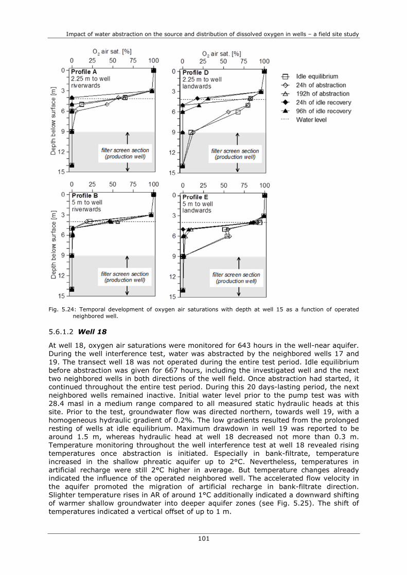
Impact of water abstraction on the source and distribution of dissolved oxygen in wells – a field site study
101
Fig. 5.24: Temporal development of oxygen air saturations with depth at well 15 as a function of operated neighbored well.
Well 18 5.6.1.2
At well 18, oxygen air saturations were monitored for 643 hours in the well-near aquifer. During the well interference test, water was abstracted by the neighbored wells 17 and 19. The transect well 18 was not operated during the entire test period. Idle equilibrium before abstraction was given for 667 hours, including the investigated well and the next two neighbored wells in both directions of the well field. Once abstraction had started, it continued throughout the entire test period. During this 20 days-lasting period, the next neighbored wells remained inactive. Initial water level prior to the pump test was with 28.4 masl in a medium range compared to all measured static hydraulic heads at this site. Prior to the test, groundwater flow was directed northern, towards well 19, with a homogeneous hydraulic gradient of 0.2%. The low gradients resulted from the prolonged resting of wells at idle equilibrium. Maximum drawdown in well 19 was reported to be around 1.5 m, whereas hydraulic head at well 18 decreased not more than 0.3 m. Temperature monitoring throughout the well interference test at well 18 revealed rising temperatures once abstraction is initiated. Especially in bank-filtrate, temperature increased in the shallow phreatic aquifer up to 2°C. Nevertheless, temperatures in artificial recharge were still 2°C higher in average. But temperature changes already indicated the influence of the operated neighbored well. The accelerated flow velocity in the aquifer promoted the migration of artificial recharge in bank-filtrate direction. Slighter temperature rises in AR of around 1°C additionally indicated a downward shifting of warmer shallow groundwater into deeper aquifer zones (see Fig. 5.25). The shift of temperatures indicated a vertical offset of up to 1 m.

Chapter 5
102
Fig. 5.25: Temporal development of hydraulic heads and groundwater temperatures in BF (profile I) and AR (profile H) during well interference test at well 22.
Fig. 5.26: Temporal development of oxygen air saturations with depth at well 22 as a function of operated neighbored well.
Idle equilibrium
At idle equilibrium, the vadose zone was saturated with oxygen in atmospheric concentrations (Fig. 5.26). In the capillary fringe, oxygen air saturations were already significantly lower. At the intersection of vadose and phreatic zone, oxygen was absent in the aquifer. Below the water table, anoxic conditions prevailed in artificial recharge and in bank-filtrate.
Abstraction
As consequence of water abstraction, oxygen entered the cone of depression. This appearance was related with a slight descent of the water level and an imbibition of soil air in the dewatered pores. With continuous abstraction, shallow artificial recharge was only minor enriched by oxygen. It took 360 hours until oxygen entered also the phreatic zone of the aquifer. But the oxic zone remained distinctly below the water table. At
0 5 10 15 20 25Time [d]
26
28
30H
ydra
ulic
hea
d[m
a s
l]
10
12
14
16
18
20
Tem
p [°C
]
0 5 10 15 20 25Time [d]
25
13
Sensor location [m a s l]
29
27
-4
Well
Profile IProfile H
Well 19
Well 18
Well 19
Well 18

Impact of water abstraction on the source and distribution of dissolved oxygen in wells – a field site study
103
abstraction equilibrium, oxygen was only detected in the uppermost layer of artificial recharge and far above the well screen.
Well 22 5.6.1.3
At well 22, oxygen air saturations were observed in the well-near aquifer for 453 hours during a pump test. The pump test included water abstraction by wells 20, 21 and 23. The transect well 22 was not operated during the entire test period. Prior to pumping, all involved wells were resting for 345 hours. Except well 23, who abstracted water for 24 hours three days before the proper pump test. At the beginning of the abstraction period abstraction was initiated at wells 21 and 23 simultaneously. Well 21 was abstracting during the entire test, in contrast, abstraction by well 23 was interrupted after 312 hours. Well 20, located in greater distance, started water abstraction after 240 hours and proceeded until the end of the observation period. Hydraulic heads of the four involved wells were recorded constantly during the investigated period. Initial head at well 22 was with 31.6 masl high, compared to the initial heads observed at other test phases. Both, hydraulic heads at well 21 and well 23 were below those at well 22. The resulting mean hydraulic gradient towards well 23 was with 1% about one magnitude higher than the mean hydraulic gradient to well 21 (0.1%). The maximum observed drawdown in well 22 is 0.8 m, whereas the drawdowns in operated wells 21 and 23 were around 3 m. In well 20, the hydraulic head had dropped only around 2.2 m. Shutdown of well 23 resulted in a recovery of the hydraulic head in well 23 about 2.3 m and in well 22 about 0.3 m within the first 30 hours of idle recovery (see Fig. 5.27).
Fig. 5.27: Hydraulic head developments during well interference test at well 22. (NW=neighbored well)
Idle equilibrium
The temporal development of oxygen air saturations with depth is shown in Fig. 5.28. Initial conditions in the aquifer at idle equilibrium were characterized by atmospheric oxygen saturations in the vadose zone, followed by a transition zone from oxic to anoxic conditions in the upper phreatic aquifer. This transition zone is considerable thinner in groundwater, than in bank-filtrate. But bank-filtrate showed a distinct sequence of anoxic water lying above oxic water, as also observed during previous tests.
Abstraction
Once, abstraction by wells 21 and 23 had started, oxygen distribution in the aquifer at well 22 had changed significantly. Within the first 24 hours of abstraction oxygen air saturation increased in bank-filtrate and groundwater. At the same time the previously observed oxic/anoxic layering obviously persisted in both, groundwater and bank-filtrate. The atmospheric zone in bank-filtrate and groundwater was extended during abstraction
-96 -48 0 48 96 144 192 240 288 336 384Time [h]
27
28
29
30
31
32
Hydra
ulic
hea
d [m
above s
ea le
vel]
Well 22
NW 20
NW 21
NW 23

Chapter 5
104
equilibrium to the water table oscillation zone, including the upper 2 m of the phreatic zone.
The additional operation of well 20, starting after 244 hours, obviously did not affect the oxygen distribution during initial abstraction. But at abstraction equilibrium, the change of flow pattern in the aquifer, provoked by the drawdown in well 20, caused a shift of oxygen air saturation in groundwater. Oxygen increased significantly in the deeper aquifer zone, where it was already present in bank-filtrate. However, the general oxygen distribution pattern did not change by the additional water abstraction at well 20.
Idle recovery
After 312 hours, abstraction at well 23 ended. This in turn, results in an oxygen depletion of the deep GW, which was oxygen-enriched by the previous operation of well 20. As consequence, the oxic zone was shifted upwards in groundwater. Oxygen air saturations in bank-filtrate remained almost unaffected, but showed a slight increase close to the screened aquifer section. Atmospheric oxygen saturations were observed in the vadose zone and in shallow groundwater and bank-filtrate.
Fig. 5.28: Temporal development of oxygen air saturations with depth at well 22 as a function of operated neighbored well.
Conclusions 5.6.2
Investigations of selected well sites revealed an interaction of neighbored wells concerning the distribution and migration of oxic zones (Fig. 5.29). When wells are located closely spaced (<100m), switching of the pumps causes significant changes in the flow field, also of nearby wells. By intermittent operation of adjacent wells, oxic zones resulting from air entrapment and dissolution are forced to migrate following the hydraulic gradient through the aquifer towards neighbour wells. On the flow path, oxygen may be consumed hydro-chemically or biologically at the front of the zone. In the back, the oxygenated aquifer is re-reduced by anoxic, iron-containing water. The migration of oxic, shallow groundwater in the aquifer will further lead to shift of oxygen into deeper aquifer zones. Thus, if wells located closely spaced, the abstraction of oxygenated
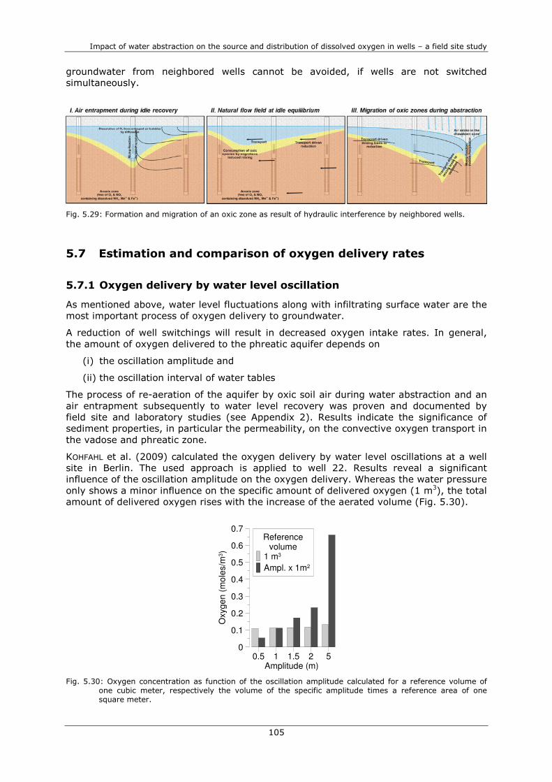
Impact of water abstraction on the source and distribution of dissolved oxygen in wells – a field site study
105
groundwater from neighbored wells cannot be avoided, if wells are not switched simultaneously.
Fig. 5.29: Formation and migration of an oxic zone as result of hydraulic interference by neighbored wells.
Estimation and comparison of oxygen delivery rates 5.7
Oxygen delivery by water level oscillation 5.7.1
As mentioned above, water level fluctuations along with infiltrating surface water are the most important process of oxygen delivery to groundwater.
A reduction of well switchings will result in decreased oxygen intake rates. In general, the amount of oxygen delivered to the phreatic aquifer depends on
(i) the oscillation amplitude and
(ii) the oscillation interval of water tables
The process of re-aeration of the aquifer by oxic soil air during water abstraction and an air entrapment subsequently to water level recovery was proven and documented by field site and laboratory studies (see Appendix 2). Results indicate the significance of sediment properties, in particular the permeability, on the convective oxygen transport in the vadose and phreatic zone.
KOHFAHL et al. (2009) calculated the oxygen delivery by water level oscillations at a well site in Berlin. The used approach is applied to well 22. Results reveal a significant influence of the oscillation amplitude on the oxygen delivery. Whereas the water pressure only shows a minor influence on the specific amount of delivered oxygen (1 m3), the total amount of delivered oxygen rises with the increase of the aerated volume (Fig. 5.30).
Fig. 5.30: Oxygen concentration as function of the oscillation amplitude calculated for a reference volume of one cubic meter, respectively the volume of the specific amplitude times a reference area of one square meter.
0.5 1 1.5 2 5Amplitude (m)
0
0.1
0.2
0.3
0.4
0.5
0.6
0.7
Oxyge
n (
mo
les/m
3)
Referencevolume
1 m3
Ampl. x 1m2
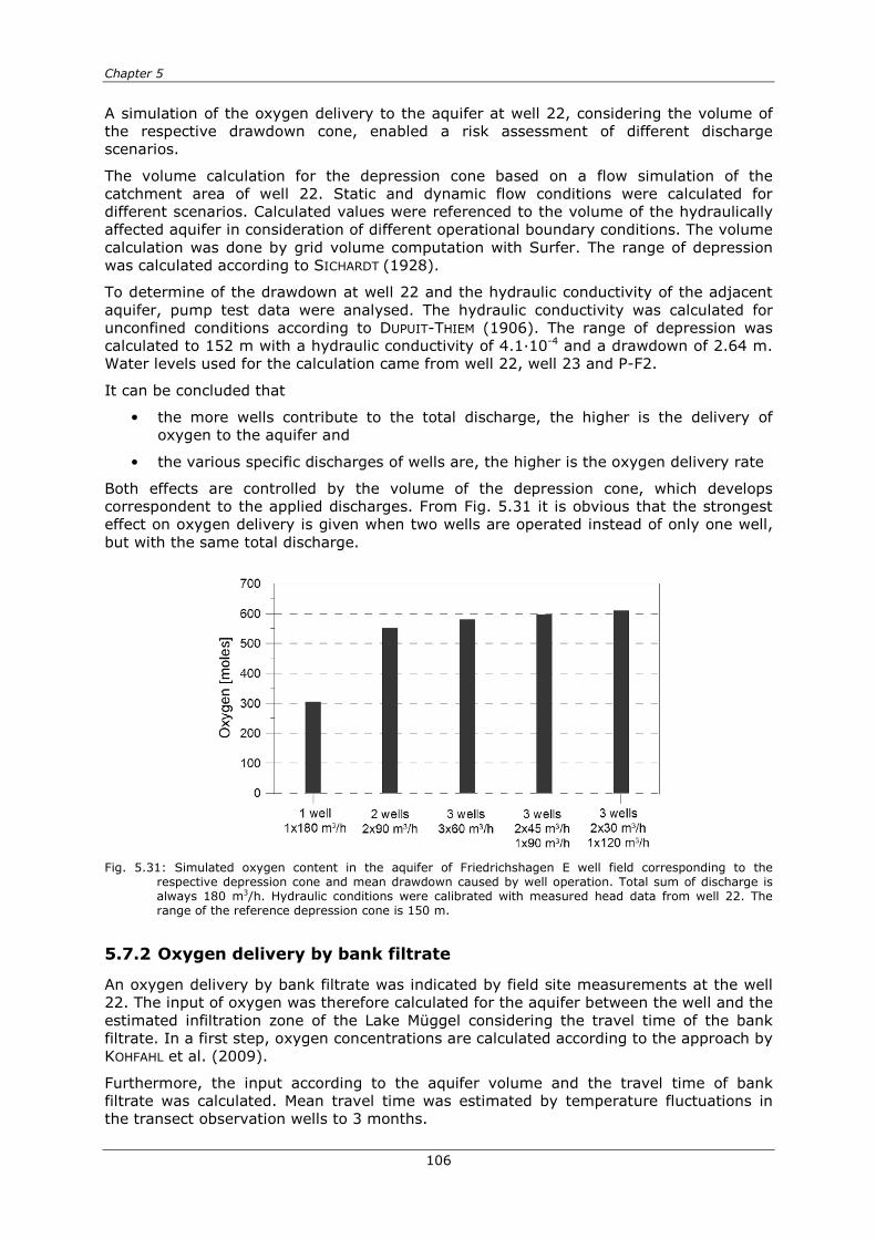
Chapter 5
106
A simulation of the oxygen delivery to the aquifer at well 22, considering the volume of the respective drawdown cone, enabled a risk assessment of different discharge scenarios.
The volume calculation for the depression cone based on a flow simulation of the catchment area of well 22. Static and dynamic flow conditions were calculated for different scenarios. Calculated values were referenced to the volume of the hydraulically affected aquifer in consideration of different operational boundary conditions. The volume calculation was done by grid volume computation with Surfer. The range of depression was calculated according to SICHARDT (1928).
To determine of the drawdown at well 22 and the hydraulic conductivity of the adjacent aquifer, pump test data were analysed. The hydraulic conductivity was calculated for unconfined conditions according to DUPUIT-THIEM (1906). The range of depression was calculated to 152 m with a hydraulic conductivity of 4.1·10-4 and a drawdown of 2.64 m. Water levels used for the calculation came from well 22, well 23 and P-F2.
It can be concluded that
• the more wells contribute to the total discharge, the higher is the delivery of oxygen to the aquifer and
• the various specific discharges of wells are, the higher is the oxygen delivery rate
Both effects are controlled by the volume of the depression cone, which develops correspondent to the applied discharges. From Fig. 5.31 it is obvious that the strongest effect on oxygen delivery is given when two wells are operated instead of only one well, but with the same total discharge.
Fig. 5.31: Simulated oxygen content in the aquifer of Friedrichshagen E well field corresponding to the respective depression cone and mean drawdown caused by well operation. Total sum of discharge is always 180 m3/h. Hydraulic conditions were calibrated with measured head data from well 22. The range of the reference depression cone is 150 m.
Oxygen delivery by bank filtrate 5.7.2
An oxygen delivery by bank filtrate was indicated by field site measurements at the well 22. The input of oxygen was therefore calculated for the aquifer between the well and the estimated infiltration zone of the Lake Müggel considering the travel time of the bank filtrate. In a first step, oxygen concentrations are calculated according to the approach by KOHFAHL et al. (2009).
Furthermore, the input according to the aquifer volume and the travel time of bank filtrate was calculated. Mean travel time was estimated by temperature fluctuations in the transect observation wells to 3 months.

Impact of water abstraction on the source and distribution of dissolved oxygen in wells – a field site study
107
The volume of the aquifer zone oxidized by bank filtrate was calculated corresponding to the width of the infiltration zone, the thickness of the oxic aquifer layer and the distance between the well and the lake.
The oxic zone located in the aquifer between the well and the lake was estimated to be of triangular shape with the greatest thickness close to the well (length=100 m; height=20 m). The total volume of the oxic aquifer zone between the well and the lake was calculated to ~50.000 m3.
Maximum and minimum oxygen concentrations in bank-filtrate of 8 mg/l (max) and 2 mg/l (min) were derived from field site measurements at well 22 at the well screen top. The range of oxygen concentrations in bank filtrate are controlled by the infiltration conditions which are strongly connected with seasons and with the operational state of neighbored wells.
The analytically calculated oxygen delivery to the phreatic aquifer by water level oscillations exceeds the oxygen delivery by bank filtrate by a factor of 2 to 10, dependent on the oxygen concentration in bank filtrate (Fig. 5.32). This distinct dominance of water level oscillations for the oxygen enrichment of anoxic groundwater could not be clearly verified by the field measurements. Oxygen distribution in the well-near aquifer shows a differentiated pattern. Highest concentrations are present in the cone of depression, but oxic bank filtrate seems to be the dominating source of oxygen close to the well screen.
Fig. 5.32: Oxygen concentration calculated for infiltrating oxic surface water in summer (8 mg/l) and winter (2 mg/l) compared to those produced by oscillation of groundwater level.
Based on the results of site studies at well 22, ratio of oxygen delivery by well switching and by bank filtration can be estimated.
In case of well switching as source for oxygen delivery, values were calculated in consideration of the extent of the cone of depression caused by the discharge of the corresponding number of wells. The depression cones were simulated regarding the local flow field and the kf-values. Furthermore, specific travel times for the different discharge scenarios, derived from flow simulations, were considered for the calculation of the oxygen delivery by bank filtrate.
The oxygen delivery to well 22 as result of switching and as result of abstracting bank filtrate is compared and regarded to assess the relevance of both oxygen pathways for redox dynamics in the well. Results are presented in Fig. 5.33. Thus, the oxygen delivery by bank filtrate depends on the discharge and on the number of operating wells, whereas the input of oxygen from well switchings can be minimized by abstracting the same volume of water with more wells but with less specific discharge.
0.5 1 1.5 2 5Amplitude (m)
0
0.05
0.1
0.15
0.2
Oxyge
n [m
ole
s/m
3]
Groundwater
8 2cDO [mg/l]
Bank filtrate

Chapter 5
108
Fig. 5.33: Theoretical ratio of oxygen delivery by well switching and influx by bank filtration, calculated exemplarily for well 22 (share of bank filtrate: ca. 80%). Labels of abscissa describe the scenario, i.e. the number of wells operating and their discharge rate.
Further, the minimum oxygen delivery by bank filtrate is equal to the delivery from two to 23 well switchings per year, depending on the number of wells and the total discharge. The maximum oxygen delivery by bank filtrate is equal to 50 to 175 well switchings per year, respectively.
Implications for well clogging processes 5.8
According to the varying performance data of the three wells, they also vary in the redox condition of their recharge. As described above, oxygen distribution pattern differ significantly between all wells considering the four abstraction phases and the abstraction period. But all wells have in common, that abstraction causes an oxygen enrichment of the well-near aquifer and a downward shift of the oxic/anoxic interface.
The amount of oxygen delivered to groundwater and the offset of the interface in the aquifer vary between the well sites. Differences are also observed in the performance development of the wells. Well 15 has lost only 20% of his initial well yield and existing clogging deposits are mainly limited to a preferred direction from the top of the screen downwards. This is only minor reflected by a screen loss of 0.04 m. Abstracting groundwater from an aquifer, with a shallow oxic/anoxic interface as observed at well 15, lead to a mixing of the shallow oxic with the deep anoxic water close to the well (VAN
BEEK et al. 2009), and to increased incrustations at the top of the screen (RIEMPP 1964, HOUBEN & TRESKATIS 2007). Once the upper screen is clogged, clogging will move gradually downwards (HOUBEN & TRESKATIS 2007, VAN BEEK et al. 2009).
Based on the relatively homogeneous oxygen distribution in the well-near aquifer at well 15 in groundwater and bank filtrate direction, a more homogeneous distribution of deposits in the well is assumed. But the anisotropic incrustations are also reflected by a low well screen loss, which only represents the loss in the direction, the filter pack piezometer is oriented. According to HOUBEN and TRESKATIS (2007), an inhomogeneous distribution of incrustations reflects the flow field superimposed by the well onto the natural groundwater regime. In that case, incrustations are stronger in groundwater direction. The presence of shallow oxic groundwater and the downward shift of the oxic/anoxic interface during abstraction results in the contribution of oxic water to the well. The fact, that abstracted well water is free of dissolved oxygen indicates a degradation of the dissolved oxygen near to and in the well. Due to the presence of

Impact of water abstraction on the source and distribution of dissolved oxygen in wells – a field site study
109
dissolved iron(II) in the anoxic deeper groundwater a precipitation of iron(III)hydroxides is possible, when dissolved iron is oxidized. The mixing of oxic and anoxic groundwater near to the well can be strongly enhanced by large values of transversal dispersion (VAN
BEEK et al. 2009). Further, the gradually proceeding of incrustations clogging the slots downward from the top of the screen may result in decreased rates of shallow oxic groundwater to the total abstracted water (VAN BEEK et al. 2009). Thus, clogging already takes place in the gravel pack and the nearby aquifer. The occurrence of strong incrustations in the well-near aquifer was identified as result of abstracting water by a well for decades (HOUBEN & WEIHE 2010). VAN BEEK (2010) argue that the short residence times are not favourable for an extensive deposition of incrustations. He follows, that the main phase of ochre formation is during water level recovery, when increased permeabilities in well and filter pack lead to a mixing of waters with different redox states as they were filling up the cone of depression (VAN BEEK 2010). But the degradation of dissolved oxygen along the flow paths towards the well screen clearly indicate the oxidation of dissolved iron in the aquifer and the filter pack during abstraction. The iron deposits inside well 15 are obviously dominated by biological structures. Iron-oxidizing bacteria prefer high flow velocities, because a constant supply of required nutrients (dissolved iron(II) and oxygen) is well provided (KREMS 1972, CULLIMORE 1999, HOUBEN & TRESKATIS 2007). This applies particularly for the screen slots of well and pump, but also in the upper well zone and in the filter pack at and above the screen top. The fast degradation of oxygen observed at well 15 during water level recovery also point to oxidation processes within the aquifer. In consideration of the oxygen distribution and development, well 15 owns a high clogging potential. Apparently, this conclusion is inconsistent with the real, observed clogging rate. But the decisive factor, controlling the performance loss of well 15 is the influx distribution at the well. In contrast to most other wells, where influx is greatest at the screen top (HOUBEN 2006), main influx at well 15 is in the lower screen section.
At both other wells, influx is mainly provided by the upper screen section, the one to two most upper meters in particular. The observed oxygen distribution in the aquifer close to well 18 indicates a less significant delivery of oxygen by fluctuating water tables, since even the shallow groundwater is anoxic. Correspondingly, screen loss is minor. But the loss in performance is huge (40%), considering the age of the well (3 years). Because well 18 abstracted predominantly groundwater and “old” bank filtrate during the sampling period, observed oxygen distribution is only a snap-shot and does not represent neither seasonal variations nor the filling cycle of the recharge pond. Both effects significantly affect the aeration status of the aquifer (GRESKOWIAK et al. 2005). Thus, it can be assumed, that clogging rates vary correspondingly to the aeration status of the aquifer. Comparatively low iron(II) and high nitrate concentrations, combined with a relatively high redox potential in the abstracted well water may express the presence of suboxic conditions in the aquifer. Oxidation of dissolved ferrous iron by nitrate-reducing microorganisms in the suboxic zone may also contribute considerably to the formation of iron incrustations (EHRENREICH & WIDDEL 1994, STRAUB et al. 1996).
Well 22, with the lowest initial well yield of the three wells, shows also extensive clogging rates, indicated by a significant loss in performance (35%) in spite of lately realized rehabilitation measures. The comparatively high screen loss of 0.45 m is also illustrated by the presence of a substantial amount of incrustations at the top of the screen. Additional to the heterogeneous vertical distribution, deposits show a clear anisotropic character. Deposits are located predominantly at the side directed towards the lake and with less intensity towards neighbored wells. In groundwater direction, incrustations are almost absent. Oxygen measurements in the well-near aquifer reveal a combined intake of oxygen into the groundwater by fluctuating water tables and oxic bank filtrate. The deposit distribution in the well thus correlates distinctly with the oxygen distribution in the aquifer. The high variability of oxygen air saturation during abstraction and recovery in groundwater direction indicates a mixing of oxic bank filtrate with anoxic groundwater already in the aquifer, resulting in oxidation of dissolved ferrous iron. Because surface water infiltrates at the lake banks and through the slightly declining lake bed, the oxic

Chapter 5
110
zone is limited to the upper aquifer near the lake. By transversal dispersion (VAN BEEK et al. 2009) and fluctuating water tables (WILLIAMS & OOSTROM 2000) due to intermittent well operation, the oxic zone is widening towards the abstracting well (MASSMANN et al. 2008). The observation, that bank filtration wells show incrustations at deeper well sections, because water mainly infiltrates at lake beds (HOUBEN & TRESKATIS 2007), does not apply to Berlin bank-filtration well sites. Due to the impermeable beds of Berlin lakes, infiltration takes place in the narrow zones at the shores, resulting in a vertical age stratification of bank-filtrate getting progressively older with depth (MASSMANN et al. 2008). Hence, the influence of oxic bank filtrate on the clogging potential cannot necessarily be identified based on the incrustation distribution in the well.
Conclusions 5.9
Based on an in-situ monitoring of oxygen in the well-near aquifer of three Berlin well sites, abstracting groundwater from aquifers with different recharge sources (bank filtrate, groundwater, AR), the impacts of the different water abstraction phases on the oxygen distribution were identified.
The used monitoring network composed of multi-level observation wells and vertical optode strings installed in aquifer and inside the wells was feasible to measure changes in hydraulic conditions and redox dynamics with regard to oxygen. Oxygen distribution could be observed as a function of depth, recharge source and time in a high resolution for the first time. Thus, it was possible to detect traces of oxygen in the well-near aquifer and inside the wells, which are sufficiently to oxidize high loads of dissolved iron when supplied constantly.
Measurements revealed that during the initial abstraction phase, the oxic zone and the oxic/anoxic interface present in groundwater prior to abstraction are significantly shifted downwards at all well sites. Partially, highly variable oxygen saturations in this phase indicate the oxidation of ferrous iron as anoxic iron(II)-containing and oxic water mixes in the well-near aquifer. Thus, during the initial abstraction phase, precipitation of iron(III)hydroxides occurs mainly in the aquifer.
Flocculated iron(III)hydroxides then may be transported along the flow paths to the well, but are also able to clog sediment pores. Once abstraction equilibrium is reached, oxygen saturations close to the well stabilize. In this phase, clogging of screen slots by biological oxidation dominates. This is suggested by the absence of dissolved oxygen in the groundwater as it enters the well and by the high bio mass portions in incrustations.
Once abstraction ends, dissolved oxygen is depleted within hours as a result of a replacement of oxic water by a vertical ascent and a horizontal influx of anoxic water refilling the cone of depression. In zones, with higher permeabilities, like filter pack and well, a mixing of anoxic and oxic water may occur in the case that the oxic/anoxic interface is located below the screen top. This behavior was not observed at the three Berlin well sites. But primarily, the presence of oxic bank-filtrate in the well-near aquifer of a Berlin bank-filtration well site could be observed.
Until now, oxic conditions were only encountered in bank-filtrate close to the banks in winter and in shallow groundwater close to the wells. The infiltration of oxic bank-filtrate or artificial recharge delivers high amounts of oxygen to the groundwater and can cause an enormous widening of the oxic zone towards the abstracting well. As a result, the oxic/anoxic interface turns upward close to the well once water is abstracted. Further, clogging of wells abstracting bank filtrate or artificial recharge strongly depends on the residence times of the filtrate, the hydraulic connection between banks and groundwater and seasonal variations. Only under certain conditions a significant enhancement of clogging can be expected.

Impact of water abstraction on the source and distribution of dissolved oxygen in wells – a field site study
111
To clearly determine the impact of these factors, a monitoring of the oxygen distribution throughout the seasons would be necessary. Additional to the determination of oxygen input rates, depth oriented hydro-chemical sampling including redox sensitive parameter as dissolved ferrous iron, dissolved manganese and nitrate would provide the data for a site specific modelling of precipitation rates and their impact on well performance. On the basis of this research an adopted well operation scheme can be implemented to reduce the input of oxygen into the aquifer and to prevent intense clogging and high performance losses of wells in future. An estimation of the clogging potential of wells would imply their classification according to their hydraulic behavior, their recharge conditions, their constructional characteristics, including the intake zones, and their position in the well field. This classification could also serve as basis for the planning and application of prevention and rehabilitation measures.


Oxygen dependency of iron related clogging processes
113
Chapter 6
Oxygen dependency of iron-related
well clogging processes – a hydraulic,
hydrochemical and geochemical well
model study
Introduction 6.1
The supply by reactants and nutrients is fundamental for the formation of ochre deposits in wells. The ample presence of reactants and nutrients needed for biochemical iron oxidation processes, provided e.g. by high flow rates, enables a development of appreciable ochre deposits (CULLIMORE 1999). Dissolved oxygen and iron are the main reactants for the biochemical precipitation of oxidized iron species (VAN BEEK 2010). Oxygen is mainly delivered to the groundwater by frequent water table fluctuations (KOHFAHL et al. 2009). The stronger the water table oscillations the higher the amount of oxygen in shallow groundwater. This process is reflected by a vertical hydro-chemical zonation in aquifers, with increasing thickness of the oxic groundwater layer in the vicinity of wells (MASSMANN et al. 2006b).
Thus, both reactants, dissolved oxygen and Fe(II), do not exist simultaneously in native groundwater. They primarily mix when they were both forced to enter the well at the top of the screen at the same time. As result, ochre formation takes place and decreases porosity and permeability of the affected area, causing a change of inflow pattern and a loss of well performance.
The flow field in the vicinity of wells is therefore another driving factor for ochre formation. The distribution of flow velocities in the vicinity of a well is depending on vertical inhomogeneities of the aquifer and on the geometry of the well. All water which overlies the well screen enters the well at the top of the screen. Therefore, flow velocities are highest in the upper screen section. From model simulations, it is known that the upper third of the screen can provide almost 50 % of the total water inflow (HOUBEN 2006). But the true inflow distribution at a well can only be assessed by performing flow meter inside the well. The relevance of ochre formation for a change in well performance is strongly related to the inflow distribution. Wells which are mainly supplied by the most upper part of the well screen are rather responsive to well yield losses than wells which are supplied evenly over the whole well screen. The inflow distribution can vary strongly within the same well field, although hydrogeological conditions seem to be homogenous for all wells. As a result, one well shows strong performance losses, whereas his neighbour well almost kept his performance.
Well performance can be assessed and monitored by the development of the discharge rate-drawdown ratio, but information about variations in porosity and permeability in aquifer and filter pack are lacking. Therefore, it is not possible to directly link the degree of ochre formation to the loss of well performance. Deposit samples are at least available when wells are reconstructed. Further, the availability of undisturbed sediment or filter pack samples is strongly limited due to technical limitations. The development of a sampling device for horizontally core sampling was planned within the WELLMA project, but yet not accomplished.

Chapter 6
114
Correlation of hydraulic, hydro-chemical and geochemical conditions is needed to estimate and calculate their impacts on well ageing rates as result of iron-related clogging processes. Information about the clogging process and especially the clogging rate at the passage from aquifer to filter pack to well screen are strongly limited. WEIDNER et al. (2012) reproduced the chemical formation of Fe-hydroxide incrustations in an experimental model under controlled boundary conditions. A clogging of the gravel material was quantified by measuring the hydraulic head in the filter pack. The hydraulic gradient increases up to 75 %. In a second model run 15g Fe/kg gravel were produced and correlated with a pressure loss of 30% in the filter pack (HENKEL et al. 2012). Because of the complex bio-chemical process of iron precipitation and biofilm formation under suboxic conditions, a study of clogging rates is unrewarding, if it is realized in an artificial experiment setup excluding biological processes.
To link analytically calculated as well as chemically analysed iron precipitation rates with monitored well performance data and oxygen availability, a tank with a model well was developed and constructed. The model well should provide the possibility to relate the input and distribution of dissolved oxygen to a temporal decrease in specific well yield and to a temporal decrease in the permeability of sediment and filter pack. Therefore, it was essential to build a tank, where hydrogeological conditions are close as possible to those of a real well. Therefore, the model well was run with native groundwater. Based on data characterising the flow field and the redox state within the tank and combined with in- and output rates, a balancing and calculation of precipitation rates should be feasible.
Furthermore, the study concept should admit the determination of well deterioration with regard to the operation scheme of the well. Impacts of varying switching intervals and different pumping rates should be able to assess.
Methods 6.2
Model well design 6.2.1
To provide the transferability of results to a real well, dimensions, used materials and sediments for the construction and filling of the model well were chosen corresponding to a typically drinking water well of the Berliner Wasserbetriebe with a borehole diameter of 900 mm and a casing diameter of 400 mm (in a scale 1:1). Thus, the model well includes a wire-wound stainless steel (Johnson screen) and a stainless steel casing, a twofold filter pack and original aquifer sediment (Fig. 6.1 left).
The tank used as model well is made of stainless steel elements, which shape an equilateral triangle with an angle of 30° (Fig. 6.1 right). Because of its triangular shape, the tank provides a radial flow towards the well. This is relevant in order to consider the increasing flow velocities towards a well.
To prevent a direct aeration of the well screen, the dynamic water level in the well should be always above the top of the screen during the experiment run. Initially, the screen was set to a length of 65 cm. After a short calibration phase in the laboratory, the screen was shortened to 50 cm length, by taking into account, that drawdown increases as clogging proceeds during the experiment.
The twofold filter pack consists of an inner part filled with gravel and an outer part filled with sand. Both were aligned to the aquifer material and were covered by a sealing clay layer. Material properties are given by Tab. 6.1.
The bulk material used for the aquifer originates from a well drilling at a bank filtration site in Berlin-Schildhorn. The matching for a correct filter pack dimensioning was done according to the dimensioning of the filter pack for the new constructed drinking water well in Berlin-Schildhorn.

Oxygen dependency of iron related clogging processes
115
The aquifer compartment is separated by a stainless steel fine-meshed screen from the influx distributor. The influx distributor is vertically segmented into five chambers. This enables an influx control by water valves installed at each chamber (see also App. 8). Additionally to the water inlet, each chamber has a water outlet with a defined pressure head. The pressure head is given by a static overflow level, which corresponds to the top of the tank. The constant pressure heads provide a homogeneous pressure distribution in all five chambers.
Fig. 6.1: Upper Left: Schematic illustration of the radial flow towards the well in the constructed tank. Upper Right: Modular setup of the model well with different compartments for the well (I), the inner (II) and outer filter pack (III), the aquifer (IV) and the influx distributor (V). Lower Left: Tank installation at field site. Lower right: well model compartments with the different filling materials.
Tab. 6.1: Soil type, unconformity and hydraulic conductivity (after BEYER) of the different filling units of the well tank.
Unit Grain size Uniformity Hydraulic conductivity
[m/s] Porosity
[%] neff
[%]
Aquifer sediment mS, fs 2,9 4.2*10-4 30.6 -
Filter sand 0,7 - 1,8 mm 1,5 5.0*10-3 43.3 33
Filter gravel 2 - 8 mm 1,4 2.8*10-1 24.1 24

Chapter 6
116
Monitoring design 6.2.2
The monitoring includes hydraulic heads and parameter controlling the hydro-chemical formation of iron precipitates. Changes in the hydraulic behaviour were observed using piezometers and tracer tests in combination with a metering of discharge rates. An online monitoring of oxygen was done by oxygen-sensitive probes (optodes) and a hydro-chemical sampling and analysis assessed the water quality at the in- and outflow. Furthermore, ochre deposits were sampled after the experiment run. Monitoring and sampling activities are summarized in Tab. 6.2 and specified below.
Tab. 6.2: Type and no. of sampling at the model well.
Subject Sample location No. of samples/measurements
Hydrochemistry
Inflow Complete 5
Fe, Mn 19
Outflow Complete 6
Fe, Mn 31
Oxygen Optodes 8
Hydraulic heads Piezometer 39
Tracer test Pump 16
Deposits
Aquifer sediment 13
Filter sand 8
Filter gravel 12
Installation 2
The discharge rate was determined using a calibrated customary water meter. The rate was read frequently to control in- and outflow of the well model and event based analogous to measurements of the hydraulic heads in order to calculate specific well yield.
The monitoring network for the assessment of the hydraulic heads consists of 44 observation tubes (piezometer). The monitoring of hydraulic heads was done event-based, regarding the operational status of the tank. Piezometers were primarily placed at the interfaces of the different tank units. Here, changes in permeability and porosity are expected to be greatest. For the detailed locations of the piezometers see App. 8.
The monitoring network for oxygen measurement consisted of 22 oxygen-sensitive probes (optodes). The monitoring of oxygen was done event-based, regarding the operational status of the tank and the respective hydraulic heads. Before installation, the optodes were two-point calibrated at 0 and 100% oxygen air saturation. The oxygen probes were placed in the aquifer and the filter pack unit, aligned with the piezometer and closer meshed towards the well. For the detailed locations of the optodes see App. 8.
Tracer tests were performed event-based to calculate the effective porosity change with time. Sodium-chloride was used as tracer and detected with an electrical conductivity meter. It turned out in the calibration phase, that 500 ml solution with a sodium-chloride concentration of 4 g/L was the most suited relation. The tracer was inserted in the aquifer unit directly behind the fine-meshed screen, separating the influx distributor from the aquifer material, and was detected at the outflow of the submersible pump.
The hydro-chemical composition of the inflowing water at the inlet of the well tank, as well as the outflowing water behind the pump, was analyzed event-based. In- and outflow were sampled constantly for Fe and Mn species. The inflow was sampled 14 times, the outflow 25 times. Extended hydro-chemical analysis was done 5 times in a greater interval including T, pH, Eh, EC, NH4, Fe, Mn, NO3, NO2, PO4 and main ions.
The sampling of ochre deposits was done at the end of the experiment run. 33 disturbed deposit samples were taken from the different well model units. All samples were analysed for their Fe and Mn-content. In addition to the bulk material samples, two ochre

Oxygen dependency of iron related clogging processes
117
samples were collected from the submersible pump and the riser pipe. The precipitates were solubilized and separated from the sediments by cooking with aqua regia. Afterwards the solutes were diluted with purified water to 100 ml and analysed by a photometer. A list of all samples is shown in App. 9.
Experiment design 6.2.3
The model well was operated with abstracted well water in order to ensure natural thermodynamic and microbiological conditions as they are present in the aquifer. Therefore, the model well was installed at a drinking water well site to provide a constant water supply.
The abstracted water had to meet specific requirements. Because ochre formation and clogging should occur in the model well and not already before in the drinking water well, the well had not to tend to enhanced iron related clogging. Thus, the selected well had to be located in a confined aquifer, where oxygen is not or only in minor extent able to enter groundwater through the vadose zone. To minimize oxidation processes in the abstracted water, oxidative species, such as O2 and NO3 had almost to be absent in the water. Further, the well had to be operated continuously to provide a constant supply of the model well. For safety reasons, the well had to be situated in a fenced water work area.
All these criteria apply to a well which is part of a well field belonging to the water work Spandau (Tegel).
The hydro-chemical composition and condition of the abstracted water is shown in Fig. 6.2. PH and redox potential were moderate with 7.4, respectively 140 mV. Fe(II) had a median concentration of 1.4 mg/l, O2 was absent and NO3 was only present in low concentrations of about 0.1 mg/l and below.
Fig. 6.2: Box-plots of significant hydro-chemical parameter of the selected well.
The main goal of the model well experiments was the in-situ oxidation of Fe(II) and the formation of ochre deposits as result of an aquifer aeration by air entrapment. Ochre formation and clogging of wells is an on-going process, which takes months to years to be obvious and of relevant extent. To take this into account, the experiment run for a period of 390 days. It was expected, that, if oxidative processes were accelerated by
500
600
700
800
900
1000
EC [µS/cm]
7
7.1
7.2
7.3
7.4
7.5
7.6
pH
100
120
140
160
180
Eh [mV]
0.12
0.13
0.14
0.15
NH4 [mg/l]
1.3
1.4
1.5
1.6
1.7
Fe [mg/l]
0.3
0.32
0.34
0.36
0.38
0.4
Mn [mg/l]
0
0.01
0.02
0.03
NO2 [mg/l]
0.09
0.1
0.11
NO3 [mg/l]
0.1
0.2
0.3
0.4
0.5
PO4 [mg/l]
n=6
n=6
n=3n=3
n=4
n=4
n=3
n=3n=4

Chapter 6
118
frequent water table oscillations, within this timescale significant amounts of Fe(II) could be oxidized to Fe(III) and deposited at filter pack materials and installations.
The experiment run had three different operation phases concerning the flow conditions in the model well: 1. Constant flow phase, 2. Stagnant flow phase and 3. Transient flow phase. The operational data characterising the different experiment phases are summarized in Tab. 6.3.
In the first experiment phase, the model well was operated under constant flow
conditions for a period of 22 days. During this period, the abstracted anoxic water should establish reduced conditions in the model well by filling up and flowing through the tank. Because sediments were kept sealed in barrels and were deposited in the well model under water saturated conditions, they were almost not oxidized. In addition, this period was used as reference for later occurring changes in hydraulic and hydro-chemical conditions. For such a calibration of the model well, baseline monitoring of hydraulic heads, oxygen and Fe-species under unaffected conditions was mandatory.
In the second experiment phase, the model well was resting under stagnant flow
conditions for a period of 11 days. During this period, oxygen was monitored to identify a potential oxidation of the anoxic model well by diffusive processes. Basing on the results, the diffusive component on the aeration of the model well was determined.
The third experiment phase included alternating sequences of operation and recovery periods. The model well was operated with transient flow conditions for about 255 days. Within the first 157 days, operation was intermitted specifically for 36 times with resting periods between 3 to 48 hours. This operation scheme simulated the operational mode of a drinking water well. After that period, the model well was resting due to a supply interruption under stagnant flow conditions for a period of 87 days. During the remaining 98 days, operation of the model well was intermitted for 208 times with resting periods between 2 to 4 hours. This operation scheme should accelerate the Fe(III)-precipitation rates to the most possible extent.
Tab. 6.3: Summary of the operational conditions during the three phases of the model well experiment run.
Scheme of experiment phase Duration Mean pumping rate Pumped volume Number of
swichtings days m3/h m3
1 constant flow 22 0.16 85.54 0
2 stagnant flow - - - -
3 transient
flow
3 hours operation - 48 hours recovery
244 0.10 79.3 36
6 hours operation - 2 hours recovery
98 0.06 46.5 208
Total 390 0.11 211.3 244
Results and discussion 6.3
Constant flow conditions 6.3.1
The hydro-chemical composition was strongly affected during the model well passage under constant flow conditions. While the main ion composition was stable, redox sensitive parameter showed relevant differences between in- and outflux. Fe(II), NH4 and NO3 were present in higher concentrations in the influx compared to the outflux. Fe(II) was reduced by a factor of 0.35 from 1.7 to only 0.6 mg/l during passage. Fe(III) was not present in in – and outflux in significant concentrations. Fe(II) concentrations almost corresponded with Fe(total) concentrations in all samples. NH4 and NO3 were both reduced by a factor of 0.6. O2 was slightly enriched from 0.00 mg/l in influx to 0.02 mg/l in outflux. PH was lowered from 7.37 to 7.29 and the redox potential increased from 25 to 100 mV. Both, the increase of H+ and the increase of redox potential indicated the

Oxygen dependency of iron related clogging processes
119
oxidation of Fe(II) to Fe(III). Only Mn(II) underwent no significant change during the passage.
Thus, oxidation of Fe(II) to Fe(III) and precipitation as Fe(OH)3 already took place under constant flow conditions, where the delivery of O2 was strongly limited. All measurements of O2 concentrations revealed that anoxic conditions dominated in the water saturated zones of the model well. During constant flow conditions O2 was only detected in soil air. Below the water table, O2 was not traceable. As long as the model well run under constant flow conditions no O2 delivery from soil air to groundwater was observed. The only present process of O2 enrichment in groundwater, diffusion, obviously had no relevant impact on the spatial distribution of O2 in the well model.
In general, the flow field within the model well was characterized by a horizontal flow below the screen top. Above the screen top the vertical flow component increased in flow direction towards the well. In the filter pack, above the screen top, flow was nearly vertically. Thus, the observed flow field corresponded to the theoretical and simulated flow fields, as they are assumed at real well sites (HOUBEN 2006).
The specific yield of the model well was in the range of 0.028 m3/h/m, the effective
porosity was calculated basing in the tracer tests to 53%. Because porosities of filter and aquifer material were determined to less than 43%, the effective porosity values were not in a plausible range. This deviation was presumably caused by the substantial differences in hydraulic behaviour of the different bulk material used in the model well. Thus, effective porosity had to be taken as relative parameter, where only the changes could be considered.
Stagnant flow conditions 6.3.2
Within the first 11 days of stagnant flow conditions no O2 delivery was traceable in the model well. O2 was not detected below the water table, but in the vadose zone with concentrations below atmospheric air saturation.
During the second period of stagnant flow conditions, between the two transient flow periods, O2-distibution was similar to the distribution during the first stagnant period. The diffusive delivery of O2 was neglectable. But as shown in Fig. 6.7, specific well yield as well as effective porosity seemed to be rehabilitated during the extended period of stagnant flow conditions. It was conceivable, that under stagnant flow conditions redox processes favoured the re-dissolution of Fe(III). This was already be observed for Fe(III) in biofilms, when redox conditions changed from oxidizing to reducing (THRONICKER & SZEWZYK 2011). But the role of iron-oxidizing and –reducing bacteria for the ochre formation in the model well was not further considered by this study.
Transient flow conditions 6.3.3
Transient flow conditions were established by an intermittent model well operation. The hydro-chemical composition of in- and outflux varied significantly for redox sensitive parameter. Hydro-chemical analysis of in- and outflux samples are given in Fig. 6.3.
Balancing of Fe(II)-content in in- and outflux pointed out a mean loss of 80% during the model well passage under transient flow conditions. The missing Fe(II) had to be retained in the model well, because Fe(total)-concentrations were at the same level as Fe(II)-concentrations. This supports the assumption, that O2 delivery and therefore Fe(II) oxidation is promoted by an intermittent well operation. Mn(II) was slightly but remarkable reduced during the passage by 3 %, whereas it was unaffected under constant flow conditions. The prolonged oxidation of Mn(II) was reflected by a stronger enrichment with O2 and a stronger increase of the redox potential compared to constant flow conditions. O2 was found enriched in the outflux with up to 0.5 mg/l. The reduction of NH4 under transient flow conditions seemed not to be affected by the stronger oxidative environment and coincided with the reduction under constant flow conditions.

Chapter 6
120
NO3, by contrast, showed no reduction between in- and outflux, although it was reduced during constant flow conditions. If NO3 was reduced by oxidizing Fe(II) to Fe(III) during constant flow conditions, is to debate. But it is a fact that as long as O2 was present in significant amounts in the outflux, NO3 concentrations remained unaffected during the passage.
Fig. 6.3: Box plots of redox sensitive parameter in the in- and outflux of the model well including samples from all three experiment phases.
By the change of Eh-pH-conditions during the model well passage, a chemical precipitation of Fe(II) was indicated as shown by
Fig. 6.4. Redox potential increased strongly from 40 to 130 mV and pH was lowered considerably from 7.47 to 7.38. Considering the specific hydro-chemical composition for the position of stability fields in the Eh-pH-diagram, the increase of redox potential caused a shift from the Fe²+ stability field to the Fe(OH)3 field, while the decreasing pH-value rather counteracted an enhanced FE(II)-oxidation. Indeed, influx water was already close to or even was within the stability field of Fe(OH)3.
Fe(II) concentrations in the outflow showed a broad dependency on the time lag between initiation of pumping and sampling (Fig. 6.5). Subsequent to the start of pumping, Fe(II) concentrations were low but increased with time. This indicated a precipitation of Fe(II) during stagnant or slow flow conditions in the model well. After 2-3 hours the water in the model well was replaced and Fe(II) concentrations had stabilized. This revealed, that longer residence times of the water in the model well favoured the oxidation of existent Fe(II). But this would only happen, if O2 is present in adequate amounts.
0
0.1
0.2
0.3
0.4
0.5
co
ncen
tration
[m
g/L
]
Mn2+ Mn2+ Mn_total Mn_total
0
0.5
1
1.5
2
2.5
Fe2+ Fe2+ Fe_total Fe_total
inflow inflow inflow inflowoutflow outflowoutflowoutflow
n=15
n=24
n=19
n=31
n=13
n=27
n=18
n=30
0
0.2
0.4
0.6
con
cen
tra
tion
[m
g/L
]
NH4_in NH4_out NO3_in NO3_out O2_in O2_out
0
40
80
120
160
red
ox p
ote
ntia
l [m
V]
Eh_in Eh_out
n=4
n=3
n=5
n=3 n=4 n=4
n=4

Oxygen dependency of iron related clogging processes
121
Fig. 6.4: Eh-pH-diagram of the most important iron species. In- and outflowing water of the tank in the operational phase plot at the intersection of stability fields of Fe2+ and Fe(OH)3.
If we examine Fe(total) concentrations, sampled 2-3 hours after pumping has started, in the outflux and with regard to the operational characteristics, loss of Fe(total) was significant higher, when oscillation amplitudes were high. In case of low pumping rates resulting in low oscillation amplitudes, loss of Fe(total) was also less. Mean Fe(total) concentration in the outflow was 0.65 mg/l for high discharge rates (0.072 m3/h) and 1.23 mg/l for low discharge rates (0.036 m3/h). This nearly corresponded to a duplication of the precipitation rate.
Redox sensitive parameter NH4+, NO3
-, and O2 showed no clear discharge dependency, as observed for Fe(II).
Fig. 6.5: Fe-concentrations in the outflux of the model well related to the time of sampling after initiation of pumping (left) and to the discharge rate during sampling (right).
Further, Fe-balance was used to calculate mean loss of total Fe-species during the model well passage. Therefore, discharged volume and mean reduction of Fe(total) between in – and outflux were consulted to assess the possible mass of produced Fe(OH)3. The
0:00 0:30 1:00 1:30 2:00 2:30 3:00 3:30time since start of operation [hh:mm]
0
0.2
0.4
0.6
0.8
1
Fe
2+ [m
g/l]
0.4
0.8
1.2
1.6
2
Fe
tota
l [m
g/l]
low Q(1 l/min)
n=6
high Q(2 l/min)
n=7(0.06 m3/h) (0.12 m3/h)

Chapter 6
122
result is summarized in Tab. 6.4. The total mass of precipitated Fe(OH)3 in the model well added up to ~400 g.
Tab. 6.4: Loss of Fe(II) during the well tank passage and equivalent amount of Fe(III)-hydroxide.
Operational
period
Pumped
volume
Fe2+
inflow
Fe2+
outflow Fe2+
inflow
Fe2+
outflow Fe2+
loss Fe(OH)3
m3 mg/l mg/l g g % g
Total 241.68 1.64 0.79 398.45 191.12 207.33 397.27
O2 distribution and flow field in the model well are shown in Fig. 6.6. Both were always assessed together to link the occurrence of O2 with the corresponding flow field. Under constant flow conditions O2 was limited to the vadose zone above the water table. Regarding transient flow conditions, O2 was still present in the vadose zone but also entered a narrow zone below the water table. As a result of ongoing Fe(II) oxidation and precipitation as Fe(OH)3 during the model well passage, pressure losses especially increased in the zone of the filter pack, causing steeper gradients between the aquifer and the well. Consequently, water table dropped below the clay sealing and upper parts of the filter pack were aerated, reflected by high O2-concentrations with up to 7 mg/l. But, aeration was limited to the dewatered zones in the depression cone and a significantly enhanced O2 delivery into the water saturated zones was not observed. Particularly, the zone which was characterized by highest flow velocities, the interface of aquifer and outer filter pack, was obviously not enriched with O2.
Fig. 6.6: Mean distribution of oxygen and hydraulic heads in the model well.

Oxygen dependency of iron related clogging processes
123
The mean drawdown in the well was 0.3 m. Almost all pressure losses arisen in the aquifer, whereas pressure losses at the screen and within the filter pack were minor. Pressure loss within the aquifer was around 0.2 m, pressure loss at the interface aquifer to filter pack, also known as skin effect, was around 0.1 m.
The alteration of the flow field and a change of pressure losses were expressed by a varying discharge/drawdown-ratio, the specific well yield. In order to localize zones with increased pressure losses as a result of permeability reduction, Q/s-ratio was calculated for the different hydraulic heads in each model well unit. The Q/s-ratio dropped about 20 % during the whole experiment run of 390 days (Fig. 6.7). Primarily, this reduction occurred under transient flow conditions with frequent water table oscillations. During this short period, the performance loss was higher than 10 %. In comparison, the performance loss during the extended period with only moderate water table oscillations was less than 10 %. This indicates an influence of enhanced O2 delivery on the decrease of specific well yield. If we further consider the zones mainly responsible for the decrease of well yield, it was shown that highest pressure losses developed in the depth close to the screen top. But also deeper zones were affected in a similar extent. Pressure losses developed already at the interface of aquifer and filter pack, resulting in a strong decrease of specific well yield. In the filter pack, pressure losses and specific well yield were only minor affected. Thus, clogging primarily occurred close to the interface of aquifer and filter pack.
The decrease in specific well yield should be also expressed by a decrease in effective
porosity. The change in effective porosity, calculated from tracer tests, indicated a decrease from 50 to 20 % during the whole experiment phase. Nearly 60 % of the decrease had arisen during the transient flow phase with only moderate oscillations, whereas the remaining loss had arisen during the phase with frequent oscillations. Generally, a strong correlation between effective porosity and specific well yield would clarify the impact of Fe-precipitation on well performance. But this correlation could not be proven with certainty. The best correlation of the effective porosity change and the specific well yield was given for the filter pack; the worst correlation for the aquifer unit. The low sensitivity of the tracer tests might had been one reason for the deviation between expected and measured correlation.
Fig. 6.7: Change in specific well capacity and effective porosity calculated from tracer tests performed at the well tank during the operational phase.
Ochre deposition 6.3.4
Firstly, deposit samples from pump and pipe were analysed and compared to ochre deposits taken from pumps and pipes of two drinking water wells during their rehabilitation. Both, Fe and Mn-contents in the ochre deposits from the model well
0 100 200 300 400time [days]
30
20
10
0
ch
ang
e in
eff
ective
po
rosity [%
]0.030
0.027
0.025
0.021specific
well
capacity
[m3/h
/m]

Chapter 6
124
installations were comparable to those taken from the real well sites. This follows from Fig. 6.8. Fe was clearly dominating the ochre material and made up to 50 % of the deposits from the model well pump and pipe. The proportion of Fe in the deposits, taken from the original well pump, was between 35 and 45 %. The higher proportion of Fe in the model well deposits might had been due to lower contents of organic matter in the deposits. This indicated a stronger influence of the chemical oxidation processes on the ochre formation, compared to the “natural” deposits from the production well sites. Thus, microbiological oxidation might had been underrepresented in the model well processes. Mn was only present in marginal amounts with proportions below 1 %, which coincided with amounts found in “natural” deposits.
Fig. 6.8: Contents of iron and manganese in incrustations from two BWB wells and the model well tank in relation to the sampled installation (pump and pipe).
Secondly, the sampling and analysis of the different bulk materials of the model well after the experiment run revealed the distribution of Fe and Mn inside the model well. First of all, background levels, unaffected by ochre deposition, were determined for the different bulk materials. Based on these background levels the enrichment of bulk materials with Fe and Mn during the experiment was determined. A high natural occurrence of Fe and Mn was detected in aquifer material, whereas very low initial Fe and Mn contents occurred in filter sand and filter gravel (Fig. 6.9). Background level of Fe and Mn in the aquifer material was between 0.4 and 2.5 g/kg, respectively 0.03 and 0.1 g/kg. The filter sand showed a background level of 0.1 to 0.3 g/kg Fe and 0.001 to 0.005 g/kg Mn. The background value of the filter gravel was between 0.02 and 0.04 g/kg Fe and around 0.0005 g/m3 Mn.
Fig. 6.9: Fe- and Mn-content of sampled model well units. Background level of Fe and Mn are given by grey bars.
Tank
TEGhz
k-13
TEGhz
k-22
0
200
400
600
Fe [g/k
g] pip
e
pip
e
pip
epum
p
pu
mp
pu
mp
Tank
TEGhz
k-13
TEGhz
k-22
0
0.1
0.2
0.3
Mn [g/k
g]
pip
e
pip
e
pip
e
pu
mp
pu
mp
pu
mp
0
1
2
3
4
Fe [g/k
g]
aquifer gravel sandn= 25 n= 12 n= 16
0
0.05
0.1
0.15
0.2
0.25
Mn [g/k
g]
aquifer gravel sandn= 25 n= 12 n= 16

Oxygen dependency of iron related clogging processes
125
Generally, Fe and Mn-contents were strongly increased in the filter sand and filter gravel, whereas Fe and Mn-contents in aquifer material were only partially above the background levels. Highest Fe- and Mn-contents, for example, were found in the aquifer material at the interface towards the filter gravel, but contents were found to be heterogeneously distributed with depth. Fe-content was mainly in the range between 4 and 6 g/kg instead of 2.5 g/kg and Mn was present with up to 0.5 g/kg instead of 0.1 g/kg (Fig. 6.10).
The geochemical analysis also indicated a significant accumulation of Fe and Mn in filter sand and filter gravel. The highest range of Fe content was detected in the filter sand, but highest range of Mn content was found in the filter gravel. Particularly at the screen top, Mn accumulated in significant amounts. This accumulation took place in the zone, where O2 delivery was strongest as soon as the water table dropped below the clay sealing and parts of the filter pack were dewatered. This correlation is in accordance with the general redox behaviour of Mn. It is more soluble than Fe. Fe contents, by contrast, showed a constant decrease in the filter gravel from screen top bottomwards, which indicated a redox zonation within the model well, respectively represented the deposition rate of Fe(OH)3. Although no O2 was detected in the filter pack, significant amounts of Fe had accumulated. It might had occurred that Fe-oxidation already took place during the passage and primarily close to the water table, before Fe(III) had deposited in the filter pack. The high flow velocities and therefore the high charge with reactants had reasonably promoted the high deposition rates in the filter gravel.
Fig. 6.10: Distribution of Fe and Mn in sediment and incrustations after the experiment run.

Chapter 6
126
Furthermore, high accumulation rates close to the interface of aquifer and filter sand were obvious. Particularly in the filter sand, Fe-contents were extensively increased compared to the background level. But it was also considerable that Fe-contents had decreased down to the background level towards the filter gravel. Thus, the interface seems to favour the oxidation of Fe(II) and the accumulation of Fe(OH)3.
Conclusions 6.4
Aim of this model well study was to link the delivery of O2 to ochre formation and distribution and to a decrease of specific well capacity. A monitoring of the significant hydraulic and hydro-chemical conditions should enable a correlation between performance losses and Fe-precipitation rates with regard to the different reaction zones of a well.
First of all, it was feasible to constantly operate the model well with groundwater provided by a drinking water well. The used groundwater showed a hydro-chemical composition, which assures that oxidation of Fe(II) occurs soonest within the model well.
O2-measurements revealed a delivery of O2 from the soil air into the depression cone with nearly atmospheric concentrations. Air entrapment in the depression cone was observed as a result of a recovering water table, but only in a minor extent. Even though, the abstracted water showed a slight enrichment of O2 at the outflux. Despite the fact, that the uppermost layer of the water saturated zone had significant concentrations of O2, a convective transport through the water saturated filter sand and filter gravel could not be detected by the optodes. But redox sensitive parameters Eh, NO3, NH4 and particularly Fe(II) had distinctly altered during the model well passage.
Further, Fe-removal and pH-decrease during the model well passage gave proof of Fe-oxidation and -precipitation processes. In addition, Fe-precipitation rates were correlated with discharge rates. High discharge rates resulting in high oscillation amplitudes correlated with higher losses of Fe(II) during model well passage, whereas low discharge rates with low oscillation amplitudes correlated with lesser losses of Fe(II).
Development of specific well yield and effective porosity indicated a stabilization or even an increase of permeability under extended stagnant flow conditions. This was eventually caused by a transformation of microbiology and biofilms under stagnant flow conditions (THRONICKER & SZEWZYK 2011).
Geochemical analysis of bulk material deposits provided insight into processes and distribution of Fe- and Mn-deposition. Thus, the distribution pattern of precipitated Fe and Mn-species indicated a formation of redox zones in the model well comparable to the observations of redox zonations made in natural aquifers (HOUBEN & WEIHE 2010). Further, distribution patterns allowed identifying zones mostly affected by ochre formation and their impact on the well performance. Highest accumulation rates of Fe were observed at the interface of aquifer and sand pack. The high accumulation rate corresponded to the highest flow gradient and to the highest decrease in specific well yield, determined for the interface aquifer/filter pack. But the highest loss of porosity was calculated for the filter gravel above the screen top. The change in effective porosity could be calculated from the tracer tests and from Fe-precipitation rates. The maximum loss of effective porosity with 30 % was determined by the tracer tests. The determination of effective porosity based on grain size analysis revealed values between 23 % for the filter gravel and 34 % for filter sand. The minimum effective porosity, calculated based on Fe-content, is 18 % in filter gravel at screen top. This makes up a loss of 20 % of the effective porosity, compared to 20 % loss of specific well yield. If the total calculated loss in porosity can be completely related to a loss in the effective porosity is questionable. But the 5 % decrease only considered the volume of precipitated Fe(OH)3 and completely ignored the organic component of ochre deposits.

Oxygen dependency of iron related clogging processes
127
In order to provide more reliable data for a correlation of well performance and bulk material properties before and after clogging, a more continuous operation and monitoring would be more rewarding for future experiment runs. Then, correlations between well performance development and operational schemes could give detailed recommendations for a well operation optimized to reduce well clogging processes.


The preventive treatment of wells with hydrogen peroxide
129
Chapter 7
The preventive treatment of wells
with hydrogen peroxide – a potential
oxygen source for iron clogging or an
effective anti-aging measure
Introduction 7.1
Measures to prevent or minimize well performance losses by chemical clogging of screen slots, filter packs and pump inlets include well rehabilitation activities as well as preventive treatments with chemical agents.
Previous studies identified interacting hydro-chemical and microbiological processes to cause the development of clogging iron incrustations (HÄSSELBARTH & LÜDEMANN 1967, KREMS 1972, CULLIMORE & MCCANN 1978, CULLIMORE 1999). Ferrous incrustations develop in the presence of dissolved species of iron and oxygen in the water and their precipitation rates are strongly related to and enhanced by iron oxidizing bacteria (EMERSON & WEISS 2004).
Thus, it is obvious for well operators to take measures to prevent incrustation and biofilm growth. Preventive treatments are mostly applied to retard growth of iron oxidizing bacteria that contribute fundamentally to the ochre formation in wells and technical water systems. If natural drinking water processing is demanded the preventive treatment of drinking water wells has to meet particular requirements. Most commonly used microbicidal techniques are chemical disinfection, thermal disinfection (ALFORD & CULLIMORE 1999) and ionizing irradiation. Because thermal methods are energy-consuming and expensive and radiation methods are often associated with the risk of radioactive substances contaminating the water, they are hardly applicable in drinking water production (HOUBEN & TRESKATIS 2007). Therefore, strong oxidizing agents, such as chlorine-containing substances or hydrogen peroxide are most often chosen to “disinfect” the wells. Compared to chlorine substances hydrogen peroxide has the advantage that, if applied as a disinfection agent, no reactants, which could affect the quality of drinking water, are left behind after the dissociation of hydrogen peroxide into water and oxygen. This is why well operators, who emphasize the natural treatment of drinking water, favor hydrogen peroxide as disinfection agent. However, oxidizing agents such as hydrogen peroxide are also a source of oxygen in the well and may cause the oxidation of reduced ions and compounds present in the water. Thus, hydrogen peroxide may cause a precipitation and flocculation of dissolved iron and manganese and unfortunately may enhance instead of reduce the clogging of the treated well.
The efficiency of the disinfection effect on iron oxidizing bacteria and biofilms is controversially discussed in literature and practice. Several studies on disinfection effects of H2O2 on biofilms revealed varying elimination and detachment rates with concentrations of > 1% (EXNER et al. 1987, CHRISTENSEN et al. 1989, WALKER et al. 2003). However, biofilms that are treated frequently may be able to develop a H2O2-resistance (STEWART et al. 2000). With increasing age of the biofilms and an ongoing growth of incrustations, the disinfectant effect of H2O2 could be further decreasing (MANI et al. 1980).

Chapter 7
130
Well operators, as for example the Berlin water works (Berlin, Germany), use the antimicrobial effect of hydrogen peroxide to reduce the bacterial activity in the wells by injecting a 1 to 2 % hydrogen peroxide stock solution into the well as preventive treatment (WICKLEIN & STEUßLOFF 2006). In addition to the antimicrobial effect, a prevention of a hardening of already existing incrustations is expected from regular treatment. The solution is injected into the well via the well head, where it is evenly distributed over the screened well section. The volume of stock solution used, complies with a target concentration of 150 to 300 ppm hydrogen peroxide to be reached in the well. The treatment solution remains in the well for 24 hours and is subsequently pumped out for at least one hour to remove residues of the hydrogen peroxide, particulate iron, and suspended biofilm matter out of the well. Because of a continuous resettlement by iron oxidizing bacteria, the treatment is applied in constant intervals of one or two month. HOUBEN and TRESKATIS (2007) as well as VAN BEEK (1995) reported that because of the instantaneous resettlement of bacteria, treatment intervals as short as two weeks would be required to control microbial settlement of affected wells.
A first assessment of the efficiency of hydrogen peroxide treatment by a statistical analysis of a group of water wells in Berlin, Germany frequently treated with H2O2 (ZIPPEL & SCHMOLKE 1997) showed a reduced well ageing rate compared with a group of wells, which were not treated. Finally, the efficiency of the preventive treatment with hydrogen peroxide and the disinfectant effect on iron related biofilms in clogging deposits were no sufficiently proven so far.
Beside the discussed disinfectant effect of the treatment with hydrogen peroxide, the decomposition of hydrogen peroxide produces significant amounts of oxygen in the water. The released oxygen might be an electron donator for the oxidation of dissolved species in the well water. It can be assumed that all reaction products and the residual hydrogen peroxide are removed from the well as soon as water abstraction has started. But if not, the residual hydrogen peroxide might be a source for DO in the well for days to weeks.
This study targets on the optimization of the procedure for a preventive well treatment with hydrogen peroxide in order to improve the disinfectant effect and to reduce the release of DO. This issue is addressed with regard to the applied hydrogen peroxide concentration, the treatment interval, the contact time of the hydrogen peroxide solution in the well and the injection method.
Therefore, experiments aiming to investigate the reaction and transport characteristics of hydrogen peroxide in the presence of iron hydroxides/oxides and biofilms in variable compositions are described and discussed. The extent of the treatment’s side effects, such as oxidative processes, will be also of special concern.
Preliminary tests 7.2
Decomposition of hydrogen peroxide 7.2.1
The mechanisms of hydrogen peroxide decomposition into water and oxygen are already well documented (BROUGHTON & WENTWORTH 1947, MANI et al. 1980). Preliminary experiments, realized in the WELLMA-project assessed dissociation rates of hydrogen peroxide in the presence of catalysts by merging iron-containing water and clogging deposits with H2O2-solutions in various concentrations. The results confirm the assumptions that the dissociation rate depends on the presence of catalysts and correlates with the occurrence of dissolved oxygen in the solution. Highest dissociation rates were observed in presence of iron incrustations with high biofilm contents.
In order to monitor the decomposition rates of H2O2 in relation to different biofilm material, dissolved oxygen concentrations were measured in a test chamber containing a hydrogen peroxide solution and iron-oxidizing bacteria. Results showed that H2O2 was

The preventive treatment of wells with hydrogen peroxide
131
readily decomposed into oxygen and water by a pure culture of iron bacteria of the genus Leptothrix. Subsequent experiments with the same amount of chemically (formaldehyde) inactivated bacteria showed a reduced oxygen production and the same culture, heat-inactivated by autoclaving, showed only a fractional amount of oxygen production when treated with H2O2. This again indicated the presence of heat- sensitive catalase enzymes catalyzing the reaction.
In addition, a strong oxygen development was also observed for chemically precipitated iron hydroxide without organic compounds, which may explain the protective properties of iron hydroxide. The mechanisms of hydrogen peroxide decomposition into water and oxygen are already well documented (BROUGHTON & WENTWORTH 1947, MANI et al. 1980). Experiments assessed dissociation rates of hydrogen peroxide in the presence of catalysts by merging iron-containing water and clogging deposits with H2O2-solutions in various concentrations.
After decomposition processes were examined, transport characteristics of hydrogen peroxide were still to be proofed. An experimental laboratory setup should yield the missing process information and should answer the question: In which extent is the dissociated hydrogen peroxide mobile and is the hydrogen peroxide able to enter the screen and the filter pack behind it or not. The chosen experiment setup to tackle this issue includes perplex columns constructed as a horizontal cross section through a well with a gravel-filled compartment, a filter screen and a water reservoir (see Fig. 7.1). Oxygen concentration was measured with optodes in five locations of the column. The whole column was flooded with reduced iron-containing water. The experiments were run in three steps. Successively a hydrogen peroxide solution was added solely or together with iron hydroxide. The iron hydroxide was either added to the water reservoir or to the gravel above the filter screen. All three setups were run with a hydrogen peroxide solution of 300 ppm. All tests were done under stagnant flow conditions.
Fig. 7.1: Results of the column studies on the reaction and transport characteristics of H2O2.
Results showed a different dissociation and transport behavior dependent on the batch compounds. Merging iron-containing water with a hydrogen peroxide solution solely results in slight DO concentrations and slight bubble formation in the water reservoir, whereas the rest of the column remained free of DO and bubbles. The Filter screen sets a

Chapter 7
132
limit for the bubble-mediated transport of oxygen. By additionally adding iron hydroxides to the water reservoir DO concentrations and bubble formation increase vastly in the reservoir. But advective as well as bubble-mediated transport of oxygen through the filter screen could not be observed at all. This pattern changed, when adding iron hydroxides directly behind the filter screen to the filter pack. Bubble formation and DO concentrations within the reservoir raised only to a slight level. DO concentrations in the filter pack increased noticeably instead. Thus, experiments identified advection and in-situ dissociation of hydrogen peroxide as the dominating process and the most probable source of DO outside the well with regard to the treatment.
Impact on well yield 7.2.2
To evaluate the immediate impact of H2O2-treatments on well clogging, two step-pumping tests were performed at a well site, which is treated with hydrogen peroxide every two months.
The first test was carried out two weeks before and the second test one week after treatment. Pumping rates, duration of pumping and operation of neighbour wells were chosen to be the same for both tests.
The comparison of the specific yield, calculated for every step of the performance tests, indicated a considerable improvement of well efficiency through the treatment (see Fig. 7.2). Whereas capacity increased with every pump step from 41 to 54 to 58 m3/h/m prior to the treatment, it remained constant at 57 m3/h/m throughout all three pumping steps after treatment. Thus, the improvement was limited to low discharge rates. The fact, that the capacity at the highest discharge rate was higher before treatment compared to after treatment may be attributed to fluctuating pumping rates or slight differences in the initial water level and was not considered relevant.
A significant difference in drawdowns was not only observed in the well, but also for the close-by filter packs piezometer. A decreased drawdown, measured after treatment for all pump steps in the piezometer, indicated a better hydraulic connection between aquifer and well.
Fig. 7.2: Results of the step-pump tests performed before and after a H2O2-treatment at a drinking water well.
Methods 7.3
Besides qualitative and quantitative aspects, a sustainable well management has to save resources by optimizing effectiveness and minimizing unfavorable side effects of applied
0 0.01 0.02 0.03Discharge rate [m3/s]
2
1.5
1
0.5
0
Dra
wdow
n [m
]
41.1
53.7
58.1
55.6
55.6
56.8
before treatment
after treatment

The preventive treatment of wells with hydrogen peroxide
133
measures. Concerning the hydrogen peroxide treatment, the treatment concept was thus evaluated and analyzed for its improvement potential with regard to the used solution concentration, the treatment frequency and the injection procedure.
Batch tests on treatment frequency and solution concentration 7.3.1
Since previous studies ignored efficiency aspects of the hydrogen peroxide treatments of wells a method to quantify the impact of hydrogen peroxide on well clogging had to be developed. Therefore, different H2O2-solution concentrations and treatment intervals, and their impact on the development of clogging deposits were compared in an experimental setup involving batch columns, which were directly operated at a production well. The objective was to determine to which extent the hydrogen peroxide treatment is favorable to retard iron clogging, and if it is, which are the most effective solution concentration and treatment intervals.
A similar approach was reported for in-situ sample collection of incrustation deposits from flow cells filled with porous media and installed at a bypass of the raw water pipe (HOWSAM 1988). In microbiological studies, flow cells like the Robbins device have been used to study the formation of biofilms and allow for in-situ sampling. These Robbins devices were operated in and directly connected to water installations such as wells or domestic installations (EDWARDS 1999).
To provide a natural hydro-chemical composition of water and substrate and conditions as close as possible to the aquifer, and to ensure continuous supply of iron-bearing raw water, it was decided to install batch columns directly at a drinking water production well. The abstracted water was of Ca-HCO3-SO4-type and anaerobic with TDS of 370 mg/l, a pH of 7.5, and with iron(II) and manganese(II) contents of 1.3 and 0.6 mg/L respectively.
The columns used in the batch tests were filled with filter sand (1.25 – 1.6 mm) and were continuously flowed through by the abstracted well water for a period of three months each.
The treatment frequencies for the batch columns were set to monthly, bi-monthly (after one month) and no treatment (reference). The hydrogen peroxide treatment was carried out with a hydrogen peroxide solution of 0.3 %. In a second test run the sand columns were treated monthly with hydrogen peroxide solutions of 0.03%, 0.3% and 3.0%. Similar to field application, the flow through the columns was stopped for 24h and remaining H2O2 was removed after 24 hours by restarting the flow through the columns. At the same time the untreated column was treated with deionized water.
After the batch period at the well, permeameter and rehabilitation tests were carried out in a laboratory setup. The same laboratory setup has already been used for an analysis and assessment of different filter pack materials and has proven reproducibility of experiment results (SCHWARZMÜLLER et al. 2013).
Permeameter tests were carried out before and after batch and after two rehabilitation steps with increasing pressure (0.1, 1 and 2 bar). The removed material was collected for each rehabilitation step and analysed for its mass and for relevant chemical substances (iron, managanese, ignition loss).
Field site tests on treatment procedure 7.3.2
Three well sites were chosen for an evaluation of treatment procedure and to provide transferability of results. These well sites vary in design and operation and situated in different hydrogeological settings (for more details see chapter 5.2). In general, they are representative for most of the wells operated by the Berliner Wasserbetriebe.
To determine the O2 released by the dissociation of the H2O2-solution, it was directly measured by O2-sensitive probes.

Chapter 7
134
These optodes were installed in the well and the adjacent aquifer to record the distribution pattern of DO resulting from the hydrogen peroxide treatment (monitoring network of optodes is shown in Fig. 5.10). Additionally, water level fluctuations and operational periods of the studied wells and their neighbored wells were recorded.
Tab. 7.1: Boundary conditions of monitoring events at the different well sites.
Well Treatments Contact time [hours] Boundary conditions
15 2 24 Operating neighbors
24 Resting neighbors
18 2 98424 Resting neighbors
22 1 24 Operating neighbors
Results 7.4
Batch tests on treatment frequency and solution concentration 7.4.1
Compared to the treated columns, the untreated column showed the second lowest clogging rate expressed in hydraulic conductivity reduction during installation at the well site. However, the release of deposits during flushing was low, too (Fig. 7.3, left).
From the treated columns, the one treated bi-monthly with a 0.3% H2O2-solution showed the lowest clogging rate and, together with the monthly treated column with a 0.3% H2O2-solution, the highest release of deposits. The columns treated monthly with different H2O2-solution concentrations showed similar hydraulic conductivity reduction rates. The recoverability of hydraulic conductivity was best for the 0.3% solution and worst for the 0.03% solution (Fig. 7.3, right).
Thus, the results confirmed the assumption made by operators and rehabilitators from practical experience, that a regular treatment with hydrogen peroxide maintains the accessibility of clogging deposits to rehabilitation measures.
The total mass of deposits was determined by weighing the column before installation at the well and after flushing (both water-saturated). The weight difference was attributed to deposit formation. In this case, the column treated with the lowest H2O2-concentration showed the highest accumulation rate, followed by the untreated column. For all columns, more than 80% of the clogging deposits remained in the columns after flushing and hydraulic conductivity was rehabilitated up to 85%. Concerning the deposit composition, the share of biomass, iron and manganese concentrations were determined.
The iron and manganese concentrations were highest in the untreated column. For the treated columns, they showed contrary behaviours: while iron was lowest for the column treated monthly with 0.03% H2O2-solution and increased with treatment solution concentration, manganese concentrations decreased with H2O2-concentration and decreasing treatment frequency. The biomass ratios were around 16% of total deposit mass and iron to biomass ratios at approximately 5:1 for all columns, which is below 10:1 to 20:1 of those investigated by HOUBEN and TRESKATIS (2007). The iron to biomass ratio of the mini column deposits was with 8:1 similar compared to the iron to biomass ratio of incrustations with 6:1, collected from production pumps of Berlin wells. This comparison suggests a high coherence between both data sets indicating a good representation of the natural deposition environment within the mini columns

The preventive treatment of wells with hydrogen peroxide
135
Fig. 7.3: Left: Hydraulic conductivity of batch columns before and after batch (exposition) and after flushing (rehabilitation). Right: Total mass of removed and remaining deposits after rehabilitation with different pressure steps.
Altogether, the results indicate that the treatment indeed inhibits the incrustation growth only slightly, but affects the rehabilitation potential to a relevant extent. This result coincides with the observations made by well service companies that the consistency of biofilms is kept soft, if the well is treated frequently with a hydrogen peroxide solution. The results of the present study suggest that a treatment frequency of once every three months can be sufficient for the investigated well. However, the short batch duration and missing statistical validation of the data may limit the significance of the results.
Field site tests on treatment procedure 7.4.2
At well 15 two H2O2-treatments were studied. They were performed under varying boundary conditions (Tab. 7.1): In the first case, the wells next to the studied well were constantly operating. In case two, both neighbored wells were resting over the whole time. In both cases DO-concentrations were (i) increasing strongly up to many times oversaturation in the well shortly after the injection and (ii) decreasing to zero subsequent to the start of pumping. In both cases, DO was detected in throughout the whole water column inside the well. But only in the well sump the DO persists for a longer than one week after the abstraction had restarted. Also the water column above the pump showed low but traceable O2-concentration during that period. Constantly oversaturated DO-concentrations were also measured in one case in the sump of the monitoring well located in the filter pack indicating that hydrogen peroxide could enter the filter pack through the filter screen.
The observations of one H2O2-treatment at well 22 showed similarities to those of well 15, except from constantly low but existing DO-concentrations throughout the well during abstraction (see Fig. 7.4). Furthermore, DO-concentration started to re-increase all over the screened well section beginning from the bottom to the top after abstraction had stopped. Finally, the re-occurrence resulting in an oxygen concentration equilibrium over the whole water column. This indicates that the well sump can be a source for oxygen in the well over a long period time. Analogous to well 15, oxygen was detected in the filter pack of well 22.
H2O2-treatment applied at well 18 showed a different behavior. The H2O2-solution could remain in the well for several weeks, because the well kept out of operation. Within the
no tre
atm
ent
1x 0
.30%
2x 0
.03%
2x 0
.30%
2x 3
.00%
no tre
atm
ent
1x 0
.30%
2x 0
.03%
2x 0
.30%
2x 3
.00%
no tre
atm
ent
1x 0
.30%
2x 0
.03%
2x 0
.30%
2x 3
.00%
no tre
atm
ent
1x 0
.30%
2x 0
.03%
2x 0
.30%
2x 3
.00%
no tre
atm
ent
1x 0
.30%
2x 0
.03%
2x 0
.30%
2x 3
.00%
no tre
atm
ent
1x 0
.30%
2x 0
.03%
2x 0
.30%
2x 3
.00%
no tre
atm
ent
1x 0
.30%
2x 0
.03%
2x 0
.30%
2x 3
.00%
no tre
atm
ent
1x 0
.30%
2x 0
.03%
2x 0
.30%
2x 3
.00%
no tre
atm
ent
1x 0
.30%
2x 0
.03%
2x 0
.30%
2x 3
.00%
H2O2-
treatment
10-3
2x10⁻³
3x10⁻³
4x10⁻³
hyd
rau
lic c
on
du
cti
vit
y k
f [m
/s]
befo
re b
atc
ha
fter
batc
haft
er
flu
sh
ing
no
tre
atm
en
t
1x 0
.30
%
2x 0
.03
%
2x 0
.30
%
2x
3.0
0%
no
tre
atm
en
t
1x 0
.30
%
2x 0
.03
%
2x 0
.30
%
2x
3.0
0%
no
tre
atm
en
t
1x 0
.30
%
2x 0
.03
%
2x 0
.30
%
2x
3.0
0%
no
tre
atm
en
t
1x 0
.30
%
2x 0
.03
%
2x 0
.30
%
2x
3.0
0%
no
tre
atm
en
t
1x 0
.30
%
2x 0
.03
%
2x 0
.30
%
2x
3.0
0%
no
tre
atm
en
t
1x 0
.30
%
2x 0
.03
%
2x 0
.30
%
2x
3.0
0%
no
tre
atm
en
t
1x 0
.30
%
2x 0
.03
%
2x 0
.30
%
2x
3.0
0%
no
tre
atm
en
t
1x 0
.30
%
2x 0
.03
%
2x 0
.30
%
2x
3.0
0%
H2O2-
treatment
0
1
2
3
4
de
po
sit
s [
g]
1 bar
2 bar
column

Chapter 7
136
water column above the screen section, an equilibrium concentration of oxygen was reached after 60 hours. In the screen section, O2-concentration decreased nearly linear with time, indicating a continuous attenuation of the oxygen due to the groundwater flowing through the screened well section. The dilution effect, caused by groundwater flow, results in low O2-concentrations within the filter pack. Here O2-concentrations were decreasing with the same rate as observed in the well.
Fig. 7.4: Oxygen logs, measured depth-oriented in drinking water well 22, subsequently to the injection of a hydrogen peroxide solution (1%) over the whole filter screen length.
Validation of results and recommendation for an improved 7.4.3
treatment procedure
As it is shown by oxygen logs, measured depth-oriented in the well, the hydrogen peroxide can be a source of oxygen in the well for days to weeks after the treatment. Therefore, the treatment procedure should be modified to minimize undesired side effects of the treatment with hydrogen peroxide (Tab. 7.2).
The modified treatment procedure, developed based on the presented results, forgoes the evenly distribution and narrows the injection to the top of the filter screen and two meters above. The solution concentration was not changed, but due to the focused injection, the local concentration of hydrogen peroxide in the targeted well section is increased to nearly the concentration of the stock solution. Additionally, the installed submersible pump, respectively the depth of the pump, could also be targeted by the treatment.
Further improvement can be achieved through the application of a packer system in the upper screen section (below the point of injection) forcing the hydrogen peroxide to enter the filter pack from the well interior or through direct injection into the filter pack via a filter pack piezometer. As these preventive treatments would involve technical and constructive changes, these approaches are currently not pursued.
The improved procedure, as applied in the test phase at well 22, also uses a stock solution of 1 % H2O2. Contrary to the recent procedure the injection of the H2O2-solution was limited to a narrow zone (2-3 m) at the top of the filter screen and above. The pump, respectively the depth of the installed pump, was also included. As a result of the focused injection the H2O2-concentration in the targeted zone is increased strongly as requested (Fig. 7.5). Oxygen concentrations increased distinctly near the pump and at the top of the filter, shortly after the hydrogen peroxide was injected. Results also revealed a reduction of oxygen concentrations in the sump and at the bottom of the screen during the hydrogen peroxide exposure.
0 24 48 72 96 120 144Time since injection [h]
10-2
10-1
100
101
102
103
104
Oxyge
n a
ir s
at.
[%
]
18m - pump
20m - screen top
32m - screen bottom
35m - well sump
20m - gravel pack
Water abstraction by well 22

The preventive treatment of wells with hydrogen peroxide
137
Tab. 7.2: Summary of the recommended procedure for the hydrogen peroxide treatment.
The acquired results regarding solution concentration and target zones of the treatment had to be proved in a field test.
The lower DO-concentrations might also result from a well rehabilitation performed between the investigated regular and the improved treatment. During the well rehabilitation deposits and therefore catalysts were removed from the well. Thus, dissociation rate of hydrogen peroxide is assumed to be less, compared to the regular treatment.
Fig. 7.5: Comparison of the oxygen development in the well related to the type of treatment procedure.
An optimal treatment procedure according to the state of knowledge acquired within this study and with respect to the distribution of the H2O2-solution includes the application of a packer system forcing the hydrogen peroxide to enter the filter pack. Additionally the hydrogen peroxide solution can be directly injected into the filter pack via the outer piezometer, which is installed in nearly all BWB wells. The position of the outer
Recommended procedure for hydrogen peroxide treatment
� Wells should be resting 24 h before treatment
� Constant operation of next neighbors during contact time
� Treatment of neighbored wells (well group) at the same day
� Contact time: 24 h, followed by 24 h operation
� Injection of H2O2-solution according the well ageing type
→ Generally above the most affected zone (optional above the pump)
→ Identification of most affected zones by TV inspections
� Concentration of treatment solution: 1-2 % hydrogen peroxide
� Increase of target concentration by localized injection
� Packer application (optional)
� Injection in filter pack piezometer (optional)

Chapter 7
138
piezometer in the filter pack is relevant in this case. The anisotropy of clogging deposits within the filter pack and the adjacent aquifer could be taken into account and integrated in the planning of well construction.
Conclusions 7.5
The study on the efficiency of the H2O2-treatment revealed a clear improvement potential for the preventive measure.
Well performance tests so far support the results of previous studies. Both affirm that the short-term impact of the treatment is minor, especially if incrustations are already established.
The results of the column batch studies did not clearly prove the effectiveness of the preventive treatment with hydrogen peroxide. In spite of the approach’s limitations, it was shown by hydraulic conductivity and geochemical analysis that, if hydrogen peroxide is used as a preventive measure, higher concentrations (≥ 0.3%) are needed to retard iron-related well clogging. Furthermore, a frequent treatment with low concentrations (0.03%) could even have unwanted effects as biofilms showed an adaptation capability to the treatment solution. These results coincide with observations made by several authors, who investigated the antimicrobial effect of hydrogen peroxide (ELKINS et al. 1999, STEWART et al. 2000, MAH & O'TOOLE 2001, SCHULTE et al. 2003).
Laboratory tests revealed the transport and degradation processes of H2O2 and related DO. Advective transport of hydrogen peroxide and in-situ dissociation might be the main source of DO outside the well.
Measurements of DO in drinking water wells showed intense dissociation rates of H2O2 in the well shortly after the injection resulting in a high oversaturation of O2 in the treated well section. Within the exposure time of the treatment solution, DO concentrations were decreasing in the upper well section, whereas in the deeper sections, especially in the well sump, DO-concentrations kept elevated at high levels for weeks. Thus, the residual hydrogen peroxide is a continuous source of oxygen in the well. In case of operating neighbors during the exposure phase of the treatment solution, DO was detected in the observation well situated in the filter pack. Though, travel times for H2O2-solution and dissociated O2 from the well interior to the filter pack or the aquifer are depending strongly on the hydraulic gradient. The gradient is mainly influenced by resting times of the treated well prior to treatment, by the operation of the neighbored wells and by seasonal aquifer recharge variations.
An improved treatment procedure can reduce undesired effects such as residues of the treatment solution in the well and can optimize the preventive effect at the same time. Thus, it is indicated that a treatment with hydrogen peroxide can be most effective, if applied from the beginning in high concentrations and in intervals of 3 to 6 months, at least to increase the vulnerability of clogging deposits to rehabilitation measures. Additionally, a more targeted injection would increase the hydrogen peroxide concentration in the well where it is needed the most.
Since biochemical clogging processes are long-termed and well performance losses are possibly only present after years of operation, the longtime treatment effects deserve further study.

Quantitative analysis of iron-related well ageing potential
139
Chapter 8
Quantitative analysis of iron-related
well ageing potential
Introduction 8.1
Ageing of wells abstracting water from unconsolidated aquifers with a distinct redox zonation is often caused by ochre formation and accompanied by a decrease in well yield. Drinking water wells in Berlin are believed to be affected predominantly by iron-related clogging of well screens and filter packs. Besides operational conditions, hydrogeological settings control the redox conditions and oxygen delivery to aquifers and wells and therefore the potential of a well to age.
An adapted well management, which might counteract ageing processes, requires an analysis of the actual clogging status as well as an analysis of clogging factors.
Single processes of well clogging are well known, however, there is still a lack of information how to detect it at an early stage in routine operation to prevent a well from accelerated well ageing.
Objective of this study is to identify one or more clogging indicators that give reliable information on the clogging status of a well. This indicator can then be related to other well characteristics and hydro-chemical parameters in order to evaluate which of the possible factors significantly influence clogging.
Based on the clogging indicator and the further identified relevant factors well ageing rates should be quantified by
� Classifying wells according to their clogging factors
� Identifying locations and boundary conditions favourable or unfavourable for ageing processes
� Developing and verifying a methodological approach that admits a quantification of well ageing rates
Focus was on iron ochre formation, but methods should be transferable to ageing processes in general and thus the methods should be applicable for different lithological and hydro-chemical settings and well designs.
To give a qualitative estimation, a combined statistical and empirical approach assesses factors mainly relevant for clogging processes with regard to the hydrogeological conditions in Berlin aquifers. Firstly, tv-inspections as carried out by the Berliner
Wasserbetriebe were used to classify wells according to their visual deposit degree and to evaluate potential clogging factors. Secondly, thresholds of identified clogging factors were determined.
Subsequently, the impact of single clogging factors on the well ageing rate was quantified by a comparison of the specific yield development of the wells. This enables to evaluate hydrogeological settings and constructional features preferable for a sustainable well operation with a minimized ageing potential.

Chapter 8
140
Identification of clogging factors 8.2
Methods and materials 8.2.1
Classification of well clogging by tv-inspections 8.2.1.1
In well management, tv-inspections are performed to assess the well condition with regard to the integrity of well casing and pipe collars and a clogging of screen slots. Therefore, tv-inspections are suitable for the assessment of iron-related clogging and biofouling rates. An incipient clogging of the filter pack is typically obvious at the screen slots. Correlated with the development of specific well yield and of screen entrance resistivity the location of the clogged well section can be determined sufficiently.
When applied in constant intervals, before and after rehabilitation, the clogging rate, type and location of incrustations can be determined. Therefore it is important to record and classify the state of clogging following a rating system, which should be identical for all tv-inspections and wells. This allows an objective assessment of the well status.
To prove, if tv-inspections are a reliable clogging indicator for further statistical analysis, the last camera inspection of each well of the Berliner Wasserbetriebe, which was in operation between 1996 and 2008, was analysed. These data were available as descriptive information stored in the well management database of the Berliner
Wasserbetriebe. Ageing intensities were compared by classifying the information about the visual condition from the tv-inspections into four numeric classes from (1) no visible ochre deposits, (2) slight ochre deposits and (3) moderate ochre deposits to (4) intense ochre deposits. Deposits could be classified at a total of 580 wells. Only these wells were further used to identify clogging factors.
It has to be considered that the tv-inspection information used in this approach, only includes the latest status of clogging. Therefore, the information is static and has no temporal component.
Clogging factors for quantitative analysis of ageing potential 8.2.1.2
In order to identify the most relevant clogging factors, the results of tv-inspections were related to the two different oxygen pathways, entrapped air and bank filtrate.
Minimizing oxygen delivery by air entrapment and dissolution due to water level fluctuations is a main challenge when aiming at preventing iron-related well clogging. The amplitude of water level oscillation and the shape of the depression cones, and therefore the air entrapment, are primarily controlled by the permeability and the storage coefficient of the aquifer. The advective transport of oxidized groundwater and the flow velocity towards the well screen are subject to the aquifer characteristics, too. Hence, different hydrogeological boundary conditions, here referred to as hydraulic conditions, lead to different orders of magnitude of the intake of oxygen into the exploited aquifer.
For this approach, it is assumed that following boundary conditions may represent the influence of both oxygen delivery by entrapped air on well clogging:
- unconfined/confined aquifer conditions (aquifer coverage)
- top of the first screen
- well switching frequency
The classification of wells according to their main recharge source bases on data of the shares of groundwater, bank filtrate and artificial recharged water in the abstracted well water. From the ratio of groundwater and bank filtrate in the abstracted water, the dominating source of oxic species, which are presumably associated with iron-related

Quantitative analysis of iron-related well ageing potential
141
clogging, can be assessed. Seasonal variations on recharge conditions and travel times of bank filtrate are significantly higher and affect redox conditions at a much greater extent than groundwater does.
The assessment of bank filtration rates can be done with hydro-chemical parameter (e.g. chloride, stable isotopes and anthropogenic trace substances). The most suitable approach is the analysis of the stable isotopes 18O and D in the abstracted well water and in the recharge. In order to provide isotope data for a characterization of all wells, an area-wide assessment of the isotope-geochemistry of recharge sources is necessary. In case of an aquifer recharge by oxic bank filtrate, travel times and infiltration conditions (degradation rates of oxic species) have to be observed particularly. Additionally, temperature drifts in wells and recharge sources can be recorded to determine travel times in detail. Furthermore, the hydraulic connection between aquifer and surface water has to be verified by hydro-chemical and geological data. If those data are not available, oxygen delivery by bank filtrate can be approximated by the distance to next surface
water.
Hydro-chemical characteristic of abstracted well water is the outcome of mixing processes within the well’s area of influence. The mixing of water with different redox states leads to dis-equilibrated conditions for redox sensitive parameters and possibly to the precipitation of supersaturated phases. Iron-oxidizing conditions, primarily represented by Fe2+ content and redox potentials are almost present in the Berlin aquifers proximal to the wells. Thus, a correlation of redox sensitive parameter, with the tendency of a well to clog might be given. For an estimation of the impact of bank filtrate on the well clogging potential, the redox state of the bank filtrate has to be considered, too. Therefore, following redox-sensitive parameters that represent redox conditions in groundwater, respectively in the abstracted well water, and are expected to be clogging-relevant are considered: EH, pH, O2, Fe, Mn, NO3
To check the link between clogging related parameters and the degree of clogging, parameters were also plotted against the four clogging levels derived from tv-inspections: no clogging (0), light clogging (1), medium clogging (2) and intense clogging (3). For the correlation with clogging deposits only the maximum measured concentrations or values of the single parameter were used. It is expected, that maximum values represent conditions most favourable for ochre deposition at each single well.
Results 8.2.2
Identification of well clogging by tv-inspections 8.2.2.1
As shown by Fig. 8.1, frequency and intensity of ochre deposition varies strongly between the different water works. For example, wells belonging to water works TEG and STO show intense ochre deposition, compared to wells at water works BEE, FRI, KLA and TIE, although bank filtration shares are comparatively high at all of these sites. Water works sites, which mainly abstract groundwater (KAU, WUH, SPA) show both, many wells with no visible ochre deposition and many wells with intense ochre deposition.
Thus, analysis of tv-inspections revealed a statistically relevant impact of the water work location on the ageing behaviour of their related wells. But ochre deposition is not exclusively defined by the well location and locally different hydrogeological conditions. It is rather the interaction of all influencing factors, which control the potential of a well to deposit ochre. This, so far coincides with the common understanding of well ageing processes (VAN BEEK 1995, RUBBERT & TRESKATIS 2008).

Chapter 8
142
Fig. 8.1: Frequency and intensity of ochre deposits inside the wells of the nine Berlin water works according to respective and most recent tv-inspections.
Clogging factors for quantitative analysis of ageing potential 8.2.2.2
Oxygen delivery by entrapped air
A classification of wells according to their hydraulic conditions can be done by determining the hydraulic conductivities in the aquifer zone above the screened well section. The hydraulic state, by classifying wells in those acting hydraulically unconfined
or confined, is considered as a first factor. By comparing the type of aquifer cover with the clogging tendency, it becomes apparent, that wells which show no deposits are located in aquifers with a confining layer on top. This is indicated by an ratio of wells in confined aquifers /unconfined aquifers of 1.25. Wells with intense deposits often abstract water from unconfined aquifers (ratio confined/unconfined of 0.6), where oxygen delivery by entrapped air might occur with higher rates. However, information from bore logs can be delusive, because of the heterogeneous distribution of interglacial sediments in the area of Berlin. Thus, information should be verified by the analysis of pumping test data and by hydrogeological models.
A second factor is related to well design. The top of the first well screen gives an approximation of the travel time of shallow oxic groundwater to the well: the lesser the depth of the well screen, the shorter the travel time and the higher the share of oxic groundwater in the well. This assumption was confirmed by the statistical analysis, too. Wells with intense deposits are screened in lower depths (median depth: 8 m), whereas wells with no or only slight deposits are screened in greater depths (median depth: < 12 m).
A third factor affecting the oxygen delivery by entrapped air is the switching frequency of wells. The amount of entrapped air is strongly related to the amplitude and frequency of water level oscillations and therefore enhanced by frequent well switchings. Results show, that wells with no or only slight to moderate deposits were switched only seldom (median switchings per month: < 2), compared to those which show intense deposition of ochre (median switchings per month: 4.2).
Results of the statistical analysis are presented in Fig. 8.2.
Oxygen delivery by bank filtrate
The distance between the well and next surface water gives an approximation for travel times of bank filtrate. This is indicated by the statistical comparison of the wells distance to next surface water with the clogging tendency. Wells with no deposits are mostly located distant to surface water (median of 250 m), whereas wells with deposits tend to be located closer to surface water. However, the vast variance of classes with no to moderate deposits limits the relevance of this factor. For example, there are wells which are located close to lake banks, but screened in the deepest aquifer. Travel times

Quantitative analysis of iron-related well ageing potential
143
of bank filtrate are expected to be in the range of years at those wells. In order to improve the relevance of this factor, travel times should be included in further studies more specified by analysis of stable isotope or temperature data.
Fig. 8.2: Statistical analysis of potential clogging factors switching frequency, depth to filter screen top, aquifer coverage and distance to surface water. Classification of deposits bases on tv-inspections.
Redox conditions in groundwater and abstracted water
The results of the statistical analysis of potential clogging factors are presented in Fig. 8.3.
Redox sensitive parameter EH, pH, O2, Fe, Mn and NO3, are correlated with the tendency of a well to clog. Statistical analysis revealed on one hand different relevancies of these parameter for ochre deposition in wells and on the other hand unexpected relations.
That Fe2+-concentrations in abstracted well water correlates with the degree of deposits in the well, could be seen as evidently. But, the fact that investigated wells with no deposits had comparably higher Fe2+-concentrations than wells with intense deposits was not anticipated in that extent. This correlation can be explained by two processes. Either lower Fe2+ concentrations are representative for a higher share of oxic iron-free groundwater in the mixed water or lower Fe2+ concentrations result from the already occurred oxidation of Fe2+ in the well and the adjacent aquifer.
Such a clear dependency was not observed for Mn2+-concentrations. Wells with and without deposits showed no differences of Mn2+-concentrations in the abstracted water.
According to oxidation processes and the correlations so far, O2 can be expected to be present in higher concentrations in water from wells with intense deposits than in water

Chapter 8
144
from wells with no or minor deposits. This assumption is not approved by statistical analysis. To the contrary, O2 is present in water from those wells, which had only minor deposits, whereas it is almost absent in water from wells with intense deposits. But, the high variability of oxygen data for all four well classes contradicts the suitability of the parameter oxygen as clogging indicator. However, it is undoubted that oxygen plays a significant role in ochre formation. Because oxygen is a parameter very prone to atmospheric influences during measurement, the analysed relations between O2-
concentrations and deposit degree should be handled with care.
Fig. 8.3: Statistical analysis of potential clogging factors Fe2+, Mn2+, Eh, O2, NO3- and pH. Classification of
deposits bases on tv-inspections.

Quantitative analysis of iron-related well ageing potential
145
The redox potential Eh, by contrast, does vary with regard to the degree of deposition. Water from wells with no significant deposits has lower redox potentials compared to water from those with intense deposits. Variances are also significant for redox potential.
NO3-concentrations are in the range of detection limit (0.1 mg/l) for most wells. But the upper quartile of wells with intense clogging shows concentration of up to 0.6 mg/l, and also the class with moderate deposits show recognizable numbers of wells with increased concentrations, compared to the classes with no or slight deposits. Hence, a correlation between clogging and nitrate is indicated, but a relevance for the majority of wells is not given.
The analysis of pH revealed no obvious corellation between the pH-value and deposits.
Quantitative analysis 8.3
Methods and materials 8.3.1
The quantification of well ageing based on the above identified clogging factors. Information about the factors used for this analysis are also derived from the data base of Berliner Wasserbetriebe. Different to the identification of clogging factor all 680 abstraction wells included in the data set were used for the quantification of ageing potential. Analysed data were extracted directly by queries or were calculated, respectively transformed from the data base contents.
Factors and thresholds 8.3.1.1
Well ageing was quantified by the four main clogging factors:
(i) Aquifer coverage
(ii) Redox state of abstracted water
(iii) Distance to next surface water body
(iv) Distance between static water level and first filter screen top
These factors were chosen as they (i) represent the different natural boundary conditions of a water well, (ii) provide sufficient data in the used data set and (iii) give the highest maximum differences in the chosen classes related to the qualitative ageing potential (high vs. low).
Factor ‘aquifer coverage’
Information for the characterisation of the impact factor ‘aquifer coverage’ were taken from drilling profiles. Exploited aquifers covered by less permeable layers of silt, clay and/or marl of relevant thicknesses (> 0.5 m) were characterised as ‘covered’. ‘Uncovered’ aquifers are only overlaid by sands and gravels. Hence, the factor ‘aquifer coverage’ implies no information about the hydraulic condition of the aquifer and the hydraulic behaviour of the well in terms of unconfined or confined pressure conditions, determined by hydraulic tests.
Factor ‘distance to next surface water body’
The characterisation of wells into wells close to surface water bodies and wells, distal to surface water bodies serves to identify potential shares of artificially recharged groundwater on the abstracted well water. Because general data for shares of bank filtrate from rivers, lakes and artificial ponds as stable isotopes, temperature timelines, etc. are not available in the data base, the distance to potential bank filtrate sources

Chapter 8
146
were used as approximation for the influence of bank filtrate. Thus, wells which are closely located to surface water bodies may, but must not have high shares of bank filtrate, whereas wells, which are distally located from surface water bodies have no or only minor shares of young oxic bank filtrate. Wells are characterised into wells located closer than 100 m to the next surface water body and those, located farer than 100 m. This threshold was chosen based on two criteria Firstly, the median distances for the different deposit classes analysed in the previous section and secondly, the amount of wells in each of both classes should be approximately the same to provide a high reliability and comparability of the data sets.
Factor ‘redox state of abstracted well water’
The characterisation of the wells according to their redox condition can be done by the analysis of oxygen concentrations and redox potentials in the abstracted well water. An evaluation of the data included in the data base with data analysed during a field campaign, with the aim to describe short-term variations in redox sensitive parameters within the first minutes to hours after pumping starts, revealed significant differences of oxygen concentrations related to the time and duration of sampling. For that reason, only the redox potential was used to characterise the redox state of abstracted well water.
Factor ‘groundwater thickness above well screen’
A decisive factor for the intake of atmospheric oxygen into the well is the thickness of the groundwater overlying the well screen. If groundwater thicknesses are low (< 10m) shallow groundwater, enriched by air entrapment may be able to enter the well bore following the flow paths in the cone of depression before it is depleted. For higher overlying groundwater thicknesses (> 10m) this process is minor and could not be observed in field. Based on field investigations of wells in Berlin area, a specific overlying groundwater thickness of 10m was taken as threshold for the well classes.
Data processing and analysis 8.3.1.2
In a first step, the information included in the data set was filtered for the chosen factors and classes to analyse single effects (e.g. covered/ uncovered aquifer). In a second step, different factor combinations (e.g. aquifer coverage and redox potential) were considered. Here, ‘best-case’ and ‘worst-case’ combinations were of particular interest, because they were expected to show the highest differences in well ageing. All parameter combinations analysed within this study are listed in App. 14.
For the quantification of the ageing rate with regard to the specific site conditions the ageing rate was calculated as percentual change of the specific capacity per year until the first rehabilitation measure.
The class boundaries and the qualitative estimation of the ageing potential are shown in Fig. 8.4. The implementation of redox state deviates from the procedure given by the flow chart. Based on the redox potentials in abstracted well water, the redox state could not be classified into oxic and anoxic conditions. Also because of the uncertainties emanating from the measurement and sampling of redox potential, a relative class distribution was chosen. First, median-values were calculated for wells with more than one measured redox potential. Further, class boundaries were set for low (0-40 percentile) and high (60-100 percentile) redox potentials according to their statistical distribution. This classification enabled the consideration of a relatively large data set, because only 20% of the available data were excluded for the further analysis of single and combined effects.

Quantitative analysis of iron-related well ageing potential
147
Fig. 8.4: Procedure for the quantification of impacts by the different factors on the iron-related well ageing (decrease of the specific well capacity Qs).
Rehabilitations 8.3.1.3
The optimal point of time for well rehabilitation, where the initial capacity can be recovered with a technically and financially sustainable expense (DRISCOLL 1986, MCLAUGHLAN 2002, HOUBEN & TRESKATIS 2007), is between 75 to 90 % remaining capacity.
Analysis of rehabilitation measures, included in the data base, revealed that for many wells the remaining capacity had already dropped below 80 % of the initial value before they were rehabilitated the first time. It was already shown, that wells with different boundary conditions, show different clogging behaviour. Thus, the optimum point of time between well construction and first rehabilitation were estimated, based on the ageing rate calculated for different well classes in the following analysis. Therefore, a residual well capacity of 80 % was taken as reference (DVGW 2007).
Results 8.3.2
Boundary conditions and single effects 8.3.2.1
Generally, the four chosen parameter affect the performance trend in very different extents. The single effect considerations revealed, that
� Wells situated in covered aquifers show a median higher residual capacity of 9% and a median less ageing rate of 0,68% compared to wells situated in aquifers without coverage,
� Wells abstracting water with relatively high redox potentials have a median higher residual capacity pf 11% and a median less ageing rate of 0,96% compared to wells abstracting water with relatively low redox potentials,
Data basis
Qualitative Well ageing potential ( high; low)
Aquifer Redox potential Distance well to
surface water
Static water level
above filter screen
uncovered high <100m <10mcovered low >100m >10m
Quantitative well ageing
Yearly procentual specific capacity decrease until first rehabilitation (∆Qs/year in %)
∆Qs/ year [%] = (Qsinitial – Qsprereg)*100/ (tprereg- tinitial) *Qsinitial = ∆Qsinitial-prereg*100/ ∆tprereg-initial*Qsinitial
2. Combinations
1. Single effects

Chapter 8
148
� Wells, which are located < 100m from the next surface water body, possess a median higher residual capacity of 7% and a median less ageing rate of 0,05% compared to wells, located > 100m from the next surface water body and
� Wells with a distance between static water level and top of the first filter
screen > 10m a median higher residual capacity of 12% and a median less ageing rate of 3,0% compared to wells with a distance < 10m
Furthermore, it revealed, that the class of wells situated in covered aquifers has the lowest ageing rate compared to all other well classes.
The redox potential, which was used to characterise the redox state of the abstracted well water, showed a behavior contrary to the theoretical expected assumption. Hence, the well class with the highest redox potentials has a lower ageing rate compared to the well class with the relatively lower redox potentials. This can be explained by the mixing of groundwater with different redox state and the absence of thermodynamic equilibrated conditions in the abstracted well water, as shown in chapter 2.4.
The combined analysis of the four influencing factors underlines, that the distance between static water level and top of first filter screen affects the development of well ageing much stronger than the redox potential. The distance of the well to the next surface water body seems to have no statistical relevant impact on the ageing behavior for the analysed well classes.
Tab. 8.1 summarizes the main results on the calculated ageing rates and rehabilitation intervals. The results of the statistical analysis are exemplarily presented in Fig. 8.5 and extendedly in the appendix.
Tab. 8.1: Summary of the well ageing quantification based on chosen parameter and parameter combinations.
Parameter
Ageing rate [%/ year]
Point of rehabilitation [years]
min max min max
Sin
gle
effe
cts
Aquifer coverage 1.50 2.18 9.2 13.3
Redox potential 1.67 2.63 7.6 12.0
Distance to surface water 1.74 1.79 11.2 11.5
Water column above top of screen 1.84 4.83 4.1 10.9
Co
mb
ina
tio
ns
Aquifer coverage + redox potential 1.31 2.59 7.7 15.3
Aquifer coverage + dist. to surface water 1.45 2.34 8.5 13.8
Aquifer coverage + redox pot. + water column a.t.o.s. 1.37 5.28 3.8 14.6
Aquifer coverage + redox pot. + dist. to surface water 1.26 4.24 4.7 15.8

Quantitative analysis of iron-related well ageing potential
149
Fig. 8.5: Statistical analysis of the yearly specific capacity decrease related to single and combined clogging factors (gespannt=confined, ungespannt=unconfined)

Chapter 8
150
Worst and best case analysis 8.3.2.2
Based on the statistical analysis of the four chosen boundary factors, conditions can be identified, which theoretically minimize the potential for well ageing. Additionally, the calculation of the yearly percentual difference of the well capacity provides a tool to quantify the variation in the ageing rate between the different classes to estimate the advantage of a certain well location.
Wells (n=30), which abstract water with a high redox potential from a covered aquifer represent the best case and are comparably less affected by well ageing related to iron clogging. The median yearly loss of well capacity is 1.26% (applied to initial value and the time until the first rehabilitation). Within this class, wells varied comparably less and showed a homogeneous distribution of ageing rates.
Shallow screened wells (n=15), with < 10m groundwater thickness above the filter screen abstracting strongly reduced water from an unconfined aquifer represent the worst case as they age with a median of 5.28 % per year. Because this well class is mainly limited to wells belonging to a single well field, results has to be interpreted carefully.
Another class with very high median ageing rates of 4.24% represents wells (i) abstracting groundwater with comparably low redox potentials and (ii) located close to surface water bodies from (iii) unconfined aquifers.
Calculated to the mean life time of a BWB well (23 years), site conditions alone can therefore make a difference in specific well yield of up to 90%, if no rehabilitations were performed. With regard to the mean period to the first well rehabilitation (14 years), the difference in specific well yield may still be up to 56%.
Rehabilitation intervals 8.3.2.3
The statistical analysis of the rehabilitation intervals showed, that for the single factor classes the median time between the first implementation of well and the first rehabilitation was between 8.1 and 16.3 years. For the combined factor classes the period was between 8.1 and 26.9 years.
Because statistically, all well classes were rehabilitated the first time after their performance had dropped below the 80% threshold, optimized well rehabilitation times could be calculated based on the previously determined ageing rates. Thus, the well class with the highest ageing rate (5.28%) has to be rehabilitated already after 3.8 years to maintain a remaining capacity of more than 80%. The well class with the lowest ageing rate (1.26%) in contrast has not to be rehabilitated before 15.8 years.
Conclusions 8.4
The described and tested method for a quantification of the well ageing rate enabled a comparison of different boundary conditions controlling the iron-related well ageing and enabled to quantify their effect on the well ageing dynamic, exemplarily for Berlin site conditions.
The statistical analysis of the single factors generally confirmed the assumed correlation between the chosen well ageing factors and well performance data.
As expected, aquifer coverage has an important impact on the development of well performance. Confining layers and huge groundwater thicknesses above the well screen sustain performance. The influence of bank filtrate on the iron-related well ageing could not be reliably quantified with the used parameter “distance to next surface water”. The travel time of bank filtrate and therefore their oxic potential as well as the share of bank

Quantitative analysis of iron-related well ageing potential
151
filtrate on abstracted well water is not only depending on the distance between infiltration point and well, but also on hydraulic, hydro-chemical, geological and operational conditions. If considered in combination with other factors, wells located close to surface water indeed showed an elevated ageing potential.
From the combined analysis of the four chosen factors (aquifer coverage, redox potential, distance to next surface water and water column above the well screen) extreme cases could be identified. The well location most favourable for a sustainable well operation accordingly has the following boundary conditions:
Well in high distance to surface water with a large groundwater thickness above the well
screen in an confined aquifer with high redox potential
Furthermore, the statistical analysis revealed that remaining well yields were for almost all well classes below 80% at the time of first. Wells should be rehabilitated considering their site specific ageing potential after 5 to 16 years of their first operational implementation to sustainably maintain their performance above 80% with reasonable technical and financial effort.
A more detailed and specific statistical analysis of the boundary conditions relevant for iron-induced well ageing needs additional well site information. Especially for estimation of the influence of young (months), potentially oxic bank filtrate in presence of anoxic Fe(II) rich groundwater on the iron-induced clogging at proximal well sites, travel times of bank filtrate were more suitable than the used distance approach. Many proximal wells for example abstract only groundwater or a mixture of groundwater and old bank filtrate (decades) due to their great well screen depths.
The analysis of redox potentials (considered representative for the redox state of the well water) provoked concerns regarding the comparability of available sampling data and how it influences the presence of the chemical species which are relevant for iron precipitation in ground and well water.
The variability and range of well ageing within the same well class further results from additional factors and boundary conditions, which were not considered in this study. The most relevant are
� Sedimentological heterogeneities of the aquifer, which affect the flow distribution to the well
� Operation schemes of wells (switchings, pumping rates, abstracted volumes)
� Well interactions within the well field (position of wells in the well field)


Synthesis
153
Chapter 9
Synthesis
Sources and effects of oxygen in well operation 9.1
Oxygen delivery by bank filtration 9.1.1
Investigations revealed that the oxygen delivery by bank filtration at natural or artificial recharge sites is relevant for ochre formation processes in drinking water wells. Balancing of the oxygen delivery exemplarily for a bank filtration well site showed that the amount of oxygen delivered by bank filtrate and by air entrapment from water level oscillations were in the same scale.
The vulnerability of wells for bank filtrate-induced clogging primarily depends on the oxic state of bank filtrate during the aquifer passage. The concentration of dissolved oxygen is controlled by oxygen consumption during infiltration. Thus, it is controlled by the travel time and influenced by seasonal variations (temperature, DOC ...). Artificial recharge in Berlin is additionally affected by pond operation and pond cleaning. Key parameters for the oxygen delivery are
� the distance and hydraulic gradient between the well and the recharge source and
� the bank permeability.
The travel time is a first indicator for the oxygen content in bank filtrate and can be used for estimation if additional data, like temperature tracing or stable isotope data, are lacking.
It was calculated that the oxygen delivery by bank filtrate is equal to the delivery from air entrapment caused by 2 to 70 well switchings per year. This range demonstrate the importance of an adapted well operation and the possibilities for minimizing ochre formation processes by improved well management strategies
The hydraulic gradient is generally influenced by operation. The oxygen delivery to wells abstracting high shares of riverbank filtrate or artificially recharged water can thus primarily be influenced by reducing the discharge rate. If possible, new wells in such well fields should be constructed with higher distance to the recharge source, which would probably also result in lower bank filtrate shares.
Oxygen delivery by air entrapment 9.1.2
A comparison of simulated and observed oxygen delivery rates indicates an overestimation by the simulation of 2 (column observation) to 10 (field observation) times (Fig. 9.1). It is assumed that oxygen concentrations observed in field and column studies probably represent a status, where aeration of the drained soil and dissolution of entrapped air is not completed to their full extent. The simulation specifies the maximum potential amount of oxygen delivery to groundwater by air entrapment and dissolution.

Chapter 9
154
Fig. 9.1: Comparison of simulated oxygen concentrations with those calculated with data from field site and column studies.
Furthermore, oxygen depletion was not regarded in the simulation approach, and was prevented in the column experiment by an adapted setup. An in situ degradation of oxygen at the transect sites was only indicated for the recovery and dissolution phases.
The differences between field site and column study results probably depend on the different permeability of aquifer and bulk material (sand) used in the column experiments. Drainage and aeration velocity depend on the permeability of the sediment. The lesser the permeability, the lesser is the advective transport velocity of oxygen in the aquifer. Average permeability of the bulk material used in column studies is about 2*10-3 m/s, thus ten times higher than the permeability of the aquifer at well 15 (2*10-4 m/s).
Field site studies of repeated water level oscillations confirm that an increase in the oxygen concentration in the aquifer depends on the frequency of switchings. Only very fast fluctuations (minutes to hours) cause no or only minor additional delivery of oxygen into the groundwater. A sequence of up to six immediately consecutive oscillation intervals within one day at one of the well filed sites was monitored for its impact on the oxygen delivery to groundwater (see Fig. 9.2). The observed behaviour basically coincided with results from aeration tests performed in the laboratory column studies.
Fig. 9.2: Comparison of the input of oxygen into a water-saturated sediment related to the number of switchings (oscillations). Well site concentrations are calculated by interpolation from oxygen measurements at well 15.
The results confirmed that the rate of dissolved oxygen taken up from air entrapment due to switchings is mainly depending on
� the thickness and permeability of the overlying sediments and
� the amplitude of drawdown.
Osc. amplitude: 1mmin
max
Osc.
Analyticalmodel
Well site Column
Minimum (amplitude=1m)
Maximum (amplitude=1m)
0
0.02
0.04
0.06
0.08
0.1
0.12
Oxyg
en [
mole
s/m
3]
0
0.01
0.02
0.03
0.04
0.05
0.06
0.07
0 1 2 3 4 5 6
oxyg
en
[m
ole
s/m
3]
number of oscillations
column:amp=1mkf=2*10-3
well site:amp=1mkf=2*10-4

Synthesis
155
Confined conditions and deep screens thus provide a natural protection of the wells against oxygenation. Concerning the amplitude of drawdown, the impacts of the operation scheme are more complex and interacting. Key parameter is the discharge rate, but also the location of the well within a well field, distance and operation state of its neighbour wells and the frequency of switchings.
Effect of the well field-related position 9.1.3
The location of a well within the well field and in particular the distance to the next neighbored wells can affect its ageing potential. Water level fluctuations caused by intermittent operation of wells in the well field result in an intense re-aeration of the anoxic aquifer. By interference of overlapping cones of depression, the intake of oxygen is potentiated. Wells located in a central position of a well field are more affected by well interactions than wells in peripheral positions (Fig. 9.3).
The range in the Qs-development of centrally and pheripherally located wells depends on the distance between the wells and on their operation schemes. The hydraulic impact of an operating well can range several hundred meters and is controlled by the hydraulic conductivity and the specific storage of the exploited aquifer and the discharge rates. Significant interference of depression cones of neighbored wells is limited to the near periphery (< 100 m). This threshold refers to the general discharge rates and aquifer conditions in Berlin. Wells with less distance to the next their neighbor tend to higher clogging rates.
Fig. 9.3: Comparison of the evolution of specific well yield and well loss for two wells in different positions of the same well field. Both wells abstract water from an unconfined, fine to middle sandy aquifer with a thickness of 35 m. Filter screens are located from 20 to 35 m depth. The average yearly discharge of both wells for the analysed time period diverges about 10 %. Number of switchings and their intervals were not documented. But similar discharge volumes indicate similar switchings intervals.
0 5 10 15
Time [years]
0
10
20
30
40
50
Specific
well
yie
ldQ
s[m
3/h
/m]
0
1
2
3
4
5
Well
loss∆
s [m
]
pheripheral well Qs
pheripheral well ∆s
central well Qs
central well ∆s
Chapter 9
156
Diagnosis of ochre formation processes 9.2
An adapted well monitoring is important for the characterization and classification of wells according to their clogging potential. Statistical analysis and comparison of monitoring data revealed the significance of improving the recent monitoring strategy considering parameters crucial for a diagnosis of the well clogging potential and rate.
A detailed assessment of the four well parameter (i) inflow zones, (ii) specific well yield, (iii) well loss (screen entrance resistivity) and (iv) deposit distribution provides the information required for the characterization of the well with regard to its ageing potential classification (see Fig. 9.5 .
Reduction of specific well yield 9.2.1
There is a general consent that well ageing can be identified by a decreasing Qs value. According to the state of knowledge, more than 10% of Qs reduction is an indication for the initiation of clogging processes and up to 20% of Qs loss is reversible by rehabilitation measures (DVGW 2007).
It could be shown that a quantification of ageing rate at Berlin wells is possible by the calculation of the yearly relative loss of specific yield until the first rehabilitation.
The essential parameters for determining the current well yield Qs are the current pumping rate Q and the corresponding drawdown s. For the exact calculation of s, the static and the dynamic water level are needed.
The static water level is essential for a correct assessment of the specific yield. Otherwise, the real ageing rate can be over- or underestimated and prevention or rehabilitation measures cannot be adapted appropriately. It is recommended to gain Qs-data at least once a year to provide a consistent observation to apply maintenance activities on time.
To provide comparability of the measured Qs and therefore a correct assessment of the ageing, it is recommended to
• equip wells with electronic water meter and automatic water level logger
• log discharge rates of the well and corresponding drawdowns in the filter pack and the well in constant intervals: at least every 3 months
• generate comparable hydraulic conditions for Qs monitoring intervals including
o duration of water level recovery before measuring the static water level
o duration of well operation before measuring the dynamic water level
o constant operation within the well filed or at least of neighbored wells
Well loss development 9.2.2
Together with the monitoring of specific well yield, the constant monitoring of screen entrance resistivity dh by measuring the hydraulic heads in the well and the filter pack is an important tool for the evaluation of ageing types and rates. From the measurement, it can be diagnosed, if clogging takes place at the interface of filter pack and well screen, more distant to the screen or in greater depth.
A differentiated examination of well losses, by piezometers installed in the outer sand pack in addition to the existing one in the inner filter pack, would enable an exact localization of the well loss. Further, the installation of automatic water level loggers in

Synthesis
157
the well and the filter pack would provide an error-minimized determination of the well loss and enable an automatic data processing and analysis of ageing dynamics.
Inflow zones 9.2.3
Flow measurements allow identifying inflow zones at the well screen and quantifying the relative contribution of screen sections to the overall discharge.
The risk of yield-relevant well ageing processes is strongly related to the inflow distribution. Wells, in which the most upper screen section contributes high shares of the total discharge, are more endangered to a significant loss of performance than those, where inflow is distributed more evenly over the whole screen. For example, if a well is supplied mainly by the upper well screen section, this well is susceptible for a fast decrease in specific yield as soon as top of screen and filter pack is clogged. Another well is supplied mainly by the lower screen section. A clogging of the upper screen section affects this well to a much lesser extent.
Analysis and comparison of actual and previous flow meter profiles can further be used to identify zones with a shift or a decrease in flow. When performed after well construction and repeated in constant intervals, an assessment of clogged zones and the type of clogging is feasible. The measurement interval should be synchronized with rehabilitation cycle. Flow logs before and after rehabilitation could additionally serve as a verification of the rehabilitation success.
The documentation of prospective flow meter logs provides:
• a comparison of previous and current measurements
• the identification of zones, where flow rates changed
• a quantification of the flow changes for each zone
Deposit distribution 9.2.4
In well management, TV inspections are performed to assess the well condition with regard to the integrity of well casing and pipe collars and a clogging of screen slots. Therefore, tv-inspections are suitable for the assessment of iron-related clogging and biofouling rates. As clogging in the gravel pack, primarily affects the interface of aquifer/gravel pack and gravel pack/filter screen, an incipient clogging of the gravel pack is mostly obvious at the screen slots. Together with the assessment of the development of specific yield and well loss the location of the clogged section can be determined sufficiently.
When applied in constant intervals, before and after rehabilitation, the clogging rate, type and location of incrustations can be determined. Therefore it is important to record and classify the state of clogging according to a rating system, which should be identical for all TV inspections and wells. This allows an objective assessment of the well status.
Furthermore, oriented tv-inspections provide significant information on the directional distribution of most affected zones. Thus, it is possible to identify, if the ageing is dominantly induced by switching (clogging of the top of filter screen), oxic bank filtrate (anisotropic distribution towards surface water body), heterogeneity of the aquifer (high flow rates result in zones of increased clogging in a specific depths), well interference (incrustations directed toward neighbored wells) or a combination.
It is highly recommended that the protocols of TV inspections include the depth, degree (no-minor-intense-massive) and orientation (radial bearing in degree; bank filtrate, groundwater, neighbored wells, artificial recharge) of incrustations.

Chapter 9
158
The so-obtained information on the state and type of incrustations could then be further analysed, processed and used to assign wells to well classes by database applications.
Fig. 9.4: Flow chart for diagnosis of well ageing rate and types and derived measures.
Adapted strategies for well operation 9.3
The generic, laboratory and field site investigations revealed varying ageing vulnerabilities:
� In well fields abstracting groundwater or "old" bank filtrate, oxygen delivery by air entrapment is the main source of dissolved oxygen. A reduction of the number of switchings will reduce the iron ochre formation potential. Thus a few wells with high discharge rates should be operated with low switching frequencies.
� In well fields abstracting high shares of bank filtrate (riverbank and artificial recharge), oxygen delivery from oxic surface water can be temporarily the dominating source of dissolved oxygen. The total discharge of the well field should be divided to as many wells as possible, applying low, constant discharge rates to increase the travel time. As dissolved oxygen derives from, the recharge source and switchings, both, discharge and number of switchings should be reduced to decrease the iron ochre formation potential.
The determination of the key parameters and their interaction led to a systematic classification approach (see Fig. 9.5). Wells are primarily classified according to hydrogeological conditions and well design attributes which finally allows the recommendation of specific operation and maintenance schemes depending on the well's location.

Synthesis
159
Fig. 9.5: Flow chart for the assessment of well ageing potential and ageing types with regard to drinking water wells in Berlin.
These results were validated by a statistical analysis of available well data from Berlin confirming that wells at high distance to surface waters abstracting groundwater from a confined, deep aquifer have the lowest ageing rate expressed as loss of specific capacity per year for the time span between initial operation and first regeneration.
Based on the key parameters (i) aquifer coverage, (ii) distance to the neighbour wells, (iii) depth of the screen, (iv) oxygen content (or redox potential) and (v) dominating recharge source a flow chart was developed to assess the potential for iron ochre formation due to oxygen uptake. By assigning thresholds to the key parameters the potential of wells to age can be determined with regard to the dominating oxygen delivery processes air entrapment by switching or infiltration of oxic bank filtrate.
Following the main influencing delivery process a constant or intermittent switching scheme with high or low discharge rates is recommended. The process of air entrapment as oxygen source can be potentiated by well interferences within the well field and is considered additionally.
Switching frequency and resting intervals as well as discharge rates should be adjusted to hydrogeological boundary conditions of a well or a well field, respectively. Seasonal and temporal influences have to be considered in well management, especially for wells influenced by surface water.
Based on the laboratory experiments and field site observations it is recommended to:
� keep the recovery phase short (minutes to hours), if operation is demanded
� skip operation, for at least one week, if not demanded

Chapter 9
160
Furthermore, it can be recommended to prefer wells, which are vulnerable to clogging caused by air entrapment for short-term operations in the range of hours, for example to meet the demand during peak loads.
To prevent well interference as result of overlapping depression cones, larger distances between wells in a well field are recommended. An extension of well site intervals minimizes the migration of oxic groundwater at a greater extent. But more wide-spaced intervals imply fewer wells on the same area and less productivity. In combination with larger well dimensions, the productivity of the well field could be maintained.
Larger well diameters and the use of pumps with frequency-control would be further measures to decrease the amplitude of drawdown and to decelerate flow velocity within the aquifer and filter pack but were not studied in the work presented here.

References
161
Chapter 10
References
Journal articles
AMOS, R. T. & MAYER, K. U. (2006): Investigating the role of gas bubble formation and entrapment in contaminated aquifers: Reactive transport modelling. Journal of Contaminant Hydrology 87(1-2): 123-154
BOURG, A. C. M. & BERTIN, C. (1993): Biogeochemical processes during the infiltration of river water
into an alluvial aquifer. Environmental Science & Technology 27(4): 661-666 BOURG, A. C. M. & RICHARD-RAYMOND, F. (1994): Spatial and temporal variability in the water redox
chemistry of the m27 experimental site in the drac river calcareous alluvial aquifer (Grenoble, France). Journal of Contaminant Hydrology 15(1-2): 93-105
BROUGHTON, D. B. & WENTWORTH, R. L. (1947): Mechanism of Decomposition of Hydrogen Peroxide
Solutions with Manganese Dioxide. Journal of the American Chemical Society 69(4): 741-744 BUSTOS MEDINA, D. A.; VAN DEN BERG, G. A.; VAN BREUKELEN, B. M.; JUHASZ-HOLTERMAN, M.; STUYFZAND, P.
J. (2013): Iron-hydroxide clogging of public supply wells receiving artificial recharge: near-well and in-well hydrological and hydrochemical observations. Hydrogeology Journal 21(7): 1393-1412
CHAMP, D. R.; GULENS, J.; JACKSON, R. E. (1979): Oxidation-reduction sequences in ground water flow
systems. Canadien Journal of Earth Sciences 16: 12-23 CHRISTENSEN, F. R.; KRISTENSEN, G. H.; JANSEN, J. L. (1989): Biofilm structure - an important and
neglected parameter in waste-water treatment. Water Science and Technology 21(8-9): 805-814
CHRISTIANSEN, J. E. (1944): Effect of entrapped air upon the permeability of soils. Soil Science
58(5): 355-366 DRUSCHEL, G. K.; EMERSON, D.; SUTKA, R.; SUCHECKI, P.; LUTHER, G. W. (2008): Low-oxygen and
chemical kinetic constraints on the geochemical niche of neutrophilic iron(II) oxidizing microorganisms. Geochimica et Cosmochimica Acta 72(14): 3358-3370
EHRENREICH, A. & WIDDEL, F. (1994): Anaerobic oxidation of ferrous iron by purple bacteria, a new-
type of phototrophic metabolismn. Applied and Environmental Microbiology 60(12): 4517-4526
ELKINS, J. G.; HASSETT, D. J.; STEWART, P. S.; SCHWEIZER, H. P.; MCDERMOTT, T. R. (1999): Protective
role of catalase in Pseudomonas aeruginosa biofilm resistance to hydrogen peroxide. Applied and Environmental Microbiology 65: 4594–4600
EMERSON, D.; FLEMING, E.; MCBETH, J. M. (2010): Iron-oxidizing bacteria: an environmental and
genomic perspective. Annual Review of Microbiology 64: 561-583 EMERSON, D. & WEISS, J. V. (2004): Bacterial iron oxidation in circumneutral freshwater habitats:
Findings from the field and the laboratory. Geomicrobiology Journal 21: 405-414 FARNSWORTH, C. E. & HERING, J. G. (2011): Inorganic Geochemistry and Redox Dynamics in Bank
Filtration Settings. Environmental Science & Technology 45(12): 5079-5087 FAYBISHENKO, B. A. (1995): Hydraulic behaviour of quasi saturated soils in the presence of entrapped
air: Laboratory experiments. Water Resources Research 31(10): 2421-2435

Chapter 10
162
FAYER, M. J. & HILLEL, D. (1986): Air encapsulation I, Measurement in a field soil. Soil science 50:
568-572 FRY, V. A.; ISTOK, J. D.; O´REILLY, K. T. (1996): Effect of Trapped Gas on Dissolved Oxygen
Transport - Implications for In Situ Bioremediation. Ground Water 34(2) FRY, V. A.; ISTOK, J. D.; SEMPRINI, L.; O'REILLY, K. T.; BUSCHECK, T. E. (1995): Retardation of dissolved
oxygen due to a trapped gas phase in porous media. Ground Water 33(3): 391-398 FRY, V. A.; SELKER, J. S.; GORELICK, S. M. (1997): Experimental investigations for trapping oxygen
gas in saturated porous media for in situ bioremediation. Water Resources Research 33(12): 2687-2696
GRESKOWIAK, J.; PROMMER, H.; MASSMANN, G.; JOHNSTON, C. D.; NÜTZMANN, G.; PEKDEGER, A. (2005): The
impact of variably saturated conditions on hydrogeochemical changes during artificial recharge of groundwater. Applied Geochemistry 20(7): 1409-1426
GRESKOWIAK, J.; PROMMER, H.; MASSMANN, G.; NUETZMANN, G. (2006): Modeling seasonal redox
dynamics and the corresponding fate of the pharmaceutical residue phenazone during artificial recharge of groundwater. Environmental Science & Technology 40(21): 6615-6621
HALLBERG, R. & FERRIS, F. G. (2004): Biomineralization by Gallionella. Geomicrobiology Journal
21(5): 325-330 HEATON, T. H. E. & VOGEL, J. C. (1981): 'Excess air' in groundwater. Journal of Hydrology 50(1-3):
201-216 HECHT, H. & KÖLLING, M. (2001): A low-cost optode-array measuring system based on 1 mm plastic
optical fibers-new technique for in situ detection and quantification of pyrite weathering processes. Sensors and Actuators B81: 76-82
HECHT, H. & KÖLLING, M. (2002): Investigations of pyrite-weathering processes in the vadose zone
using optical oxygen sensors. Environmental Geology 42: 800-809 HENKEL, S.; WEIDNER, C.; ROGER, S.; SCHÜTTRUMPF, H.; RÜDE, T.; KLAUDER, W.; VINZELBERG, G. (2012):
Untersuchung der Verockerungsneigung von Vertikalfilterbrunnen im Modellversuch. Grundwasser 17(3): 157-169
HOLOCHER, J.; PEETERS, F.; AESCHBACH-HERTIG, W.; HOFER, M.; BRENNWALD, M.; KINZELBACH, W.; KIPFER, R.
(2002): Experimental investigations on the formation of excess air in quasi-saturated porous media. Geochimica et Cosmochimica Acta 66(23): 4103-4117
HOLOCHER, J.; PEETERS, F.; AESCHBACH-HERTIG, W.; KINZELBACH, W.; KIPFER, R. (2003): Kinetic model of
gas bubble dissolution in groundwater and its implications for the dissolved gas composition. Environmental Science and Technology 37(7): 1337-1343
HOUBEN, G. (2003): Iron oxide incrustations in wells. Part 2: Chemical disolution and modelling.
Applied Geochemistry 18: 927-954 HOUBEN, G. (2004): Modelling the buildup of Iron Oxide Encrustations in Wells. Ground Water
42(1): 78-82 HOUBEN, G. J. (2006): The influence of well hydraulics on the spatial distribution of well
incrustations. Ground Water 44(5): 668-675 HOUBEN, G. J. & WEIHE, U. (2010): Spatial Distribution of Incrustations around a Water Well after 38
Years of Use. Ground Water 48(1): 53-58 IVARSON, K. C. & SOJAK, M. (1978): Microorganisms and ochre deposition in field drains of Ontario.
Canadian Journal of Soil Science 58(1): 1-17

References
163
JACOBS, L. A.; VON GUNTEN, H. R.; KEIL, R.; KUSLYS, M. (1988): Geochemical changes along a river-
groundwater infiltration flow path: Glattfelden, Switzerland. Geochimica et Cosmochimica Acta 52: 2693-2706
KOHFAHL, C.; GRESKOWIAK, J.; PEKDEGER, A. (2007): Effective diffusion and microbiologic activity as
constraints describing pyrite oxidation in abandoned lignite mines. Applied Geochemistry 22(1): 1-16
KOHFAHL, C.; MASSMANN, G.; PEKDEGER, A. (2009): Sources of oxygen flux in groundwater during
induced bank filtration at a site in Berlin, Germany. Hydrogeology Journal 17(3): 571-578 MAH, T. F. & O'TOOLE, G. A. (2001): Mechanisms of biofilm resistance to antimicrobial agents. Trends
in Microbiology 9(1): 34-39 MALICKI, M. A.; PLAGGE, R.; ROTH, C. H. (1996): Improving the calibration of dielectric TDR soil
moisture determination taking into account the solid soil. European Journal of Soil Science 47(3): 357-366
MANI, B.; MOHAN, C. R.; RAO, V. S. (1980): Kinetics of decomposition of hydrogen peroxide on
Fe(III)−Al(III) hydroxide-oxide systems. Reaction Kinetics and Catalysis Letters 13(3): 277-284
MASSMANN, G.; GRESKOVIAK, J.; DÜNNBIER, U.; ZUEHLKE, S.; KNAPPE, A.; PEKDEGER, A. (2006a): The
impact of variable temperatures on the redox conditions and the behaviour of pharmaceutical residues during artificial recharge. Journal of Hydrology 328: 141-156
MASSMANN, G.; NOGEITZIG, A.; TAUTE, T.; PEKDEGER, A. (2008): Seasonal and spatial distribution of
redox zones during lake bank filtration in Berlin, Germany. Environmental Geology 54(1): 53-65
MASSMANN, G. & SÜLTENFUß, J. (2008): Identification of processes affecting excess air formation
during natural bank filtration and managed aquifer recharge. Journal of Hydrology 359(3-4): 235– 246
RYAN, M. C.; MACQUARRIE, K. T. B.; HARMAN, J.; MCLELLAN, J. (2000): Field and modeling evidence for a
'stagnant flow' zone in the upper meter of sandy phreatic aquifers. Journal of Hydrology 233(1-4): 223-240
SOBOLEV, D. & RODEN, E. (2002): Evidence for rapid microscale bacterial redox cycling of iron in
circumneutral environments. Antonie van Leeuwenhoek - Journal of Microbiology 81(1): 587-597
STEWART, P. S.; ROE, F.; RAYNER, J.; ELKINS, J. G.; LEWANDOWSKI, Z.; OCHSNER, U. A.; HASSETT, D. J.
(2000): Effect of Catalase on Hydrogen Peroxide Penetration into Pseudomonas aeruginosa Biofilms. Applied and Environmental Microbiology 66(2 ): 836-838
STRAUB, K. L.; BENZ, M.; SCHINK, B.; WIDDEL, F. (1996): Anaerobic, nitrate-dependent microbial
oxidation of ferrous iron. Applied and Environmental Microbiology 62(4): 1458-1460 TUHELA L; CARLSON L; OH, T. (1997): Biogeohemical transformations of Fe and Mn in oxic
groundwater and well water environments. Environmental Science 32: 407-426 VAN BEEK, K.; BREEDVELD, R.; STUYFZAND, P. (2009): Preventing two types of well clogging. Journal
American Water Works Association 101(4): 125-+ VAN GUNTEN, U. & KULL, T. P. (1986): Infiltration of inoganic compounds from the Glatt River,
Switzerland, into a groundwater aquifer. Water Air Soil Pollution 29(3): 333-346

Chapter 10
164
VON GUNTEN, H. R.; KARAMETAXAS, G.; KRAEHENBUEHL, U.; KUSLYS, M.; GIOVANOLI, R.; HOEHN, E.; KEIL, R. (1991): Seasonal biogeochemical cycles in riverborne groundwater. Geochimica et Cosmochimica Acta 55(12): 3597- 3609
WALKER, J. T.; BRADSHAW, D. J.; FULFORD, M. R.; MARSH, P. D. (2003): Microbiological evaluation of a
range of disinfectant products to control mixed-species biofilm contamination in a laboratory model of a dental unit water system. Applied and Environmental Microbiology 69(6): 3327-3332
WANG, Z.; WU, L. S.; HARTER, T.; LU, J. H.; JURY, W. A. (2003): A field study of unstable preferential
flow during soil water redistribution. Water Resources Research 39(4) WEBER, K. A.; URRUTIA, M. M.; CHURCHILL, P. F.; KUKKADAPU, R. K.; RODEN, E. E. (2006): Anaerobic
redox cycling of iron by freshwater sediment microorganisms. Environmental Microbiology 8(1): 100-113
WEIDNER, C.; HENKEL, S.; LORKE, S.; RÜDE, T. R.; SCHÜTTRUMPF, H.; KLAUDER, W. (2012): Experimental
Modelling of Chemical Clogging Processes in Dewatering Wells. Mine Water and the Environment 31(4): 242-251
WILLIAMS, M. D. & OOSTROM, M. (2000): Oxygenation of anoxic water in a fluctuating water table
system: An experimental and numerical study. Journal of Hydrology 230(1-2): 70-85
Books
ALFORD, G. & CULLIMORE, D. R. (1999): The Application of Heat and Chemicals in the Control of Biofouling Events in Wells. CRC Press, 208 P.
CULLIMORE, D. R. (1999): Microbiology of Well Biofouling. CRC Press, 456 P. CULLIMORE, D. R. & MCCANN, A. E. (1978): The identification, cultivation and control of iron bacteria
in ground water: Aquatic Microbiology Skinner and Shewan, Academic Press: 1-32 DIRKSEN, C. (1999): Soil physics measurements. Catena, 154 P. DRISCOLL, F. C. (1986): Groundwater & Wells. Johnson Screens, 1089 P. EDWARDS, C. (1999): Environmental Monitoring of Bacteria. Humana Press, 344 P. HANERT, H. (1981): The genus Gallionella. In: Starr, M. P.; Stolp, H.; Trueper, H. G.; Balows, A. &
Schlegel, H. G.: The Prokaryotes. A Handbook on Habitates, Isolation and Identification of Bacteria, Springer-Verlag Berlin: 509-515
HISCOCK, K. M.; RIVETT, M. O.; DAVISON, R. M. (Ed.) (2002): Sustainable groundwater development
Special Publication. London, Geological Society, 1-14 HOUBEN, G. J. & TRESKATIS, C. (Ed.) (2007): Water Well - Rehabilitation and Reconstruction. New
York, McGraw-Hill, 391 P. HOWSAM, P.; MISSTEAR, B.; JONES, C. (1995): Monitoring, maintenance and rehabilitation of water
supply boreholes. London, Construction Industry Research and Information Association, 113 P.
KIPFER, R.; AESCHBACH-HERTIG, W.; PEETERS, F.; STUTE, M. (Ed.) (2002): Noble gases in lakes and
ground waters. Porcelli, D.; Ballentine, C. & Wieler, R.: Noble gases in geochemistry and cosmochemistry, 615-700
LANGGUTH, H.-R. & VOIGT, R. (2004): Hydrogeologische Methoden. Heidelberg, Springer Verlag, 1005
P.

References
165
MCLAUGHLAN, R. (2002): Managing Water Well Deterioration. Taylor & Francis, 148 P. MCLAUGHLAN, R. G.; KNIGHT, M. J.; STUETZ, R. M. (1993): Fouling and corrosion of groundwater wells
in Australia. National Centre for Groundwater Management, University of Technology, 213 P. SCHEFFER, F. & SCHACHTSCHABEL, P. (2010): Lehrbuch der Bodenkunde. Heidelberg, Spektrum
Akademischer Verlag, 578 P. SMITH, S. A. (1995): Monitoring and Remediation Wells: Problem Prevention, Maintenance, and
Rehabilitation. BocaRaton, CRC Press, 208 P. STUMM, W. & MORGAN, J. J. (1996): Aquatic Chemistry - Chemical Equilibria and Rates in Natural
Waters. New York, Wiley, 1040 P. WICKLEIN, A. & STEUßLOFF, S. (2006): Brunnen - ein komplexes System: Wege und Möglichkeiten
eines wirtschaftlichen Brunnenbetriebes. Expert Verlag, 240 P.
Others
DVGW (1970): Arbeitsblatt W 131: Hinweise zur Verhütung der biologischen Brunnenverockerung. 11 p.
DVGW (2007): Arbeitsblatt W 130: Brunnenregenerierung EXNER, M.; TUSCHEWITZKI, G. J.; SCHARNAGEL, J. (1987): Influence of Biofilms by chemical disinfectants
and mechanical cleaning. Zentralblatt Fur Bakteriologie Mikrobiologie Und Hygiene Serie B-Umwelthygiene Krankenhaushygiene Arbeitshygiene Praventive Medizin. 183: P.: 549-563
FRITZ, B. (2002): Untersuchungen zur Uferfiltration unter verschiedenen wasserwirtschaftlichen,
hydrogeologischen und hydraulischen Bedingungen. Fachbereich Geowissenschaften. Berlin, University of Berlin: P.: 203
HANNAPEL, S. (2003): Hydrochemische Charakterisierung des Grundwassers in Berlin - Kurzfassung.
Fugro, H. C. G.-. HYDOR Consult GmbH, HÄSSELBARTH, U. & LÜDEMANN, D. (1967): Die biologische Verockerung von Brunnen durch
Massenentwicklung von Eisen- und Manganbakterien. bbr. 18: P.: HOWSAM, P. (1988): Well-head monitoring cell : a diagnostic tool for boreholes and tubewells with
reduced yields and other operational problems. In: Stow, D. a. V. (Ed.): International Conference on the Application of the Geosciences in Developing Countries, Nottingham, A.A. Balkema, 6
KLIMANT, I.; HOLST, G. A.; KUEHL, M. (1995): Oxygen micro-optrodes and their application in aquatic
environments. Chemical, Biochemical, and Environmental Fiber Sensors VII, SPIE KLOOS, R. (1986): Das Grundwasser in Berlin - Bedeutung, Probleme, Sanierungskonzeptionen.
Besondere Mitteilungen zum Gewässerkundlichen Jahresbericht des Landes Berlin, KREMS, G. (1972): Studie über die Brunnenalterung. Wasserwirtschaft, B. D. I.-U., LIMBERG, A. & THIERBACH, J. (2002): Hydrostratigrafie von Berlin: Korrelation mit dem Norddeutschen
Gliederungsschema (The hydrostratigraphy of Berlin – a correlation with the subdivision of northern Germany). Brandenburgische Geowissenschaftliche Beiträge, Landesamt für Bergbau, Geologie und Rohstoffe Brandenburg, 7
MASSMANN, G.; GRESKOWIAK, J.; KOHFAHL, C.; KNAPPE, A.; OHM, B.; PEKDEGER, A.; SUELTENFUß, J.; TAUTE,
T. (2006b): Evaluation of the hydrochemical conditions during bank filtration and artificial

Chapter 10
166
recharge in Berlin. 5th International Symposium on Management of Aquifer Recharge / IHP-VI, Series on Groundwater, Berlin, UNESCO
MOSER, H. (1979): Isotopenhydrologische Methoden zur Bestimmung der Durchlässigkeit des
Grundwasserleiters. Mitt. Ing.- und Hydrogeol. 9: P.: 79-103 NIEHUES, B. (1999): DVGW-Umfrage "Brunnenregenerierung". 2. Friedrichshafener
Brunnenbautage, Bonn, DVGW PRESENS (2006): Instruction Manual Fibox 3. Precision Sensing GmbH, RICHTERS, L.; ECKERT, P.; TERRMANN, I.; IRMSCHER, R. (2004): Untersuchung zur Entwicklung des pH-
Wertes bei der Uferpassage in einem Wasserwerk am Rhein. gwf Wasser Abwasser. 145: P.: 640-645
RIEMPP, G. (1964): Brunnenverockerung an Vertikalbrunnen. wwt Wasserwirtschaft-Wassertechnik.
14: P.: 109-113 RUBBERT, T. & TRESKATIS, C. (2008): Brunnenalterung: Systematisierung eines Individualproblems.
bbr: P.: 44-53 SCHULTE, S.; WINGENDER, J.; FLEMMING, H. (2003): Antimicrobial Effects of Hydrogen Peroxide and
Iron on Biofilm Bacteria. Management and Control of Undisirable Microorganisma, Manchester
SCHWARZMÜLLER, H. (2009): Well management - State of the art. Project: Wellma-1,
Kompetenzzentrum Wasser Berlin (unpublished), 77 SCHWARZMÜLLER, H. & MENZ, C. (2013): Well managent - Synthesis report. Project: Wellma-2,
Kompetenzzentrum Wasser Berlin, 37 SCHWARZMÜLLER, H.; MENZ, C.; TAUTE, T.; DLUBEK, H. (2013): Auswirkung unterschiedlicher
Schüttmaterialien auf die Verockerung und Regenerierbarkeit von Brunnen. bbr: P.: 56-63 SCHWARZMÜLLER, H.; ORLIKOWSKI, D.; TAUTE, T.; THRONICKER, O.; DLUBEK, H.; WITTSTOCK, E. (2009):
Optimierung von Brunnenbetrieb und -instandhaltung: Zwischenergebnisse des interdisziplinären Forschungsprojektes WellMa am Kompetenzzentrum Wasser Berlin. wwt wasserwirtschaft wassertechnik. 2009: P.: 36-39
SCHWARZMÜLLER, H.; THRONICKER, O.; MAIWALD, U.; MENZ, C.; TAUTE, T. (2012): Auslöser von
Alterungsprozessen in Brunnen und deren Verminderung im Betrieb (Ed.): 10. Berlin-Brandenburger Brunnentage Potsdam, pigadi, 42
THRONICKER, O. & SZEWZYK, U. (2011): WELLMA-DNA End report: Documentation of data acquisition
and conclusions. TU Berlin, Dept. Environmental Microbiology (unpublished), 36 TYRREL, S. F. & HOWSAM, P. (1990): Monitoring and prevention of iron biofouling in groundwater
abstraction systems. Water wells - Monitoring, Maintenance, Rehabilitation. Proc. Int. Groundwater Eng. Conf., Cranfield
VAN BEEK, C. G. (1995): Brunnenalterung und Brunnenregenerierung in den Niederlanden. gwf
Wasser Abwasser. 136: P.: 128-137 VAN BEEK, C. G. (2010): Cause and prevention of clogging of wells abstracting groundwater from
unconsolidated aquifers. Aard- en Levenswetenschappen. Amsterdam, Vrije Universiteit Amsterdam: P.: 203
ZIPPEL, W. & SCHMOLKE, L. (1997): Wasserwerk Friedrichshagen – Versuchsprogramm mittels
Wasserstoffperoxid. Berliner Wasserbetriebe (unpublished), 7 p.

References
167
URLs
BERLINER WASSERBETRIEBE (2014): Water for Berlin: clear water - clear information. Berliner Wasserbetriebe, Date published: 01.05.2014. Date accessed: 22.07.2015, http://www.bwb.de/content/language2/downloads/WFB_en_eBook.pdf
ISU (2013): Umweltatlas. Senatsverwaltung für Stadtentwicklung und Umwelt, Date published:
2013. Date accessed: 21.07.2015, http://www.stadtentwicklung.berlin.de/umwelt/umweltatlas/index.shtml
SENSTADTUM (2007): Grundwasser in Berlin - Vorkommen, Nutzung, Schutz, Gefährdung.
Senatsverwaltung für Gesundheit, Umwelt und Verbraucherschutz, Abteilung Integrativer Umweltschutz, Date published: 18.12.2007. Date accessed: 20.07.2015, http://www.stadtentwicklung.berlin.de/umwelt/wasser/hydrogeo/de/broschuere/grundwasser-broschuere.pdf


Appendix A
169
Appendix A
Chapter 2
App. 1: Type and number of screens in Berlin water wells.
App. 2: Development of redox potential in well water related to the duration of water abstraction
36
268
184
27
169
0 50 100 150 200 250 300
bridge slotted copper
bridge slotted steel
wire-wound stainless steel
PVC
stoneware
No. of wells

Appendix A
170
Chapter 5 App. 3: Main hydro-chemical composition of the abstracted well water of all Berlin wells and the three wells,
chosen as research sites, with regard to the related water work
App. 4: Visual status analysis of well 15 by TV-inspection

Appendix A
171
App. 5: Visual status analysis of well 22 by TV-inspection
App. 6: Oxygen monitoring network at well 15

Appendix A
172
App. 7: Monitoring network at wells 18 and 22

Appendix A
173
Chapter 6
App. 8: Design and construction scheme of the model well tank.

Appendix A
174
App. 9: Deposit samples taken from the model well.
Sample-ID Sampled unit Coordinates
Analysis x y
1 aquifer sediment 91 99.5 Fe, Mn
2 aquifer sediment 66 99.5 Fe, Mn
3 aquifer sediment 51 99.5 Fe, Mn
4 filter sand 46 89.5 Fe, Mn
5 filter sand 46 89.5 Fe, Mn
6 aquifer sediment 91 79.5 Fe, Mn
7 aquifer sediment 66 79.5 Fe, Mn
8 aquifer sediment 51 79.5 Fe, Mn
9 filter sand 46 79.5 Fe, Mn
10 aquifer sediment 91 59.5 Fe, Mn
11 aquifer sediment 66 59.5 Fe, Mn
12 aquifer sediment 51 59.5 Fe, Mn
13 filter sand 46 59.5 Fe, Mn
14 filter sand 36 79.5 Fe, Mn
15 filter sand 36 59.5 Fe, Mn
16 aquifer sediment 91 39.5 Fe, Mn
17 aquifer sediment 66 39.5 Fe, Mn
18 aquifer sediment 51 47.5 Fe, Mn
19 filter sand 46 39.5 Fe, Mn
20 aquifer sediment 66 29.5 Fe, Mn
21 filter sand 31 29.5 Fe, Mn
22 filter gravel 26 59.5 Fe, Mn
23 filter gravel 26 79.5 Fe, Mn
24 filter gravel 26 74.5 Fe, Mn
25 filter gravel 26 69.5 Fe, Mn
26 filter gravel 26 64.5 Fe, Mn
27 filter gravel 26 59.5 Fe, Mn
28 filter gravel 26 54.5 Fe, Mn
29 filter gravel 26 49.5 Fe, Mn
30 filter gravel 26 44.5 Fe, Mn
31 filter gravel 26 39.5 Fe, Mn
32 filter gravel 26 34.5 Fe, Mn
33 filter gravel 26 29.5 Fe, Mn
34 pump
Ignition loss, Fe, Mn
35 riser pipe
Ignition loss, Fe, Mn
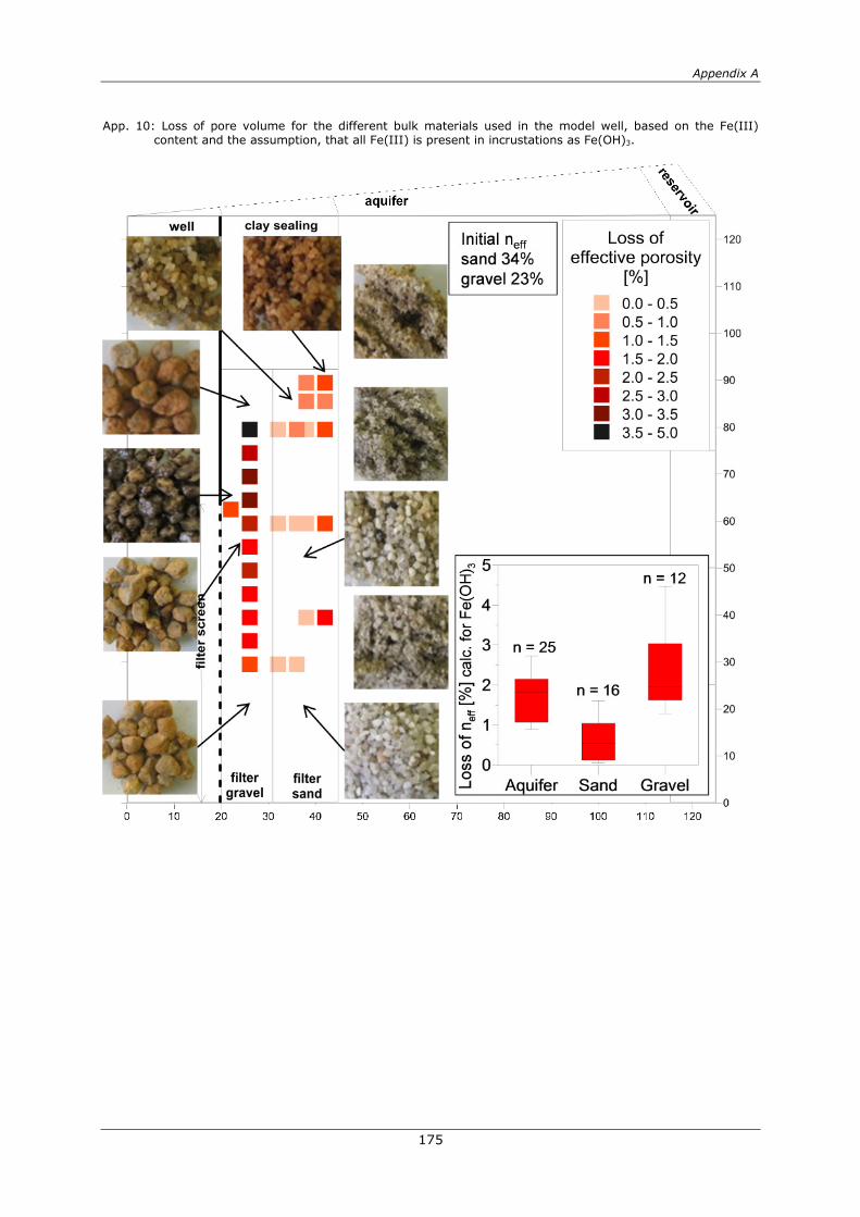
Appendix A
175
App. 10: Loss of pore volume for the different bulk materials used in the model well, based on the Fe(III) content and the assumption, that all Fe(III) is present in incrustations as Fe(OH)3.

Appendix A
176
Chapter 7
App. 11: Analysis of batch test deposits for different hydrogen peroxide concentrations and different treatment
intervals
0
4
8
12
16
20
ign
itio
n lo
ss
[%
]
1 bar
2 bar
0
0.1
0.2
0.3
0.4
flu
sh
ed
mate
rial
[g]
0.1 bar
1 bar
2 bar
no tre
atm
ent
0.0
3%
(2x)
0.3
0%
(2x)
3.0
0%
(2x)
no tre
atm
ent
0.0
3%
(2x)
0.3
0%
(2x)
3.0
0%
(2x)
no tre
atm
ent
0.0
3%
(2x)
0.3
0%
(2x)
3.0
0%
(2x)
H2O2 treatment
0
100
200
300
400
500
iro
n [
mg
]
1 bar
2 bar
column
no t
reatm
en
t
0.0
3%
(2
x)
0.3
0%
(2
x)
3.0
0%
(2x)
no t
reatm
en
t
0.0
3%
(2
x)
0.3
0%
(2
x)
3.0
0%
(2x)
no t
reatm
en
t
0.0
3%
(2
x)
0.3
0%
(2
x)
3.0
0%
(2x)
H2O2 treatment
0
4
8
12
ma
ng
an
es
e [
mg
]
1 bar
2 bar
column
0
0.01
0.02
0.03
0.04
0.05
ign
itio
n l
os
s [
g]
0.1 bar
1 bar
2 bar
t ) )t ) )t ) )t ) )t ) )
0
4
8
12
16
20
ign
itio
n lo
ss
[%
flu
sh
ed
ma
teri
al]
0.1 bar
1 bar
2 bar
no t
rea
tmen
t
0.3
0%
(1x)
0.3
0%
(2
x)
no t
rea
tmen
t
0.3
0%
(1x)
0.3
0%
(2
x)
no t
rea
tmen
t
0.3
0%
(1x)
0.3
0%
(2
x)
H2O2 treatment
0
100
200
300
400
500
iro
n [
mg
]
1 bar
2 bar
column
no
tre
atm
en
t
0.3
0%
(1
x)
0.3
0%
(2
x)
no
tre
atm
en
t
0.3
0%
(1
x)
0.3
0%
(2
x)
no
tre
atm
en
t
0.3
0%
(1
x)
0.3
0%
(2
x)
no
tre
atm
en
t
0.3
0%
(1
x)
0.3
0%
(2
x)
no
tre
atm
en
t
0.3
0%
(1
x)
0.3
0%
(2
x)
H2O2 treatment
0
20
40
60
80
100
iro
n [
%]
1 bar
2 bar
column

Appendix A
177
App. 12: Comparison of hydraulic conductivities from permeameter (batch columns) and associated material removal dependent on hydrogen peroxide concentration and treatment interval.
0 20 40 60 80 100
Σ flushed material [%]
0x100
10-3
2x10⁻³
3x10⁻³
4x10⁻³
kf [
m/s
]
H2O2 treatmentno treatment
0.03% (2x)
0.3% (2x)
3% (2X)
reference column kf = 3.7 . 10-3 [m/s]
0 20 40 60 80 100
Σ flushed material [%]
0x100
10-3
2x10⁻³
3x10⁻³
4x10⁻³
kf [
m/s
]
H2O2 treatmentno treatment
0.3% (1x)
0.3% (2x)
reference column kf = 3.7 . 10-3 [m/s]

Appendix A
178
Chapter 8
App. 13: Hydrochemical thresholds for well classification
Approach Method Options FRIe---22 STOborg15 TEGhzk-18
Distance to next
surface water
Estimation of main recharge
sources based on the
distance to surface water
bodies (river, lake, pond)
BF-GW-AR
Threshold: 100m
BF
70
BF-GW
100
BF-AR
170
Redox state of
recharge
Analysis of oxygen, redox
potential and iron in
observation wells located in
recharge areas (bank
filtrate, groundwater)
O2 [mg/L]: >0.1 - <0.1
- <0.01
Eh [mV]: >50>
Fe2+ [mg/L]: >0.2
0.31
95
0.7
0.02
27
1.4
0.00
80
0.5
Mixing rates
Shares of different recharge
sources in the abstracted
well water by stable isotopes
(18O, 2H) and temperature
time series
Shares of BF/AR [%]:
>70> high ~75% high ~70% -
Minimum travel
time Temperature drifts in well
months - years
Threshold: 6 to 12
months
BF: 3-4
months BF: years
BF: years
AR: months
Filter depth
Distance between top of the
filter screen and dynamic
water level
Low (<10m)
Medium (10-30m)
Large (>30m)
~15
medium
~5
low
~15
medium
Type of
pressure heads
Pump tests, bore logs,
hydrogeological profiles to
indentify hydraulic
conditions
Unconfined –
semiconfined - confined unconfined
semiconfine
d unconfined
Well location
Distance to neighboring
wells, central/peripheral
position within the well field
to assess impacts of well
interferences
Ø-distance to NW [m]
Threshold: 100m
Location: central -
peripheral
50
central
50
central
60
central

Appendix A
179
App. 14: Chosen factors and combinations and well performance data for the resulting well classes
Well classification Wells
(n)
Median residual well capacity
before 1st rehabilitation (%)
Median years of operation
before 1st rehabilitation
Single factors
1a Confined aquifer 148 76.62 16.35
1b Unconfined aquifer 210 68.47 11.06
2a Distance to water surface body < 100m 161 71.14 10.85
2b Distance to water surface body > 100m 171 76.70 14.67
3a Redox potential < 104.98 mV 137 68.20 10.63
3b Redox potential > 120.5 mV 167 76.84 12.26
4a Water level above well screen < 10m 29 59.94 8.17
4b Water level above well screen > 10m 365 72.88 11.31
Combinations
1a + 2a 71 69.51 21.98
1a + 2b 77 81.07 14.71
1b + 2a 137 68.74 11.22
1b + 2b 64 66.92 10.70
1a + 3a 43 73.02 14.80
1a + 3b 68 78.25 16.90
1b + 3a 68 60.31 12.64
1b + 3b 99 76.70 11.07
1a + 2a + 3a 23 69.37 22.85
1a + 2a + 3b 38 70.37 23.22
1a + 2b + 3a 20 80.40 14.54
1a + 2b + 3b 30 86.72 16.37
1b + 2a + 3a 24 61.80 8.09
1b + 2a + 3b 26 81.59 10.84
1b + 2b + 3a 40 59.10 14.88
1b + 2b + 3b 68 72.91 11.16
1a + 3a + 4a 3 96.37 26.94
1a + 3a + 4b 40 72.81 14.79
1a + 3b + 4a 1 72.00 20.53
1a + 3b + 4b 67 79.57 16.90
1b + 3a + 4a 15 58.10 8.14
1b + 3a + 4b 53 64.34 14.69
1b + 3b + 4a 4 76.10 8.27
1b + 3b + 4b 95 76.70 11.11


181


Publications
183
Publications
Technical papers
SCHWARZMÜLLER, H.; THRONICKER, O.; SZEWZYK, U.; MAIWALD, U.; MENZ, C.; TAUTE, T.; PEKDEGER, A.;
DLUBEK, H. (2009): Untersuchungen zur Reduzierung biochemischer Brunnenalterung. bbr Fachmagazin für Brunnen- und Leitungsbau 2009(12): 6
SCHWARZMÜLLER, H.; THRONICKER, O.; RAUCH, R.; SZEWZYK, U.; MAIWALD, U.; MENZ, C.; TAUTE, T.;
PEKDEGER, A.; DLUBEK, H. (2011): Eisenbakterien in Trinkwasserbrunnen. DVGW energie wasser-praxis(3): 16-19
MENZ, C.; SCHWARZMÜLLER, H.; TAUTE, T.; DLUBEK, H. (2013): Auswirkung unterschiedlicher
Schüttmaterialien auf die Verockerung und Regenerierbarkeit von Brunnen. bbr(4): 56-63
Conference contributions
SCHWARZMÜLLER, H.; TAUTE, T.; MENZ, C.; THRONICKER, O. (2010): Wie angewandte Forschung hilft, die Brunnenalterung zu verlangsamen (Ed.): Berliner Brunnentage, Pigadi GmbH, Potsdam, 31.05.-01.06.2010
MENZ, C.; TAUTE, T.; MAIWALD, U.; PEKDEGER, A. (2011): Impact of well operation on iron-related
clogging in quarternary aquifers in Berlin, Germany. IWA Specialist Groundwater Conference. Belgrade, 8-10 September 2011
SCHWARZMÜLLER, H.; THRONICKER, O.; MAIWALD, U.; MENZ, C.; TAUTE, T. (2012): Auslöser von
Alterungsprozessen in Brunnen und deren Verminderung im Betrieb (Ed.): 10. Berlin-Brandenburger Brunnentage Potsdam, pigadi
Reports
SCHWARZMÜLLER, H.; ORLIKOWSKI, D.; PEKDEGER, A.; TAUTE, T.; MAIWALD, U.; MENZ, C.; SZEWZYK, U.;
THRONICKER, O.; RAAT, K.; WICKLEIN, A.; BARTETZKO, A. (2011): Extended summary of the results and conclusions of the preparatory phase of the WellMa project. Kompetenzzentrum Wasser Berlin, 41 p. http://www.kompetenz-wasser.de/fileadmin/user_upload/pdf/forschung/WellMa/20111116_WELLMA1_Extended_summary_de.pdf
SCHWARZMÜLLER, H. & MENZ, C. (2013): WELLMA-2 Synthesis report. Kompetenzzentrum Wasser
Berlin, 37 p. http://www.kompetenz-wasser.de/fileadmin/user_upload/pdf/forschung/WellMa/D_6_WELLMA-2_Synthesis_report_v02.pdf


185
Acknowledgement
Since the start of this research, many people contributed to different phases of it. Firstly, I would like to thank Prof. Asaf Pekdeger and Dr. Thomas Taute for initiating this research and for giving me the possibility to contribute to this prolific study. I wished I had the chance to discuss my results with Prof. Pekdeger throughout the whole research phase, but I was pleased to do this with Tom instead. Especially, the study in France was a nice lesson to learn.
I would also like to thank my thesis referees Prof. Michael Schneider and Prof. Christoph Merz. Prof. Schneider never gived up hope and motivated me to finish my thesis.
Furthermore, I want to thank my colleagues at the FU Berlin for their support: Ulrike Maiwald for sharing office, work and thoughts, Fabian Hecht for his cross-disciplinary input, Andreas Winkler for his open door, Martin Recker for his active and patient technical support, Elke Heide for spending hours and days analysing samples, not forgetting all the students supporting the research studies. Thanks go to Almut Hilse, Julia Rücker, Sebastian Sklorz, Sascha Malarczuk, Fabius Markhoff, Ellen Schöne, Matthias Körting, David Muszynski, Alexander Könnecke, Alexander Meissner.
Next, I want to thank my colleagues at the KWB: Hella Schwarzmüller for taking the time to review my thesis and for her excellent quality management and Michael Rustler for his overwhelming useR-friendliness.
My thanks go also to the colleagues from BWB for cooperation and support, including Elke Wittstock, Gesche Grützmacher, Heidi Dlubek, Volker Jordan, Lutz Schmolke and Jan Loth.
I also thank BWB and Veolia for sponsoring this research.
Last but not least, I want to thank my family, who supported me throughout the last 8 years. From the beginning on, it was more than just a job and it had never come to an end, if you, Lisa, were not covering my back for so many times. Together with Jussi and Jonne it became a family project and I am very proud of what we had achieved.