Ownership characteristics and crop selection in California

Agriculture plays a major role in shaping California landscapes, and land ownership characteristics are an important predictor of

economic decision-making, conservation practices and recreational use (Ferranto et al. 2013; Macaulay 2016). As such, improved information on agricultural land ownership is necessary for continued improvements in agricultural efficiency and environmental protection. Although California has a robust history of collect-ing agricultural statistics at the county scale in county agricultural reports, these reports do not include information on the ownership characteristics of crop-land in their county, such as average property size, the distribution of ownership, and what kind of crops were planted together on individual properties.

Improvements in remote sensing technologies have allowed for increasingly accurate maps that specify where crops are planted, and advances in geographic information systems processing capacity is allowing for owner-level analysis of agricultural land use. This study presents a novel analysis that draws on publicly available satellite-based cropland data and a spatially explicit land ownership database that was developed by the authors.

The U.S. Department of Agriculture (USDA) Census of Agriculture surveys growers every 5 years and pro-vides substantial summary information on farms by acreage range and crop type. Our method supplements that data by providing information at the property

level, which we define as all parcels owned by a given landowner. This method allows the generation of own-ership summary statistics and measures of inequality by county and by crop. The method also provides new

RESEARCH ARTICLE

Ownership characteristics and crop selection in California croplandAnalyses of cropland ownership patterns can help researchers prioritize outreach efforts and tailor research to stakeholders’ needs.

by Luke Macaulay and Van Butsic

Online: https://doi.org/10.3733/ca.2017a0041

AbstractLand ownership is one of the primary determinants of how agricultural land is used, and property size has been shown to drive many land use decisions. Land ownership information is also key to understanding food production systems and land fragmentation, and in targeting outreach materials to improve agricultural production and conservation practices. Using a parcel dataset containing all 58 California counties, we describe the characteristics of cropland ownership across California. The largest 5% of properties — with “property” defined as all parcels owned by a given landowner — account for 50.6% of California cropland, while the smallest 84% of properties account for 25% of cropland. Cropland ownership inequality (few large properties, many small properties) was greatest in Kings, Kern and Contra Costa counties and lowest in Mendocino, Napa and Santa Clara counties. Of crop types, rice properties had the largest median size, while properties with orchard trees had the smallest median sizes. Cluster analysis of crop mixes revealed that properties with grapes, rice, almonds and alfalfa/hay tended to be planted to individual crops, while crops such as grains, tomatoes and vegetables were more likely to be mixed within a single property. Analyses of cropland ownership patterns can help researchers prioritize outreach efforts and tailor research to stakeholders’ needs.

Almond orchards in Stanislaus County. Analyzing land ownership distribution in California by crop type and property size can help scientists and extension professionals shape research programs according to the needs of local growers.

Luke

Mac

aula

y

http://calag.ucanr.edu • OCTOBER–DECEMBER 2017 221

https://doi.org/10.3733/ca.2017a0041

https://doi.org/10.3733/ca.2017a0041

http://calag.ucanr.edu

information on crop mixes by property, and presents the complex information in graphs and figures for ease of comprehension and further analysis.

Information about the property-size distribution and use of agricultural land at the property level is use-ful in assessing technology adoption, fragmentation of land, pesticide application, wildlife connectivity and many other issues (Brodt et al. 2006; Greiner and Gregg 2011; Sunding and Zilberman 2001). Data on agricul-tural landownership patterns can also help answer a host of important questions such as the characteristics of properties that are planted with a particular crop; variation in ownership patterns across counties; and

cropping combinations. Finally, ownership information also can be useful for organizations providing technical and conservation support on a landscape scale.

MethodsOwnership dataThe study describes California’s cropland. Private cropland includes land owned by private companies, individuals, nongovernmental organizations, and American Indian tribes (fig. 1A). Analyses were per-formed using two main datasets, a spatially explicit land ownership database and the USDA National

Private cropland Cropland acres0–5,0005,001–50,00050,001–200,000200,001–500,000500,001–1,062,000

Gini coefficient0.37–0.470.48–0.600.61–0.680.69–0.750.76–0.85

Acres of cropland by owner

5–150151–1,2751,276–125,000

Percent cropland0–0.50.6–1.71.8–6.36.4–3030.1–69.3

Mean cropland acres15–2627–5354–9697–153154–232

% Cropland largest owner controls

0.9–2.52.6–55.1–1010.1–3030.1–56.8

Number of owners0–150151–700701–1,8001,801–3,5003,501–8,462

Fig. 1. Descriptive measures of California cropland by count. Counties with gray shading have one or fewer cropland owners.

222 CALIFORNIA AGRICULTURE • VOLUME 71, NUMBER 4

Agricultural Statistics Service (NASS) Cropland Data Layer (CDL).

Parcel data was assembled for all 58 California counties. Parcel data with ownership information for 49 counties was derived from Boundary Solutions Inc., with the remaining nine counties assembled by con-tacting individual county governments. These county parcel data sets came from varying years, with 49 coun-ties from 2011 to 2015 and nine counties from 2005 to 2010. Although this does not provide a completely current ownership map at a single point in time, most counties have recent data. Additionally, studies indicate that only 0.5% of U.S. farmland is sold annually, sug-gesting that the impact of land sales on the results pre-sented here should be small (Sherrick and Barry 2003). In considering the ownership data presented here, it is also important to note that a sizeable percentage of landowners of California agricultural land (37%) are non-farming owners and rent or lease out their land to others (Bigelow et al. 2016).

To develop an ownership map for some counties, we merged data from separate files (nonspatial ownership information and spatial polygons) using a common field of assessor parcel numbers (APNs). After assem-bling county parcel maps for the entire state, we then dissolved parcels by owner name to remove interior borders of parcels owned by the same entity and to calculate total area under each ownership, which we refer to as a property. For analyses that used the county as the unit of analysis (section titled “County cropland ownership,” table 1 and fig. 1), the analysis only consid-ered ownership within that county. For all other analy-ses, ownerships were combined across all counties, so that land in multiple counties with a single owner was considered to be a single property.

Several counties had incomplete ownership data, and this initial mapping resulted in approximately 8% of the state’s area with unknown ownership in-formation (~8.25 million acres). To reduce the area of unknown ownership, we overlaid three separate own-ership maps that cover public land and conservation easements and used these maps to assign ownership to parcels that did not have ownership information from original parcel data (CCED 2015; CDFFP 2014; CPAD 2015). This process reduced unknown ownership to ap-proximately 2.7% of California’s total land area (~2.85 million acres) and 4.4% (~385,000 acres) of California’s cropland. Although unknown ownership is likely to be private, it was omitted from calculations. Ownerships were further categorized as public or private using 80 search terms in the ownership name field. The fi-nal ownership map was composed of approximately 543,495 properties greater than 5 acres across the state of California.

Cropland dataThe USDA CDL was used to assess crops grown in California. The CDL is a raster, geo-referenced, crop-specific land cover data layer with a ground resolution

of 30 meters. It is produced using satellite imagery from the Landsat 8 OLI/TIRS sensor and the Disaster Monitoring Constellation DEIMOS-1 and UK2 sen-sors collected during the 2013 growing season. The CDL methodology accommodates single and double crop plantings by using Farm Service Agency Common Land Unit data as training data. The CDL estimates occurrence of 99 different crops, which were con-densed by the authors to 14 broad crop categories. In making this classification, any single crop with more than 250,000 acres statewide was left as an individual crop type (see supplemental table 1 at ucanr.edu/u.cfm?id=182). The crop type grown on individual prop-erties was determined by overlaying the CDL with the spatial ownership database. The number of pixels of each particular crop type occurring within each own-ership boundary was calculated and converted to acres. The results provided in this analysis pertaining to crop category (tables 2 and 3) indicate the acres of crops grown within a property (rather than the total prop-erty size). Discussion of county-level results focuses on counties with more than 5,000 acres of cropland and more than 250 owners.

The CDL includes an accuracy assessment that includes the user’s accuracy and producer’s accuracy (USDA-NASS 2014). The user’s accuracy indicates the probability that a pixel from the CDL classification matches the ground truth data, while the producer’s accuracy indicates the probability that a ground truth pixel will be correctly mapped. We weighted the ac-curacies for all crop types based on their percentage of total cropland, resulting in a weighted average accuracy of 82% for both user and producer accuracy.

To reduce the effect of this error in the CDL, this study excluded properties smaller than 5 acres and those composed of less than 5% cropland, under the assumption that production of less than 5 acres, while possible, was not oriented towards production agri-culture and had a higher likelihood of being a remote sensing error. This exclusion reduced the overall private cropland area by 491,522 acres or 5.9%, resulting in a total private cropland area in this study of 7,872,543 acres. The number of owners was reduced more drasti-cally, dropping from 112,419 to 68,699, a reduction of

California Land Use and Ownership Portal

The authors, in collaboration with UC Agriculture and Natural Resources’ IGIS program, have also developed the California Land Use and Ownership Por-

tal, which has an interactive map displaying the information contained in this article and much more. The portal allows users to view each county’s cropland ownership and planting statistics as well as information about the natural veg-etation found in the county. This tool is useful for gaining a broad understand-ing of land use and land ownership at the county level in California. The portal allows users to export images, figures and charts of land ownership, crop cover and natural vegetation. You can access it at http://callands.ucanr.edu.


38.9%. Due to these reductions, we believe the esti-mates in this study to be conservative, while minimiz-ing the effect of remote sensing errors.

While we believe that our method of combining ownership and crop data produces a very high-quality map, some characteristics of the data influence the results and some error likely remains. Acreage sta-tistics are greatly affected by the cutoff value of the minimum size of cropland ownership (in this case 5 acres). Raising or lowering the minimum size farm in the dataset increases or decreases the mean and median statistics correspondingly. After evaluating various cutoff values, we felt that 5 acres was an ap-propriate cutoff that would include many of the small farmers in California, but minimize impacts of remote sensing error.

Another trend occurring in some parts of California that could affect results is the separation of large farm-ing operations into multiple corporate entities to re-duce liability risks. Although this practice would lead to a reduction in the mean acreage values, we don’t expect this practice to be widespread enough to sig-nificantly alter the results presented here. Additional sources of error include those arising from county level parcel data, from combining properties with very simi-lar names (as noted in the methods section below) and the aggregation of ownership maps over multiple years.

Additionally, the crop data is a snapshot in time. 2013 was a drought year, with likely many more acres left fallow than in a wetter year. Our analysis estimates fallow land at a total of 1.14 million acres. By compari-son, a previous analysis (NASA 2015) of 2011, a wetter year, estimated 500,000 acres of fallowed land. As such, our results should be viewed as reflecting dry year conditions, with reduced acreage planted to crops com-pared with an average or wetter year.

Analytical methodsSeveral analytical techniques are described that were used to prepare this data for analysis, includ-ing matching similar owner names, calculating equality metrics, and clustering properties based on planted crops.

Matching similar ownership names. In some cases, there were minor variations in owner names arising from different data entry protocols by county, punctuation standards, abbreviations and typographi-cal errors (for example “California State University” and “California State Univ”). To correct for these inconsistencies, we used the Jaro-Winkler distance measure (using a weight of p = 0.08, and a cutoff dis-tance value of < 0.05 for statewide matching and < 0.06 for county-level matching) to link records that have slightly different ownership names (Jaro 1989; Winkler 1990). The algorithm linked 14,459 records from the original dataset of 119,226 private cropland owner-ships. These linked records were combined and aggre-gated into 7,665 records. The combined records were evaluated for accuracy and resulted in an estimated TA

BLE

1. D

escr

iptiv

e m

easu

res

of C

alifo

rnia

priv

ate

crop

land

by

coun

ty

Coun

ty

Tota

l cr

op

acre

s

Num

ber

of

owne

rs

Perc

ent

crop

land

in

cou

nty

25th

pe

rcen

tile

Med

ian

acre

s75

th

perc

entil

e95

th

perc

entil

e

Larg

est

crop

ow

ners

hip

Perc

ent o

f cr

opla

nd

in la

rges

t ow

ners

hip

Aver

age

acre

sG

ini

coeffi

cien

tG

over

nmen

t ac

res

Unk

now

n ac

res

Ala

med

a6,

912

156

1.3%

1015

3916

161

38.

9%44

0.64

435

228

Alp

ine

179

10.

0%17

917

917

917

917

910

0.0%

179

0.00

Am

ador

4,82

612

11.

2%9

1734

149

663

13.7

%40

0.61

815

0

Butt

e24

5,03

22,

082

22.8

%10

2597

441

11,7

234.

8%11

80.

7516

,816

1,40

0

Cala

vera

s82

932

0.1%

1018

3767

809.

7%26

0.43

65

Colu

sa30

7,13

81,

694

41.5

%15

6420

970

64,

933

1.6%

181

0.67

5,22

282

9

Cont

ra C

osta

32,2

6842

56.

3%8

1536

201

7,49

923

.2%

760.

8129

El D

orad

o73

849

0.1%

712

1638

8711

.8%

150.

39

Fres

no1,

061,

382

8,46

227

.6%

1531

8259

811

,920

1.1%

125

0.75

13,3

4691

,892

Gle

nn23

7,53

51,

753

28.0

%15

3814

555

55,

954

2.5%

136

0.69

10,3

1213

,432

Hum

bold

t1,

501

200.

1%27

6499

188

240

16.0

%75

0.42

342

13,2

11

Impe

rial

411,

466

2,16

614

.3%

3381

190

632

31,0

127.

5%19

00.

6416

,767

23,2

92

Inyo

549

90.

0%22

2811

316

519

635

.8%

610.

521,

567

Kern

787,

189

3,64

215

.1%

1437

141

728

70,3

558.

9%21

60.

8141

,868

100,

531

King

s57

1,14

32,

457

64.1

%12

3311

664

411

3,96

920

.0%

232

0.85

37,7

7417

Lake

9,89

127

31.

2%8

1431

139

798

8.1%

360.

6410

2

Lass

en52

,306

384

1.7%

1336

137

610

2,31

44.

4%13

60.

712,

562

720

Los

Ang

eles

7,16

211

40.

3%9

1326

133

3,41

447

.7%

630.

7818

277

6

Mad

era

322,

758

2,17

823

.4%

1740

116

612

5,42

51.

7%14

80.

732,

472

2,19

2

Mar

in2,

073

600.

5%8

1435

110

280

13.5

%35

0.60

1,26

2

Mar

ipos

a69

40.

0%7

1323

3639

56.8

%17

0.41

710

Men

doci

no20

,921

513

0.9%

919

4214

864

43.

1%41

0.59

255

Mer

ced

483,

024

5,04

438

.2%

1527

7437

84,

425

0.9%

960.

728,

102

2,55

5

Mod

oc11

4,63

766

04.

3%29

8719

966

13,

614

3.2%

174

0.61

7,91

031

5

Mon

o3,

919

260.

2%35

9019

547

287

922

.4%

151

0.58

132

Mon

tere

y12

4,73

31,

202

5.9%

1438

9642

62,

385

1.9%

104

0.68

1,17

62,

625

Nap

a29

,849

880

5.9%

915

3112

374

52.

5%34

0.60

317

3,36

8

Nev

ada

135

80.

0%8

1318

3944

32.9

%17

0.37

Plac

er41

,980

401

4.4%

1021

9546

02,

589

6.2%

105

0.72

2,62

01,

171

Plum

as8,

738

530.

5%10

2811

098

82,

049

23.5

%16

50.

7715

89

Rive

rsid

e17

2,71

61,

969

3.7%

818

5231

710

,485

6.1%

880.

789,

795

134

Sacr

amen

to12

2,73

61,

313

19.3

%11

2991

362

3,78

93.

1%93

0.69

19,7

6217

,735

San

Beni

to26

,480

433

3.0%

1123

5920

72,

327

8.8%

610.

6617

13,

014

San

Bern

ardi

no1,

874

320.

0%10

3579

179

290

15.5

%59

0.55

2,32

25

San

Die

go31

116

0.0%

79

2458

7824

.9%

190.

5028

7

San

Joaq

uin

419,

338

5,13

446

.0%

1127

6829

98,

520

2.0%

820.

705,

904

62,3

64

San

Luis

Obi

spo

94,7

981,

391

4.5%

918

5026

66,

704

7.1%

680.

732,

044

13,2

68

San

Mat

eo46

918

0.1%

913

2771

149

31.6

%26

0.51

5

Sant

a Ba

rbar

a61

,611

1,16

43.

5%8

1849

188

1,77

82.

9%53

0.67

5,39

818

6

Sant

a Cl

ara

12,2

0237

31.

5%8

1634

116

383

3.1%

330.

5723

451

Sant

a Cr

uz3,

093

145

1.1%

814

2468

153

5.0%

210.

4630

24

Shas

ta28

,271

306

1.1%

821

9734

23,

947

14.0

%92

0.74

680

387

Sier

ra2,

345

390.

4%8

2565

168

484

20.6

%60

0.66

106

243

Sisk

iyou

146,

547

1,02

93.

6%14

4213

857

35,

772

3.9%

142

0.70

29,9

231,

521

Sola

no14

4,00

91,

235

24.7

%13

3711

544

15,

311

3.7%

117

0.70

1,27

687

4

Sono

ma

58,3

191,

401

5.7%

814

3114

52,

119

3.6%

420.

671,

133

1,86

9

Stan

isla

us29

1,36

95,

550

30.0

%10

2049

203

2,53

80.

9%52

0.64

4,28

917

,889

Sutt

er26

9,93

32,

221

69.3

%15

3712

950

76,

060

2.2%

122

0.69

5,91

63,

580

Teha

ma

67,5

691,

123

3.6%

814

3921

62,

950

4.4%

600.

7412

749

3

Trin

ity8

10.

0%8

88

88

100.

0%8

0.00

50

Tula

re66

4,39

26,

519

21.4

%12

2981

432

7,38

71.

1%10

20.

7220

,134

275

Tuol

umne

113

70.

0%5

625

4242

37.5

%16

0.47

1711

Vent

ura

4,32

522

80.

4%8

1324

4910

32.

4%19

0.41

104

107

Yolo

301,

554

1,97

646

.1%

1753

144

518

14,4

854.

8%15

30.

7119

,619

13,8

43

Yuba

100,

145

851

24.3

%10

3010

253

62,

425

2.4%

118

0.73

2,99

896

4


TABL

E 1.

Des

crip

tive

mea

sure

s of

Cal

iforn

ia p

rivat

e cr

opla

nd b

y co

unty

Coun

ty

Tota

l cr

op

acre

s

Num

ber

of

owne

rs

Perc

ent

crop

land

in

cou

nty

25th

pe

rcen

tile

Med

ian

acre

s75

th

perc

entil

e95

th

perc

entil

e

Larg

est

crop

ow

ners

hip

Perc

ent o

f cr

opla

nd

in la

rges

t ow

ners

hip

Aver

age

acre

sG

ini

coeffi

cien

tG

over

nmen

t ac

res

Unk

now

n ac

res

Ala

med

a6,

912

156

1.3%

1015

3916

161

38.

9%44

0.64

435

228

Alp

ine

179

10.

0%17

917

917

917

917

910

0.0%

179

0.00

Am

ador

4,82

612

11.

2%9

1734

149

663

13.7

%40

0.61

815

0

Butt

e24

5,03

22,

082

22.8

%10

2597

441

11,7

234.

8%11

80.

7516

,816

1,40

0

Cala

vera

s82

932

0.1%

1018

3767

809.

7%26

0.43

65

Colu

sa30

7,13

81,

694

41.5

%15

6420

970

64,

933

1.6%

181

0.67

5,22

282

9

Cont

ra C

osta

32,2

6842

56.

3%8

1536

201

7,49

923

.2%

760.

8129

El D

orad

o73

849

0.1%

712

1638

8711

.8%

150.

39

Fres

no1,

061,

382

8,46

227

.6%

1531

8259

811

,920

1.1%

125

0.75

13,3

4691

,892

Gle

nn23

7,53

51,

753

28.0

%15

3814

555

55,

954

2.5%

136

0.69

10,3

1213

,432

Hum

bold

t1,

501

200.

1%27

6499

188

240

16.0

%75

0.42

342

13,2

11

Impe

rial

411,

466

2,16

614

.3%

3381

190

632

31,0

127.

5%19

00.

6416

,767

23,2

92

Inyo

549

90.

0%22

2811

316

519

635

.8%

610.

521,

567

Kern

787,

189

3,64

215

.1%

1437

141

728

70,3

558.

9%21

60.

8141

,868

100,

531

King

s57

1,14

32,

457

64.1

%12

3311

664

411

3,96

920

.0%

232

0.85

37,7

7417

Lake

9,89

127

31.

2%8

1431

139

798

8.1%

360.

6410

2

Lass

en52

,306

384

1.7%

1336

137

610

2,31

44.

4%13

60.

712,

562

720

Los

Ang

eles

7,16

211

40.

3%9

1326

133

3,41

447

.7%

630.

7818

277

6

Mad

era

322,

758

2,17

823

.4%

1740

116

612

5,42

51.

7%14

80.

732,

472

2,19

2

Mar

in2,

073

600.

5%8

1435

110

280

13.5

%35

0.60

1,26

2

Mar

ipos

a69

40.

0%7

1323

3639

56.8

%17

0.41

710

Men

doci

no20

,921

513

0.9%

919

4214

864

43.

1%41

0.59

255

Mer

ced

483,

024

5,04

438

.2%

1527

7437

84,

425

0.9%

960.

728,

102

2,55

5

Mod

oc11

4,63

766

04.

3%29

8719

966

13,

614

3.2%

174

0.61

7,91

031

5

Mon

o3,

919

260.

2%35

9019

547

287

922

.4%

151

0.58

132

Mon

tere

y12

4,73

31,

202

5.9%

1438

9642

62,

385

1.9%

104

0.68

1,17

62,

625

Nap

a29

,849

880

5.9%

915

3112

374

52.

5%34

0.60

317

3,36

8

Nev

ada

135

80.

0%8

1318

3944

32.9

%17

0.37

Plac

er41

,980

401

4.4%

1021

9546

02,

589

6.2%

105

0.72

2,62

01,

171

Plum

as8,

738

530.

5%10

2811

098

82,

049

23.5

%16

50.

7715

89

Rive

rsid

e17

2,71

61,

969

3.7%

818

5231

710

,485

6.1%

880.

789,

795

134

Sacr

amen

to12

2,73

61,

313

19.3

%11

2991

362

3,78

93.

1%93

0.69

19,7

6217

,735

San

Beni

to26

,480

433

3.0%

1123

5920

72,

327

8.8%

610.

6617

13,

014

San

Bern

ardi

no1,

874

320.

0%10

3579

179

290

15.5

%59

0.55

2,32

25

San

Die

go31

116

0.0%

79

2458

7824

.9%

190.

5028

7

San

Joaq

uin

419,

338

5,13

446

.0%

1127

6829

98,

520

2.0%

820.

705,

904

62,3

64

San

Luis

Obi

spo

94,7

981,

391

4.5%

918

5026

66,

704

7.1%

680.

732,

044

13,2

68

San

Mat

eo46

918

0.1%

913

2771

149

31.6

%26

0.51

5

Sant

a Ba

rbar

a61

,611

1,16

43.

5%8

1849

188

1,77

82.

9%53

0.67

5,39

818

6

Sant

a Cl

ara

12,2

0237

31.

5%8

1634

116

383

3.1%

330.

5723

451

Sant

a Cr

uz3,

093

145

1.1%

814

2468

153

5.0%

210.

4630

24

Shas

ta28

,271

306

1.1%

821

9734

23,

947

14.0

%92

0.74

680

387

Sier

ra2,

345

390.

4%8

2565

168

484

20.6

%60

0.66

106

243

Sisk

iyou

146,

547

1,02

93.

6%14

4213

857

35,

772

3.9%

142

0.70

29,9

231,

521

Sola

no14

4,00

91,

235

24.7

%13

3711

544

15,

311

3.7%

117

0.70

1,27

687

4

Sono

ma

58,3

191,

401

5.7%

814

3114

52,

119

3.6%

420.

671,

133

1,86

9

Stan

isla

us29

1,36

95,

550

30.0

%10

2049

203

2,53

80.

9%52

0.64

4,28

917

,889

Sutt

er26

9,93

32,

221

69.3

%15

3712

950

76,

060

2.2%

122

0.69

5,91

63,

580

Teha

ma

67,5

691,

123

3.6%

814

3921

62,

950

4.4%

600.

7412

749

3

Trin

ity8

10.

0%8

88

88

100.

0%8

0.00

50

Tula

re66

4,39

26,

519

21.4

%12

2981

432

7,38

71.

1%10

20.

7220

,134

275

Tuol

umne

113

70.

0%5

625

4242

37.5

%16

0.47

1711

Vent

ura

4,32

522

80.

4%8

1324

4910

32.

4%19

0.41

104

107

Yolo

301,

554

1,97

646

.1%

1753

144

518

14,4

854.

8%15

30.

7119

,619

13,8

43

Yuba

100,

145

851

24.3

%10

3010

253

62,

425

2.4%

118

0.73

2,99

896

4


error rate of 4% based on a random sample of 100 linked names. Because only 12% of records were identi-fied for combining, in the context of the entire dataset the error rate of mistakenly combined records is 0.23% of all records. After this processing, the total number of owners with any cropland was 112,419.

Evaluating land concentration. For each county, we used the assembled ownership data to calculate the Gini coefficient of land ownership. The Gini coefficient

is a measure of statistical dispersion that is com-monly used as a measure of inequality. The coefficient values range from 0 to 1, where a value of 0 signifies perfect equality (every person owns the same amount of land) and a value near 1 equals perfect inequality (one individual owns all the land). The R package ineq (Zeileis 2014) was used to calculate Gini coefficients for each county.

Clustering of crop types. We used hierarchical clustering to evaluate combinations of crops planted together on a single property. Fourteen variables (representing 14 crop categories) were created cor-responding to the fraction of a property planted to a given crop category. We then standardized the values of these variables by subtracting the mean and divid-ing by the standard deviation. We ran a hierarchical cluster analysis that compares the dissimilarity of the 68,699 ownerships being clustered. In this method, each object is initially assigned to its own cluster and then the algorithm proceeds by joining the two most similar objects, continuing iteratively through the dataset until there is just a single cluster. We selected the Ward’s minimum variance method, which seeks to find compact spherical clusters using Euclidean distance, to cluster the ownerships based on mixes of crops present. We used the fastcluster package to im-plement the clustering algorithm, which has memory-saving routines and allowed for this analysis without creating a distance matrix (Müllner 2013). Caution should be taken in extrapolating 2013 crop mixes to other years, given that the analysis was performed during a drought year and farmers may have been making crop adjustments.

TABLE 2. Acres of government-owned cropland by crop type

Federal State LocalSpecial district

Miscellaneous government

Total acres

Alfalfa/hay 15,252 12,853 16,538 2,326 3,474 50,444

Almonds 2,358 1,169 3,363 1,363 139 8,393

Corn 408 3,429 1,597 600 10 6,044

Cotton 1,287 139 1,116 1,594 1,856 5,992

Fallow 48,222 46,704 25,325 34,121 6,303 160,675

Fruit trees 1,593 416 1,228 268 73 3,579

Grain crops 33,413 1,868 7,674 1,491 1,329 45,775

Grapes 312 1,024 2,347 709 19 4,410

Other tree crops

1,344 1,194 1,094 619 1 4,252

Rice 520 1,469 667 854 7 3,517

Tomatoes 916 162 538 699 1,170 3,484

Vegetables/fruit

4,810 1,435 1,240 771 634 8,891

Walnuts 1,016 375 1,214 1,011 264 3,881

Winter wheat 1,849 2,478 5,500 3,422 1,382 14,631

Total acres 113,302 74,715 69,440 49,846 16,663 323,967

TABLE 3. Descriptive statistics of crop types

Crop category

Total acres

Number of

owners25th

percentileMedian

acres75th

percentile95th

percentile

Largest crop

ownership

Percent of crop

in largest ownership

Average acres

Coefficient of variation

Gini coefficient

Alfalfa/hay 1,305,745 21,086 4.0 12.7 52.9 254.8 16,399 1.3% 61.9 3.7 0.76

Fallow 1,141,035 25,265 3.6 8.9 25.4 151.2 60,683 5.3% 45.2 10.3 0.80

Almonds 1,066,419 24,120 2.7 8.2 28.7 172.6 39,193 3.7% 44.2 7.4 0.80

Grapes 761,517 18,015 4.0 10.7 31.8 158.0 6,794 0.9% 42.3 3.5 0.76

Grain crops 674,197 13,214 3.3 12.0 46.9 205.1 12,153 1.8% 51.0 3.4 0.75

Rice 557,149 2,599 39.6 118.8 258.3 696.1 10,543 1.9% 214.4 1.9 0.61

Winter wheat

410,790 8,994 2.9 10.2 39.1 183.9 8,866 2.2% 45.7 3.3 0.76

Fruit trees 391,900 14,168 3.1 8.5 23.1 103.0 5,283 1.3% 27.7 3.5 0.73

Walnuts 313,258 11,284 2.2 6.7 22.7 115.2 8,225 2.6% 27.8 3.9 0.75

Cotton 277,694 2,374 5.8 30.5 98.3 340.4 56,602 20.4% 117.0 10.3 0.78

Tomatoes 272,021 4,051 3.3 14.7 69.8 299.7 3,179 1.2% 67.1 2.3 0.74

Corn 248,064 3,556 4.7 20.9 67.2 249.4 11,164 4.5% 69.8 3.8 0.73

Vegetables/fruit

247,844 4,891 4.7 15.8 55.3 203.3 3,655 1.5% 50.7 2.2 0.70

Other tree crops

203,908 5,779 1.6 5.3 16.9 134.8 14,275 7.0% 35.3 6.8 0.84


California crop-land ownership characteristicsApproximately 96% of California cropland is privately owned, followed by 1.4% federal, 0.9% state, 0.8% local and 0.6% special districts (e.g., ir-rigation districts). Of the government-owned land, 50% is fallow, 16% is alfalfa or hay and 14% is grain crops, with all other crops making up less than 5% of the total (table 2).

In 2013, there were ap-proximately 7.87 million acres of private cropland in California greater than 5 acres or 5% of an owner’s property, made up by approximately 68,699 owners. The largest 1% of cropland properties (the 687 properties larger than 1,277 acres) accounted for 26.5% of California’s cropland. The largest 5% of properties (3,435 proper-ties that are larger than 477 acres) account for just over half (50.6%) of California’s cropland. The remaining 95% of properties (65,370 properties) compose the remainder (49.4%) of the state’s cropland. The 25% of California cropland composed of the smallest properties is made up of 57,490 properties, 84% of all owners, and these prop-erties are less than 152 acres (table 4 and fig. 2). The median acreage of properties was 29.8 acres and mean acreage was 120.7 acres.

County cropland ownership We calculated metrics of cropland ownership on a county basis, including an analysis of equality of own-ership, represented by the Gini coefficient. Fresno, Kern and Tulare counties were the three counties with the largest overall area of cropland. Of the three, Kern County has the fewest number of properties (3,642 versus > 6,500). Two other counties, Sutter and Kings counties, were notable for their land area being domi-nated by cropland, with over 64% of their land area composed of private cropland, with the next highest amount at 46% in Yolo and San Joaquin Counties. Median size of cropland property tended to be larg-est in the rural corners of California, with the highest values in Imperial and Modoc counties (> 80 acres).

More urban and tourism-focused counties (Los Ange-les, Lake and Sonoma counties) tended to have lower median property size. Equality of cropland ownership, however, was not well-predicted by whether a county is rural or developed; rather, it tended to be most as-sociated with the size and number of the largest land-owners in the county or regulations implementing a minimum parcel size. Kings County has the most un-equal cropland ownership, followed by Kern and Con-tra Costa counties. The most equal cropland ownership (of counties with > 5,000 acres of private cropland) was found in Santa Clara, Napa and Mendocino counties (table 1 and fig. 1).

Crop typesMany crops had similar ownership characteristics with a few exceptions. Rice and cotton had large average acreages planted, while fruit trees, walnut trees and other tree crops had small average size plantings (table 3 and fig. 3).

Among properties growing rice, the average acres planted to rice were far larger (214 acres) than the aver-age acreages grown in all other crop categories. There were also few properties that planted small areas of

TABLE 4. Frequency table of ownership of California cropland based on size class

Size category (acres) Total acres

Percent of total acres

Cumulative sum of acres

Number of owners

Percent of total owners

Cumulative sum of owners

5–10 97,056 1.2% 97,056 13,327 19.4% 13,327

10–25 301,931 3.6% 398,988 18,413 26.8% 31,740

25–50 423,983 5.1% 822,970 11,853 17.3% 43,593

50–75 347,432 4.2% 1,170,402 5,573 8.1% 49,166

75–100 305,583 3.7% 1,475,985 3,572 5.2% 52,738

100–250 1,391,963 16.8% 2,867,948 8,875 12.9% 61,613

250–500 1,367,857 16.5% 4,235,805 3,934 5.7% 65,547

1,000 1,459,906 17.6% 5,695,711 2,106 3.1% 67,653

5,000 1,695,154 20.4% 7,390,865 975 1.4% 68,628

10,000 348,303 4.2% 7,739,168 51 0.1% 68,679

> 10,000 558,856 6.7% 8,298,024 20 0.03% 68,699

0%

10%

20%

30%

5−10 10−25 25−50 50−75 75−100 100−250 250−500 500−1,000 1,000−5,000

5,000−10,000

> 10,000

Size class (acres)

Perc

ent

% Owners in size class

% Cropland area in size class

19.4%

1.2%

26.8%

3.6%

17.3%

5.1%

8.1%

4.2%5.2%

3.7%

12.9%

16.8%

5.7%

16.5%

3.1%

17.6%

1.4%

20.4%

0.1%

4.2%

0.03%

6.7%

Fig. 2. Distribution of number of owners and percent of private cropland ownership greater than 5 acres in particular size classes of ownership.


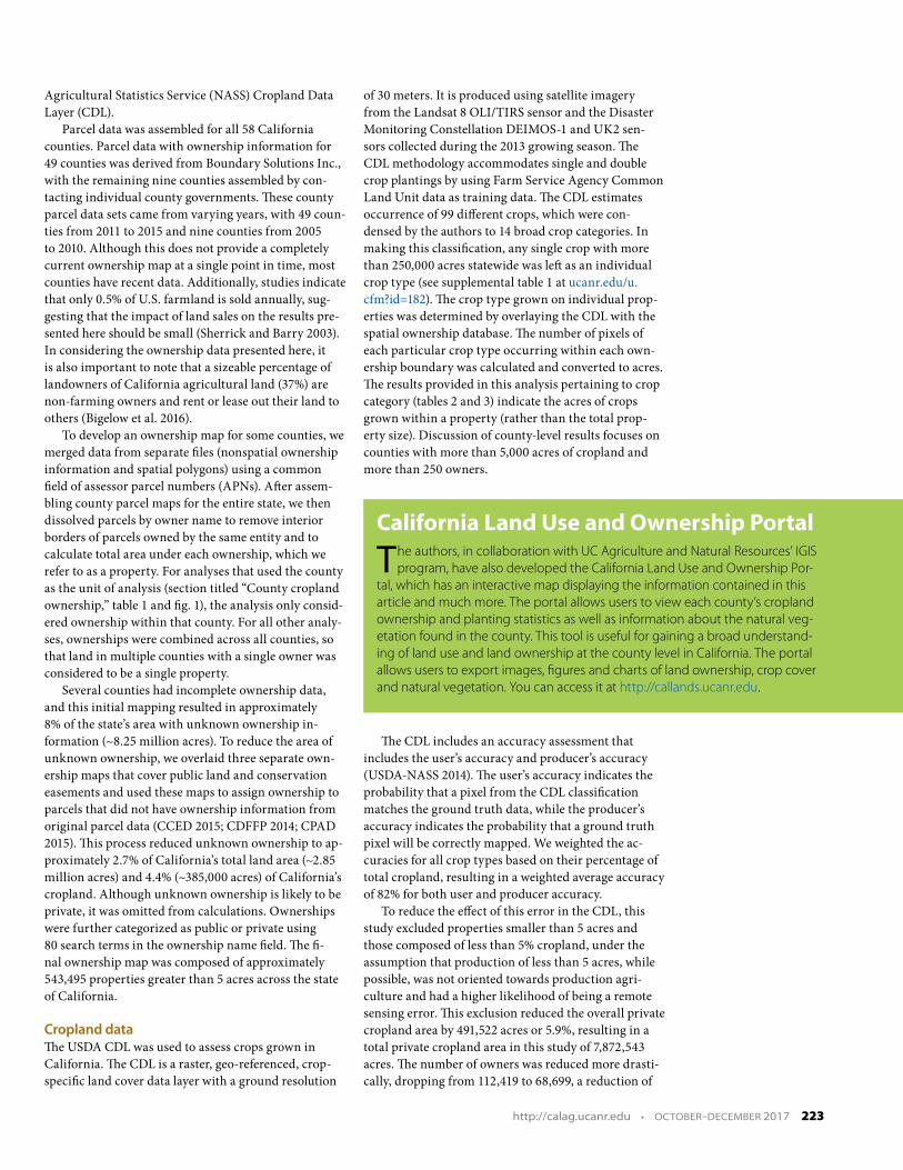
rice; the 25th percentile of rice acres planted was 40 acres, more than six times larger than the equivalent measure for any other crop type. Properties planted with cotton in 2013 had the second highest average (117 acres), but the median acreage of cotton properties was similar to other crops. The metric that tends to set cotton apart from rice is its much higher maximum acres grown on a single property (~56,600 acres). Rice and cotton had comparatively few properties planted, ranking 13th and 14th in number of owners across 14 crop categories, yet they ranked 6th and 10th in acres planted out of the crop categories.

The crop categories of fruit trees, walnuts and other tree crops were notable for their comparatively small ownerships. Mean ownership was between 27 and 35 acres, and median values were below 8.45 acres. While two other crop types, almonds and fallow land, had median values around 8 acres, their average values were comparatively larger.

The year 2013 was the second year of the recent and ongoing drought in California, and approxi-mately 25,265 owners had over a million acres left fallow, with 45 acres being the average area left fallow. Nearly 60,000 of those acres were left fallow by a sin-gle property owner in Kings, Kern and Tulare coun-ties, an area where crops grown are highly dependent on irrigation.

Land planted with rice, which had the highest average acreage planted, also had the most equal dis-tribution of land, in part because there were relatively few small properties. The most unequal ownership came in the other tree crops category, which is com-posed of 82% pistachios, 1% pecans and 17% all other tree crops. In that crop category, a single ownership that was planted with pistachios accounted for 7% of that crop category’s area. This, combined with an abundance of small owners (evidenced by the lowest median ownership size of all crop categories), led to a high inequality measure.

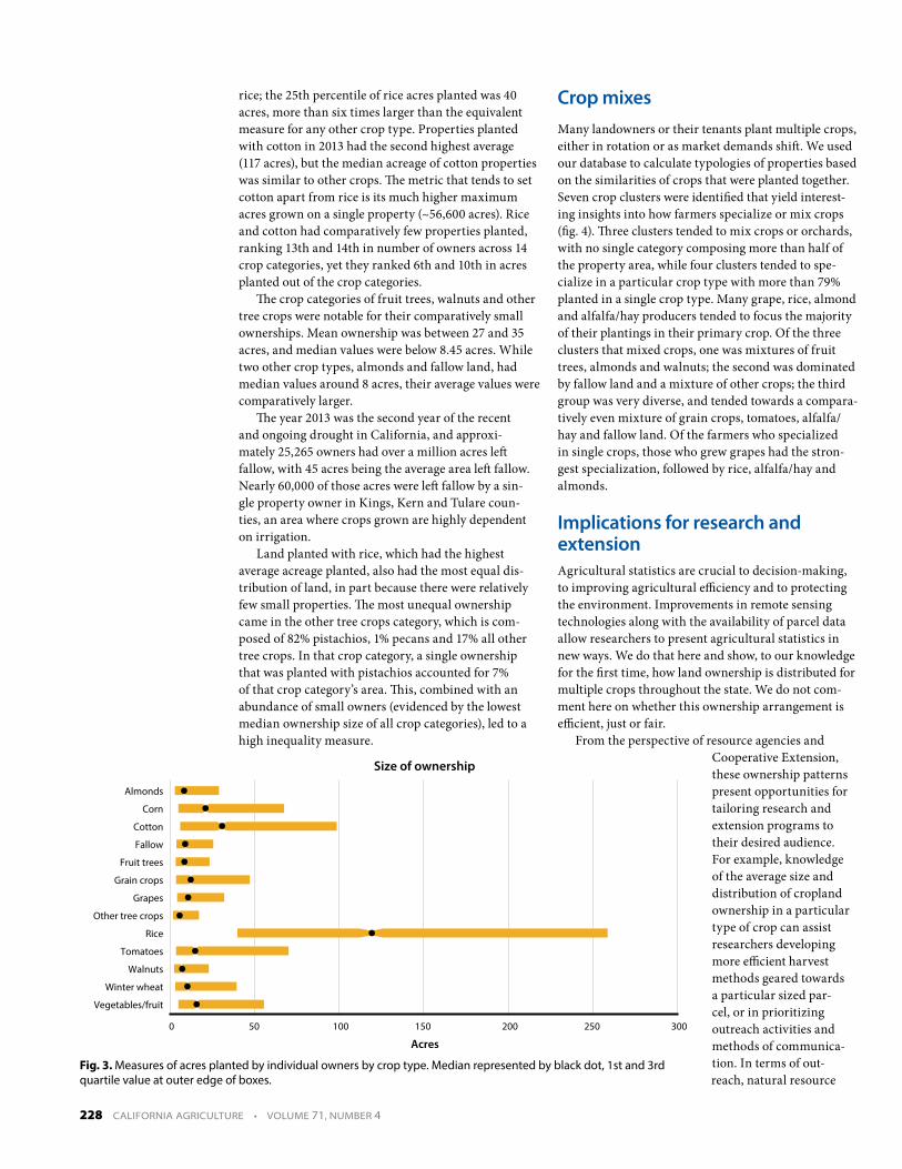
Crop mixesMany landowners or their tenants plant multiple crops, either in rotation or as market demands shift. We used our database to calculate typologies of properties based on the similarities of crops that were planted together. Seven crop clusters were identified that yield interest-ing insights into how farmers specialize or mix crops (fig. 4). Three clusters tended to mix crops or orchards, with no single category composing more than half of the property area, while four clusters tended to spe-cialize in a particular crop type with more than 79% planted in a single crop type. Many grape, rice, almond and alfalfa/hay producers tended to focus the majority of their plantings in their primary crop. Of the three clusters that mixed crops, one was mixtures of fruit trees, almonds and walnuts; the second was dominated by fallow land and a mixture of other crops; the third group was very diverse, and tended towards a compara-tively even mixture of grain crops, tomatoes, alfalfa/hay and fallow land. Of the farmers who specialized in single crops, those who grew grapes had the stron-gest specialization, followed by rice, alfalfa/hay and almonds.

Implications for research and extensionAgricultural statistics are crucial to decision-making, to improving agricultural efficiency and to protecting the environment. Improvements in remote sensing technologies along with the availability of parcel data allow researchers to present agricultural statistics in new ways. We do that here and show, to our knowledge for the first time, how land ownership is distributed for multiple crops throughout the state. We do not com-ment here on whether this ownership arrangement is efficient, just or fair.

From the perspective of resource agencies and Cooperative Extension, these ownership patterns present opportunities for tailoring research and extension programs to their desired audience. For example, knowledge of the average size and distribution of cropland ownership in a particular type of crop can assist researchers developing more efficient harvest methods geared towards a particular sized par-cel, or in prioritizing outreach activities and methods of communica-tion. In terms of out-reach, natural resource

Size of ownership

Acres

Vegetables/fruit

Winter wheat

Walnuts

Tomatoes

Rice

Other tree crops

Grapes

Grain crops

Fruit trees

Fallow

Cotton

Corn

Almonds

100500 200 300150 250

Fig. 3. Measures of acres planted by individual owners by crop type. Median represented by black dot, 1st and 3rd quartile value at outer edge of boxes.


professionals seeking to increase adoption of best practices in particular counties or for certain crop types can benefit from this knowledge. For example, in crop types dominated by a few large proper-ties, individual outreach may be an appropriate method of extension given the disproportion-ate area of cropland af-fected. Alternatively, crops dominated by many small properties like fruit trees or walnuts will likely require efforts utilizing mass communication tools that can reach thousands of owners. For crops with comparatively low varia-tion in ownership size (rice and tomatoes), outreach agencies may be able to reach a broad audience by focusing on challenges fac-ing an average sized farm. Crops with wide varia-tion in property size (e.g., almonds, other tree crops and properties with fallow land), may require an ap-proach that reaches own-ers of small, medium and large properties. While the vegetables/fruit category exhibits low variation in property size owned, it contains the widest varia-tion of crop types, requir-ing a large diversity of subject matter experts that can be devoted to relatively similar sized properties.

The analysis of crop mixes yields insights into guiding research and extension approaches, as well as information for equipment or seed sellers. Knowing that grapes, rice, alfalfa/hay and almonds all tended towards special-ization suggests that spe-cialized outreach may be most effective. Crop types that tend to be mixed may warrant the collaboration of researchers and advisors for synergies that can be gained in a mixed planting

system. The characteristics of the clusters can also help these collaborators know their audience; for example, properties with mixed crops from clusters 2 and 4 were

Fig. 4. Hierarchical clustering results based on the average percentages of crop category grown for each owner.

5.2% Almonds

85.2%Grapes

9.6% Other(12 types)

10.1% Alfalfa and hay

8.5% Corn

9.5% Fallow

30.0%Grain crops

8.6%Tomatoes

20.4% Winter wheat


11.2% Almonds

43.8%Fruit trees

27.2% Walnuts


6.5%Alfalfa and hay

6.4% Almonds

48.7%Fallow

8.3%Other tree crops

9.2% Vegs and fruits


87.5% Almonds


79.1% Alfalfa and hay

6.4% Almonds


6.8% Fallow83.0% Rice


#19,556 (13.9%) properties

786,053 acres (9.5%) of total cropland acres

#212,018 (17.5%) properties

2,031,278 acres (24.5%) of total cropland acres

#311,882 (17.3%) properties


#417,107 (24.9%) properties

2,430,631 acres (29.3%) of total cropland acres

#57,272 (10.6%) properties


#68,844 (12.9%) properties


#72,020 (2.9%) properties



larger than the average farm, while the tree crop mix (cluster 3) was composed of smaller properties than average.

The differences in distribution of ownership by different crop types or counties are likely influenced by the suitability of land for particular crops, histori-cal settlement patterns, whether economies of scale are present for growing the crop, and local land use ordinances. Walnuts had small median and mean area planted, which is likely driven by their requirements for high quality alluvial soils that occur along rivers flow-ing out of the Sierra Nevada. These lands have generally coincided with historic small towns that have been farmed for longer periods of time, leading to greater fragmentation as generations turn over and land hold-ings are split among family members (UC Agricultural Issues Center 1994a; Dr. Katherine Pope and Dr. David Ramos, UC Agriculture and Natural Resources, personal communication). Much of the state’s rice is grown on soils that have such a high clay content that no other crops can be productively grown on them, possibly reducing small-farm demand and subdivision for this type of land (UC Agricultural Issues Center 1994b; Dr. Jim Hill, UC Davis, personal communica-tion). The consolidation of cotton plantings occurred historically and likely is impacted by a variety of fac-tors, including the relative difficulty in growing cotton, its greater ability to grow in saline soils, and economies of scale in producing sufficient cotton to sustain a gin-ning operation (Dr. Robert Hutmacher, UC Agriculture and Natural Resources, personal communication).

The relative equality of ownership in counties like Santa Clara, Mendocino and Napa counties may be driven by earlier settlement and homesteading patterns where the size of farm was limited by the amount of

labor available (usually the immediate family), mak-ing large aggregations of acreage more difficult (Glenn McGourty, UC Agriculture and Natural Resources, personal communication). Additionally, Napa County enacted the Agricultural Preserve Act and Measure P, which implements minimum parcel size regulations and zones agricultural use as the best use in many areas of Napa County (Dr. Monica Cooper, UC Agriculture and Natural Resources, personal communication). These factors have led to comparatively few dominant landowners in these coastal agricultural areas, and in the case of Napa, fewer smallholders, which limits the measure of inequality.

These results provide useful information for Cooperative Extension efforts seeking to target growers by particular crop varieties or by various localities. This assessment can provide help in prioritizing outreach activities and methods of communication, as well as in tailoring research efforts to stakeholders’ needs. They may also prove useful in allocating resources regionally depending on the area of cropland, type of crop and number of people served. Continuing to track the rela-tionship between ownership patterns and crop patterns in the future will be a valuable way to analyze the ever-changing landscape of agriculture in California. c

L. Macaulay and V. Butsic are Assistant UC Cooperative Extension Specialists in the Department of Environmental Science, Policy and Management at UC Berkeley.

The authors thank the UC Berkeley Earth Sciences & Map Library and UC Agriculture and Natural Resources for funding to support this research.

ReferencesBigelow D, Borchers A, Hubbs T. 2016. US Farmland Ownership, Tenure, and Transfer. www.ers.usda.gov/publications/pub-details/?pubid=74675 (accessed Oct. 26, 2016).

Brodt S, Klonsky K, Tourte L. 2006. Farmer goals and man-agement styles: Implications for advancing biologically based agriculture. Agr Syst 89:90–105.

CCED [California Conservation Easement Database]. 2015. California Protected Areas Data Portal. www.calands.org/cced (accessed Apr. 28, 2016).

CDFFP [California Department of Forestry and Fire Protection]. 2014. FRAP - CAL FIRE Owner-ship Download. http://frap.fire.ca.gov/data/frapgisdata-sw-ownership13_2_download (ac-cessed Apr. 28, 2016).

CPAD [California Protected Ar-eas Database]. 2015. California Protected Areas Data Portal. www.calands.org/data (ac-cessed Apr. 28, 2016).

Ferranto S, Huntsinger L, Getz C, et al. 2013. Management without borders? A survey of landowner practices and at-titudes toward cross-boundary cooperation. Soc Natur Resour 26:1082–1100.

Greiner R, Gregg D. 2011. Farm-ers’ intrinsic motivations, barriers to the adoption of conservation practices and effectiveness of policy instruments: Empirical evidence from northern Austra-lia. Land Use Policy 28:257–65.

Jaro MA. 1989. Advances in record-linkage methodology as applied to matching the 1985 census of Tampa, Florida. J Am Stat Assoc 84:414–420.

Macaulay L. 2016. The role of wildlife-associated recreation in private land use and con-servation: Providing the miss-ing baseline. Land Use Policy 58:218–33.

Müllner D. 2013. fastcluster: Fast hierarchical, agglomerative clustering routines for R and Py-thon. J Stat Softw 53. www.jstat-soft.org/article/view/v053i09 (accessed Oct. 18, 2016).

NASA [National Aeronautics and Space Administration]. 2015. Federal agencies release data showing California Central Valley idle farmland doubling during drought. https://landsat.gsfc.nasa.gov/federal-agencies-release-data-showing-califor-nia-central-valley-idle-farmland-doubling-during-drought/ (accessed Mar. 11, 2017).

Sherrick BJ, Barry PJ. 2003. Farmland markets: Historical perspectives and contemporary issues. In: Moss CB, Schmitz A A(eds.). Government Policy and Farmland Markets. Ames, IA: Iowa State Press. p 27–49. http://onlinelibrary.wiley.com/doi/10.1002/9780470384992.ch3/summary (accessed Oct. 18, 2016).

Sunding D, Zilberman D. 2001. The agricultural innovation process: Research and technol-ogy adoption in a changing agricultural sector. Chapter 4. In: Handbook of Agricultural Eco-nomics. Vol. 1, part A. Gardner BL, Rausser GC (eds.). p 207–61.

UC Agricultural Issues Center. 1994a. The Walnut Industry in California: Trends, Issues and Challenges. University of Califor-nia, Agricultural Issues Center, Davis, Calif. http://aic.ucdavis.edu/publications/CAwalnuts.pdf (accessed Aug. 15, 2016).

UC Agricultural Issues Center. 1994b. Maintaining the com-petitive edge in California’s rice industry. University of California, Agricultural Issues Center, Davis, Calif. https://catalog.hathitrust.org/Record/100799847 (ac-cessed Aug. 15, 2016).

USDA-NASS [USDA National Agricultural Statistics Service]. 2014. 2013 California Cropland Data Layer. www.nass.usda.gov/Research_and_Science/Crop-land/metadata/metadata_ca13.htm (accessed Oct. 18, 2016).

Winkler WE. 1990. String comparator metrics and enhanced decision rules in the fellegi-sunter model of record linkage. http://eric.ed.gov/?id=ED325505 (ac-cessed Apr. 28, 2016).

Zeileis A. 2014. ineq: Measuring inequality, concentration, and poverty. https://CRAN.R-project.org/package=ineq.


http://www.ers.usda.gov/publications/pub-details/?pubid=74675



Documents

Ownership characteristics and crop selection in California