Overview of TM6: Simulation of Selenium Fate and

Transport in North San Francisco Bay

Limin Chen, Sujoy Roy, and Tom GriebTetra Tech, Inc., Lafayette, CA

Presentation to TMDL Advisory Committee

April 28, 2010

OverviewGoal: Develop tool to calculate selenium in water and biota in response to different loads of selenium entering North San Francisco Bay

Technical Review Process

Modeling Approach

Selenium Loads

Example Calibration Results

Predicted Loads and Concentrations

Role of Boundary Conditions

Model Scenarios

Technical Review Committee (2007-2010)

Dr. Nicholas S. Fisher, State University of New York, Stony BrookDr. Regina G. Linville, California State Office of Environmental Health Hazard AssessmentDr. Samuel N. Luoma, Emeritus, U.S. Geological SurveyDr. John J. Oram, San Francisco Estuary Institute

The role of the Technical Review Committee was to provide expert

reviews of the modeling process as well as credible technical advice on specific issues arising during the review.

Final TM-6 report includes their comments and our responses.

Model Structure

Total Particulate Selenium as a Mix of Organic and Inorganic Species (μg/g)

Uptake by bivalves

Uptake by predator species

ECoSModel

Results

DYMBAMModel

TTF

SelenateDSe(VI)

SeleniteDSe(IV)

Organic SelenideDSe(-II)

Selenate +Selenite

PSe(IV+VI)

Elemental SePSe(0)

Organic SelenidePSe(-II)

Bed Sediments

Dissolved species

Particulate species

Point Sources (Refineries, POTWs, Other Dischargers)

Contribute primarily to suspended particulates, and to dissolved phase in a limited way

Contribute to dissolved phase

Estuary Water Column

River and Tributary

Loads

SelenateDSe(VI)

SeleniteDSe(IV)

Organic SelenideDSe(-II)

Selenate +Selenite

PSe(IV+VI)

Elemental SePSe(0)

Organic SelenidePSe(-II)

Bed Sediments

Dissolved species

Particulate species

Point Sources (Refineries, POTWs, Other Dischargers)

Contribute primarily to suspended particulates, and to dissolved phase in a limited way

Contribute to dissolved phase

Estuary Water Column

River and Tributary

Loads

Total Particulate Selenium as a Mix of Organic and Inorganic Species (μg/g)

Uptake by bivalves

Uptake by predator species

ECoSModel

Results

DYMBAMModel

TTF

SelenateDSe(VI)

SeleniteDSe(IV)

Organic SelenideDSe(-II)

Selenate +Selenite

PSe(IV+VI)

Elemental SePSe(0)

Organic SelenidePSe(-II)

Bed Sediments

Dissolved species

Particulate species

Point Sources (Refineries, POTWs, Other Dischargers)

Contribute primarily to suspended particulates, and to dissolved phase in a limited way

Contribute to dissolved phase

Estuary Water Column

River and Tributary

Loads

SelenateDSe(VI)

SeleniteDSe(IV)

Organic SelenideDSe(-II)

Selenate +Selenite

PSe(IV+VI)

Elemental SePSe(0)

Organic SelenidePSe(-II)

Bed Sediments

Dissolved species

Particulate species

Point Sources (Refineries, POTWs, Other Dischargers)

Contribute primarily to suspended particulates, and to dissolved phase in a limited way

Contribute to dissolved phase

Estuary Water Column

River and Tributary

Loads

ECoS = Fate and transport modeling framework for selenium species

DYMBAM = Dynamic Bioaccumulation Model for estimating bivalve concentrations

TTF = Trophic Transfer Factor, ratio between food and predator tissue concentration

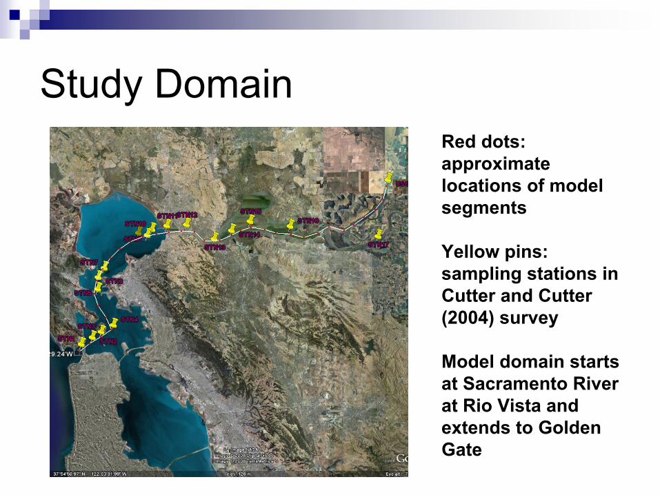
Red dots: approximate locations of model segments

Yellow pins: sampling stations in Cutter and Cutter (2004) survey

Model domain starts at Sacramento River at Rio Vista and extends to Golden Gate

Study Domain

Model Components and Steps in Calibration1.

Salinity: relatively conservative (advection and dispersion)2.

Total Suspended Material: three components of PSP, BEPS and phytoplankton, result of advection, dispersion

3.

Phytoplankton (Chl a): result of advection, dispersion, growth, respiration, and grazing

4.

Dissolved selenium: selenite (SeIV), organic selenide (SeII), selenate (SeVI)

5.

Particulate selenium: particulate elemental , particulate organic selenide , particulate adsorbed selenite + selenate

Transformation modeled as first order reactions; transformations

include: uptake by phytoplankton, adsorption/desorption, oxidation, mineralization

Modeling StepsDuring model calibration, adjustable parameters were varied to obtain a best fit to the data; for evaluation, the model was run with the fitted parameters and compared with new data setsModel calibrated to data from 1999, and tested against datasets from 2001, 2005, 1998 and 1986Model applied in a predictive mode using historical hydrology and different load scenariosTetra Tech worked with model developers (Shannon Meseck, John Harris) over the course of this work

Model Schematic

Point Sources, Tributaries, and South Bay Input

Sacramento River at Rio Vista

San Joaquin River near

Delta

Seawater Exchange

North San Francisco BayGolden Gate

1-D model with 33 well-mixed cells representing the bay.

Selenium Transformations

SelenateSe(VI)

Organic Selenide

Se(-II)

SeleniteSe(IV)

Dissolved SpeciesSelenate+ Selenite

Se(VI)+ Se(IV)

Organic Selenide

Se(-II)

Elemental SeSe(0)

Selenate+ SeleniteSe(VI)+ Se(IV)

Organic Selenide

Se(-II)

Elemental SeSe(0)

Organic SelenideSe(-II)

PSP

Phyto-plankton

BEPS

Mineralization, k1

Uptake, k6

Mineralization, k 1

Mineralization, k1Ads/Des, a’, b

Ads/Des, a

’, b

Uptake, k4

Uptake, k5

Oxidation, k2

Oxidation, k3

Advective/Dispersive Exchange with Upper

Cell

Advective/Dispersive Exchange with Lower

Cell

Bed Exchange

Represented by first-order rate constants.

Uptake by Bivalves

Time

Time

Time

Time

Se(0), particulate

Se(IV) + Se(VI),particulate

Se(-II),particulate

AE = 0.2AE = 0.45

AE = 0.54 to 0.8

C. amurensisconcentration

CmsskeCfIRAECwkudtdCmss ×−××+×=

Cmss

is selenium concentration in tissue (μg/g), ku

is the dissolved metal uptake rate constant (L/g/d), Cw

is the dissolved metal concentration (µg/L), AE is the assimilation efficiency (%), IR is the ingestion rate (g/g/d), Cf

is the metal concentration in food (e.g. phytoplankton, suspended particulate matter, sediment) (µg/g), and ke

is the efflux rate (d-1).

Boundary Conditions are Important

0 100Distance

C

Sources in the Bay

Seawater boundary

Riverine boundary

C, on the y-axis, represents a constituent being modeled. The model framework shown on the preceding slides involves the solution of a set of differential equations. These explain the shape of the curve. However, the boundary conditions also have an important effect on determining the actual magnitudes of C.

Year

1985 1990 1995 2000 2005

Sel

eniu

m lo

ads

(kg/

yr)

0

2000

4000

6000

8000

10000

Riverine (kg/yr) Refineries (kg/yr) Tributaries (kg/yr)

Annual Selenium Loads

Dissolved Loads for Water Year 1999

SJR @ Vernalis2666

7%Delta 365

South Bay1607 176

SJR @ confluence POTWs32% 3%

Sac. River @ Rio Vista Bay Exchange with Ocean Water1502 503430%

Tributaries Refineries820 55916% 11%

Particulate Loads for Water Year 1999

SJR @ Vernalis652

Delta

78 0SJR @ confluence POTWs

11%

Sac. River @ Rio Vista Bay Exchange with Ocean Water465 ~ 754 804 (32 BEPS)

89%Tributaries Refineries Bed Exchange

0 0 0.1

⎟⎟

⎠

⎞

⎜⎜

⎝

⎛−−=

∑∑

∑∑

XcalXobs

XobsXcal

GOF 1*100(%)

Example Calibration 1: Salinity (1999)

Salinity

Observed (psu)

0 5 10 15 20 25 30 35Pr

edic

ted

(psu

)0

5

10

15

20

25

30

35

y = 0.9272 x + 1.0404

Jan 21, 1999

Salin

ity (p

su)

0

5

10

15

20

25

30

35

April 14, 1999

Salin

ity (p

su)

0

5

10

15

20

25

30

35

May 7, 1999

Salin

ity (p

su)

0

5

10

15

20

25

30

35

June 7, 1999

Distance (km)

0 20 40 60 80 100

Salin

ity (p

su)

0

5

10

15

20

25

30

35

August 17, 1999

Sep 14, 1999

Oct 19, 1999

Nov 10, 1999

Distance (km)

0 20 40 60 80 100

r = 1.00GOF = 97.0%

r = 0.98GOF = 99.6%

r = 1.00GOF = 89.2%

r = 0.97GOF = 85.2%

r = 0.99GOF = 98.5%

r = 1.00GOF = 94.9%

r = 1.00GOF = 94.8%

r = 0.99GOF = 97.5%

Example Calibration 2: Chlorophyll a (1999)

Jan 21, 1999

Chl

a ( μ

g/L)

0

2

4

6

8

10

12

April 14, 1999

Chl

a ( μ

g/L)

0

2

4

6

8

10

12

May 7, 1999

Chl

a ( μ

g/L)

0

2

4

6

8

10

12

June 7, 1999

Salinity

0 5 10 15 20 25 30 35

Chl

a ( μ

g/L)

0

2

4

6

8

10

12

August 17, 1999

0

2

4

6

8

10

12

Sep 14, 1999

0

2

4

6

8

10

12

Oct 19, 1999

0

2

4

6

8

10

12

Nov 10, 1999

Salinity

0 5 10 15 20 25 30 350

2

4

6

8

10

12

r = 0.31GOF = 68.5%

r = 0.09GOF = 95.2%

r = 0.40GOF = 92.4%

r = 0.47GOF = 86.0%

r = 0.45GOF =66.8%

r = -0.04GOF = 48.2%

r = 0.07GOF = 31.8%

r = 0.83GOF = 82.2%

Chlorophyll a

Observed (μg/L)

0 2 4 6 8 10 12 14 16P

redi

cted

(μg/

L)

0

2

4

6

8

10

12

14

16

R2 = 0.358

Salinity

0 5 10 15 20 25 30 35

Sel

enite

(μg/

L)

0.00

0.02

0.04

0.06

0.08

0.10

Salinity

0 5 10 15 20 25 30 35

Sel

enat

e (μ

g/L)

0.00

0.02

0.04

0.06

0.08

0.10

Salinity

0 5 10 15 20 25 30 35

Org

. Sel

enid

e (μ

g/L)

0.00

0.02

0.04

0.06

0.08

0.10

r = 0.164GOF= 95.0%

r = 0.192GOF = 78.3%

r = 0.353GOF = 95.8%

Example Calibration 3: Dissolved Selenium (1999)

Salinity

0 5 10 15 20 25 30 35

Par

t. S

eIV

+SeV

I (μg

/L)

0.000

0.005

0.010

0.015

0.020

0.025

Salinity

0 5 10 15 20 25 30 35

Par

t. S

e0 (μ

g/L)

0.000

0.005

0.010

0.015

0.020

0.025

Salinity

0 5 10 15 20 25 30 35

Par

t. S

e-II

(μg/

L)

0.000

0.005

0.010

0.015

0.020

0.025

r = 0.801GOF = 92.1%

r = 0.676GOF = 83.5%

r = -0.021GOF = 73.5%

Example Calibration 4: Particulate Selenium (1999)

TSM Long-Term Evaluation at USGS Stations

STN 3

1998 2000 2002 2004 2006 2008 2010

TSM

(mg/

l)

0

50

100

150

200

250ObservedSimulated

STN 6

Year

1998 2000 2002 2004 2006 2008 2010

TSM

(mg/

l)

0

50

100

150

200

250

ObservedSimulated

STN 14

1998 2000 2002 2004 2006 2008 2010

TSM

(mg/

l)

0

50

100

150

200

250

ObservedSimulated

STN 18

Year

1998 2000 2002 2004 2006 2008 2010

TSM

(mg/

l)

0

50

100

150

200

250

ObservedSimulated

Evaluation of Chlorophyll a STN 3

1998 2000 2002 2004 2006 2008 2010

Chl

a ( μ

g/l)

0

2

4

6

8

10

12

14

16

18

20ObservedSimulated

STN 6

Year

1998 2000 2002 2004 2006 2008 2010

Chl

a ( μ

g/l)

0

2

4

6

8

10

12

14

16

18

20ObservedSimulated

STN 14

1998 2000 2002 2004 2006 2008 2010

Chl

a ( μ

g/l)

0

10

20

30

40

50

ObservedSimulated

STN 18

Year

1998 2000 2002 2004 2006 2008 2010

Chl

a ( μ

g/l)

0

2

4

6

8

10

12

14

16

18

20ObservedSimulated

Suisun Bay

Suisun Bay

San Pablo Bay

Central Bay

Predicted Particulate Selenium Concentrations (1999)

November 11, 1999

0 5 10 15 20 25 30 35

Par

t. Se

IV +

SeV

I (μg

/g)

0.0

0.1

0.2

0.3

0.4

0.5

0.6

0.7

0.8

ObservedPredicted

0 5 10 15 20 25 30 35

Part.

Se0

( μg/

g)

0.0

0.1

0.2

0.3

0.4

0.5

0.6

0.7

0.8

0 5 10 15 20 25 30 35

Par

t. Se

II ( μ

g/g)

0.0

0.1

0.2

0.3

0.4

0.5

0.6

0.7

0.8

Salinity

0 5 10 15 20 25 30 35

Tota

l Par

t. Se

( μg/

g)

0.2

0.4

0.6

0.8

1.0

1.2

1.4

1.6

1.8

Bivalve (C. amurensis) Concentrations

Year

1998 1999 2000 2001 2002 2003 2004 2005 2006

Cm

ss (μ

g/g)

0

5

10

15

20

25ObservedIR = 0.45, AE = 0.2,0.45, 0.8IR = 0.65, AE = 0.2, 0.45, 0.8IR = 0.65, AE = 0.2, 0.45, 0.54IR = 0.85, AE = 0.2, 0.45, 0.80

White Sturgeon Concentrations

Year

80 85 90 95 00 05 10

Mus

cle

sele

nium

con

cent

ratio

n (μ

g/g)

0

10

20

30

40

50

Suisun BaySan Pablo BayEstuary Mean

TTF = 1.7

Effect of Changing Boundary Conditions

Salinity

0 5 10 15 20 25 30 35

Part

icul

ate

Sele

nium

( μg/

g)

0.00.20.40.60.81.01.21.41.61.8

ObservedLower BoundaryHigher Boundary

Scenarios Examined

Scenario Description1 Base case

2 Removal of all point source loads (refineries, POTWs), and local tributary loads

3 30% reduction in refinery and San Joaquin River loads, dissolved only

4 50% reduction in all point sources (refineries, POTWs), local tributaries and San Joaquin River loads, dissolved only

5 Increase dissolved selenium loads from San Joaquin River by a factor of 3, particulate loads remain the same as the base case

6 Decrease dissolved selenium loads from San Joaquin River by a factor of 50%, particulate loads remain the same as the base case

7 Increase particulate selenium loads associated with PSP, BEPS, and phytoplankton from Sacramento River by a factor of 3, dissolved loads remain the same as the base case

8 Decrease particulate selenium loads associated with PSP, BEPS, and phytoplankton from Sacramento River by a factor of 50%, dissolved loads remain the same as the base case

9 Increase San Joaquin River particulate loads by 3x, other loads stay the same

10 A natural load scenario, where the point sources are zero, the local tributary loads and speciation are at Sacramento River values, and the San Joaquin River is at 0.2 µg/l, at current speciation

Impact on Dissolved Se

High Flow Month (April, 1999)

0 1 2 3 4 5 6 7 8 9 10

Dis

solv

ed S

e ( μ

g/l)

0.0

0.1

0.2

0.3

Low Flow Month (November, 1999)

0 1 2 3 4 5 6 7 8 9 10

Dis

solv

ed S

e (μ

g/l)

0.0

0.1

0.2

Dry Year Dry Month (July, 2001)

0 1 2 3 4 5 6 7 8 9 10

Dis

solv

ed.S

e (μ

g/l)

0.0

0.1

0.2

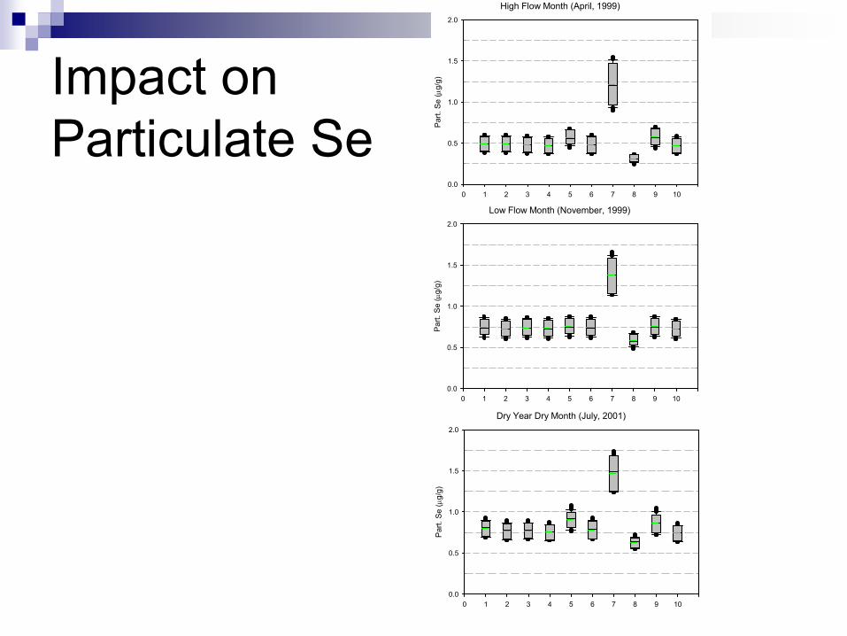
Impact on Particulate Se

High Flow Month (April, 1999)

0 1 2 3 4 5 6 7 8 9 10

Par

t. S

e (μ

g/g)

0.0

0.5

1.0

1.5

2.0

Low Flow Month (November, 1999)

0 1 2 3 4 5 6 7 8 9 10

Par

t. S

e (μ

g/g)

0.0

0.5

1.0

1.5

2.0

Dry Year Dry Month (July, 2001)

0 1 2 3 4 5 6 7 8 9 10

Par

t. S

e (μ

g/g)

0.0

0.5

1.0

1.5

2.0

Summary of Model ResultsThe model is able to simulate key aspects of physical and biological constituents that affect selenium concentrations.During calibration, the model was able to fit the patterns in concentrations of dissolved and particulate selenate and selenite well, although it performed less well for the organic fractions. The model was also able to represent the observed variation in biota concentrations.The model is a valuable tool to explore selenium transport, fate, and bioaccumulation in the bay, and can be applied in analyses in support of the TMDL, as demonstrated through a set of example scenarios.A modeling study provides an opportunity to synthesize information from the system, and in doing so, highlights unknowns that may have a bearing on model predictions. This report presents a set of data needs for further evaluation such as characterization of boundary conditions, selenium loads from major sources, recent water column concentrations and speciation, as well as biota concentrations.

Impact on Bivalve Se

High Flow Month (April, 1999)

0 1 2 3 4 5 6 7 8 9 10

Cm

ss S

e ( μ

g/g)

0

5

10

15

20

25

30

35

Low Flow Month (November, 1999)

0 1 2 3 4 5 6 7 8 9 10

Cm

ss S

e (μ

g/g)

0

5

10

15

20

25

30

35

Dry Year Dry Month (July, 2001)

0 1 2 3 4 5 6 7 8 9 10

Cm

ss S

e (μ

g/g)

0

5

10

15

20

25

30

35