Overview of Methods for Measurement of Track ... · PDF fileOverview of Methods for Measurement of Track Irregularities ... coach, matrix elements ... rail contact in the frequency

RIVAS

SCP0-GA-2010-265754

RIVAS_CHALMERS_ WP2_D2_5 Page 1 of 49 2/7/2013

RIVAS

Railway Induced Vibration Abatement Solutions

Collaborative project

Overview of Methods for Measurement of Track Irregu larities

Important for Ground-Borne Vibration

Deliverable D2.5

Submission date: 02/07/2013

Project Coordinator:

Bernd Asmussen

International Union of Railways (UIC)

[email protected]

RIVAS

SCP0-GA-2010-265754


Title Overview of Methods for Measure ment of Track Irregularities Important for Ground-Borne Vibration

Domain WP 2

Date 02/07/2013

Author/Authors Jens Nielsen, Eric Berggren, Thomas Lölgen, Roger Müller, Bert Stallaert, Lise Pesqueux

Partner Chalmers University of Technology, Trafikverket, DB, SBB, D2S International, Alstom

Document Code RIVAS_CHALMERS_ WP2_D2_5 Version 2 Status Final

Dissemination level:

Document history

Revision Date Description

1 17/4/2013 Draft Version

2 2/7/2013 Final Version Approved by Bernd Asmussen

Project co-funded by the European Commission within the Seventh Framework Programme

Dissemination Level PU Public X PP Restricted to other programme participants (including the Commission Services) RE Restricted to a group specified by the consortium (including the Commission) Services) CO Confidential, only for members of the consortium (including the Commission Services)

RIVAS

SCP0-GA-2010-265754


1. EXECUTIVE SUMMARY

The dynamic component of vertical wheel–rail contact forces, as induced by irregularities in track geometry (longitudinal level, isolated rail defects, welds, insulated joints, rail corrugation, switches & crossings, etc) and track stiffness (transition zones, hanging sleepers, culverts, etc), is an important source to ground-borne vibration and ground-borne noise.

Thus, one important aspect of controlling vibration levels is the availability of systems that accurately measure and monitor vertical track (and rail) irregularities to facilitate maintenance management. Such systems are surveyed in this report, covering methods measuring unloaded or loaded track irregularities in the wavelength interval relevant for the excitation of ground-borne vibration and noise. The main features of the different systems are listed and pros and cons are discussed.

Unfortunately, none of the available systems measures the complete wavelength interval relevant for ground-borne vibration and ground-borne noise. For example at a conventional freight train speed of 80 km/h, the relevant wavelengths are from around 0.1 m up to about 10 m. In common practice and according to existing standards, track recording coaches (TRC) are used to assess loaded track geometry (longitudinal level) with wavelengths down to 3 m (sometimes 1 m), whereas hand-held accelerometer-based trolleys and mechanical displacement probes measure unloaded rail irregularities up to about 0.5 m. To cover the complete wavelength interval, a combination of measurement methods is required.

To improve the monitoring of longitudinal level at wavelengths important for ground-borne vibration and noise, it is suggested to introduce a new wavelength band (here it is referred to as D0, c.f. the EN standard 13848) containing wavelengths in the interval 0.5 – 3 m. Together, the D0 and D1 bands correspond to excitation frequencies in the range 0.9 – 44 Hz at vehicle speed 80 km/h (2 – 110 Hz at 200 km/h). Many existing TRC already have the capability required to measure wavelengths down to 0.5 m but a filtering of data is generally applied to meet existing standards (wavelengths of interest are down to 3 m, sometimes 1 m), which means shorter wavelengths are not studied. One important benefit of TRC is that the measured longitudinal level is a combination of contributions from irregularities in track geometry and track stiffness. Rail irregularities with shorter wavelengths still need to be measured by a measurement trolley, or preferably by equipment such as the Rail Corrugation Analyser or a laser system mounted on the carbody of a TRC (or similar) to cover larger portions of the network. Previous work where irregularity spectra (loaded and unloaded geometry) from two different measurement systems have been successfully combined is discussed.

RIVAS

SCP0-GA-2010-265754


2. TABLE OF CONTENTS

1. Executive Summary 3

2. Table of Contents 4

3. Introduction 5

4. Measurement of Track Geometry – Loaded Track 7

4.1 Track recording coaches (TRC) 7

4.1.1 Method 7

4.1.2 Analysis 8

4.1.3 SBB (Switzerland) 9

4.1.4 Infranord (Sweden) 10

4.1.5 Network Rail (UK) 11

4.1.6 Examples of application 12

4.2 Continuous Track Monitoring – CTM 15

4.2.1 Method 15

4.2.2 Analysis 17


5. Measurement of Track Geometry – Non-Loaded Track 21

5.1 Displacement transducers and accelerometer-based trolleys 21

5.1.1 Method 21

5.1.2 Analysis 23


5.2 Vehicle mounted instruments 28

6. Combination of Track Irregularity Spectra Measured by Different Systems 31

7. Measurement of Track Stiffness – Loaded Track 34

7.1.1 Method 35

7.1.2 SBB Track deflection measurement wagon 36

7.1.3 Infranord Rolling Stiffness Measurement Vehicle, RSMV 37

7.1.4 EBER Versine Stiffness, EVS 38

7.1.5 TTCI 40

7.1.6 M-Rail 41

7.1.7 Analysis 42


8. Discussion 46

9. References 48

RIVAS

SCP0-GA-2010-265754


3. INTRODUCTION

A train on a surface line will affect the environment by emissions of air-borne noise, ground-borne vibration and ground-borne noise. Perceivable ground vibration has a frequency content ranging from a few Hz up to around 80 Hz [1,2]. Ground-borne noise is typically containing frequencies in the interval 30 – 250 Hz and is generated by vibrations propagating in the ground which is radiated as noise from for example building walls [1].

Contributions to railway induced ground-borne vibration are generated by both quasi-static and dynamic components of vehicle excitation. The quasi-static excitation is determined by the static component of the wheel loads, axle distances and vehicle speed, while the dynamic excitation is induced by wheel, rail and track irregularities as well as by irregularities in track support stiffness. For vehicle speeds well below the wave velocities in the soil, the quasi-static contribution dominates the track response whereas the free-field response is dominated by the dynamic contribution [3]. The focus of the present report is on different methods to measure irregularities in track geometry and track stiffness.

The dynamic component of the vertical wheel–rail contact force, as generated by irregularities in track geometry (longitudinal level, isolated defects, insulated joints, rail corrugation, switches & crossings, etc) and track stiffness (transition zones, hanging sleepers, culverts, etc), and/or wheel out-of-roundness (wheel flats, polygonal wheels, etc), is an important source to ground vibration and ground-borne noise. It has been concluded that typical magnitudes of wheel irregularities are of a similar order of magnitude as typical rail irregularities (acoustic roughness) at shorter wavelengths (below 100 mm), but of very much lower magnitudes at longer wavelengths [4].

At vehicle speed v, a periodic wheel/track irregularity with wavelength λ will generate a dynamic excitation at frequency f = v/λ. The relation between wheel/track irregularity wavelengths and excitation frequencies at given vehicle speeds is summarised in Table 3.1 [5]. For ground-borne noise, it is observed that part of the wavelength range coincides with the so-called acoustic roughness range but that shorter wavelengths of acoustic roughness (below 50 mm) are not significant unless the vehicle speed is very low [5].

Table 3.1 Relation between irregularity wavelength [m] and excitation frequency [Hz] at a given vehicle speed [km/h]. Matrix elements marked yellow: measurement range of track recording coach, matrix elements marked blue: range of ‘acoustic’ roughness. From [5]

40 km/h 80 km/h 160 km/h 300 km/h

4 Hz 2.8 5.6 11 21

8 Hz 1.4 2.8 5.6 10

16 Hz 0.69 1.4 2.8 5.2

31.5 Hz 0.35 0.70 1.4 2.6

63 Hz 0.18 0.35 0.71 1.3

125 Hz 0.089 0.18 0.36 0.67

250 Hz 0.044 0.089 0.18 0.33

RIVAS

SCP0-GA-2010-265754


The longer track wavelengths (marked yellow in Table 3.1) can be measured by a track recording coach (TRC) which is standard equipment used by railway infrastructure owners. The acoustic roughness (marked blue in Table 3.1) can be measured by accelerometer-based trolleys (such as the Corrugation Analysis Trolley developed by RailMeasurement Ltd) or by mechanical displacement probes (such as the instruments supplied by Müller-BBM GmbH, Lloyd’s Register ODS and APT NV). To cover the complete wavelength interval, an interpolation of irregularity spectra measured by the TRC and the acoustic roughness instrument may be required. It is important to note that TRC measure the track irregularity for a loaded track (accounting for variations in track stiffness), whereas the other equipment listed above measure irregularities for a non-loaded track.

Irregularities in track support stiffness may also contribute to the dynamic excitation of the wheel–rail contact in the frequency range important for ground-borne vibration. Sources of excitation are for example the discrete sleeper support (sleeper passing frequency), hanging sleepers, transition zones and culverts.

RIVAS

SCP0-GA-2010-265754


4. MEASUREMENT OF TRACK GEOMETRY – LOADED TRACK

4.1 TRACK RECORDING COACHES (TRC)

4.1.1 Method

The measurement of track geometry by a TRC is a widespread and mature technology. Both the technology and the alert limits are standardized in the CEN EN 13848 series. The different parts of this standard are listed in Table 4.1.

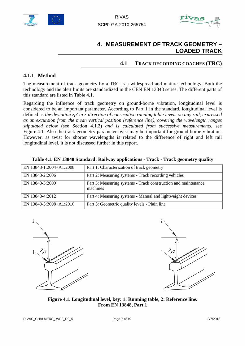
Regarding the influence of track geometry on ground-borne vibration, longitudinal level is considered to be an important parameter. According to Part 1 in the standard, longitudinal level is defined as the deviation zp' in z-direction of consecutive running table levels on any rail, expressed as an excursion from the mean vertical position (reference line), covering the wavelength ranges stipulated below (see Section 4.1.2) and is calculated from successive measurements, see Figure 4.1. Also the track geometry parameter twist may be important for ground-borne vibration. However, as twist for shorter wavelengths is related to the difference of right and left rail longitudinal level, it is not discussed further in this report.

Table 4.1. EN 13848 Standard: Railway applications - Track - Track geometry quality

EN 13848-1:2004+A1:2008 Part 1: Characterization of track geometry

EN 13848-2:2006 Part 2: Measuring systems - Track recording vehicles

EN 13848-3:2009 Part 3: Measuring systems - Track construction and maintenance machines

EN 13848-4:2012 Part 4: Measuring systems - Manual and lightweight devices

EN 13848-5:2008+A1:2010 Part 5: Geometric quality levels - Plain line

Figure 4.1. Longitudinal level, key: 1: Running table, 2: Reference line.

From EN 13848, Part 1

RIVAS

SCP0-GA-2010-265754


According to the standard, longitudinal level measurements shall either be made using an inertial system or by a versine system (that should preferably be asymmetric), or by a combination of both methods. If the versine method is used, an adjustment of the measured signals is necessary to eliminate the influence of the transfer function on the versine system. The measured value of the versine shall also be indicated in accordance with EN 13848-2.

It is also stipulated that the measurements should be performed under loaded conditions with a wheel load of at least 2.5 metric tonnes. This requirement means that the measured longitudinal level is a combination of vertical geometry irregularities and track stiffness irregularities.

A recent trend in track geometry measurements is the use of unattended systems. These systems are fully automated and could be mounted on e.g. a locomotive in normal operation. Data is transmitted to a data center where further processing is undertaken.

Brief descriptions of TRC operating in Switzerland, Sweden and the UK are presented in Sections 4.1.3.

4.1.2 Analysis

The standard EN 13848 stipulates three wavelength intervals for evaluation of track geometry:

- D1 (3 – 25 m)

- D2 (25 – 70 m)

- D3 (70 – 150 m)

To detect shorter wavelengths, it is noted in the standard that the lower boundary of D1 should be extended to 1 m. The D2 and D3 intervals are generally not relevant for ground vibration at normal vehicle speeds, see Table 3.1.

The maximum sampling distance is stipulated as 0.5 m but most TRC use a shorter sampling distance. Sampling distances down to 0.05 m are reported for some TRC, theoretically enabling evaluation of D1 from 0.1 m (practically from approximately 0.2 – 0.3 m). Nevertheless, Infrastructure Managers will generally refer to the standard EN 13848 and apply a low-pass filtering of data from 1 or 3 m. Thus, the D1 interval is maintained even though the actual sampling distance allows for an evaluation of shorter wavelengths.

Longitudinal level is a track geometry parameter. Misalignments of shorter wavelengths than 0.5 – 1 m are in most cases rail irregularities such as acoustic roughness, corrugation or a discontinuity in the rail caused by a weld or a joint. These short misalignments are generally not considered as track geometry misalignments.

However, for monitoring of loaded track geometry quality related to ground-borne vibration, it is noted here that using the already existing measurement range of TRC and thereby extending the range of measured wavelengths down to 0.2 m would cover most of the relevant wavelength range even at low train speeds.

According to the standard, the measurement accuracy of longitudinal level should be better than 1 mm for D1. Normally the reproducibility of the measurement system is tested by measuring the same track in both directions at different speeds. Reproducibility (95 % percentile) of 0.8 mm is required (D1). Reproducibility values for longitudinal level measured by modern TRC are reported in the range of 0.15 – 0.4 mm (D1), somewhat depending on the quality of track, the number of

RIVAS

SCP0-GA-2010-265754


curves and the measurement technology. These low values are extraordinary considering that the measurements are taken at speeds up to 300 km/h with a sampling distance of 5 – 50 cm.

Track geometry quality is monitored with intervals ranging from one measurement per year (tracks with low operation) to several measurements per week in the case of an unattended system.

The normal use and analysis of longitudinal level is to compare values with the standard to detect alert level exceedances. Standard deviation of longitudinal level evaluated over e.g. 200 metres is used to compare consecutive measurements and to plan maintenance based on degradation rate. Wavelength spectra are sometimes calculated, but this is more of a special analysis not used on a daily basis.

It is not a common procedure to consider longitudinal level in the investigation of ground-borne vibration, although the awareness of the link between the two is increasing. Currently, there are no standards or guidelines of acceptable levels for longitudinal level in order to limit ground-borne vibration. Part of the work within RIVAS WP2 investigates this area.

4.1.3 SBB (Switzerland)

The SBB track recording coach has an opto-inertial track geometry measurement system (MerMec), Laserail™. It is a non-contact track measuring system with GPS navigation and dual optical measurement boxes to measure, record and analyse the track geometry. The system, which is fully compliant with the EN 13848 international standard, offers highly accurate measurements at speeds up to 400 km/h (SBB: 120 km/h) with real time reports of exceedances of allowed geometry. The measurement is performed with six optical boxes and with a sampling distance of 0.25 m. The SBB TRC (axle load 16 tonnes) measures track gauge, cross level/cant, twist, alignment (D1 and D2), longitudinal level (D1 and D2), and curvature. Information about analysis of data, wavelength intervals and accuracy are summarised in Table 4.2.

Figure 4.2. SBB track recording coach

RIVAS

SCP0-GA-2010-265754


Table 4.2. Data for SBB track recording coach

Data-analysis

• 3D reconstruction of rail profiles from pictures

• For each rail, extraction of three level reference points based on 3D laser profiles at front, central and rear

Running mean over 25 m

D1 filtered signal: bandpass filter with 3 m < λ ≤ 25 m

D2 filtered signal: bandpass filter with 25 m < λ ≤ 70 m

Accuracy D1: < ± 1 mm

Standard EN-13848-1

4.1.4 Infranord (Sweden)

Infranord holds the current contract for track and overhead wire measurements in Sweden after procurement in 2009. Four different vehicles are used in the assignment, three IMV100 (Infranord Measurement Vehicle, maximum speed 100 km/h), see Figure 7.5, and one IMV200 (Infranord Measurement Vehicle, 200 km/h), see Figure 4.3. All four vehicles measure track geometry quality according to EN13848. Longitudinal level is measured with accelerometers mounted in the carbody and by compensation LVDTs (Linear Variable Differential Transformer) between axle and carbody. The three IMV100 are also equipped with a mechanical chord in order to measure longitudinal level and alignment in harsh weather conditions when lasers (for alignment) fail. This combination is the basis for the new stiffness measurement method EVS (EBER Vertical Stiffness) described in Section 7.1.4.

IMV200 also monitors overhead wire, both with and without contact, corrugation and rail profile.

IMV100 also monitors overhead wire (only without contact) and ballast profile.

All vehicles use a sampling distance of 0.05 m for track geometry quality. However, during post-processing, data are resampled to 0.25 m before delivering results to Trafikverket.

Figure 4.3. Swedish TRC IMV 200 in operation from March 2013

RIVAS

SCP0-GA-2010-265754


4.1.5 Network Rail (UK)

The Network Rail New Measurement Train (NMT) is a converted high-speed train consisting of Class 43 power cars (17.5 tonnes axle load) and Mark 3 coaches. It is used to monitor various aspects of track and OLE (Overhead Line Equipment) condition at 125 mph (201 km/h). Train positioning is achieved by a combination of an on-board GPS, odometry tachometers from a starting reference point, an inertial unit to know when the train has changed tracks and an underlying map, called the Network Rail Infrastructure Model (NRIM). Positional information has a general accuracy of 2 metres and a guaranteed accuracy of 16 metres.

The layout described in Figure 4.4 is typical for vertical profile measurements. On each side there is a displacement transducer between the bogie frame and the axle box. An inertial box containing a triaxial arrangement of accelerometers and rate gyroscopes is suspended from the bogie frame. The transducer signals are combined to create a reference path. Also suspended from the frame are optical scanners that locate the relative position of each rail. Combining the data from these scanners with the reference path gives the track geometry data. Other systems use LVDT transducers as well. Track geometry is measured according to the EN 13848 series.

Rail welds and insulation joints form small-scale irregularities on the rail surface generating a broad-band frequency content of the vertical wheel‒rail contact forces that may induce ground-borne vibration. Welding of the rail often results in a cusp- or dip-like discontinuity of the running surface. Rail joints are also characterized by a gap with a given width. In addition, there may be a difference in height (misalignment, gap height) between the two adjacent rail ends. The dip can be approximated by a quadratic function, for both rail joints and rail welds.

Information on dip angle for a loaded track may be computed from the NMT measurements of longitudinal level to detect broken rail, cracked fishplates and rail-end damage. It is important that data is measured at a sufficiently fine interval for twist and ramp angle to be fully determined. This means a sampling distance in the order of 250 mm. The dip angle is usually expressed in milliradian units. A separate dip angle signal is generated for left and right rails.

Figure 4.4. (left) NR Recording car, (right) Layout for the vertical track geometry measurement system

RIVAS

SCP0-GA-2010-265754


4.1.6 Examples of application

As one example of application with the SBB TRC, measurements of track geometry are presented for a track at Kiesen with and without Under Sleeper Pads (USP) [6].

Figure 4.5 shows the results of three measurements of track twist on SBB track 418 in 2005 and 2006. On track 418, there are two test sections with different USP (USP4 and USP5) and one reference section without USP. All measurements were performed after a track renewal. The green line is from September 2005, the blue line is from March 2006 and the pink line is from October 2006. Figure 4.6 shows the corresponding results of longitudinal level for the left rail of track 418. Especially the results of the twist measurements for both test tracks at Kiesen show that the sections with USP tend to result in a better track quality than the reference section without USP. The period was too short to observe the long term behaviour.

Figure 4.5. Results of track twist measurements on SBB track 418 at Kiesen

RIVAS

SCP0-GA-2010-265754


Figure 4.6. Results of longitudinal level measurements (left rail) on SBB track 418 at Kiesen

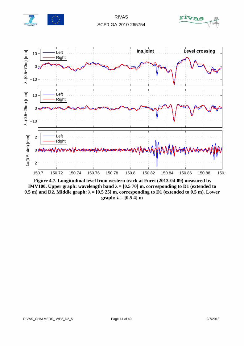
One example of longitudinal level over a distance of 200 m, measured by an IMV100, is shown in Figure 4.7. The test site is Furet in Sweden. Two larger faults can be observed. At km 150+829, there is an insulation joint on the left rail, and at km 150+848 there is a large fault at the start of a level crossing (the centre of the level crossing is marked at km 150+856 in the figure).

The results have been filtered to different wavelength bands. The top graph of Figure 4.7 is the combination of D1 and D2 (lower boundary extended to 0.5 m). The middle graph of the figure corresponds to D1 (lower boundary extended to 0.5 m), while the lower graph shows short defects between 0.5 and 4 metres of wavelength.

Considering the D1 interval, the magnitude of the fault at 150+848 is 11 mm. However when taking also the D2 interval into account, the fault magnitude is 14 mm. The fault at the insulation joint does not have a significant long-wavelength contribution, leading to an equal appearance between the top (D1+D2) and middle (D1) graphs. It can be observed from the lower graph that the insulation joint has a large short-wavelength contribution, possibly inducing high levels of wheel‒rail contact forces and ground-borne vibration.

RIVAS

SCP0-GA-2010-265754


−10

0

10

λ=(0

.5−

70m

) [m

m]

Ins.joint Level crossingLeft

Right

−10

0

10

λ=(0

.5−

25m

) [m

m]

LeftRight

150.7 150.72 150.74 150.76 150.78 150.8 150.82 150.84 150.86 150.88 150.9

−2

0

2

λ=(0

.5−

4m)

[mm

]

LeftRight

Figure 4.7. Longitudinal level from western track at Furet (2013-04-09) measured by IMV100. Upper graph: wavelength band λ = [0.5 70] m, corresponding to D1 (extended to

0.5 m) and D2. Middle graph: λ = [0.5 25] m, corresponding to D1 (extended to 0.5 m). Lower graph: λ = [0.5 4] m

RIVAS

SCP0-GA-2010-265754


4.2 CONTINUOUS TRACK MONITORING – CTM

Continuous track monitoring with regularly scheduled trains provides information on track geometry quality in short time intervals as a by-product of the train operation. This allows for

• Forecast of track defect development

• Verification of quality of repair

• Improvement of maintenance management

4.2.1 Method

The CTM measurement system used by DB is installed in the restaurant car of an ICE 2 high-speed train [7]. Since this train is used in regular service, a very robust setup was chosen and optical systems had to be excluded. The measurement system is based on acceleration measurements and has been in service since 2004. It consists of the components listed in Table 4.3.

Table 4.3. Components and applications of DB CTM measurement system

Points of Measurement: Signal processing:

Accelerometers on axle boxes (vertical and horizontal)

Assessment of track geometry (according to DB standard); track geometry of short wavelength (e.g. switches; rail welds)

Accelerometer on the bogie frame (horizontal) Assessment of running behaviour (according to DB standard)

Accelerometer inside the coach body Assessment of running behaviour and ride comfort (according to DB standard and UIC 513/prEN12299)

The accelerometers on the axle boxes are placed on the trailing wheelset of the first bogie (axle load 12 tonnes) and on the leading wheelset of the second bogie (axle load 14 tonnes). The maximum speed is 280 km/h, although the maximum operating speed is 250 km/h. In addition to the acceleration sensors, an inertial measurement unit (IMU, with six degrees of freedom) is installed to measure track alignment. The positioning is supported by a GPS system in the coach so that the measured signals can be assigned to the exact position of the track. An overview of the system is shown in Figure 4.8.

The measured raw data is transferred to a maintenance database on a weekly basis. The data for specific track segments, which are under special surveillance or must meet special criteria, are transferred on a daily basis. The operation of the system can be controlled remotely. The data processing is shown in Figure 4.9.

RIVAS

SCP0-GA-2010-265754


Figure 4.8. CTM installation on ICE 2 train

Figure 4.9. Data processing of CTM-installation on ICE 2 train

RIVAS

SCP0-GA-2010-265754


4.2.2 Analysis

The system measures the acceleration signals with a sampling frequency of 2 kHz. To obtain geometry data, the time-dependent signal is integrated twice and transformed into a signal of geometry at a sampling distance of 5 cm. Therefore wavelengths of track irregularities down to 0.3 m can be detected. The influence of variation in track dynamics on wheelset response is neglected at the time, but by considering the difference in axle loads (12 tonnes versus 14 tonnes) it could be included. The influence of vehicle speed has shown to be negligible within the usual speed range.

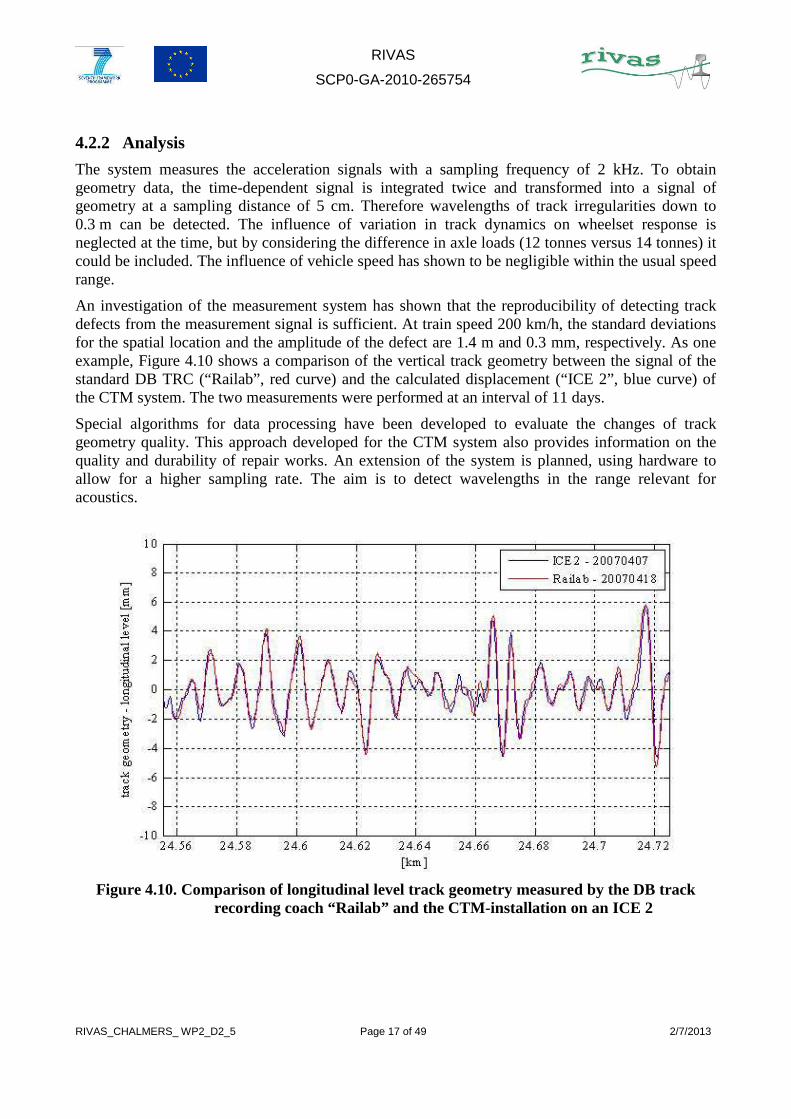
An investigation of the measurement system has shown that the reproducibility of detecting track defects from the measurement signal is sufficient. At train speed 200 km/h, the standard deviations for the spatial location and the amplitude of the defect are 1.4 m and 0.3 mm, respectively. As one example, Figure 4.10 shows a comparison of the vertical track geometry between the signal of the standard DB TRC (“Railab”, red curve) and the calculated displacement (“ICE 2”, blue curve) of the CTM system. The two measurements were performed at an interval of 11 days.

Special algorithms for data processing have been developed to evaluate the changes of track geometry quality. This approach developed for the CTM system also provides information on the quality and durability of repair works. An extension of the system is planned, using hardware to allow for a higher sampling rate. The aim is to detect wavelengths in the range relevant for acoustics.

Figure 4.10. Comparison of longitudinal level track geometry measured by the DB track recording coach “Railab” and the CTM-installation on an ICE 2

RIVAS

SCP0-GA-2010-265754



Inspection of geometry

The CTM system can be used for inspection of track geometry, in addition to the monitoring already performed by the standard DB TRC Railab. According to DB regulations, the inspection frequency for track geometry quality is determined by the permissible line speed vperm, varying between every 18 months (for vperm ≤ 80 km/h) and every 3 months (for vperm > 230 km/h). During an inspection of track geometry, the lateral and vertical deflections of both rails, the cant, the track gauge and the track twist are measured. The sampling distance of these values is independent of the speed of the recording vehicle.

Measurement of vehicle reaction

In contrast to the inspection of track geometry, the measurement of vehicle reactions is dependent of vehicle speed. These measurements are conducted on lines where vperm > 160 km/h and on lines where tilting trains are operating. With this type of measurement, the dynamic vehicle‒track interaction is assessed. The forces between wheel and rail, the lateral acceleration of the bogie and the vertical acceleration of the car body are recorded. During the measurement campaign the vehicle has to run with the permissible speed of the line. The assessment limits are derived from the UIC leaflet 518.

Tests have shown a good correlation between track geometry quality and vehicle reaction in the car body. In Figure 4.11, the standard deviation of the vertical track quality (blue curve) and the running behaviour of the vehicle (red curve) are displayed, showing a high degree of correlation.

Figure 4.11. Correlation between track geometry and running behaviour

RIVAS

SCP0-GA-2010-265754


Tracing of development of track defects, forecast

The following requirements are decisive for tracing the development and enabling a forecast of track defects:

• The observed track section has to be measured in short time intervals • The measurement results have to be accurate and reproducible • A track defect has to be located precisely in order to process the obtained data automatically

Two examples are given to demonstrate the tracing of track defects for the assessment of the sustainability of corrective maintenance. The effect of maintenance on three adjacent track defects is shown in Figure 4.12. The graph illustrates the vertical track geometry quality (in mm) depending on spatial location (x-axis) and time (y-axis). On the right hand side of the graph, the colour bar represents the size of the track defect. In the upper part of the graph, three adjacent track defects are located between km 135.82 and 135.84. In May 2007, the track was tamped (reducing the red regions in Figure 4.12). The tamping was carried out properly, as can be observed in the graph since track quality remains at a high level from May 2007 until February 2008.

Figure 4.13 shows a track defect that was badly corrected. At km 136.123, a vertical track defect can be noticed. The size of the track defect is 12 mm. In the first week of July the track defect was tamped locally. In contrast to the example above, in the next six months the track defect increased to its original size. The rapid growth of the defect gives an indication on the choice of the maintenance measure and the quality of the maintenance work.

Figure 4.12. Development of track quality after a maintenance operation with good durability

RIVAS

SCP0-GA-2010-265754


Figure 4.13. Development of track quality after a maintenance operation with poor durability

RIVAS

SCP0-GA-2010-265754


5. MEASUREMENT OF TRACK GEOMETRY – NON-LOADED TRACK

5.1 DISPLACEMENT TRANSDUCERS AND

ACCELEROMETER -BASED TROLLEYS

Non-loaded track geometry and local track defects can be measured using trolley-based measurement systems. Although the trolleys are designed for measuring rail roughness/corrugation, they can also be used to measure local defects.

5.1.1 Method

Two principles exist to measure non-loaded geometry: measurement using displacement sensors and measurement using accelerometers.

In the case of measurement using displacement sensors, the vertical displacement is measured with respect to a reference beam mounted on the rail (displacement transducers running on a stationary straight-edge). This reference beam, with a length of in general about 1 m, can be either fixed at a specific location (discrete measurement) or can be moved along the rail using the trolley for a continuous measurement of rail geometry. In the case of measurement using an accelerometer, the vertical displacement is basically determined by double integration of the acceleration signal that is measured when pushing the trolley along the rail surface.

In both cases, the position along the rail is recorded simultaneously, such that the result is a measure of the vertical rail irregularity as a function of the position along the rail.

Table 5.1 provides an overview of existing measurement devices. The table is not complete and it does not include vehicle mounted devices.

Table 5.1. Overview of existing measurement systems

Instrument Measurement principle

Discrete/continuous

APT – RSA Displacement Continuous

Müller-BBM – M|Rail Displacement Discrete

Lloyd’s Register ODS Displacement Discrete

RailMeasurement – CAT Acceleration Continuous

RIVAS

SCP0-GA-2010-265754


Figure 5.1 shows the APT-RSA (Rail Surface Analyser) used to measure rail roughness and the geometry of local defects during a RIVAS measurement campaign in Switzerland (see RIVAS deliverable D2.1). The figure on the left shows the trolley mounted on the track. The figure on the right shows the bottom of the device with the three measurement probes that are pushed against the rail surface. These measurement probes are connected to LVDT transducers.

Figure 5.2 shows the CAT (Corrugation Analysis Trolley) by RailMeasurement Ltd. The figure on the left shows the trolley mounted on the track. The figure on the right shows a more detailed view of the device. The sampling distance is 1 mm (or 2 mm) and the precision of displacement measurement is 0.01 µm [8,9].

Trolley-based measurement systems have the advantage that they can be applied very easily due to their mobility and without the need of a dedicated measurement train. At the same time, this advantage is also a drawback for measurements of local defects since it is the unloaded geometry that is measured.

Figure 5.1. Example of trolley (APT-RSA) based on displacement transducers

Figure 5.2. Example of trolley (CAT) based on acceleration measurements. From [8]

RIVAS

SCP0-GA-2010-265754


5.1.2 Analysis

Figure 5.2 shows the result of a rail roughness measurement using the APT-RSA system performed in Goldau–Steinen, Switzerland.

(a)

RIVAS

SCP0-GA-2010-265754


(b)

Figure 5.2. Analysis of rail roughness measurement based on APT-RSA

Figure 5.2(a) shows

• Top: the measured displacement (middle transducer) as a function of position along the rail. The sampling distance is dependent on the system, in this case it is 1 mm. The measurement noise floor of the displacement measurements is 0.1 µm.

• Middle: the displacement spectrum in the wavelength range between 0.31 cm and 50 cm. The lower wavelength boundary is determined by the sampling distance, while the higher wavelength boundary is determined by the length of the measurement device. The spectrum is compared to the IS0 3095 limit spectrum.

• Bottom: the spectrum as a function of position along the rail.

Figure 5.2(b) shows

• Top: the measured global amplitude (RMS) in the wavelength band between 0.4 cm and 50 cm for each of the transducers as a function of distance along the rail.

• Bottom: the displacement spectrum for each transducer.

RIVAS

SCP0-GA-2010-265754



The APT-RSA system has been used to measure several types of local track defect.

Figure 5.2 (see above) shows an example of a measurement with corrugation with wavelengths between 12.5 cm and 20 cm.

Figure 5.3 shows a measurement of rail irregularity at insulation joints and welds. The effects of both welds (green ellipses) and insulation joints (red ellipses) are clearly visible in the displacement measurements. Figure 5.4 shows a detailed measurement of an insulation joint. Figure 5.5 shows a similar measurement of a bad weld.

Figure 5.3. Measurement of welds (green ellipses) and insulation joints (red ellipses) using an APT-RSA

RIVAS

SCP0-GA-2010-265754


22 22.5 23 23.5

-600

-400

-200

0

200

distance(m)

D1(

+10m

m)

( µm)

22 22.5 23 23.5

-600

-400

-200

0

200

distance(m)

D2(

cent

er)

( µm

)

22 22.5 23 23.5

-600

-400

-200

0

200

distance(m)

D3(

-10m

m)

( µm)

Figure 5.4. Detailed measurement of an insulation joint using an APT-RSA

Traffic

RIVAS

SCP0-GA-2010-265754


40 40.5 41 41.5 42 42.5

-800

-600

-400

-200

0

200

distance(m)

D1(

+10m

m)

( µm)

\\D2s-server\01_D2SINT\D1391_EC-UIC_RIVAS\05_Measurements\RAWdata\20111114-18_D2S_Sw itserland\S4_Schw yz_Bad_w eld\RSA\\ sq299_rec15.dat S4 - Schw yz

40 40.5 41 41.5 42 42.5

-800

-600

-400

-200

0

200

distance(m)

D2(

cent

er)

( µm

)


40 40.5 41 41.5 42 42.5

-800

-600

-400

-200

0

200

distance(m)

D3(

-10m

m)

( µm)


Figure 5.5. Detailed measurement of a poor weld using an APT-RSA

Traffic

RIVAS

SCP0-GA-2010-265754


5.2 VEHICLE MOUNTED INSTRUMENTS

The rail corrugation system RCS (developed by Mermec), see Figure 5.6, used by SBB and mounted on their TRC measures rail roughness/corrugation and summarises the results in windows of 25 cm. Based on bandpass filtering, the rail roughness is analysed in three wavelength bands ranging from short wavelengths (20 – 100 mm), (100 – 300 mm) to longer wavelengths (300 – 1000 mm). The system uses optical measurements of rail surface profile by recording surface irregularities with cameras and lasers through the Versine transfer function.

Figure 5.7 illustrates an example of results from a rail roughness measurement at Lengnau-Pieterlen. From top to bottom, the graphs show (sampled at every 25 cm and for right and left rails) the short wavelength (20 – 100 mm) bandpass filtered result, then the midrange (100 – 300 mm) filtered data and at the bottom the long wavelength (300 – 1000 mm) filtered data. The yellow band shows acceptable values for corrugation adapted for each bandpass range.

Figure 5.6. Principle sketch of RCS system to measure rail roughness

RIVAS

SCP0-GA-2010-265754


Figure 5.7. Rail roughness measurements based on RCS at Lengnau-Pieterlen by SBB TRC 19.11.2012

The Rail Corrugation Analyser (RCA) developed by RailMeasurement Ltd, see Figure 5.8, is typically mounted on the chassis of a reprofiling train to determine if rail irregularities (corrugation, roughness) have been brought within acceptable limits. In current applications, the vertical load on each wheel is up to 1 kN. Based on comparisons with the CAT, the RCA provides accurate measurements of vertical rail irregularities in the wavelength interval 0.02 – 5 m, even at vehicle speeds up to 50 km/h, see Figure 5.9. Measured irregularity levels at shorter wavelengths than 0.02 m are lower with the RCA than with the CAT because of the larger diameter of the measurement wheel (the diameter of the measurement wheel is about 0.23 m). The accuracy of the RCA (when compared to the CAT) is 2 µm when evaluated as a RMS in the wavelength band 100 – 300 mm.

The RCA uses accelerometers and an inertial system to measure irregularities at a sampling distance of 2 mm. The precision of displacement measurement is 0.1 µm [8].

RIVAS

SCP0-GA-2010-265754


Figure 5.8. Rail Corrugation Analyser RCA. From [8]

Figure 5.9. Illustration of reproducibility of the RCA, and a validation of the RCA versus measurement with a CAT. From [10]

RIVAS

SCP0-GA-2010-265754


6. COMBINATION OF TRACK IRREGULARITY SPECTRA MEASURED BY DIFFERENT SYSTEMS

Vertical irregularities experienced by a vehicle origin from geometrical irregularities on the rail, from variations in the unloaded level of the foundation supporting the track superstructure, and from variations in stiffness of pads, sleepers, ballast and soil. The former is most often characterized by the presence of rail roughness or corrugation, but it could also be a local defect such as a weld, joint or insulation joint. The other two contributions to the total vertical irregularity are most often characterized by the measurement of longitudinal level for a loaded track (i.e. the combined effect of these two contributions).

Rail roughness is commonly measured and assessed within the wavelength band 0.5 – 31.5 cm [11]. The upper boundary is sometimes extended to sleeper distance and sometimes even higher.

Longitudinal level is measured according to the standard EN 13848, see Section 4. The lowest band D1 covers the wavelength interval 3 – 25 m, possibly extended down to 1 m. Thus, there is generally a gap between approximately the wavelengths 0.5 m and 3 m where accurate information about vertical track irregularities is missing. As these wavelengths excite frequencies important for ground vibration, see Table 3.1, there is a need for an approach to close this gap.

Figure 6.1 illustrates an example of combining the results (narrow band spectra of power spectral density) from two different measurement systems [12]. In this case, a CAT was used to measure rail roughness (unloaded track) in the wavelength band 0.01 – 1.0 m, while a TRC measured longitudinal level (loaded track) for wavelengths between 0.6 m and 100 m. From this example, it seems possible to interpolate between the two spectra as well as to estimate an overall linear (on a logarithmic scale) trend in the complete wavelength interval 0.01 – 100 m. Here, it was found that the slope of the dashed line in Figure 6.1 is λ

2.85, where λ is the irregularity wavelength.

In another study [13], where the aim was to validate a model for prediction of ground-borne vibration versus field measurements, the same two types of measurement system were used to determine the vertical track irregularity. The short wavelength range was measured by a CAT. Here, it was found to be possible to extract reliable data from the trolley for wavelengths even up to 3 m. Irregularities with longer wavelengths were obtained from routine measurements by a TRC. Two test sites were investigated using two different TRCs. At one site, the TRC measurements were filtered with a cut-off wavelength at 1 m, whereas at the other site the cut-off wavelength was 3 m. The combined spectra for the two sites are shown in Figure 6.2. It is observed that the two measurement methods generate spectra that to a significant extent are consistent with one another.

Referring to these two studies reported in [12,13], it is concluded by Grassie [4] that the one-third octave spectra measured by the TRC and the CAT correlate well in the wavelength interval around 1 – 3 m which is the upper limit of wavelength measurable with the CAT and the lower limit with the TRC.

The most straightforward approach to close the gap, 0.5 m – 3 m, is to extend the D1 waveband down to 0.5 m, by reducing the sampling distance of the TRC (increasing the sample rate). If the measurement system of longitudinal level includes a sensor (e.g. accelerometer) mounted in a position with large structural vibration (e.g. on the wheelset), extra care needs to be taken to compensate for this. A high-speed TRC will experience axle and wheel resonances, sometimes starting as low as 50-100 Hz. This may disturb the measurements. A laser system mounted on the carbody using an inertial platform to compensate for carbody movements will be better suited if

RIVAS

SCP0-GA-2010-265754


axle/wheel resonances are a problem. Another alternative is to extend the roughness measurements (by using e.g. the RCS or CAT described in Section 5) up to 1 m or 3 m.

100 10 1 0.1 0.01

10−5

100

Wavelength [ m ]

PS

D o

f ver

tical

rai

l and

trac

k ge

omet

ry [

mm

2 *m ]

Measurements with CAT →

← Measurements with TRC

Normal trackGood track EN 3095

Figure 6.1. Example of combined power spectral density of longitudinal level and rail

roughness. Rail geometry quality measured with CAT (Corrugation Analysis Trolley) and track geometry quality measured with inertial TRC. From [12]

RIVAS

SCP0-GA-2010-265754


Figure 6.2. Irregularity spectra in one-third octave bands from two different sites. The

irregularities were measured by a CAT trolley (solid lines) and a TRC (dashed lines). From [13]

RIVAS

SCP0-GA-2010-265754


7. MEASUREMENT OF TRACK STIFFNESS – LOADED TRACK

Measurement of stiffness along a railway track is a relatively new technology. Test and research measurements have been carried out in some countries during the last two decades. The measurement technology has now begun to mature and is commercially available. Track stiffness measurement has applications in the fields of:

- Track maintenance

o Indicator of root cause for track irregularities at problem sites

o Evaluation of transition zones

o Soft soil detection

o Voided sleepers detection

o Rail bending / rail crack propagation

o Vibration

- Upgrading of track for higher axle load and/or speed

- Verification of newly built tracks

The RIVAS project focuses on the influence of track stiffness variation on ground vibration, which has not been thoroughly investigated in previous studies. Certainly, soft soils have been studied thoroughly regarding vibration. Different aspects related to track stiffness and ground vibration are listed in Table 7.1.

Table 7.1. Aspects of track stiffness, and relation to ground vibration

Soft soil Low track stiffness is often an indicator of soft soil. Soft soils are prone for vibration propagation

Track stiffness variation

Variation of track stiffness in the upper (ballast, subballast) or lower (material fill, soil) layers along the track will generate dynamic wheel‒rail contact forces during a train passage, possibly inducing vibration

Transition zones Transition zones often come with variable track stiffness, e.g. at bridge approaches. These will often increase the excitation of dynamic wheel‒rail contact forces. Also track geometry degradation is common which will further increase forces

Hanging sleepers If there is a gap between sleeper and ballast, the gap will close during a wheel passage, possibly inducing a load impulse to the ground. This is believed to be an important excitation mechanism for vibration

RIVAS

SCP0-GA-2010-265754


7.1.1 Method

There are a couple of different methods to measure track stiffness. If two or more methods are compared for the same track, the recorded vertical track stiffnesses will probably not match exactly. Some of the circumstances that might lead to different results are listed below:

• Static preload: Different static preloads on the measurement wheelset will most probably result in different stiffness values. Some methods also use a reference preload (lightly load axle, or non-loaded track). Depending on the selected load, the first part of the force/deflection curve (where gaps between sleeper and ballast will close) may or may not be possible to detect.

• Excitation frequency and vehicle speed: The measurement principle used on the Infranord RSMV (Rolling Stiffness Measurement Vehicle, see below) uses a prescribed dynamic excitation, but also the methods that use a rolling wheelset as excitation will excite the track with a frequency content determined by the irregularities in track geometry and stiffness. If the speed of the measurement vehicle is increased, so will the frequency content. Since the dynamic track stiffness is not constant with frequency, the result may differ.

• Spatial resolution: The different measurement principles may have different spatial resolutions.

• Model dependency: Some of the measurement principles measure the deflection of the rail some distance away from the exciting wheelset. To calculate the rail deflection under the wheelset, a beam model for the rail bending has to be used. The beam models are for example according to Winkler or Zimmermann and can introduce an uncertainty.

• Degree of influence from track irregularities: Track irregularities, especially longitudinal level, may disturb the stiffness measurements since the displacement transducers in most cases will measure a combination of deflection due to track flexibility and displacement due to track irregularities. Wheel out-of-roundness and wheel flats will introduce the same kind of disturbance.

A compilation of available methods is given in [14]. Examples of methods are presented in the sections below.

RIVAS

SCP0-GA-2010-265754


7.1.2 SBB Track deflection measurement wagon

Using the deflection measurement wagon developed by SBB (see Figure 7.1), a continuous monitoring of track deflections can be performed at vehicle speeds in the range 10 – 15 km/h. The measurement method consists in measuring the relative track deflection between an unloaded wagon (due to the very low axle load, the track deflection generated by this wagon can be taken as negligible) and a loaded axle (20 tonnes). The instrumentation includes an incremental sensor Heidenhain LS 220 and a PC digital display unit IK 121.

To obtain a deflection curve which is interpretable, normally a low pass filter with cut-off wavelength in the interval 10 m – 20 m is applied. The measurement accuracy is about ± 0.2 mm. To improve the accuracy, normally the deflection measurement is repeated but this time with both wagons unloaded. Then the unloaded deflection measurement is subtracted from the loaded deflection measurement. The sampling distance is around 5 cm.

The measurements are normally not used to detect hanging sleepers, but longer wavelength disturbances caused by variations of soil properties, at bridges, and the influence of USP, etc, are investigated. Nevertheless a severely hanging sleeper could be detected if the measured deflection is high even when the low pass filter is applied. The reason to apply the low pass filter for every measurement is that low levels of wheel out-of-roundness significantly influence the measurements and these effects have to be eliminated for the interpretation of the measured curves.

Figure 7.1. SBB track deflection measurement wagon, axle load 20 metric tonnes

RIVAS

SCP0-GA-2010-265754


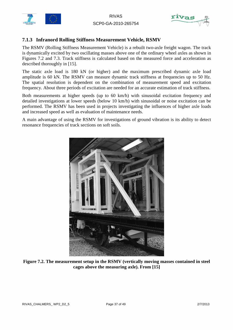
7.1.3 Infranord Rolling Stiffness Measurement Vehicle, RSMV

The RSMV (Rolling Stiffness Measurement Vehicle) is a rebuilt two-axle freight wagon. The track is dynamically excited by two oscillating masses above one of the ordinary wheel axles as shown in Figures 7.2 and 7.3. Track stiffness is calculated based on the measured force and acceleration as described thoroughly in [15].

The static axle load is 180 kN (or higher) and the maximum prescribed dynamic axle load amplitude is 60 kN. The RSMV can measure dynamic track stiffness at frequencies up to 50 Hz. The spatial resolution is dependent on the combination of measurement speed and excitation frequency. About three periods of excitation are needed for an accurate estimation of track stiffness.

Both measurements at higher speeds (up to 60 km/h) with sinusoidal excitation frequency and detailed investigations at lower speeds (below 10 km/h) with sinusoidal or noise excitation can be performed. The RSMV has been used in projects investigating the influences of higher axle loads and increased speed as well as evaluation of maintenance needs.

A main advantage of using the RSMV for investigations of ground vibration is its ability to detect resonance frequencies of track sections on soft soils.

Figure 7.2. The measurement setup in the RSMV (vertically moving masses contained in steel cages above the measuring axle). From [15]

RIVAS

SCP0-GA-2010-265754


Figure 7.3. Measurement principle (one side only) of RSMV. From [15]

7.1.4 EBER Vertical Stiffness, EVS

The EVS-method (EBER Vertical Stiffness) [16] is based on the fact that a longitudinal level measurement of a track being subjected to a loaded axle comprises two parts. The two parts are illustrated in part A of Figure 7.4. The first part relates to level variations due to irregularities present in the unloaded track (non-loaded track geometry, blue solid line), while the second part relates to the extra deflection which is due to the loaded axle (black dashed-dotted line). According to standards and common practice, measurement of level sIn(x) at position x should always be for a loaded track sL(x), illustrated by the red dashed line in the figure. Thus, the measured level from a track recording coach consists of two parts, the unloaded track geometry sU(x) and the deflection due to the loading w(x,x1). This can be expressed as

),()()()( 1ULIn xxwxsxsxs +== (1)

The double indexing of w(x,x1) means that the deflection at position x is caused by a load applied at x1. Note that sL could also be written with a double index for completeness, but this is omitted in the following meaning that x1 = x.

Level can also be measured using a chord/versine method. Figure 7.4, part B, shows an example of track deflection where the loaded measurement wheel (C2) is placed in the middle and the outer (possibly lightly loaded) measurement wheels (C1, C3) are placed at distances –b and +a from the middle wheel. Level readings from a chord system are taken as the difference between the C1-C3 chord and C2, as illustrated in the figure.

The mathematical description of a chord level system is

(2)

where the three reference points of the versine measuring system are at the positions x-b, x and x+a and where l = a+b.

RIVAS

SCP0-GA-2010-265754


−6

−4

−2

0

2

4

Leve

l [m

m]

A)

x

w, s

Unloaded level, sU

Loaded level, sL

Deflection, w(x,x)

−10 −8 −6 −4 −2 0 2 4 6 8 10

−2

0

2

4

6

Leve

l [m

m]

b a

C1

C2 C3

Q

↓B)

Unloaded level, sU

Loaded level one axle, sL

Deflection one axle, w(x,0)

Figure 7.4. Example of track deflection for unloaded and loaded track (A), and the effect of a single wheel load combined with a chord measurement (B)

The inertial and chord based systems have existed side by side for many years. Some focus has been put on generating good transfer functions in order to make the measurements comparable. The inventive step in this method is to compare the two systems with the goal to separate the unloaded track geometry and the loaded track geometry as in part A of the figure. Based on this approach, both track deflection and track stiffness can be determined.

The chord function according to Eq. (2) assumes that the outer points have the same loading condition as the middle point. If a proper deduction is made, with the same notation as in Eq. (1), the chord measurement result is given as

lxbxwbxsaxaxwaxsbxxws

lxbxwbxsaxaxwaxsbxsxs

/)),()(()),()(((),(

/)),()(()),()((()()(

UUU

UULC

−+−++++−+==−+−++++−=

(3)

This is illustrated in Figure 7.4, part B where C1 and C3 are running on nearly non-loaded track.

In order to compare the measurements from the inertia based system and the chord system, the level measurements of the inertia based system are converted to the same reference system as the chord system by substituting Eq. (1) into Eq. (2) such that

RIVAS

SCP0-GA-2010-265754


lbxbxawaxaxbwxxw

lbxasaxbsxsxs

/)),(),((),(

/))()(()()( UUUC_I

−−+++−

+−++−= (4)

This could be illustrated in Figure 7.4, part A, if the same chord illustration as in part B was drawn on the loaded level (red dashed line), as both C2 and C1, C3 are fully loaded.

By taking the difference between the chord measurement, Eq. (3), and the filtered inertial measurements, Eq. (4), a result cleared from unloaded level is obtained as

lbxbxwxbxwaaxaxwxaxwb

xsxs

/))),(),(()),(),(((

)()( CC_I

−−−−+++−+=

=− (5)

The contribution to the measured level originating from unloaded irregularities of the railway track is thereby eliminated. By measuring or simulating the wheel‒rail contact force, the loaded track stiffness can also be determined.

This approach has been implemented on the Infranord vehicle IMV100 shown in Figure 7.5. The axle load of each measurement wheel is 100 kg.

Figure 7.5. Track geometry recording coach IMV100, also capable of measuring track stiffness based on the EVS method

7.1.5 TTCI

The TTCI (Transportation Technology Center in Pueblo, CO) method uses two differently loaded axles, as for the SBB method, to distinguish between longitudinal level and track deflection.

RIVAS

SCP0-GA-2010-265754


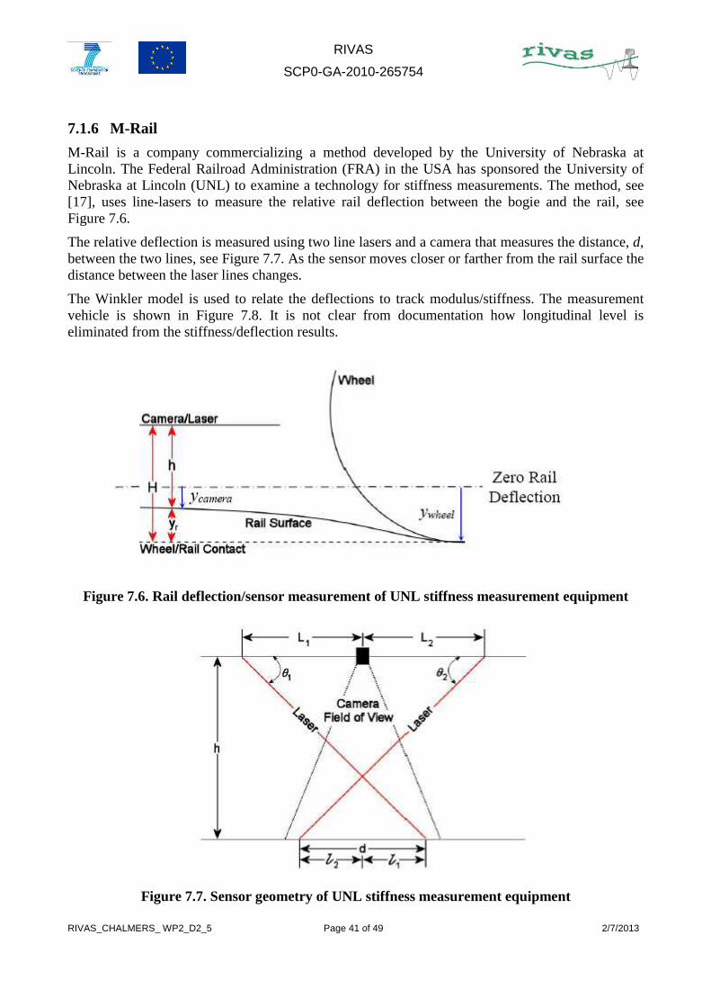
7.1.6 M-Rail

M-Rail is a company commercializing a method developed by the University of Nebraska at Lincoln. The Federal Railroad Administration (FRA) in the USA has sponsored the University of Nebraska at Lincoln (UNL) to examine a technology for stiffness measurements. The method, see [17], uses line-lasers to measure the relative rail deflection between the bogie and the rail, see Figure 7.6.

The relative deflection is measured using two line lasers and a camera that measures the distance, d, between the two lines, see Figure 7.7. As the sensor moves closer or farther from the rail surface the distance between the laser lines changes.

The Winkler model is used to relate the deflections to track modulus/stiffness. The measurement vehicle is shown in Figure 7.8. It is not clear from documentation how longitudinal level is eliminated from the stiffness/deflection results.

Figure 7.6. Rail deflection/sensor measurement of UNL stiffness measurement equipment

Figure 7.7. Sensor geometry of UNL stiffness measurement equipment

RIVAS

SCP0-GA-2010-265754


Figure 7.8. Measurement vehicle developed by M-Rail

7.1.7 Analysis

Methods to measure track stiffness and track deflection differ, and so does the processing, which is partly described above. Accuracy investigations are not available for all methods. The RSMV has a reported repeatability of 3.3 kN/mm (one standard deviation) [15].

The vehicles from TTCI, SBB and RSMV operate at low speeds (less than 50 km/h). The methods M-Rail and EVS can measure at nominal track speed.

Regarding ease of operation, TTCI, SBB and RSMV require a special measurement car. M-Rail can be fitted to any car. EVS is preferably fitted to a track recording coach to make use of the already existing systems for measurement of longitudinal level, but could also be fitted to any car.

The RSMV has the ability to analyse stiffness at different frequencies up to 50 Hz as it is a dynamic measurement with oscillating masses. All other methods monitor the displacement of an ordinary axle and cannot analyse stiffness at different frequencies.

For geotechnical monitoring, there is no need for frequent monitoring except if there are places with freezing/thawing or varying drainage. One measurement is sufficient to determine the conditions of the soft/stiff soil. For stiffness and displacement variations at shorter wavelengths which vary more with time, there is a need for more frequent measurements.

RIVAS

SCP0-GA-2010-265754



Figure 7.9 illustrates results from vertical deflection measurements of track 418 using the SBB track deflection monitoring car in 2006. As discussed previously in this report, track 418 contains two test sections with USP and one reference section without USP. The light grey line is from a measurement in January 2005 before the renewal of the track. The two other lines are from measurements after the renewal. The red line is from June 2006 and the blue line is from December 2006.

The vertical deflection measurements provide detailed information of the track deflection under load. The imperfections in the track (bad subsoil, underground passages etc.) can be clearly seen. In general, the sections with USP demonstrate a more homogeneous behaviour than the reference section without USP. At the transition zone between USP4 and USP5, a shift in vertical track deflection from about 0.8 mm to 1.6 mm can be observed due to the different stiffnesses of the USP materials.

Figure 7.9. Results of the vertical deflection measurements of track 418 at Kiesen

Figure 7.10 illustrates track deflection measured by the EVS-method at Furet in Sweden. The example is related to Figure 4.7 previously discussed for longitudinal level, see Section 4.1.6. The upper graph shows the full (unfiltered) track deflection, including the static mean deflection of 2 mm. The middle graph is filtered between 1 – 25 m, corresponding to the wavelength interval D1 used for longitudinal level. The upper and middle graphs are the same, except the mean static deflection present in the upper graph. The lower graph of Figure 7.10 shows the very short wavelength variations.

The large variations at the insulation joint and around the level crossing are also consequences of bad ballast support / hanging sleepers, which is easily detected with the method.

RIVAS

SCP0-GA-2010-265754


−6

−4

−2

0

λ=(1

−∞

) [m

m]

Ins.joint Level crossingLeft

Right

−2

0

2

λ=(1

−25

m)

[mm

]

LeftRight

150.7 150.72 150.74 150.76 150.78 150.8 150.82 150.84 150.86 150.88 150.9

−2

0

2

λ=(1

−4m

) [m

m]

LeftRight

Figure 7.10. Track deflection from western track at Furet (2013-04-09). Upper graph λ = [1 - ∞] m. Middle graph λ = [1 25] m, Lower graph λ = [0.5 4] m

Statistics of track stiffness over longer track sections with the RSMV are illustrated in Figure 7.11 [18]. Track 1 (50 kg rails and wooden sleepers) between Falun and Borlänge (24 km) carries mixed traffic with up to 25 tonnes axle load. Track 2 between Alvesta and Hässleholm (93 km) is a part of the southern main line carrying both freight traffic with up to 22.5 tonnes axle load and passenger traffic up to 200 km/h maximum speed. This track is mainly built of concrete sleepers with a mix of soft and stiff pads and 50/60 kg rails, although a smaller portion of wooden sleepers is also present. Finally Track 3 (concrete sleepers, soft pads and 60 kg rails) between Varberg and Gothenburg (48 km) on the western main line carries the same type of traffic as Track 2.

As can be seen from the upper part of Figure 7.11, stiffness magnitude can vary considerably between different tracks. Track 1 built with wooden sleepers and 50 kg rail evince distinct lower values of stiffness as compared with the other two tracks. The substructure of Track 1 is generally in good condition (mostly moraine). When stiffness phase is considered, Track 3 differs from the others as shown in the lower part of Figure 7.11. At this track, there are portions of soft clay along the track, which in most cases are reinforced with lime-cement columns. When dynamically excited, clay substructure appears with large stiffness phase delays at low frequencies.

RIVAS

SCP0-GA-2010-265754


0 50 100 150 2000

0.2

0.4

0.6

0.8

1

Stiffness magnitude [ kN/mm ]

dist

rubu

tion

−80 −60 −40 −20 00

0.2

0.4

0.6

0.8

1

Stiffness phase [ degrees ]

Cum

ulat

ive

Track 1Track 2Track 3

Figure 7.11. Cumulative distribution of dynamic track stiffness (at 11.4Hz) for three different tracks. From [18]

RIVAS

SCP0-GA-2010-265754


8. DISCUSSION

The dynamic component of vertical wheel–rail contact forces, as generated by irregularities in track geometry (longitudinal level, isolated defects, insulated joints, rail corrugation, switches & crossings, etc) and track stiffness (transition zones, hanging sleepers, culverts, etc), is an important source to ground-borne vibration and ground-borne noise. The overall objectives of RIVAS WP2 are to define, optimize and demonstrate different measures related to track and rolling stock maintenance to reduce excitation of ground-borne vibration at source.

One important aspect of controlling vibration levels is the availability of systems that accurately measure and monitor vertical track irregularities. Such systems have been surveyed in this report, covering methods measuring either unloaded or loaded track irregularities in the wavelength interval relevant for ground-borne vibration. A summary of important features of the different systems discussed in this report is listed in Table 8.1.

Unfortunately, none of the available systems measures the complete wavelength interval relevant for ground-borne vibration and ground-borne noise. For example at a conventional freight train speed of 80 km/h, the relevant wavelengths are from around 0.1 m up to about 10 m. In common practice and according to existing standards, TRC are used to assess loaded track geometry (longitudinal level) with wavelengths down to 3 m (sometimes 1 m), whereas hand-held accelerometer-based trolleys and mechanical displacement probes measure unloaded rail irregularities up to about 0.5 m. Thus, to cover the complete wavelength interval, a combination of measurement methods is required.

To improve the monitoring of longitudinal level at wavelengths important for ground-borne vibration and noise, it is suggested to introduce a new wavelength band (here it is referred to as D0, c.f. the EN standard 13848) containing wavelengths in the interval 0.5 – 3 m. Together, the D0 and D1 bands correspond to excitation frequencies in the range 0.9 – 44 Hz at vehicle speed 80 km/h (2 – 110 Hz at 200 km/h). Many existing TRC have the capability (sampling distance and accuracy) required to measure wavelengths down to 0.5 m but commonly a filtering of data is applied as information for the shorter wavelengths is currently not requested by existing standards. One important benefit of TRC is that the measured longitudinal level is a combination of contributions from irregularities in track geometry and track stiffness.

Rail irregularities with shorter wavelengths need to be measured by an accelerometer-based trolley, or preferably by equipment such as the Rail Corrugation Analyser or a laser system mounted on the carbody of a TRC (or similar) to cover larger portions of the network. Successful work where irregularity spectra (loaded and unloaded geometry) from two different measurement systems have been combined was discussed and illustrated in Section 6.

RIVAS

SCP0-GA-2010-265754


Table 8.1. Features of different systems for measurement of longitudinal level, rail irregularities and track stiffness

Type of irregularity

Axle load [tonnes]

Sampling distance [m]

Speed [km/h]

TRC – SBB Longitudinal level

16 0.25 120

TRC – IMV100 Longitudinal level

13 0.05 100

TRC – IMV200 Longitudinal level

12.7 0.05 200

TRC – NMT Longitudinal level and rail irregularities

17.5 0.25 200

CTM – DB Longitudinal level and rail irregularities

12/14 0.05 250

M|Rail - Müller-BBM

Rail irregularities 0 0.001 0

Lloyd’s Register ODS

Rail irregularities 0 0.001 0

RSA – APT Rail irregularities 0 0.001 1 m/s

CAT – RailMeasurement

Rail irregularities 0 0.001 1 m/s

RCA – RailMeasurement

Rail irregularities 0.2 0.002 50

RCS – Mermec Rail irregularities 0 0.25 120

Track deflection – SBB

Track stiffness 20 0.05 10 – 15

RSMV – Infranord

Track stiffness 18 0.05 ≤ 50

EVS – Infranord Track stiffness 13 / 0.2 0.05 100

RIVAS

SCP0-GA-2010-265754


9. REFERENCES

[1] RENVIB II Phase 1 – UIC Railway Vibration Project, State of the Art Review. J G Walker, G S Paddan and M J Griffin, 1997

[2] X Sheng, C J C Jones, D J Thompson, A theoretical model for ground vibration from trains generated by vertical track irregularities, Journal of Sound and Vibration 272(3-5) (2004) 937-965

[3] H Verbraken, G Degrande, G Lombaert, Impact of mitigation measures on the track on railway induced vibration, RIVAS Deliverable 3.2, January 2012

[4] S L Grassie, Rail irregularities, corrugation and acoustic roughness: characteristics, significance and effects of reprofiling, Proc IMechE Part F: Journal of Rail and Rapid Transit 226(5) (2012) 542-557

[5] D J Thompson, Railway noise and vibration – Mechanisms, modelling and means of control, 2009, Elsevier, 518 pp

[5b] H H Jenkins, J E Stephenson, G A Clayton, G W Morland, D Lyon, The effect of track and vehicle parameters on wheel/rail vertical dynamic forces, Railway Engineering Journal (1974) 2-16

[6] UIC Project: Under Sleeper Pads – Semelles sous traverses –Schwellenbesohlungen Summarising Report. Vienna, 26.3.2009

[7] F Erhard, K U Wolter, M Zacher, Improvement of track maintenance by continuous monitoring with regularly scheduled high speed trains, Railway Engineering-2009, 10th International Conference & Exhibition, London, UK, 24th – 25th June 2009

[8] RailMeasurement Ltd, www.railmeasurement.com (accessed 15 April, 2013) [9] S L Grassie, M J Saxon, J D Smith, Measurement of longitudinal rail irregularities and

criteria for acceptable grinding, Journal of Sound and Vibration 227 (1999) 949-964 [10] S L Grassie, Rail and wheel corrugation and acoustic roughness – problems, solutions

and measurements, Presentation given at Department of Applied Mechanics, Chalmers University of Technology, Gothenburg, Sweden, 2012-11-01, 45 pp

[11] E Verheijen, A survey on roughness measurements, Journal of Sound and Vibration 293 (2006) 784-794

[12] E G Berggren, M X D Li, J Spännar, A new approach to the analysis and presentation of vertical track geometry quality and rail roughness. Wear 265(9-10) (2008) 1488-1496

[13] N Triepaischajonsak, D J Thompson, C J C Jones, J Ryue, J A Priest, Ground vibration from trains: Experimental parameter characterization and validation of numerical model, Proc IMechE Part F: Journal of Rail and Rapid Transit 225 (2011) 140-153

[14] E G Berggren, Railway track stiffness – Dynamic measurements and evaluation for efficient maintenance, PhD Thesis, Royal Institute of Technology (KTH), Stockholm 2009

[15] E G Berggren, Å Jahlénius, B-E Bengtsson, M Berg, Simulation, development and field testing of a track stiffness measurement vehicle, Proceedings of the 8th International Heavy Haul Conference, Rio de Janeiro, 13-16 June, 2005. ISBN: 0-646-33463-8

[16] E G Berggren, B S Paulsson, Track deflection and stiffness measurements from a track recording car, Proceedings of the 10th International Heavy Haul Conference, New Delhi,

RIVAS

SCP0-GA-2010-265754


4-6 February 2013 [17] C Norman, S Farritor, R Arnold, S E G Elias, M Fateh, M E Sibaie, Design of a system

to measure track modulus from a moving railcar, Proceedings from Railway Engineering Conference, London 2004

[18] M X D Li, E G Berggren. A study of the effect of global track stiffness and its variations on track performance: Simulation and measurement, Proceedings of the 10th International Heavy Haul Conference, Shanghai, 2009

Documents

Overview of Methods for Measurement of Track ... · PDF fileOverview of Methods for Measurement of Track Irregularities ... coach, matrix elements ... rail contact in the frequency