Overview of Direct Methods for Dynamic Optimization ... · Johan Åkesson Overview of Direct Methods for Dynamic Optimization—Collocation. Optimization of Differential Algebraic

Overview of Direct Methods for DynamicOptimization—Collocation

Johan Åkesson

Dept. of Automatic ControlLund University

Johan Åkesson Overview of Direct Methods for Dynamic Optimization—Collocation

Outline

Introduction

Direct methods

Simultaneous collocation methods

Collocation based on Lagrange polynomials

Pitfalls in dynamic optimization


(Brief) History of Optimal Control

Calculus of Variations

Optimization with a differential equation as constraintMinimum drag nose shape, Newton (1685)

The Brachistochrone problem, Bernoulli (1699)

Goddard’s rocket launch problem

Defined 1919

Solved (analytically) 1951

The space race

Sputnik (1957)

Inter-planetary travel

Shuttle reentry

Dynamic Programming, Bellman (1957)

Maximum principle, Pontryagin (1961)

Currently very active research area

Computational methods (ODEs, DAEs and PDEs)

On-line applications: Predictive control and estimation


Dynamic Optimization – Overview


Direct Methods – Motivation

The Maximum principle have been successfully applied in

several important cases, but...

Difficulties to derive �H�x and �H

�λ

Path constraints difficult

Must know the number and order of constraint activation

Problems with adjoint variables

Non-intuitive to find initial guess

Ill-conditioned

Two main direct approaches

Simultaneous methods (Full discretization = huge NLP)Sequential methods (ODE/DAE integrator + NLP solver)


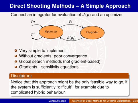
Direct Shooting Methods – A Simple Approach

Connect an integrator for evaluation of J(p) and an optimizer

p0 pi

p∗

φ(pi)

Very simple to implement

Without gradients: poor convergence

Global search methods (not gradient-based)

Gradients—sensitivity equations

Disclaimer

Notice that this approach might be the only feasible way to go, if

the system is sufficiently “difficult”, for example due to

complicated hybrid behaviour.


Multiple Shooting

Simultaneous method

Refinement of single shooting – divide horizon intoelements

Integrate each segment separately

Improvements over single shooting

Better numerical properties due to decoupling

State constraints at segment junctions

NLP larger than for single shooting but smaller than for

direct collocation

Popular in NMPC applications


Simultaneous Collocation Methods

Motivation

Integration of differential equations is expensiveSophisticated integrators are accurate, but not necessarilyconsistent

Very low tolerances[ long execution times

Noisy derivatives[ poor NLP convergence

Basic idea of simultaneous collocation methods:“Discretize not only the controls, but also the statevariables [ problem is transcribed into discrete form inone step

Not sufficient with a crude approximation: must fulfill

dynamic constraint with high accuracyThe resulting NLP is large (but sparse)


Collocation – Introduction

Given the dynamic system

x = f (x,u), x(t0) = x0

a simple method for solving the differential equation is

x (xk+1 − xkh

[ xk+1 = xk + h f (xk,uk)

where h = Ne/t f . Normally, we iterate, but what if we write all

equations simultaneously?

x1 − (x0 + h f (x0,u0)) = 0x2 − (x1 + h f (x1,u1)) = 0

...

xNe − (xNe−1 + h f (xNe−1,uNe−1)) = 0

[ c(x, u) = 0

System of Ne algebraic equations to be solved for the

unknowns x = (xT1 , . . . , xTNe)T , if u = (uT1 , . . . ,u

TNe)T assumed to

be known.Johan Åkesson Overview of Direct Methods for Dynamic Optimization—Collocation

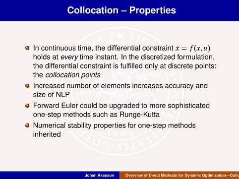
Collocation – Properties

In continuous time, the differential constraint x = f (x,u)holds at every time instant. In the discretized formulation,

the differential constraint is fulfilled only at discrete points:

the collocation points

Increased number of elements increases accuracy and

size of NLP

Forward Euler could be upgraded to more sophisticated

one-step methods such as Runge-Kutta

Numerical stability properties for one-step methods

inherited


Collocation and Optimization

Continuous time (infinite dimensional problem)

minu(t)

φ(x(t f )) s.t. x = f (x,u) x(0) = x0

Discrete time (finite dimensional problem)

minuk

φ(xNe), k = 0..Ne − 1

subject to

x0 + h f (x0,u0) − x1 = 0...

xNe−1 + h f (xNe−1,uNe−1) − xNe = 0

[ c(x, u) = 0

The infinite dimensional problem is transformed into a finite

dimensional static optimization problem


Additional Details

Path constraints straightforward, translates into algebraic

constraint

ci(x,u) ≤ 0[ ci(xi,ui) ≤ 0, i = 1..Ne

ce(x,u) = 0[ ce(xi,ui) = 0, i = 1..Ne

Terminal constraints are equally straightforward

ct(x(t f )) = 0[ ct(xNe,Nc) = 0

Minimum time problems can be formulated by optimizing

also over the element lengths hi and adding the constraint

Ne∑

i=1

hi = t f


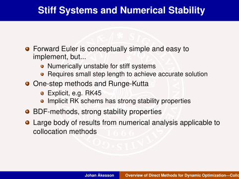
Stiff Systems and Numerical Stability

Forward Euler is conceptually simple and easy toimplement, but...

Numerically unstable for stiff systems

Requires small step length to achieve accurate solution

One-step methods and Runge-Kutta

Explicit, e.g. RK45Implicit RK schems has strong stability properties

BDF-methods, strong stability properties

Large body of results from numerical analysis applicable to

collocation methods


Optimization of Differential Algebraic Systems

Differential Algebraic Equations (DAEs)—generalized form

of ODEs

F(p, x, x,u,w, t) = 0, t ∈ [t0, t f ]

where p ∈ Rnp are the parameters, x ∈ Rnx are the state

derivatives, x ∈ Rnx are the states, u ∈ Rnu are the inputs

and w ∈ Rnw are the algebraic variables.

Assumptions (index-1 DAE)

F ∈ Rnx+nw∣

∣

[

�F�x ,

�F�w

]∣

∣ ,= 0

Intuition: given x we may solve for w and x (implicit

function theorem).

Index-1 DAEs are similar to ODEs, but solution of

non-linear equation systems may be needed to compute x

from x


Optimization of Differential Algebraic Systems

minp,uJ(p, q)

subject to

F(p,v) = 0, t ∈ [t0, t f ] DAEdynamics

F0(p,v) = 0, t = t0 Initial conditions

Ceq(p,v, q) = 0, Cineq(p,v, q) ≤ 0, t ∈ [t0, t f ] Path constraints

Heq(p, q) = 0, Hineq(p, q) ≤ 0 Point constraints

where

v =[xT , xT ,uT ,wT , t]T

q =[x(t1)T , x(t1)

T ,u(t1)T ,w(t1)

T , ...,

x(tntp)T , x(tntp)

T ,u(tntp)T ,w(tntp)

T ]T


Optimization Mesh

Divide the optimization interval into Ne intervals

Introduce normalized element lengths h0, . . . ,hNe−1 with

Ne−1∑

i=0

hi = 1

Element junction points

ti = t0 + (t f − t0)

i−1∑

k=0

hk, i = 1..Ne − 1

Radu collocation points τ j ∈ (0..1], j = 1..Nc in each

element gives

ti, j = t0+(t f − t0)

(

i−1∑

k=0

hk + τ jhi

)

, i = 0..Ne−1, j = 1..Nc


Piecewise Polynomial Variables

Approximate variable profiles using piecewise polynomials

t

z(t)

ti ti+1ti,1 ti,2 ti,3 ti+1,1 ti+1,2 ti+1,3

zi,1zi,2 zi,3

zi+1,1zi+1,2

zi+1,3

Element i Element i+ 1

z(t) =

Nc∑

j=1

zi, jL j

(

t− ti−1hi

)

t ∈ [ti−1, ti], hi = ti+1 − ti

L j are interpolation polynomials


Lagrange Polynomials

Given Nc points, τ1, . . . ,τNc ∈ [0, 1], the corresponding

Lagrange polynomials are given by

L(Nc)j (τ ) = 1 if Nc = 1

L(Nc)j (τ ) =

Nc∏

k=1,k,= j

τ − τ kτ j − τ k

if Nc ≥ 2

Property of Lagrange polynomials

L(Nc)j (τ k) = δ j,k, i.e.,

L(Nc)j (τ k) =

{

1, if j = k0, if j ,= k

It follows that

z(ti, j) =

Nc∑

k=1

zi,kL(Nc)k

(

ti, j − ti−1hi

)

=

Nc∑

k=1

zi,kL(Nc)j (τ k) = zi, j


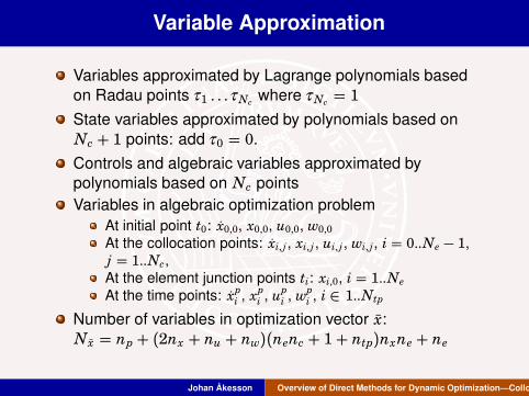
Variable Approximation

Variables approximated by Lagrange polynomials based

on Radau points τ1 . . .τNc where τNc = 1

State variables approximated by polynomials based on

Nc + 1 points: add τ0 = 0.

Controls and algebraic variables approximated by

polynomials based on Nc points

Variables in algebraic optimization problem

At initial point t0: x0,0, x0,0, u0,0, w0,0At the collocation points: xi, j , xi, j , ui, j , wi, j, i = 0..Ne − 1,j = 1..Nc,At the element junction points ti: xi,0, i = 1..NeAt the time points: x

pi , x

pi , u

pi , w

pi , i ∈ 1..Ntp

Number of variables in optimization vector x:

Nx = np+ (2nx + nu + nw)(nenc + 1+ ntp)nxne + ne


Equality Constraints

Initial equations

F0(p,v0,0) = 0, v0,0 = [xT0,0, x

T0,0,u

T0,0,w

T0,0, t0]

T

DAE dynamics at collocation points

F(p,vi, j) = 0, i = 0..Ne − 1, j = 1..Nc

Continuity of state profiles

xi,nc − xi+1,0 = 0, i = 0..Ne − 1

Control variables at initial point (interpolation

u0,0 =

(Nc)∑

k=1

u0,kLNck(0)

Collocation equations

xi, j =1

hi(t f − t0)

Nc∑

k=0

xi,kL(Nc+1)k

(τ j), i = 0..Ne−1, j = 1..Nc


Equality Constraints cont’d

Interpolation of variables at time points

xp

l =1

hil (t f−t0)

Nc∑

k=0

xil ,k L(Nc+1)k (τ pl ), l = 1..ntp

xp

l=

Nc∑

k=0

xil ,kL(Nc+1)k

(τ pl), l = 1..ntp

upl =

Nc∑

k=1

uil ,kL(Nc)k (τ pl ), l = 1..ntp

wpl =

Nc∑

k=1

wil ,kL(Nc)k (τ pl ), l = 1..ntp

Total number of equality constraints resulting from

discretization of dynamics: 2nx + nw + (nx + nw)NeNc +nxNe + nu + nxNeNc + (2nx + nu + nw)ntp

Degrees of freedom of algebraic optimization problem:

np + nuNeNc


A Non-Linear Program

Non-Linear program resulting from collocation

minxf (x)

subject to

�(x) ≤ 0

h(x) = 0

� contains point and path inequality constraints Cineq and

Hineq

h contains point and path equality constraints Cineq and

Hineq in addition to dynamic constraints


Collocation with Lagrange Polynomials – Properties

Equivalent to an implicit Runge-Kutta one-step method

Large body of applicable theory from numerical analysis

Good numerical stability properties

Applicable to stiff (( numerically difficult) systems

State and control constraints straightforward

Handles unstable systems

Accurate derivatives essential for convergence

The NLP problem is usually very large but sparse, must be

exploited for efficiency


What can go wrong?

Convergence of gradient based methods relies on a twice

continuous differentiable right-hand side (( smooth

f (x,u))

[ Discontinuities may cause problemif-clauses (which introduce discontinuous)

Avoid, if possible (or use a method explicitly adressing

discontinuities)

abs, min and max functions

Use max(x, y) = ((x − y)2 + ǫ2)0.5/2+ (x + y)/2

Saturation

Use smooth approximation (can be constructed from smooth

min and max approximations)

Lookup-tables

Use sufficiently smooth spline interpolations instead of linear

interpolation

Scaling problems (especially for simultaneous methods)

Need a reasonable initial guess (use simulation)


Documents

Overview of Direct Methods for Dynamic Optimization ... · Johan Åkesson Overview of Direct Methods for Dynamic Optimization—Collocation. Optimization of Differential Algebraic