Embed Size (px)
Citation preview

7/21/12
1
IntroductorySta1s1csandGraphics
DeborahNolanUniversityofCalifornia,Berkeley
Overview• Background&Mo1va1on• Studentswillbeableto…• Exampleassignments
• Studentworkandfeedback• Samplelecturematerialongraphics
Background&Mo1va1on
Tradi1onalSyllabus:• Timespentongraphicsisshort• Typesofplotsshownaresimple(histogramandscaOerplot)
• BalanceoftopicsisinfavorofConfirmatoryDataAnalysisratherthanExploratoryDataAnalysis
• Visualcommunica1onofresultsislacking

7/21/12
2
Syllabushasmoreemphasison• Datatypes,subsets,&comparisons–soknowwhattype
ofplotandanalysisisappropriate• Summarysta1s1csfolloweasilyfromsummaryplots• Introduc1ontoR–neededtomakeplots• Mul1variatesta1s1cs–onceworkingonthecomputer,
it’snaturaltocovermorethanunivariateandbivariatesitua1ons
• Presenta1onGraphics–howtocommunicateyourfindingseffec1velythroughafewkeyplots
Poten1alwithGraphics:• Alterna1veapproachtolearningconcepts
– Construc1ve– Methodofcomparison,varia1on,distribu1on
• Studentusevisualiza1onthroughoutthecourse(notjustatthebeginning)– Crea1veandmeaningfuldataanalysis– Discoverythroughvisualiza1on
• Opportunitytointroducemoremodernmethods– Excitestudentstostudysta1s1cs
Studentswillbeableto:
Analysis:• CarryoutExploratoryDataAnalysistouncoverstructureindata
• Usedatavisualiza1onsasafirststepinmodeling
• Integratetheuseofgraphicsthroughouttheanalysisprocess,includingconfirmatoryandrepor1ngstages

7/21/12
3
Communica1on:• Describeagraphicusingacommonvocabulary• Readandthinkcri1callyaboutagraphic• Createagraphicthatconveyskeypointsofananalysis
• Createpresenta1ongraphics,i.e.– Appropriateuseofscale,color,labels,markers
Technicalskills:• Chooseappropriategraphicfordifferenttypesofdata
• Designaplotthatconveysamessageclearlyandprecisely
• Entrypointforlearningsta1s1calso]ware
GraphicsAssignments
Assignments1) Afirstexploratoryassignment2) Deconstruct‐reconstruct3) One‐minuterevela1on
4) Mashup/Newformofpresen1ngdata(advanced)
5) CopytheMasters(advanced)

7/21/12
4
AFirstExploratoryAssignment• Providestudentswithdataandanopen‐endedques1ontoinves1gate
• AssignmentIncludesintermediateques1onsthatpromotethemethodofcomparison
• StudentsUseONLYplotstodiscoverfeaturesofthedata
• Studentswriteashortpaperonfindings
AFirstExploratoryAssignment
• Assignitearlyinthesemestertosetexpecta1onsofcon1nuedanalysiswithplots
• Use“large”data(~1000observa1ons,manyvariables)sotheop1onofvisualinspec1onofrawdataisnotgoingtowork
• Requiretheuseofone“unusual”plottoencouragecrea1vity
Deconstruct–reconstruct• EachpairofstudentsChoosesaplotthatsa1sfiesthefollowing:– Topicofinteresttothestudents– Understandthemessagetheplot‐makeristryingtoconvey
– CanimproveonthemessagewithabeOerplot– Source–fromacollabora1vevisualiza1onsite
Deconstruct–reconstruct• Deconstruct–Writeacap1onfortheplotthat:– Explainsthemessageintheplot
– Describestheplotusingplojngvocabulary– Cri1quesplotaccordingtoguidelinesofgoodgraphics

7/21/12
5
Deconstruct–reconstruct• Reconstruct
– Remakeplot,fixingtheissuesfound– Augmenttheplotwithaddi1onalinforma1onthatmakesthemessageclearer
– Writeacap1onthatexplainsthemessagebypoin1ngoutimportantfeaturesintheplot
ExampleStudentWork
One‐minuterevela1on• Studentsworkinteamsonadataset• Eachstudentontheteamcreatesoneplotthatrevealsanimportantfeatureofdata
• EachstudentPrepares1‐minutedescrip1onoftheplot
• Coordinateplot&presenta1onwithteammembers
One‐minuterevela1on• Purpose
– Getstartedonteamproject– Makeeachstudenttakepartintheanalysis
– Getteamworkingtogether– Studentsreceiveearlyinputfrominstructor– Skillsusefulinworkplace

7/21/12
6
IndoorRadonLevels(StatLabs)• Radon‐radioac1vegas
emiOedfromsoil,rock,water;canaccumulatetounsafelevels
• Data:SurveyresultsofradonlevelsforhousesinMinnesota
• Ques1on:Howdowees1materadonlevelsforuntestedhousesanddecideifhouseshouldbetested?
Mashup/Newformofpresenta1on• Viewersexpecttointeractwithgraphicalrepresenta1onsofdata:– Obtainaddi1onalinforma1on– Produceadifferentview– Controlananima1on
• GoogleMaps,GoogleEarth–RKML• Modelsforcrea1nginterac1vity
Earthquakeloca1ons
7/21/12
7
ElephantSealMovementsRScaOerplotGoogleEarth–anima1on
Copythemasters• Assignment
– Createanear‐replicaofamasterfulpresenta1on
• Purpose– Learnso]ware– Learnhowtolearnaboutatechnicalsubject– BecomeinvestedinRasasta1s1caltool– Gainprac1cewithadvanced/presenta1ongraphics

7/21/12
8
StudentFeedback
Deconstruct‐reconstruct(75of111)
CopyMasters:(18of25)• HelpedtolearnRbasics‐Yes:18/18• Expecta1onstoresearchcommandsonownwasagoodlearningprocess‐Yes:16/18
• Samplecomments– Mostmemorableassignment– Mostchallengingandrewardingassignment– Ifeltmuchmoreconfidentaboutmyabili1eswR
TwoSampleLectures
7/21/12
9
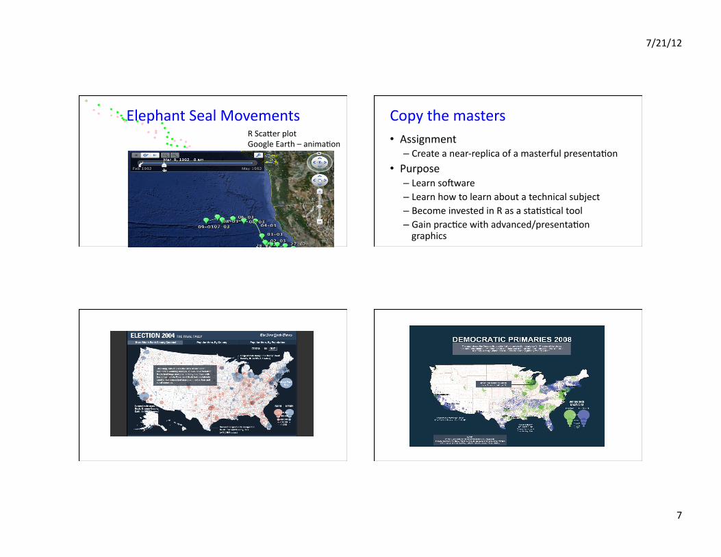
IntroductoryMaterial
IntroductoryLessonApproach
• Embedintroduc1ontoplotsandothersta1s1csincontextofacasestudy
• Begincoursewithgraphicsandmodelforthestudentshowtoreadaplotandextractmeaningfromit
IntroductoryLessonApproach• Demonstratehowplojngisanitera1veprocess
• Connectgraphicstoallsta1s1calconceptsthroughoutthecourse
• Con1nuetoconnectthechoiceofaplottothetypeofdatathroughoutthecourse
KnowyourdatatypesTheappropriategraphicaltechniquesdependonthekindofdatathatyouareworkingwith• Quan1ta1ve
– con1nuous–e.g.height,weight– discrete–numericdatawithfewvalues,e.g.numberofchildreninfamily
• Qualita1ve– ordered–categorieswithanorderbutnomeaningfuldistancebetween,e.g.numberofstarsforamoviera1ng
– nominal‐categorieshavenomeaningfulorder,e.g.race

7/21/12
10
KaiserStudy• OaklandKaisermothers• 1960s• Measurethebabiesweight(inounces)atbirth• Allbabies:
– Male– Singlebirths(notwins,etc.)– Survived28days
Informa1ononmothers&babies• Birthweight(ounces)• Gesta1on(weeks)• Parity‐totalnumberofpreviouspregnancies• Mother’sheightandweight• Mother’ssmokingstatus• Mother’sage,race,educa1onlevel,income• Andmore…
HerearethedataforbirthweightWhatdoyousee?
[1]1201131281231081361381321201431401441411101141159211514411910511513712213110314611412511412293130119113134[37]107134122128129110138111871431551101221451151081021431461241241451067510712412210112810497137103142130156[73]1331209112715312112099149129139114138129138131125114]128134114928513587125128105120119116107119133155126[109]12913710312591134951181411311211001311181521211171151129410913211710111212812811713412793122100147120144[145]105136102160113126126115127119129123118133105134144111125135134116129113131126121121138136120122134101112132[181]13611396124113131137133107961421367512510413090118123137101142981241511091501191311011131279711715085[217]1281059011510712111911713411711511013014011193154125931221291268517314411411115415011112612214114299113[253]14911713010612812511413011681124125110125138142115102140133127104119152123143131141129113119109104131110148[289]13711711598136121132911198510613280109111143136110981081017112493106101100104117117149135110121142104[325]13811211710913112011614010312013912310413111112211612913311010593122133130104106120121118140114116129120127[361]107718810712210613510712912611612412314510212998110135101961041001541271261261279812712913113212799115[397]14510213612112112011812713210214311810216313211613813913287131130123115116119125144123120140120116120146112[433]1151321461221281191351161291161001181381231131291221321201141301171421441271158599123112681021091029978[469]128107136101100109117889511912312710712412698961041339310111813012514011513011410510113211269114123129[505]1141159812811911915412713112911411010311713812612411113210315814610113211471116108123129134113123147121125[541]115101931091151301231119712212412912410714212917410510312410513316110510815313311512712811712311914191116[577]1161211111021181269813111510314712312511799115116118170104108144999714285130117109147105135115123105154[613]11011910311712014510412312412991109108791331141281299710317614312710711310615215013615112412311912211293[649]109136121150941201461291251241419613812711410312714111399971161261581191231291171001311468411511511891[685]112115110117109991311361301341281508611514178100116110109113136114121117166871209513290131103144137124[721]1361171211161391108613381133132132137841369211412916771124105155125125125115174127113115139127111112143[757]116155121110871321051291239114714412813710412011213896134126112138110831121481198611012612513612784131[793]12396110123152127117125139114961241071139811910711711714413612116512012513710013488108123141130139130113[829]7762931091459212013511312614312898110162116128111137134100160112134145116126111126109136119103124155122[865]113122126116102110133125164133135124122121100129901281168612387128120125118116131151881371279612912885[901]11112411211572122116127909914413858109110129150128142115108108139115136163131771241041029415811211997[937]991151391449910589129119114106122136121112112123139125105130146133147109122135107117138120119118105113136[973]148140134120123102551031231051381281391041591189914412111711910512511910110511010098127117122122118137120[1009]143108131110105133125781141111031147516994150144144143145121105134129114971606514595139123109110122115[1045]117108120131136125961021021121359112915510980125941487312365118102120108122103105126145139124121126119[1081]1141181271171371331001071159111212515710813013512310012417412911912612811610096131110108129141110118111160[1117]120121113117158128158133163128126127134140102100120981301041221371146398998911714310699156727597106[1153]91117117112112141131130132114160106841121391041307182119123115124138881461288210011497126122152116132[1189]841191041061241391031129610212010297113130971161141278714114411675138991181529714681110135114124115[1225]143113109103118127132113128130125117
Rugplot
Birth Weight
60 80 100 120 140 160 180
Baby’sbirthweightisrepresentedasa1ckmark.Thethickerlinesarefrommul1plebabieswithsimilarweights.IaddedaliOlerandomnoisetotheweightstokeepthemfromfallingontopofeachother.Whatcanyouseenow?Howarebirthweightsdistributed?

7/21/12
11
Distribu1onofBirthWeight• Thedistribu6onisthepaOernofvaria1oninthebirthweights.
• Itprovidesthenumericalvaluesforbirthweightandhowo]eneachvalueoccurs.
• Ahistogram/densityplotshowstheshapeofthedistribu1on
Histogram: hist(infants$bwt)
hist(infants$bwt,freq=FALSE,xlab="BirthWeight(oz)",main="MaleBabies,OaklandKaiser1960s")
Histograms• Areaspecialcaseofdensityplots• AREA=Propor1on(orpercent)• Theareaofabar:
Height*Width=Area(Propor1on/oz)*oz=Propor1on
• Histogramsarenotthesameasbarcharts• Withbarcharts,itisonlytheheightthatmaOers.Barchartsareforqualita6vedata
Densityplot–smoothedhistogramplot(density(infants$bwt))
50 100 1500.000
0.005
0.010
0.015
0.020
Male babies born at Oakland Kaiser in the 1960s
Birth Weight (oz)
Den
sity
(pro
porti
on p
er o
z)
plot(density(infants$bwt), xlab = "Birth Weight (oz)", main = "Male Babies, Oakland Kaiser 1960s")

7/21/12
12
Babiesbirthweightplot(density(infants$bwt, bw = 1))
60 80 100 120 140 160 180
0.000
0.005
0.010
0.015
0.020
0.025
Male babies born at Oakland Kaiser in the 1960s
Birth Weight (oz)
Den
sity
(pro
porti
on p
er o
z)Selec1ngabandwidth
• Rchoosesabandwithforyou,butyoucanspecifyoneifyoulike.
• Thegoalistoseetheoverallshapeofthedistribu1on,nottheindividualpoints.
• Inaway,thedensityisasmoothabstrac1onofthedistribu1on.
Boxplot:boxplot(infants$bwt)
boxplot(infants$bwt, xlab="Birth Weight (oz)")
LookingforStructure:Quan1ta1veDistribu1on
• Distribu6on:paOernofvaluesforavariable• Mode:highdensityregion• LongTail:manyobserva1onsfarfromcenter• Symmetry/Skewness:distribu1onofvaluesthele]andrightofthecenter.
• Gaps:placeswheretherearenoobserva1ons.• Outliers:unusuallylargeorsmallvaluesthatfallswellbeyondtheoverallpaOernofdata

7/21/12
13
WhatStructureDoYouSee?
Parity:Numberofsiblings• Thisquan1ta1vevariableisdifferentfrombirthweight–thereareonlyafewpossiblevalues,i.e.it’snotpossibletohave2.3siblings,andit’shighlyunlikelytohave17
>table(infants$parity) 01234567891011133153102381688352321687421
NumberofSiblings
0 1 2 3 4 5 6 7 8 9 11Number of siblings
050
150250
barplot(table(infants$parity))
Alterna1ve–barwidthhasnomeaning
0.00
0.10
0.20
Number of siblings
Prop
ortion
0 1 2 3 4 5 6 7 8 9 11 13plot(table(infants$parity), type="h", lwd = 4, ylab="Proportion", col="darkgrey")

7/21/12
14
Survey• RandomSampleof91of314CalstudentsenrolledinStat2
• Surveycollectedthefollowinginfo:– sex–Male/Female– grade–gradeexpectedinthecourse(“A”,“B”,“C”,“D”,“F”)
• Whattypeofdataarethese?– sexisqualita1ve(nominal)– gradeisqualita1vewithanordering(ordinal)
Maketablesofqualita1vedata> table(video$grade) FDCBA0085231>table(video$grade,video$sex)FemaleMaleF00D00C80B2131A922
Anythingunusualabouttheexpectedgrade?
Doesexpectedgradedependongender?
ExpectedGradeBarchart
Piechartpie(table(video$grade))
F D C B A
010
20
30
40
50
C
B
A
AREAScanbehardtocompare
WIDTHofbarshavenomeaning
ExpectedGradeDotchartdotchart(table(video$grade), pch = 19)
FDCBA
●
●
●
●
●
0 10 20 30 40 50
Focusoncomparisonofthevalues

7/21/12
15
MethodofComparison• O]en,wenotonlywanttobeOerunderstandadistribu1on,butwewanttocomparethedistribu1onforsubgroupsortocompareagainstanotherpopula1onorstandard
• Howdoyouthinktheexpectedgradedistribu1onmightvarywithgender?
TwoQualita1vevariablesStat 2 Survey
sex
grade
Female Male
FD
CB
A
mosaicplot(table(video$sex,video$grade),main="Stat2Survey")
HowtoreadaMosaicplot
Thereare91studentsinthesurvey.Thinkofthemasspreadoutevenlyinthebox
NewPlot:Mosaic
Putallthefemalesononesideofthebox.Thereare38.

7/21/12
16
NewPlot:Mosaic
Rearrangethefemalessothatthosewhoexpectthesamegradearetogetherinthebox.8ofthe38expectaC
MosaicplotStat 2 Survey
sex
grade
Female Male
FD
CB
A
Smallerfrac1onoffemalesexpectanAincomparisontoMales
NoneofthemalesexpectaC
SFHousingDataVariables:• City• County• Price• #bedrooms• Lotsquarefootage• and10more
• Record:housesoldinapar1cular1meperiod
• Over200,000houses• Subsettoadozenci1esin
theEastBay–about25,000houses
Rela1onshipbetweencityandsaleprice
Datatypes:City‐factorSaleprice‐numeric

7/21/12
17
boxplot(shousing$price ~ shousing$city, las = 2)
Boxplots Ci1esorderedbymedianprice
Rela1onshipbetweenpricepersquarefootandtotalsquarefoot
Botharequan1ta1ve
ppsf = shousing$price/shousing$bsqft plot(ppsf ~ shousing$bsqft)
WHAT’sWrongwiththisplot?

7/21/12
18
Rela1onshipsbetweenmorethan2variables
• Qualita1veinforma1oncanbeconveyedinplotsthroughcolor,plojngsymbol,juxtaposedpanels
• Thefollowingplotusesinforma1onfrom4variables:city,numberofbedrooms,lotsize(sq]),andpricepersquare]
!
!
!
!
!
!
!
!
!
!
!
!
!
!
!
!
!
!
!
!
!
!
!
!
!
! !
!
!
!
!
!
!
!
!
!
!
!
!
!
!
!
!
!
!
!
!
!
!
!
!
!
!
!
!
!
!
!
!
!
!
!
!
!
!
!
!
!
!
!
!!
!
!
!
!
!
!
!
!
!
!
!
!
!
!
!
!
!
!
!
!
!
!
!
!
!
!
!
!
!
!
!
!
!
!
!
!
!
!
!
!
!
!
!
!
!
!
!
!
!
!
!
!
!
!
!
!
!
!
!
!
!
!
!
!
!
!
!
!
!
!
!
!
!
!
!
!
!
!
!
!
!
!
!
!
!
!
!
!
!
!
!
!
!
!
!
!
!
!
!
!
!
!
!
!
!
!
!
!
!
!
!!
!
!
!
!
!
!!
!
!
!
!
!
!
!
!!
!
!
!
!
!
!
!
!
!
!!
!
!
!
!!
!
!
!
!!
!!
!!
!
!
!
!
!!
!
!
!
!
!
!
!
!
!
!
!
!
!
!
!
!
!
!
!
!
!
!
!!
!!
!
!
!
!
!
!
!
!
!
!
!
!
!!
!
!
!
!
!
!!
!
!
!
!
!
!
!
!
!
!
!
!!
!
!
!
!
!
!
!
!
!
!
!
!!
!!
!
!
!
!
!
!
!
!
!
!
!
!
!
!
!
!
!
!
!
!
!
!
!
!
!
!
!
!
!
!
!
!!!
!
!
!
!
!
!
!
!
!
!
!
!
!
!
! !
!
!
!
!
!
!
!
!
!
!
!
!
!
!
!
!
!
!
!
!
!
!
!
! !
!
!
!
!
!
!
!
!
!
!
!
!
!
!
!
!
!
!
!
!
!
!
!
!
!
!
!
!
!
!
!
!
!
!
!
!
!
!
!
!
!
!
!
!
!
!
!
!!
!
!
!
!
!
!
!!
!
!
!
!
!
!
!
!
!
!
!
!!
!
!
!
!
!
!
!
!!
!
!
!
!
!
!
!!
!
!
!
!
!
!
!
!
!
!
!
!
!
!
!
!
!
!
!
!
!
!!
!!
!
!
!
!
!
!
!
!
!
!
! !!
!
!
!
!
!
!
!
!
!
!
!
!
!
!
!
!
!
!
!
!
!
!
!
!
!
!
!
!
!
!!
!
!
!
!
!
!
!
!
!
!
!
!
!
!
!
!
!
!
!
!
!
!
!
!
!
!
!
!
!
!
!
!
!
!
! !
!
!
!
!
!!!
!
! !
!
!
!
!!
!
!
!
!
!
!!!
!
!
!
!
!
!
!
!
!
!
!
!
!
!!
!
!
!
!!
!
!
!
!
!
!
!
!
!
!
!
!
!
!
!
!
!
!
!
!
!
!
!
!!
!
!
!
!
!
!
!
!
!
!
!
!
!
!
!
!
!!
!
!
!
!
!
!
!
!
!
!
!
!
!
!
!
!
!
!
!
!!
!
!
!
!
!
!
!
! !!
!
!
!
!
!
!
!
!
!
!
!
!
!
!
!
!
!
!
!
!
!
!
!
!
!
!
!
!
!
!
!
!
!
!
!
!
!
!
!
!
!
!
!
!!
!
!
!
!
!
!
!
!
!
!
!
!
! !
!
!
!
!
!
!
!
!
! !
!
!
!
!
!
!
!
!
!
!
!
!
!
!
!
! !
!
!
!
!
!
!
!
!
!
!
!
!
!
!
!
!
!
!
!
!
!
!
!
!
!!
!
!
!
!
!
!
!
!
!
!
!
!
!
!
!
!
!
!
!
!
!
!
!
!
!
!
!
!
!
!
!!
!
!
!
!!
!
!!
!
!
!
!
!
!
!
!
!
!
!
!
!
!
!
!!
!
!
!
!
!
!
!
!
!
!
!
!
!
!
!
!
!
!
!!
!
!
!
!
!
!
!
!
!
!
!
!
!
!
!
!
!
!
!!
!
!
!
!
!
!
!
!!
!
!
!
!
!
!
!
!
!
!
!
!
!
!
!
!
!
! !
!
!
!
!
!
!
!
!
!
!
!
!
!
!
!
!
!
!
!
!
!
!
!
!
!
!
!
!
!
!
!
!
!
!
!
!!
!
!
!
!
!
!
!
!
!
!
!
!
!
!
!
!
!
!
!
!
!
!
!
!
!
!
!!
!
!
!
!
!
!
!
!
! !
!
!
!
!
!
!
!
!
!
!
!
!
!
!
!
!
!
!
!
!
!
!
!
!
!
!
!
!
!
!
!
!
!
!
!
!
!
!
!
!
!
!
!
!
!
!
!
!
!
!
!
!
!
!
!
!
!
!
!
!
!
!
!
!
!
!
!
!
!
!
!
!
!
!
!
!!
!
!
!
!
!
!
!
!
!
!
!
!
!!
!
!
!
! !
!
!
!
!
!
!
!
!
!
!
!
! !
!
!
!
!
!
!
!
!
!
!
!
!
!
!
!
!
!
!
!
!
!
!
!
!
!
!
!
!!
!
!!
!
!
!
!
!
!
!
!
!
!
!
!
!
!
!
!
!
!
!!
!
!
!
!!
!
!
!
!
!
!
!
!
!
!
!
!
! !
!
!
!
!
!
!
!
!
!
!
!
!
!
!
!
!
!
!!
!
!
!
!
!
!
!
!
!!
!
!
!
!
!
!
!
!
!
!
!
!
!
!
!
!
!
!
!
!
!
!
!
!
!
!
!!
!
!
!
!
!
!
!!
!!
!
!
!
!
!
!
!
!
!
!
!
!
!
!
!
!
!
!
!
!
!
!
!
!
!
!
!
!
!
!
!
!
!
!
!
!
!
!
!
!
!
!
!
!
!
!
!
!
!
!
!
!
!
!
!
!
!
!
!
!
!
!
!
!
!
!
!
!
!
!
!
!
!
!
!
!
!
!
!
!
!
!
!
!
!
!
!
!
!
!!
!
!
!
!
!!
!
!
!
!
!
!
!
!
!
!
!
!
!!
!
!
!
!
!
!
!!
!
!
!
!
!
!
!
!
!
!
!
!
!
!
!!
!!
!
!
!
!
!
!
!
!
!
!
!
!
!
!
!
!
!
!
!
!
!
!
!
!
!
!!
!
!
!
!
!
!
!
!
!
!
!
!
!
!
!
!
!
!
!
!
!
!
!
!
!
!
!
!
!
!!
!
!
! !
!
!
!
!
!
!
!
!
!
!
!
!
!
!
!
!
!
!
!
!
!
!
!
!
!
!
!
!
!
!
!
!
!
!
!
!
!
!
!
!
!
!
!
!
!
!
!
!
!
!
!
!
!
!
!
!
!
!
!
!
!
!
!
!
!
!
!
!
!
!
!
!
!
!
!
!
!
!
!
!
!
!
!
!
!
!
!
!
!
!
!
!
!
!
!
!
!
!
!
!
!
!
!
!
!
!
!
!
!
!
!
!
!
!
!
!
!
!
!
!
!
!
!
!
!
!
!
!
!
!
!
!
!
!
!
!
!
!
!
!
!
!
!
!
!
!
!
!
!
!
!
!
!
!
!
!
!
!
!
!
!
!
!
!
!
!
!
!
!
!
!
!
!
!
!
!
!
!
!
!
!
!
!
!
!
!
!
!
!
!
!
!
!
!
! !
!
!!
!
!
!
!
!
!
!
!
!
!!
!
!
!
!
!
!
!
!
!
!
!
!
!
!
!
!
!
!
!
!!
!
!
!
!
!
!
!
!
!
!
!
!
!
!!
!
!
!
!
!
!
!
!
!
!
! !
!
!
!
!
!
!
!
!
!
!
!
!
!
!
!
!
!
!
!
!
!
!
!
!
!!
!
!
!
!
!
!
!
!
!
!
!
!
!
!
!
!
!!
!
!
!
!
!
!
!
!
!
!
!
!
!
!!
!
!
!
!
!
!
!
!
!
!
!
!
!
!
!
!
!
!
!
!
!
!
!
!
! !
!
!
!
!
!
!
!
!
!
!
!
!
!
!
!!
!
!
!
!
!
!
!
!
!
!
!
!
!
!
!
!
!
!
!
!
!
!
!!
!
!
!!
!
!
!
!
!!
!
!
!
!
!
!!
!
!
!
!
!
!
!
!
!
!
!
!
!
!
!
!
!
!
!
!
!
!
!
!
!
!
!
!
!
!
!!
!
!!
!
!
!
!
!
!
!
!
!
!
!
!
!
!
!
!
!
!
!
!
!
!
!
!
!
!
!
!
!
!
!
!
!
!
!
!
!
!
!
!
!
!
!
!
!
!
!
!
!
!
!
!
!
!
!
!
!
!
!
!
!
!
!
!
!
!
!
!
!
!
!
!
!
!
!
!
!
!
!
!
!
!!
!
!
!
!
!!
!
!
!
!
!
!
!
!
!
!
!
!!
!
!
!
!
!
!
!
!
!
!
!
!
!
!
!!
! !
! !!
!
!
!
!
!
!
!
!
!
!
!
!
!
!
!
!
!
!
!
!
!
!!
!
!
!
!
!
!
!
!
!
!
!
!
!
!
!
!
!
!
!
!
!
!
!
!
!
!
!
!
!
!
!
!
!
!
!
!
!!
!
!!
!
!!
!!
!
!
!
!
!
!
!
!
!
!
!
!
!
!
!
!
!
!
!
!
!
!
!
!
!
!
!
!
!
!
!
!
!
!
!
!
!
!
!
!
!
!
!
!
!
!
!
!
!
!
!
!
!
!
!
!
!
!
!
!
!
!
!
!
!
!
!
!
!
!
!
!
!
!
!!
!
!
!
!
!
!
!
!
!
!
!
!
!
!!
!
!
!
!
!
!
!
!
!
!
!
!
!
!
!
!
!
!
!
!
!
!
!
!
!
!
!
!
!
!
!
!
!
!
!
!!
!
!
!
!
!
!
!
!
!
!
!
!
!
!
!
!
!
!
!
!!
!
!
!
!
!
!
!
!
!
!
!
!
!
!
!
!
!
!
!
!
!
!
!
!
!
!
!
!
!
!
!!
!
!
!
!
!
!
!
!
!
!
!
!!
!
!
!
!
!
!
!!
!
!
!!
!
!
!
!
!
!
!
!
!
!
!
!
!
!
!
!
!
!
!
!
!
!
!
!
!
!
!
!
!
!
!
!
!
!
!
!
!
!
!
!
!
!
!
!
!
!
!
!
!
!
!
!
!
!
!
!
!
!
!
!
!
!
!
!
!
!
!
!
!
!
!
!
!
!
!
!
!
!
!
!
!
!
!
!
!
!
!
!
!
!
!
!
!
!
!!
!
!
!
!
!
!
!
!
!
!
!
!
!
!
!
!
!
!
!
!
!
!
!
!
!
!
!
!
!
!
!
!
!
!
!
!
!
!
!
!
!
!
!
!
!
!
!
!
!
!
!
!
!
!
!
!
!
!
!
!
!
!
!
!
!
!
!
!
!
!
!
!
!!
!
!
!
!!
!
!
!
!
!
!
!
!
!
!
!
!
!
!
!!
!
!
!
!
!
!
!
!
!
!
!
!
!
!
!
!
!
!
!
!
! !
!
!
!
!
!
!
!
!
!
!
! !
!
!
!
!
!
!
!
!
!
!
!
!
!
!
!
1000 2000 3000 4000 5000
200
400
600
800
Berkeley
Square Feet
Pri
ce p
er s
quar
e fe
et
1 bedrooms
2 bedrooms
3 bedrooms
4 bedrooms
5 bedrooms
6 bedrooms
7 bedrooms
8 bedrooms!
!
!
!
!!!
!
!
!
!
!
!
!
!
!
!
!
!
!
!
!!
!
! !
!
!
!
!
!
!
!
!
!
!
!
!
!
!
!!
!
!
!
!
!
!
!
!
!
!
!
!
!
!
!
!
!
!
!
!
!
!
!
!
!
! !
!
!
!
!
!!
!
!
!
!
!
!
!
!
!
!
!
!
!
!
!
!
!
!
!
!
!
!
!
!
!
!
!
!
!
!
!
!
!
!
!
!!!
!
!
!
!
!
!
!
!
!
!
!
!
!
!
!
!
!
!
!
!
!
!
!
!
!
!!
!
!
!
!
!
!
!
!
!
!
!
!
!
!
!
!!
!
!
!
!
!
!
!
!
!!
!
!
!
!
!
!!
!
!
!!
!
!
!
!!
!
!
!
!
!
!
!
!
!
!
!
!
!
!
!
!
!
!
!!
!
!
!
!
!
!!
!
!
!
!
!
!
!
!
!!
!
!
!
!
!
!
!
!
!
!
!!
!
!
!!
!
!
!
!
!
!
!
!
!
!
!
!
!
!
!
!
!
!!
!
!
!
!
!
!
!!
!!
!
!
!
!
!
!
!!
!
!
!
!
!
!
!
!
!
!
!
!!
!!
!
!
!
!
!
!
!
!
!
!
!
!
!
!
!
!
!
!
!
!
!
!
!
!
!
!
!
!
!
!
!
!
!
!
!
!
!!
!
!
!
!
!
!
!
!
!
!
!
!
!
!
!
!
!
!
!
!
!
!
!!
!
!
!!
!
!
!
!
!
!
!
!
!
!
!
!
!!
!
!
!
!
!
!
!
!
!
!
!
!
!
!
!
!
!
!
!
!
!
!
!
!
!
!
0 1000 2000 3000 4000 5000
200
400
600
800
Piedmont
Square Feet
Pri
ce p
er
square
feet
1 bedrooms
2 bedrooms
3 bedrooms
4 bedrooms
5 bedrooms
6 bedrooms
7 bedrooms
8 bedrooms
Whatdoyousee?Summaryofgraphrela1onships
betweentwovariables
• TwoQualita1vevariables– mosaicplot,side‐by‐sidebarplots
• OneQuan1ta1veandoneQualita1ve– Boxplots,dotcharts,mul1pledensityplots,violinplots
• TwoQuan1ta1vevariables– ScaOerplot,lineplot

7/21/12
19
ElementsofGoodGraphicConstruc1on
Outline• Vocabulary• 3Proper1esofgoodgraphconstruc1on
– Datastandout– Facilitatecomparison
– Informa1onrich
• Percep1on
Vocabulary ! !
!
!
!
!
! !
!
!
!
!
!
!
!
!
!
!
!
! !
!
!
!
!
! !
!
! !
Axis Label: Day
! !
!
!
!
!
! !
!
!
!
!
!
!
!
!
!
!
!
! !
!
!
!
!
! !
!
! !
10 15 20 25 30tick
marktick
mark
label
Reference line: 75
Verti
cal A
xis
plotting
symbol
Title: Temperature in August
data label
Min: Aug 17 over 70
below 70
Legend

7/21/12
20
DataStandOut
Avoidhavingothergraphelementsinterferewithdata
! !
!
!
!
!
! !
!
!
!
!
!
!
!
!
!
!
!
! !
!
!
!
!
! !
!
! !
Day
1 3 5 7 9 12 15 18 21 24 27 30
Usevisuallyprominentsymbols
! !
!
!
!
!
! !
!
!
!
!
!
!
!
!
!
!
!
! !
!
!
!
!
! !
!
! !
0 5 10 15 20 25 30
6570
7580
Day
Degrees
Avoidover‐plojng
!
!
!
!
!
!
!
!
!
! !
!
!
!
!
!!
!
!
!!! !
!
!
!
!
!
!
!
!
!
!
!
!
!
!
!
!
!
!
!
!
!
!
!!
!
!
!
!
!
!
!
!
!
!
!
!
! !
!
!
!
!
!
!
!
!
!
!
!
!
!
!
!
!
!
! !
!
!
!
!
!
!
!
!
!
!
!
!
!
!
!
!
! !
!
!
!!
!
!
! !!
! !
!
!
!
!
!
!
!
!
!
!!
!
!
!
!
!
!!
!
!
!
!
!
!
!
! !
!
!
!
!
!
!
!
!
!
!
!
!
!
!
!
!
!
!
!
!
!
!
!
!
!! !
!
!
!
!
!
!!
!
!
!
!
!
!
!
!
!
!
!
!
!
!
!
!
!
!
!
!
!
!
!
!
!
!
! !
!
!
!
!
!
!
!!
!
! !
!
!
!!
!
!
!
!
!
!
!
! !
!!
!
!
!
!
!
!
!
!
!
!
!
!
!
!
!
!
!
!
!
!
!
!
!
!
!
!
!
!
!
!
!
!
!
!
!
!!
!
!
!
!
!
!
!
!
!
!
!
!
!
!
!
!
!
!
!
!
!
!
!
!
!
!
!
!
!
!
!
!
!
!
!
!
!
!
!
! !
!
!
!
!
!
!
!
!
!
!
!
!
!
!
!
!
!
!
!
!
!
!
!
!
!!
!
!
!
!
!
!
!
!
!
!
!
!
!
!
!
!
!
!! !
!
!
!
!! !
!
!
!
!
!
!
!
!
!
!
!
!
!!
!
!
!
!
!
!
!
!
!
!!
!
!
!
!
!
!
!
!
!
!
!
!
!
!
!
!
!
!
!! !! !
!
!
!
!
!
!
!
!
!
! !
!
!
!
!
!
!
!
!
!
!
! !
!
!
!
!
!
!
!
!
!
! !
!
!
!!
!
!
!
! !!
!!
!
!
!
!
!
!
!
! !
!
!
!
!
!
!
!
!
!
!
!
!
!
!
!
!
!
!
!
!
!
!
!
!
!
!
!
!
!
!
!
!
!
!
!
!
!
!
!
!!
!
!
!
!
!
!
!
!
!
!
!
!
!
!
!
!
!
!
!
! !
!
!
!
!
!
!
!
!
!
!
!
!
!
!
!
!
!
!
!
!
!
!
!
!
!
!
!
!
!
!!
!
!
!
!
!
!
!
!
! !
!
!
!
!
!
!
!
!! !
!
!
!
!
!
!
!
!
!
!
!
!
! !
!
!
!! !
!
!!
!
!!!
!
!!
!
!
!
!
!
! !!
!
!
!
! !
!
!
!
!
!
!
!
!
!
!
!
!
!
!
!
!
!
! ! !
!! !
!
!
!
!
!
!
!
!
!
!
!
!
!
!
!
!
!
!
!
!
!
!
!
!
!
!
!
!
!
!!
!
!!
!
!
!
!!!
!
!
!
!
!
!
!
!
!
!
!
!
!
!
!
!
!
!
!
!
!
!
!
!
!
!
!
!
!
!
!
!
!
!
!!
!
!
!
!
!
!
!
!
! !
!
!
!
!
!
!
!
!
!
!
!
55 60 65 70
6065
7075
1200 Families
Mom Height
Dad
Heigh
t
Whyaretheresofewdatapoints?

7/21/12
21
Onewaytoavoidoverplojng:JiOerthevalues
55 60 65 70
60
65
70
75
jitter(ht, 2)
jitte
r(dh
t, 2)
AddaliOlebitofrandomnoisesoallofthevaluesaren’tploOedontopofeachother
Shrinktheplojngsymbolsotheydon’tplotontopofeachother
Seeapointcloud‐
Differentvaluesofdatamayobscureeachother
0 50 100 150 200
0.00
0.10
0.20
Density
0 2 4 6 8 10
0.00
0.10
0.20
Density
Mostofthedataareinthe0to10range.Thefewlargevaluesobscurethebulkofthedata.Considermen1oningtheselargevaluesinacap1on,insteadofshowingthemintheplot.
ChoosingtheScaleoftheAxis• Includeallornearlyallofthedata• Filldataregion• Originneednotbeonthescale• Chooseascalethatimprovesresolu1on(tobecon1nued)
Eliminatesuperfluousmaterial• Chartjunk–stuffthataddsnomeaning,e.g.buOerfliesontopofbarplots,backgroundimages
• Extra1ckmarksandgridlines
• Unnecessarytextandarrows• Decimalplacesbeyondthemeasurementerrororthelevelofdifference

7/21/12
22
FacilitateComparisons
PutJuxtaposedplotsonsamescale
15 20 25
0.00
0.05
0.10
0.15
0.20
Group 1
Density
20 30 40 50 60
0.00
0.02
0.04
0.06
0.08
Group 2
Density
Makeiteasytodis1nguishelementsofsuperposedplots(e.g.color)
20 30 40 50 60
0.00
0.05
0.10
0.15
0.20
Groups
Density
ChoosingtheScale• Keepscalesonxandyaxesthesameforbothplotstofacilitatethecomparison
• Zoomintofocusontheregionthatcontainsthebulkofthedata
• Thesetwoprinciplesmaygocountertooneanother
• Keepthescalethesamethroughouttheplot(i.e.don’tchangeitmid‐axis)

7/21/12
23
Emphasizestheimportantdifference
Whichoftheseside‐by‐sidebarplotsemphasizestheimportantpoint?
AvoidJigglingthebaselineItisdifficulttoseehowacountryhaschangedover1mebecausetheboOom/baselinemoves
Whatcanyouseenow? Comparison:volume,area,height
Wenaturallycomparethevolumeofthebarrels,butthechangeisreallytheheightofthebarrels

7/21/12
24
Informa1onRich
Howtomakeaplotinforma1onrich• DescribewhatyouseeintheCap6on• AddcontextwithReferenceMarkers(linesandpoints)
includingtext• AddLegendsandLabels• Usecolorandplojngsymbolstoaddmoreinforma1on• Plotthesamethingmorethanonceindifferentways/scales• ReducecluOer
Cap1ons• Cap1onsshouldbecomprehensive• Self‐contained• Cap1onsshould:
– Describewhathasbeengraphed– DrawaOen1ontoimportantfeatures
– Describeconclusionsdrawnfromgraph
GoodPlotMakingPrac1ce• Putmajorconclusionsingraphicalform• Providereferenceinforma1on• Proofreadforclarityandconsistency• Graphingisanitera1veprocess• Mul1plicityisOK,i.e.twoplotsofthesamevariablemayprovidedifferentmessages
• Makeplotsdatarich

7/21/12
25
Percep1on
Color,shape(includingbanking)canaffectcomparisons
Banking:AspectRa1o• Theheight/widthofthedataregionwasselectedtobeabout1sothatthetrendlineisatabout45degrees.
• TheAspectra1oaffectsourvisualdecodingoftherateofchange
• Thebankingto45degreeshelpsusseerateofchange• Theabilitytoeffec1velyjudgerateofchangeallowsustoseeimportantpaOernsindata
Bankto45degrees
2 4 6 8 10
050
100
150
200
2 4 6 8 10
25
10
20
50
100
200
log-transformation
1 2 5 10
25
10
20
50
100
200
log-log transformtation
Color
7/21/12
26
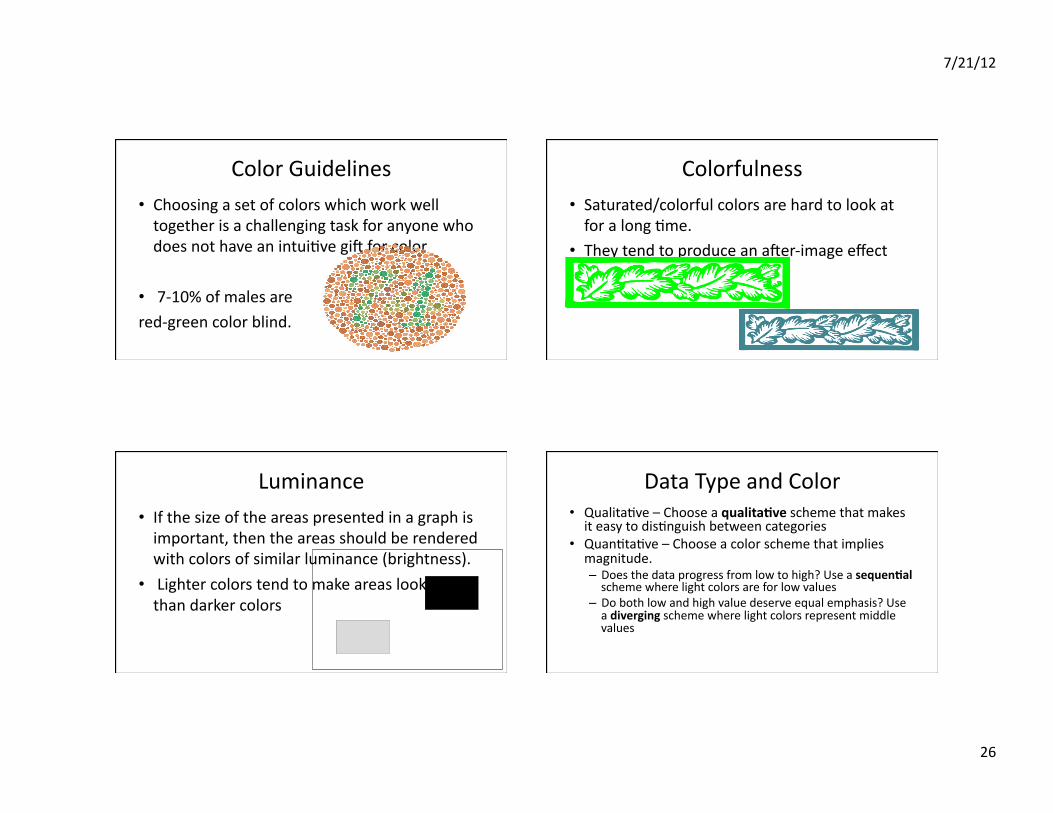
ColorGuidelines• Choosingasetofcolorswhichworkwelltogetherisachallengingtaskforanyonewhodoesnothaveanintui1vegi]forcolor
• 7‐10%ofmalesare
red‐greencolorblind.
Colorfulness• Saturated/colorfulcolorsarehardtolookatforalong1me.
• Theytendtoproduceana]er‐imageeffectwhichcanbedistrac1ng.
Luminance• Ifthesizeoftheareaspresentedinagraphisimportant,thentheareasshouldberenderedwithcolorsofsimilarluminance(brightness).
• Lightercolorstendtomakeareaslooklargerthandarkercolors
DataTypeandColor• Qualita1ve–Chooseaqualita6veschemethatmakesiteasytodis1nguishbetweencategories
• Quan1ta1ve–Chooseacolorschemethatimpliesmagnitude.– Doesthedataprogressfromlowtohigh?Useasequen6alschemewherelightcolorsareforlowvalues
– Dobothlowandhighvaluedeserveequalemphasis?Useadivergingschemewherelightcolorsrepresentmiddlevalues

7/21/12
27
Brewer’sQualita1vePaleOe
Accent
Dark2
Paired
Pastel1
Pastel2
Set1
Set2
Set3
Brewer’sDivergingPaleOe
BrBG
PiYG
PRGn
PuOr
RdBu
RdGy
RdYlBu
RdYlGn
Spectral
Brewer’sSequen1alPaleOes
Blues
BuGn
BuPu
GnBu
Greens
Greys
Oranges
OrRd
PuBu
PuBuGn
PuRd
Purples
RdPu
Reds
YlGn
YlGnBu
YlOrBr
YlOrRd
Case:CO2levelsatMaunaLoa
Timeandthehorizontalaxis

7/21/12
28
MaunaLoaVolcano
LargestVolcanoinworld4kmabovesealevelSummit17kmabovebaseOntheIslandofHawaii DataandphotosavailablefromScrippsIns1tuteandNOAA
MaunaLoaObservatory• Farfromanycon1nent,the
airsampledisagoodaverageforthecentralpacific.
• Beinghigh,itisabovetheinversionlayerwherelocaleffectsarepresent.
• MeasurementsofatmosphericCO2since1958–longestcon1nuousrecord
AtmosphericCarbonDioxide• TheincreasingamountofCO2intheatmospherefromtheburningoffossilfuelshasbecomeaseriousenvironmentalconcern.
• UppersafetylimitforatmosphericCO2is350partspermillion
• DoesariseinCO2leadtoariseinworldtemperatures?
TimeSeries–Pairs:(1me,CO2)
1960 1970 1980 1990 2000 2010
320
340
360
380
date
co2
Pointsaretypicallynotthebestwaytoplot1meseries
7/21/12
29
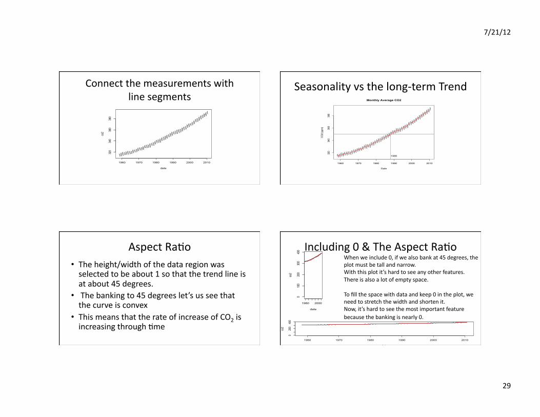
Connectthemeasurementswithlinesegments
1960 1970 1980 1990 2000 2010
320
340
360
380
date
co2
Seasonalityvsthelong‐termTrend
1960 1970 1980 1990 2000 2010
320
340
360
380
Monthly Average CO2
Date
CO
2 (p
pm)
1988
AspectRa1o• Theheight/widthofthedataregionwasselectedtobeabout1sothatthetrendlineisatabout45degrees.
• Thebankingto45degreeslet’susseethatthecurveisconvex
• ThismeansthattherateofincreaseofCO2isincreasingthrough1me
Including0&TheAspectRa1o
1960 2000
0100
200
300
400
date
co2
1960 1970 1980 1990 2000 2010
0200
400
date
co2
Whenweinclude0,ifwealsobankat45degrees,theplotmustbetallandnarrow.Withthisplotit’shardtoseeanyotherfeatures.Thereisalsoalotofemptyspace.Tofillthespacewithdataandkeep0intheplot,weneedtostretchthewidthandshortenit.Now,it’shardtoseethemostimportantfeaturebecausethebankingisnearly0.

7/21/12
30
Resources• TheElementsofGraphingData,Cleveland• VisualRevela8ons,Wainer
• TheVisualDisplayofQuan8ta8veInforma8on,Tu]e
ThankYou