Embed Size (px)
Citation preview
American Economic Review 2020, 110(9): 2748–2782 https://doi.org/10.1257/aer.20181219
2748
*Bordalo: Oxford Said Business School (email: [email protected]); Gennaioli: Università Bocconiand IGiER (email: [email protected]); Ma: Chicago Booth (email: [email protected]);Shleifer: Harvard University (email: [email protected]). Emi Nakamura was the coeditor for this article. We thank five referees for very helpful comments. We thank Olivier Coibion, Xavier Gabaix, Yuriy Gorodnichenko, Luigi Guiso, Lars Hansen, David Laibson, Jesse Shapiro, Paolo Surico, participants at the 2018 AEA meeting, NBER Behavioral Finance, Behavioral Macro, and EF&G Meetings, and seminar participants at Bonn, EIEF, Ecole Politechnique, Harvard, MIT, and LBS for helpful comments. We owe special thanks to Marios Angeletos for several discussions and insightful comments on the paper. We acknowledge the financial support of the Behavioral Finance and Finance Stability Initiative at Harvard Business School and the Pershing Square Venture Fund for Research on the Foundations of Human Behavior. Gennaioli thanks the European Research Council for Financial Support under the ERC Consolidator Grant (GA 647782). We thank Johan Cassell, Bianca He, Francesca Miserocchi, Johnny Tang, and especially Spencer Kwon and Weijie Zhang for outstanding research assistance.
† Go to https://doi.org/10.1257/aer.20181219 to visit the article page for additional materials and author disclosure statements.
Overreaction in Macroeconomic Expectations†
By Pedro Bordalo, Nicola Gennaioli, Yueran Ma, and Andrei Shleifer*
We study the rationality of individual and consensus forecasts of macroeconomic and financial variables using the methodology of Coibion and Gorodnichenko (2015), who examine predictability offorecast errors from forecast revisions. We find that individual fore-casters typically overreact to news, while consensus forecasts under-react relative to full-information rational expectations. We reconcile these findings within a diagnostic expectations version of a dispersed information learning model. Structural estimation indicates that departures from Bayesian updating in the form of diagnostic over-reaction capture important variation in forecast biases across differ-ent series, yielding a belief distortion parameter similar to estimates obtained in other settings. (JEL C53, D83, D84, E13, E17, E27, E47)
According to the rational expectations hypothesis, individuals form beliefs about the future, and make decisions, using statistically optimal forecasts based on their information. A growing body of work tests this hypothesis using survey data on the expectations of households, firm managers, financial analysts, and profes-sional forecasters. The evidence points to systematic predictability of forecast errors. Such predictability has been documented for inflation and other macro forecasts (Coibion and Gorodnichenko 2012, 2015—henceforth, CG; Fuhrer 2019), the aggre-gate stock market (Bacchetta, Mertens, and Wincoop 2009; Amromin and Sharpe2014; Greenwood and Shleifer 2014; Adam, Marcet, and Beutel 2017), the crosssection of stock returns (La Porta 1996; Bordalo, Gennaioli, La Porta, and Shleifer2019—henceforth, BGLS), credit spreads (Greenwood and Hanson 2013, Bordalo,Gennaioli, and Shleifer 2018—henceforth, BGS), short-term interest rates (Cieslak2018), and corporate earnings (De Bondt and Thaler 1985; Ben-David, Graham, andHarvey 2013; Gennaioli, Ma, and Shleifer 2016; Bouchaud et al. 2019). Predictable

2749BORDALO ET AL.: OVERREACTION IN MACROECONOMIC EXPECTATIONSVOL. 110 NO. 9
forecast errors also obtain in controlled experiments (Hommes et al. 2004; Beshears et al. 2013; Frydman and Nave 2016; Landier, Ma, and Thesmar 2019).
What does predictability of forecast errors teach us about how market partici-pants form expectations? A valuable strategy introduced by CG (2015) is to com-pute the correlation between the current forecast revision and the future forecast error, defined as the realization minus the current forecast. Under full-information rational expectations (FIRE) the forecast error is unpredictable, and this correlation should be zero. When this correlation is positive, upward revisions predict higher realizations relative to the forecasts, meaning that the forecast underreacts to infor-mation relative to FIRE. When this correlation is negative, upward forecast revisions predict lower realizations relative to the forecasts, meaning that the forecast overre-acts relative to FIRE.
This test of departures from FIRE can be applied to consensus forecasts. CG (2015) consider consensus forecasts of inflation and other macro variables and find evidence of underreaction relative to FIRE. They interpret this finding as a depar-ture from full information, stemming from information frictions such as rational inattention (Sims 2003, Woodford 2003, Carroll 2003, Mankiw and Reis 2002, Gabaix 2014), while maintaining individual rationality in the form of Bayesian updating. Other empirical findings using consensus forecasts, however, cannot be explained using this account. For instance, upward consensus forecast revisions of firms’ long-term earnings growth predict future disappointment and lower stock returns (BGLS 2019). This evidence points to overreaction of consensus forecasts, in line with the well-known excess volatility of asset prices in finance (Shiller 1981, De Bondt and Thaler 1985, Giglio and Kelly 2018, Augenblick and Lazarus 2018).
CG’s (2015) test of departures from FIRE can also be applied to individual forecasts. D’Arienzo (2019) finds that individual analysts’ forecasts of long-term interest rates overreact. BGLS (2019) also find overreaction for individual analyst expectations of long-term corporate earnings growth. On the other hand, Bouchaud et al. (2019) document underreaction of individual analyst forecasts of firms’ short-term (one year ahead) earnings growth.
This evidence is somewhat unsettling. To some it may suggest that there is no way of thinking systematically about the predictability of forecast errors, confirming the dictum that when one abandons rationality, “anything goes.” This paper shows that this is not the case. First, we show that different tests are informative about different departures from FIRE. Tests of individual beliefs are informative about departures from rationality. Tests of consensus forecasts yield additional information about the role of information frictions. Second, the seemingly contradictory findings can be in good part, though not fully, reconciled, by combining standard information frictions with a deeper departure from Bayesian updating in the direction of overreaction to news. We document this finding by studying expectations for a large set of macro and financial variables at the individual level.
We then offer a theory of individual overreaction based on diagnostic expectations (BGS 2018), a psychologically founded non-Bayesian model of belief formation. In this model, individual expectations overreact to news. At the same time, we follow Woodford (2003) and CG (2015) in assuming that information is dispersed across individuals. We show that this model can qualitatively and quantitatively unify many

2750 THE AMERICAN ECONOMIC REVIEW SEPTEMBER 2020
patterns in the data, including individual overreaction and consensus underreaction to news in most cases.
We use both the Survey of Professional Forecasters (SPF) and the Blue Chip Survey (Blue Chip), which gives us 22 expectations series in total (four variables appear in both surveys), including forecasts of real economic activity, consumption, investment, unemployment, housing starts, government expenditures, and multiple interest rates. SPF data are publicly available; Blue Chip data were purchased and hand coded for the earlier part of the sample. This data expands the sources and variables analyzed by CG (2015). We report five principal findings.
First, the rational expectations hypothesis is consistently rejected in individual forecast data. Individual forecast errors are systematically predictable from forecast revisions.
Second, overreaction to information is the norm in individual forecast data, mean-ing that upward revisions are associated with realizations below forecasts. In only a few series we find individual forecaster-level underreaction.
Third, for consensus forecasts, we generally find the opposite pattern of underre-action, which confirms, using our expanded dataset, the CG finding of informational rigidity.
Fourth, a model of belief formation that we call diagnostic expectations (BGS 2018) can be used to organize the evidence. The model incorporates Kahneman and Tversky’s (1972) representativeness heuristic, formalized as in Gennaioli and Shleifer (2010) and Bordalo et al. (2016)—henceforth, BCGS, into a frame-work of learning from noisy private signals.1 In this model, belief distortions follow the “kernel of truth”: each forecaster overweighs the probability of states that have become truly more likely in light of his noisy signal. The degree of overweighting is controlled by the diagnosticity parameter θ . When θ = 0 , our model reduces to the CG model of information frictions, in which consensus forecasts underreact but individual-level forecasts are rational (i.e., their errors are unpredictable). When θ > 0 , the model departs from Bayesian updating in the direction of overreaction. This departure allows us to reconcile positive consen-sus-level and negative individual-level CG coefficients. Intuitively, when θ > 0 each individual forecaster overreacts to his noisy signal, so the individual CG coef-ficient is negative but still does not react at all to the signals of other forecasters, potentially creating a positive consensus CG coefficient.
Fifth, our model has additional predictions that we check with a structural esti-mation exercise. In particular, our model implies that whether the consensus fore-cast over- or underreacts, and the strength of individual-level overreaction, should depend on the characteristics of the data-generating process, such as its persistence and volatility. We estimate the parameters of each series’ data-generating process and recover latent parameters such as the degree of diagnosticity θ and the noise in forecasters’ information using the simulated method of moments. To probe the robustness of our findings, we try three different estimation methods, which yield the following robust results. First, the diagnostic parameter θ is on average around
1 Gennaioli and Shleifer (2010) proposed this model to account for lab experiments on probabilistic judgments, and BCGS (2016) applied it to social stereotypes. The model has then been used to account for credit cycles (BGS 2018) and the cross section of stock returns (BGLS 2019).

2751BORDALO ET AL.: OVERREACTION IN MACROECONOMIC EXPECTATIONSVOL. 110 NO. 9
0.5, which lies in the ballpark of estimates obtained in other contexts using different data and methods (BGS 2018, BGLS 2019). The resulting distortions in beliefs are considerable: θ = 0.5 means that forecasts react to news 50 percent more than do rational expectations. Second, in line with our model, more persistent series exhibit weaker overreaction than less persistent ones. Finally, due to differences in per-sistence and volatility between series, our model captures about half of the variation in the consensus forecast rigidity among them. Allowing the diagnostic parameter to vary between series allows the model to explain most of the cross-series variation.
The paper proceeds as follows. After describing the data in Section I, we docu-ment in Section II the prevalence of both forecaster-level overreaction to informa-tion and consensus-level rigidity. We then perform robustness checks with respect to a number of potential concerns, including forecaster heterogeneity, small sam-ple bias, measurement error, nonstandard loss functions, and the non-normality of shocks. In Section III we introduce the model and show that it helps reconcile con-sensus- and individual-level predictability of forecast errors. In Section IV we esti-mate the model. In Section V we take stock and lay out some key next steps for the fast-growing work on departures from rational expectations.
Our main empirical contribution is to carry out a systematic analysis of mac-roeconomic and financial forecasts and offer a reconciliation for the seemingly contradictory patterns discussed at the outset. As we shall see, unification is not complete: we cannot account for individual-level underreaction to news, which we document for short-term interest rates and has also been documented by Bouchaud et al. (2019) for short-term earnings forecasts. We suggest in Section V that the ker-nel of truth logic offers a promising approach to reconciling these findings as well.
Our analysis also relates to other modeling approaches to expectation errors. For example, with natural expectations (Fuster, Laibson, and Mendel 2010), fore-casters neglect longer lags, causing overreaction to short-term changes. While our model shares some predictions with natural expectations, it makes distinctive pre-dictions, such as overreaction to longer lags, that we show more closely describe the data.2 Overconfidence, in the sense of overestimating the precision of private news, also implies an exaggerated reaction to private signals (Daniel, Hirshleifer, and Subrahmanyam 1998; Moore and Healy 2008). In independent and insightful work, Broer and Kohlhas (2018) document individual overreaction in forecasts for GDP and inflation and consider overconfidence as the reason. In a similar vein, ear-lier work by Benigno and Karantounias (2019) uses overconfidence to rationalize the volatility of individual prices and the rigidity of aggregate prices. We find that diagnostic expectations can better explain several features of the data documented here and elsewhere, such as instances of consensus overreaction, individual-level overreaction to the signals the forecaster attends to (which include salient public signals), and systematic differences across series.
In our view, diagnostic expectations offer a theoretically tractable, empirically plausible, and parsimonious departure from rational expectations. They explain
2 Incentives may distort professional forecasters’ stated expectations. Ottaviani and Sørensen (2006) point out that if forecasters compete in an accuracy contest with winner-take-all rules, they overweigh private information. In contrast, Fuhrer (2019) argues that in the SPF data, individual forecast revisions can be negatively predicted from past deviations relative to consensus. Kohlhas and Walther (2018) also offer a model of asymmetric loss functions. We discuss these possibilities later in the paper.

2752 THE AMERICAN ECONOMIC REVIEW SEPTEMBER 2020
puzzling features of the data and can be incorporated into quantitative models in macroeconomics and finance. More work is needed to find the best formulation, but existing estimates of the critical diagnosticity parameter can be used as a starting point in such an analysis (Bordalo, Gennaioli, Shleifer, and Terry 2019).
I. The Data
Data on Forecasts.—We collect forecast data from two sources: SPF and Blue Chip.3 SPF is a survey of professional forecasters currently run by the Federal Reserve Bank of Philadelphia (SPF 1968–2016). At a given point in time, around 40 forecasters contribute to SPF anonymously. SPF is conducted on a quarterly basis, around the end of the second month in the quarter. It provides both consensus forecast data and forecaster-level data. In SPF, individual forecasters are anony-mous and identified by forecaster IDs. Forecasters report forecasts for outcomes in the current and next four quarters, typically about the level of the variable in each quarter.
Blue Chip is a survey of panelists from around 40 major financial institutions (Blue Chip Publications 1983–2016). The names of institutions and forecasters are disclosed. The survey is conducted around the beginning of each month. To match with the SPF timing, we use Blue Chip forecasts from the end-of-quarter month survey (i.e., March, June, September, and December). Blue Chip has con-sensus forecasts available electronically, and we digitize individual-level forecasts from PDF publications. Panelists forecast outcomes in the current and next four to five quarters. For variables such as GDP, they report (annualized) quarterly growth rates. For variables such as interest rates, they report the quarterly average level.
For both SPF and Blue Chip, the median (mean) duration of a panelist contrib-uting forecasts is about 16 (23) quarters. Thus for each variable, we have an unbal-anced panel. Given the timing of the SPF and Blue Chip forecasts we use, by the time the forecasts are made in quarter t (i.e., around the end of the second month in quarter t ), forecasters know the actual values of variables with quarterly releases (e.g., GDP) up to quarter t − 1 and the actual values of variables with monthly releases (e.g., unemployment rate) up to the previous month.
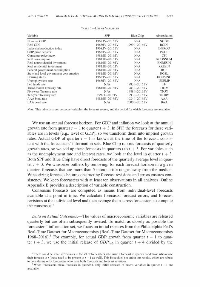
Table 1 presents the list of variables we study as well as the time range for which forecast data are available from SPF and/or Blue Chip. These variables cover both macroeconomic outcomes—such as GDP, price indices, consumption, investment, unemployment, government consumption—and financial variables, primarily yields on government bonds and corporate bonds. SPF covers most of the macro variables and selected interest rates (three-month Treasuries, ten-year Treasuries, and AAA corporate bonds). Blue Chip includes real GDP and a larger set of interest rates (fed funds, three-month, five-year, and ten-year Treasuries, AAA as well as BAA corpo-rate bonds). Relative to CG (2015), we add two SPF variables (nominal GDP and the ten-year Treasury rate) as well as the Blue Chip forecasts.
3 Blue Chip provides two sets of forecast data: Blue Chip Economic Indicators (BCEI) and Blue Chip Financial Forecasts (BCFF). We do not use BCEI since historical forecaster-level data are only available for BCFF.
2753BORDALO ET AL.: OVERREACTION IN MACROECONOMIC EXPECTATIONSVOL. 110 NO. 9
We use an annual forecast horizon. For GDP and inflation we look at the annual growth rate from quarter t − 1 to quarter t + 3 . In SPF, the forecasts for these vari-ables are in levels (e.g., level of GDP), so we transform them into implied growth rates. Actual GDP of quarter t − 1 is known at the time of the forecast, consis-tent with the forecasters’ information sets. Blue Chip reports forecasts of quarterly growth rates, so we add up these forecasts in quarters t to t + 3 . For variables such as the unemployment rate and interest rates, we look at the level in quarter t + 3 . Both SPF and Blue Chip have direct forecasts of the quarterly average level in quar-ter t + 3 . We winsorize outliers by removing, for each forecast horizon in a given quarter, forecasts that are more than 5 interquartile ranges away from the median. Winsorizing forecasts before constructing forecast revisions and errors ensures con-sistency. We keep forecasters with at least ten observations in all analyses. Online Appendix B provides a description of variable construction.
Consensus forecasts are computed as means from individual-level forecasts available at a point in time. We calculate forecasts, forecast errors, and forecast revisions at the individual level and then average them across forecasters to compute the consensus.4
Data on Actual Outcomes.—The values of macroeconomic variables are released quarterly but are often subsequently revised. To match as closely as possible the forecasters’ information set, we focus on initial releases from the Philadelphia Fed’s Real-Time Dataset for Macroeconomists ( Real-Time Dataset for Macroeconomists 1968–2016).5 For example, for actual GDP growth from quarter t − 1 to quar-ter t + 3 , we use the initial release of GD P t+3 in quarter t + 4 divided by the
4 There could be small differences in the set of forecasters who issue a forecast in quarter t and those who revise their forecast at t (these need to be present at t − 1 as well). This issue does not affect our results, which are robust to considering only forecasters who have both forecasts and forecast revisions.
5 When forecasters make forecasts in quarter t, only initial releases of macro variables in quarter t − 1 are available.
Table 1—List of Variables
Variable SPF Blue Chip Abbreviation
Nominal GDP 1968:IV–2016:IV N/A NGDPReal GDP 1968:IV–2016:IV 1999:I–2016:IV RGDPIndustrial production index 1968:IV–2016:IV N/A INPRODGDP price deflator 1968:IV–2016:IV N/A PGDPConsumer price index 1981:III–2016:IV N/A CPIReal consumption 1981:III–2016:IV N/A RCONSUMReal nonresidential investment 1981:III–2016:IV N/A RNRESINReal residential investment 1981:III–2016:IV N/A RRESINFederal government consumption 1981:III–2016:IV N/A RGFState and local government consumption 1981:III–2016:IV N/A RGSLHousing starts 1968:IV–2016:IV N/A HOUSINGUnemployment rate 1968:IV–2016:IV N/A UNEMPFed funds rate N/A 1983:I–2016:IV FFThree-month Treasury rate 1981:III–2016:IV 1983:I–2016:IV TB3MFive-year Treasury rate N/A 1988:I–2016:IV TN5YTen-year Treasury rate 1992:I–2016:IV 1993:I–2016:IV TN10YAAA bond rate 1981:III–2016:IV 1984:I–2016:IV AAABAA bond rate N/A 2000:I–2016:IV BAA
Note: This table lists our outcome variables, the forecast source, and the period for which forecasts are available.

2754 THE AMERICAN ECONOMIC REVIEW SEPTEMBER 2020
contemporaneous release of GD P t−1 . We perform robustness checks using other vin-tages of actual outcomes including the latest release. For financial variables, the actual outcomes are available daily and are permanent (not revised). We use historical data from the Federal Reserve Bank of St. Louis. In addition, we always study the prop-erties of the actuals (mean, standard deviation, persistence, etc.) using the same time periods as the corresponding forecasts. The same variable from SPF and Blue Chip may have slightly different actuals when the two datasets cover different time periods.
Summary Statistics.—We present summary statistics of average forecasts and corresponding actuals in online Appendix C Table C1. Here we present summary statistics of forecast errors and revisions. Table 2 shows the consensus forecast errors and revisions at a horizon of quarter t + 3 as well as the dispersion of indi-vidual forecasts. The table also shows statistics for the quarterly share of forecasters with no meaningful revisions6 and a measure of the dispersion in revisions, namely the probability that less than 80 percent of forecasters revise in the same direction.
Several patterns emerge from Table 2. First, the consensus forecast error is sta-tistically indistinguishable from zero for most variables. The main exceptions are interest rates, for which consensus forecasts are systematically above realizations. This is likely due to the fact that interest rates declined secularly during our sample period, while forecasters adjusted only partially to the trend. Second, there is signif-icant dispersion of forecasts and revisions at each point in time. Third, the share of nonrevising forecasters is small, and revisions go in different directions. As the final column shows, it is uncommon to have quarters where more than 80 percent of fore-casters revise in the same direction. This suggests that different forecasters observe or attend to different news, either because they are exposed to different information or because they use different models, or both.
II. Properties of Individual and Consensus Forecasts
Many tests of the rational expectations hypothesis assess whether forecast errors can be predicted using information available at the time the forecast is made. Understanding whether departures from rational expectations are due to over- or underreaction to information is more challenging, since the forecaster’s full infor-mation set is not directly observed by the econometrician. To do so, we build on the method developed by CG (2015), which tests whether errors of consensus forecasts are predictable from revisions of consensus forecasts, assuming that revisions mea-sure the reaction to available news.
While the CG test was originally developed to assess whether consensus fore-casts underreact, or are rigid, relative to the FIRE benchmark, it can be used as an empirical test on any expectations panel data for which forecast revisions can be computed. We first describe the general structure of the test and then discuss its implementation and interpretation using data on the individual level as well as con-sensus forecasts.
6 We categorize a forecaster as making no revision if he provides nonmissing forecasts in both quarters t − 1 and t and the forecasts change by less than 0.01 percentage points. For variables in rates, the data is often rounded to the first decimal point, and this rounding may lead to a higher incidence of no revision.

2755BORDALO ET AL.: OVERREACTION IN MACROECONOMIC EXPECTATIONSVOL. 110 NO. 9
Starting with the original setting in CG (2015), denote by x t+h | t the consen-sus forecast made at time t about the future value x t+h of a variable. That is, x t+h | t = (1/I ) ∑ i x t+h | t i , where x t+h | t i is the forecast of individual i and I > 1 is the number of forecasters. Denote by x t+h | t−1 the forecast of the same variable in the previous period. The h -periods-ahead forecast revision at t is given by F R t,h = ( x t+h | t − x t+h | t−1 ) , or the one-period change in the forecast about x t+h . The pre-dictability of forecast errors is then assessed by estimating the regression,
(1) x t+h − x t+h | t = β 0 + β 1 F R t,h + ϵ t,t+h .
If forecast errors are not predictable from forecast revisions, then β 1 = 0 . This should hold under FIRE, where each forecaster is rational and all forecast-ers share the same, full-information set. In this case, all forecasters provide the
Table 2—Summary Statistics
Consensus Individual
Errors Revisions Forecast
dispersion
Nonrev share
Pr(<80% revise same direction)Mean SD SE Mean SD
Variable (1) (2) (3) (4) (5) (6) (7) (8)
Nominal GDP (SPF) −0.30 1.73 0.20 −0.16 0.71 1.00 0.02 0.77Real GDP (SPF) −0.23 1.71 0.20 −0.18 0.62 0.79 0.02 0.74Real GDP (BC) −0.07 1.28 0.19 −0.12 0.47 0.38 0.05 0.64GDP price index (SPF) −0.06 1.14 0.15 0.01 0.44 0.62 0.05 0.78CPI (SPF) −0.26 1.07 0.14 −0.12 0.47 0.53 0.07 0.70Real consumption (SPF) 0.35 1.13 0.16 −0.07 0.44 0.60 0.03 0.77Industrial production (SPF) −1.06 3.85 0.43 −0.34 1.09 1.57 0.07 0.76Real nonresidential investment (SPF)
0.22 5.79 0.82 −0.29 1.80 2.21 0.02 0.72
Real residential investment (SPF) −0.06 8.35 1.21 −0.66 2.42 4.02 0.03 0.84Real federal government consumption (SPF)
0.02 3.19 0.41 0.10 1.19 1.93 0.07 0.88
Real state and local government consumption (SPF)
0.04 1.14 0.16 −0.05 0.35 0.92 0.11 0.90
Housing start (SPF) −3.43 18.38 2.35 −2.24 6.04 8.35 0.00 0.66Unemployment (SPF) 0.00 0.76 0.09 0.05 0.32 0.29 0.18 0.78Fed funds rate (BC) −0.41 1.01 0.15 −0.18 0.53 0.45 0.23 0.70Three-month Treasury rate (SPF) −0.54 1.17 0.16 −0.20 0.52 0.45 0.15 0.69Three-month Treasury rate (BC) −0.52 1.01 0.15 −0.19 0.50 0.45 0.17 0.68Five-year Treasury rate (BC) −0.42 0.87 0.13 −0.16 0.45 0.40 0.12 0.62Ten-year Treasury rate (SPF) −0.49 0.74 0.11 −0.13 0.37 0.37 0.10 0.61Ten-year Treasury rate (BC) −0.44 0.74 0.11 −0.14 0.39 0.34 0.13 0.54AAA corporate bond rate (SPF) −0.47 0.85 0.11 −0.12 0.39 0.50 0.08 0.72AAA corporate bond rate (BC) −0.43 0.69 0.10 −0.13 0.36 0.45 0.12 0.70BAA corporate bond rate (BC) −0.46 0.66 0.12 −0.15 0.31 0.40 0.12 0.77
Notes: Columns 1 to 5 show statistics for errors and revisions of consensus (average) forecasts. Errors are actuals minus forecasts, and actuals are realized outcomes corresponding to the forecasts. Standard errors of forecast errors are calculated with Newey and West (1994) standard errors. Revisions are forecasts of the outcome made in quar-ter t minus forecasts of the same outcome made in quarter t − 1 . Columns 6 to 8 show statistics of individual-level forecasts. The forecast dispersion column shows the mean of quarterly standard deviations of individual-level fore-casts. Nonrevisions are instances where forecasts are available in both quarter t and quarter t − 1 and the change in the value is less than 0.01 percentage points. The nonrevision column shows the mean of quarterly nonrevision shares. The final column shows the fraction of quarters where less than 80 percent of the forecasters revise in the same direction. All values are in percentages. The format for nominal GDP to housing start is the growth rate from the end of quarter t − 1 to the end of quarter t + 3 . The format for unemployment rate to BAA corporate bond rate is the average level in quarter t + 3 .
2756 THE AMERICAN ECONOMIC REVIEW SEPTEMBER 2020
same rational forecast, and forecast errors should have no predictability. On the other hand, a positive coefficient β 1 implies that when the average fore-cast revision is positive, F R t,h > 0 , the consensus forecast is not optimistic enough; similarly, when the average forecast revision is negative, F R t,h < 0 , the consensus forecast is not pessimistic enough . Thus β 1 > 0 indicates underre-action of consensus forecasts relative to FIRE. By the same logic, β 1 < 0 indicates overreaction of consensus forecasts relative to FIRE .
CG (2015) find β 1 > 0 for inflation expectations.7 This finding rejects FIRE but not rational expectations as such. Indeed, CG show that β 1 > 0 can be obtained in models that only relax the full-information assumption, while individual forecasters rationally update their forecasts based on noisy private signals. Maintaining ratio-nality of updating, however, is not without consequences. It implies, in particular, that at the individual level forecast errors should remain unpredictable. To assess rationality, and to learn how forecasters update, we must perform the error predict-ability test at the individual level.
To analyze forecast error predictability at the individual level, we adapt test (1) using two different methods. Using individual forecast revisions F R t,h i = ( x t+h | t i − x t+h | t−1 i ) and forecast errors x t+h − x t+h | t i , we first pool forecast-ers and estimate a common coefficient β 1
p from the regression,
(2) x t+h − x t+h | t i = β 0 p + β 1
p F R t,h i + ϵ t,t+h i .
Superscript p on the coefficients refers to the pooling of individual-level data. Note that β 1
p > 0 indicates that the average forecaster underreacts to his own informa-tion, while β 1
p < 0 indicates that the average forecaster overreacts. Rational expec-tations imply that, even with information frictions, β 1
p = 0 .The second method is to run forecaster-by-forecaster regressions,
(3) x t+h − x t+h | t i = β 0 i + β 1 i F R t,h i + v t,t+h i , i = 1, …, I ,
which yields a distribution of individual coefficients β 1 i , i = 1, …, I . We can then take the median coefficient as indicative of whether the majority of forecasters over- or underreacts. Again, rational expectations imply β 1 i = 0 for all i .
The forecaster-by-forecaster specification in (3) has two main advantages. First, it does not impose the restriction of a common coefficient β 1
p . Second, it controls for persistent individual-level differences in forecaster optimism (e.g., due to different priors). Heterogeneity of this type may create a bias toward underreaction in the pooled data. Specifically, optimistic forecasters tend to make negative errors and receive bad news and thus make negative revisions, leading to a spurious positive correlation between forecast revisions and forecast errors. On the other hand, the forecaster-by-forecaster specification has the shortcoming that there are a limited
7 Specifically, CG (2015) estimate equation (1) for the consensus forecast of the GDP price deflator (PGDP_SPF) at a horizon h = 3 and find β 1 = 1.2 , which is robust to a number of controls. They also run equa-tion (1) for 13 SPF variables by pooling forecast horizons from h = 0 to h = 3 and find qualitatively similar results, with 8 out of 13 variables exhibiting significantly positive β 1 values and the average coefficient being close to 0.7 (see Figure 1, panel B of CG 2015). The general message is that consensus forecasts of macroeconomic variables exhibit rigidity.

2757BORDALO ET AL.: OVERREACTION IN MACROECONOMIC EXPECTATIONSVOL. 110 NO. 9
number of observations for each forecaster for each series, which decreases statisti-cal power and makes it difficult to reliably estimate β 1 i .
What does CG’s (2015) general message that consensus forecasts of macroeco-nomic variables exhibit rigidity imply for the updating of individual forecasters? As mentioned above, rigidity of the consensus ( β 1 > 0 ) rejects FIRE and is consistent with information frictions. However, it does not exclude the coexistence of these frictions with violations of rationality ( β 1
p ≠ 0, β 1 i ≠ 0 ) in the form of over- or underreaction. In particular, β 1 > 0 is also consistent with no information rigid-ity at all and predictability being entirely driven by individual-level underreaction ( β 1 = β 1
p > 0 ). Without looking at individual forecasts, there is no way to tell how forecasters update and which mechanism fits the data best.
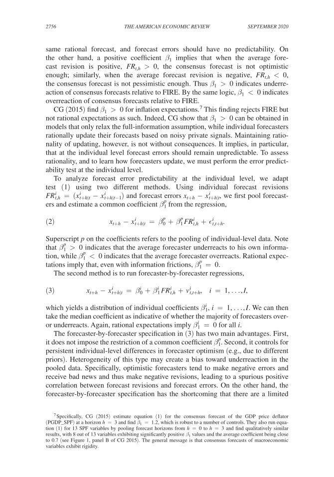
Figure 1 plots the estimates of equations (1) and (2), and Table 3 shows the point estimates, standard errors, and p-values. For consensus forecasts, the diamonds in Figure 1 and columns 1 to 3 in Table 3 show results for the coefficient β 1 in equa-tion (1), for our 22 series and the same baseline horizon h = 3 . The standard errors are Newey–West with the automatic bandwidth selection following Newey and West (1994). The estimated β 1 is positive for 17 out of 22 series, statistically significant for 9 of them at the 5 percent confidence level and for a further 3 series at the 10 percent level. Our point estimate for inflation forecasts coincides with CG’s. While results for the other SPF series are not directly comparable (since CG pool across forecast horizons), the estimates lie in a similar range. The one exception is the consensus forecast of RGF_SPF (federal government spending), which displays strong overreaction. Results from the Blue Chip survey align well with SPF where they overlap but do not exhibit significant consensus predictability for the remaining financial series.
Figure 1. Forecast Error on Forecast Revision (CG) Regression Results
Notes: This figure plots the forecast error on forecast revision regression coefficients. The diamonds represent the coefficient β 1 in equation (1) using consensus forecasts, and the circles represent the coefficient β 1
p in equation (2) using individual forecasts. Standard errors are Newey-West for consensus time series regressions and clustered by forecaster and time for pooled individual-level panel regressions.
−1
0
1
2
NGDP_SPF
RGDP_SPF
RGDP_BC
INDPROD_S
PF
PGDP_SPF
CPI_SPF
RCONSUM_S
PF
RNRESIN_S
PF
RRESINV_S
PF
RGF_SPF
RGSL_SPF
UNEMP_S
PF
HOUSING_S
PF
FF_BC
TB3M_S
PF
TB3M_B
C
TN5Y_B
C
TN10Y_S
PF
TN10Y_B
C
AAA_SPF
AAA_BC
BAA_BC
Consensus CG coefficients Individual CG coefficients

2758 THE AMERICAN ECONOMIC REVIEW SEPTEMBER 2020
For the individual-level forecasts, the circles in Figure 1 and columns 4 to 7 in Table 3 show results for the coefficient β 1
p in equation (2), using pooled individual-level regressions, for our 22 series and the same baseline horizon h = 3 . The results are essentially reversed from those using consensus forecasts: at the indi-vidual level, the average forecaster appears to mostly overreact to information, as reflected by a negative β 1
p coefficient. The estimated β 1 p is negative for 14 out of the 22
series (12 out of 18 variables) and significantly negative for 8 series at the 5 percent confidence level and for 4 other series at the 10 percent level. Except for short-term interest rates (fed funds and 3-month T-bill rate), all financial variables display overreaction. But many macro variables also display individual-level overreaction, including nominal GDP, real GDP (in SPF, not in Blue Chip), industrial production, CPI, real consumption, real federal government expenditures, and real state and local government expenditures. Estimates for the fed funds rate, three-month T-bill rate, and unemployment rate display individual-level underreaction with positive and sta-tistically significant β 1
p . GDP price deflator inflation, real GDP in Blue Chip, and nonresidential investment display neither over- nor underreaction ( β 1
p close to zero).To account for persistent differences among forecasters such as those stemming
from priors, Table C2 in online Appendix C also reports regressions with forecaster fixed effects. Now the estimated β 1
p is negative for 16 series and significantly neg-ative for 12 series at the 5 percent confidence level and for 2 other series at the
Table 3— Error-on-Revision Regression Results
Consensus Individual
β 1 SE p-value β 1 p SE p-value Median
Variable (1) (2) (3) (4) (5) (6) (7)
Nominal GDP (SPF) 0.56 0.21 0.01 −0.22 0.07 0.00 −0.20Real GDP (SPF) 0.44 0.23 0.06 −0.15 0.09 0.09 −0.08Real GDP (BC) 0.57 0.33 0.08 0.11 0.19 0.58 −0.03GDP price index inflation (SPF) 1.41 0.21 0.00 0.18 0.13 0.18 −0.11CPI (SPF) 0.29 0.22 0.17 −0.19 0.12 0.10 −0.25Real consumption (SPF) 0.24 0.25 0.33 −0.24 0.11 0.02 −0.26Industrial production (SPF) 0.71 0.30 0.02 −0.16 0.09 0.09 −0.19Real nonresidential investment (SPF) 1.06 0.36 0.00 0.08 0.15 0.60 0.09Real residential investment (SPF) 1.22 0.33 0.00 0.01 0.10 0.92 −0.09Real federal government consumption (SPF) −0.43 0.23 0.06 −0.59 0.07 0.00 −0.52Real state and local government consumption (SPF) 0.63 0.34 0.06 −0.43 0.04 0.00 −0.44Housing start (SPF) 0.40 0.29 0.18 −0.23 0.09 0.01 −0.27Unemployment (SPF) 0.82 0.2 0.00 0.34 0.12 0.00 0.23Fed funds rate (BC) 0.61 0.23 0.01 0.20 0.09 0.03 0.22Three-month Treasury rate (SPF) 0.60 0.25 0.01 0.27 0.10 0.01 0.28Three-month Treasury rate (BC) 0.64 0.25 0.01 0.21 0.09 0.02 0.17Five-year Treasury rate (BC) 0.03 0.22 0.88 −0.11 0.10 0.29 −0.17Ten-year Treasury rate (SPF) −0.02 0.27 0.95 −0.19 0.10 0.06 −0.24Ten-year Treasury rate (BC) −0.08 0.24 0.73 −0.18 0.11 0.11 −0.29AAA corporate bond rate (SPF) −0.01 0.23 0.95 −0.22 0.07 0.00 −0.32AAA corporate bond rate (BC) 0.21 0.20 0.29 −0.14 0.06 0.02 −0.27BAA corporate bond rate (BC) −0.18 0.27 0.50 −0.29 0.09 0.00 −0.32
Notes: This table shows coefficients from the CG (forecast error on forecast revision) regression. Columns 1 to 6 show the coefficients of consensus time series regressions and individual-level pooled panel regressions together with standard errors and p-values. Column 7 shows the median coefficients in forecaster-by-forecaster regressions. For consensus time series regressions, standard errors are Newey-West with the automatic bandwidth selection procedure of Newey and West (1994). For individual-level panel regressions, standard errors are clustered by both forecaster and time.

2759BORDALO ET AL.: OVERREACTION IN MACROECONOMIC EXPECTATIONSVOL. 110 NO. 9
10 percent level. Finally, Table 3, column 7 shows the median coefficient from the forecaster-by-forecaster regression of equation (3). In online Appendix C, Table C3, we report confidence intervals of the median coefficient using block bootstrap.8 We resample time periods from the panel using blocks of 20 quarters each (we keep all forecasts made during each block of time period) and compute the median coeffi-cient in 500 bootstrap samples. The results confirm our previous findings from the pooled specification. The median coefficient is negative at the 5 percent confidence level for 13 out of 22 series and is very close to the results of the baseline regression in equation (2) above. The median forecast for short-term interest rates (the fed funds rate and the three-month T-bill rate) again displays underreaction, while that for real GDP, GDP price deflator, and investment displays neither over nor underre-action. Overall, as Figure 1 and Table 3 show, the prevalent finding is overreaction.
The forecast series are not all independent. The CPI index and the GDP deflator are highly correlated, as are the different short-term interest rate series. Nonetheless, a general message emerges from the data. At the consensus level we mostly see informational rigidity, particularly for the macro variables and short-term interest rates. At the individual level, in contrast, we mostly see overreaction, particularly for longer-term interest rates but also for several macro variables. This evidence suggests that a story based entirely on information rigidities cannot fit the data. Departures from rationality are needed.
Robustness Checks.—There are possible concerns that predictability of forecast errors might arise from features of the data unrelated to individuals’ under- or over-reaction to news. We next show that our results are robust to several such confounds.
Limited Duration: We first discuss problems related to limited duration (small T ). Finite-sample biases exist in time series regressions (Kendall 1954, Stambaugh 1999) and panel regressions with fixed effects (Nickell 1981). These finite sam-ple biases are large when the predictor variables are persistent. Because the pre-dictor variable in the CG regressions, the forecast revision, has low persistence in the data (about zero for most variables at the individual level), this issue should be small. Table 3 shows the pooled individual-level panel tests with no individual fixed effects, which are not subject to the Nickell bias (Hjalmarsson 2008). In addi-tion, the results with individual fixed effects (online Appendix C, Table C2) and without fixed effects (Table 3) are similar, which also alleviates the finite-sample concern. For the forecaster-by-forecaster time series regressions, we also perform finite-sample Stambaugh bias-adjusted regressions and report the bias-adjusted median coefficients in online Appendix C, Table C3. The results are very similar to those from the OLS regressions reported in Table 3, column 7.
Measurement Error: We also perform robustness checks for measurement error in both forecasts and actual outcomes. Forecasts measured with noise can mechan-ically lead to negative predictability of forecast errors in individual-level tests: a
8 We have less power to assess the significance of individual coefficients. For most variables, 20–30 percent of forecasters have negative and significant coefficients, while about 5 percent of them have positive and significant coefficients.
2760 THE AMERICAN ECONOMIC REVIEW SEPTEMBER 2020
positive shock increases the measured forecast revision and decreases the forecast error. To address this concern, we regress forecast errors at a certain horizon on fore-cast revisions for a different horizon. To the extent that overreactions are positively correlated for forecasts at different horizons, this specification would still yield a negative coefficient while avoiding the mechanical measurement error problem of overlap in the left- and right-hand-side variables.
We implement this general strategy in two ways. First, in online Appendix C, Table C4 we regress the forecast error at horizon t + 2 , that is ( x t+2 − x t+2 | t i ), on the forecast revision at horizon t + 3 , that is ( x t+3 | t i − x t+3 | t−1 i ) . We find strong neg-ative predictability at the individual level in this specification as well. Second, in Section IIIB and online Appendix E we consider which series are better described by a hump-shaped, AR(2) process than by an AR(1) process. In this context, we regress the forecast error at horizon t + 3, ( x t+3 − x t+3 | t i ), on the forecast revisions for periods t + 2 and t + 1 , ( x t+2 | t i − x t+2 | t−1 i ) and ( x t+1|t i − x t+1|t−1 i ) respectively, with similar results (online Appendix E, Table E2). These findings alleviate con-cerns about measurement error in forecasts.
In addition, we assess the robustness of the results with respect to the measure-ment of the outcome variable. For example, in online Appendix C, Table C5, we measure the outcome variable using its most recent release. The results are similar to those in Table 3.
Finally, in Section IV we estimate our model without using information from the CG coefficients; we obtain estimates that also indicate significant individual-level overreaction and generate CG regression coefficients very similar to the data. These findings assuage measurement error concerns.
Forecaster Incentives and Loss Functions: Another concern is that forecast errors reflect not cognitive limitations but forecasters’ biased incentives. Although a fore-caster’s objective is difficult to observe, we can discuss the implications of several forecaster loss functions proposed in the literature.
With an asymmetric loss function (Capistrán and Timmermann 2009), the over-reaction pattern in Table 3 may be generated by a combination of (i) an asymmetric cost of over- or underpredictions and (ii) time-varying volatility (Pesaran and Weale 2006). One key prediction here is that asymmetric loss functions would generate nonzero average forecast errors. In the data, however, forecasts for most variables are not systematically biased. The average consensus forecast errors are typically small and insignificant (Table 2).9 This is also true for individual forecast errors: we fail to reject that the average error is different from zero for about 60 percent of forecasters for the macroeconomic variables.10
Other types of incentives stem from forecaster reputations. One of them is fore-cast smoothing. In response to news at t , forecasters may wish to minimize forecast revisions by taking into account the previous forecast x t+h | t−1 i as well as the future path x t+h | t+j i . To assess the relevance of this mechanism, note that forecast smoothing
9 As we already discussed, the only exception is interest rate variables, but here the systematic average error is most likely due to the downward trend in interest rates, not to asymmetric loss functions. There is no reason to expect forecasters’ loss functions to be asymmetric for interest rates but not for macro variables.
10 Some individual forecasters have average errors that are significantly different from zero for some series, but these average out in the population for nearly all series.

2761BORDALO ET AL.: OVERREACTION IN MACROECONOMIC EXPECTATIONSVOL. 110 NO. 9
should reduce the current revision for the current quarter ( h = 0 ), creating under-reaction. This prediction is contradicted by the data: negative predictability prevails even at this horizon (online Appendix C, Table C6).
Reputational mechanisms may also create strategic interactions among forecast-ers, again leading to predictable individual-level forecast errors. On the one hand, individuals may wish to stay close to consensus forecasts (Morris and Shin 2002, Fuhrer 2019). Let x ̃ t+h | t i = α x t+h | t i + (1 − α) x ̃ t+h | t , where x t+h | t i is the individual rational forecast and x ̃ t+h | t is the average contemporaneous forecast with this bias (which coincides with the consensus without this bias). Our benchmark model has α = 1 , but for α < 1 forecasters put weight on others’ signals at the expense of their own. This force causes individual forecasts to be strategic complements. As a result, it causes individual-level underreaction, or positive individual-level CG coef-ficients, contrary to our findings.11
In online Appendix C, Table C7 we address this mechanism by controlling in the pooled specification of equation (2) for the deviation of the forecast in quarter t − 1 from the consensus ( x t+h|t−1 i − x t+h|t ) . The consensus is released between quarter t − 1 and quarter t , so controlling for the deviation takes into account potential news and adjustments related to the release of the consensus. The results in online Appendix Table C7 show that the coefficient on each individual’s own forecast revi-sion remains negative and significant in this case. In other words, forecasters over-react significantly to their own information not related to the consensus forecasts. If anything, the coefficient on own forecast revision is often more negative once we control for the deviation from past consensus. To the extent that there are incentives to be close to the consensus, such incentives may bias toward underreaction, in line with the discussion above.
A different type of reputational incentive is that individual forecasters may wish to distinguish themselves from others in order to prevail in a winner-take-all context, as in Ottaviani and Sørensen (2006). In this case, individual forecasts are strategic substitutes, which would create a form of overreaction. However, the similarity of our results across datasets suggests that this reputational incentive and more gen-erally distorted incentives cannot be the whole story. The SPF panelists are anony-mous; the Blue Chip ones are not. We find significant evidence of overreaction even in the anonymous SPF data.
Fat-Tailed Shocks : In our data both fundamentals and forecast revisions have high kurtosis, which manifests in a sizable number of large shocks and forecast revi-sions. To see whether fat-tailed shocks may, by themselves, create a false impression of overreaction, in online Appendix D we consider a learning setting with fat-tailed fundamental shocks. Without normality, we can no longer use the Kalman filter but instead need to use the particle filter (Liu and Chen 1998; Doucet, de Freitas, and Gordon 2001). We find that when forecasts are produced using the particle fil-ter under rational expectations, individual forecast errors are not predictable from
11 Formally, denote ̃ FE t+h,t i = x t+h − x ̃ t+h | t i the forecast error and ̃ FR t+h,t i
= x ̃ t+h | t i − x ̃ t+h | t−1 i the forecast revi-sion. It follows that ̃ FE t+h,t i = α FE t+h,t i + (1 − α) FE t+h | t and similarly ̃ FR t+h,t i
= α FR t+h,t i + (1 − α) FR t+h | t . Then cov( ̃ FE t+h,t i
, ̃ FR t+h,t i ) > 0 follows from cov( FE t+h,t i , FR t+h,t i ) = 0 and cov( FE t+h | t , FR t+h | t ) > 0 under noisy
rational expectations, together with cov( FE t+h,t i , FR t+h | t ), cov( FE t+h | t , FR t+h,t i ) > 0 .

2762 THE AMERICAN ECONOMIC REVIEW SEPTEMBER 2020
forecast revisions and thus cannot explain the evidence. In online Appendix F we estimate a modified particle filter that allows for overreaction to news and find that fat-tailed shocks do not significantly affect our quantitative estimates. Because fat tails do not appear to affect our results, we maintain the more tractable assumption of normality in the theoretical analysis.12
III. Diagnostic Expectations
The evidence raises two questions. First, how can informational rigidity in con-sensus beliefs be reconciled with overreaction at the individual level? Second, why do the magnitudes of individual overreaction and consensus rigidity vary across variables? This section introduces a model of diagnostic expectations and shows that it can answer the first question. We then develop additional predictions of the model and in Section IV show that they can answer the second question.
A. The Diagnostic Kalman Filter and CG Coefficients
At each time t , the target of forecasts is a hidden state x t+h whose current value x t is not directly observed. What is observed instead is a noisy signal s t i ,
(4) s t i = x t + ϵ t i ,
where ϵ t i is noise, i.i.d. normally distributed across forecasters and over time, with mean zero and variance σ ϵ 2 . Heterogeneity in information is necessary to capture the cross-sectional heterogeneity in forecasts documented in Table 2. The signal observed by the forecaster is informative about a hidden and persistent state x t that evolves according to an AR(1) process,
(5) x t = ρ x t−1 + u t ,
where u t is a normal shock with mean zero and variance σ u 2 . This AR(1) setting, also considered by CG (2015), yields convenient closed form predictions. Naturally, some variables may be better described by richer processes, such as VAR (CG 2015) or hump-shaped dynamics (Fuster, Laibson, and Mendel 2010). In Section IIIB, we perform several exercises allowing for AR(2) processes and show that the main findings go through. As in CG (2015), restricting our attention to AR(1) does not significantly change the analysis.
One can think of the signal in (4) as noisy information conveyed both by pub-lic indicators such as GDP or interest rates and by private news capturing the forecaster’s expertise or contacts in the industry.13 The forecaster then uses these combined signals to forecast the future value of the relevant series. The series itself (say GDP) consists of the persistent component x t plus a random shock so that the
12 Apart from fat tails, skewness of shocks may also lead to systematically biased forecasts under Bayesian updating (Orlik and Veldkamp 2015). As we saw in Table 2, in our data forecasts are not biased on average.
13 Consistent with the presence of forecaster-specific information, Berger, Erhmann, and Fratzscher (2011) show that the geographical location of forecasters influences their predictions of monetary policy decisions.

2763BORDALO ET AL.: OVERREACTION IN MACROECONOMIC EXPECTATIONSVOL. 110 NO. 9
forecasting problem is equivalent to anticipating future values of x t . We also explore a more detailed information structure in which the forecaster separately observes a private and public signal. Specifically, we consider the cases where the public signal is a noisy version of the current state x t (Corollary 1) or where it is the past realized x t−1 . This is equivalent to allowing forecasters to observe past consensus forecasts (online Appendix A, Lemma A.1). Both cases yield results very similar to the current setup.
Another interpretation, adopted in CG (2015), is that s t i reflects the rational inat-tention to the series x t that the forecaster is trying to predict (Sims 2003, Woodford 2003). Forecasters could in principle observe x t , but doing so is too costly, so they observe a noisy proxy and optimally use it in their forecasts.14 In this interpretation, differences across forecasters may be due to the fact that they differ in the extent to which they pay attention to different pieces of information (which is in principle publicly available but costly to process). Under both interpretations, a Bayesian forecaster optimally filters noise in his own signal. We thus refer to this model, under both interpretations, as “noisy rational expectations.”
A Bayesian, or rational, forecaster enters period t carrying from the previous period beliefs about x t summarized by a probability density f ( x t | S t−1 i ) , where S t−1 i denotes the full history of signals observed by this forecaster. In period t , the forecaster observes a new signal s t i in light of which he updates his estimate of the current state using Bayes’ rule:
(6) f ( x t | S t i ) = f ( s t i | x t ) f ( x t | S t−1 i ) _______________
∫ f ( s t i | x) f (x | S t−1 i ) dx
.
Equation (6) iteratively defines the forecaster’s beliefs. With normal shocks, f ( x t | S t i ) is described by the Kalman filter. A rational forecaster estimates the current state at x t | t i = ∫
x f (x | S t i ) dx and forecasts future values using the AR(1) structure,
so x t+h | t i = ρ h x t | t i .We allow beliefs to be distorted by Kahneman and Tversky’s representativeness
heuristic, as in our model of diagnostic expectations. In line with the BGLS (2019) proposal for a diagnostic Kalman filter, we define the representativeness of a state x at t as the likelihood ratio:
(7) R t (x) = f (x | S t i ) _______________
f (x | S t−1 i ∪ { x t | t−1 i } ) .
State x is more representative at t if the signal s t i received in this period raises the probability of that state relative to the case where the news equals the ex ante forecast, s t i = x t | t−1 i , as described in the denominator of (7). For simplicity, with some abuse of terminology, we refer to this case as receiving no news.
Intuitively, the most representative states are those whose likelihood has increased the most in light of recent data. Specification (7) assumes that recent data equals the latest signal. However, as discussed in BGLS (2019), the reference
14 As CG show, the same predictions are obtained if rational inattention is modeled as in Mankiw and Reis (2002), where agents observe the same information but only sporadically revise their predictions.

2764 THE AMERICAN ECONOMIC REVIEW SEPTEMBER 2020
likelihood in the denominator of (7) could capture more remote information. BGLS (2019) estimate a flexible specification and find that, in the context of listed US firms, representativeness is best defined with respect to news received over the previous three years. Different lags in equation (7) preserve the model’s main predictions but introduce further structure that may be useful to account for the data.15
The forecaster then overweighs representative states by using the distorted posterior,
(8) f θ ( x t | S t i ) = f ( x t | S t i ) R t ( x t ) θ 1 _ Z t ,
where Z t is a normalization factor ensuring that f θ ( x t | S t i ) integrates to one. Parameter θ ≥ 0 denotes the extent to which beliefs depart from rational updating due to representativeness. For θ = 0 beliefs are rational, described by the Bayesian con-ditional distribution f ( x t | S t i ) . For θ > 0 the diagnostic density f θ ( x t | S t i ) inflates the probability of representative states and deflates the probability of unrepresentative ones. Mistakes occur because states that have become relatively more likely may still be unlikely in absolute terms. For simplicity, we assume here that all forecasters have the same distortion θ but later discuss what happens when this assumption is relaxed.
We think of equation (8) as describing distorted retrieval from memory. The conditional distributions f (x | S t i ) are stored in the forecaster’s memory database. However, not all information in the database is equally accessible. Future events that are relatively more associated with news—in the sense of becoming more likely in light of this news (i.e., more likely in f (x | S t i ) than in f (x | S t−1 i ∪ { x t | t−1 i }) )—become more accessible and are overweighed in judgments. As we will show, this implies that diagnostic expectations entail overreaction to news relative to the Bayesian benchmark.16
The key feature of equation (8) is the kernel of truth property—the idea that belief distortions are due to misreaction to rational news. This idea has been shown to unify well-known laboratory biases in probability assessments such as base rate neglect, the conjunction fallacy, and the disjunction fallacy (Gennaioli and Shleifer 2010). It has also been used to explain real-world phenomena such as stereotyping (BCGS 2016), self-confidence (BCGS 2019), and expectation formation in financial markets (BGS 2018, BGLS 2019). The kernel of truth disciplines the model because it implies that belief updating should depend on objective features of the data. Here we assess whether this same structure can shed light on errors in forecasting mac-roeconomic variables. In fact, linking belief distortions to properties of the series such as persistence and volatility yields a rich set of testable predictions, which we explore in Section IV.
15 When the reference distribution in equation (7) is defined over longer-term lags, diagnostic expectations accommodate both overreaction and some positive serial correlation of forecast errors. Also, the reference distribu-tion in equation (7) can be defined to be the past distribution f (x | S t−1 i ) , as opposed to f (x | S t−1 i ∪ { x t | t−1 i }) (D’Arienzo 2019). This specification has very similar properties for our purposes but introduces a systematic variation in errors over the term structure. We discuss this work in Section V.
16 Diagnostic expectations are a theory of overreaction and thus require θ > 0 . Equation (8) can be also used as a parsimonious general formalization of distorted beliefs, including underreaction to news for θ ∈ [ −1, 0) .
2765BORDALO ET AL.: OVERREACTION IN MACROECONOMIC EXPECTATIONSVOL. 110 NO. 9
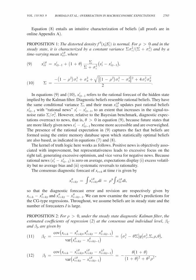
Equation (8) entails an intuitive characterization of beliefs (all proofs are in online Appendix A).
PROPOSITION 1: The distorted density f θ ( x t | S t i ) is normal. For ρ > 0 and in the steady state, it is characterized by a constant variance Σ σ ϵ 2 /(Σ + σ ϵ 2 ) and by a time-varying mean x t | t i,θ , where
(9) x t | t i,θ = x t | t−1 i + (1 + θ) Σ _ Σ + σ ϵ 2
( s t i − x t | t−1 i ) ,
(10) Σ = − (1 − ρ 2 ) σ ϵ 2 + σ u 2 + √
______________________ [ (1 − ρ 2 ) σ ϵ 2 − σ u 2 ] 2 + 4 σ ϵ 2 σ u 2 _______________________________________
2 .
In equations (9) and (10), x t | t−1 i refers to the rational forecast of the hidden state implied by the Kalman filter. Diagnostic beliefs resemble rational beliefs. They have the same conditional variance Σ , and their mean x t | t i,θ updates past rational beliefs x t | t−1 i with “rational news” s t i − x t | t−1 i , to an extent that increases in the signal-to-noise ratio Σ/ σ ϵ 2 . However, relative to the Bayesian benchmark, diagnostic expec-tations overreact to news, that is, θ > 0 in equation (9), because future states that are more likely given news s t i − x t | t−1 i become more accessible and are overweighed. The presence of the rational expectation in (9) captures the fact that beliefs are formed using the entire memory database upon which statistically optimal beliefs are also based, as indicated in equations (7) and (8).
The kernel of truth logic here works as follows. Positive news is objectively asso-ciated with improvement, but representativeness leads to excessive focus on the right tail, generating excessive optimism, and vice versa for negative news. Because rational news ( s t i − x t | t−1 i ) is zero on average, expectations display (i) excess volatil-ity but no average bias and (ii) systematic reversals to rationality.
The consensus diagnostic forecast of x t+h at time t is given by
x t+h | t θ = ∫ x t+h | t i,θ di = ρ h ∫
x t | t i,θ di ,
so that the diagnostic forecast error and revision are respectively given by x t+h − x t+h | t θ and x t+h | t θ − x t+h | t−1 θ . We can now examine the model’s predictions for the CG-type regressions. Throughout, we assume beliefs are in steady state and the number of forecasters I is large.
PROPOSITION 2: For ρ > 0 , under the steady state diagnostic Kalman filter, the estimated coefficients of regression (2) at the consensus and individual level, β C and β I , are given by
(11) β C = cov ( x t+h − x t+h | t θ , x t+h | t θ − x t+h | t−1 θ ) ________________________
var ( x t+h | t θ − x t+h | t−1 θ ) = ( σ ϵ 2 − θ Σ) g ( σ ϵ 2 , Σ, ρ, θ) ,
(12) β I = cov ( x t+h − x t+h | t i,θ , x t+h | t i,θ − x t+h | t−1 i,θ ) ________________________
var ( x t+h | t i,θ − x t+h | t−1 i,θ ) = −
θ (1 + θ) ____________
(1 + θ) 2 + θ 2 ρ 2 ,

2766 THE AMERICAN ECONOMIC REVIEW SEPTEMBER 2020
where g( σ ϵ 2 , Σ, ρ, θ ) > 0 is a function of parameters. Thus, for θ ∈ (0, σ ϵ 2 /Σ) the diagnostic Kalman filter entails a positive consensus coefficient β C > 0 and a neg-ative individual coefficient β I < 0 .
For θ > 0 , overreaction of individual forecasters to their own information rel-ative to the Bayesian benchmark implies negative predictability of forecast errors and thus a negative coefficient β I < 0 .17 At the same time, forecasters do not react at all to the information received by others (which they do not observe). This effect can create rigidity in the consensus forecast, provided representative types are not too overweighed relative to the dispersion of signals, θ < σ ϵ 2 /Σ . In this case, the diagnostic filter entails rigidity in consensus beliefs and a positive consensus coef-ficient. For such intermediate θ , the model thus reconciles the empirical patterns in Section II. Intuitively, even if each forecaster revises his own beliefs too much relative to what is prescribed by Bayes’ law, θ > 0 , if information is sufficiently noisy that each diagnostic agent discounts his own signal, then consensus forecasts exhibit rigidity.
Noisy rational expectations ( θ = 0 ) can generate the rigidity of consensus fore-casts, β C > 0 , but not overreaction of individual forecasters, β I < 0 . Because forecasters optimally use their information, their forecast error is uncorrelated with their own forecast revision. As is evident from equation (11), when θ = 0 there is no individual-level predictability, contrary to the evidence of Section II.
Finally, Proposition 2 also illustrates the cross-sectional implications of the kernel of truth: the predictability of forecast errors depends on the true parameters charac-terizing the data-generating process ( σ ϵ 2 , Σ, ρ, θ ) . In particular, stronger persistence ρ reduces individual overreaction, in the sense that it pushes the individual-level coefficient β I in equation (12) toward zero. Intuitively, rational forecast revisions for a very persistent series are large, which reduces the extent of revision variance that is due to overreaction and thus the predictability of errors. In Section IV we check this prediction in the data.
The qualitative properties of Proposition 2 continue to hold if forecasters have heterogeneous diagnostic distortions θ . Equation (12) characterizes the forecast error-on-revision regression coefficient for individual forecasters, as in Figure 1. With heterogeneity in θ , the estimated coefficients vary across forecasters (as observed in the data), so the pooled regression coefficient in equation (2) captures a weighted average of the forecaster-by-forecaster regression coefficients. As discussed in Section II, this coefficient can be biased upwards and is negative only if sufficiently many forecasters overreact. Finally, with heterogeneous θ s, the consensus coeffi-cients in equation (11) can be interpreted as depending on a suitably weighted aver-age of individual θ s. In this respect, the consensus coefficient is informative about an average bias in the population (see the proof of Proposition 2 for details).
We conclude this theoretical analysis by considering the possibility, relevant in many real-world settings, that forecasters also observe public signals. We focus on contemporaneous information (in Lemma A.1 we allow forecasters to observe
17 Overreaction here is driven by overweighting of representative types and is distinct from a mechanical depar-ture of the Bayesian balance between type I and type II errors (i.e., underreaction to fundamentals versus overreac-tion to noise), which would be akin to overconfidence.

2767BORDALO ET AL.: OVERREACTION IN MACROECONOMIC EXPECTATIONSVOL. 110 NO. 9
lagged hidden states). In financial markets, for instance, asset prices themselves sup-ply high-frequency, costless public signals that aggregate individual beliefs about future outcomes (though they also contain other shocks such as demand for liquid-ity). For macro variables as well, noisy public information can come from news releases. To see how public signals affect our analysis, suppose that each forecaster observes, in addition to the private signal s t i , a public signal s t = x t + v t , where v t is i.i.d. normal with variance σ v 2 . The diagnostic estimate now uses both the private and public signals according to their informativeness. We obtain the following result.
COROLLARY 1: Suppose that θ ∈ (0, σ ϵ 2 /Σ) . Then, increasing the precision 1/ σ v 2 of the public signal while holding constant the total precision (1/ σ ϵ 2 + 1/ σ v 2 ) of the private and public signals (i ) leaves the individual coefficient β I unchanged and (ii ) lowers the consensus coefficient β C .
When a higher share of information comes from a public signal, the information of different forecasters is more correlated, so individual forecasts incorporate more of the available information. The consensus forecast then exhibits less rigidity, or possibly even overreaction. This may explain why in financial variables such as interest rates we detect less consensus rigidity than in most other series: market prices act as public signals that correlate to a significant extent the information sets of different forecasters.
In this setting we can compare diagnostic expectations to overconfidence, typi-cally modeled as overweighting of private signals relative to public ones (Daniel, Hirshleifer, and Subrahmanyam 1998).18 By inflating the signal-to-noise ratio of private information, overconfidence creates overreaction to private signals and underreaction to public ones. As such, it cannot deliver the results of Corollary 1. More generally, under diagnostic expectations, the Kalman gain of both private and public information is multiplied by (1 + θ ) and so the reaction to information is not bounded by 1 (see equation (8)). A Kalman gain larger than one, which is equiva-lent to consensus-level overreaction, is needed to account for the evidence on con-sensus forecasts of federal government spending that we document here and for the evidence on consensus forecasts of the long-term earnings growth of individual firms documented in BGLS (2019). Our structural estimation exercise in online Appendix F finds additional evidence that Kalman gains above 1 help account for several series.
B. Back to the Data: Alternative Hypotheses and the Kernel of Truth
We can now go back to the estimates in Table 3. In our model, a positive θ is needed to explain the estimates for the 14 out of 22 series that display negative indi-vidual-level CG coefficients. This means that 12 out of the 18 economic variables we consider point to θ > 0 . These include key macro variables—such as nominal GDP, CPI, private consumption, industrial production, long-term interest rates—but also a predictor of systematic macro reversals, namely the BAA spread ( López-Salido,
18 Diagnostic expectations also describe beliefs where overconfidence can be ruled out (e.g., when all informa-tion is public, in experiments on base rate neglect or social stereotypes).

2768 THE AMERICAN ECONOMIC REVIEW SEPTEMBER 2020
Stein, and Zakrajšek 2017). Looking only at consensus forecasts for these variables would not uncover this finding. The evidence for 3 out of 18 variables, including the GDP deflator and investment series, is consistent with noisy information, namely θ = 0 in our setup. Finally, the data for the remaining 3 variables, unemployment and the short-term interest rates, exhibit underreaction at the individual level (we include unemployment here even though the median forecaster appears to overreact).
What can we make of these results? First, rational expectations are rejected by the data. Second, the majority of series point to overreaction θ > 0 , and consensus forecasts are always more rigid than individual ones, in line with the model. At the same time, there is a lot of variation in the extent of rigidity and overreaction in the data, and some patterns cannot be accounted for by diagnostic expectations, such as individual-level underreaction to news in short-term interest rates, which requires θ < 0 .
Before moving to the structural analysis, we assess whether broad patterns in the data are consistent with the kernel of truth property embedded in diagnostic expec-tations, particularly in comparison to the standard backward-looking model of adap-tive expectations. Several tests along these lines are reported in online Appendix E; here we offer a verbal synthesis.
Under diagnostic expectations, more persistent series should exhibit more cor-related revisions at different horizons. That is, for series that are more persistent, revisions for t + 2 should be more positively correlated with revisions for t + 3 . This prediction is strongly supported by the data (online Appendix E, Figure E1). Forecasters update in a forward-looking way in the sense that forecasts take the variable’s true persistence into account, even if they overreact to news. This finding is at odds with adaptive expectations, which specify that agents form expectations using a distributed lag of past realizations with fixed weights so that updating at any horizon is unrelated to the true features of the process. More generally, this finding is inconsistent with the idea that forecasters hold misspecified models that are not responsive to objective news, in line with the Lucas (1976) critique.
Another testable implication of the kernel of truth is that belief updating should also respond to other information that helps predict future outcomes. To examine this prediction, we depart from the assumption of AR(1) processes in equation (5). Specifically, suppose that a series follows an AR(2) process characterized by short-term momentum and long-term reversals,
(13) x t+3 = ρ 2 x t+2 + ρ 1 x t+1 + u t+3 ,
where ρ 2 > 0 and ρ 1 < 0 . In this case, which we examine in online Appendix E.2, diagnostic expectations entail an exaggeration of both short-term momentum and long-term reversals.
Formally, diagnostic expectations about the AR(2) process (13) yield two pre-dictions. First, as in the rational benchmark, an upward revision about t + 2 entails an upward revision about t + 3 , while an upward revision about t + 1 entails a downward revision about t + 3 . Second, and contrary to the rational benchmark, these revisions predict future errors due to overreaction. Thus, upward revisions about t + 2 lead to excess optimism about t + 3 (an exaggeration of short-term
2769BORDALO ET AL.: OVERREACTION IN MACROECONOMIC EXPECTATIONSVOL. 110 NO. 9
momentum), but upward revisions about t + 1 lead to excess pessimism about t + 3 (an exaggeration of reversal).
To test these predictions, we first assess which series are better described by AR(2) rather than by AR(1), so that ρ 1 is significantly negative and entails a better fit under the Bayesian information criterion (online Appendix E, Table E1). Consistent with Fuster, Laibson, and Mendel (2010), we find that several macroeconomic vari-ables exhibit hump-shaped dynamics with short-term momentum and longer-term reversals.19 We then show that the two predictions of diagnostic expectations hold in the data. First, for the vast majority of these series, the forecast error about t + 3 is negatively predicted by revisions about t + 2 but positively predicted by revisions about t + 1 . This behavior is consistent with the kernel of truth but not with more mechanical models, such as adaptive and natural expectations (Fuster, Laibson, and Mendel 2010) in which forecasters neglect long-term reversals. Second, and importantly, separating short-term persistence from long-term reversals clarifies the patterns of reaction to information. We now find evidence of overreaction even for unemployment and short-term rates, which displayed underreaction under the AR(1) specification.
In sum, the kernel of truth property holds predictive power. Diagnostic expec-tations capture forward-looking departures from rationality in a way that helps account for the data.
IV. Reaction to Information across Series
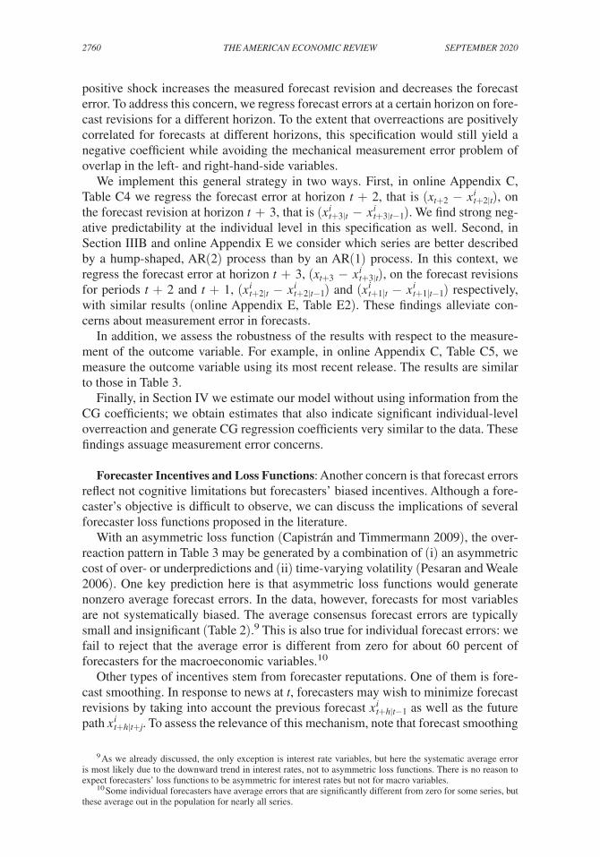
In this section, we assess the ability of our model to account for the different degrees of overreaction observed in individual forecasts of different economic series and for the relative rigidity of consensus forecasts. To see how the kernel of truth can shed light on these patterns, consider Proposition 2. Equation (12) predicts that the individual-level CG coefficients should depend on the persistence ρ of the economic variable and on the diagnosticity parameter θ . Similarly, equation (11) predicts that the consensus coefficients for a variable should depend on the same persistence parameter ρ , on diagnosticity θ , but also on the noise-to-signal ratio σ ϵ / σ u .
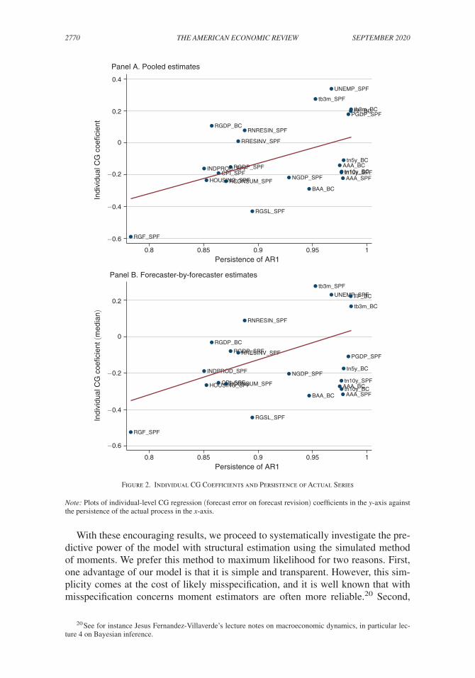
Because these predictions invoke nondirectly observable parameters such as diagnosticity θ and noise σ ϵ / σ u , in this section we recover the parameters from data using structural estimation techniques. First, however, we look at the raw data, which can be done for individual-level CG coefficients. Equation (12) offers in fact a straightforward prediction: for a given θ , these coefficients should be less negative for more persistent series. To test this prediction, we run an AR(1) specification of actuals for each series and estimate a series specific persistence parameter ρ . In Figure 2, panel A plots the correlation between the baseline pooled individual-level CG coefficients from Table 3 and ρ . Panel B displays the same plot but for median forecaster-by-forecaster CG coefficients from Table 3. Consistent with our model, the CG coefficient rises with persistence. For the pooled coefficient, the correlation is about 0.49 and statistically different from 0 with a p-value of 0.02. For the median individual-level coefficient, the correlation is 0.37 with p-value of 0.08.
19 We do not aim to find the unconstrained optimal ARMA(k, q) specification, which is notoriously difficult. We only wish to capture the simplest longer lags and see whether expectations react to them as predicted by the model.
2770 THE AMERICAN ECONOMIC REVIEW SEPTEMBER 2020
With these encouraging results, we proceed to systematically investigate the pre-dictive power of the model with structural estimation using the simulated method of moments. We prefer this method to maximum likelihood for two reasons. First, one advantage of our model is that it is simple and transparent. However, this sim-plicity comes at the cost of likely misspecification, and it is well known that with misspecification concerns moment estimators are often more reliable.20 Second,
20 See for instance Jesus Fernandez-Villaverde’s lecture notes on macroeconomic dynamics, in particular lec-ture 4 on Bayesian inference.
Figure 2. Individual CG Coefficients and Persistence of Actual Series
Note: Plots of individual-level CG regression (forecast error on forecast revision) coefficients in the y-axis against the persistence of the actual process in the x-axis.
NGDP_SPF
RGDP_SPF
RGDP_BC
CPI_SPFRCONSUM_SPF
INDPROD_SPF
RNRESIN_SPF
RRESINV_SPF
RGF_SPF
RGSL_SPF
HOUSING_SPF
UNEMP_SPF
FF_BC
tb3m_SPF
tn5y_BC
tn10y_SPFtn10y_BCAAA_SPF
AAA_BC
BAA_BC
−0.6
−0.4
−0.2
0
0.2
0.4
−0.6
−0.4
−0.2
0
0.2
Indi
vidu
al C
G c
oe�c
ient
0.8 0.85 0.9 0.95 1
Persistence of AR1
NGDP_SPF
RGDP_SPFRGDP_BC
PGDP_SPF
CPI_SPFRCONSUM_SPF
INDPROD_SPF
RNRESIN_SPF
RRESINV_SPF
RGF_SPF
RGSL_SPF
HOUSING_SPF
UNEMP_SPFFF_BCtb3m_SPF
tb3m_BC
tn5y_BC
tn10y_SPFtn10y_BCAAA_SPF
AAA_BCBAA_BC
Indi
vidu
al C
G c
oe�c
ient
(med
ian)
PGDP_SPFtb3m_BC
0.8 0.85 0.9 0.95 1
Persistence of AR1
Panel A. Pooled estimates
Panel B. Forecaster-by-forecaster estimates

2771BORDALO ET AL.: OVERREACTION IN MACROECONOMIC EXPECTATIONSVOL. 110 NO. 9
fundamental shocks can be fat tailed, and estimating a non-normal model by max-imum likelihood is problematic because the likelihood function cannot be written in closed form. Numerical approximations methods must be used, and these may introduce additional noise in parameter estimates.21 Our estimation exercise can be viewed as a useful first step in assessing the ability of our model to account for the variation in expectations errors.
We develop three estimation methods. In Method 1, we match series-specific parameters (θ, σ ε / σ u ) by fitting, for each series, the variance of forecast errors and forecast revisions. These are natural moments to target. First, they can be measured directly from the data. Second, they are linked to the parameters of interest. By the law of total variance, the variance of forecast errors σ FE,k 2 is the sum of (i) the average cross-sectional variance of errors and (ii) the variance over time of con-sensus errors. The first term is informative about the measurement noise σ ε,k , while the latter is informative about the overreaction parameter θ k . A similar logic holds for the total variance of forecast revisions. In a rational model with θ = 0 , large cross-sectional dispersion of forecasts is symptomatic of large noise σ ε,k , which would imply more cautious consensus revisions. A positive θ would instead help rec-oncile large cross-sectional dispersion in forecasts with large consensus revisions.22
Because this method does not use CG coefficients in the estimation, it allows us to assess how the model replicates both the consensus and individual regression results in Table 3. Positive estimates of θ help reconcile negative individual with positive consensus CG coefficients. Moreover, variation in θ across series tells us how much extra overreaction we need to fit the data, given our assumptions about the data-generating process and the signal structure.
In Methods 2 and 3 (Sections IVB and IVC), we estimate θ by directly fitting individual-level coefficients to the model prediction (equation (12)). This pins our estimates of θ more tightly to the model. We can then estimate the noise-to-signal ratio σ ϵ / σ u by fitting the variance of forecast revisions, which allows us to focus on variations for each forecaster over time (in comparison, the variance of forecast errors is more affected by fixed cross-sectional differences across individuals and as such is less reliable). Method 2 again allows θ to vary across series. Here, model performance is assessed by the ability to fit the consensus CG coefficient alone. Method 3 instead restricts θ to be the same for all series. This exercise allows for assessing the model’s explanatory power for the variation of both individual and consensus CG coefficients in terms of fundamental parameters ( ρ 1,k , σ u,k , σ ϵ,k ) .
All three estimation methods build on the following procedure. Each series k is described as an AR(1), using the fitted fundamental parameters ( ρ 1,k , σ u,k ) (online Appendix F, Table F1). Next, for each series x t k of actuals and parameter values ( θ k , σ ϵ,k ) , we simulate time series of signals s t i,k = x t k + ϵ t i,k , where ϵ t i,k is drawn from N(0, σ ϵ,k 2 ) i.i.d. across time and forecasters. We then use ( θ k , σ ϵ,k ) and s t i,k to
21 With the particle filter, numerically computing the marginal likelihood is challenging because the implied latent signals must be backed out from the observed forecast data. To do so, the particle filter must be applied for a grid of possible latent signals to match the observed forecast. This has to be applied at every observation for every individual and every series. Errors introduced in this procedure propagate to the estimate of implied signals over (panel) time.
22 In contrast, matching average forecast errors and revisions would not be informative about θ k and σ ε,k , as these sample moments are close to zero in our data (consistently with diagnostic but also rational expectations).

2772 THE AMERICAN ECONOMIC REVIEW SEPTEMBER 2020
generate diagnostic expectations, using equation (9). We generate diagnostic expec-tations for each forecaster in the sample, by using the realizations x t k over the exact period in which the forecaster makes predictions for series k (we drop forecasters with fewer than ten observations as before). We use these expectations to compute the relevant moments in each method and search through a parameter grid to mini-mize the relevant loss function as described below.
To assess how the model matches the empirical CG regression coefficients, model-predicted coefficients are computed as follows. For each series, the estimated ( θ , σ ϵ ) and the actual process parameters are used to generate model-based forecasts for each forecaster during the time period where the forecaster participates in the panel. We then run CG regressions using these model-based forecasts and compare the results with the empirical CG coefficients in Table 3.
In this estimation exercise, we abstract away from forecaster heterogeneity in θ . Although for many forecasters we may not have enough data to obtain precise esti-mates of their individual θ , online Appendix F performs a tentative analysis of the heterogeneous forecaster case following Method 2. We return to this in Section V.
A. Parameter Estimates
In Method 1, for each series k we search for the parameter values ( θ k , σ ε,k ) that best match the variance of the forecast errors, σ FE,k 2 = var i,t ( FE k,t i ) , and the vari-ance of forecast revisions, σ FR,k 2 = var i,t ( FR k,t i ) , computed across time and fore-casters. For values (θ, σ ϵ ) , denote the model-implied moments by σ ˆ FE,k 2 (θ, σ ϵ ) and σ ˆ FR,k 2 (θ, σ ϵ ) . We search through a grid of parameters for values that minimize the distance ( σ FE,k 2 − σ ˆ FE,k 2 (θ, σ ϵ )) 2 + ( σ FR,k 2 − σ ˆ FR,k 2 (θ, σ ϵ )) 2 . The grid imposes the model-based constraint θ ≥ 0 . Next, we evaluate the empirical covariance of the two moments at the first-stage parameters ( θ k,FS ∗ , σ ε,k,FS ∗ ) and invert it to obtain the optimal weight matrix W. Finally, we compute the second-stage estimate that mini-mizes the quadratic form,
( σ FE,k 2 − σ ˆ FE,k 2 (θ, σ ϵ ) , σ FR,k 2 − σ ˆ FR,k 2 (θ, σ ϵ ) ) T W ( σ FE,k 2 − σ ˆ FE,k 2 (θ, σ ϵ ) , σ FR,k 2 − σ ˆ FR,k 2 (θ, σ ϵ ) ) .
To obtain confidence intervals for our estimates, we bootstrap from the panel of forecasters with replacement.
In Method 2, we fit θ k by inverting the individual CG coefficient in equation (12) for each series k . We allow for negative values because we are interested in assessing the extent to which Methods 1 and 2 offer comparable results for the variation in θ across series. Using this fitted value of θ k , we then estimate σ ϵ,k by fitting the variance of forecast revisions, that is by minimizing the distance ( σ FR,k 2 − σ ˆ FR,k 2 (θ, σ ϵ ))
2 . In
Method 3 we estimate the model by restricting θ to be the same for all series. For each value θ , we estimate each series’ noise σ ϵ,k by matching the variance of fore-cast revisions and then calculate the individual CG coefficient for each variable. We find θ that minimizes the sum of mean-squared deviations between individual CG in the data and in the model (equal weighted across variables).
The estimation results for Methods 1 and 2 are summarized in Table 4. Here we describe the main results. In Method 1, we estimate significantly positive θ s for all series, ranging from 0.3 to 1.5 with an average of 0.59, and with tight confidence

2773BORDALO ET AL.: OVERREACTION IN MACROECONOMIC EXPECTATIONSVOL. 110 NO. 9
intervals.23 It might seem surprising that we find θ > 0 also for series such as unemployment and short-term interest rates for which the individual CG coefficients are positive, indicating underreaction. Recall, however, that in Method 1 we do not use these individual CG coefficients as inputs in the estimation. Positive θ in this estimation is consistent with cross-sectional heterogeneity in revisions coexisting with aggressive revisions in the consensus. In Method 2, by construction, the value of θ is positive for the 15 series that have negative individual CG regression coef-ficients and is negative for the remaining ones. The average θ is 0.42, which is close to the previous average estimate. The correlation between the values of θ in Methods 1 and 2 is 0.42 with p-value 0.00 (which increases to 0.88 if we exclude the RGF series, which is an outlier in Method 2), and the rank correlation is 0.87. Thus, the two methods yield comparable answers regarding the levels and variation in θ needed to make sense of the data.
Finally, under Method 3, the loss function reaches a tight minimum at θ = 0.5 , in line with the average values obtained with the other methods. In sum, model esti-mation strengthens the finding of overreaction. We report multiple sensitivity checks for this analysis in online Appendix F to confirm our main findings.24
23 For Method 1, both moments depend on both parameters, θ and σ ϵ , under the AR(1) assumption. Numerically, one can vary the parameters to test the sensitivity of the two moments. It turns out that the relative sensitivity of the two moments to the two parameters varies across the different series, so it is hard to draw a general lesson.
24 We highlight here three robustness tests. First, we allow series to be described as AR(2) processes and obtain similar results as here. This is reassuring given the well-known difficulty of finding the proper AR(k) specification. Second, we allow for fundamental shocks to be drawn from fat-tailed distributions, which requires implementing
Table 4—SMM Estimates of θ (Methods 1 and 2)
Method 1 Method 2
θ 95% CI θ 95% CI
Nominal GDP (SPF) 0.53 (0.42, 0.60) 0.29 (0.18, 0.43)Real GDP (SPF) 0.60 (0.56, 0.60) 0.18 (0.08, 0.31)Real GDP (BC) 0.34 (0.25, 0.42) −0.10 (−0.16, −0.03)GDP price index inflation (SPF) 0.55 (0.42, 0.60) −0.15 (−0.22, −0.08)CPI (SPF) 0.49 (0.35, 0.71) 0.25 (0.11, 0.40)Real consumption (SPF) 0.98 (0.80, 1.36) 0.34 (0.19, 0.53)Industrial production (SPF) 0.57 (0.44, 0.71) 0.20 (0.09, 0.35)Real nonresidential investment (SPF) 0.36 (0.25, 0.49) −0.07 (−0.14, 0.02)Real residential investment (SPF) 0.37 (0.25, 0.53) −0.01 (−0.11, 0.10)Real federal government consumption (SPF) 0.90 (0.62, 1.32) 5.46 (−3.38, 27.85)Real state and local government consumption (SPF) 1.37 (0.80, 2.31) 1.11 (0.74, 1.63)Housing start (SPF) 0.69 (0.53, 0.84) 0.32 (0.17, 0.53)Unemployment (SPF) 0.30 (0.30, 0.30) −0.28 (−0.35, −0.21)Fed funds rate (BC) 0.30 (0.30, 0.30) −0.17 (−0.21, −0.13)Three-month Treasury rate (SPF) 0.40 (0.35, 0.46) −0.23 (−0.27, −0.18)Three-month Treasury rate (BC) 0.30 (0.28, 0.30) −0.18 (−0.22, −0.14)Five-year Treasury rate (BC) 0.45 (0.39, 0.49) 0.13 (0.08, 0.18)Ten-year Treasury rate (SPF) 0.49 (0.41, 0.59) 0.25 (0.16, 0.34)Ten-year Treasury rate (BC) 0.49 (0.41, 0.53) 0.23 (0.15, 0.30)AAA corporate bond rate (SPF) 0.70 (0.56, 0.82) 0.32 (0.21, 0.45)AAA corporate bond rate (BC) 0.93 (0.79, 1.06) 0.17 (0.11, 0.24)BAA corporate bond rate (BC) 0.70 (0.53, 0.79) 0.47 (0.33, 0.63)
Notes: This table shows the estimates of θ and the 95 percent confidence interval using 300 bootstrap samples (bootstrapping forecasters with replacement). Results for each series are estimated using the AR(1) version of the diagnostic expectations model based on the properties of the actuals according to online Appendix F Table F1. In Method 2, we first estimate θ using the individual CG regression coefficient in the data (pooled estimates as in Table 3) and the formula in equation (12).

2774 THE AMERICAN ECONOMIC REVIEW SEPTEMBER 2020
The estimates for θ are on average somewhat smaller but in line with BGS (2018), who obtain θ = 0.9 for expectations data on credit spreads, and with BGLS (2019) who also obtain θ = 0.9 for expectations data on firm-level earnings’ growth. To give a sense of the magnitude, a θ ≈ 0.5 means that forecasters’ reaction to news is roughly 50 percent larger than the rational expectations benchmark. This fact alone suggests that the resulting distortions in beliefs can have sizable economic consequences. In fact, BGLS (2019) find that θ = 0.9 can account for the observed 12 percent annual return spread between stocks that long-term earnings growth ana-lysts are pessimistic about and stocks they are optimistic about. Bordalo, Gennaioli, Shleifer, and Terry (2019) find that an RBC model with a θ in the range of 0.5–1 gen-erates large boom-bust cycles in credit spreads, leverage, and aggregate investment. We return to the implications of belief distortions of this magnitude in Section V.
Finally, we turn to the estimates of noise σ ϵ , which we normalize by the standard deviation of shocks σ u . Tables F2 and F8 in online Appendix F report the results. Consistent with rigidity of consensus forecasts, individual noise is larger than fun-damental innovations, with the average estimated σ ϵ / σ u ranging from 1.30 to 1.74 across methods. In the next section we assess the model’s performance by exam-ining whether our estimates of parameters θ and σ ϵ can account for differences in individual and consensus CG coefficients across series.
B. Model Performance
To assess the performance of the model, we examine how the model matches the empirical CG regression coefficients.25 As discussed above, for each series use the estimated ( θ , σ ϵ ) to generate model-based CG regressions at the individual and con-sensus levels and compare the results with the empirical CG coefficients in Table 3. Figure 3 plots the individual CG coefficients (left column) and the consensus coef-ficients (right column) from each of the estimated models against those from the survey data.
In Method 1, for individual CG coefficients, the correlation between the empir-ical estimates and the model predictions is high, about 0.76 ( p-value of 0.00). In levels, the individual CG coefficients implied by the model tend to be more positive than those in the data. Even so, given its parsimony, the model does an impressive job capturing cross-sectional differences. For consensus CG coefficients, we also find a positive correlation of 0.18 ( p-value of 0.44) between the model and the data. This lower correlation likely reflects, at least in part, the fact that consensus coeffi-cients are highly dependent on the magnitude of measurement noise σ ϵ,k , which is in turn estimated with some imprecision.
We next examine Method 2. By construction, the method accounts well for indi-vidual-level CG coefficients, with a correlation between coefficients in the model
the numerical particle filter method. Again, our results remain stable. Finally, we perform the analysis at the level of individual forecasters and again obtain similar results for the median forecaster.
25 In online Appendix F, we show that the model offers a satisfactory fit of the target moments across series under each method. In Method 1, the average absolute log difference between the variance of forecast errors in the data ( σ FE,k 2 ) and in the simulated model ( σ ˆ FE,k 2 (θ, σ ϵ ) ) is 0.05, and that for the variance of forecast revision is 0.06 (Table F3). For Method 2 and Method 3, the variance of forecast revision is the only target moment, and the average absolute log difference between the data and model moments is 0.56 and 0.09 respectively (Tables F9 and F12).
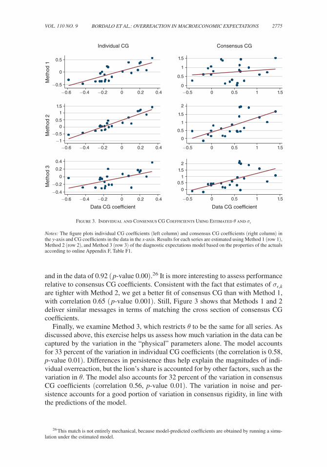
2775BORDALO ET AL.: OVERREACTION IN MACROECONOMIC EXPECTATIONSVOL. 110 NO. 9
and in the data of 0.92 ( p-value 0.00).26 It is more interesting to assess performance relative to consensus CG coefficients. Consistent with the fact that estimates of σ ϵ,k are tighter with Method 2, we get a better fit of consensus CG than with Method 1, with correlation 0.65 ( p-value 0.001). Still, Figure 3 shows that Methods 1 and 2 deliver similar messages in terms of matching the cross section of consensus CG coefficients.
Finally, we examine Method 3, which restricts θ to be the same for all series. As discussed above, this exercise helps us assess how much variation in the data can be captured by the variation in the “physical” parameters alone. The model accounts for 33 percent of the variation in individual CG coefficients (the correlation is 0.58, p-value 0.01). Differences in persistence thus help explain the magnitudes of indi-vidual overreaction, but the lion’s share is accounted for by other factors, such as the variation in θ . The model also accounts for 32 percent of the variation in consensus CG coefficients (correlation 0.56, p-value 0.01). The variation in noise and per-sistence accounts for a good portion of variation in consensus rigidity, in line with the predictions of the model.
26 This match is not entirely mechanical, because model-predicted coefficients are obtained by running a simu-lation under the estimated model.
Figure 3. Individual and Consensus CG Coefficients Using Estimated θ and σ ϵ
Notes: The figure plots individual CG coefficients (left column) and consensus CG coefficients (right column) in the y-axis and CG coefficients in the data in the x-axis. Results for each series are estimated using Method 1 (row 1), Method 2 (row 2), and Method 3 (row 3) of the diagnostic expectations model based on the properties of the actuals according to online Appendix F, Table F1.
−0.5
0
0.5
Met
hod
1
−0.6 −0.4 −0.2 0 0.2 0.4
−0.6 −0.4 −0.2 0 0.2 0.4
−0.6 −0.4 −0.2 0 0.2 0.4
Individual CG
0
0.5
1
1.5
−0.5 0 0.5 1 1.5
−0.5 0 0.5 1 1.5
Consensus CG
−1
−0.5
00.5
11.5
Met
hod
2
0
0.5
1
1.5
2
0
0.51
1.52
−0.5 0 0.5 1 1.5
−0.4
−0.2
0
0.2
0.4
Met
hod
3
Data CG coefficient Data CG coefficient

2776 THE AMERICAN ECONOMIC REVIEW SEPTEMBER 2020
Overall, the three estimation methods provide a robust and coherent picture that (i) individual overreaction is prevalent, (ii) the model captures variation in both individual and consensus CG coefficients as a function of fundamental parameters, and (iii) allowing θ to vary across series improves model performance. In online Appendix F, we examine several variations on these specifications, including allow-ing the series to be described as AR(2) processes, considering median individu-al-level forecasts, and allowing for non-normal shocks. The results are very similar.
V. Taking Stock
We summarize and interpret our main findings, discuss some open issues, and conclude.
A. Determinants of CG Coefficients
We consider the extent to which differences across economic variables in per-sistence ρ , noise-to-signal ratio σ ϵ / σ u , diagnosticity parameter θ , and the availability of public signals (Corollary 1) can explain the variation in CG coefficients.
Persistence ρ .—Figure 2 shows that, as predicted by the model, individual CG coefficients are more negative for less persistent series. Less persistent series such as government consumption, private consumption, or housing starts display clear over-reaction, while very persistent series such as unemployment or short-term interest rates display less overreaction or even underreaction at the individual level. Model estimates with Method 3, in which θ is kept constant, indicate that persistence alone accounts for 33 percent of the cross-sectional variation in individual CG coeffi-cients. Since allowing θ to vary accounts for roughly 57 percent of such variation with Method 1, and 85 percent in Method 2, differences in persistence account for between 39 percent and 58 percent of the model’s explanatory power in this dimension.27
Noise σ ϵ / σ u .—Noise in individual signals reconciles individual-level overreac-tion with consensus rigidity. Noisier information means that individual forecasts neglect a larger share of the average signal, making the consensus more rigid. Dispersed information and individual noise appear to play a significant role in the data, both because the dispersion of forecasts is large and because at the consensus level the prevalent pattern is informational rigidity.28
Using Method 3, allowing variation only in persistence and noise-to-signal ratio, our model accounts for 32 percent of variation in consensus CG coefficients. As one allows θ to vary in Method 2, the explained variation rises to 42 percent. In particu-lar, variation in the “physical” parameters ρ and σ ϵ / σ u accounts for two-thirds of the model’s explanatory power with respect to consensus CG coefficients.
27 It is harder to quantify the role of persistence for the consensus forecasts because in equation (11) the consen-sus CG coefficient is a highly nonlinear, nonmonotonic function of ρ .
28 The exception is federal government consumption, which displays statistically significant overreaction at the consensus level. This series is characterized by low persistence and low noise, as predicted by the model.

2777BORDALO ET AL.: OVERREACTION IN MACROECONOMIC EXPECTATIONSVOL. 110 NO. 9
Diagnosticity θ .—The average level of θ in any estimation method is close to 0.5, the tightly identified point estimate when θ is constrained to be the same across series (Method 3). With Methods 1 and 2, θ displays some variation, which helps account for the data. Variation in θ is more important for capturing individual than consensus CG coefficients, consistent with the model. What may this variation in θ capture? On the one hand, θ may capture specific factors that are outside the simple specification used in the estimation. On the other hand, variation in θ may corre-spond to actual variation in the tendency to overreact to news. We briefly comment on both mechanisms.
Variation in θ may in principle capture misspecification of the data-generat-ing process for actuals. We explore this possibility using the AR(2) specification of online Appendix E. Individual CG coefficients are no longer given by equa-tion (12), so we estimate the model under Method 1. Allowing for AR(2) dynam-ics does not sensibly alter our structural estimates, indicating that our ability to account for the cross section is robust to misspecification. Recall that empirically, as described in Section IIIB, this specification generates diagnostic overreaction in both unemployment and short-term interest rates, but it does not reduce varia-tion in estimated θ .
Variation in θ may also proxy for features of the information structure that may shape overreaction, particularly at the consensus level, such as public signals. In particular, the fact that θ is higher for financial series than for macroeconomic ones is consistent with the observation that the latter display more consensus rigidity. Also consistent with this view, in financial markets asset prices act as public sig-nals to which all agents can simultaneously overreact, as in Corollary 1. In goods markets, information is likely more dispersed, increasing consensus rigidity. In this respect, incorporating noisy public signals may help improve the explanatory power of the model.
On the other hand, the results may capture real variation in the tendency to over-react to information, driven perhaps by the extent to which judgments rely on intu-ition versus models and deliberation. Consistent with this hypothesis, individual forecasters’ estimated θ s are correlated across series. Within-forecaster variation in θ , in the cross section of series, may in turn depend on the decision-maker’s incentives and effort. Forecasts of key indicators such as GDP, unemployment, or inflation may have lower estimated θ s because forecasters spend more effort on them, producing forecasts that make better use of the available information. We leave a systematic assessment of this hypothesis to future work.
B. Open Issues
Our results contribute to the growing literature on nonrational expectations and help account for some potentially conflicting evidence, especially on consensus ver-sus individual expectations. Yet many issues remain open. Here we discuss three: evidence for overreaction in consensus forecasts, evidence for underreaction in indi-vidual forecasts, and the mapping between expectations and market outcomes.
Our model reconciles the evidence of rigidity of consensus forecasts, as doc-umented by CG (2015) and Table 3, with individual forecasters’ overreaction to news. Importantly, it can also reconcile the apparent rigidity of consensus forecasts

2778 THE AMERICAN ECONOMIC REVIEW SEPTEMBER 2020
for some variables with their overreaction for others, such as government spend-ing. As we already discussed, consensus overreaction has also been found in other data, such as BGLS (2019) finding strong overreaction of consensus forecasts of long-term ( 3–5 years) corporate earnings growth of listed firms in the United States. In our model, if news are dispersed ( σ ϵ is large), then aggregating beliefs entails consensus rigidity. If in contrast fundamental volatility σ u is high relative to dis-persed information, or if there are public signals that aggregate news (e.g., in finan-cial series), then the consensus forecast is more likely to overreact. The properties of consensus forecasts reflect the balance between these two forces and vary in predictable ways across variables. Consensus overreaction is itself a distinctive sign of diagnostic expectations.
But the central prediction of our model is overreaction at the level of individual forecasters. This is largely confirmed in our data (Table 3) and also in recent experi-mental research (Landier, Ma, and Thesmar 2019). However, we also find individual underreaction for short-term interest rates in Table 3. In earlier work, Bouchaud et al. (2019) document predominant individual-level underreaction in short-term (12 months ahead) earnings forecasts for US listed firms. We do not yet have a way to unify under- and overreaction at the individual level, but the evidence suggests that the term structure of expectations may play a role. In our Tables 3 and 4, indi-vidual underreaction prevails with respect to short-term interest rates, while over-reaction prevails with respect to long-term interest rates. The same pattern arises in the case of earnings forecasts: in Bouchaud et al. (2019), individual underreaction occurs for short-term forecasts, while in BGLS (2019) overreaction occurs for long-term forecasts.
Is this term structure consistent with diagnostic expectations? Preliminary anal-ysis suggests that the answer may be yes. In the case of interest rates, we showed that the greater overreaction of forecasts for long-term outcomes is consistent with the kernel of truth logic. Long-term interest rates are less persistent than short-term ones, which implies that overreaction should be stronger for the former, consistent with the evidence. A similar mechanism may be at play with respect to short- ver-sus long-term corporate earnings. Furthermore, D’Arienzo (2019) shows in the context of interest rates that another mechanism is at play: long-term outcomes display a higher fundamental uncertainty σ u than short-term outcomes. Beliefs may overreact more aggressively for long-term outcomes because it is easier to entertain the possibility of more extreme outcomes (since news reduces uncertainty less for outcomes in the far future). This mechanism is not in our current model, but, as D’Arienzo (2019) shows, it follows naturally from the logic of diagnostic expectations. Using this mechanism, he is able to account for a large chunk of the excess volatility of long-term rates relative to short-term ones documented by Giglio and Kelly (2018). In sum, although we do not have full unification and a force for individual underreaction may need to be added, the kernel of truth logic presents a promising mechanism for unifying departures from rational expectations.
Finally, consider the evidence of rigidity versus overreaction of beliefs in the con-text of market outcomes. In macroeconomics, several papers stress the importance of consensus rigidity to account for the apparent slow response to shocks of macro aggregates such as consumption and inflation (e.g., Sims 2003, Mankiw and Reis 2002). Other work, predominantly in finance, invokes overreaction to information

2779BORDALO ET AL.: OVERREACTION IN MACROECONOMIC EXPECTATIONSVOL. 110 NO. 9
to account for excess volatility in stock prices (Shiller 1981, BGLS 2019) and long-term interest rates (Giglio and Kelly 2018, D’Arienzo 2019) and for predictable reversals in stock returns (De Bondt and Thaler 1985, BGLS 2019). Part of the dif-ferences in these market outcomes may be accounted for by the comparative statics stressed in our analysis. For instance, financial assets may exhibit stronger overreac-tion because their valuations depend on distant future cash flows, which display low persistence, and because prices serve as public signals. In contrast, key macroeco-nomic outcomes may display more consensus rigidity because they depend on more persistent factors and because public signals are weaker.
The response of market outcomes to news also depends on the market process that translates beliefs into prices and quantities. Properties of consensus forecasts need not be the same as properties of aggregate outcomes. For instance, if individuals can leverage and returns are not strongly diminishing, then individual forecasts matter more for market outcomes (Buraschi, Piatti, and Whelan 2018). This may contrib-ute to overreaction in financial markets. In contrast, if market outcomes depend more symmetrically on many individual choices, for example in determining aggre-gate inflation, then the consensus forecast and its rigidity may be a better guide to expectations shaping market outcomes. Yet even in this case, with sustained news all individuals may react in the same direction leading to aggregate overreaction. This consideration opens intriguing directions to assess the relevance of overreac-tion or rigidity of beliefs in macroeconomic models starting from micro-founded belief updating.
C. Conclusion
Using data from Blue Chip and SPF, we study how professional forecasters react to news, building on the methodology of CG (2015). We find that while information rigidity prevails for the consensus forecast, as previously shown by CG (2015), for individual forecasters the prevalent pattern is overreaction, in the sense of upward forecast revisions generating forecasts that are too high relative to actual realiza-tions. These results are robust to many possible confounds. We then apply a psycho-logically founded model of belief formation, diagnostic expectations, to this data, and show that it can reconcile these seemingly contradictory patterns but also make several new predictions for the patterns of expectation errors across different series. The extent of individual overreaction, captured by the diagnostic parameter, is siz-able. According to our estimates in this and other papers, the rational response to news is inflated by a factor between 0.5 and 1. We view this as a starting estimate for macroeconomic quantification exercises, such as Bordalo, Gennaioli, Shleifer, and Terry (2019).
For the purpose of applied analysis then, the question becomes, what are the macroeconomic consequences of diagnostic expectations? At first glance, one might think that what matters for aggregate outcomes is consensus expectations, so rigid-ity is enough. This view misses two key points.
First, macroeconomics has advanced over the last several decades by starting with micro parameters estimated from micro data. The micro parameter θ estimated here and in related work lies between 0.5 and 1 and points to substantial overreaction by individual forecasters. As with other parameters, macroeconomic models grounded

2780 THE AMERICAN ECONOMIC REVIEW SEPTEMBER 2020
in micro estimates should then start with overreaction in expectations. This may be especially important for heterogeneous agent models with nonlinearities and lever-age, which stress the relevance of the micro units as opposed to the representative agent.
Second, there are reasons to doubt that consensus beliefs are always character-ized by rigidity. First, for some important long-term outcomes the consensus may overreact. This has been documented for long-term earnings (BGLS 2019) and may be generally true for beliefs and hence prices of distant cash flows (Giglio and Kelly 2018, D’Arienzo 2019). Such long-term movements may be key for asset prices and investment. Second, if information diffuses slowly, the reaction to a shock may see a gradual buildup of individual overreactions, taking some time to show as overreac-tion in the consensus forecasts or in aggregate outcomes.29 Analogously to short-run momentum and long-run reversals in the stock market, there can be investment cycles with slow accumulation of capital but ultimate excess capacity. More work is needed to assess whether such “delayed overreaction” can be detected in the data. Third, and critically, at certain junctures news may be correlated across agents, for instance if major innovations are introduced or if repeated news in the same direc-tion provides highly informative evidence of large changes. In these cases, which resemble our analysis of public signals, aggregate overreaction is likely to prevail.
Evidence symptomatic of aggregate overreaction has appeared in research on credit cycles. Buoyant credit markets and extreme optimism about firms’ perfor-mance predict slowdowns in investment and GDP growth, disappointing realized bond returns, and disappointing returns in bank stocks (Greenwood and Hanson 2013; López-Salido, Stein, and Zakrajšek 2017; Gulen, Ion, and Rossi 2018; Baron and Xiong 2017). Whether diagnostic expectations can offer a coherent and micro-founded theory for these and other macroeconomic phenomena is an import-ant question for future work.
REFERENCES
Adam, Klaus, Albert Marcet, and Johannes Beutel. 2017. “Stock Price Booms and Expected Capital Gains.” American Economic Review 107 (8): 2352–2408.
Amromin, Gene, and Steven A. Sharpe. 2014. “From the Horse’s Mouth: Economic Conditions and Investor Expectations of Risk and Return.” Management Science 60 (4): 4: 845–66.
Augenblick, Ned, and Eben Lazarus. 2018. “Restrictions on Asset-Price Movements under Rational Expectations: Theory and Evidence.” Unpublished.
Bacchetta, Philippe, Elmar Mertens, and Eric van Wincoop. 2009. “Predictability in Financial Mar-kets: What Do Survey Expectations Tell Us?” Journal of International Money and Finance 28 (3): 406–26.
Baron, Matthew, and Wei Xiong. 2017. “Credit Expansion and Neglected Crash Risk.” Quarterly Jour-nal of Economics 132 (2): 713–64.
Ben-David, Itzhak, John R. Graham, and Campbell R. Harvey. 2013. “Managerial Miscalibration.” Quarterly Journal of Economics 128 (4): 1547–84.
Benigno, Pierpaolo, and Anastasios G. Karantounias. 2019. “Overconfidence, Subjective Perception and Pricing Behavior.” Journal of Economic Behavior and Organization 164: 107–32.
Berger, Helge, Michael Ehrmann, and Marcel Fratzscher. 2011. “Geography, Skills or Both: What Explains Fed Watchers’ Forecast Accuracy of US Monetary Policy?” Journal of Macroeconom-ics 33 (3): 420–37.
29 We have formally proved this point by introducing diagnostic expectations into a Mankiw and Reis (2003) model of information rigidities. The results are available upon request.

2781BORDALO ET AL.: OVERREACTION IN MACROECONOMIC EXPECTATIONSVOL. 110 NO. 9
Beshears, John, James J. Choi, Andreas Fuster, David Laibson, and Brigitte C. Madrian. 2013. “What Goes Up Must Come Down? Experimental Evidence on Intuitive Forecasting.” American Eco-nomic Review 103 (3): 570–74.
Blue Chip Publications. 1983–2016. “Blue Chip Financial Forecasts.” https://lrus.wolterskluwer.com/store/blue-chip-publications/ (accessed February 28, 2017).
Bordalo, Pedro, Katherine Coffman, Nicola Gennaioli, and Andrei Shleifer. 2016. “Stereotypes.” Quar-terly Journal of Economics 131 (4): 1753–94.
Bordalo, Pedro, Nicola Gennaioli, Rafael La Porta, and Andrei Shleifer. 2019. “Diagnostic Expecta-tions and Stock Returns.” Journal of Finance 74 (6): 2839–74.
Bordalo, Pedro, Nicola Gennaioli, Yueran Ma, and Andrei Shleifer. 2020. “Replication Data for: Overreaction in Macroeconomic Expectations.” American Economic Association [publisher], Inter-university Consortium for Political and Social Research [distributor]. https://doi.org/10.3886/E118422V1.
Bordalo, Pedro, Nicola Gennaioli, and Andrei Shleifer. 2018. “Diagnostic Expectations and Credit Cycles.” Journal of Finance 73 (1): 199–227.
Bordalo, Pedro, Nicola Gennaioli, Andrei Shleifer, and Stephen J. Terry. 2019. “Real Credit Cycles.” Unpublished.
Bouchaud, Jean-Philippe, Philipp Krüger, Augustin Landier, and David Thesmar. 2019. “Sticky Expectations and the Profitability Anomaly.” Journal of Finance 74 (2): 639–74.
Broer, Tobias, and Alexandre Kohlhas. 2018. “Forecaster (Mis)-Behavior.” Unpublished.Buraschi, Andrea, Ilaria Piatti, and Paul Whelan. 2018. “Rationality and Subjective Bond Risk Pre-
mia.” Unpublished.Capistrán, Carlos, and Allan Timmermannn. 2009. “Disagreement and Biases in Inflation Expecta-
tions.” Journal of Money, Credit and Banking 41 (2–3): 365–96.Carroll, Christopher D. 2003. “Macroeconomic Expectations of Households and Professional Fore-
casters.” Quarterly Journal of Economics 118 (1): 269–98.Cieslak, Anna. 2018. “Short-Rate Expectations and Unexpected Returns in Treasury Bonds.” Review
of Financial Studies 31 (9): 3265–3306.Coibion, Olivier, and Yuriy Gorodnichenko. 2012. “What Can Survey Forecasts Tell Us about Infor-
mation Rigidities?” Journal of Political Economy 120 (1): 116–59.Coibion, Olivier, and Yuriy Gorodnichenko. 2015. “Information Rigidity and the Expectations Forma-
tion Process: A Simple Framework and New Facts.” American Economic Review 105 (8): 2644–78.Daniel, Kent, David Hirshleifer, and Avanidhar Subrahmanyam. 1998. “Investor Psychology and
Security Market Under- and Overreactions.” Journal of Finance 53 (6): 1839–85.D’Arienzo, Daniele. 2019. “Excess Volatility with Increasing Over-Reaction.” Unpublished.De Bondt, Werner F. M., and Richard H. Thaler. 1985 “Does the Stock Market Overreact?” Journal
of Finance 40 (3): 793-805Doucet, Arnaud, Nando de Freitas, and Neil Gordon, eds. 2001. Sequential Monte Carlo Methods in
Practice. New York: Springer.Frydman, Cary, and Gideon Nave. 2016. “Extrapolative Beliefs in Perceptual and Economic Deci-
sions: Evidence of a Common Mechanism.” Management Science 63 (7): 2340–52.Fuhrer, Jeffrey C. 2019. “Intrinsic Expectations Persistence: Evidence from Professional and House-
hold Survey Expectations.” Unpublished.Fuster, Andreas, David Laibson, and Brock Mendel. 2010. “Natural Expectations and Macroeconomic
Fluctuations.” Journal of Economic Perspectives 24 (4): 67–84.Gabaix, Xavier. 2014. “A Sparsity-Based Model of Bounded Rationality.” Quarterly Journal of Eco-
nomics 129 (4): 1661–1710.Gennaioli, Nicola, Yueran Ma, and Andrei Shleifer. 2016. “Expectations and Investment.” In NBER
Macroeconomics Annual 2015, Vol. 30, edited by Martin Eichenbaum and Jonathan A. Parker, 379–431. Chicago: University of Chicago Press.
Gennaioli, Nicola, and Andrei Shleifer. 2010. “What Comes to Mind.” Quarterly Journal of Economic 125 (4): 1399–1433.
Giglio, Stefano, and Bryan Kelly. 2018. “Excess Volatility: Beyond Discount Rates.” Quarterly Jour-nal of Economics 133 (1): 71–127.
Greenwood, Robin, and Samuel G. Hanson. 2013. “Issuer Quality and Corporate Bond Returns.” Review of Financial Studies 26 (6): 1483–1525.
Greenwood, Robin, and Andrei Shleifer. 2014. “Expectations of Returns and Expected Returns.” Review of Financial Studies 27 (3): 714–46.
Gulen, Huseyin, Mihai Ion, and Stefano Rossi. 2018. “Credit Cycles and Corporate Investment.” Unpublished.

2782 THE AMERICAN ECONOMIC REVIEW SEPTEMBER 2020
Hansen, Lars Peter, and Thomas J. Sargent. 2008. Robustness. Princeton, NJ: Princeton University Press.
Hjalmarsson, Erik. 2008. “The Stambaugh Bias in Panel Predictive Regressions.” Finance Research Letters 5 (1): 47–58.
Hommes, Cars, Joep Sonnemans, Jan Tuinstra, and Henk van de Velden. 2004. “Coordination of Expectations in Asset Pricing Experiments.” Review of Financial Studies 18 (3): 955–80.
Kahneman, Daniel, and Amos Tversky. 1972. “Subjective Probability: A Judgment of Representative-ness.” Cognitive Psychology 3 (3): 430–54.
Kendall, M. G. 1954. “Note on Bias in the Estimation of Autocorrelation.” Biometrika 41 (3): 403–04.Kohlhas, Alexandre, and Ansgar Walther. 2018. “Asymmetric Attention.” Unpublished.Landier, Augustin, Yueran Ma, and David Thesmar. 2019. “New Experimental Evidence on Expecta-
tions Formation.” Unpublished.La Porta, Rafael. 1996. “Expectations and the Cross-Section of Stock Returns.” Journal of Finance
51 (5): 1715–42.Liu, Jun S., and Rong Chen. 1998. “Sequential Monte Carlo Methods for Dynamic Systems.” Journal
of the American Statistical Association 93 (443): 1032–44.López-Salido, David, Jeremy C. Stein, and Egon Zakrajšek. 2017. “Credit-Market Sentiment and the
Business Cycle.” Quarterly Journal of Economics 132 (3): 1373–1426.Lucas, Robert E. 1976. “Econometric Policy Evaluation: A Critique.” Carnegie-Rochester Conference
Series on Public Policy 1: 19–46.Mankiw, N. Gregory, and Ricardo Reis. 2002. “Sticky Information versus Sticky Prices: A Proposal to
Replace the New Keynesian Phillips Curve.” Quarterly Journal of Economics 117 (4): 1295–1328.Moore, Don A., and Paul J. Healy. 2008. “The Trouble with Overconfidence.” Psychological Review
115 (2): 502–17.Morris, Stephen, and Hyun Song Shin. 2002. “Social Value of Public Information.” American Eco-
nomic Review 92 (5): 1521–34.Newey, Whitney K., and Kenneth D. West. 1994. “Automatic Lag Selection in Covariance Matrix Esti-
mation.” Review of Economic Studies 61 (4): 631–53.Nickell, Stephen. 1981. “Biases in Dynamic Models with Fixed Effects.” Econometrica 49 (6): 1417–
26.Orlik, Anna, and Laura Veldkamp. 2015. “Understanding Uncertainty Shocks and the Role of Black
Swans.” Unpublished.Ottaviani, Marco, and Peter Sørensen. 2006. “The Strategy of Professional Forecasting.” Journal of
Financial Economics 81 (2): 441–66. Pesaran, M. Hashem, and Martin Weale. 2006. “Survey Expectations.” In Handbook of Economic
Forecasting, Vol. 1, edited by G. Elliott, C. W. J. Granger, and A. Timmermannn, 715–76. Amster-dam: North-Holland.
Real-Time Data Set for Macroeconomists. 1968–2016. “Historical Data Files for the Real-Time Data Set for Macroeconomists.” Federal Reserve Bank of Philadelphia. https://www.philadelphiafed.org/research-and-data/real-time-center/real-time-data/data-files (accessed January 12, 2019).
Shiller, Robert J. 1981. “Do Stock Prices Move Too Much to Be Justified by Subsequent Changes in Dividends?” American Economic Review 71 (3): 421–36.
Sims, Christopher A. 2003. “Implications of Rational Inattention.” Journal of Monetary Economics 50 (3): 665–90.
Stambaugh, Robert F. 1999. “Predictive Regressions.” Journal of Financial Economics 54 (3): 375–421.
Survey of Professional Forecasters. 1968–2016. “Historical Data Files for the Survey of Professional Forecasters.” Federal Reserve Bank of Philadelphia. https://www.philadelphiafed.org/research-and-data/real-time-center/survey-of-professional-forecasters (accessed January 12, 2019).
Woodford, Michael. 2003. “Imperfect Common Knowledge and the Effects of Monetary Policy.” In Knowledge, Information, and Expectations in Modern Macroeconomics: In Honor of Edmund S. Phelps, edited by Philippe Aghion et al., 25–58. Princeton, NJ: Princeton University Press.