Output-Sensitive Autocompletion Search

Output-Sensitive Autocompletion Search

Holger Bast1, Christian W. Mortensen2, and Ingmar Weber1

1 Max-Planck-Institut fur Informatik, Saarbrucken, Germany{bast, iweber}@mpi-inf.mpg.de2 IT University of Copenhagen, Denmark

[email protected]

Abstract. We consider the following autocompletion search scenario: imagine auser of a search engine typing a query; then with every keystroke display thosecompletions of the last query word that would lead to the best hits, and alsodisplay the best such hits. The following problem is at the core of this feature:for a fixed document collection, given a set D of documents, and an alphabeticalrange W of words, compute the set of all word-in-document pairs (w, d) from thecollection such that w ∈ W and d ∈ D. We present a new data structure with thehelp of which such autocompletion queries can be processed, on the average, intime linear in the input plus output size, independent of the size of the underlyingdocument collection. At the same time, our data structure uses no more spacethan an inverted index. Actual query processing times on a large test collectioncorrelate almost perfectly with our theoretical bound.

1 Introduction

Autocompletion, in its most basic form, is the following mechanism: the user types thefirst few letters of some word, and either by pressing a dedicated key or automaticallyafter each key stroke a procedure is invoked that displays all relevant words that arecontinuations of the typed sequence. The most prominent example of this feature is thetab-completion mechanism in a Unix shell. In the recently launched Google Suggestservice frequent queries are completed. Algorithmically, this basic form of autocom-pletion merely requires two simple string searches to find the endpoints of the range ofcorresponding words.

1.1 Problem Definition

The problem we consider in this paper is derived from a more sophisticated form of au-tocompletion, which takes into account the context in which the to-be-completed wordhas been typed. Here, we would like an (instant) display of only those completionsof the last query word which lead to hits, as well as a display of such hits. For ex-ample, if the user has typed search autoc , context-aware completions might beautocomplete and autocompletion , but not autocratic . The followingdefinition formalizes the core problem in providing such a feature.

Definition 1. An autocompletion query is a pair (D, W ), where W is a range of words(all possible completions of the last word which the user has started typing), and D isa set of documents (the hits for the preceding part of the query). To process the querymeans to compute the set of all word-in-document pairs (w, d) with w ∈ W and d ∈ D.

F. Crestani, P. Ferragina, and M. Sanderson (Eds.): SPIRE 2006, LNCS 4209, pp. 150–162, 2006.c© Springer-Verlag Berlin Heidelberg 2006

Output-Sensitive Autocompletion Search 151

Given an algorithm for solving autocompletion queries according to this definition, weobtain the context-sensitive autocompletion feature as follows:

For the example query search autoc , W would be all words from the vocabu-lary starting with autoc , and D would be the set of all hits for the query search.The output would be all word-in-document pairs (w, d), where w starts with autocand d contains w as well as a word starting with search . 1

Now if the user continues with the last query word, e.g., search autoco , thenwe can just filter the sequence of word-in-document pairs from the previous queries,keeping only those pairs (w′, d′), where w′ starts with autoc . If, on the other hand,she starts a new query word, e.g., search autoc pub , then we have another auto-completion query according to Definition 1, where now W is the set of all words fromthe vocabulary starting with pub , and D is the set of all hits for search autoc.For the very first query word, D is the set of all documents.

In practice, we are actually interested in the best hits and completions for a query.This can be achieved by the following standard approach. Assume we have precom-puted scores for each word-in-document pair. Given a sequence of pairs (w, d) accord-ing to Definition 1, we can then easily compute for each word w′ occurring in thatsequence an aggregate of the scores of all pairs (w′, d) from that sequence, as well asfor each document d′ an aggregate of the scores of all pairs (w, d′). The precomputationof scores for word-in-document pairs such that these aggregations reflect user-perceivedrelevance to the given query is a much-researched area in information retrieval [1], andbeyond the scope of this paper. It is for these reasons that the ranking issue is factoredout of Definition 1.

To answer a series of autocompletion queries, we can obtain the new set of can-didate documents D from the sequence of matching word-in-document pairs for thelast query by sorting the matching (w, d) pairs. This sort takes time O((

∑w∈W |D ∩

Dw|) log(∑

w∈W |D ∩ Dw|)) and would in practice be done together with the rankingof the completions and documents. The time for this sort is also included in the runningtimes of our experiments in Section 6, but is dominated by the work to find all matchingword-in-document pairs.

1.2 Main Result

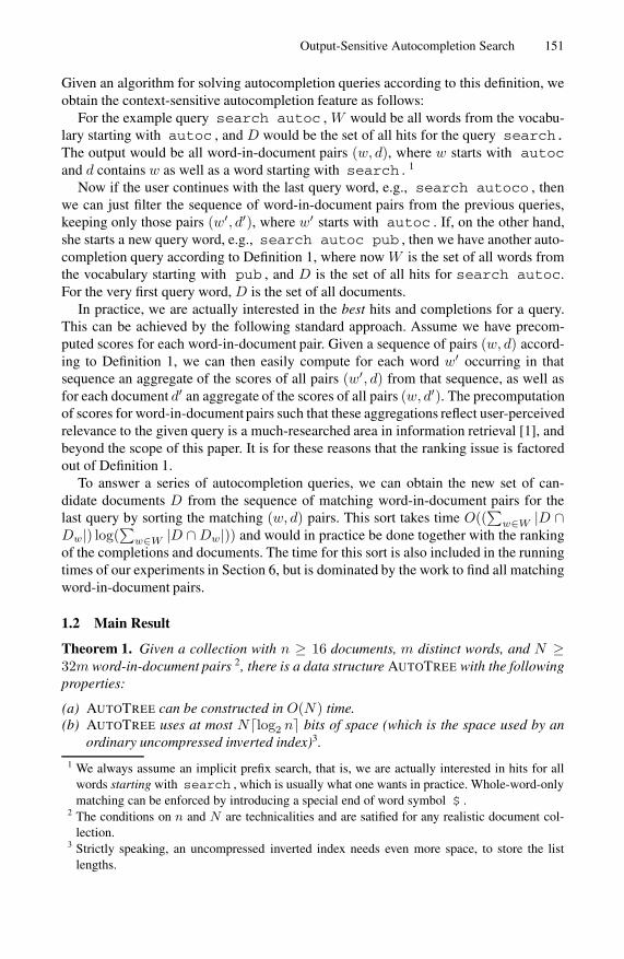
Theorem 1. Given a collection with n ≥ 16 documents, m distinct words, and N ≥32m word-in-document pairs 2, there is a data structure AUTOTREE with the followingproperties:

(a) AUTOTREE can be constructed in O(N) time.(b) AUTOTREE uses at most N�log2 n� bits of space (which is the space used by an

ordinary uncompressed inverted index)3.

1 We always assume an implicit prefix search, that is, we are actually interested in hits for allwords starting with search , which is usually what one wants in practice. Whole-word-onlymatching can be enforced by introducing a special end of word symbol $ .

2 The conditions on n and N are technicalities and are satified for any realistic document col-lection.

3 Strictly speaking, an uncompressed inverted index needs even more space, to store the listlengths.

152 H. Bast, C.W. Mortensen, and I. Weber

(c) AUTOTREE can process an autocompletion query (D, W ) in time

O((α + β)|D| +

∑

w∈W|D ∩ Dw|

),

where Dw is the set of documents containing word w. Here α = N |W |/(mn),which is bounded above by 1, unless the word range is very large (e.g., when com-pleting a single letter). If we assume that the words in a document with L words area random size-L subset of all words, β is at most 2 in expectation. In our experi-ments, β is indeed around 2 on the average and about 4 in the (rare) worst case.Our analysis implies a general worst-case bound of log(mn/N).

Note that for constant α and β the running time is asymptotically optimal, as it takesΩ(|D|) time to inspect all of D and it takes Ω(

∑w∈W |D ∩ Dw|) time to output the

result.We implemented AUTOTREE, and in Section 6 show that its processing time cor-

relates almost perfectly with the bound from Theorem 1(c) above. In that Section, wealso compare it to an inverted index, its presumably closest competitor (see Section1.4), which AUTOTREE outperforms by a factor of 10 in worst-case processing time(which is key for an interactive feature), and by a factor of 4 in average-case processingtime.

1.3 Related Work

To the best of our knowledge, the autocompletion problem, as we have defined it above,has not been explicitly studied in the literature. The problem is derived from a searchengine, which we have devised and implemented, and which is described in [2]; for alive demo, see http://search.mpi-inf.mpg.de/wikipedia. The emphasisin [2] is on usability (of the autocompletion feature) and on compressibility (of the data),and not on designing an output-sensitive algorithm. The data structures and algorithmsin [2] are completely different from those presented in this article.

The most straightforward way to process an autocompletion query (D, W ) would beto explicitly search each document from D for occurrences of a word from W . However,this would give us a non-constant query processing time per element of D, completelyindependent of the respective |W | or output size

∑w∈W |D ∩ Dw|. For these reasons,

we do not consider this approach further in this paper. Instead, our baseline in this paperis based on an inverted index, the data structure underlying most (if not all) large-scalecommercial search engines [1]; see Section 1.4.

Definition 1 looks reminiscent of multi-dimensional search problems, where the col-lections consists of tuples (of some fixed dimensionality), and queries are asking forall tuples contained in a tuple of given ranges [3,4,5,6]. Provided that we are will-ing to limit the number of query words, such data structures could indeed be used toprocess our autocompletion queries. If we want fast processing times, however, any ofthe known data structures uses space on the order of N1+d, where N is the number ofword-in-document pairs in the collection, and d grows (fast) with the dimensionality.In the description of our data structures we will point out some interesting analogies tothe geometric range-search data structures from [7] and [8].

http://search.mpi-inf.mpg.de/wikipedia


The large body of work on string searching concerned with data structures such asPAT/suffix tree/arrays [9,10] is not directly applicable to our problem. Instead, it canbe seen as orthogonal to the problem we are discussing here. Namely, in the context ofour autocompletion problem these data structures would serve to get from mere prefixsearch to full substring search. For example, our Theorem 1 could be enhanced to fullsubstring search by first building a suffix data structure like that of [10], and then build-ing our data structure on top of the sorted list of all suffixes (instead of the list of thedistinct words).

There is a large body of more applied work on algorithms and mechanisms for pre-dicting user input, for example, for typing messages with a mobile phone, for users withdisabilities concerning typing, or for the composition of standard letters [11,12,13,14].In [15], contextual information has been used to select promising extensions for a query;the emphasis of that paper is on the quality of the extensions, while our emphasis here ison efficiency. An interesting, somewhat related phrase-browsing feature has been pre-sented in [16,17]; in that work, emphasis was on the identification of frequent phrasesin a collection.

1.4 The BASIC Scheme and Outline of the Rest of the Paper

The following BASIC scheme is our baseline in this paper. It is based on the invertedindex [1], for which we simply precompute for each word from the collection the listof documents containing that word. For an efficient query processing, these lists aretypically sorted, and we assume a sorting by document number.

Having precomputed these lists, BASIC processes an autocompletion query (D, W )very simply as follows: For each word w ∈ W , fetch the list Dw of documents thatcontain w, compute the intersection D ∩ Dw, and append it to the output.

Lemma 1. BASIC uses time at least Ω(∑

w∈W min{|D|, |Dw|}) to process an auto-completion query (D, W ). The inverted lists can be stored using a total of at mostN · �log2 n� bits, where n is the total number of documents, and N is the total numberof word-in-document pairs in the collection.

Lemma 1, whose proof can be found in [18], points out the inherent problem of BASIC:its query processing time depends on the size of both |D| and |W |, and it can become|D| · |W | in the worst case.

In the following sections, we develop a new indexing scheme AUTOTREE, with theproperties given in Theorem 1. A combination of four main ideas will lead us to thisnew scheme: a tree over the words (Section 2), relative bit vectors (Section 3), pushingup the words (Section 4), and dividing into blocks (Section 5). In Section 6, we willcomplement our theoretical findings with experiments on a large test collection.

All space and time bounds are concisely stated in formal lemmas, the proofs of whichcan be found in [18].

2 Building a Tree Over the Words (TREE)

The idea behind our first scheme on the way to Theorem 1 is to increase the amountof preprocessing by precomputing inverted lists not only for words but also for their


prefixes. More precisely, we construct a complete binary tree with m leaves, where mis the number of distinct words in the collection. We assume here and throughout thepaper that m is a power of two. For each node v of the tree, we then precompute thesorted list Dv of documents which contain at least one word from the subtree of thatnode. The lists of the leaves are then exactly the lists of an ordinary inverted index, andthe list of an inner node is exactly the union of the lists of its two children. The list ofthe root node is exactly the set of all non-empty documents. A simple example is givenin Figure 1.

Fig. 1. Toy example for the data structure of scheme TREE with 10 documents and 4 differentwords

Given this tree data structure, an autocompletion query given by a word range W and aset of documents D is then processed as follows.

1. Compute the unique minimal sequence v1, . . . , v� of nodes with the property thattheir subtrees cover exactly the range of words W . Process these � nodes from leftto right, and for each node v invoke the following procedure.

2. Fetch the list Dv of v and compute the intersection D ∩ Dv. If the intersection isempty, do nothing. If the intersection is non-empty, then if v is a leaf correspondingto word w, report for each d ∈ D ∩Dv the pair (w, d). If v is not a leaf, invoke thisprocedure (step 2) recursively for each of the two children of v.

Scheme TREE can potentially save us time: If the intersection computed at an innernode v in step 2 is empty, we know that none of the words in the whole subtree of v isa completion leading to a hit, that is, with a single intersection we are able to rule out alarge number of potential completions. However, if the intersection at v is non-empty,we know nothing more than that there is at least one word in the subtree which will leadto a hit, and we will have to examine both children recursively. The following lemmashows the potential of TREE to make the query processing time depend on the outputsize instead of on W as for BASIC. Since TREE is just a step on the way to our finalscheme AUTOTREE, we do not give the exact query processing time here but just thenumber of nodes visited, because we need exactly this information in the next section.

Lemma 2. When processing an autocompletion query (D, W ) with TREE, at most2(|W ′| + 1) log2 |W | nodes are visited, where W ′ is the set of all words from W thatoccur in at least one document from D.


The price TREE pays in terms of space is large. In the worst case, each level of the treewould use just as much space as the inverted index stored at the leaf level, which wouldgive a blow-up factor of log2 m.

3 Relative Bitvectors (TREE+BITVEC)

In this section, we describe and analyze TREE+BITVEC, which reduces the space us-age from the last section, while maintaining as much as possible of its potential for aquery processing time depending on W ′, the set of matching completions, instead of onW . The basic trick will be to store the inverted lists via relative bit vectors. The result-ing data structure turns out to have similarities with the static 2-dimensional orthogonalrange counting structure of Chazelle [7].

In the root node, the list of all non-empty documents is stored as a bit vector: whenN is the number of documents, there are N consecutive bits, and the ith bit correspondsto document number i, and the bit is set to 1 if and only if that document contains atleast one word from the subtree of the node. In the case of the root node this means thatthe ith bit is 1 if and only if document number i contains any word at all.

Now consider any one child v of the root node, and with it store a vector of N ′

bits, were N ′ is the number of 1-bits in the parent’s bit vector. To make it interestingalready at this point in the tree, assume that indeed some documents are empty, so thatnot all bits of the parent’s bit vector are set to one, and N ′ < N . Now the jth bit ofv corresponds to the jth 1-bit of its parent, which in turn corresponds to a documentnumber ij . We then set the jth bit of v to 1 if and only if document number ij containsa word in the subtree of v.

The same principle is now used for every node v that is not the root. Constructingthese bit vectors is relatively straightforward; it is part of the construction given inAppendix A.

Fig. 2. The data structure of TREE+BITVEC for the toy collection from Figure 1

Lemma 3. Let stree denote the total lengths of the inverted lists of algorithm TREE.The total number of bits used in the bit vectors of algorithm TREE+BITVEC is then atmost 2stree plus the number of empty documents (which cost a 0-bit in the root each).

The procedure for processing a query with TREE+BITVEC is, in principle, the same asfor TREE. The only difference comes from the fact that the bit vectors, except that ofthe root, can only be interpreted relative to their respective parents.


To deal with this, we ensure that whenever we visit a node v, we have the set Iv ofthose positions of the bit vector stored at v that correspond to documents from the givenset D, as well as the |Iv| numbers of those documents. For the root node, this is trivial tocompute. For any other node v, Iv can be computed from its parent u: for each i ∈ Iu,check if the ith bit of u is set to 1, if so compute the number of 1-bits at positions lessthan or equal to i, and add this number to the set Iv and store by it the number of thedocument from D that was stored by i. With this enhancement, we can follow the samesteps as before, except that we have to ensure now that whenever we visit a node that isnot the root, we have visited its parent before. The lemma below shows that we have tovisit an additional number of up to 2 log2 m nodes because of this.

Lemma 4. When processing an autocompletion query (D, W ) with TREE+BITVEC,at most 2(|W ′| + 1) log2 |W | + 2 log2 m nodes are visited, with W ′ defined as inLemma 2.

4 Pushing Up the Words (TREE+BITVEC+PUSHUP)

The scheme TREE+BITVEC+PUSHUP presented in this section gets rid of the log2|W | factor in the query processing time from Lemma 4. The idea is to modify theTREE+BITVEC data structure such that for each element of a non-empty intersection,we find a new word-in-document pair (w, d) that is part of the output. For that we storewith each single 1-bit, which indicates that a particular document contains a word froma particular range, one word from that document and that range. We do this in such away that each word is stored only in one place for each document in which it occurs.When there is only one document, this leads to a data structure that is similar to thepriority search tree of McCreight, which was designed to solve the so-called 3-sideddynamic orthogonal range-reporting problem in two dimensions [8].

Let us start with the root node. Each 1-bit of the bit vector of the root node corre-sponds to a non-empty document, and we store by that 1-bit the lexicographically small-est word occurring in that document. Actually, we will not store the word but rather itsnumber, where we assume that we have numbered the words from 0, . . . , m − 1.

More than that, for all nodes at depth i (i.e., i edges away from the root), we omitthe leading i bits of its word number, because for a fixed node these are all identicaland can be computed from the position of the node in the tree. However, asympoticallythis saving is not required for the space bounds in Theorem 1 as dividing the wordsinto blocks will already give a sufficient reduction of the space needed for the wordnumbers.

Now consider anyone child v of the root node, which has exactly one half H ofall words in its subtree. The bit vector of v will still have one bit for each 1-bit of itsparent node, but the definition of a 1-bit of v is slightly different now from that forTREE+BITVEC. Consider the jth bit of the bit vector of v, which corresponds to thejth set bit of the root node, which corresponds to some document number ij . Then thisdocument contains at least one word — otherwise the jth bit in the root node wouldnot have been set — and the number of the lexicographically smallest word containedis stored by that jth bit. Now, if document ij contains other words, and at least one ofthese other words is contained in H , only then the jth bit of the bit vector of v is set


to 1, and we store by that 1-bit the lexicographically smallest word contained in thatdocument that has not already been stored in one of its ancestors (here only the rootnode).

Figure 3 explains this data structure by a simple example. The construction of thedata structure is relatively straightforward and can be done in time O(N). Details aregiven in Appendix A.

Fig. 3. The data structure of TREE+BITVEC+PUSHUP for the example collection from Figure1. The large bitvector in each node encodes the inverted list. The words stored by the 1-bits ofthat vector are shown in gray on top of the vector. The word list actually stored is shown belowthe vector, where A=00, B=01, C=10, D=11, and for each node the common prefix is removed,e.g., for the node marked C-D, C is encoded by 0 and D is encoded by 1. A total of 49 bits isused, not counting the redundant 000 vectors and bookkeeping information like list lengths etc.

To process a query we start at the root. Then, we visit nodes in such an order thatwhenever we visit a node v, we have the set Iv of exactly those positions in the bitvector of v that correspond to elements from D (and for each i ∈ Iv we know itscorresponding element di in D). For each such position with a 1-bit, we now checkwhether the word w stored by that 1-bit is in W , and if so output (w, di). This can beimplemented by random lookups into the bit vector in time O(|Iv |) as follows. First,it is easy to intersect D with the documents in the root node, because we can simplylookup the document numbers in the bitvector at the root. Consider then a child v of theroot. What we want to do is to compute a new set Iv of document indices, which givesthe numbering of the document indices of D in terms of the numbering used in v. Thisamounts to counting the number of 1-bits in the bitvector of v up to a given sequence ofindices. Each of these so-called rank computations can be performed in constant timewith an auxiliary data structure that uses space sublinear in the size of the bitvector [19].

Consider again the check whether a word w stored by a 1-bit corresponding to adocument from D is actually in W . This check can only fail for relatively few nodes,namely those with a least one leaf not from W in their subtree. These checks do notcontribute an element to the output set, and are accounted for by the factor β mentionedin Theorem 1, and Lemmas 5 and 7 below.

Lemma 5. With TREE+BITVEC+PUSHUP, an autocompletion query (D, W ) can beprocessed in time O

(|D| · β +

∑w∈W |D ∩ Dw|

), where β is bounded by log2 m as

well as by the average number of distinct words in a document from D. For the specialcase, where W is the range of all words, the bound holds with β = 1.


Lemma 6. The bit vectors of TREE+BITVEC+PUSHUP require a total of at most2N + n bits. The auxiliary data structure (for the constant-time rank computation)requires at most N bits.

5 Divide into Blocks (TREE+BITVEC+PUSHUP+BLOCKS)

This section is our last station on the way to our main result, Theorem 1.For a given B, with 1 ≤ B ≤ m, we divide the set of all words in blocks of equal

size B. We then construct the data structure according to TREE+BITVEC+PUSHUPfor each block separately. As we only have to consider those blocks, which contain anywords from W , this gives a further speedup in query processing time. An autocomple-tion query given by a word range W and a set of documents D is then processed in thefollowing three steps.

1. Determine the set of � (consecutive) blocks, which contain at least one word fromW , and for i = 1, . . . , �, compute the subrange Wi of W that falls into block i.Note that W = W1∪ · · · ∪W�.

2. For i = 1, . . . , �, process the query given by Wi and D according to TREE+BITVEC+ PUSHUP, resulting in a set of matches Mi := {(w, d) ∈ C : w ∈Wi, d ∈ D}, where C is the set of of word-in-document pairs.

3. Compute the union of the sets of matching word-in-document pairs ∪�i=1Mi (a

simple concatenation).

Lemma 7. With TREE+BITVEC+PUSHUP+BLOCKS and block size B, an autocom-pletion query (D, W ) can be processed in time O

(|D| · (α + β) +

∑w∈W |D ∩ Dw|

),

where α = |W |/B and β is bounded by log2 B as well as by the average number ofdistinct words from W1 ∪W� (the first and the last subrange from above) in a documentfrom D.

Lemma 8. TREE+BITVEC+PUSHUP+BLOCKS with block size B requires at most3N +n·�m/B� bits for its bit vectors and at most N�log2 B� bits for the word numbersstored by the 1-bits. For B ≥ mn/N , this adds up to at most N(4 + �log2 B�) bits.

Part (a) of Theorem 1 is established by the construction given in Appendix A. Part (b)of Theorem 1 follows from Lemma 8 by choosing B = �nm/N�. This choice of Bminimizes the space bound of Lemma 8, and we call the corresponding data structureAUTOTREE. Part (c) of Theorem 1 follows from Lemma 7 and the following remarks.If the words in a document with L words are a random size-L subset of all words, thenthe average number of words per document that fall into a fixed block is at most 1. Inour experiments, the average value for β was 2.2. For the exact definition of β, see [18].

6 Experiments

We tested both AUTOTREE and our baseline BASIC on the corpus of the TREC 2004Robust Track (ROBUST ’04), which consists of the documents on TREC disks 4 and


5, minus the Congressional Record [20]. We implemented AUTOTREE with a blocksize of 4096, which is the optimal block size according to Section 5, rounded to thenearest power of two. The following table gives details on the collection and on thespace consumption of the two schemes; as we can see, AUTOTREE does indeed use nomore space (and for this collection, in fact, significantly less) than BASIC, as guaranteedby Theorem 1.

Table 1. The characteristics of our test collection: n = number of documents, m = number ofdistinct words, N/n = average number of distinct words in a document, B∗ = space-optimalchoice for the block size. The last two columns give the space usage of BASIC and AUTOTREE

in bits per word-in-document pair.

bits per word-in-doc pair

Collection raw size n m N/n B∗ BASIC AUTOTREE

ROBUST ’04 1,904 MB 528,025 771,189 219.2 4,096 19.0 13.9

Queries are derived from the 200 “old” 4 queries (topics 301-450 and 601-650) of theTREC Robust Track in 2004 [20], by “typing” these queries from left to right, takinga minimum word length of 4 for the first query word, and 2 for any query word afterthe first. From these autocompletion queries we further omitted those, which wouldbe obtained by simple filtering from a prefix according to the explanation followingDefinition 1. This filtering procedure is identical for AUTOTREE and BASIC and takesonly a small fraction of the time for the autocompletion queries processed according toDefinition 1, which is why we omitted it from consideration in our experiments. To givean example, for the ad hoc query world bank criticism , we considered theautocompletion queries worl , world ba , and world bank cr . We considereda total number of 512 such autocompletion queries.

We implemented BASIC and AUTOTREE in C++ and measured query processingtimes on a Dual Opteron machine, with 2 Intel Xeon 3 GHz processors, 8 GB of mainmemory, running Linux. We measured the time for producing the output according toDefinition 1. The time for scoring and ranking would be identical for AUTOTREE andBASIC, and would, according to a number of tests, take only a small fraction of theaforementioned processing time. We therefore excluded it from our measurements. ForBASIC, we implemented a fast linear-time intersect, which, on average, turned out to befaster than its asymptotically optimal relatives [21].

The results from Table 2 conform nicely to our theoretical analysis. Four main ob-servations can be made: (i) with respect to maximal query processing time, which iskey for an interactive application, AUTOTREE improves over BASIC by a factor of 10;(ii) in average processing time, which is significant for throughput in a high-load sce-nario, the improvement is still a factor of 4; (iii) processing times of AUTOTREE aresharply concentrated around their mean, while for BASIC they vary widely (in both di-rections as we checked); (iv) the almost perfect correlation between query processingtimes and our analytical bounds (explained in the caption of Figure 2) demonstrates

4 They are “old” as they had been used in previous years for TREC.


Table 2. Processing times statistics of BASIC and AUTOTREE for all 512 autocompletion queries.The 6th and 7th column show the kth worst processing time, where k is 10% and 5%, respectively,of the number of queries. The last column gives the correlation factor between query processingtimes and total list volume

�w∈W (|D| + |Dw |) for BASIC, and input size plus total output

volume |D| + 5�

w∈W |D ∩ Dw | for AUTOTREE.

Scheme Max Mean StdDev Median 90%-ile 95%-ile Correlation

BASIC 6.32secs 0.19secs 0.55secs 0.034secs 0.41secs 0.93secs 0.996

AUTOTREE 0.63secs 0.05secs 0.06secs 0.028secs 0.11secs 0.14secs 0.973

Table 3. Breakdown of query processing for BASIC and AUTOTREE by number of query words

1-word multi-word

Scheme Max Mean Max Mean

BASIC 0.10secs 0.01secs 6.32secs 0.30secs

AUTOTREE 0.37secs 0.09secs 0.63secs 0.02secs

both the soundness of our theoretical modelling and analysis as well as the accuracy ofour implementation.

Table 3, finally, breaks down query processing times by the number of query words.As we can see, BASIC is significantly faster than AUTOTREE for the 1-word queries,however, not because AUTOTREE is slow, but because BASIC is extremely fast on thesequeries. This is so, because BASIC does not have to compute any intersections for 1-query but merely has to copy all relevant lists Dw to the output, whereas AUTOTREE

has to extract, for each output element, bits from its (packed) document id and wordid vectors. On multi-word queries, BASIC has to process a much larger volume thanAUTOTREE, and we see essentially the situation discussed above for the overall figures.

References

1. Witten, I.H., Bell, T.C., Moffat, A.: Managing Gigabytes: Compressing and Indexing Docu-ments and Images, 2nd edition. Morgan Kaufmann (1999)

2. Bast, H., Weber, I.: Type less, find more: Fast autocompletion search with a succinct index.In: 29th Conference on Research and Development in Information Retrieval (SIGIR’06).(2006)

3. Gaede, V., Gunther, O.: Multidimensional access methods. ACM Computing Surveys 30(2)(1998) 170–231

4. Arge, L., Samoladas, V., Vitter, J.S.: On two-dimensional indexability and optimal rangesearch indexing. In: 18th Symposium on Principles of database systems (PODS’99). (1999)346–357

5. Ferragina, P., Koudas, N., Muthukrishnan, S., Srivastava, D.: Two-dimensional substringindexing. Journal of Computer and System Science 66(4) (2003) 763–774


6. Alstrup, S., Brodal, G.S., Rauhe, T.: New data structures for orthogonal range searching. In:41st Symposium on Foundations of Computer Science (FOCS’00). (2000) 198–207

7. Chazelle, B.: A functional approach to data structures and its use in multidimensional search-ing. SIAM Journal on Computing 17(3) (1988) 427–462

8. McCreight, E.M.: Priority search trees. SIAM Journal on Computing 14(2) (1985) 257–2769. Grossi, R., Vitter, J.S.: Compressed suffix arrays and suffix trees with applications to text

indexing and string matching (extended abstract). In: 32nd Symposium on the Theory ofComputing (STOC’00). (2000) 397–406

10. Ferragina, P., Grossi, R.: The string B-tree: a new data structure for string search in externalmemory and its applications. Journal of the ACM 46(2) (1999) 236–280

11. Jakobsson, M.: Autocompletion in full text transaction entry: a method for humanized input.In: Conference on Human Factors in Computing Systems (CHI’86). (1986) 327–323

12. Darragh, J.J., Witten, I.H., James, M.L.: The reactive keyboard: A predictive typing aid.IEEE Computer (1990) 41–49

13. Stocky, T., Faaborg, A., Lieberman, H.: A commonsense approach to predictive text entry.In: Conference on Human Factors in Computing Systems (CHI’04). (2004) 1163–1166

14. Bickel, S., Haider, P., Scheffer, T.: Learning to complete sentences. In: 16th EuropeanConference on Machine Learning (ECML’05). (2005) 497–504

15. Finkelstein, L., Gabrilovich, E., Matias, Y., Rivlin, E., Solan, Z., Wolfman, G., Ruppin, E.:Placing search in context: The concept revisited. In: 10th World Wide Web Conference(WWW’10). (2001) 406–414

16. Paynter, G.W., Witten, I.H., Cunningham, S.J., G., G.B.: Scalable browsing for large collec-tions: A case study. In: 5th Conference on Digital Libraries (DL’00). (2000) 215–223

17. Nevill-Manning, C.G., Witten, I., Paynter, G.W.: Lexically-generated subject hierarchies forbrowsing large collections. International Journal of Digital Libraries 2(2/3) (1999) 111–123

18. Bast, H., Mortensen, C.W., Weber, I.: Output-sensitive autocompletion search. Techni-cal Report 1–007 (2006) See first author’s website http://www.mpi-inf.mpg.de/˜bast/publications.html.

19. Munro, J.I.: Tables. In: 16th Conference on Foundations of Software Technology and Theo-retical Computer Science (FSTTCS’96). (1996) 37–42

20. Voorhees, E.: Overview of the trec 2004 robust retrieval track. In: 13th Text Retrieval Confer-ence (TREC’04). (2004) http://trec.nist.gov/pubs/trec13/papers/ROBUST.OVERVIEW.pdf.

21. Demaine, E.D., Lopez-Ortiz, A., Munro, J.I.: Adaptive set intersections, unions, and differ-ences. In: 11th Symposium on Discrete Algorithms (SODA’00). (2000) 743–752

A The Index Construction for TREE+BITVEC+PUSHUP

In this appendix we describe the construction of the index for TREE+BITVEC+PUSHUP. Full proofs of Lemmas 2, 3, 4, 5, 6, 7, and 8 can be found in [18].

The construction of the tree for algorithm TREE+BITVEC+PUSHUP is relativelystraightforward and takes constant amortized time per word-in-document occurrence(assuming each document contains its word sorted in ascending order).

1. Process the documents in order of ascending document numbers, and for each doc-ument d do the following.

2. Process the distinct words in document d in order of ascending word number, andfor each word w do the following. Maintain a current node, which we initialize asan artificial parent of the root node.

http://www.mpi-inf.mpg.de/~bast/publications.html

http://www.mpi-inf.mpg.de/~bast/publications.html


3. If the current node does not contain w in its subtree, then set the current node toits parent, until it does contain w in its subtree. For each node left behind in thisprocess, append a 0-bit to the bit vector of those of its children which have not beenvisited.Note: for a particular word, this operation may take non-constant time, but oncewe go from a node to its parent in this step, the old node will never be visited again.Since we only visit nodes, by which a word will be stored and such nodes are visitedat most three times, this gives constant amortized time for this step.

4. Set the current node to that one child which contains w in its subtree. Store theword w by this node. Add a 1-bit to the bit vector of that node.

Documents

Output-Sensitive Autocompletion Search