Embed Size (px)
Citation preview

Output Dynamics In the Long Run: Issues of EconomicGrowth
Mausumi Das
Lecture Notes, DSE
April 12-25; 2016
Das (Lecture Notes, DSE) Economic Growth April 12-25; 2016 1 / 148
Output Dynamics: Short Run to Long Run
In the first module of the course, we have seen how output andemployment are determined in the short run.
In the Classical system (and its various extensions), these aredetermined by the supply side factors (production conditions); role ofdemand is limited to the detemination of the equilibrium price level.
In the Keynesian system (and its various extensions), aggregatedemand plays a direct role in determining equilibrium output andemployment in the short run.
As discussed before, both these systems are based on aggregativebehavioural equations.
One could provide micro-founded justifications for some of theseequations, but they may not necessarily be consistent with oneanother.
Das (Lecture Notes, DSE) Economic Growth April 12-25; 2016 2 / 148
Output Dynamics: Short Run to Long Run (Contd.)
Alternatively, one could build an internally consistent, dynamicgeneral equilibrium (DGE) framework, where forward-looking agentsmake their optimal decisions, taking both current and future variablesinto account.
But this would entail dynamic equations involving today’s andtomorrow’s consumption; today’s and tomorrow’s capital stock etc.
In other words this would bring us directly into the realm of outputdyamics over time, i.e., economic growth.
In the third module, we are going to explore issues pertaining to theoutput dynamics over time.
In particular, we shall examine how the period-by-period outputdynamics generate a growth path for the economy and what happensto this growth trajectory in the long run:
Does the economy reach a long run equilibrium with a constant growthrate, or does growth fizzle out in the long run?
Das (Lecture Notes, DSE) Economic Growth April 12-25; 2016 3 / 148
Definition of Long Run: Steady State vis-a-vis BalancedGrowth Path
Before we proceed further, it is important to define the concept of‘long run equilibrium’in the context of growth models.
Long run equilibrium in a growth model is typically defined as abalanced growth path, where all endogeneous variables grow atsome constant rate.
This constant growth rate may differ from variable to variable.
More importantly, this constant growth rate could even be zero forsome variables.
The latter case is typically identified as the steady state in theconventional dynamic analysis (which is a special case of a balancedgrowth path).
Das (Lecture Notes, DSE) Economic Growth April 12-25; 2016 4 / 148
Output Dynamics: Short Run to Long Run (Contd.)
Must growth dynamics be necessarily based on the DGE framework?
In other words, can the aggregative behavioural equations of theKeynesian or the Classical system also throw up some growthtrajectories for the economy?
If yes, how would they differ from the growth trajectories predicted bythe DGE framework?
Indeed, one can develop growth models based on the short run(static) characterization of the macroeconomy in either the Keynesiansystem or the Classical system.
And the long run charateristics of these growth models may differsubstantially from that of the DGE framework.
We start our discussion by analysing the dynamic versions of theseaggregative models.
Das (Lecture Notes, DSE) Economic Growth April 12-25; 2016 5 / 148

Keynesian System: Short Run to Long Run
The dynamic extension of the Keynesian system was developedindependently by Roy Harrod (1939) and Evsey Domar (1946).We shall focus on Harrod’s version.It is a Keynesian system - so equilibrium output in the short run isdetermined by the level of aggregate demand.We shall abstract away from money, interest and prices and assume avery simple structure where aggregate demand consists only ofconsumption demand and investment demand:
Yt ≡ ADt = Ct + It .Consumption function is Keynesian: people consume a fixedproportion of their income and save the rest:
Ct = (1− s)Yt ; 0 < s < 1,
where s is the constant marginal propensity to save (determinedexogenously).
Das (Lecture Notes, DSE) Economic Growth April 12-25; 2016 6 / 148
A Keynesian Demand-driven Growth Model: Harrod
For any given level of investment It , we can then derive the short runequilibrium output in this simple Keynesian model as:
Yt ≡ ADt =Its. (1)
In the static simple Keynesian model, of course, investment (I ) isassumed to be autonomous.
In this dynamic model it is likely to change over time.
How exactly does it change over time? What are the factors thatdetermine the investment level?
These are important questions that we shall take up in a moment.
But before that, let us discuss the production side of the story.
Das (Lecture Notes, DSE) Economic Growth April 12-25; 2016 7 / 148

Harrod Model: Production Side Story
Production is carried out by firms using a production function thatuses capital and labour as inputs.
Summing over all firms, we get the aggregate production function as:
Ot = F (Kt ,Nt )
where Kt denotes the total available stock of capital and Nt denotesthe existing working population in the economy.
The characteristics of the production function F are determined bythe existing technology and will be specified below.
But notice that aggregate supply is determined by technologicalconditions, while aggregate demand is determined by the amount ofinvestment and the savings propensity.
So there is no apriori reason for the two to be equal (unless bychance).
Das (Lecture Notes, DSE) Economic Growth April 12-25; 2016 8 / 148
Harrod Model: Production Side Story (Contd.)
What happens when the two are not equal?
Typically in the macro literature there are three types of adjustments:(a) the price level adjusts (and to the extent that aggregate demandand aggreagte supply respond to price level, they are eventuallyequalized);(b) the adjustment takes place in terms of unintended inventoryaccumulation or decumulation, i.e., the producers produce at fullcapacity but if the production is in excess of demand then the extragoes to the inventory stock (opposite happens when production fallsshort of demand);(c) the adjustment takes place directly in terms of less than fullcapacity utilization of the existing factors, i.e, producers, anticipatingexcess supply, cut back on usage of Kt and Nt (or anticipating excessdemand, overstretch the use of existing factors - assuming that isfeasible).
Das (Lecture Notes, DSE) Economic Growth April 12-25; 2016 9 / 148
Harrod Model: Production Side Story (Contd.)
Now this is a Keynesian model where prices are rigid. So the firstchannel of adjustment is ruled out.
Here we shall assume that whenever there is a mismatch betweendemand and supply, the adjustment happens through the stockof inventories.(This assumption is not critical. One could easily construct ademand-driven growth model where adjsutment is done throughcapacity utilization. The results would be qualitatively similar.)
ThusOt ≡ ASt = F (Kt ,Nt ).
Since the excess supply/demand is adjusted via the inventories,inventory stock evolves over time according to the following rule:
Vt+1 = Vt + (Ot − Yt ). (2)
Das (Lecture Notes, DSE) Economic Growth April 12-25; 2016 10 / 148

Harrod Model: Production Side Story (Contd.)
Now let us look at the specific production function used by Harrod.
Harrod assumed a fixed coeffi cient production technology such that
F (Kt ,Nt ) = Min[Ktα,Ntβ
],
where α, β > 0 are technology determined parameters, representingthe inverse of capital productivity and labour productivity respectively.
The fixed coeffi cient production function has important implicationsfor factor utilization.
Recall the the economy has certain historically given stocks of capital(Kt) and labour (Kt) at the beginning of period t.
Given these stocks, it is unlikely thatKtα=Ntβat every t.
Thus one of the factors is likely to be underutilized.
Das (Lecture Notes, DSE) Economic Growth April 12-25; 2016 11 / 148
Harrod Model: Production Side Story (Contd.)
We shall call an economy ‘capital-constrained’(or, equivalently,
‘labour-surplus’) iffKtα<Ntβ.
Similarly, we shall call an economy ‘labour-constrained’(or,
equivalently, ‘capital-surplus’) iffKtα>Ntβ.
Harrod assumed that the economy is ‘capital-constrained’, at leastto begin with.
This implies that production and aggregate supply in this economy isdetermined by the following equation:
Ot ≡ ASt =Ktα. (3)
Das (Lecture Notes, DSE) Economic Growth April 12-25; 2016 12 / 148
Harrod Model: Production Side Story (Contd.)
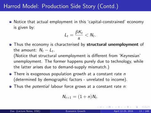
Notice that actual employment in this ‘capital-constrained’economyis given by:
Lt =βKt
α< Nt .
Thus the economy is characterised by structural unemployment ofthe amount: Nt − Lt .(Notice that structural unemployment is different from ‘Keynesian’unemployment. The former happens purely due to technology, whilethe latter arises due to demand-supply mismatch.)
There is exogenous population growth at a constant rate n(determined by demographic factors - unrelated to income).
Thus the potential labour force grows at a constant rate n:
Nt+1 = (1+ n)Nt .
Das (Lecture Notes, DSE) Economic Growth April 12-25; 2016 13 / 148
Harrod Model: Factor Returns
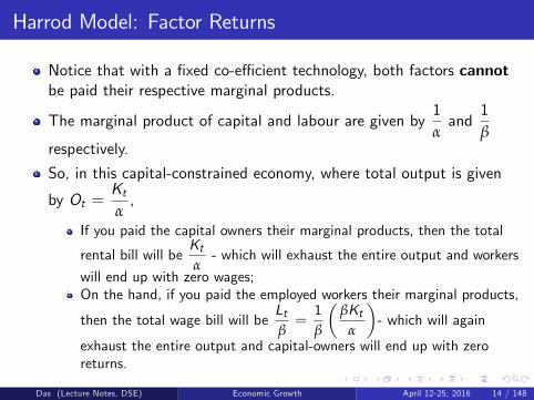
Notice that with a fixed co-effi cient technology, both factors cannotbe paid their respective marginal products.
The marginal product of capital and labour are given by1αand
1β
respectively.
So, in this capital-constrained economy, where total output is given
by Ot =Ktα,
If you paid the capital owners their marginal products, then the total
rental bill will beKtα- which will exhaust the entire output and workers
will end up with zero wages;On the hand, if you paid the employed workers their marginal products,
then the total wage bill will beLtβ=1β
(βKt
α
)- which will again
exhaust the entire output and capital-owners will end up with zeroreturns.
Das (Lecture Notes, DSE) Economic Growth April 12-25; 2016 14 / 148

Harrod Model: Factor Returns (Contd.)
Thus the usual assumption about factor returns being equal to theirrespective marginal products would not work here.
The factor returns must be determined exogenously - by norms,conventions, labour unions etc.
Here we shall assume that the real wage is fixed exogeneously at some
given level ω <1β.
The rest of the output is distributed residually to the capital ownersas rents/profits.
Das (Lecture Notes, DSE) Economic Growth April 12-25; 2016 15 / 148

Harrod Model: The Investment Function
The most important assumption in the Harrod model is the existenceof an independent investment function, which depends on producers’expectations about future demand.
Typically, in supply-driven growth models (e.g., Neoclassical andothers), it is assumed that there is no independent investmentfunction and all savings are automatically invested - which makessavings and investment always identical.It also implies that both savings and investment decisions are madeby the households.
Harrod on the other hand was highlighting the fact that savings andinvestment decisions are separate: savings decisions are undertaken byhouseholds, while investment decisions are made by producers.
Allowing for this dichotomy plays a very important role in the Harrodmodel - as we shall soon see.
Das (Lecture Notes, DSE) Economic Growth April 12-25; 2016 16 / 148
Harrod Model: The Investment Function (Contd.)
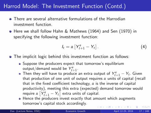
There are several alternative formulations of the Harrodianinvestment function.
Here we shall follow Hahn & Mathews (1964) and Sen (1970) inspecifying the following investment function:
It = α [Y et+1 − Yt ] . (4)
The implicit logic behind this investment function as follows:
Suppose the producers expect that tomorrow’s equilibriumoutput/demand would be Y et+1.Then they will have to produce an extra output of Y et+1 − Yt . Giventhat production of one unit of output requires α units of capital (recallthat in the fixed coeffi cient technology, α is the inverse of capitalproductivity), meeting this extra (expected) demand tomorrow wouldrequire α
[Y et+1 − Yt
]extra units of capital.
Hence the producers invest exactly that amount which augmentstomorrow’s capital stock accordingly.
Das (Lecture Notes, DSE) Economic Growth April 12-25; 2016 17 / 148
Harrod Model: The Investment Function (Contd.)
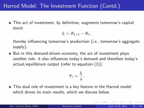
This act of investment, by definition, augments tomorrow’s capitalstock:
It = Kt+1 −Kt ,thereby influencing tomorrow’s production (i.e., tomorrow’s aggregatesupply).
But in this demand-driven economy, the act of investment playsanother role: it also influences today’s demand and therefore today’sactual/equilibrium output (refer to equation (1)):
Yt =Its.
This dual role of investment is a key feature in the Harrod modelwhich drives its main results, which we discuss below.
Das (Lecture Notes, DSE) Economic Growth April 12-25; 2016 18 / 148

Output Dynamics in the Harrod Model & the AssociatedGrowth Path:
Recall that in this economy,
Yt ≡ ADt =α[Y et+1 − Yt
]s
=Kt+1 −Kt
s, (1a)
while
Ot ≡ ASt =Ktα. (2a)
There is no reason why ADt = ASt in every period. And ifADt 6= ASt , then the stock of inventories adjust.We shall analyse the growth path of the equilibrium output (Yt)under two scenarios:
Scenario I: ADt = ASt at every t (by some freak co-incidence);Scenario II: ADt 6= ASt at least at t = 0.In this latter case, we would also like to know whether in the long run(as t → ∞), the AS and AD will eventually converge to each other orwhether they will remain perpetually mismatched.
Das (Lecture Notes, DSE) Economic Growth April 12-25; 2016 19 / 148

Output Dynamics in the Harrod Model: Scenario I
Under Scenario I: Yt = Ot for every t (by assumption).Then from (1a) and (2a),
Kt+1 −Kts
=Ktα
⇒ Kt+1 −KtKt
=sα≡ g ∗ (say).
It is easy to verify that in this scenario Yt , Ot , Lt - all will grow atthe same constant growth rate (g ∗) as Kt .
Harrod called this secnario the warranted or desirable scenario (sincethere is no mismatch between AD and AS). Correspndingly, g ∗ iscalled the ‘warranted growth rate’.Notice that this scenario also represents a ‘long run equilibrium’or a‘balanced growth path’because all variables in the economy growat constant rates.
Das (Lecture Notes, DSE) Economic Growth April 12-25; 2016 20 / 148

Output Dynamics in the Harrod Model: Scenario I
A Question:Scenario I assumes that Yt = Ot in every time period (bycoincidence). Suppose the economy to begin with starts with ascenario such that Y0 = O0. Does it necessarily imply that Yt = Otfor all subsequent t?
Das (Lecture Notes, DSE) Economic Growth April 12-25; 2016 21 / 148
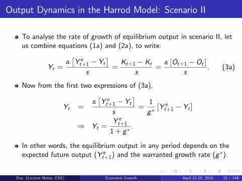
Output Dynamics in the Harrod Model: Scenario II
To analyse the rate of growth of equilibrium output in scenario II, letus combine equations (1a) and (2a), to write:
Yt =α[Y et+1 − Yt
]s
=Kt+1 −Kt
s=
α [Ot+1 −Ot ]s
. (3a)
Now from the first two expressions of (3a),
Yt =α[Y et+1 − Yt
]s
=1g ∗[Y et+1 − Yt ]
⇒ Yt =Y et+11+ g ∗
.
In other words, the equilibrium output in any period depends on theexpected future output (Y et+1) and the warranted growth rate (g
∗).
Das (Lecture Notes, DSE) Economic Growth April 12-25; 2016 22 / 148

Output Dynamics in the Harrod Model: Scenario II(Contd.)
From the above relationship, the rate of growth of equilibrium outputcan be written as follows:
gt ≡Yt+1 − Yt
Yt=Y et+2 − Y et+1
Y et+1≡ g et+1. (A)
In other words, the rate of growth of equilibrium output today isdetermined by the rate of growth of expected output tomorrow.
This begs the following question: what determines g et+1?
This will require some theory about expectation formation.
We shall discuss below some specific expectation formation rules andtheir growth implications.
But before that let us examine the rate of growth of aggrerate supplyunder scenario II.
Das (Lecture Notes, DSE) Economic Growth April 12-25; 2016 23 / 148
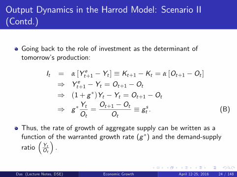
Output Dynamics in the Harrod Model: Scenario II(Contd.)
Going back to the role of investment as the determinant oftomorrow’s production:
It = α [Y et+1 − Yt ] ≡ Kt+1 −Kt = α [Ot+1 −Ot ]⇒ Y et+1 − Yt = Ot+1 −Ot⇒ (1+ g ∗)Yt − Yt = Ot+1 −Ot
⇒ g ∗YtOt=Ot+1 −Ot
Ot≡ g st . (B)
Thus, the rate of growth of aggregate supply can be written as afunction of the warranted growth rate (g ∗) and the demand-supply
ratio(YtOt
).
Das (Lecture Notes, DSE) Economic Growth April 12-25; 2016 24 / 148

Output Dynamics under Scenario II: Various ExpectationFormation Rules
Let us now examine how g et+1 is determined under various expectationformation rules.
We start with constant expectation, such that g et+1 remains constant(at some arbitrary value) for all points of time. Then there are threepossibilities.
1. Constant Expectations - Case 1: g et+1 = g∗
The rate of growth of equilibrium output is now determined triviallyfrom (A):
gt = g ∗.
But we are also interested to know what happens to thedemand-supply gap in the long run.
Das (Lecture Notes, DSE) Economic Growth April 12-25; 2016 25 / 148

Output Dynamics under Scenario II: ConstantExpectations - Case 1
Notice that under scenario II, by assumption, the economy starts with
some initial mismatch between demand and supply, i.e.,Y0O06= 1.
The question is, no matter what the initial(Y0O0
)is, does
YtOt
converge to unity in the long run?
To answer this question, let us examine the evolution of theYtOt
ratio,
or equivalently, theOtYt
ratio under case 1.
Das (Lecture Notes, DSE) Economic Growth April 12-25; 2016 26 / 148
Output Dynamics under Scenario II: ConstantExpectations - Case 1 (Contd.)
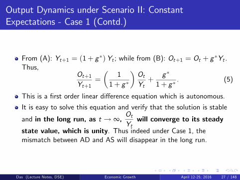
From (A): Yt+1 = (1+ g ∗)Yt ; while from (B): Ot+1 = Ot + g ∗Yt .Thus,
Ot+1Yt+1
=
(1
1+ g ∗
)OtYt+
g ∗
1+ g ∗. (5)
This is a first order linear difference equation which is autonomous.
It is easy to solve this equation and verify that the solution is stable
and in the long run, as t → ∞,OtYt
will converge to its steady
state value, which is unity. Thus indeed under Case 1, themismatch between AD and AS will disappear in the long run.
Das (Lecture Notes, DSE) Economic Growth April 12-25; 2016 27 / 148
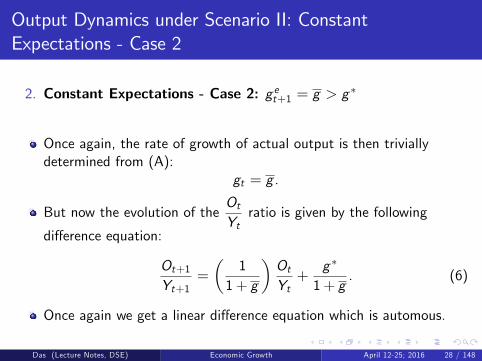
Output Dynamics under Scenario II: ConstantExpectations - Case 2
2. Constant Expectations - Case 2: g et+1 = g > g∗
Once again, the rate of growth of actual output is then triviallydetermined from (A):
gt = g .
But now the evolution of theOtYt
ratio is given by the following
difference equation:
Ot+1Yt+1
=
(1
1+ g
)OtYt+
g ∗
1+ g. (6)
Once again we get a linear difference equation which is automous.
Das (Lecture Notes, DSE) Economic Growth April 12-25; 2016 28 / 148

Output Dynamics under Scenario II: ConstantExpectations - Case 2 (Contd.)
It is easy to verify that now the steady state value is given byg ∗
g< 1,
which is once again stable.
Thus in the long run, as t → ∞,OtYt
will converge to a value
which is less than unity.Thus under Case 2, the mismatch between AD and AS does notdisappear in the long run.
In fact in the long run there is perpetual excess demand!
This would of course lead to a perpetual depletion in inventorystocks. What happens when the entire inventory stock getsexhausted? We shall come back to this issue later.
Das (Lecture Notes, DSE) Economic Growth April 12-25; 2016 29 / 148
Output Dynamics under Scenario II: ConstantExpectations - Case 3
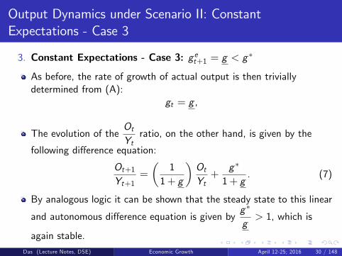
3. Constant Expectations - Case 3: g et+1 = g < g∗
As before, the rate of growth of actual output is then triviallydetermined from (A):
gt = g ,
The evolution of theOtYt
ratio, on the other hand, is given by the
following difference equation:
Ot+1Yt+1
=
(1
1+ g
)OtYt+
g ∗
1+ g. (7)
By analogous logic it can be shown that the steady state to this linear
and autonomous difference equation is given byg ∗
g> 1, which is
again stable.Das (Lecture Notes, DSE) Economic Growth April 12-25; 2016 30 / 148
Output Dynamics under Scenario II: ConstantExpectations - Case 3 (Contd.)
Thus in the long run, as t → ∞,OtYt
will converge to a value
which is greater than unity.Thus under Case 3, once again the mismatch between AD and ASdoes not disappear in the long run.
But now in the long run there will be perpetual excess supply.
Thus inventories will pile up indefinitely!
Das (Lecture Notes, DSE) Economic Growth April 12-25; 2016 31 / 148

Output Dynamics under Scenario II: Other ExpectationFormation Rules
But the assumption of constant expectations is extremely naive andrestrictive.
What happens if we allow for other types of expectations, which aremore standard?
In other words, if we bring in other kinds of expectation formationstories, will that change the conclusions that we have just derived?
To answer these question, we now look at some more standardexpectation formation rules, e.g., rational expecations, adaptiveexpecations, static expectations.(Note that static expectation rule is different from constantexpectations. Constant expectation implies that at every point oftime, g et+1 = g
et = some constant; while static expectation implies
that at every point of time, g et+1 = gt).
Das (Lecture Notes, DSE) Economic Growth April 12-25; 2016 32 / 148
Output Dynamics under Scenario II: Rational Expectations
First, let us consider rational expectations, or equivalently, perfectforesight.Recall that rational expectations/perfect foresight would stipulatethat g et = gt for all t.It turns out, in this Harrodian set up, bringing in rationalexpectations would not change any of the above results!In fact, any of the above constant expactation growth paths (suchthat g et = g
et+1 = some constant) would be consistent with rational
expectations!This is because in set up, at every point of time, gt = g et+1 (byconstruction).On the other hand, under constant expectations, g et = g
et+1.
This immediately implies that expectations are always fulfilled (i.e.,gt = g et )!!!Or equivalently, any arbitrary constant g et will generate a rationalexpecations growth path with self-fulfilling expectations!
Das (Lecture Notes, DSE) Economic Growth April 12-25; 2016 33 / 148

Output Dynamics under Scenario II: Rational Expectations(Contd.)
Recall that some of these constant expectation paths are associatedwith perpetual AS-AD mismatch, resulting in perpetual accumulationor depletion of inventory stocks!
In other words, introducing rational expectations in the Harrodmodel does not necessarily ensure demand-supply equality inevery period!!This is a very strong result, which challenges the conventional beliefthat demand-supply mismatch is necessarily a product of systematicerrors in expectation formation.
Das (Lecture Notes, DSE) Economic Growth April 12-25; 2016 34 / 148

Output Dynamics under Scenario II: Adaptive Expectations
Next consider an adaptive expectation rule such that starting formany arbitrary intial expectation, g e0 , the expected growth rate evlovesaccording to the following equation:
g et+1 = get + δ [gt − g et ] ; 0 ≤ δ ≤ 1.
However, in this Harrodian set up, the growth rate of equilibriumtoday depends on tomorrow’s expected growth rate:
gt = g et+1.
Using the above relationship in the adaptive expectation rule, we get:
g et+1 = g et + δ [g et+1 − g et ]⇒ (1− δ)g et+1 = (1− δ)g et⇒ g et+1 = g
et .
In other words, the only adaptive expectation rule that is consistentwith the model is that of constant expectations!
Das (Lecture Notes, DSE) Economic Growth April 12-25; 2016 35 / 148

Output Dynamics under Scenario II: Adaptive Expectations(Contd.)
Hence bringing in adaptive expectation does not change any ofthe above results either!Since static expectations is a special case of adaptive expectations,this is true for static expectations as well.
In either case, the economy might be characterised by a perpetualmismatch between AS and AD.
Das (Lecture Notes, DSE) Economic Growth April 12-25; 2016 36 / 148
An Economic Thoery of Endogenous ExpectationFormation:
So far we have explored various expectation formation rules.
We have seen that in each of these cases, even though expectationscontinue to be fulfilled in the sense that actual and expected outputgrow at the same rate, there may be perpetual mismtach bewteendemand and supply (current production).
This result arises partly because of the specific investment functionthat we had attributed to the producers.
Recall the Harrodian investment function as specified earlier:
It = α [Y et+1 − Yt ] .
Here the implicit assumption is that producers, while investing, buildexactly that amount of extra capital stock which would allow them tobridge the gap bewteen current demand and expected demandtomorrow.
Das (Lecture Notes, DSE) Economic Growth April 12-25; 2016 37 / 148

An Economic Thoery of Endogenous ExpectationFormation: (Contd.)
But this is rather naive!While the current demand is Yt , current production is Ot . Unlessthese two are perpetually equal (which happens only under a very,very special circumstance - represented by Scenario I), thedemand-supply mismatch would result in some inventory adjusments.It would be rather naive to believe that while making freshinvestment, the producers will not take the unintended inventoryaccumulation or decumulaion into account!
When inventory stocks are piling up perpetually, surely the producerswould realize that part of the expected demand tomorrow can be metby simply drawing upon the existing inventories - rather than makingfresh investment?Likewise, when inventory stocks are getting depleted perpetually, surelythe producers would realize that they need to invest more in order toreplenish the stock over and above what is required just to meetexpected demand tomorrow?
Das (Lecture Notes, DSE) Economic Growth April 12-25; 2016 38 / 148

An Economic Thoery of Endogenous ExpectationFormation: (Contd.)
This suggests that the investment function should be a function ofthe expected demand gap as well as changes in the inventory stock.One way to capture this idea is to assume that producers have adesired (intended) level of inventory stock, denoted by V ∗. Wheneverthe inventory stock rises above (falls below) this level, they cut downon investment (undertake extra investment) to bring the inventorystock back to its desired level.Then by the above logic, the investment function should look asfollows:
It = f ([Y et+1 − Yt ] ; [Vt − V ∗])+ −
.
In other words, ceteris paribus, investment should go up wheneither producers expect higher demand tomorrow;or level of inventoy stock has fallen below the desired level.
Das (Lecture Notes, DSE) Economic Growth April 12-25; 2016 39 / 148
An Economic Thoery of Endogenous ExpectationFormation: (Contd.)
Alternatively, one could argue that in forming their expectationsabout future demand, producers look at the changes in the inventorystock and draw signals from it.In other words, the expected demand tomorrow (Y et+1) may directlyrespond to unintended inventory accumulation/decumulation.If, in any period, producers find that there is unintended accumulationof inventories, they feel that they had expected too much and revisetheir expectation about next period’s demand downward.On the other hand, if, in any period, they find that there is unintendeddecumulation of inventories, they feel that they had expected toolittle and revise their expectation about next period’s demand upward.This postulated relationship between expected future demand (Y et+1)and the change in the stock of inventories can be expressedequivalently in terms of expected future growth rate (g et+1) as well.
Das (Lecture Notes, DSE) Economic Growth April 12-25; 2016 40 / 148
An Economic Thoery of Endogenous ExpectationFormation: (Contd.)
Thus,
If, in any period, producers find that there is unintended accumulationof inventories, they feel that they had expected too much and revisetheir expectation about next period’s grwoth rate downward;On the other hand, if, in any period, they find that there is unintendeddecumulation of inventories, they feel that they had expected too littleand revise their expectation about next period’s growth rate upward.
This implies that starting with any arbitrary initial expectation g e0 , theexpected growth rate would evlove according to the followingequation:
g et+1 = get + f (Vt+1 − Vt ) ,
such that f (0) = 0 and f ′(.) < 0.
Das (Lecture Notes, DSE) Economic Growth April 12-25; 2016 41 / 148

An Economic Thoery of Endogenous ExpectationFormation: (Contd.)
However, recall that inventory stocks adjusts in accordance with themismatch between AS and AD, such that
Vt+1 − Vt = Ot − Yt(refer to equation (2)).Thus the above expectation function can be written as:
g et+1 = get + f (Ot − Yt ) ; f (0) = 0, f ′(.) < 0,
or, equivalently,
g et+1 = get + h
(OtYt− 1); h(0) = 0, h′(.) < 0. (8)
This is a difference equation in g et - which traces the dynamics ofexpected growth rate over time.
This dynamics in turn depends on the dynamics of theOtYt
ratio.
Das (Lecture Notes, DSE) Economic Growth April 12-25; 2016 42 / 148

An Economic Thoery of Endogenous ExpectationFormation: (Contd.)
Notice however that the steady state for this equation is attained if
and only ifOtYt= 1 for all t, i.e., when the economy is perpetually on
its warranted growth path (i.e., Scenario I).
What happens whenOtYt6= 1?
For that we shall have to analyse the dynamics of g et andOtYt
simultaneously.
Das (Lecture Notes, DSE) Economic Growth April 12-25; 2016 43 / 148
An Economic Thoery of Endogenous ExpectationFormation: (Contd.)
Now let us get back to the dynamic equation which determines the
evolution of the ratioOtYt. As before, we have (from (A)):
Yt =Y et+11+ g ∗
⇒ gt = g et+1
⇒ Yt+1 = (1+ g et+1)Yt .
On the other hand, from (B):
Ot+1 = Ot + g ∗Yt .
Thus,
Ot+1Yt+1
=1
1+ g et+1
(OtYt+ g ∗
)⇒ Ot+1
Yt+1=
1
1+ g et + h(OtYt− 1) (Ot
Yt+ g ∗
). (9)
Das (Lecture Notes, DSE) Economic Growth April 12-25; 2016 44 / 148

An Economic Thoery of Endogenous ExpectationFormation: (Contd.)
Equation (8) and equation (9) reprsent a 2× 2 system of difference
equations in g et andOtYt.
For given initial values of g et andOtYt, we could in principle solve this
system to determine the dynamics of g et andOtYt
simultaneously.
We have earlier seen that equation (8) reaches its steady state when
OtYt=Ot+1Yt+1
= 1.
Using this steady state value ofOtYt
is equation (9), we get the steady
state value of g et as:g et = g
et+1 = g
∗.
Das (Lecture Notes, DSE) Economic Growth April 12-25; 2016 45 / 148

An Economic Thoery of Endogenous ExpectationFormation: (Contd.)
The crucial question is: Is this dynamic system stable?We cannot answer this question unless we have some moreinformation about the h(.) function.For expositional purposes, we are going to assume a simple, linearfunctional form for h :
h(OtYt− 1)= −γ.
(OtYt− 1),
where γ is a positive constant.With this functional specification, equations (8) and (9) nowbecomes:
g et+1 = g et − γ.
(OtYt− 1); (10)
Ot+1Yt+1
=1
1+ g et − γ.(OtYt− 1) (Ot
Yt+ g ∗
). (11)
Das (Lecture Notes, DSE) Economic Growth April 12-25; 2016 46 / 148

An Economic Thoery of Endogenous ExpectationFormation: (Contd.)
Equation (10) is non-linear inOtYt, which cannot be solved directly. So
we linearize it around the steady state (g ∗, 1) to comment about the(local) stability.
(Do this as an exercise.)
The lineralized system would look as follows:
xt+1 = xt − γyt + γ;
yt+1 =yt + g ∗
1+ xt − γyt + γ'( −11+ g ∗
)xt +
(1+ γ
1+ g ∗
)yt + 1
where xt ≡ g et ; yt ≡(OtYt
); x∗ = g ∗ and y ∗ = 1.
Das (Lecture Notes, DSE) Economic Growth April 12-25; 2016 47 / 148

An Economic Thoery of Endogenous ExpectationFormation: (Contd.)
The coeffi cient matrix of the linearized system is given by
A ≡
1 −γ−11+ g ∗
1+ γ
1+ g ∗
It is easy to verify that
DetA =1
1+ g ∗; TraceA = 1+
1+ γ
1+ g ∗.
The stability of a system of difference equations depends on whetherthe eigen values are real and whether they are greater than or lessthan unity:
if both the eigen values are less than unity, then the system is stable;if both the eigen values are greater than unity, then the system isunstable;if one of the eigen values is less than unity and the other is greaterthan unity, then the system is saddle-point stable;
Das (Lecture Notes, DSE) Economic Growth April 12-25; 2016 48 / 148
An Economic Thoery of Endogenous ExpectationFormation: (Contd.)
The precise eigen values of the above linearized system are given by
λ1,λ2 =(TraceA)±
√(TraceA)2 − 4DetA2
It is easy to verify that for the above linearized system,(TraceA)2 − 4DetA > 0, implying both roots are real. (Verify this)Also,since 0 < DetA < 1, both roots cannot be greater than unity.
Finally, given the parameter specifications, one can show that the
larger of the two roots, given by (TraceA)+√(TraceA)2−4DetA2 , is
necessarily greater than unity. (Verify this)Thus the linearized system is saddle point stable - with one eigenvalue greater than unity and the other less than unity.
Das (Lecture Notes, DSE) Economic Growth April 12-25; 2016 49 / 148
An Economic Thoery of Endogenous ExpectationFormation: (Contd.)
In other words, the steady state (g ∗, 1) is a saddle point such that
there exists a unique combinaton of initialO0Y0
and g e0 that will take
us to the steady state.
If the economy does not happen to start at this unique path, thenover time it moves away from the steady state perpetually.
This tells us that the Harrodian system, in general, is unstable:
The growth rate in the long run either explodes or goes to zero.Along with that there is perpatual mismatch bewteen demand andsupply.
The only way in which an economy can escape from such instability isby a happy coincidence where it happens to start either at the steadystate point itself or at some point on the unique saddle path.
Das (Lecture Notes, DSE) Economic Growth April 12-25; 2016 50 / 148
Economic Implications of the Harrod Model:
We have just seen that under the Harrod model, the best possible
scenario is when g et = g∗ and
OtYt= 1.
This is the steady state of the dynamic system discussed in theprevious section; this also coincides with our Scenario I discussedearlier.
In this case the economy grows steadily at the rate g ∗and there is nodemand-supply mismatch either in the short run or in the long run.
But even when you are at the best possible scenario (by sheer luck), isthe best possible scenario sustainable for ever?
Das (Lecture Notes, DSE) Economic Growth April 12-25; 2016 51 / 148

Economic Implications of the Harrod Model: (Contd.)
This is where the population growth rate comes into play.
Recall that in the best posssible scenario (Scenario I), demand,output, employment - all grow at the same rate g ∗.
On the other hand, potential labour force grow at an exogenous raten.
The best possible scenario is sustainable perpetually if g ∗ = n.
But this can happen only by pure chance!
What happens when g ∗ 6= n?
Das (Lecture Notes, DSE) Economic Growth April 12-25; 2016 52 / 148
Economic Implications of the Harrod Model: (Contd.)
If g ∗ > n, then output - and therefore employment - are increasing ata rate faster than the population growth rate.
Thus even though the economy started with some slack labour(remember, the economy was capital-constrained to begin with), thisslack labour will be mopped up quickly and the economy willeventually reach a point where labour becomes the binding constraint.
In other words, at that point the economy will get transformed from acapital-constrained to a labour-constarined economy.
What happens thereafter is somewhat uncertain.
One possibility is that producers cease to invest (since adding tocapital stock does not make sense any more; there is no labour toequip those capital stocks); investment drops to zero and so doesaggregate demand.
Thus the economy suddenly plunges into a crisis.
Das (Lecture Notes, DSE) Economic Growth April 12-25; 2016 53 / 148
Economic Implications of the Harrod Model: (Contd.)
Alternatively, the producers may be able to anticipate the impendinglabour constraint and invest only so much which will keep the labourstock fully employed. In the latter case the economy will grow at therate n.
However, according to Harrod, the latter situation is unlikely becausepopulation growth rate is determined by demographic factors and it isnot easy for the producers to anticipate that. In any case, such asituation would still be characterised by perpetual AS-AD mismatch.
On the other hand, if g ∗ < n, then output - and thereforeemployment - are increasing at a rate slower than the populationgrowth rate.
As a consequence:(a) the rate of growth of per capita income will be negative, whichmeans that people will experience falling living standards, and(b) at the same time, there will be growing volume of unemployment.
Das (Lecture Notes, DSE) Economic Growth April 12-25; 2016 54 / 148

Economic Implications of the Harrod Model: (Contd.)
Thus the conclusions of the Harrod model are rather dark. It paints arather sombre picture of a leissez faire economy.
A leissez faire economy, in the absence of government intevention,will either plunge into a crisis where investment and therefore demanddrops to zero, or will exhibit perpeputal misery and unemployment ofa large section of the population.
The solution, according to Harrod, lies in government intervention.
Like Keynes, Harrod also argued for an active role of the governmentwhich can save the economy by boosting aggregate demand throughgovernment expenditure.
Das (Lecture Notes, DSE) Economic Growth April 12-25; 2016 55 / 148
Difference Between Harrod and Domar:
Domar constructed a model around the same time as Harrod, which isalmost identical to Harrod in every respect, except one: Domar didnot incorporate a separate investment function.
For Domar, all savings are automatically invested (which implicitlyassumes that savers and investors are the same set of people (thehouseholds), while Harrod assumed that savings decisions areundertaken by households, but investment decisions are undertakenindependently by firms.
Notice that the moment we assume that all savings are automaticallyinvested, the output is no longer demand determined. In fact,whatever is supplied is automatically demanded.
In other words, equation (1) loses its significance and is tautologicallytrue.
Thus unlike Harrod, Domar is a supply side model, even though itotherwise looks exactly similar to the Harrod model.
Das (Lecture Notes, DSE) Economic Growth April 12-25; 2016 56 / 148

Difference Between Harrod and Domar: (Contd.)
Indeed, if equilibrium output is determined by aggregate supply, then
Yt = Ot =Ktα.
Again all saving being automatically invest means,
It ≡ St = sYt
⇒ Kt+1 −Kt = sYt = sKtα
⇒ Kt+1 −KtKt
=sα≡ g ∗.
Thus output, employment, capital stock - everything will always growat the rate g ∗.
Producers’expectations cease to play any role here and there is neverany mismatch between AS and AD.
Das (Lecture Notes, DSE) Economic Growth April 12-25; 2016 57 / 148

Difference Between Harrod and Domar: (Contd.)
To be sure, to the extent that g ∗ 6= n, the other problems mentionedby Harrod would still persist.
In particular, if g ∗ < n, the economy would still be characterized byfalling living standards and growing unemployment.
However, if g ∗ > n, there is no longer any crisis. Investment does notfall to zero even when the economy hits the full employment barrier.
Recall that all savings are automatically invested (irrespective ofwhether the economy is labour constrained or capital constrained).
Indeed, when the economy is labour-constrained,
Yt = Ot =Ltβ.
Thus the growth rate of equlibrium output is now given by n insteadof g ∗.
Das (Lecture Notes, DSE) Economic Growth April 12-25; 2016 58 / 148

Difference Between Harrod and Domar: (Contd.)
But this latter case may be associated with a growing volume ofunused capital stock.
The dynamics of capital stock in this labour-constrained economy isgiven by:
It ≡ St = sYt = sLtβ
⇒ Kt+1 −Kt =sβLt
⇒ Kt+1 =sβLt +Kt
As long asKt+1
α>Lt+1
β, the economy will remain labour-constrained
and there will be unused capital stock.
Das (Lecture Notes, DSE) Economic Growth April 12-25; 2016 59 / 148
Difference Between Harrod and Domar: (Contd.)
This would happen if,
1α
(sβLt +Kt
)>
(1+ n)Ltβ
i.e.,sα
Ltβ+Ktα
>Ltβ+ n
Ltβ
i.e., g ∗Ltβ+Ktα
>Ltβ+ n
Ltβ.
Since the economy is currently labour-constrained,Ktα>Ltβ.
At the same time, g ∗ > n, which implies g ∗Ltβ> n
Ltβ.
Thus the above inequality will always hold, leading to a perpatualaccumulation of unused capital stock.
Das (Lecture Notes, DSE) Economic Growth April 12-25; 2016 60 / 148

Neoclassical Growth Model: An Answer to Harrod?
Recall that Harrodian model is the dynamic extension of the staticKeynesian system- where prices fail to adjust (by assumption).
What if we bring in price adjustments like the Classical system?
Would it ensure demand- supply equality in every period along withfull employment of both the factors?
Before we answer this question, recall that the price adjustmentmechanism worked in the Classical system because (a) wages wereflexible, and (b) the production function was "neoclassical".
The "neoclassical’production technology implies that the marginalproduct of labour was a decreasing function of the labour employed.In case of less than full employment, the real wage rate would fall.Producers - equating the marginal product of labour to the real wagerate - would employ more labour until fulle employment is restored.
But this mechanism would not work if the production function isfixed coeffi cient!
Das (Lecture Notes, DSE) Economic Growth April 12-25; 2016 61 / 148

Neoclassical Growth Model: An Answer to Harrod?(Contd.)
With a fixed co-effi cient technology, marginal products of factors areconstant; and factor returns are determined exogenously.
Thus even when there is less than full employment, with fixedcoeffi cient technology, real wages cannot adjust to bring back fullemployment.
Thus if we want the Classical mechanism to work here, we must getrid of the assumption of fixed co-effi cient technology.
And that is precisely what was done by Solow (QJE, 1956), who buildthe first neoclassical model of growth by replacing the Harrodian fixedcoeffi cient technology with a standard neoclassical technology.
Solow claimed that as a result the Harrodian instability goes away.
Does it?!!!!
Das (Lecture Notes, DSE) Economic Growth April 12-25; 2016 62 / 148
Solow Growth Model: The Economic Environment
Consider a closed economy producing a single final commodity whichis used for consumption as well as for investment purposes (i.e, ascapital.)At the beginning of any time period t, the economy starts with agiven total endowment of labour (Nt) and a given aggregate capitalstock (Kt).There are H identical households in the economy and the labour andcapital ownership is equally distributed across all these households.At the beginning of any time period t, the households offer theirlabour and capital (inelastically) to the firms.The competitive firms then carry out the production and distributethe total output produced as factor incomes to the households at theend of the periodThe households consume a constant fraction of their total income andsave the rest.The savings propensity is exogenously fixed, denoted by s ∈ (0, 1).
Das (Lecture Notes, DSE) Economic Growth April 12-25; 2016 63 / 148

Solow Growth Model: (Contd.)
A Crucial Assumption: All savings are automatically invested,which augments the capital stock in the next period.
As we had noted earlier, this asumption implies that:
it is the households who make the investment decisions; not firms.Firms simply rent in the capital from the households for production anddistributes the output as wage and rental income to the households atthe end of the period.
In other words, this asuumption rules out the existence of anindependent investment function - a fundamental assumption in theHarrodian structure!
Thus having a neoclassical production technology is not the onlychange that Solow brings about in the Harrod model. He alsoassumes away the investment function - which means that heassumes away the very possibility of a demand constrainedeconomy!
Das (Lecture Notes, DSE) Economic Growth April 12-25; 2016 64 / 148
Solow Growth Model: Production Side Story
The economy is characterized by S idenical firms.Since all firms are identical, we can talk in terms of a representativefirm.The representative firm i is endowed with a standard ‘Neoclassical’production technology
Yit = F (Nit ,Kit )
which satisfies all the standard properties e.g., diminishing marginalproduct of each factor (or law of diminishing returns), CRS and theInada conditions.In addition, F (0,Kit ) = F (Nit , 0) = 0, i.e., both inputs are essentialin the production process.The firms operate in a competitive market structure and take themarket wage rate (w) and rental rate for capital (r) in real terms asgiven.The firm maximises its current profit:Πit = F (Nit ,Kit )− wNit − rKit .
Das (Lecture Notes, DSE) Economic Growth April 12-25; 2016 65 / 148

Production Side Story (Contd.)
Static (period by period) optimization by the firm yields the followingFONCs:
(i) FN (Nit ,Kit ) = w .
(ii) FK (Nit ,Kit ) = r .
Recall (from our previous analysis) that identical firms and CRStechnology imply that firm-specific marginal products andeconomy-wide (social) marginal products (derived from thecorresponding aggregate production function) of both labour andcapital would be the same. Thus
FN (Nit ,Kit ) = FN (Nt ,Kt );
FK (Nit ,Kit ) = FK (Nt ,Kt ).
Das (Lecture Notes, DSE) Economic Growth April 12-25; 2016 66 / 148
Production Side Story (Contd.)
Thus we get the familiar demand for labour schedule for theaggreagte economy at time t, and a similarly defined demand forcapital schedule at time t as:
ND : FN (Nt ,Kt ) = wt ;
KD : FK (Nt ,Kt ) = rt .
Recall that the supply of labour and that of capital at any point oftime t is historically given at Nt and Kt respectively.
Assumption: The market wage rate and the rental rate for capital,wt and rt , adjust so that the labour market and the capital marketclear in every time period.
Das (Lecture Notes, DSE) Economic Growth April 12-25; 2016 67 / 148

Determination of Market Wage Rate & Rental Rate ofCapital at time t:
Das (Lecture Notes, DSE) Economic Growth April 12-25; 2016 68 / 148
Distribution of Aggregate Output:
Recall that the firm-specific production function is CRS; hence so isthe aggregate production function.
We know that for any constant returns to scale (i.e., linearlyhomogeneous) function, by Euler’s theorem:
F (Nt ,Kt ) = FN (Nt ,Kt )Nt + FK (Nt ,Kt )Kt= wtNt + rtKt .
This implies that after paying all the factors their respective marginalproducts, the entire output gets exhausted, confirming that firmsindeed earn zero profit.
Thus the total output currently produced goes to the households asincome (Yt) - of which they consume a fixed proportion and save therest.
Das (Lecture Notes, DSE) Economic Growth April 12-25; 2016 69 / 148
Dynamics of Capital and Labour:
Recall that the capital stock over time gets augmented by thesavings/investment made by the households.Also recall that households are identical and they invest a fixedproportion (s) of their income (which adds up to the aggregateoutput - as we have just seen).Hence aggegate savings (& investment) in the economy is given by :
St ≡ It = sYt ; 0 < s < 1.Let the existing capital depreciate at a constant rate δ : 0 5 δ 5 1.Thus the capital accumulation equation in this economy is given by:
Kt+1 = It + (1− δ)Kt = sYt + (1− δ)Kti.e., Kt+1 = sF (Nt ,Kt ) + (1− δ)Kt , (12)
While labour stock increases due to population growth (at a constantrate n):
Nt+1 = (1+ n)Nt . (13)
Das (Lecture Notes, DSE) Economic Growth April 12-25; 2016 70 / 148
Dynamics of Capital and Labour (Contd):
Equations (1) and (2) represent a 2× 2 system of differenceequations, which we can directly analyse to determine the time pathsof Nt and Kt , and therefore the corresponding dynamics of Yt .
However, given the properties of the production function, we cantransform the 2× 2 system into a single-variable difference equation -which is easier to analyse.
We shall follow the latter method here.
Das (Lecture Notes, DSE) Economic Growth April 12-25; 2016 71 / 148
Capital-Labour Ratio & Per Capita Production Function:
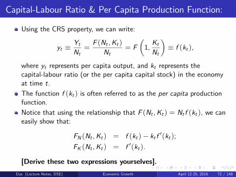
Using the CRS property, we can write:
yt ≡YtNt=F (Nt ,Kt )
Nt= F
(1,KtNt
)≡ f (kt ),
where yt represents per capita output, and kt represents thecapital-labour ratio (or the per capita capital stock) in the economyat time t.The function f (kt ) is often referred to as the per capita productionfunction.Notice that using the relationship that F (Nt ,Kt ) = Nt f (kt ), we caneasily show that:
FN (Nt ,Kt ) = f (kt )− kt f ′(kt );FK (Nt ,Kt ) = f ′(kt ).
[Derive these two expressions yourselves].
Das (Lecture Notes, DSE) Economic Growth April 12-25; 2016 72 / 148

Properties of Per Capita Production Function:
Given the properties of the aggregate production function, one canderive the following properties of the per capita production function:
(i) f (0) = 0;
(ii) f ′(k) > 0; f ′′(k) < 0;
(iii) Limk→0
f ′(k) = ∞; Limk→∞
f ′(k) = 0.
Condition (i) indicates that capital is an essential input of production;Condition (ii) indicates diminishing marginal product of capital;Condition (iii) indicates the Inada conditions with respect to capital .Finally, using the definition that kt ≡ Kt
Nt, we can write
kt+1 ≡ Kt+1Nt+1
=sF (Nt ,Kt ) + (1− δ)Kt
(1+ n)Nt
⇒ kt+1 =sf (kt ) + (1− δ)kt
(1+ n)≡ g(kt ). (14)
Das (Lecture Notes, DSE) Economic Growth April 12-25; 2016 73 / 148

Dynamics of Capital-Labour Ratio:
Equation (3) represents the basic dynamic equation in the discretetime Solow model. (Interpretation?)Notice that Equation (3) represents a single non-linear differenceequation in kt . Once again we use the phase diagram technique toanalyse the dynamic behaviour of kt .Recall that to draw the phase diagram of a single difference equation,we first plot the g(kt ) function with respect to kt . Then we identifyits possible points of intersection with the 45o line - which denote thesteady state points of the system.In plotting the g(kt ) function, note:
g(0) =sf (0) + (1− δ).0
(1+ n)= 0;
g ′(k) =1
(1+ n)
[sf ′(k) + (1− δ)
]> 0;
g ′′(k) =1
(1+ n)sf ′′(k) < 0.
Das (Lecture Notes, DSE) Economic Growth April 12-25; 2016 74 / 148
Dynamics of Capital-Labour Ratio (Contd.):
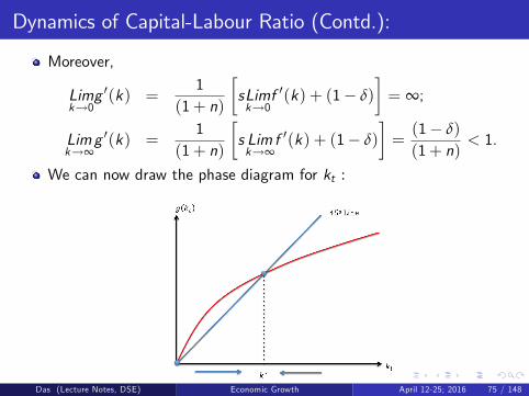
Moreover,
Limk→0
g ′(k) =1
(1+ n)
[sLimk→0
f ′(k) + (1− δ)
]= ∞;
Limk→∞
g ′(k) =1
(1+ n)
[s Limk→∞
f ′(k) + (1− δ)
]=(1− δ)
(1+ n)< 1.
We can now draw the phase diagram for kt :
Das (Lecture Notes, DSE) Economic Growth April 12-25; 2016 75 / 148
Dynamics of Capital-Labour Ratio (Contd.):
From the phase diagram we can identify two possible steady states:
(i) k = 0 (Trivial Steady State);
(ii) k = k∗ > 0 (Non-trivial Steady State).
Since an economy is always assumed to start with some positivecapital-labour ratio (however small), we shall ignore the non-trivialsteady state.The economy has a unique non-trivial steady state, given by k∗,which is globally asymptotically stable: starting from any initialcapital-labour ratio k0 > 0, the economy would always move to k∗ inthe long run.(Which assumption generates this strong stability result? Lawof diminishing returns or Inada conditions or both?)Implications:
In the long run, per capita output: yt ≡ f (kt ) will be constant atf (k∗) while aggregate output Yt ≡ Nt f (kt ) will be growing at thesame rate as Nt (namely at the exogenously given rate n).
Das (Lecture Notes, DSE) Economic Growth April 12-25; 2016 76 / 148

Some Long Run Implictions of Solow Growth Model:
Notice that the non-trivial steady state k∗ is defined as:
k∗ =sf (k∗) + (1− δ)k∗
(1+ n)⇒ (1+ n) k∗ = sf (k∗) + (1− δ)k∗
⇒ f (k∗)k∗
=n+ δ
s.
Total differentiating and using the properties of the f (k) function, itis easy to show that,
dk∗
ds> 0;
dk∗
dn< 0;
dk∗
dδ< 0.
A higher savings ratio generates a higher level of per capita output inthe long run;A higher rate of grwoth of population generates a lower level of percapita output in the long run;A higher rate of depreciation generates a lower level of per capitaoutput in the long run.[Verify these.]
Das (Lecture Notes, DSE) Economic Growth April 12-25; 2016 77 / 148

Some Long Run Implictions of Solow Growth Model(Contd.):
But these are all level effects.What would be the impact on the long run growth?Notice that among all these parameters, only a change in thepopulation growth rate (n) would have an impact upon long rungrowth.The long run growth rate in the Solovian economy is alwaysequal to n.Moreover, the economy is characterised by perpetual equalitybetween demand and supply and there is full employment ofboth the factors at every point of time.Finally, there is no role for the government in influencing the long rungrowth rate here. In particular, if the government tries to manipulatethe savings ratio (by imposing an appropriate tax on household’income and investing the tax revenue in capital formation), then sucha policy will have no long run growth effect.
Das (Lecture Notes, DSE) Economic Growth April 12-25; 2016 78 / 148

Solow Model: An Answer to Harrod?
From the above two conclusions, it appears that Solow has solvedboth the Harrodian problems:
There is no mismatch between demand and supply;There is no mismatch bewteen the growth rate of employment and thegrowth rate of population.
But recall that the first problem has simply been assumed away bySolow.
If we bring in an independent investment function in an otherwiseSolovian economy (with a Neoclassical production function), then thedemand supply mismatch is likely to reappear.
However this is an extension that has not been explored in detail inthe literature. This is food for (future) thought.
Das (Lecture Notes, DSE) Economic Growth April 12-25; 2016 79 / 148

Solow Model: Long Run vis-a-vis Short/Medium Run
In the last class we have analysed the long run growth implications ofthe Solow model.
To summarise:
The per capita income does not grow in the long run; it remainsconstatnt at f (k∗) - the exact level being determined by variousparameters (s, n, δ).The aggregate income grows at a constant rate - given by theexogenous rate of growth of population (n).
But all these happen only in the long run, i.e., as t → ∞.Starting from a given initial capital-labour ratio k0 ( 6= k∗), it willobviously take the economy some time before it reaches k∗.
What happens during these transitional periods?
In particular, what would be the rate of growth of per capita incomeand that of aggregate income in the short run - when the economy isyet to reach its steady state?
Das (Lecture Notes, DSE) Economic Growth April 12-25; 2016 80 / 148
Transitional Dynamics in Solow Growth Model:
When the economy is out of steady state, the rate of growth ofcapital-labour ratio is given by:
γk ≡kt+1 − kt
kt=
sf (kt )+(1−δ)kt(1+n) − kt
kt
=sf (kt )− (n+ δ)kt
(1+ n)ktT 0 according as kt S k∗.
Moreover,dγkdk
=−s(1+ n) [f (k)− kf ′(k)]
[(1+ n)k ]2< 0.
In other words, during transition, the higher is the capital-labour ratioof the economy, the lower is its (short run) growth rate.
This last result has important implications for cross country growthcomparisons.
Das (Lecture Notes, DSE) Economic Growth April 12-25; 2016 81 / 148

Further Implictions of Solow Growth Model: Absolutevis-a-vis Conditional Convergence
The above result implies that the transitional growth rate of percapita income in the poorer countries (with low k0) will be higherthan that of the rich countries (with high k0); and eventually they willconverge to the same level of per capita income (AbsoluteConvergence).This proposition however has been strongly rejected by data. In factempirical studies show the opposite: richers countries have remainedrich and poorer countries have remained poor and there is nosignificant tendencies towards convergence - even when one looks atlong run time series data.
The proposition of absolute convergence of course pre-supposes thatthe underlying parameters for all economies (rich and poor alike) arethe same.
Das (Lecture Notes, DSE) Economic Growth April 12-25; 2016 82 / 148
Absolute vis-a-vis Conditional Convergence (Contd.)
If we allow rich and poor countries to have different values of s, δ, netc. (which is plausible), then the Solow model generates a muchweaker prediction of Conditional Convergence.Conditional Convergence states that a country grows faster - thefurther away it is from its own steady state.
An alternative (and more useful) statement of ConditionalConvergence runs as follows: Among a group of countries which aresimilar (similar values of s, δ, n etc.), the relatively poorer ones willgrow faster and eventually the per capita income of all these countrieswill converge.
This weaker hypothesis in generally supported by data.
However, Conditional Convergence Hypothesis is not very helpful inexplaining the persistent differences in per capita income amongst therich and the poor countries.
Das (Lecture Notes, DSE) Economic Growth April 12-25; 2016 83 / 148
Solow Model: Golden Rule & Dynamic Ineffi ciency
Let us now get back from short run to long run (steady state).Recall that for given values of δ and n, the savings rate in theeconomy uniquely pins down the corresponding steady statecapital-labour ratio:
k∗(s) :f (k∗)k∗
=n+ δ
s.
We have already seen that a higher value of s is associated with ahigher k∗, and therefore, a higher level of steady state per capitaincome (f (k∗)).How about the corresponding level of consumption?Notice that in this model, per capita consumption is defined as:
CtNt
≡ Yt − StNt
⇒ ct = f (kt )− sf (kt )
Das (Lecture Notes, DSE) Economic Growth April 12-25; 2016 84 / 148

Golden Rule & Dynamic Ineffi ciency in Solow Model(Contd.)
Accordingly, for given values of δ and n, steady state level of percapita consumption is related to the savings ratio of the economy inthe following way:
c∗(s) = f (k∗(s))− sf (k∗(s))= f (k∗(s))− (n+ δ) k∗(s). [Using the definition of k∗]
We have already noted that if the government tries to manipulate thesavings ratio (by imposing an appropriate tax onconsumption/savings), then such a policy would have no long rungrowth effect.Can such a policy still generate a higher level of steady state percapita consumption at least?If yes, then such a policy would still be desirable, even if it does notimpact on growth.
Das (Lecture Notes, DSE) Economic Growth April 12-25; 2016 85 / 148

Golden Rule & Dynamic Ineffi ciency in Solow Model(Contd.)
Taking derivative of c∗(s) with respect to s :
dc∗(s)ds
=[f ′(k∗(s))− (n+ δ)
] dk∗(s)ds
.
Sincedk∗
ds> 0,
dc∗(s)ds
T 0 according as f ′(k∗(s)) T (n+ δ).
In other words, steady state value of per capita consumption, c∗(s),is maximised at that level of savings ratio and associated k∗(s) where
f ′(k∗) = (n+ δ).
We shall denote this savings ratio as sg and the corresponding steadystate capital-labour ratio as k∗g - where the subscript ‘g’stand forgolden rule.
Das (Lecture Notes, DSE) Economic Growth April 12-25; 2016 86 / 148
Digrammatic Representation of the Golden Rule SteadyState:
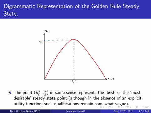
The point (k∗g , c∗g ) in some sense represents the ‘best’or the ‘most
desirable’steady state point (although in the absence of an explicitutility function, such qualifications remain somewhat vague).
Das (Lecture Notes, DSE) Economic Growth April 12-25; 2016 87 / 148

Alternative Digrammatic Representation of the GoldenRule Steady State:
There are many possible steady states to the left and to the right ofk∗g - associated with various other savings ratios.
Das (Lecture Notes, DSE) Economic Growth April 12-25; 2016 88 / 148
Golden Rule & the Concept of ‘Dynamic Ineffi ciency’
Importantly, all the steady states to the right of k∗g are called‘dynamically ineffi cient’steady states.From any such point one can ‘costlessly’move to the left - to alower steady state point - and in the process enjoy a higher level ofcurrent consumption as well as higher levels of future consumption atall subsequent dates. (How?)Notice however that the steady states to the left of k∗g are not‘dynamically ineffi cient’. (Why not?)
Das (Lecture Notes, DSE) Economic Growth April 12-25; 2016 89 / 148

Cause of ‘Dynamic Ineffi ciency’in Solow Model
Dynamic ineffi ciency occurs because people oversave.
This possibility arises in the Solow model because the savings ratiois exogenously given - it is not chosen through households’optimization process.Note that if indeed the steady state of the economy happens to lie inthe dynamically ineffi cient region, then that in itself would justify apro-active, interventionist role of the government in the Solow model- even though government cannot influence the long run rate ofgrowth of the economy.
Das (Lecture Notes, DSE) Economic Growth April 12-25; 2016 90 / 148
Limitations of the Solow Growth Model:
There are two major criticisms of the Solow model.
1 The steady state in the Solow model might be dynamically ineffi cient,because people may oversave. If one allows households to choosetheir savings ratio optimally, then this ineffi cinency should disappear.But this latter possibility is simply not allowed in the Solow model.
2 Even though the Solow model is supposed to be a growth model - itcannot really explain long run growth:
The per capita income does not grow at all in the long run;
The aggregate income grows at an exogenously given rate n, whichthe model does not attempt to explain.
Das (Lecture Notes, DSE) Economic Growth April 12-25; 2016 91 / 148
Extensions of the Solow Growth Model:
The basic Solow growth model has subsequently been extended tocounter some of these critisisms.
We shall look at two such extensions:1 Neoclassical Growth Model with Optimizing Households: Thisextension allows the households to choose their consumption/savingsbehaviour optimally over infinite horizon; developed independently byCass (1965) & Koopmans (1965).
2 Solow Model with Technological Progress: This extension allows theper capita income to grow in the long run; developed by Solow himself(Solow (1957)). In this context we shall also discuss what are thefactors that may explain this phenomenon called ‘technical progress’.
Das (Lecture Notes, DSE) Economic Growth April 12-25; 2016 92 / 148

Neoclassical Growth with Optimizing Agents:
Let us now extend the Solow model to allow for optimizing agents.
The framework which allows for optimizing consumption/savingsbehaviour by households is called:The Ramsey-Cass-Koopmans Inifinite Horizon Framework(henceforth R-C-K)This framework retains all the production side assuption of theSolovian economy; but its allows households to choose theirconsumption and savings decision optimally over an infinite horizonframework.
This latter statement should immediately tell you that the underlyingmacro structure would be very similar to the DGE framework that wehave constructed earlier.
Let us revisit the underlying macro framework.
Das (Lecture Notes, DSE) Economic Growth April 12-25; 2016 93 / 148
Neoclassical Growth with Optimizing Agents: The R-C-KModel
The R-C-K model is considered Neoclassical - because it retains allthe assumptions of the Neoclassical production function (includingthe diminishing returns property and the Inada conditions.)
In fact the production side story is exactly identical to Solow.
As before, the economy starts with a given stock of capital (Kt) anda given level of population (Lt) at time t.
These factors are supplied inelastically to the market in every period.This implies that households do not care for leisure.
Population grows at a constant rate n.
Capital stocks grows due to optimal savings (and investment)decisions by the households.
Notice that once again savings and investment are always identical.So just like Solow (and Domer), this is a supply driven growth model.
Das (Lecture Notes, DSE) Economic Growth April 12-25; 2016 94 / 148

The R-C-K Model: The Household Side Story
There are H identical households indexed by h.
Each household consists of a single infinitely lived member to beginwith (at t = 0). However population within a household increasesover time at a constant rate n. (And each newly born member isinfinitely lived too!)
At any point of time t, the total capital stock and the total labourforce in the economy are equally distributed across all the households,which they offer inelastically to the market at the market wage ratewt and the market rental rate rt .
Thus total earning of a household at time t: wtNht + rtKht .
Corresponding per member earning: yht = wt + rtkht ,where kht is the per member capital stock in household h,
which is also the per capita capital stock (or the capital-labourratio, kt) in the economy.
Das (Lecture Notes, DSE) Economic Growth April 12-25; 2016 95 / 148

The Household Side Story (Contd.):
In every time period, the instantaneous utility of the householddepends on its per member consumption:
ut = u(cht); u′ > 0; u′′ < 0; lim
ch→0u′(ch) = ∞; lim
ch→∞u′(ch) = 0.
The household at time 0 chooses its entire consumption profile{cht}∞t=0 so as to maximise the discounted sum of its life-time utility:
Uh0 =∞
∑t=0
βtu(cht)
subject to its period by period budget constraint.
Notice once again that identical households implied that permember consumption (cht ) of any household is also equal to the percapita consumption (ct) in the economy at time t.
Das (Lecture Notes, DSE) Economic Growth April 12-25; 2016 96 / 148

The R-C-K Model: Centralized Version (Optimal Growth)
There are two version of the R-C-K model:A centralized version - which analyses the problem from the perspectiveof a social planner.A decentralized version - which analyses the problem from theperspective of a perfectly competitive market economy where‘atomistic’households and firms take optimal decisions in theirrespective individual spheres.
The centralized version was developed by Ramsey (way back in 1928)and is oftem referred to as the ‘optimal growth’problem.It is assumed that there exists an omniscient, omnipotent,benevolent social planner who wants to maximise citizens’welfare.Since all households are identical, the objective function of the socialplanner is identical to that of the households:
Max .U0 =∞
∑t=0
βtu (ct ) . (15)
Das (Lecture Notes, DSE) Economic Growth April 12-25; 2016 97 / 148

The R-C-K Model: Centralized Version (Contd.)
The social planner maximises (1) subject to its period by periodbudget constraint.
Notice that in a centrally planned economy there are no markets(hence no market wage rate or market rental rate), and there is noprivate ownership of assets (capital) and no personalized income.
The social planner employs the existing capital stock in the economy(either collectively owned or owned by the government) and theexisting labour force to produce the final output -using the aggregateproduction technology.
After production it distributes a part of the total output among itscitizens for consumption puoposes and invests the rest.
Thus the budget constraint faced by the planner in period t isnothing but the aggregate resource constraint:
Ct + It = Yt = F (Kt ,Nt ).
Das (Lecture Notes, DSE) Economic Growth April 12-25; 2016 98 / 148
The R-C-K Model: Centralized Version (Contd.)
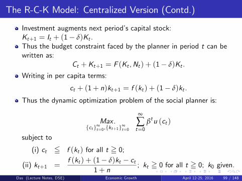
Investment augments next period’s capital stock:Kt+1 = It + (1− δ)Kt .Thus the budget constraint faced by the planner in period t can bewritten as:
Ct +Kt+1 = F (Kt ,Nt ) + (1− δ)Kt .
Writing in per capita terms:
ct + (1+ n)kt+1 = f (kt ) + (1− δ)kt .
Thus the dynamic optimization problem of the social planner is:
Max .{ct}∞
t=0,{kt+1}∞t=0
∞
∑t=0
βtu (ct )
subject to
(i) ct 5 f (kt ) for all t = 0;
(ii) kt+1 =f (kt ) + (1− δ)kt − ct
1+ n; kt = 0 for all t = 0; k0 given.
Das (Lecture Notes, DSE) Economic Growth April 12-25; 2016 99 / 148

R-C-K Model: Centralized Version (Contd.)
In Module 1, we have analysed how to solve a dynamic programmingproblem (using the Bellman equation) to arrive at the dynamicequations characterizing the optimal paths for the control and statevariable.Now we apply this technique to solve the social planner’s problem in acentralized economy.Recall that the social planner’s problem is given by:
Max .{ct}∞
t=0,{kt+1}∞t=0
∞
∑t=0
βtu (ct )
subject to
(i) ct 5 f (kt ) for all t = 0;
(ii) kt+1 =f (kt ) + (1− δ)kt − ct
1+ n; kt = 0 for all t = 0; k0 given.
Here ct is the control variable; kt is the state variable, and thecorresponding state space is given by <+.
Das (Lecture Notes, DSE) Economic Growth April 12-25; 2016 100 / 148
R-C-K Model: Centralized Version (Contd.)
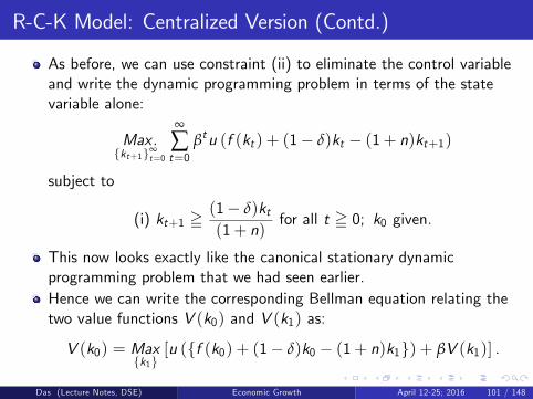
As before, we can use constraint (ii) to eliminate the control variableand write the dynamic programming problem in terms of the statevariable alone:
Max .{kt+1}∞
t=0
∞
∑t=0
βtu (f (kt ) + (1− δ)kt − (1+ n)kt+1)
subject to
(i) kt+1 =(1− δ)kt(1+ n)
for all t = 0; k0 given.
This now looks exactly like the canonical stationary dynamicprogramming problem that we had seen earlier.Hence we can write the corresponding Bellman equation relating thetwo value functions V (k0) and V (k1) as:
V (k0) = Max{k1}
[u ({f (k0) + (1− δ)k0 − (1+ n)k1}) + βV (k1)] .
Das (Lecture Notes, DSE) Economic Growth April 12-25; 2016 101 / 148
R-C-K Model: Centralized Version (Contd.)
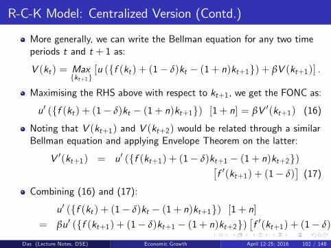
More generally, we can write the Bellman equation for any two timeperiods t and t + 1 as:
V (kt ) = Max{kt+1}
[u ({f (kt ) + (1− δ)kt − (1+ n)kt+1}) + βV (kt+1)] .
Maximising the RHS above with respect to kt+1, we get the FONC as:
u′ ({f (kt ) + (1− δ)kt − (1+ n)kt+1}) [1+ n] = βV ′(kt+1) (16)
Noting that V (kt+1) and V (kt+2) would be related through a similarBellman equation and applying Envelope Theorem on the latter:
V ′(kt+1) = u′ ({f (kt+1) + (1− δ)kt+1 − (1+ n)kt+2})[f ′(kt+1) + (1− δ)
](17)
Combining (16) and (17):
u′ ({f (kt ) + (1− δ)kt − (1+ n)kt+1}) [1+ n]= βu′ ({f (kt+1) + (1− δ)kt+1 − (1+ n)kt+2})
[f ′(kt+1) + (1− δ)
]Das (Lecture Notes, DSE) Economic Growth April 12-25; 2016 102 / 148

R-C-K Model: Centralized Version Contd.)
Now bringing back the control variable (using the constraint (ii)again), we get the FONC of the social planner’s optimization problemas:
u′ (ct ) [1+ n] = βu′ (ct+1)[f ′(kt+1) + (1− δ)
]. (18)
We also have the constraint function:
kt+1 =f (kt ) + (1− δ)kt − ct
1+ n; k0 given. (19)
Equations (18) and (19) represent a 2X2 system of differenceequations which implicitly defines the ‘optimal’trajectories of ct andkt .
Of course, we still need two boundary conditons to preciselycharacterise the solution paths for this 2X2 system.
Das (Lecture Notes, DSE) Economic Growth April 12-25; 2016 103 / 148
R-C-K Model: Centralized Version (Contd.)
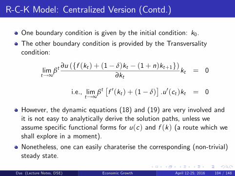
One boundary condition is given by the initial condition: k0.
The other boundary condition is provided by the Transversalitycondition:
limt→∞
βt∂u ({f (kt ) + (1− δ)kt − (1+ n)kt+1})
∂ktkt = 0
i.e., limt→∞
βt[f ′(kt ) + (1− δ)
].u′(ct )kt = 0
However, the dynamic equations (18) and (19) are very involved andit is not easy to analytically derive the solution paths, unless weassume specific functional forms for u(c) and f (k) (a route which weshall explore in a moment).
Nonetheless, one can easily charaterise the corresponding (non-trivial)steady state.
Das (Lecture Notes, DSE) Economic Growth April 12-25; 2016 104 / 148
R-C-K Model (Centralized Version): Steady State
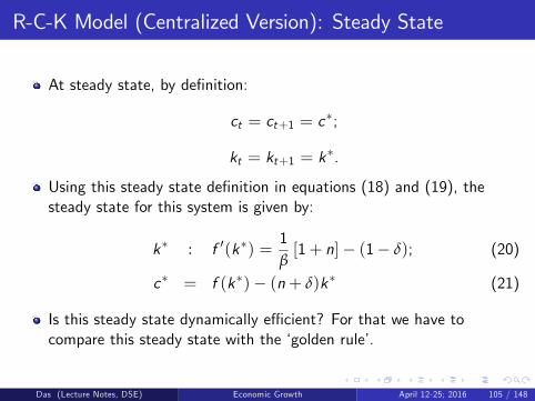
At steady state, by definition:
ct = ct+1 = c∗;
kt = kt+1 = k∗.
Using this steady state definition in equations (18) and (19), thesteady state for this system is given by:
k∗ : f ′(k∗) =1β[1+ n]− (1− δ); (20)
c∗ = f (k∗)− (n+ δ)k∗ (21)
Is this steady state dynamically effi cient? For that we have tocompare this steady state with the ‘golden rule’.
Das (Lecture Notes, DSE) Economic Growth April 12-25; 2016 105 / 148
R-C-K Model (Centralized Version): Golden Rule &Dynamic Effi ciency
Recall that in the Solow model, the ‘golden rule’defines a particularsavings ratio (sg ) and the corresponding k∗g such that the per capitaconsumption (at steady state) is maximised. This was given by:
k∗g : f ′(k∗g ) = (n+ δ)
Is the above definition of ‘golden rule’still valid for this R-C-K model?
Note that the savings ratio is the R-C-K model is endogenous. So wecannot compare between various steady states arising out of varioussavings ratio.
Indeed, optimal savings bahaviour in the R-C-K throws up a uniquesteady state (k∗, c∗), as defined by equations (20) and (21) above.
Das (Lecture Notes, DSE) Economic Growth April 12-25; 2016 106 / 148
R-C-K Model (Centralized Version): Golden Rule &Dynamic Effi ciency (Contd.)
However, we can still compare it with various quasi-steady statepoints which are defined as follows:
Consider various (k, c) combinations in the economy such that if youare at one of these (k, c) points then you can maintain that forever(although it may not be optimal).Any particular k can be maintained forever if and only if the per capitasavings/investment is just enough to accomodate the new membersthat are to be born in the next period as well as to compensate for thedepreciated capital stock.In other words, any capital stock k can be maintained forever ever iff (k)− c = (n+ δ)k.This immediately tells us that for any k, there exists a particular c ,given by c = f (k)− (n+ δ)k , such that this (k, c) combination canbe maintained forever.Clearly, the steady state of the R-C-K model, (k∗, c∗), represents onesuch quasi-steady state (as is obvious from equation 21).
Das (Lecture Notes, DSE) Economic Growth April 12-25; 2016 107 / 148

R-C-K Model (Centralized Version): Golden Rule &Dynamic Effi ciency (Contd.)
The next question is: amongst all these quasi-steady state points,which one is associated with the highest value of per capitaconsumption (that can be sustained for ever)?Turns out that the quasi-steady state point with highest level ofconsumption is none other than the golden rule point:
k∗g : f ′(k∗g ) = (n+ δ)
Indeed, just as we had argued before, any quasi-steady state pointthat lies to the right of the golden rule is dynamically ineffi cientbecause from there one can costlessly move to the golden rule pointand enjoy higher consumption level today and in future.But the quasi-steady state points lying to the left of the golden ruleare all effi cient point, because to move from there to the golden rule,one has to save some extra units - which implies some currentconsumption foregone. Hence such a move is not costless.
Das (Lecture Notes, DSE) Economic Growth April 12-25; 2016 108 / 148

R-C-K Model (Centralized Version): Golden Rule &Dynamic Effi ciency (Contd.)
The steady state of the R-C-K model, (k∗, c∗), indeed lies in thedynamically effi cient region. (Proof?)In fact, when β = 1, then steady state of the R-C-K model, (k∗, c∗),(which is part of the optimal trajectory for the economy) coincideswith the golden rule point.
Thus we see that in the centralized version of the R-C-K model, whenthe social planner decides on how much to save and how much toleave for households’consumption in order to maximise households’utility over infinite horizon, it ensures that the corresponding steadystate is not dynamically ineffi cient.But this is a result that is to be expected from an omnipotent andomniscient central planner.
Will this result hold for a decentralized market economy as well?We’ll see.
Das (Lecture Notes, DSE) Economic Growth April 12-25; 2016 109 / 148
R-C-K Model (Centralized Version): Optimal Paths
Before we move to the decentralized version of the R-C-K model, letus characterise the precise optimal paths of consumption and capitalstock for this centralized economy.
For analytical convenience, we shall use specific functional forms foru(c) and f (k).
Letu(ct ) = log ct ;
f (kt ) = (kt )α ; 0 < α < 1.
Also let the rate of depreciation be 100%, i.e., δ = 1.
Das (Lecture Notes, DSE) Economic Growth April 12-25; 2016 110 / 148

R-C-K Model (Centralized Version): Optimal Paths(Contd.)
Given these specific functional forms, the dynamic equations for thecentralized R-C-K model are represented by the following twoequations:
ct+1ct
= β
[α(kt+1)α−1]1+ n
; (22)
kt+1 =(kt )α − ct1+ n
. (23)
The associated boundary conditions are:
k0 given; limt→∞
βtα(kt )α−1.ktct= 0
Das (Lecture Notes, DSE) Economic Growth April 12-25; 2016 111 / 148
Characterization of the Optimal Paths:
We are now all set to characterise the dynamic paths of ct and kt ascharted out by the above dynamic system.Before that let us quickly characterize the steady state.Using the steady state condition that ct = ct+1 = c∗ andkt = kt+1 = k∗ in equations (22) and (23), the steady state valuesare given by:
k∗ =
(αβ
1+ n
) 11−α
;
c∗ = (k∗)α − (1+ n)k∗.Now let us chart out the optimal paths of ct and kt - starting fromany given initial value of k0. (Note that the initial value of c0 is notgiven - it is to be optimally determined).We could have used the phase diagram method to qualitativelycharacterise the solution paths. But instead, we shall use the directmethod of ‘guess and verify’.
Das (Lecture Notes, DSE) Economic Growth April 12-25; 2016 112 / 148
Characterization of the Optimal Paths (Contd.):
Under the ‘guess and verify’method, we first make an arbitrary guessabout how the solution would look. Since any solution must satisfythe given dynamic equations, we then try to verify if our proposedconjecture can indeed be a solution or not.Let us now make a conjecture that the optimal path of per capitastock looks as follows:
kt+1 = M (kt )α for all t, (C)
where M is a yet unknown constant.If (C) is indeed the solution path for kt+1 for all t, then (from (23))the corresponding solution path for ct would be given by:
ct = (kt )α − (1+ n)kt+1 = [1−M(1+ n)] (kt )α.
Likewise,ct+1 = [1−M(1+ n)] (kt+1)α.
Das (Lecture Notes, DSE) Economic Growth April 12-25; 2016 113 / 148

Characterization of the Optimal Paths (Contd.):
Now these conjectured solutions for ct and ct+1 must satisfy equation(22).Plugging these values in (22):
[1−M(1+ n)] (kt+1)α
[1−M(1+ n)] (kt+1)α= β
[α(kt+1)α−1]1+ n
i.e.,(kt+1)α
(kt )α=
αβ(kt+1)α−1
1+ n
i.e., kt+1 =αβ
1+ n(kt )α
Recall that our conjecture was: kt+1 = M(kt )α.Hence our conjecture would indeed be true (and satisfy all therelevant equations) if and only if
M ≡ αβ
1+ n.
Das (Lecture Notes, DSE) Economic Growth April 12-25; 2016 114 / 148
Characterization of the Optimal Paths (Contd.):
Thus by the guess and verify method we have indeed identifed theoptimal solution paths of ct and kt for this dynamic problem.
These optimal paths are:
ct = (1− αβ) (kt )α for all t = 0;
kt+1 =αβ
1+ n(kt )α for all t = 0.
It is easy to check that starting from any k0, the ct and kt valuesmonotonically approach their respective steady state values c∗ and k∗.
So the strong stability result of Solow is preserved, and the steadystate is now necessarily dynamically effi cient.Growth predictions are exactly the same as that of the Solow model:
The per capita income does not grow in the long run;The aggregate income in the long run grows at a constant exogenousrate n.
Das (Lecture Notes, DSE) Economic Growth April 12-25; 2016 115 / 148
R-C-K Model: the De-centralized Version
We have just analysed the centralized version of the R-C-K model,where a benevolent social planner makes all the production andsavings/investment decisions on behalf of the households.
We now turn to the corresponding problem for a decentralized marketeconomy, where all these economic decisions are undertaken by‘atomistic’firms and households.
Perfect competition prevails - which means that while optimizing, thefirms and households take all the market prices (in the commoditymarket as well as in the factor markets) as given.
The decentralized market economy under the R-C-K model is exactlyanalogous to the general equilibrium set up of the DGE modelwithout adjustment costs.
Since we had derived the dynamic equations for the latter case indetail, let us quickly revisit the set up.
Das (Lecture Notes, DSE) Economic Growth April 12-25; 2016 116 / 148

R-C-K Model (De-centralized Version): Production SideStory
Recall that the production side story is identical to that of Solow.
Thus all firms have access to an identical production technology -which satisfies all standard neoclassical properties.
The firm-specific production functions can be aggregated to generatean aggregate production function such that :
Yt = F (Kt ,Nt ).
At every point of time the market clearing wage rate and the rentalrate of capital are given by:
wt = FN (Kt ,Nt ); rt = FK (Kt ,Nt ).
At these wage rate and rental rate, there is full employment of boththe factors.
Das (Lecture Notes, DSE) Economic Growth April 12-25; 2016 117 / 148

R-C-K Model (De-centralized Version): Household SideStory
In the absence of intra-household borrowing, the representativehousehold h’s problem would given by:
Max .{cht }∞
t=0,{kht+1}∞
t=0
∞
∑t=0
βtu(cht)
subject to
(i) cht 5 wt + rtkht for all t = 0;
(ii) kht+1 =wt + rtkht + (1− δ)kht − cht
1+ n; kht = 0 for all t = 0; kh0 given.
where cht is the control variable; kht is the state variable, and the
corresponding state space is given by <+.
Das (Lecture Notes, DSE) Economic Growth April 12-25; 2016 118 / 148
De-centralized R-C-K Model: Household Side Story(Contd.)
Notice that in order to solve this problem the households would haveto have some expectation about the entire future time paths of wtand rt .
We shall however assume that the households’are endowed withperfect foresight, which enables them to correctly guess all thefuture values of the market wage rate and rental rate.
Let us also assume that households can potentially borrow from eachother (although with identical households this option would never beexercised).
Allowing for intra-household borrowings of course means that we shallhave to consider two forms of assets:
1 physical capital (Kht );2 financial capital, i.e., lending to other households (Lht ≡ −Bht ).
Das (Lecture Notes, DSE) Economic Growth April 12-25; 2016 119 / 148
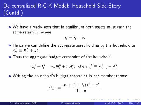
De-centralized R-C-K Model: Household Side Story(Contd.)
We have already seen that in equlibrium both assets must earn thesame return rt , where
rt = rt − δ.
Hence we can define the aggregate asset holding by the household asAht ≡ K ht + Lht .Thus the aggregate budget constraint of the household:
C ht + Iht = wtN
ht + rtA
ht , where I
ht ≡ Aht+1 − Aht .
Writing the household’s budget constraint in per member terms:
aht+1 =wt + (1+ rt )aht − cht
1+ n.
Das (Lecture Notes, DSE) Economic Growth April 12-25; 2016 120 / 148
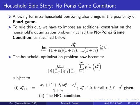
Household Side Story: No Ponzi Game Condition:
Allowing for intra-household borrowing also brings in the possibility ofPonzi game.To rule this out, we have to impose an additional constraint on thehousehold’s optimization problem - called the No-Ponzi GameCondition, as specified below:
limt→∞
Aht(1+ r0)(1+ r1)......(1+ rt )
= 0.
The household’optimization problem now becomes:
Max .{cht }∞
t=0,{kht+1}∞
t=0
∞
∑t=0
βtu(cht)
subject to
(i) aht+1 =wt + (1+ rt )aht − cht
1+ n; aht ∈ < for all t = 0; ah0 given.
(ii) The NPG condition.
Das (Lecture Notes, DSE) Economic Growth April 12-25; 2016 121 / 148
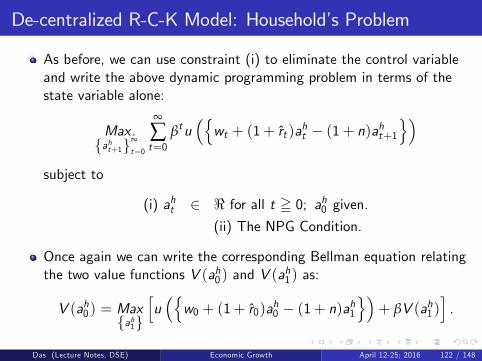
De-centralized R-C-K Model: Household’s Problem
As before, we can use constraint (i) to eliminate the control variableand write the above dynamic programming problem in terms of thestate variable alone:
Max .{aht+1}∞
t=0
∞
∑t=0
βtu({wt + (1+ rt )aht − (1+ n)aht+1
})subject to
(i) aht ∈ < for all t = 0; ah0 given.(ii) The NPG Condition.
Once again we can write the corresponding Bellman equation relatingthe two value functions V (ah0) and V (a
h1) as:
V (ah0) = Max{ah1}
[u({w0 + (1+ r0)ah0 − (1+ n)ah1
})+ βV (ah1)
].
Das (Lecture Notes, DSE) Economic Growth April 12-25; 2016 122 / 148

Household’s Problem: Bellman Equation
More generally, we can write the Bellman equation for any two timeperiods t and t + 1 as:
V (aht ) = Max{aht+1}
[u({wt + (1+ rt )aht − (1+ n)aht+1
})+ βV (aht+1)
].
Maximising the RHS above with respect to aht+1, from the FONC:
u′({wt + (1+ rt )aht − (1+ n)aht+1
})[1+ n] = βV ′(aht+1) (24)
Noting that V (aht+1) and V (aht+2) would be related through a similar
Bellman equation and applying Envelope Theorem on the latter:
V ′(aht+1) = u′({wt+1 + rt+1aht+1 − (1+ n)aht+2
}).(1+ rt+1).
(25)
Das (Lecture Notes, DSE) Economic Growth April 12-25; 2016 123 / 148

Household’s Problem: Optimal Solutions
Combining (24) and (25) and noting that the terms inside the u′(.)functions are nothing but cht and c
ht+1 respectively, we get the FONC
of the household’s optimization problem as:
u′(cht)[1+ n] = βu′
(cht+1
)(1+ rt+1). (26)
We also have the constraint function:
aht+1 =wt + (1+ rt )aht − cht
1+ n; ah0 given. (27)
Equations (26) and (27) represents a 2X2 system of differenceequations which implicitly defines the ‘optimal’trajectories
{cht}∞t=0
and{aht+1
}∞t=0.
The two boundary conditons are given by the initial condition ah0 , andthe NPG condition.
Das (Lecture Notes, DSE) Economic Growth April 12-25; 2016 124 / 148
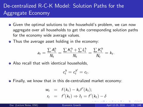
De-centralized R-C-K Model: Solution Paths for theAggregate Economy
Given the optimal solutions to the household’s problem, we can nowaggregate over all households to get the corresponding solution pathsfor the economy wide average values.Thus the average asset holding in the economy:
at =∑AhtNt
=∑K ht +∑ Lht
Nt=
∑K htNt
= kt .
Also recall that with identical households,
cht = ch′t = ct .
Finally, we know that in this de-centralized market economy:
wt = f (kt )− kt f ′(kt );rt = f ′(kt )⇒ rt = f ′(kt )− δ
Das (Lecture Notes, DSE) Economic Growth April 12-25; 2016 125 / 148
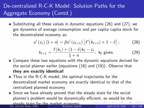
De-centralized R-C-K Model: Solution Paths for theAggregate Economy (Contd.)
Substituting all these values in dynamic equations (26) and (27), weget dynamics of average consumption and per capita capita stock forthe decentralized economy as:
u′ (ct ) [1+ n] = βu′ (ct+1)[f ′(kt+1) + 1− δ
]; (28)
kt+1 =f (kt ) + (1− δ)kt − ct
1+ n; k0 given. (29)
Compare these two equations with the dynamic equations derived forthe social planner earlier (equations (18) and (19)). Observe thatthey are exactly identical!Thus in the R-C-K model, the optimal trajectories for thedecentralized market economy are exactly identical to that of thecentralized planned economy.Since we have already proved that the steady state for the socialplanner’s problem would be dynamically effi cient, so would be thesteady state for the market economy.
Das (Lecture Notes, DSE) Economic Growth April 12-25; 2016 126 / 148

Equivalence between a Planned Economy & the MarketEconomy under R-C-K Model: Implications
The equivalence of outcomes between the socially planned economyand the competitive market economy is a very strong result.It implies that the optimizing behaviour of ‘atomistic’agents, actingin their individual spheres, would result in an outcome which isexactly identical to that of the omniscient, omnipotent social planner(or governement).Thus there is no logical scope for government intervention here -either in terms of influencing the long run growth rate (which itcannot affect anyway) or in terms of improving effi ciency (which issuperfluous, because now the market economy is already effi cient)!Note however that this strong equivalence result depends crucially onthe assumption that households have perfect foresight/rationalexpectations. Without this assumption, the equivalence resultbreaks down; the optimal trajectory chosen by the market economywill no longer be socially optimal.
Das (Lecture Notes, DSE) Economic Growth April 12-25; 2016 127 / 148
Long Run Growth of Per Capita Income: TechnologicalProgress
As we have noted before, the standard neoclassical growth model(either Solow or R-C-K) cannot explain long run growth of per capitaincome.
Since the capital-labour ratio goes to a constant in the long run, sodoes per capita output.
It is diffi cult to reconcile this result with empirical observations. If onelooks at the world economy as a whole over the last two centuries,there has been tremedous improvement in the average standard ofliving in all countries.Not being able to explain this growth pattern is a major shortcomingof the Solow growth model.
Solow himself was aware of this shortcoming. To address this, in asubsequest paper he introduced ‘technological progress’.
Das (Lecture Notes, DSE) Economic Growth April 12-25; 2016 128 / 148

What is Technological Progress?
Let us now introduce a productivity-related term into our firm-specificproduction function:
Yit = F (Kit ,Nit ,At );FA > 0,
where F satisfies all the standard Neoclassical properties specifiedearlier.The term At captures the state of the technology at time t. Since allfirms have access to identical technology, this technology-specificparameter is the same for all firms (hence no i-subscript here).The assumption of identical firms and CRS implies that the aggregateproduction function will also take similar form:
Yt = F (Kt ,Nt ,At );FA > 0.
Technological progress implies that the productivity-specific term, At ,increases in value over time. Thus with the same amount of labourand capital, the economy can now produce greater amount of output.
Das (Lecture Notes, DSE) Economic Growth April 12-25; 2016 129 / 148

Different Types of Technological Progress:
Technological progress can be of three types:1 Labour Augmenting or Harrod-Neutral: Technical improvementenhances the productivity of labour alone:
Yt = F (Kt ,AtNt ).
2 Capital Augmenting or Solow-Neutral: Technical improvementenhances the productivity of capital alone:
Yt = F (AtKt ,Nt ).
3 Capital & Labour Augmenting or Hicks-Neutral: Technicalimprovement enhances the productivity of both capital and labour inequal proportion and thus augments total factor productivity:
Yt = F (AtKt ,AtNt ) = AtF (Kt ,Nt ).
Das (Lecture Notes, DSE) Economic Growth April 12-25; 2016 130 / 148

Technological Progress and Balanced Growth:
Modern growth theory often focuses on Balanced Growth Path: ascenario when every variable in the economy grows at some constantrate.
Recall that steady state is also a special case of balanced growth(when the growth rate is constant at 0).
It can be shown that only Harrod-neutral technological progress isconsistent with balanced growth path.
In what follows, we shall therefore restrict our analysis only toHarrod-neutral technological progress.
Notice however that for Cobb-Douglas production function, all thethree notions of technical progress are equivalent. (Prove this.)
Das (Lecture Notes, DSE) Economic Growth April 12-25; 2016 131 / 148
Solow Model with Harrod-Neutral Technological Progress:
Suppose all assumptions of the original Solow model remainunchanged, except that we have now added a technology index At inthe firm-specific production technology:
Yit = F (Kit ,AtNit ).
The corresponding aggregate production technology is given by
Yt = F (Kt ,AtNt ) ≡ F (Kt , Nt ),where we denote the productivity-augmented labour term: AtNt ≡ Nt(effective labour).Labour productivity increases automatically over time (like ‘mannafrom heaven’) at an exogenous rate m:
At+1 = (1+m)At .
Each firm now equates the marginal product of ‘effective labour’withthe wage rate per unit of ‘effective labour’(w) and the marginalproduct of capital with the rental rate of capital (r).
Das (Lecture Notes, DSE) Economic Growth April 12-25; 2016 132 / 148
Solow Model with Harrod-Neutral Technological Progress(Contd.):
CRS and identical firms implies that the firm-specific marginalproduct and the (social) marginal product for the aggregate economyare the same.
Thus we get the aggregate demand functions for ‘effective labour’and capital as:
FN (Kit , Nit ) = FN (Kt , Nt ) = wt ;
FK (Kit , Nit ) = FK (Kt , Nt ) = rt .
At the beginning of any time period t, the economy starts with agiven stock of population (Nt), a given stock of capital (Kt) and agiven level of labour productivity (At).
The wage rate and rental rate adjust so that that there is fullemployment of all the factors at every point of time t.
Das (Lecture Notes, DSE) Economic Growth April 12-25; 2016 133 / 148

Capital- Effective Labour Ratio & Output per unit ofEffective Labour:
As before, Uusing the CRS property, we can write:
yt ≡YtNt=F (Kt ,AtNt )
AtNt= F
(KtAtNt
, 1)≡ f (kt ),
where yt represents output per unit of effective labour, and ktrepresents the capital-effective labour ratio in the economy at time t.
Using the relationship that F (Kt , Nt ) = Nt f (kt ), we can easily showthat:
FN (Nt ,Kt ) = f (kt )− kt f ′(kt ) = wt ;FK (Nt ,Kt ) = f ′(kt ) = rt .
[Derive these two expressions yourselves].
Das (Lecture Notes, DSE) Economic Growth April 12-25; 2016 134 / 148

Properties of the Reduced Form Production Function:
Once again, given the properties of the aggregate productionfunction, one can derive the following properties of the reduced formproduction function (in terms of effective labour) f (k):
(i) f (0) = 0;
(ii) f ′(k) > 0; f ′′(k) < 0;
(iii) Limk→0
f ′(k) = ∞; Limk→∞
f ′(k) = 0.
Finally, using the definition that kt ≡ KtAtNt
, we can write
kt+1 ≡ Kt+1At+1Nt+1
=sF (Kt ,AtNt ) + (1− δ)Kt(1+m)At (1+ n)Nt
⇒ kt+1 =sf (kt ) + (1− δ)kt(1+m)(1+ n)
≡ g(kt ). (30)
Das (Lecture Notes, DSE) Economic Growth April 12-25; 2016 135 / 148
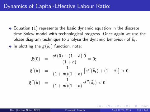
Dynamics of Capital-Effective Labour Ratio:
Equation (1) represents the basic dynamic equation in the discretetime Solow model with technological progress. Once again we use thephase diagram technique to analyse the dynamic behaviour of kt .
In plotting the g(kt ) function, note:
g(0) =sf (0) + (1− δ).0
(1+ n)= 0;
g ′(k) =1
(1+m)(1+ n)
[sf ′(kt ) + (1− δ)
]> 0;
g ′′(k) =1
(1+m)(1+ n)sf ′′(kt ) < 0.
Das (Lecture Notes, DSE) Economic Growth April 12-25; 2016 136 / 148
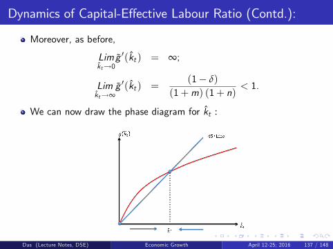
Dynamics of Capital-Effective Labour Ratio (Contd.):
Moreover, as before,
Limkt→0
g ′(kt ) = ∞;
Limkt→∞
g ′(kt ) =(1− δ)
(1+m) (1+ n)< 1.
We can now draw the phase diagram for kt :
Das (Lecture Notes, DSE) Economic Growth April 12-25; 2016 137 / 148

Dynamics of Capital-Effective Labour Ratio (Contd.):
From the phase diagram we can identify two possible steady states:
(i) k = 0 (Trivial Steady State);
(ii) k = k∗ > 0 (Non-trivial Steady State).
As before, ignoring the non-trivial steady state, we get a uniquenon-trivial steady state, k∗, which is globally asymptotically stable:starting from any initial capital-effective labour ratio k0 > 0, theeconomy would always move to k∗ in the long run.
Implication:
In the long run, output per unit of effective labour: yt ≡ f (kt ) will beconstant at f (k∗).
Das (Lecture Notes, DSE) Economic Growth April 12-25; 2016 138 / 148

Long Run Growth Implications of Solow Model withTechnological Progress:
What about per capita income?
Notice that now per capita income grows at a constant rate m in thelong run.Correspondingly, aggregate income grows at a constant rate (m+ n).
Thus incorporating technical progress in the Solow model indeedallows us to counter the critisism that per capita income does notgrow in the long run.
Notice however that both the long run growth rates are stillexogenous; we still do not know what determines m and n.
Thus the Solow model still does not tell us what determineslong run economic growth!!
Das (Lecture Notes, DSE) Economic Growth April 12-25; 2016 139 / 148

Long Run Growth of Per Capita Income withoutTechnological Progress?
Exogenous technological progress is not a very satisfactory way toexplain long run growth of per capita income.
Without a proper theory to explain this phenomenon, it remains amere technical exercise.
Can we have long run growth of per capita income in a Solovianeconomy - even without technical progress?
The answer is: yes, but only if you allow some of the Neoclassicalproperties of the production function to be relaxed.
Recall that the long run constancy of the per capita income in theSolow model arises due to the strong uniqueness and stability propertyof the steady state - which in turn depends on two key assumptions:the property of diminishing returns and the Inada Conditions.
The simplest way to generate long run growth of per capita income inthe Solow model is to allow for relaxation of one of these conditions.
Das (Lecture Notes, DSE) Economic Growth April 12-25; 2016 140 / 148

AK Production Technology: First Step TowardsEndogenous Growth?
In particular, steady growth along a balanced growth path is possibleif the production function exhibits non-diminishing returns.A specific example of such non-diminishing returns technology is theAK technology where output is a linear function of capital:
Yt = AKt .
The AK model is the precursor to the latter-day ‘endogenous growththeory’which (unlike Solow) attempts to explain technologicalprogress in terms endogenous factors within the economy.
When technology interacts with the factor accumulation, there is noreason why the production function would necessarily exhibitdiminishing returns.
Das (Lecture Notes, DSE) Economic Growth April 12-25; 2016 141 / 148
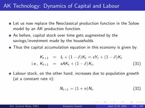
AK Technology: Dynamics of Capital and Labour
Let us now replace the Neoclassical production function in the Solowmodel by an AK production function.
As before, capital stock over time gets augmented by thesavings/investment made by the households.
Thus the capital accumulation equation in this economy is given by:
Kt+1 = It + (1− δ)Kt = sYt + (1− δ)Kti.e., Kt+1 = sAKt + (1− δ)Kt , (31)
Labour stock, on the other hand, increases due to population growth(at a constant rate n):
Nt+1 = (1+ n)Nt . (32)
Das (Lecture Notes, DSE) Economic Growth April 12-25; 2016 142 / 148

AK Technogy: Dynamics of Capital-Labour Ratio
Using the definition that kt ≡ KtNt, we can write
kt+1 ≡ Kt+1Nt+1
=sAKt + (1− δ)Kt
(1+ n)Nt
⇒ kt+1 =sA+ (1− δ)
(1+ n)kt . (33)
From above, the rate of growth of capital-labour ratio, and hencethat of per capita output, is immediately given by:
kt+1 − ktkt
=sA− (δ+ n)(1+ n)
As long as sA > (δ+ n), per capita output grows at a constant rate -both in short run and long run.
Das (Lecture Notes, DSE) Economic Growth April 12-25; 2016 143 / 148

Justifications for AK Technology:
There are many justifications as to why the ‘aggregate’productiontechnology might be linear. Here we look at two examples - eachproviding a different justification as to why diminishing returns mightnot work:
1 Fixed Coeffi cient Technogy - exhibiting complemetarity between factorsof production;
2 Production Technology with Learning-by-Doing and KnowledgeSpillover (Frankel-Romer).
Das (Lecture Notes, DSE) Economic Growth April 12-25; 2016 144 / 148
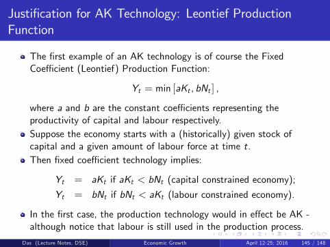
Justification for AK Technology: Leontief ProductionFunction
The first example of an AK technology is of course the FixedCoeffi cient (Leontief) Production Function:
Yt = min [aKt , bNt ] ,
where a and b are the constant coeffi cients representing theproductivity of capital and labour respectively.Suppose the economy starts with a (historically) given stock ofcapital and a given amount of labour force at time t.Then fixed coeffi cient technology implies:
Yt = aKt if aKt < bNt (capital constrained economy);
Yt = bNt if bNt < aKt (labour constrained economy).
In the first case, the production technology would in effect be AK -although notice that labour is still used in the production process.
Das (Lecture Notes, DSE) Economic Growth April 12-25; 2016 145 / 148

Justification for AK Technology: Learning by Doing &Knowledge Spillover
A more nuanced justification was provided by Frankel (1962), whichwas later exploited by Romer (1986) in developing the first model ofendogenous growth.Consider an economy with S identical firms - each having access toan identical firm-specific technology:
Yi = AtF (Kit ,Nit ) ≡ At (Kit )α (Nit )1−α ; 0 < α < 1.
Note that the firm-specific production function exhibits all theneoclassical properties.The term At represents the current state of the technology in theeconomy, which is treated as exogenous by each firm.Frankel relates the At term to the aggregate capital labour-ratio inthe economy - due to ‘learning by doing’:
At = g(KtNt
); g ′ > 0; where Kt = SKit ; N = SNit .
Das (Lecture Notes, DSE) Economic Growth April 12-25; 2016 146 / 148
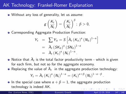
AK Technology: Frankel-Romer Explanation
Without any loss of generality, let us assume:
g(KtNt
)=
(KtNt
)β
; β > 0,
Corresponding Aggregate Production Function:
Yt = ∑Yit = S[At (Kit )
α (Nit )1−α]
= At (SKit )α (SNit )
1−α
= At (Kt )α (Nt )
1−α .
Notice that At is the total factor productivity term - which is givenfor each firm, but not so for the aggregate economy.Replacing the value of At in the aggregate production technology:
Yt = At (Kt )α (Nt )
1−α = (Kt )α+β (Nt )
1−α−β .
In the special case where α+ β = 1, the aggregate productiontechnology is indeed AK.
Das (Lecture Notes, DSE) Economic Growth April 12-25; 2016 147 / 148
AK Technology: General Insight
Even though the AK models hint at some explanation for thetechnology parameter (e.g., learning by doing in the Frankel-Romermodel), they do not model technological progress explicitly.
The subsequent endogenous growth models explicitly specify aprocess of technological change in terms of R&D, education,improvement in infrastructure etc. They also move away from theCRS technology to allow for IRS - which necessitates a movementaway from competitive market structure.
Even more recent developments in growth theory go beyondtechnology and explain growth in terms of other deeper factors likeinstitutions, political economy, income and wealth distribution etc.
These are however beyond the purview of the current course.
Das (Lecture Notes, DSE) Economic Growth April 12-25; 2016 148 / 148