Outline Training Examples for EnjoySport learning and... · Sunny Warm High Strong Warm Same Yes ... Example Version Space Sky Temp Humid Wind Water Forecst EnjoySpt ... Three Learners

Outline

[read Chapter 2][suggested exercises 2.2, 2.3, 2.4, 2.6]

• Learning from examples

• General-to-specific ordering over hypotheses

• Version spaces and candidate elimination algorithm

• Picking new examples

• The need for inductive bias

Note: simple approach assuming no noise, illustrates key concepts

1 lecture slides for textbook Machine Learning, c⃝Tom M. Mitchell, McGraw Hill, 1997

Training Examples for EnjoySport

Sky Temp Humid Wind Water Forecst EnjoySptSunny Warm Normal Strong Warm Same YesSunny Warm High Strong Warm Same YesRainy Cold High Strong Warm Change NoSunny Warm High Strong Cool Change Yes

What is the general concept?


Representing Hypotheses


Many possible representations

Here, h is conjunction of constraints on attributes

Each constraint can be

• a specfic value (e.g., Water = Warm)

• don’t care (e.g., “Water =?”)

• no value allowed (e.g.,“Water=∅”)

For example,Sky AirTemp Humid Wind Water Forecst⟨Sunny ? ? Strong ? Same⟩

Classify everything negative⟨φ,φ,φ,φ,φ,φ⟩

Classify everything positive⟨?, ?, ?, ?, ?, ?⟩


Prototypical Concept Learning Task


• Given:

– Instances X : Possible days, each described by the attributes Sky, AirTemp, Humidity, Wind,Water, Forecast

– Target function c: EnjoySport : X → {0, 1}– Hypotheses H : Conjunctions of literals. E.g.

⟨?, Cold,High, ?, ?, ?⟩.

– Training examples D: Positive and negative examples of the target function

⟨x1, c(x1)⟩, . . . ⟨xm, c(xm)⟩

• Determine: A hypothesis h in H such that h(x) = c(x) for all x in D.


The inductive learning hypothesis: Any hypothesis found to approximate the target function wellover a sufficiently large set of training examples will also approximate the target function well overother unobserved examples.


Instance, Hypotheses, and More-General-Than


h = <Sunny, ?, ?, Strong, ?, ?>h = <Sunny, ?, ?, ?, ?, ?>h = <Sunny, ?, ?, ?, Cool, ?>

2h

h 3h

Instances X Hypotheses H

Specific

General

1x

2x

x = <Sunny, Warm, High, Strong, Cool, Same>x = <Sunny, Warm, High, Light, Warm, Same>

1

1

2

1

23


Find-S Algorithm

1. Initialize h to the most specific hypothesis in H

2. For each positive training instance x

• For each attribute constraint ai in h

If the constraint ai in h is satisfied by x

Then do nothing

Else replace ai in h by the next more general constraint that is satisfied by x

3. Output hypothesis h


Hypothesis Space Search by Find-S


Instances X Hypotheses H

Specific

General

1x2x

x 3

x4

h0h1

h2,3

h4

+ +

+

x = <Sunny Warm High Strong Cool Change>, +4

x = <Sunny Warm Normal Strong Warm Same>, +1x = <Sunny Warm High Strong Warm Same>, +2x = <Rainy Cold High Strong Warm Change>, -3

h = <Sunny Warm Normal Strong Warm Same>1h = <Sunny Warm ? Strong Warm Same>2

h = <Sunny Warm ? Strong ? ? >4

h = <Sunny Warm ? Strong Warm Same>3

0h = <∅, ∅, ∅, ∅, ∅, ∅>

-

Generalisation only as far as necessary!

IF hypothesis is conjuction of attribute constraints

THEN guarantees most specific hypothesis in H that is consistent with the positive examples

also consistent with the negative examples provided target concept ∈ H, training examples correct


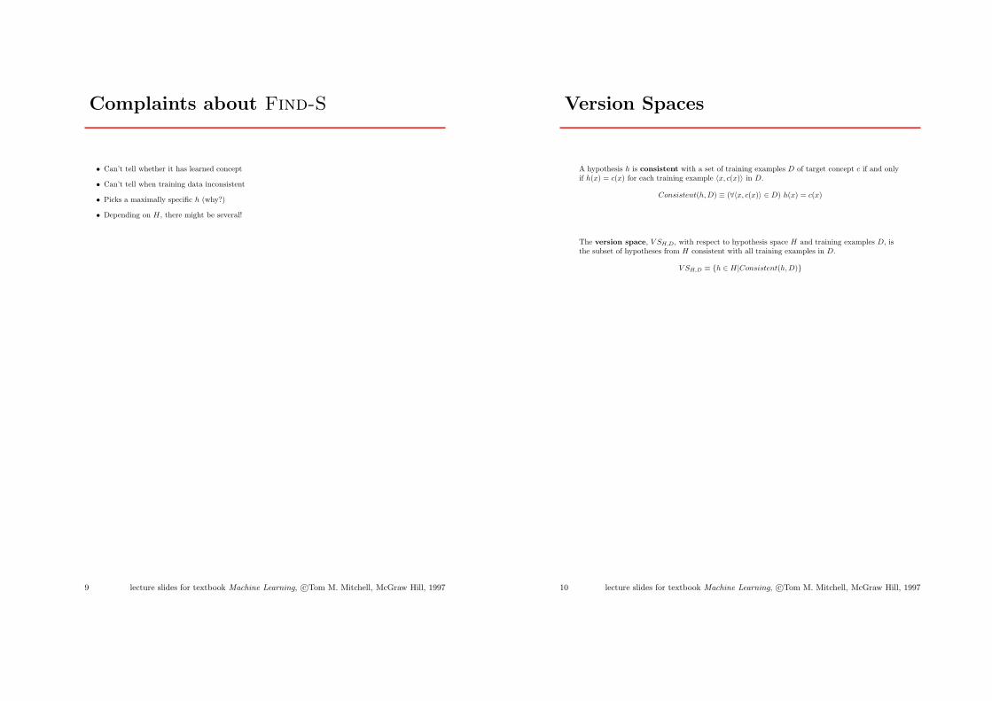
Complaints about Find-S

• Can’t tell whether it has learned concept

• Can’t tell when training data inconsistent

• Picks a maximally specific h (why?)

• Depending on H , there might be several!


Version Spaces

A hypothesis h is consistent with a set of training examples D of target concept c if and onlyif h(x) = c(x) for each training example ⟨x, c(x)⟩ in D.

Consistent(h,D) ≡ (∀⟨x, c(x)⟩ ∈ D) h(x) = c(x)

The version space, V SH,D, with respect to hypothesis space H and training examples D, isthe subset of hypotheses from H consistent with all training examples in D.

V SH,D ≡ {h ∈ H |Consistent(h,D)}


The List-Then-Eliminate Algorithm:

1. V ersionSpace← a list containing every hypothesis in H

2. For each training example, ⟨x, c(x)⟩

remove from V ersionSpace any hypothesis h for which h(x) ̸= c(x)

3. Output the list of hypotheses in V ersionSpace


Example Version Space


S:

<Sunny, Warm, ?, ?, ?, ?><Sunny, ?, ?, Strong, ?, ?> <?, Warm, ?, Strong, ?, ?>

<Sunny, Warm, ?, Strong, ?, ?>{ }

G: <Sunny, ?, ?, ?, ?, ?>, <?, Warm, ?, ?, ?, ?> { }


Concept Learning As Search


• # instances

– 3× 2× 2× 2× 2× 2 = 96

• # classifications

– 296

• # syntactically distinct hypotheses

– 5120

• ⟨., .,φ, ., ., .⟩

– represents no instance

• # semantically distinct hypotheses

– 975

When large hypothesis space H (possibly infinite) then efficient search strategies required to findhypothesis that best fits the data.


Representing Version Spaces

The General boundary, G, of version space V SH,D is the set of its maximally general members

The Specific boundary, S, of version space V SH,D is the set of its maximally specific members

Every member of the version space lies between these boundaries

V SH,D = {h ∈ H |(∃s ∈ S)(∃g ∈ G)(g ≥ h ≥ s)}

where x ≥ y means x is more general or equal to y


Candidate Elimination Algorithm

G← maximally general hypotheses in H , ⟨?, ?, ?, ?, ?, ?⟩S ← maximally specific hypotheses in H , ⟨φ,φ,φ,φ,φ,φ⟩For each training example d, do

• If d is a positive example

– Remove from G any hypothesis inconsistent with d

– For each hypothesis s in S that is not consistent with d

∗ Remove s from S

∗ Add to S all minimal generalizations h of s such that

1. h is consistent with d, and

2. some member of G is more general than h

∗ Remove from S any hypothesis that is more general than another hypothesis in S

• If d is a negative example

– Remove from S any hypothesis inconsistent with d

– For each hypothesis g in G that is not consistent with d

∗ Remove g from G

∗ Add to G all minimal specializations h of g such that

1. h is consistent with d, and

2. some member of S is more specific than h

∗ Remove from G any hypothesis that is less general than another hypothesis in G


Example Trace

{<?, ?, ?, ?, ?, ?>}

S0:{<Ø, Ø, Ø, Ø, Ø, Ø>}

G0:


What Next Training Example?

S:



G: <Sunny, ?, ?, ?, ?, ?>, <?, Warm, ?, ?, ?, ?> { }

What query is best, most informative?

A query is satisfied by # / 2 of the hypotheses, and not satisfied by the other half

For example⟨Sunny,Warm,Normal, Light,Warm, Same⟩

Note: Answer comes from nature or teacher# experiments: log2 |V S|


How Should These Be Classified?

S:



G: <Sunny, ?, ?, ?, ?, ?>, <?, Warm, ?, ?, ?, ?> { }

⟨Sunny Warm Normal Strong Cool Change⟩

⟨Rainy Cool Normal Light Warm Same⟩

⟨Sunny Warm Normal Light Warm Same⟩

⟨Sunny Cold Normal Strong Warm Same⟩


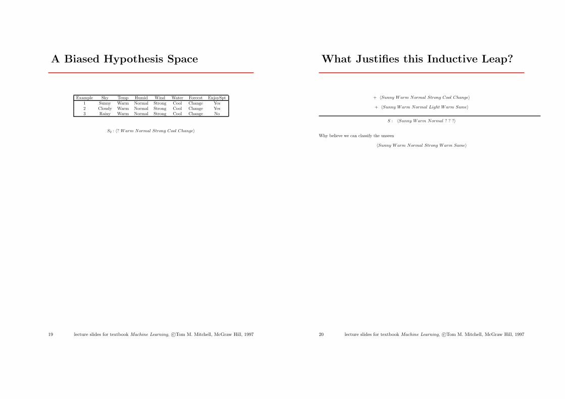
A Biased Hypothesis Space

Example Sky Temp Humid Wind Water Forecst EnjoySpt1 Sunny Warm Normal Strong Cool Change Yes2 Cloudy Warm Normal Strong Cool Change Yes3 Rainy Warm Normal Strong Cool Change No

S2 : ⟨? Warm Normal Strong Cool Change⟩


What Justifies this Inductive Leap?

+ ⟨Sunny Warm Normal Strong Cool Change⟩

+ ⟨Sunny Warm Normal Light Warm Same⟩

S : ⟨Sunny Warm Normal ? ? ?⟩

Why believe we can classify the unseen

⟨Sunny Warm Normal Strong Warm Same⟩


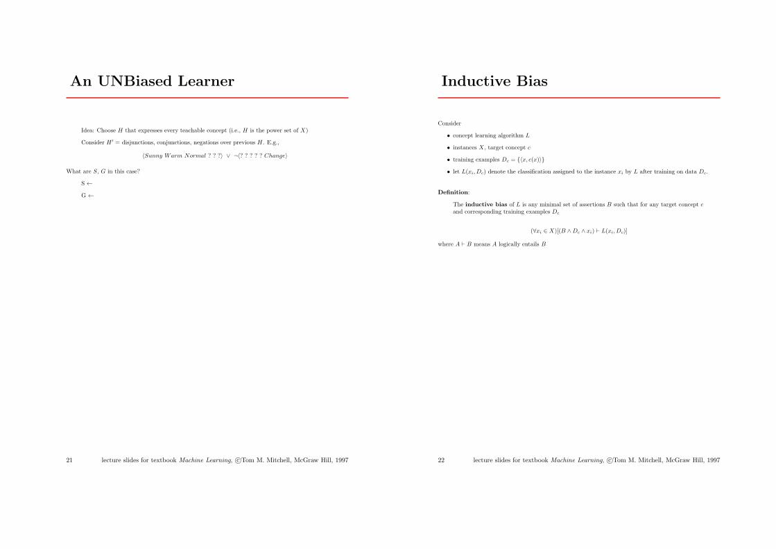
An UNBiased Learner

Idea: Choose H that expresses every teachable concept (i.e., H is the power set of X)

Consider H ′ = disjunctions, conjunctions, negations over previous H . E.g.,

⟨Sunny Warm Normal ? ? ?⟩ ∨ ¬⟨? ? ? ? ? Change⟩

What are S, G in this case?

S ←

G ←


Inductive Bias

Consider

• concept learning algorithm L

• instances X , target concept c

• training examples Dc = {⟨x, c(x)⟩}

• let L(xi, Dc) denote the classification assigned to the instance xi by L after training on data Dc.

Definition:

The inductive bias of L is any minimal set of assertions B such that for any target concept cand corresponding training examples Dc

(∀xi ∈ X)[(B ∧Dc ∧ xi) ⊢ L(xi, Dc)]

where A ⊢ B means A logically entails B


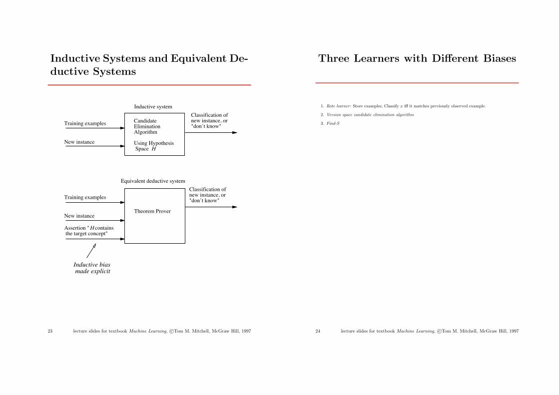
Inductive Systems and Equivalent De-ductive Systems

CandidateEliminationAlgorithm

Using Hypothesis Space

Training examples

New instance

Equivalent deductive system

Theorem Prover

Training examples

New instance

Inductive bias made explicit

Classification of new instance, or"don’t know"

Classification of new instance, or"don’t know"

Inductive system

H

Assertion " contains the target concept"

H


Three Learners with Different Biases

1. Rote learner: Store examples, Classify x iff it matches previously observed example.

2. Version space candidate elimination algorithm

3. Find-S


Summary Points

1. Concept learning as search through H

2. General-to-specific ordering over H

3. Version space candidate elimination algorithm

4. S and G boundaries characterize learner’s uncertainty

5. Learner can generate useful queries

6. Inductive leaps possible only if learner is biased

7. Inductive learners can be modelled by equivalent deductive systems


Decision Tree Learning

[read Chapter 3][recommended exercises 3.1, 3.4]

• Decision tree representation

• ID3 learning algorithm

• Entropy, Information gain

• Overfitting


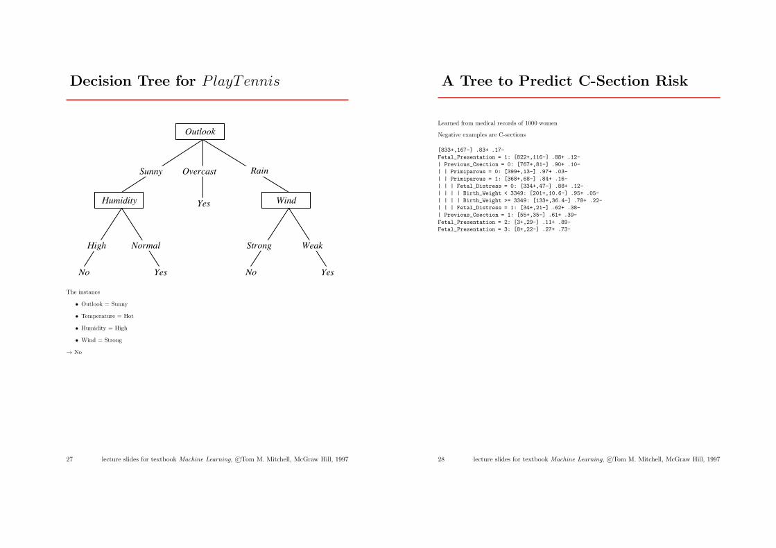
Decision Tree for PlayTennis

Outlook

Overcast

Humidity

NormalHigh

No Yes

Wind

Strong Weak

No Yes

Yes

RainSunny

The instance

• Outlook = Sunny

• Temperature = Hot

• Humidity = High

• Wind = Strong

→ No


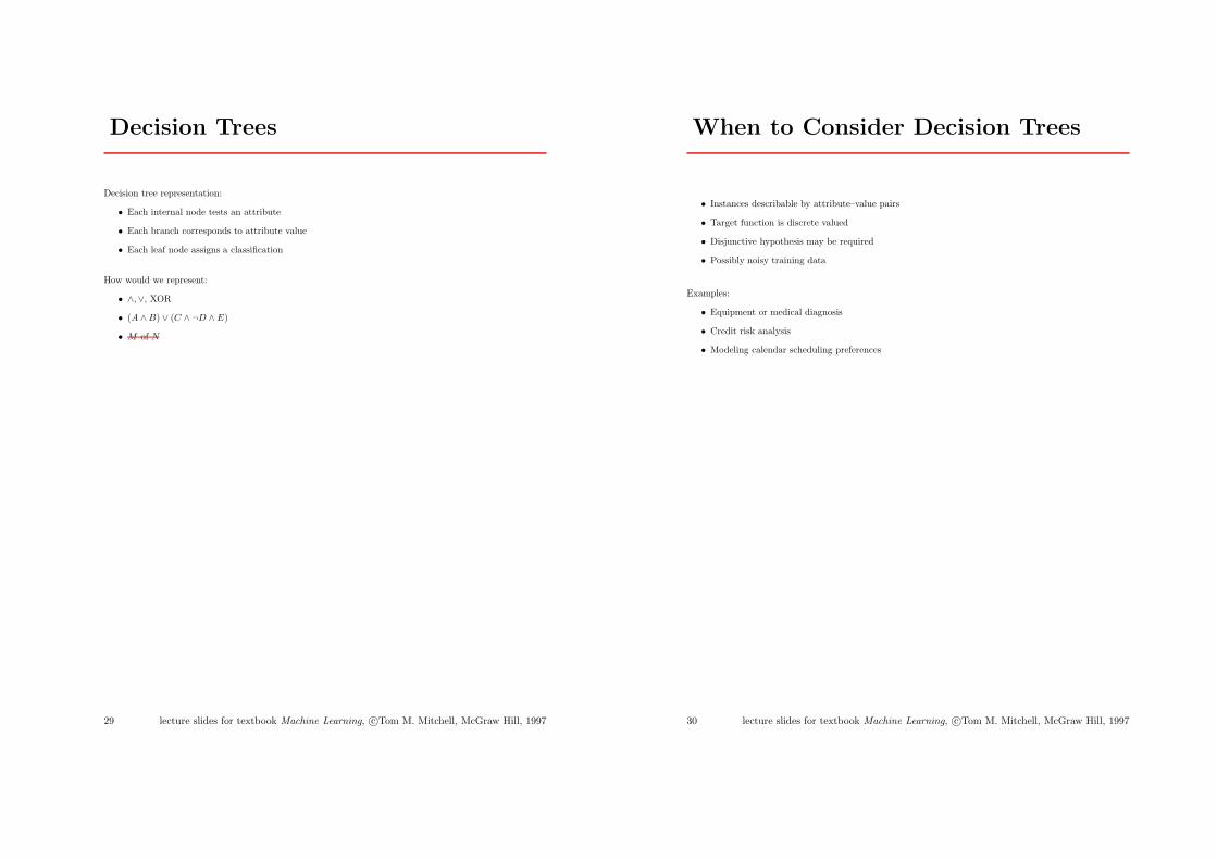
A Tree to Predict C-Section Risk

Learned from medical records of 1000 women

Negative examples are C-sections

[833+,167-] .83+ .17-Fetal_Presentation = 1: [822+,116-] .88+ .12-| Previous_Csection = 0: [767+,81-] .90+ .10-| | Primiparous = 0: [399+,13-] .97+ .03-| | Primiparous = 1: [368+,68-] .84+ .16-| | | Fetal_Distress = 0: [334+,47-] .88+ .12-| | | | Birth_Weight < 3349: [201+,10.6-] .95+ .05-| | | | Birth_Weight >= 3349: [133+,36.4-] .78+ .22-| | | Fetal_Distress = 1: [34+,21-] .62+ .38-| Previous_Csection = 1: [55+,35-] .61+ .39-Fetal_Presentation = 2: [3+,29-] .11+ .89-Fetal_Presentation = 3: [8+,22-] .27+ .73-


Decision Trees

Decision tree representation:

• Each internal node tests an attribute

• Each branch corresponds to attribute value

• Each leaf node assigns a classification

How would we represent:

• ∧,∨, XOR

• (A ∧B) ∨ (C ∧ ¬D ∧E)

• M of N


When to Consider Decision Trees

• Instances describable by attribute–value pairs

• Target function is discrete valued

• Disjunctive hypothesis may be required

• Possibly noisy training data

Examples:

• Equipment or medical diagnosis

• Credit risk analysis

• Modeling calendar scheduling preferences


Top-Down Induction of DecisionTrees

Main loop:

1. A← the “best” decision attribute for next node

2. Assign A as decision attribute for node

3. For each value of A, create new descendant of node

4. Sort training examples to leaf nodes

5. If training examples perfectly classified, Then STOP, Else iterate over new leaf nodes

Which attribute is best?

A1=? A2=?

ft ft

[29+,35-] [29+,35-]

[21+,5-] [8+,30-] [18+,33-] [11+,2-]


Entropy

Entro

py(S

)

1.0

0.5

0.0 0.5 1.0p+

• S is a sample of training examples

• p⊕ is the proportion of positive examples in S

• p⊖ is the proportion of negative examples in S

• Entropy measures the impurity of S

Entropy(S) ≡ −p⊕ log2 p⊕ − p⊖ log2 p⊖


Entropy

Entropy(S) = expected number of bits needed to encode class (⊕ or ⊖) of randomly drawn member of S(under the optimal, shortest-length code)

Why?

Information theory: optimal length code assigns − log2 p bits to message having probability p.

So, expected number of bits to encode ⊕ or ⊖ of random member of S:

p⊕(− log2 p⊕) + p⊖(− log2 p⊖)

Entropy(S) ≡ −p⊕ log2 p⊕ − p⊖ log2 p⊖

with c-wise classification, we get

Entropy(S) =c!

i=1

−pi log2 pi


Information Gain

Gain(S,A) = expected reduction in entropy due to sorting on A

Gain(S,A) ≡ Entropy(S) −!

v∈V alues(A)

|Sv||S|

Entropy(Sv)

A1=? A2=?

ft ft

[29+,35-] [29+,35-]

[21+,5-] [8+,30-] [18+,33-] [11+,2-]


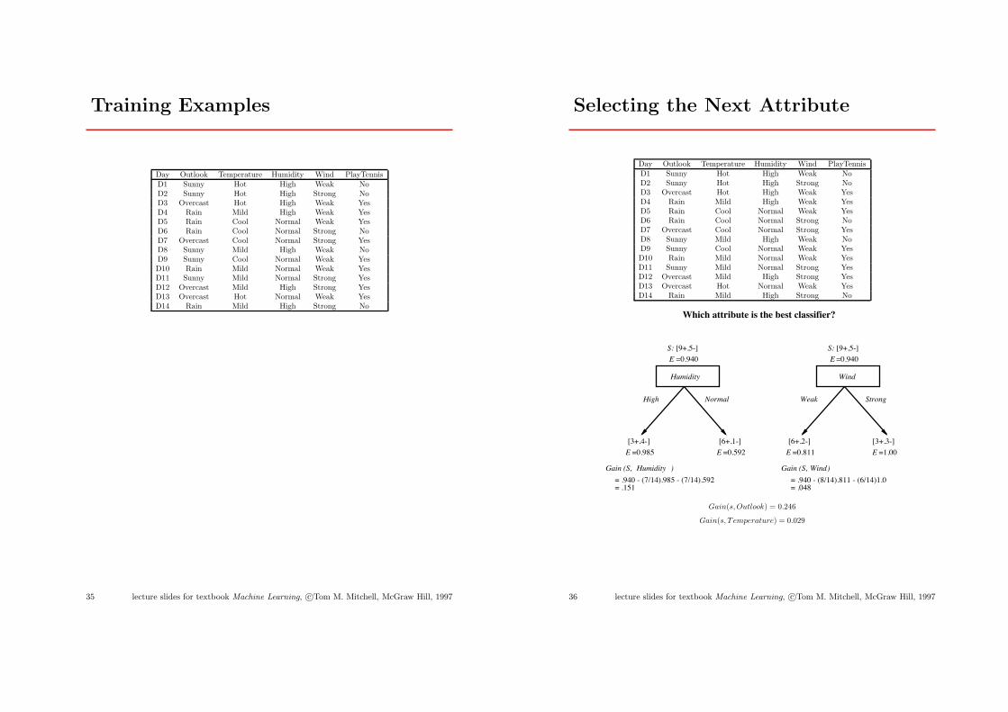
Training Examples

Day Outlook Temperature Humidity Wind PlayTennisD1 Sunny Hot High Weak NoD2 Sunny Hot High Strong NoD3 Overcast Hot High Weak YesD4 Rain Mild High Weak YesD5 Rain Cool Normal Weak YesD6 Rain Cool Normal Strong NoD7 Overcast Cool Normal Strong YesD8 Sunny Mild High Weak NoD9 Sunny Cool Normal Weak YesD10 Rain Mild Normal Weak YesD11 Sunny Mild Normal Strong YesD12 Overcast Mild High Strong YesD13 Overcast Hot Normal Weak YesD14 Rain Mild High Strong No


Selecting the Next Attribute

Day Outlook Temperature Humidity Wind PlayTennisD1 Sunny Hot High Weak NoD2 Sunny Hot High Strong NoD3 Overcast Hot High Weak YesD4 Rain Mild High Weak YesD5 Rain Cool Normal Weak YesD6 Rain Cool Normal Strong NoD7 Overcast Cool Normal Strong YesD8 Sunny Mild High Weak NoD9 Sunny Cool Normal Weak YesD10 Rain Mild Normal Weak YesD11 Sunny Mild Normal Strong YesD12 Overcast Mild High Strong YesD13 Overcast Hot Normal Weak YesD14 Rain Mild High Strong No

Which attribute is the best classifier?

High Normal

Humidity

[3+,4-] [6+,1-]

Wind

Weak Strong

[6+,2-] [3+,3-]

= .940 - (7/14).985 - (7/14).592 = .151

= .940 - (8/14).811 - (6/14)1.0 = .048

Gain (S, Humidity ) Gain (S, )Wind

=0.940E =0.940E

=0.811E=0.592E=0.985E =1.00E

[9+,5-]S:[9+,5-]S:

Gain(s,Outlook) = 0.246

Gain(s, T emperature) = 0.029


Outlook

Sunny Overcast Rain

[9+,5−]

{D1,D2,D8,D9,D11} {D3,D7,D12,D13} {D4,D5,D6,D10,D14}[2+,3−] [4+,0−] [3+,2−]

Yes

{D1, D2, ..., D14}

? ?

Which attribute should be tested here?

Ssunny = {D1,D2,D8,D9,D11}

Gain (Ssunny , Humidity)

sunnyGain (S , Temperature) = .970 − (2/5) 0.0 − (2/5) 1.0 − (1/5) 0.0 = .570

Gain (S sunny , Wind) = .970 − (2/5) 1.0 − (3/5) .918 = .019

= .970 − (3/5) 0.0 − (2/5) 0.0 = .970


Hypothesis Space Search by ID3

...

+ + +

A1

+ – + –

A2

A3+

...

+ – + –

A2

A4–

+ – + –

A2

+ – +

... ...

–

ID3 algorithms perform a single to complex hill-climbing searching

The evaluation function = information gain


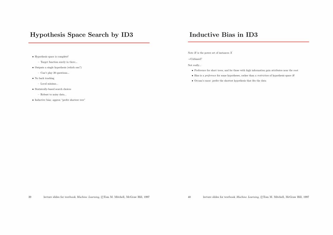
Hypothesis Space Search by ID3

• Hypothesis space is complete!

– Target function surely in there...

• Outputs a single hypothesis (which one?)

– Can’t play 20 questions...

• No back tracking

– Local minima...

• Statisically-based search choices

– Robust to noisy data...

• Inductive bias: approx “prefer shortest tree”


Inductive Bias in ID3

Note H is the power set of instances X

→Unbiased?

Not really...

• Preference for short trees, and for those with high information gain attributes near the root

• Bias is a preference for some hypotheses, rather than a restriction of hypothesis space H

• Occam’s razor: prefer the shortest hypothesis that fits the data


Occam’s Razor

Why prefer short hypotheses?

Argument in favor:

• Fewer short hyps. than long hyps.

→ a short hyp that fits data unlikely to be coincidence

→ a long hyp that fits data might be coincidence

Argument opposed:

• There are many ways to define small sets of hyps

• e.g., all trees with a prime number of nodes that use attributes beginning with “Z”

• What’s so special about small sets based on size of hypothesis??


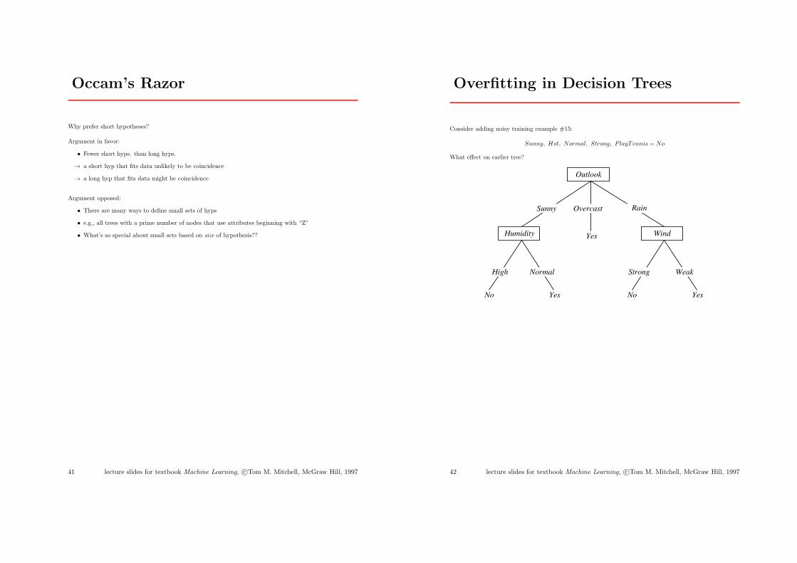
Overfitting in Decision Trees

Consider adding noisy training example #15:

Sunny, Hot, Normal, Strong, P layT ennis = No

What effect on earlier tree?

Outlook

Overcast

Humidity

NormalHigh

No Yes

Wind

Strong Weak

No Yes

Yes

RainSunny


Overfitting

Consider error of hypothesis h over

• training data: errortrain(h)

• entire distribution D of data: errorD(h)

Hypothesis h ∈ H overfits training data if there is an alternative hypothesis h′ ∈ H such that

errortrain(h) < errortrain(h′)

anderrorD(h) > errorD(h′)


Overfitting in Decision Tree Learning

0.5

0.55

0.6

0.65

0.7

0.75

0.8

0.85

0.9

0 10 20 30 40 50 60 70 80 90 100

Acc

urac

y

Size of tree (number of nodes)

On training dataOn test data


Avoiding Overfitting

How can we avoid overfitting?

• stop growing when data split not statistically significant

• grow full tree, then post-prune

How to select “best” tree:

• Measure performance over training data

• Measure performance over separate validation data set

• MDL: minimize size(tree) + size(misclassifications(tree))


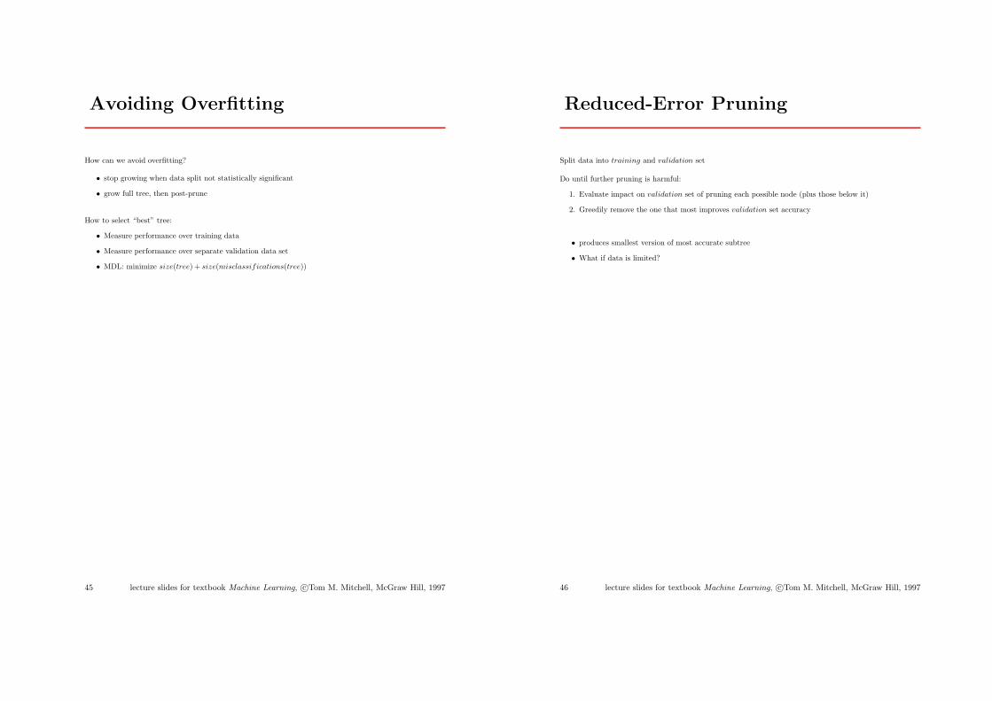
Reduced-Error Pruning

Split data into training and validation set

Do until further pruning is harmful:

1. Evaluate impact on validation set of pruning each possible node (plus those below it)

2. Greedily remove the one that most improves validation set accuracy

• produces smallest version of most accurate subtree

• What if data is limited?


Effect of Reduced-Error Pruning

0.5

0.55

0.6

0.65

0.7

0.75

0.8

0.85

0.9

0 10 20 30 40 50 60 70 80 90 100

Acc

urac

y

Size of tree (number of nodes)

On training dataOn test data

On test data (during pruning)


Rule Post-Pruning

1. Convert tree to equivalent set of rules

2. Prune each rule independently of others

3. Sort final rules into desired sequence for use

Perhaps most frequently used method (e.g., C4.5)


Converting A Tree to Rules

Outlook

Overcast

Humidity

NormalHigh

No Yes

Wind

Strong Weak

No Yes

Yes

RainSunny

IF (Outlook = Sunny) ∧ (Humidity = High)THEN PlayT ennis = No

IF (Outlook = Sunny) ∧ (Humidity = Normal)THEN PlayT ennis = Y es

. . .


Continuous Valued Attributes

Create a discrete attribute to test continuous

• Temperature = 82.5

• (Temperature > 72.3) = t, f

Temperature: 40 48 60 72 80 90PlayTennis: No No Yes Yes Yes No


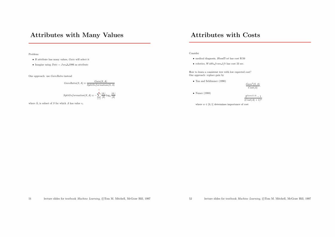
Attributes with Many Values

Problem:

• If attribute has many values, Gain will select it

• Imagine using Date = Jun 3 1996 as attribute

One approach: use GainRatio instead

GainRatio(S,A) ≡ Gain(S,A)

SplitInformation(S,A)

SplitInformation(S,A) ≡ −c!

i=1

|Si||S|

log2|Si||S|

where Si is subset of S for which A has value vi


v-

Attributes with Costs

Consider

• medical diagnosis, BloodTest has cost $150

• robotics, Width from 1ft has cost 23 sec.

How to learn a consistent tree with low expected cost?One approach: replace gain by

• Tan and Schlimmer (1990)Gain2(S,A)

Cost(A).

• Nunez (1988)2Gain(S,A) − 1

(Cost(A) + 1)w

where w ∈ [0, 1] determines importance of cost


Unknown Attribute Values

What if some examples missing values of A?Use training example anyway, sort through tree

• If node n tests A, assign most common value of A among other examples sorted to node n

• assign most common value of A among other examples with same target value

• assign probability pi to each possible value vi of A

– assign fraction pi of example to each descendant in tree

Classify new examples in same fashion


Documents

Outline Training Examples for EnjoySport learning and... · Sunny Warm High Strong Warm Same Yes ... Example Version Space Sky Temp Humid Wind Water Forecst EnjoySpt ... Three Learners