Embed Size (px)
Citation preview

September 3, 2013
Engineering Systems for Positioning and synchronizing and other amenitiesPaolo Carbone - University of Perugia - Italy
OutlineMotivations (why)Positioning & synchronizing (what)The measurement system (how we did it)Serendipity and lessons learned (some expected and unexpected consequences)
martedì 3 settembre 13
Blue sky research
✤ Characterization of communication networks
✤ Student’s project: measure length of a cable between two nodes of a sensor network
uC uC
Ping-pong approach of data packetsCount the number of bounces in 0.25sCOTS uC: max error < 20cm over 5 m
Cable in water ....Cable around your body ...Ranging in sensor networks? martedì 3 settembre 13

Ranging and positioning in sensor network systems✤ Ample scenario of ubiquitous computing and location-aware computing
✤ request for seamless localization capabilities inside and outside buildings
✤ Applications in areas such: emergency, safety, security, tracking, logistics, personal navigation, gaming, military, commerce
✤ Standardization driver: IEEE 802.15.4a-2007: Wireless Medium Access Control (MAC) and Physical Layer (PHY) Specifications for Low-Rate Wireless Personal Area Networks (WPANs)
✤ GPS does not provide useful information in closed environments and urban canyons
✤ Sister problem: network node synchronization
martedì 3 settembre 13

... driven by market needs
martedì 3 settembre 13
... an old problem
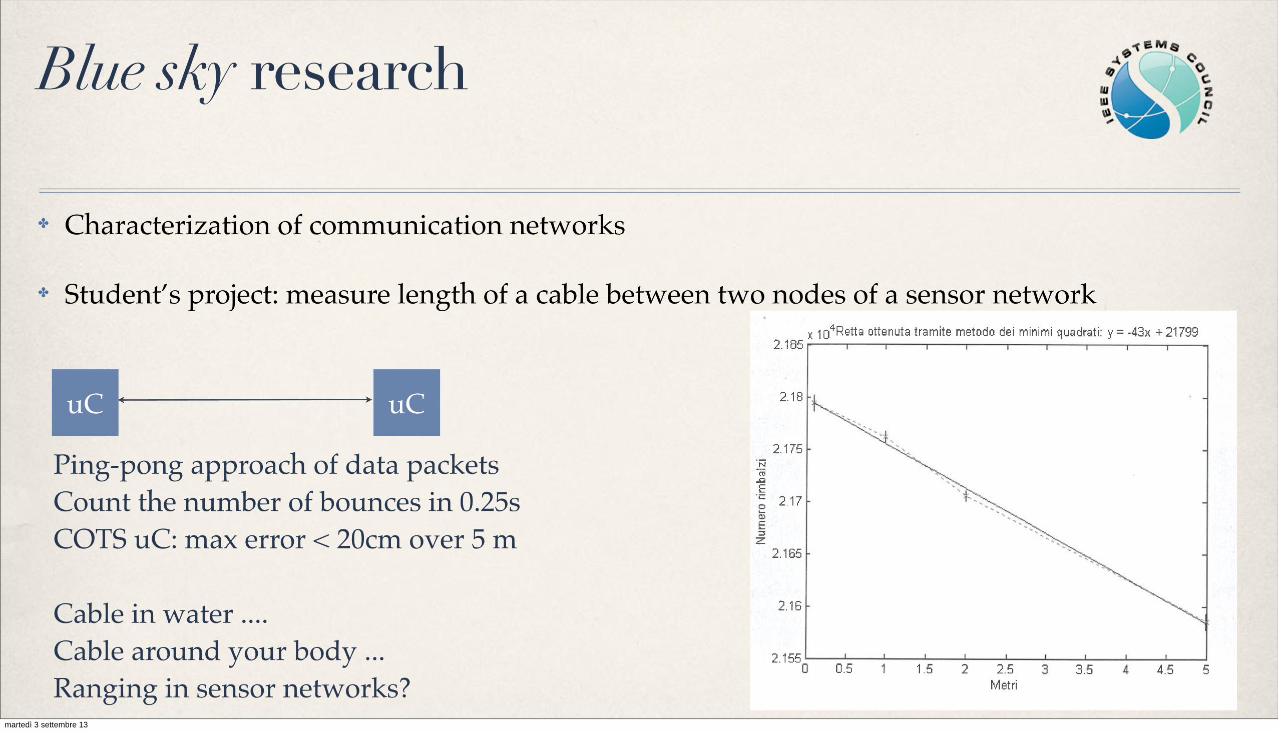
✤ compass (around 1000) and astrolabe, quadrant, sextant since 17th century
✤ navigation using the sun and the stars
✤ radar (half of 20th century)
martedì 3 settembre 13

Requirements andpossible technologies
Ultrasound• Optical/visual systems (infrared, laser, cameras)• Inertial navigation• RFID• Wi-Fi• UWB• ZigBeeHybridization of technologies
martedì 3 settembre 13
Measurement model
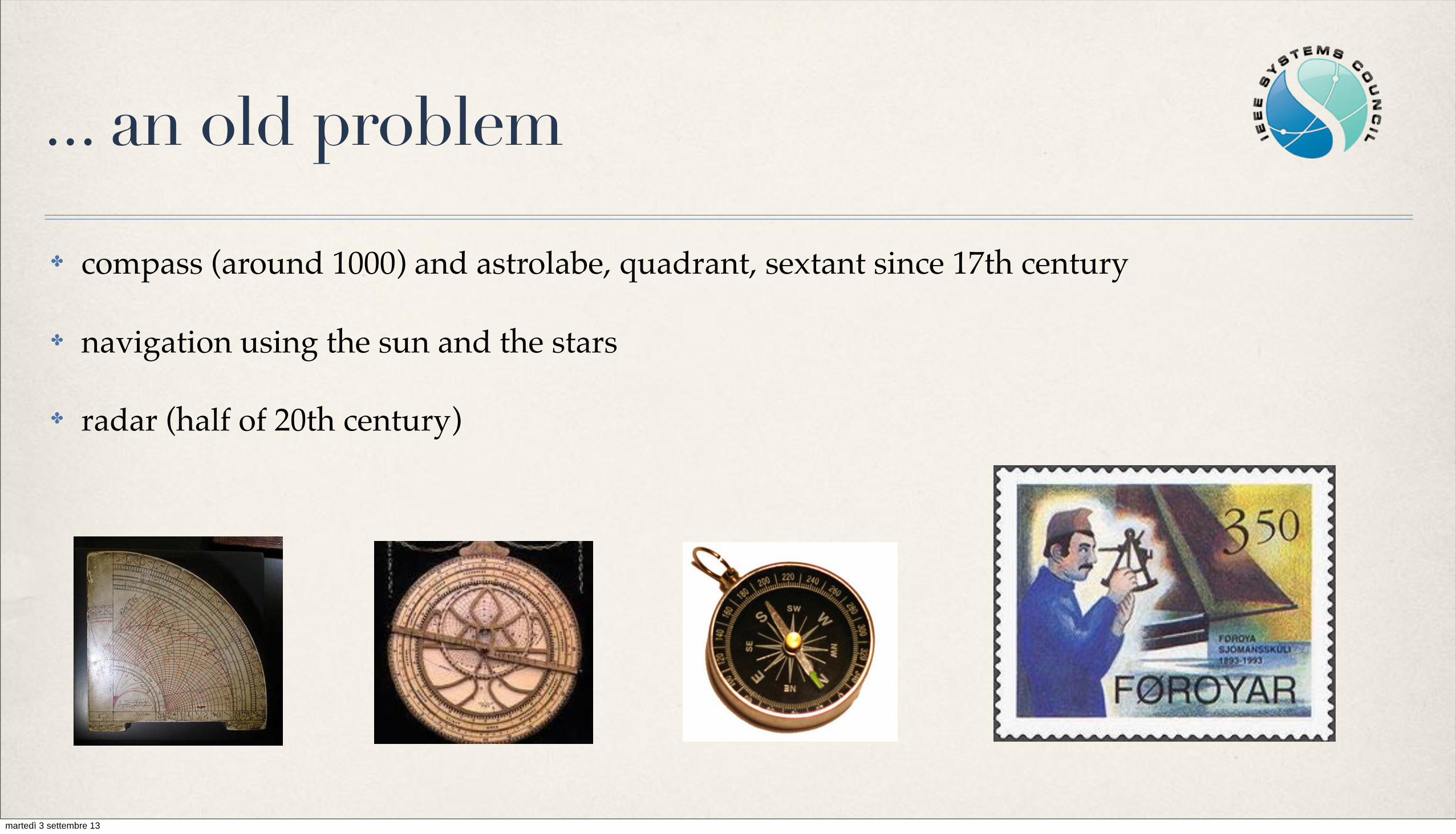
✤ Shadowing, multipath and NLOS effects influence measurement context
✤ UWB: very few full realizations described in literaturemartedì 3 settembre 13

Measurement methods
Many algorithms are applicable: NLS is the simplest one (others being Extended Kalman filtering, particle filtering, ...)
A triangulation problem
TOA - synchronization issues between M/S and clock granularityTDOA - synchronized slavesRTT - synchronization not neededAOA - requires directional antennas
fingerprinting (RSSI), video, tagging, pattern matching
martedì 3 settembre 13

The measurement system: a systems engineering challenge✤ Really a systems engineering type of problem:
✤ Much of the technology is known: difficulties at interfacing and synchronizing operations
✤ Sensor network: several slave nodes at known positions and the master node
✤ Generation of very short-time pulses (<1 ns rise time)
✤ measurement short-time intervals (with <100 ps accuracy)
✤ synchronization and communication between nodes
✤ management of signals and application of signal processing
martedì 3 settembre 13

System overview
✤ System Architecture
Metrol. Meas. Syst., Vol. XVII (2010), No. 3, pp. 447-460
[15] and in [16], including a description of the main system characteristics from a system-level point of view. Furthermore, an in-depth discussion on the signal processing techniques used and the related issues have been presented in [17]. 1.5. Outline
The outline of the paper is as follows. In Section 2, a system overview is presented and the main features of the UWB radio positioning subsystem and the INS are outlined. Thereafter, in Section 3, the sensor fusion of the information provided by the two sources is discussed. In Section 4, the experimental setup used to test the system and the test results are presented. Finally, in Section 5, conclusions regarding the work are drawn. 2. System overview
The indoor navigation system consists of the infrastructure segment and the user segment. It is schematically presented in Fig. 1.
Fig. 1. Functional diagram of the complete Fig. 2. Architecture of the UWB master indoor positioning system [15]. device [15].
The infrastructure segment comprises a set of UWB radio nodes located at known
positions within the operational area. The user segment is the navigation unit, which aims to estimate its location and attitude relative to the UWB radio nodes by combining UWB radio range measurements and inertial navigation. To achieve this task, the navigation unit comprises: − An UWB ranging device (master unit, see Section 2.1) measuring the ranges to UWB
radio nodes (slave units, see Section 2.1). − An inertial measurement unit (IMU) providing acceleration and angular rate
measurements for the INS. − A PC running the mechanization equations of the INS and an extended Kalman filter
(EKF); where the EKF is used to combine the information from the INS with the measurements of the UWB ranging system, yielding a joint navigation solution.
2.1. Ultra wide band radio distance measurements
The principle of operation of the UWB ranging system is based on the indirect measurement of the distance between transceivers, obtained by measuring the round-trip time (RTT) of an UWB pulse [5]. This approach does not require temporal synchronization, which is an advantage when compared to other commonly used strategies such as time-of-arrival or time-difference-of-arrival [1, 4]. However, when measuring the RTT, the latency introduced by the responder devices has to be accurately measured or estimated. In the present system, this issue is addressed by performing a calibration of each slave unit [15, 18].
449
✤ Master/slave units
martedì 3 settembre 13

System operations
✤ Round robin selection of slave device as transponders
A. De Angelis et al.: INDOOR POSITIONING BY ULTRAWIDE BAND RADIO AIDED INERTIAL NAVIGATION
The system is comprised of a master device and several slaves. The master transceiver is capable of measuring RTT. This time interval measuring function is performed by a commercial time-to-digital converter (TDC) integrated circuit, the TDC-GP2 by Acam Messelectronic GmbH, with a root-mean-square (RMS) resolution of 50 ps. A block diagram of the master is shown in Fig. 2. The slave devices are not designed to perform time interval measurements; but will instead − on request after a fixed delay − echo a UWB pulse with another UWB pulse, thus providing a “round trip”. The slave unit has two modes of operation: communication mode and responder mode. Fig. 3a shows a functional block diagram of the devices in communication mode, whilst the responder mode is illustrated in Fig. 3b. Using logic circuits, the slave devices switch between the two modes of operation. The circuit architectures of both the master and the slave devices are based on the system presented in [19], whilst the UWB pulse generator modules have been built using step recovery diodes using the circuit design presented in [20]. a) b)
Fig. 3. Simplified architecture of the slaves in the two operating modes: a) communication mode; b) responder mode [15].
Furthermore, omnidirectional wideband disc-cone antennae have been used in the
receiving and transmitting sections of each device. Fig. 4 shows a picture of one of the realized prototypes.
Fig. 4. Picture of the realized Fig. 5. Operation of the system, prototype of the master device [15]. showing the addressing and measurement phases, together with timing information [15].
An example of timing diagram for the operation of the system is provided in Fig. 5. It is
divided in two sequential phases − addressing and measurement. In the first phase, the master sends an 8-bit unique slave identifier code, using on-off keying with UWB pulses. In this basic modulation scheme, if a pulse is transmitted within a specific time slot, it is interpreted as a “1” bit. The absence of a pulse is seen as a “0” bit. During the addressing phase all the
450
✤ One of the realized master unit prototypes
martedì 3 settembre 13

How we did it
✤ Ultra wide-bandwidth pulses (UWB): relative bandwidth > 20% or absolute bandwidth > 500 MHz. Preferred because of:
✤ fine time resolution, < 1ns rise time
✤ robustness to multipath
✤ low power generation
✤ lab synthesis of UWB pulses: critical path in digital ports to generate short-delays and artificial glitches, step-recovery diode, avalanche diode
martedì 3 settembre 13
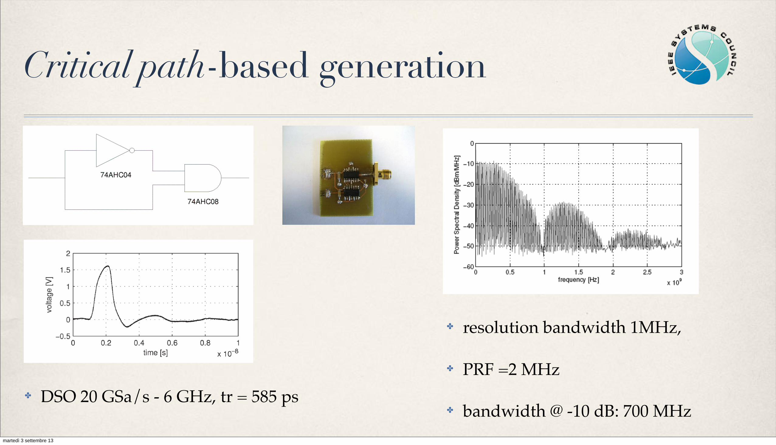
Critical path-based generation
✤ DSO 20 GSa/s - 6 GHz, tr = 585 ps
✤ resolution bandwidth 1MHz,
✤ PRF =2 MHz
✤ bandwidth @ -10 dB: 700 MHzmartedì 3 settembre 13
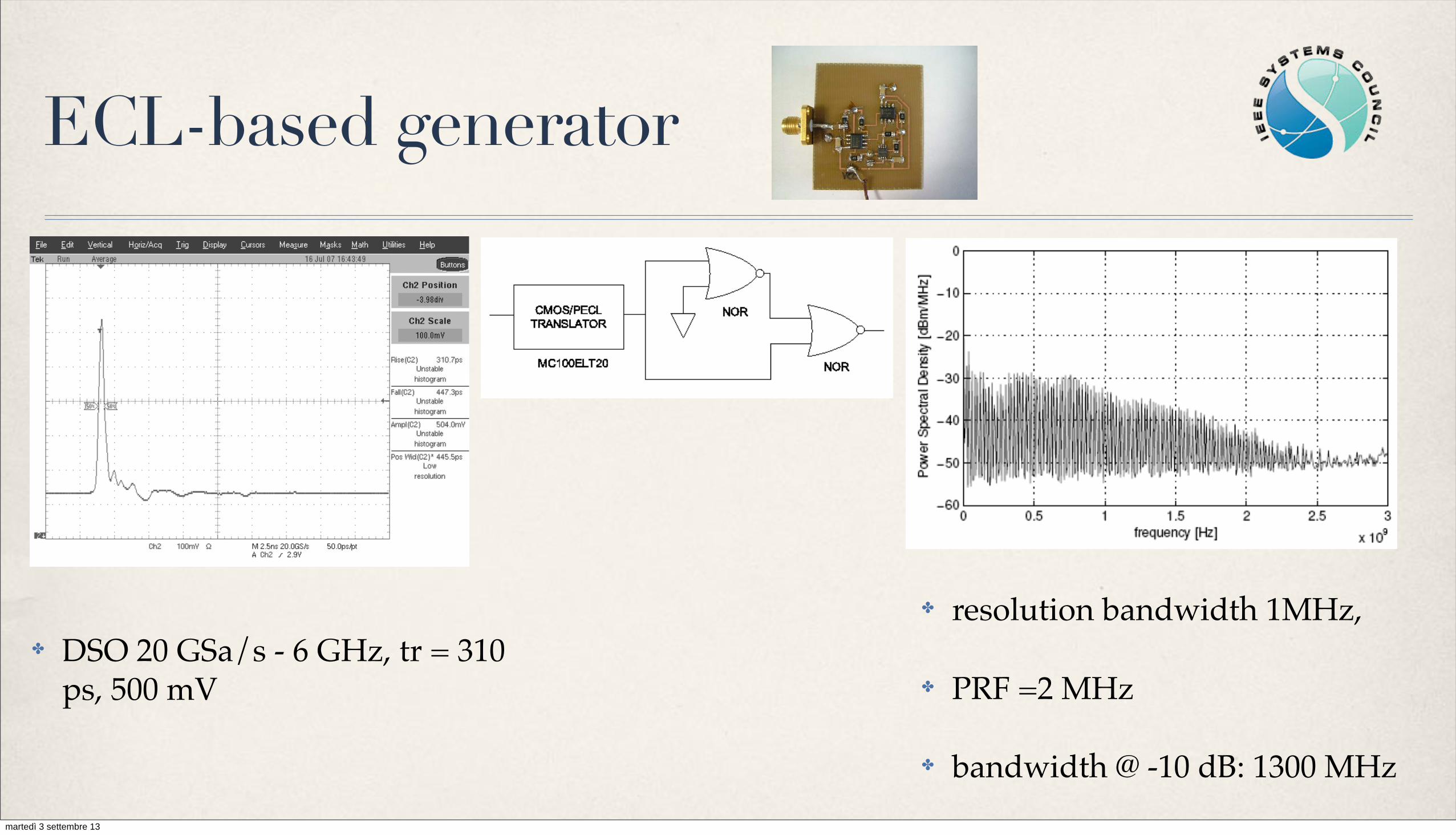
ECL-based generator
✤ DSO 20 GSa/s - 6 GHz, tr = 310 ps, 500 mV
✤ resolution bandwidth 1MHz,
✤ PRF =2 MHz
✤ bandwidth @ -10 dB: 1300 MHzmartedì 3 settembre 13
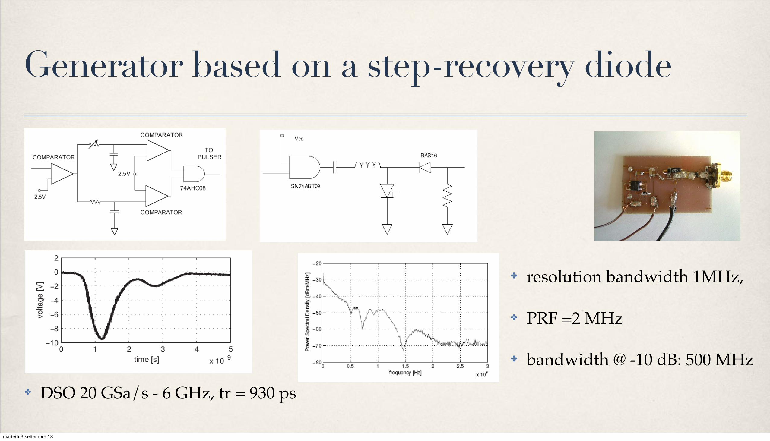
Generator based on a step-recovery diode
✤ DSO 20 GSa/s - 6 GHz, tr = 930 ps
✤ resolution bandwidth 1MHz,
✤ PRF =2 MHz
✤ bandwidth @ -10 dB: 500 MHz
martedì 3 settembre 13

Avalanche-based flasher
✤ Large amplitude pulses
✤ high voltage needed to put BJT in avalanche mode
martedì 3 settembre 13

Modulated pulses✤ To reduce antenna size and better comply with masks regarding frequency emissions, we
modulated pulses using 5.6 GHz carrier and a mixer
✤ Sampling oscilloscope: 20 GHz bandwidth, 10 MSa/s, external triggering
martedì 3 settembre 13

Modulated pulses: measurements
✤ AHC pulser, 20 MHz PRF, bandwidth about equal to 1 GHz
310 IEEE TRANSACTIONS ON INSTRUMENTATION AND MEASUREMENT, VOL. 60, NO. 1, JANUARY 2011
Experimental Comparison of Low-CostSub-Nanosecond Pulse Generators
Alessio De Angelis, Member, IEEE, Marco Dionigi, Riccardo Giglietti, and Paolo Carbone, Senior Member, IEEE
Abstract—In this paper, six low-cost pulse generator deviceshaving sub-nanosecond transition time are analyzed and com-pared. Some of the possible applications for these devices are alsodescribed, along with an overview of the different approachesfor sub-nanosecond pulse generation. Furthermore, the architec-ture and principle of operation of the realized prototypes areexplained. The considered pulse generation techniques are basedon logic gates, Step-Recovery Diodes, and transistors driven in theavalanche region. Some experimental results obtained by usingan equivalent-time sampling oscilloscope and a spectrum analyzerare shown and discussed, providing both a time-domain and afrequency-domain characterization of the prototypes. Finally, anapproach for the generation of modulated pulses in the 6-GHzband (for ultra-wideband applications) is investigated, and exper-imental results are provided.
Index Terms—Experimental characterization, pulse generation,pulse measurements, ultra-wideband signals.
I. INTRODUCTION
SHORT-PULSE generation has applications in several areas,such as the following: 1) linear systems characterization;
2) time-domain reflectometry (TDR); and 3) ultra-wideband(UWB) systems. The characterization of linear systems reliessubstantially on the determination of their pulse response.Knowledge of an instrument’s pulse response can be usedto determine instrument performance and to compensate fornon-ideal behaviors. As an example, the pulse response of adigital oscilloscope can be determined by measuring a properly-characterized fast pulse [1], having a much greater bandwidththan that of the oscilloscope under test. The measured spectrumcontains harmonic sinusoidal components over the frequencyrange of interest (the oscilloscope’s bandwidth). From theknown pulse shape and the recorded oscilloscope responsewaveforms, the amplitude and phase of each Fourier harmoniccomponent can be obtained using the Discrete Fourier Trans-form. Finally, the impulse response can be determined by thedeconvolution of these two signals [2].
Manuscript received October 20, 2009; revised December 23, 2009; acceptedDecember 26, 2009. Date of publication May 17, 2010; date of current versionDecember 8, 2010. This work was supported in part by the Research GrantCARBIBRID, provided by the Fondazione Cassa di Risparmio di Terni, whosesupport the authors gratefully acknowledge. The Associate Editor coordinatingthe review process for this paper was Dr. V. R. Singh.
The authors are with the Department of Electronic and Information Engineer-ing (DIEI), University of Perugia, 06125 Perugia, Italy (e-mail: [email protected]; [email protected]; [email protected]; [email protected]).
Color versions of one or more of the figures in this paper are available onlineat http://ieeexplore.ieee.org.
Digital Object Identifier 10.1109/TIM.2010.2047591
Short pulse generators are commonly used in TDR systemsto characterize long transmission lines and detect failures orpotential problems. By analyzing pulse reflections, in fact, theimpedance changes can be localized within the transmissionline with high accuracy. This technique has also been applied tolocalize failures in printed circuit board traces or integrated cir-cuit packages [3]. Short-pulse properties can also be exploitedfor material characterization [4], [5].
Another application area for fast-pulse generation is UWBsystems, where sub-nanosecond pulse generation is one of themain issues. FCC First Report and Order of 2002 [6] definesan UWB system as any intentional radiator having a fractionalbandwidth greater than 20% or an absolute bandwidth greaterthan 500 MHz. The origin of UWB technology dates back tothe early 1960s within time-domain electromagnetics. After45 years of technological advancement, UWB systems havebeen used in several application fields [7], such as:
• radar systems with high-range measurement accuracy andresolution;
• high-data rate, short-range communication systems;• sensor networks for indoor geolocation;• ground-penetrating radars.
UWB systems offer several advantages compared to tradi-tional systems. First of all, they are a base-band technology; andconsequently, an impulse-based UWB receiver does not needan intermediate frequency stage, thus, widely reducing systemcomplexity and cost. Moreover, the signal power is spread overa wide range of frequencies, with an extremely low powerspectral density. This ensures small interference to other narrowband radio frequency (RF) signals and maintains excellentimmunity to interference from these signals. Therefore, UWBdevices can work within frequency intervals allocated for otherRF systems. This characteristic, along with their immunity tomultipath phenomena, makes UWB signals good candidates forseveral indoor applications.
Among the short pulses, the monocycle pulse is of partic-ular interest, since it presents a wideband spectrum withoutlow-frequency and DC components, simplifying the design ofvarious elements such as amplifiers and antennas [8]. Severalapproaches have been proposed to produce monocycle pulses[9]–[12]. In particular, the pulse-generating network can berealized with a full-custom approach based on CMOS technol-ogy, mainly for low-cost, low-power consumption, and easyintegration in digital or mixed integrated circuits [9], [13].This approach eases the implementation of tuning capabilitiesfor the generation of pulses of different duration, that is a
0018-9456/$26.00 © 2010 IEEE
DE ANGELIS et al.: EXPERIMENTAL COMPARISON OF LOW-COST SUBNANOSECOND PULSE GENERATORS 313
Fig. 8. Diagram of the modulator circuit: a 5.8-GHz VCO provides the carriersinewave, which is then amplified and connected to the mixer LO port. Thebase-band pulse (generated by the AHC or ECL device) is connected to themixer IF port, while the RF port provides the output modulated pulse.
Fig. 9. Picture of the realized prototypes: (a) AHC, (b) first ECL, (c) secondECL, (d) SRD, (e) Avalanche, (f) Microstrip pulse shaper, (g) Mixer.
Fig. 10. Measurement setup, in the output triggering configuration.
1.6-mm-thick FR-4 Glass Epoxy substrate. Furthermore, aground plane has been used to reduce the effects of interfer-ences. Where available, surface mount components have beenchosen, to minimize stray inductances. The width of the outputtrace has been calculated to obtain an output impedance of50 !. Fig. 9 shows a picture of the realized prototypes.
The devices have been characterized using an equivalent-time sampling oscilloscope with an analog bandwidth of20 GHz. Due to the maximum peak voltage specification of thisinstrument, some attenuators were used. However, the attenua-tion is compensated internally in the instrument. Furthermore,an external trigger signal was required by the sampling oscillo-scope. In order to provide such a signal while minimizing thetiming jitter, the measurement setup shown in Fig. 10 has beenadopted. The pulse generator output port has been connected,by means of a coaxial T-connector, to the sampling input andto the trigger channel of the instrument, as shown in Fig. 10. Itcan be noticed that both channels are characterized by an inputimpedance of 50 !, therefore, the amplitude of the waveformshown by the instrument is relative to an impedance of 25 !.This measuring setup will be referred to as “output-triggering”in the following sections of this paper.
Fig. 11. Comparison between input-triggering and output-triggering configu-rations. It can be noticed that the waveform acquired with the output-triggeringsetup shows a decreased timing jitter and noise level.
Fig. 12. AHC output acquired with 20-dB attenuation.
Fig. 13. ECL output acquired with 10-dB attenuation.
Initially, another measurement setup has been considered.Using this alternative setup, the input of the pulse generatoris connected to the sampling oscilloscope trigger. This config-uration has the drawback of increasing jitter, since the noiseand timing jitter introduced by the pulse generator are visiblein the acquired waveform. Therefore, this alternative setup,referred to as “input-triggering,” has been discarded and theoutput-triggering configuration has been used for all the time-domain measurements described in this paper. A closeup of arising-edge waveform by the same device acquired with thetwo different setups is shown for comparison in Fig. 11. Thedifference in voltage range is motivated by the different loadimpedance seen by the pulse generator in the two measurementsetups.
Figs. 12–17 show the observed pulse generators waveforms.For the second ECL generator, results are also shown for theconfiguration using the pulse-shaping network (see Fig. 15).
To characterize the frequency-domain behavior of thesepulse generators, their output power spectral density (PSD)
DE ANGELIS et al.: EXPERIMENTAL COMPARISON OF LOW-COST SUBNANOSECOND PULSE GENERATORS 315
Fig. 21. Second ECL pulser with shaping network PSD, 10 dB attenuation(1 MHz resolution bandwidth, 20 MHz pulse repetition frequency). A !10 dBbandwidth of about 1 GHz has been observed, while the first zero is at about1.5 GHz.
Fig. 22. SRD pulser PSD, 10-dB attenuation (1-MHz resolution bandwidth,2-MHz pulse repetition frequency). A !10-dB bandwidth of about 500 MHzhas been observed.
Fig. 23. Avalanche pulser radiated PSD (3-MHz resolution bandwidth,100-kHz pulse repetition frequency).
by means of antennas. A wide band omnidirectional disc coneantenna was employed to transmit the pulse, while a receivingdirectional ridged-horn antenna was connected to the spectrumanalyzer. The obtained trace is shown in Fig. 23.
The sampling oscilloscope acquisition shown in Fig. 24 isrelative to the upconverting modulator applied to the AHCpulse generator, while Fig. 25 shows the measured output PSDwith 20-MHz pulse repetition frequency and 1-MHz resolutionbandwidth. Similarly, the acquisitions relative to the secondECL pulser are displayed in Figs. 26 and 27.
IV. METROLOGICAL CHARACTERIZATION
For each pulse generator, four parameters have been con-sidered: 1) rise time (tR); 2) fall time (tF ); 3) pulse width(tW ); and 4) peak-to-peak amplitude (Vpp). Using the notationand guidance provided by the Guide to the Expression of
Fig. 24. Modulated AHC pulse.
Fig. 25. PSD of the AHC pulser output mixed with the 5.8-GHz carrier(1-MHz resolution bandwidth, 20-MHz pulse repetition frequency). Theobserved main lobe width, between the first zeros of the spectrum, is approxi-mately 1 GHz.
Fig. 26. Modulated second ECL pulse.
Fig. 27. PSD of the second ECL pulser output mixed with the 5.8-GHzcarrier (1-MHz resolution bandwidth, 20-MHz pulse repetition frequency).The observed main lobe width, between the first zeros of the spectrum, isapproximately 5 GHz, while the !10-dB bandwidth is about 3 GHz.
Uncertainty in Measurement (GUM) [22], the Type A com-ponent of the standard uncertainty is evaluated by performingthe statistical analysis of a series of repeated observations.Therefore, in this paper, it has been obtained by calculating the
martedì 3 settembre 13

Time-to-digital conversionFrom curiosity driven research to problem-led research
'ZRGTKOGPVCN�4CFKQ�+PFQQT�2QUKVKQPKPI�5[UVGOU�$CUGF�QP�4QWPF�6TKR�6KOG�OGCUWTGOGPV ���
ȱ)LJ�����3ULQFLSOH�RI�RSHUDWLRQ�RI�WKH�577�GLVWDQFH�PHDVXUHPHQW�DSSURDFK���7KH�PRVW� FRPPRQ�VWUDWHJ\� IRU�JHRORFDWLRQ�XVLQJ�=LJ%HH� VLJQDOV� LV�EDVHG�RQ� WKH�5HFHLYHG�6LJQDO�6WUHQJWK��566��RI�FRPPXQLFDWLRQ�VLJQDOV��%OXPHQWKDO�HW�DO����������&KR�HW�DO����������8VLQJ� WKLV� DSSURDFK�� DQ� HVWLPDWH� RI� WKH� GLVWDQFH� EHWZHHQ� D� WUDQVPLWWHU� DQG� D� UHFHLYHU� LV�REWDLQHG�E\�PHDQV�RI�WKH�UHFHLYHG�SRZHU�OHYHO��JLYHQ�DQ�DSSURSULDWH�PRGHO�IRU�WKH�SRZHU�ORVV� RI� WKH� WUDQVPLVVLRQ� FKDQQHO�� 6XFK� D�PHDVXUH�PD\� EH� SURYLGHG� E\� VRPH� FRPPHUFLDO�=LJ%HH�KDUGZDUH�DV�D�566�,QGLFDWRU��566,���+RZHYHU��WKH�DFKLHYDEOH�DFFXUDF\�RI�566�EDVHG�=LJ%HH�SRVLWLRQLQJ�V\VWHPV�LV�XVXDOO\�LQ�WKH�RUGHU�RI�PDJQLWXGH�RI���P���%HWWHU�UHVXOWV�FDQ�SRWHQWLDOO\� EH� REWDLQHG� ZLWK� 7LPH�2I�$UULYDO� PHWKRGV�� DV� GHPRQVWUDWHG� E\� VRPH� ZRUNV�IRXQG�LQ�WKH�OLWHUDWXUH��6DQWLQHOOL�HW�DO����������&RUUDO�HW�DO����������6FKZDU]HU�HW�DO����������
�����+PFQQT�4CFKQ�2TQRCICVKQP�%JCPPGN�2QH� RI� WKH� IXQGDPHQWDO� LVVXHV� DVVRFLDWHG� WR� UDGLR� JHRORFDWLRQ� LV� UHSUHVHQWHG� E\� WKH�SURSDJDWLRQ�FKDQQHO��,Q�IDFW��HVSHFLDOO\�LQ�LQGRRU�VFHQDULRV��WKH�FKDQQHO�LV�VWURQJO\�DIIHFWHG�E\� PXOWLSDWK� IDGLQJ�� D� SKHQRPHQRQ� ZKLFK� LV� RI� NH\� UHOHYDQFH� LQ� ERWK� WKH� DSSURDFKHV�FRQVLGHUHG�LQ�WKLV�ZRUN��,Q�SDUWLFXODU��IRU�WKH�8:%�FDVH��GXH�WR�WKH�KLJK�EDQGZLGWK�DQG�ILQH�WLPH�UHVROXWLRQ�RI�WKH�SXOVHV��WKH�V\VWHP�LV�LQWULQVLFDOO\�DEOH�WR�GLVFULPLQDWH�D�ODUJH�QXPEHU�RI�SDWKV��/HH��6FKROW]���������,Q�WKLV�ILHOG��FKDQQHO�PRGHOLQJ�UHVHDUFK�DFWLYLWLHV�KDYH�EHHQ�SXEOLVKHG� LQ� WKH� OLWHUDWXUH�� VHH� �0ROLVFK�� ������ �0ROLVFK� HW� DO��� ������� )XUWKHUPRUH�� WKH�=LJ%HH�VROXWLRQ�UHTXLUHV�DQ�HVVHQWLDOO\�GLIIHUHQW�DSSURDFK�WR�WKH�PXOWLSDWK�SUREOHP��VLQFH�LW�FDQ� EH� EDVLFDOO\� FRQVLGHUHG� DV� D� QDUURZEDQG� V\VWHP�� � ,Q� SDUWLFXODU�� DV� D� =LJ%HH� UHFHLYHU�UHOLHV� RQ� FRUUHODWLRQ� WHFKQLTXHV� WR� V\QFKURQL]H� LWVHOI� ZLWK� DQ� LQFRPLQJ� SDFNHW�� 577�PHDVXUHPHQWV�PD\�EH�DIIHFWHG�E\� LQFUHDVHG�FRUUHODWLRQ� WLPHV�ZKHQ� LQSXW� VLJQDO�SRZHU� LV�UHGXFHG�E\�PXOWLSDWK��7KH�JRDO�RI� UHVHDUFK�DFWLYLW\� LQ� WKLV� ILHOG� LV� WR�SURSHUO\�PRGHO�DQG�FRPSHQVDWH� WKLV� SKHQRPHQRQ�� LQ� RUGHU� WR� DFFXUDWHO\� HVWLPDWH� LWV� HIIHFW� RQ� WKH�PHDVXUHG�VLJQDO�WLPH�RI�IOLJKW��+LUVFKOHU�0DUFKDQG��+DWNH����������
Very first ranging experiments without TDC, as in the wired case then ... TDC
martedì 3 settembre 13
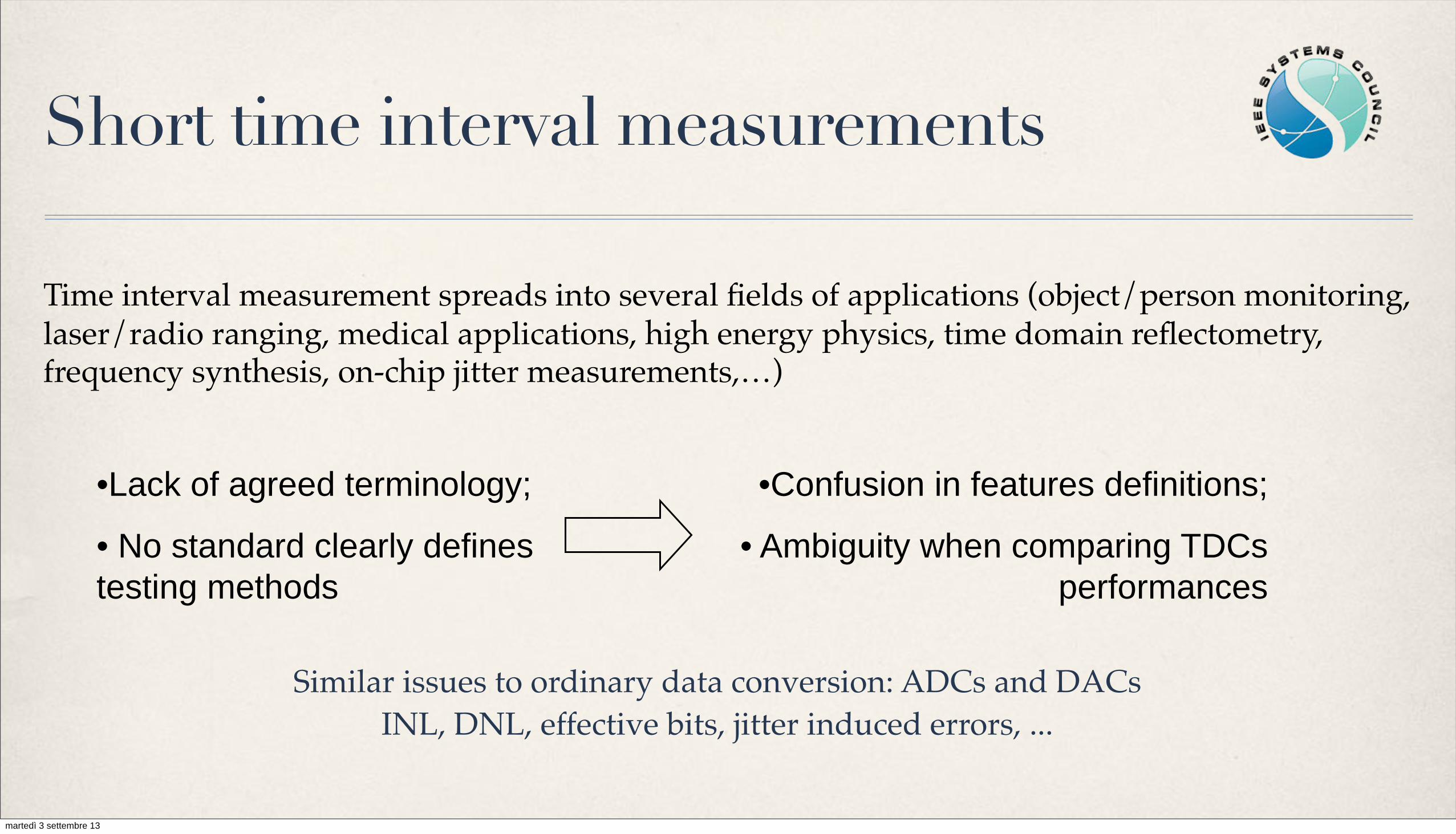
Short time interval measurements
Time interval measurement spreads into several fields of applications (object/person monitoring, laser/radio ranging, medical applications, high energy physics, time domain reflectometry, frequency synthesis, on-chip jitter measurements,…)
• Lack of agreed terminology;
• No standard clearly defines testing methods
• Confusion in features definitions;
• Ambiguity when comparing TDCs performances
Similar issues to ordinary data conversion: ADCs and DACsINL, DNL, effective bits, jitter induced errors, ...
martedì 3 settembre 13
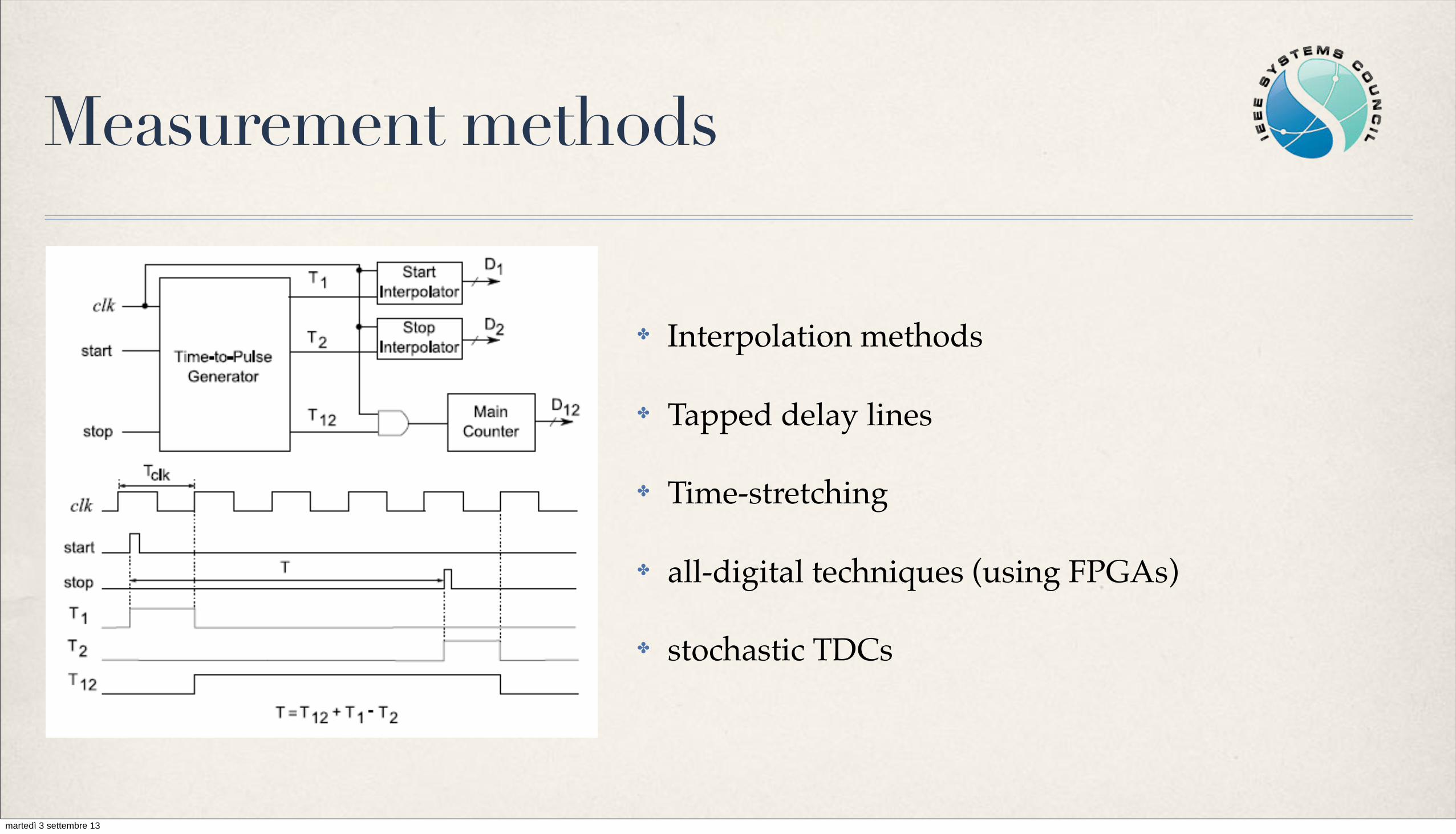
Measurement methods
✤ Interpolation methods
✤ Tapped delay lines
✤ Time-stretching
✤ all-digital techniques (using FPGAs)
✤ stochastic TDCs
martedì 3 settembre 13

Ongoing research on TDCs
mr: Measurement rate
Pd: Power consumption
A: Size
martedì 3 settembre 13

Research opportunities in the TDC area
✤ Characterization and testing methods
✤ New architectures (power consumption, sensitivity to environmental factors, ...)
✤ Applications: radar, all time-domain based sensing/measuring systems (more in coming slides)
✤ Our contributions in the area of modeling, VLSI design of a new architecture using pulse stretching and incremental sigma delta
martedì 3 settembre 13

Antennas
✤ 2 major realization: disc-cone - 1 GHz and planar - 5-6 GHz
martedì 3 settembre 13
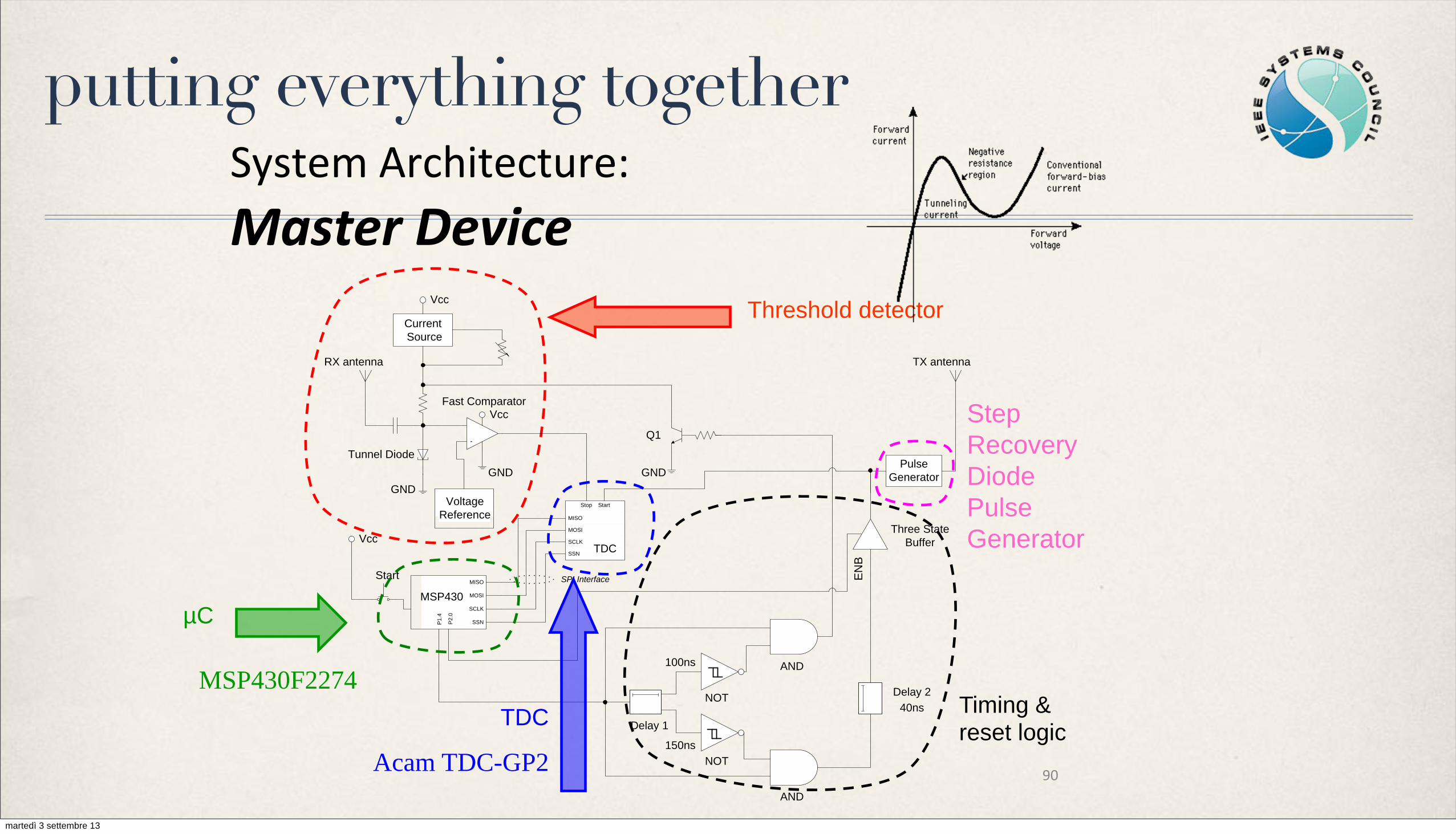
putting everything togetherSystem'Architecture:''Master'Device'
RX antenna TX antenna
Tunnel Diode
GND
Q1
GNDPulse
Generator
Current Source
Vcc
Fast Comparator
Voltage Reference
-
GND
Vcc
MISO
MOSI
SCLK
SSN
Stop Start
TDC
MISO
MOSI
SCLK
SSN
SPI Interface
MSP430
Vcc
P1.4
P2.
0
Start
NOT
Delay 1
AND
Three State Buffer
Delay 2
150ns
AND
100ns
NOT
40ns
EN
B
Threshold detector
µC
TDC
Acam TDC-GP2
Timing & reset logic
Step Recovery Diode Pulse Generator
MSP430F2274
90'
martedì 3 settembre 13

Ranging measurements
Dist:60-220 cm
Step: 20 cm
7500 RTT measurement results for each distance.
ns.std 30≅
Heteroscedastic system
martedì 3 settembre 13

Validation
Measured RTT
Mean and Mode values vs distance
Higher slope than ideal
martedì 3 settembre 13
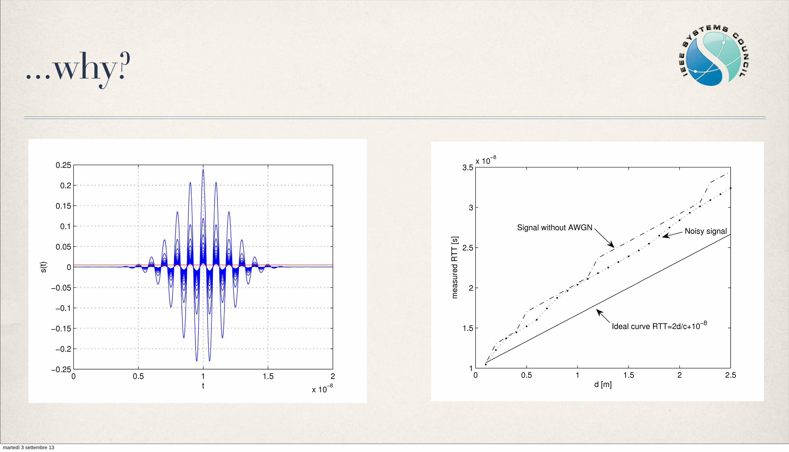
...why?
martedì 3 settembre 13

Ranging: experimental data
Experi-mental data
Correction factor
obtained by applying
linear regression
martedì 3 settembre 13
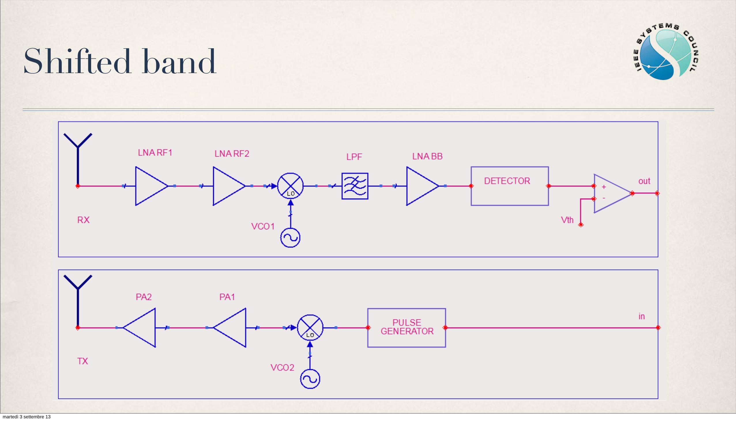
Shifted band
martedì 3 settembre 13

The realized instrumentSUBMITTED TO: IEEE TRANS. INSTR. AND MEAS., MAY 2012 3
arrival time. The comparator threshold can be set by meansof a suitable device pin which, in the present application, isdriven by the DCU. Clearly this setting allows trading receiversensitivity with error probability. The RTT measurement isfinally performed by the on–board TDC [32].
From the design point of view a special attention has beenpaid to power consumption minimization. Another importantsystem design objective was the determination of the right IFgain. This gain has been set to have the receiver noise floor (i.e.the front-end output power without input signal) at exactly thedetector threshold power PTH
D . This power is the minimuminput power required by the detector to overcome its internalnoise and is equal to about !20 dBm. The overall receivergain GRX has thus been set to:
GRX =PTHD
k T0 FR BBPF" 52dB (1)
where k is the Boltzmann constant, T0 = 290K is the IEEEstandard temperature, FR is the receiver noise figure andBBPF is the equivalent noise bandwidth of the band–pass fil-ter. Using simple assumptions we estimated FR # 3.5 dB andBBPF # 800MHz. The IF gain GIF can thus immediatelybe derived as:
GIF =GRX
GLNA GM1 GBPF" 35dB (2)
where GLNA, GM1 , GBPF are the low–noise–amplifier, mixerM1 and band–pass–filter gains, respectively. The resultingUWB receiver sensitivity amounts to !61 dBm.
The realized prototype is shown in Fig. 3. It is made ona low–cost FR4 printed circuit board along with microstripinterconnection technology. The overall components cost isestimated to be around $50 (year 2012) and can further bereduced by properly engineering the circuit. The overall powerconsumption is about 2.5W at 5V supply, mainly due tothe power amplifiers. Devices made commercially availableafter the end of this research already require less power, whilekeeping the same electrical parameters.
The measured transmitted pulse is shown in Fig. 4. Mea-surement results have been obtained using an equivalent–time numerical sampling oscilloscope with 20 GHz analogbandwidth and 10 Msample/s sampling rate. Consequently, thesignal envelope in Fig. 4 is more significant than fine details.While Fig. 4(A) shows the pulse generated in the baseband,in Fig. 4(B) measurement results are shown after modulationwith the 5.6 GHz sinusoidal source, using a fixed 10 dBattenuator. This latter figure shows that the attenuated peak–to–peak value is equal to 530mV and that a good suppressionof the carrier is obtained when the pulse generator is off (i.e.90mV residual amplitude). To appreciate the pulse frequencycontent, spectra are graphed in Fig. 5. Data have obtainedusing a 20dB attenuator and show the baseband and band-shifted behavior of the generated pulse. The carrier is clearlyseen around 5.6 GHz. By following the approach taken in [33],the single–shot spatial resolution, dr, can be estimated usingthe expression:
dr = ctR0.7
" 12.8cm
Fig. 3. Fabricated UWB transceiver proptotype operating at 5.6GHz. (A)Receiver, (B) Transmitter.
where c is the speed–of–light in vacuum and tR " 0.3 ns isthe main pulse rise–time. Thus, as per this design, a single–shot resolution of about 13 cm is achieved and a much betterfigure is expected when measurement results are averaged, asshown in sec. IV.
0 0.5 1 1.5 2 2.5 3 3.5 4 4.5 5 5.5 6 6.5 7 7.5−0.05
0
0.05
0.1
0.15
0.2
0.25
0.3
0.35
0.4
time (ns)
ampl
itude
(V) (A)
0 0.5 1 1.5 2 2.5 3 3.5 4 4.5 5
−0.25
−0.2
−0.15
−0.1
−0.05
0
0.05
0.1
0.15
0.2
0.25
time (ns)
ampl
itude
(V) (B)
Fig. 4. UWB pulse measurements obtained using a sampling oscilloscopewith 20 GHz analog bandwidth, 10 MSample/s sampling rate. (A) Basebandgenerated UWB pulse (20 dB attenuator inserted).; (B) 5.6 GHz modulatedpulse with peak–to–peak value 530mV and rise–time about equal to 0.3 ns(10 dB attenuator inserted).
SUBMITTED TO: IEEE TRANS. INSTR. AND MEAS., MAY 2012 4
0 0.2 0.4 0.6 0.8 1 1.2 1.4 1.6 1.8 2x 10⁹
−80
−70
−60
−50
−40
−30
−20
Hz
dBm
(A)
4 4.5 5 5.5 6 6.5 7x 10⁹
−80
−70
−60
−50
−40
−30
−20
Hz
dBm
(B)
Fig. 5. UWB pulse spectral measurements results. (A) Baseband generatedUWB pulse; (B) 5.6 GHz modulated pulse (20 dB attenuator inserted).
B. Design of the Antenna
The antenna design guideline was the good matching in thesignal band and a proper antenna radiation pattern. This latterparameter is of great importance, since anisotropy in emittedpower results in modifications of RTT by the radio–frequencydetector, beyond what can be recovered using system cali-bration. We choose an ultra–wideband monopole in order toachieve a compact size and omnidirectional behavior in theazimuthal plane (i.e. around the antenna vertical axes). Thereare many different UWB monopole antennas in literature,one of the most known being that introduced in [34]. It iscomposed of a circular printed disk fed directly by a microstripline. A scheme of the antenna layout is shown in Fig. 6.This design is a modification of the conventional circular diskmonopole, obtained by adding a via hole that allows a bettermatching of the antenna [35]. The antenna has been designedwith a disc diameter of 12 mm, D = 1.4 mm and G = 0.2mm on FR4 substrate 1.6 mm thick. Fig. 6 shows the antennaschematic and assembly, including the SubMiniatur version–A (SMA) connector, and figure Fig. 7 shows the measuredreflection coefficient at the SMA port, that confirms the goodmatching in the 5–7 GHz band and a bandwidth in excess of2 GHz. Measurement results shown in Fig. 7 have been takenusing a network analyzer with 10MHz – 40 GHz bandwidth,previously calibrated for measuring the S11 parameter [36].
III. POSITION ESTIMATION
Localization on a plane based on RTT requires distancemeasurements from 3 slaves of known position. When thecommunication channel is noiseless the RTT characterizingthe communication between the master and the i-th slave canbe approximately modeled as:
ti =2!iv
+ "i i = 1, 2, 3 (3)
where !i is the unknown distance between the master and i-th slave, v is the pulse apparent speed, keeping into accountboth propagation delay and distance dependent contributions
Fig. 6. The UWB antenna layout scheme (left) and its actual implementation(right). The detail of the gap G is enlarged in the inset.
Fig. 7. Measured reflection coefficient (S11) of the antenna.
to the detection latency, assumed linear [21]. Moreover "i isthe delay introduced by the hardware needed to receive andecho this pulse in the i-th slave and to transmit and receivethe pulse on the master’s side. Accordingly, since it dependson device tolerances and environmental factors, the DCU isdesigned so to minimize the number of components in thesignal path. Equation (3) can be inverted to obtain !i from ameasurement of ti, as follows:
!i =v
2(ti ! "i) i = 1, 2, 3 (4)
that outlines a linear relationship between RTT and distancemeasurement, in which v and "i are unknowns for a givenmeasurement setup. To estimate these values calibration is per-formed beforehand, by putting the master at known distancesfrom the i-th slave and by measuring the corresponding valuesof ti [37]. Outcomes in the calibration of the 3 slaves in oursystem are shown in Fig. 8. Data are obtained by moving theslaves on a linear trajectory with respect to the master putat a fixed distance and by recording the corresponding RTTs.Linear fitting is finally performed. Even though calibrationis performed along one direction only, accuracy performanceis not degraded as it will be shown in section IV. It can beobserved that the RTTs increase approximately linearly in theconsidered range with slopes and intercepts displayed in Tab. I.These values have been obtained by using the three slavedevices and by averaging N = 5 · 103 measurement results
SUBMITTED TO: IEEE TRANS. INSTR. AND MEAS., MAY 2012 3
arrival time. The comparator threshold can be set by meansof a suitable device pin which, in the present application, isdriven by the DCU. Clearly this setting allows trading receiversensitivity with error probability. The RTT measurement isfinally performed by the on–board TDC [32].
From the design point of view a special attention has beenpaid to power consumption minimization. Another importantsystem design objective was the determination of the right IFgain. This gain has been set to have the receiver noise floor (i.e.the front-end output power without input signal) at exactly thedetector threshold power PTH
D . This power is the minimuminput power required by the detector to overcome its internalnoise and is equal to about !20 dBm. The overall receivergain GRX has thus been set to:
GRX =PTHD
k T0 FR BBPF" 52dB (1)
where k is the Boltzmann constant, T0 = 290K is the IEEEstandard temperature, FR is the receiver noise figure andBBPF is the equivalent noise bandwidth of the band–pass fil-ter. Using simple assumptions we estimated FR # 3.5 dB andBBPF # 800MHz. The IF gain GIF can thus immediatelybe derived as:
GIF =GRX
GLNA GM1 GBPF" 35dB (2)
where GLNA, GM1 , GBPF are the low–noise–amplifier, mixerM1 and band–pass–filter gains, respectively. The resultingUWB receiver sensitivity amounts to !61 dBm.
The realized prototype is shown in Fig. 3. It is made ona low–cost FR4 printed circuit board along with microstripinterconnection technology. The overall components cost isestimated to be around $50 (year 2012) and can further bereduced by properly engineering the circuit. The overall powerconsumption is about 2.5W at 5V supply, mainly due tothe power amplifiers. Devices made commercially availableafter the end of this research already require less power, whilekeeping the same electrical parameters.
The measured transmitted pulse is shown in Fig. 4. Mea-surement results have been obtained using an equivalent–time numerical sampling oscilloscope with 20 GHz analogbandwidth and 10 Msample/s sampling rate. Consequently, thesignal envelope in Fig. 4 is more significant than fine details.While Fig. 4(A) shows the pulse generated in the baseband,in Fig. 4(B) measurement results are shown after modulationwith the 5.6 GHz sinusoidal source, using a fixed 10 dBattenuator. This latter figure shows that the attenuated peak–to–peak value is equal to 530mV and that a good suppressionof the carrier is obtained when the pulse generator is off (i.e.90mV residual amplitude). To appreciate the pulse frequencycontent, spectra are graphed in Fig. 5. Data have obtainedusing a 20dB attenuator and show the baseband and band-shifted behavior of the generated pulse. The carrier is clearlyseen around 5.6 GHz. By following the approach taken in [33],the single–shot spatial resolution, dr, can be estimated usingthe expression:
dr = ctR0.7
" 12.8cm
Fig. 3. Fabricated UWB transceiver proptotype operating at 5.6GHz. (A)Receiver, (B) Transmitter.
where c is the speed–of–light in vacuum and tR " 0.3 ns isthe main pulse rise–time. Thus, as per this design, a single–shot resolution of about 13 cm is achieved and a much betterfigure is expected when measurement results are averaged, asshown in sec. IV.
0 0.5 1 1.5 2 2.5 3 3.5 4 4.5 5 5.5 6 6.5 7 7.5−0.05
0
0.05
0.1
0.15
0.2
0.25
0.3
0.35
0.4
time (ns)
ampl
itude
(V) (A)
0 0.5 1 1.5 2 2.5 3 3.5 4 4.5 5
−0.25
−0.2
−0.15
−0.1
−0.05
0
0.05
0.1
0.15
0.2
0.25
time (ns)
ampl
itude
(V) (B)
Fig. 4. UWB pulse measurements obtained using a sampling oscilloscopewith 20 GHz analog bandwidth, 10 MSample/s sampling rate. (A) Basebandgenerated UWB pulse (20 dB attenuator inserted).; (B) 5.6 GHz modulatedpulse with peak–to–peak value 530mV and rise–time about equal to 0.3 ns(10 dB attenuator inserted).
SUBMITTED TO: IEEE TRANS. INSTR. AND MEAS., MAY 2012 4
0 0.2 0.4 0.6 0.8 1 1.2 1.4 1.6 1.8 2x 10⁹
−80
−70
−60
−50
−40
−30
−20
Hz
dBm
(A)
4 4.5 5 5.5 6 6.5 7x 10⁹
−80
−70
−60
−50
−40
−30
−20
Hz
dBm
(B)
Fig. 5. UWB pulse spectral measurements results. (A) Baseband generatedUWB pulse; (B) 5.6 GHz modulated pulse (20 dB attenuator inserted).
B. Design of the Antenna
The antenna design guideline was the good matching in thesignal band and a proper antenna radiation pattern. This latterparameter is of great importance, since anisotropy in emittedpower results in modifications of RTT by the radio–frequencydetector, beyond what can be recovered using system cali-bration. We choose an ultra–wideband monopole in order toachieve a compact size and omnidirectional behavior in theazimuthal plane (i.e. around the antenna vertical axes). Thereare many different UWB monopole antennas in literature,one of the most known being that introduced in [34]. It iscomposed of a circular printed disk fed directly by a microstripline. A scheme of the antenna layout is shown in Fig. 6.This design is a modification of the conventional circular diskmonopole, obtained by adding a via hole that allows a bettermatching of the antenna [35]. The antenna has been designedwith a disc diameter of 12 mm, D = 1.4 mm and G = 0.2mm on FR4 substrate 1.6 mm thick. Fig. 6 shows the antennaschematic and assembly, including the SubMiniatur version–A (SMA) connector, and figure Fig. 7 shows the measuredreflection coefficient at the SMA port, that confirms the goodmatching in the 5–7 GHz band and a bandwidth in excess of2 GHz. Measurement results shown in Fig. 7 have been takenusing a network analyzer with 10MHz – 40 GHz bandwidth,previously calibrated for measuring the S11 parameter [36].
III. POSITION ESTIMATION
Localization on a plane based on RTT requires distancemeasurements from 3 slaves of known position. When thecommunication channel is noiseless the RTT characterizingthe communication between the master and the i-th slave canbe approximately modeled as:
ti =2!iv
+ "i i = 1, 2, 3 (3)
where !i is the unknown distance between the master and i-th slave, v is the pulse apparent speed, keeping into accountboth propagation delay and distance dependent contributions
Fig. 6. The UWB antenna layout scheme (left) and its actual implementation(right). The detail of the gap G is enlarged in the inset.
Fig. 7. Measured reflection coefficient (S11) of the antenna.
to the detection latency, assumed linear [21]. Moreover "i isthe delay introduced by the hardware needed to receive andecho this pulse in the i-th slave and to transmit and receivethe pulse on the master’s side. Accordingly, since it dependson device tolerances and environmental factors, the DCU isdesigned so to minimize the number of components in thesignal path. Equation (3) can be inverted to obtain !i from ameasurement of ti, as follows:
!i =v
2(ti ! "i) i = 1, 2, 3 (4)
that outlines a linear relationship between RTT and distancemeasurement, in which v and "i are unknowns for a givenmeasurement setup. To estimate these values calibration is per-formed beforehand, by putting the master at known distancesfrom the i-th slave and by measuring the corresponding valuesof ti [37]. Outcomes in the calibration of the 3 slaves in oursystem are shown in Fig. 8. Data are obtained by moving theslaves on a linear trajectory with respect to the master putat a fixed distance and by recording the corresponding RTTs.Linear fitting is finally performed. Even though calibrationis performed along one direction only, accuracy performanceis not degraded as it will be shown in section IV. It can beobserved that the RTTs increase approximately linearly in theconsidered range with slopes and intercepts displayed in Tab. I.These values have been obtained by using the three slavedevices and by averaging N = 5 · 103 measurement results
martedì 3 settembre 13
Experimental characterization
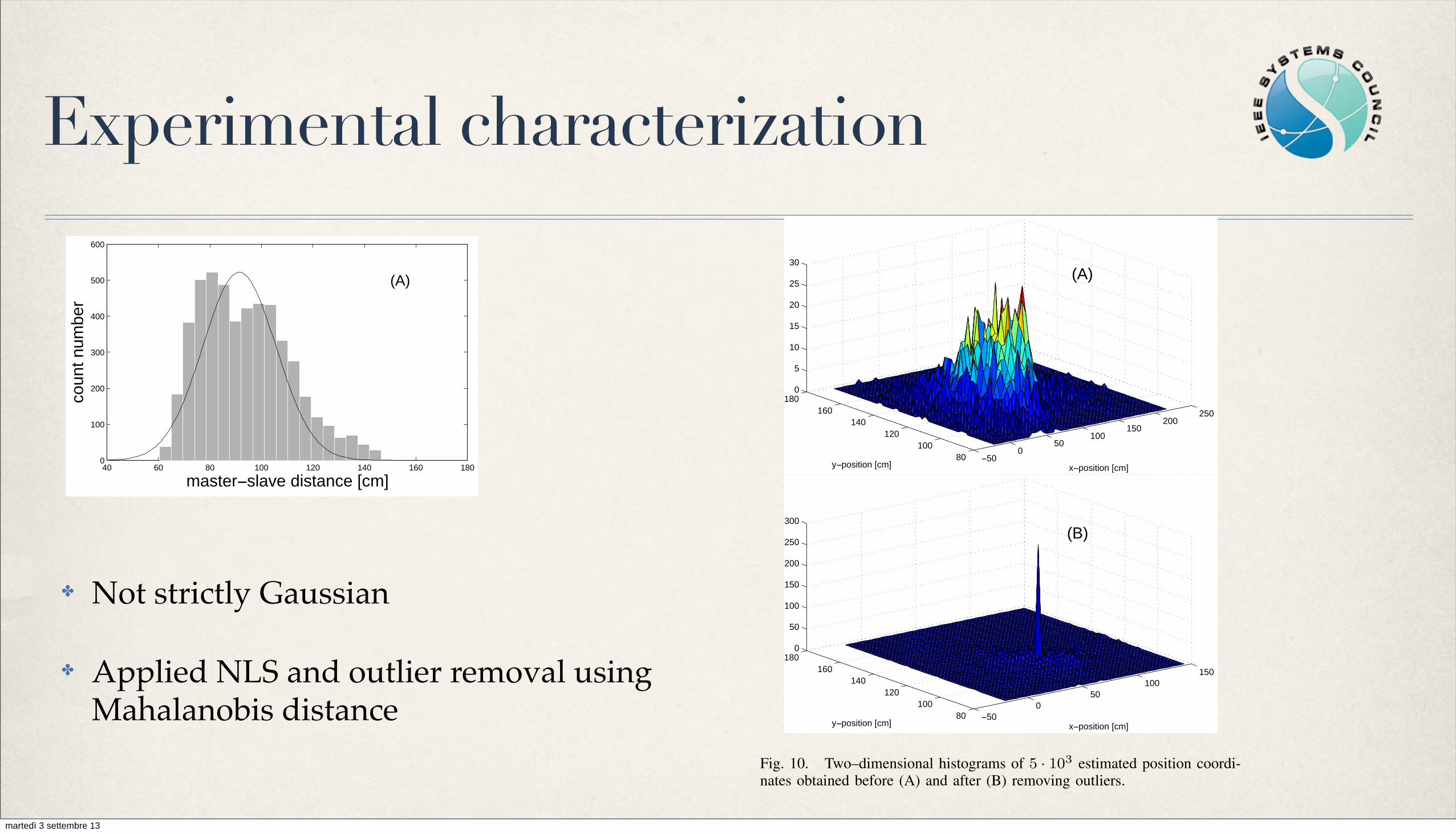
✤ Not strictly Gaussian
✤ Applied NLS and outlier removal using Mahalanobis distance
SUBMITTED TO: IEEE TRANS. INSTR. AND MEAS., MAY 2012 6
estimated in sec. III using information on pulse rise–time.While the resulting estimated PDF is still asymmetric aroundthe mean, the outlier removal algorithm reduces its skewnessand mitigates the effect of markedly uninformative pulses.Moreover, experiments have highlighted heteroscedasticity inthe collected RTTs records, the variance being distance–dependent. This results in worse estimation accuracy at largerdistances from slaves, but could be exploited to improve accu-racy of used position estimation algorithms by including thisinformation in the procedure’s constraints. Thus, the overallestimation procedure is based on four steps: compensation ofoffset and slope by means of each node calibration curve,removal of outliers, averaging of N measurement results andapplication of the NLS algorithm. Similary to the approachtaken in [39], Tab. II reports calculations regarding the algo-rithm computational complexity for a generic setup in whichthe three spatial coordinates are estimated, by using S slavesand N measurement results for each slave.
20 40 60 80 100 120 140 160 180845
850
855
860
865
870
875
880
distance [cm]
RTT
[ns]
slave 1slave 2slave 3
Fig. 8. RTTs of the 3 slaves used in the system under calibration conditionsincluding the corresponding linear fitting.
IV. POSITION MEASUREMENT RESULTS
The measurement setup includes 3 slaves put at known posi-tions at the vertices of a triangle in a laboratory environment,as shown in Fig. 11. The master has been navigated on arectangular path and 8 fixed positions have been estimatedon the basis of records having size N = 5 · 103. For eachentry in the record, 3 RTTs have been measured by the TDC,managed by the DCU. Compensation of slope and interceptusing calibration data has been applied and outliers removedand substituted by the mean in each record. The effects ofthe outlier removal procedure are shown in Fig. 10 wherethe position histograms have been plotted before and afterremoval obtained using data in one of the records. Finally, thethree mean values obtained using N–size records modifiedaccording to the described outlier removal technique, havebeen used as the known data for the NLS algorithm toprovide position estimations, shown in Fig. 11 using circles.Experimental data show that good matching between knownand estimated positions has been achieved, while type–A stan-dard uncertainty [40] in short–distance single measurement
40 60 80 100 120 140 160 1800
100
200
300
400
500
600
(A)
master−slave distance [cm]
coun
t num
ber
40 60 80 100 120 140 160 1800
100
200
300
400
500
600
(B)
master−slave distance [cm]
coun
t num
ber
Fig. 9. Histograms of 5 · 103 RTTs in a given master–slave configuration,before (A) and after (B) removing outliers. Gaussian fits are shown forreference purposes.
results did not exceed 10 cm, after outlier removal. Thisresult is consistent with the value of the pulse rise–time andcomparable with those obtained by other researchers usingmore complex architectures [15].
V. ANALYSIS OF UNCERTAINTY SOURCES
In this section, we analyze the effects of system nonidealities to the uncertainty in the estimation of the masterposition. Since start and stop triggers originate when the pulsecrosses a fixed–value threshold, the shape of the transmittedand received pulses plays a major role in influencing systemaccuracy and is the dominant source of uncertainty in thisrealization. The pulse shape is in turn largely dependent onthe characteristics of the pulse generator, on the amount ofwideband noise, on multipath induced effects, on path–lossesand on deviations and tolerances in the fixed frequenciesused to drive the mixer. The high–slew rate properties ofthe UWB pulse, make it rather robust against time–localdisturbances, but its time–dependent derivative is the mainreason for the measured RTTs not to exhibit a symmetricdistribution. In fact, wideband noise superimposed on the pulsesignal, makes the probabilities of being above or below theset threshold asymmetric. As a consequence, the estimator ofthe RTT probability density function applied to experimentaldata obtained at several master–slaves distances confirm theleptokurtic behavior of the RTTs distributions.
Multipath effects play also a role, both in determining thepulse shape and in influencing RTT measurements. It is oftenargued that UWB–based transmission is resilient to multipath
SUBMITTED TO: IEEE TRANS. INSTR. AND MEAS., MAY 2012 7
TABLE IICOMPUTATIONAL COMPLEXITY OF THE POSITION ESTIMATION ALGORITHM.
Multiplications/divisions Additions/subtractions Sorting operations Transpose operations Inverse operationsCalibration N ! S N ! S - - -Outlier rejection N ! S N ! S S - -Data averaging S (N " 1)! S - - -LS 21S 6(3S " 2) - [ ]S!3 [ ]3!3
NLSThe NLS algorithm is first based on a Jacobian operation to linearize the nonlinear position equations. Then theLS equations can be used to estimate the position. Therefore, the computational complexity of NLS is as follows:# NLS cycles ! (computational complexity of LS + Jacobian operation).
N=number of measurement results for each slave, S=number of slaves.
−500
50100
150200
250
80100
120140
160180
0
5
10
15
20
25
30(A)
x−position [cm]y−position [cm]
−500
50100
150
80100
120140
160180
0
50
100
150
200
250
300
x−position [cm]
(B)
y−position [cm]
Fig. 10. Two–dimensional histograms of 5 · 103 estimated position coordi-nates obtained before (A) and after (B) removing outliers.
effects. Of course, reflected RF pulses arrive at a later time atthe receiver with respect to the line–of–sight pulse, so thattheir contribution might seem uninfluencial in determiningthe RTT. However, closely time–spaced replica of the pulseat the receiver, that may happen in a laboratory setup, maymodify the shape and slopes in the received signal and thusinfluence measurement results. In order to verify this hypoth-esis, experimental data have also been collected in a semi–anechoic chamber, where multipath phenomena can largely beneglected. The demodulated pulses show markedly differentbehaviors. When reflections are not permitted, the pulse is asmall–energy compact support waveform. On the contrary, inthe laboratory environment, reflections in the walls and otherartifacts result in a longer transient behavior of the pulse,that is also characterized by a larger energy content. In bothcases, repeatability of measurements is confirmed by similarvalues in RTT standard deviations, but different calibrationcurves apply because of different experimental conditions. At
0 20 40 60 80 100 120 140 160 180 200 2200
20
40
60
80
100
120
140
160
180
200
220
x−position [cm]
y−po
sitio
n [c
m]
Mean error 5.303 cm
slave 1slave 2slave 3Real pathEstimated path
Fig. 11. Final position estimation results: squares indicate the position ofthe slaves, black dots the nominal position of the master, circles the estimatedpositions of the master.
the same time, the laboratory setup guarantees an extendedrange of transmission over that obtained in the semi–anechoicchamber because of the wave–guide effect of walls and ofthe resulting constructive interference induced by multipath.Sample distributions of measured RTTs have been processedin both environments, exhibiting similar overall behaviors.However, since multipath is a highly position dependent phe-nomenon [41], its effects must be taken into consideration if anenvironmentally–independent positioning system is a designrequirement. Deviations in the initial phase and frequenciesused in the modulators and demodulators, to translate the pulsein the transmitters and receivers, reduces the received pulseamplitudes in the nodes and the related detection probability,with respect to what happens under ideal conditions. Finetuning or more involved hardware architectures could mitigatethe effects of this phenomenon at the expense of an increasedcomplexity. It is also to be observed that a missed pulse can bedetected by putting simple constraints on the RTT measuredby the TDCs, such as when detecting over–range events.
Wideband noise and path–loss effects contribute to bothreduce the SNR at the receiver side and to attenuate thereceived signal. As an overall result, an increased standarddeviation is expected at larger distances. This phenomenonis evidenced in Fig. 12, where estimated standard deviationsin RTTs is shown as a function of the master–slave distance
martedì 3 settembre 13

Positioning results: static
!
5000 records for each pointNLS - estimate
SUBMITTED TO: IEEE TRANS. INSTR. AND MEAS., MAY 2012 1
A 5.6 GHz UWB Position Measurement SystemAlessandro Cazzorla, Guido De Angelis, Senior Member, IEEE, Antonio Moschitta, Member, IEEE,
Marco Dionigi, Member, IEEE, Federico Alimenti, Senior Member, IEEE,and Paolo Carbone, Senior Member, IEEE
Abstract—This paper describes the design and realization ofa 5.6 GHz ultra–wide bandwidth based position measurementsystem. The system has been entirely made using off–the–shelf components and achieves centimeter level accuracy in anindoor environment. It is based on asynchronous modulated pulseround–trip–time measurements. Both system level and realizationdetails are described along with experimental results includingestimates of measurement uncertainties.
I. INTRODUCTION
THE topic of indoor positioning has gained increasinginterest over the years in the scientific literature because
of the involved technical challenges and of the demand in theapplication market. While it can be envisioned that portableelectronic devices will feature seamless outdoor/indoor posi-tioning capabilities in the future, current technology does notenable it yet at acceptable cost–performance trade–offs. Sev-eral approaches have been proposed over time that addressedthe positioning problem from various perspectives but, eventhough requests for applications are growing at a fast pace,technology still seems to lay behind. The interested reader ispointed to [1], in which an updated state–of–the art analysis onthe available techniques and their accuracy–vs–range figuresis published.
The main challenges in the radio indoor positioning fieldare the high accuracy level required by the majority ofthe applications and the features of the indoor propagationchannel [2], [3]. In this context, pulse–based Ultra–WideBand(UWB) systems are interesting, mainly due to the fine timeresolution provided by sub–nanosecond pulses [4]–[6]. Thisfeature enables a high level of accuracy in measuring distance,potentially in the centimeter order. Furthermore, it allows forrobustness to multipath phenomena which represent a majorchallenge of the indoor radio propagation channel [7]. Variousresearches consider UWB–based positioning, under differentviewpoints. These include channel modeling, estimation ofmultipath components and evaluation of the Cramer–RaoLower Bound on positioning accuracy, under given conditions[8]–[12].
While CMOS VLSI stands as an enabling technology toattack the positioning problem starting from basic buildingblocks [13], few complete realizations based on CommercialOff–The–Shelf (COTS) components are described in the liter-ature and even fewer do not use external high–end and stand–alone numerical instruments. This work describes results ob-
All authors are with the Department of Electrical and InformationEngineering, University of Perugia, Italy, PG, 06125 e-mail: [email protected]; {guido.deangelis; moschitta; dionigi; alimenti; [email protected].}
Manuscript sent May 31, 2011
tained with a positioning system entirely realized using COTScomponents to reduce complexity and implementation costs. Itproposes a simple architecture that extends the state–of–the–art in this field [14] by proving experimentally that accuratepositioning can be achieved by avoiding the need for complexand expensive solutions. In fact, recently published positioningmethods rely on the synchronization of anchors or on the usageof hybrid Direction of Arrival–Time of Arrival (DOA-TOA)approaches or on the usage of complex high speed correlatorsand digital processing, as published in [15]–[18]. At the sametime, because of the adopted measurement method and of thechosen frequency band, bulky antenna arrays as those used in[19] may be avoided. It is also worth noting that the proposedtechnique may be competitive, from an accuracy standpoint,with recently developed commercial solutions such as [20],that feature 15 cm ranging error standard deviation underoptimal conditions.
Experimental outcomes described in this paper are based ona previously developed ranging system described in [21]. Theonly common subsystem shared by the two implementations isthe Digital Control Unit (DCU), while transceivers includingantennas, have been re–designed to work at 5.6 GHz centerfrequency and new digital signal processing has been adoptedto improve position estimation capabilities. Localization isachieved by using Round–Trip–Time (RTT) measurementsbetween master and slave nodes, to further reduce complexityby avoiding the synchronization of anchors. Lack of syn-chronization requirements is traded–off in this case for thedetermination and compensation of latencies introduced by theresponder devices. This implies the need for system calibrationthat is not seen as an issue because of the possibility tolargely automate this process. Experimental results describedin section IV show that state–of–the–art accuracy can beachieved while keeping low circuital complexity.
II. SYSTEM DESIGN
The design of an UWB–based position measurement systemimplies competencies from many engineering fields, includ-ing metrology, radio–frequency, digital signal processing andsystem engineering, on the basis of a truly trans– and inter–disciplinary approach. The position measurement architecturedescribed in this paper is based on a network of transceivers,in which a master device is located by measuring the RTTfrom slave nodes located at known positions, as shown inFig. 1. Each node includes a DCU and a radio–frequency–transceiver. While each slave is designed so as to transmit apulse when it receives a pulse, with a possibly constant andsystematic delay, the master node also includes fine–resolution
Micro-displacements: achievable resolution below 1mm,
if several measurement results are averaged
martedì 3 settembre 13

Positioning results: dynamic / tracking
✤ Sensor fusion using Inertial Measurement Unit to compensate when static data are not available
'ZRGTKOGPVCN�4CFKQ�+PFQQT�2QUKVKQPKPI�5[UVGOU�$CUGF�QP�4QWPF�6TKR�6KOG�OGCUWTGOGPV ���
���������������������������������������������D��������������������������������������������������������������������������������������E��)LJ������+LJK�G\QDPLF�WHVWV���D��8:%�SRVLWLRQLQJ�VWDQG�DORQH��LW�FDQ�EH�QRWLFHG�WKDW�RYHUVKRRW�LV�SUHVHQW�� DQG� SRRU� WUDFNLQJ� SHUIRUPDQFH� LV� REVHUYHG�� �E�� LQIRUPDWLRQ� IXVLRQ� ZLWK� ,16�� QR�RYHUVKRRW�DQG�EHWWHU�WUDFNLQJ�SHUIRUPDQFH�KDV�EHHQ�REVHUYHG��'H�$QJHOLV�HW�DO�������E����7KH�ODVW�VHW�RI�WHVWV�FRQVLVWHG�LQ�KLJK�G\QDPLF�H[SHULPHQWV�LQYROYLQJ�WKH�FRPSOHWH�V\VWHP��LQFOXGLQJ� WKH� ,16� DQG� LQIRUPDWLRQ� IXVLRQ� SODWIRUP�� 7KH� H[SHULPHQW�ZDV� H[HFXWHG� RQ� WKH�VDPH�WUDMHFWRU\�DV�WKDW�RI�WKH�SUHYLRXV�VHW��EXW�LQ�WKLV�FDVH�WKH�PDVWHU�ZDV�PRYHG�TXLFNO\��DW�DSSUR[LPDWHO\� ��P�V�� ,QLWLDOO\� WKH� WHVW�ZDV�SHUIRUPHG�XVLQJ� WKH�8:%� V\VWHP�DORQH��7KLV�WHVW� DOORZHG� WR� GHPRQVWUDWH� VRPH� RI� WKH� OLPLWV� RI� WKH� 8:%� VWDQG�DORQH� V\VWHP�� PDLQO\�FDXVHG� E\� WKH� VORZ� XSGDWH� UDWH�� DV� VKRZQ� E\� WKH� RYHUVKRRW� � DQG� E\� WKH� ORZ� WUDFNLQJ�SHUIRUPDQFH� LQ� )LJ����D�� 6XEVHTXHQWO\�� DQRWKHU� WHVW� XVLQJ� WKH� IXOO� V\VWHP� ZLWK� ,16�PHDVXUHPHQW� LQWHJUDWLRQ�ZDV�H[HFXWHG�LQ�WKH�VDPH�H[SHULPHQWDO�FRQGLWLRQV��7KH�UHVXOWLQJ�GDWD� LV� VKRZQ� LQ� )LJ����E�� GHPRQVWUDWLQJ� WKH� FRQVLGHUDEOH� SHUIRUPDQFH� LPSURYHPHQW�REWDLQHG�� ,Q�SDUWLFXODU�� WKH� WUDMHFWRU\�RYHUVKRRW�KDV�EHHQ�HOLPLQDWHG�DQG�DQ�RYHUDOO� EHWWHU�WUDFNLQJ�EHKDYLRXU�FDQ�EH�REVHUYHG���
�����(WVWTG�FGXGNQROGPVU�����ȱ ��ȱ ���ȱ ��������ȱ ����������ȱ �¡������ȱ ��ȱ ���ȱ ������ȱ �������ȱ ���ȱ �����������ȱ ��ȱ ���ȱ���� ���ȱ �������ȱ ��������ȱ �����£��ȱ ��ȱ ���ǯȱ ��ȱ ����������ǰȱ �ȱ ������������ȱ ��ȱ ���ȱ ��������ȱ�����ȱ���������ȱ��ȱ��������¢ȱ�����ȱ�������ǰȱ ���ȱ���ȱ����ȱ��ȱ�����£���ȱ�ȱ�¢����ȱ ����ȱ��ȱ����¢ȱ���������ȱ ���ȱ����ȱ ���ȱ �������ȱ��������ȱ ���ȱ���ȱ �����������ǯȱ���ȱ ����ȱ �������¢ȱ�����ȱ���������ȱ���������ȱ��ȱ�������ȱřǯŗǰȱ��ȱ����ǰȱ��������ȱ��ȱ������ȱ��������ȱ������¢ȱ����ȱ��ȱ���śŖŖȱ�£ǯȱ�¢ȱ�����ȱ��ȱ �ȱ�����ȱ ���������Ȭ����������ȱ��������ǰȱ ��ȱ ��ȱ��������ȱ ��ȱ �����ȱ ����ȱ��������ȱ������ȱ���ȱ��������¢ȱ��ȱ�ȱ�������ȱ������ȱ��ȱ���ȱŜȱ£ȱ������ǰȱ���������ȱ���������ȱ������ȱ ȱ ���ȱ ���ȱ ����������ȱ �����ȱ ��� �ȱ ��ȱ ���ǯȱŗǯȱ �����������ǰȱ ����ȱ �ȱ ��������ȱ �����ȱ����������¢ȱ������ȱ��������ȱ����������ȱ ���ȱ���ȱ������������ȱ����ȱ�����ȱ�����ȱ�¢�����ǰȱ�����ȱWKHUH�LV�D�ORZHU�QXPEHU�RI�QDUURZEDQG�XVHUV�LQ�WKH���*+]�EDQG��2WKHU�IXWXUH�GHYHORSPHQWV�DUH�DLPHG�DW�LQFUHDVLQJ�WKH�FRPPXQLFDWLRQ�UDQJH��FRYHUDJH�DQG�XSGDWH�UDWH�RI�WKH�V\VWHP��DOVR� FRQVLGHULQJ� DGYDQFHV� LQ� WKH� LQIRUPDWLRQ� IXVLRQ� WHFKQLTXH� DQG� VLJQDO� SURFHVVLQJ�DOJRULWKPV�ȱ
��
'ZRGTKOGPVCN�4CFKQ�+PFQQT�2QUKVKQPKPI�5[UVGOU�$CUGF�QP�4QWPF�6TKR�6KOG�OGCUWTGOGPV ���
'ZRGTKOGPVCN�4CFKQ� +PFQQT�2QUKVKQPKPI�5[UVGOU�$CUGF�QP�4QWPF�6TKR�6KOG�OGCUWTGOGPV
#NGUUKQ�&G�#PIGNKU��#PVQPKQ�/QUEJKVVC��2GVGT�*¼PFGN�CPF�2CQNQ�%CTDQPG
:��'ZRGTKOGPVCN�4CFKQ�+PFQQT�2QUKVKQPKPI�5[UVGOU�
$CUGF�QP�4QWPF�6TKR�6KOG�/GCUWTGOGPV��
$OHVVLR�'H�$QJHOLV���$QWRQLR�0RVFKLWWD���3HWHU�+lQGHO��DQG�3DROR�&DUERQH���'HSDUWPHQW�RI�(OHFWURQLF�DQG�,QIRUPDWLRQ�(QJLQHHULQJ��',(,���8QLYHUVLW\�RI�3HUXJLD��
,WDO\��6LJQDO�3URFHVVLQJ�/DE��$&&(66�/LQQDHXV�&HQWUH��5R\DO�,QVWLWXWH�RI�7HFKQRORJ\��
6WRFNKROP��6ZHGHQȱ
����+PVTQFWEVKQP��
7KLV� FKDSWHU� SUHVHQWV� WKH� GHVLJQ� LVVXHV� DQG� SHUIRUPDQFH� FKDUDFWHUL]DWLRQ� UHVXOWV� RI� WZR�H[SHULPHQWDO�V\VWHPV�IRU�UDGLR�GLVWDQFH�PHDVXUHPHQW�DQG�SRVLWLRQLQJ��7KH�PDLQ�HQYLVLRQHG�DSSOLFDWLRQ� DUHD� IRU� WKHVH� V\VWHPV� LV� WKH� LQGRRU� HQYLURQPHQW�� FKDUDFWHUL]HG� E\� DQ�LQVXIILFLHQW� FRYHUDJH� RI� JOREDO� QDYLJDWLRQ� VDWHOOLWH� V\VWHPV� DQG� E\� LVVXHV� UHODWHG� WR� WKH�LQGRRU�UDGLR�SURSDJDWLRQ�FKDQQHO��,Q�SDUWLFXODU��VXFK�LVVXHV�LQFOXGH�PXOWLSDWK�SURSDJDWLRQ�DQG� WKH� DEVHQFH� RI� OLQH�RI�VLJKW�� )XUWKHUPRUH�� WKH� DSSOLFDWLRQV� IRU� LQGRRU� SRVLWLRQLQJ�V\VWHPV�XVXDOO\�UHTXLUH�D�KLJK�GHJUHH�RI�DFFXUDF\��ZKLFK�FDQ�EH�RI�WKH�RUGHU�RI�D�FHQWLPHWUH��LQ� WKH�SRVLWLRQ� HVWLPDWLRQ��5HFHQWO\�� WKLV� UHVHDUFK� DUHD� H[SHULHQFHG� D� FRQVLGHUDEOH� JURZWK�DQG�WKH�VWDWH�RI�WKH�DUW�LV�FKDUDFWHUL]HG�E\�D�ZLGH�DUUD\�RI�VROXWLRQV���,Q� WKLV� FRQWH[W�� WKH� V\VWHPV� GHVFULEHG� LQ� WKH� SUHVHQW� FKDSWHU� DUH� EDVHG� RQ� WZR� GLIIHUHQW�DSSURDFKHV�� DQ� 8OWUD�:LGHEDQG� �8:%�� SXOVH�EDVHG� VROXWLRQ� �'H�$QJHOLV� HW� DO��� ����D����'H�$QJHOLV� HW� DO��� ����D��� �'H� $QJHOLV� HW� DO��� ����F�� DQG� D� SODWIRUP� GHYHORSHG� XVLQJ�FRPPHUFLDO�GHYLFHV�FRPSO\LQJ�ZLWK�WKH�=LJ%HH�VWDQGDUG��6DQWLQHOOL�HW�DO����������+RZHYHU��ERWK�DSSURDFKHV�VKDUH�WKH�VDPH�SULQFLSOH�RI�RSHUDWLRQ��WKH�PHDVXUHPHQW�RI�VLJQDO�7LPH�2I�)OLJKW�� ,Q� SDUWLFXODU�� WKH� V\VWHPV� DUH� FDSDEOH� RI� PHDVXULQJ� WKH� 5RXQG�7ULS�7LPH� �577���HOLPLQDWLQJ� WKH�QHHG� IRU�DFFXUDWH�V\QFKURQL]DWLRQ�EHWZHHQ� WUDQVPLWWHUV�DQG�UHFHLYHUV��7KH�WLPH�LQWHUYDO�PHDVXUHPHQW�IXQFWLRQ�LV�SHUIRUPHG�LQ�ERWK�V\VWHPV�E\�D�FRPPHUFLDO�7LPH�WR�'LJLWDO�&RQYHUWHU��7'&��ZLWK����SV�UPV�UHVROXWLRQ��7KH�ILUVW�DSSURDFK�LQYROYHV�WKH�FRPSOHWH�GHVLJQ�SURFHVV�RI�WKH�SXOVH�8:%�UDGLR�LQWHUIDFH��WKDW�LV�WKH�FLUFXLWU\�QHFHVVDU\�WR�SURSHUO\�JHQHUDWH�DQG�GHWHFW�D�VXE�QDQRVHFRQG�SXOVH��7KHVH�EORFNV� KDYH� EHHQ� GHVLJQHG� DQG� EXLOW� IURP� VFUDWFK� XVLQJ� RII�WKH�VKHOI� FRPSRQHQWV� ZKHUH�SRVVLEOH��)XUWKHUPRUH��RWKHU� UHOHYDQW�EORFNV�DUH� WKH� WLPLQJ�DQG�FRQWURO� ORJLF�� WKH� LQWHUIDFH�ZLWK� WKH� 7'&� DQG� WKH� FRPPXQLFDWLRQ� ZLWK� D� 3&� IRU� GDWD� SURFHVVLQJ�� 7KH� RYHUDOO�DUFKLWHFWXUH� KDV� EHHQ� GHYHORSHG� XVLQJ� D� PDVWHU�VODYH� DSSURDFK�� LQ� ZKLFK� VHYHUDO� VODYHV��SXOVH� UHSHDWHUV�� DUH� SODFHG� LQ� IL[HG� DQG� NQRZQ� SRVLWLRQV� DQG� WKXV� FRQVWLWXWH� WKH�LQIUDVWUXFWXUH� RI� WKH� V\VWHP�� 7KH�PDVWHU� GHYLFH� LV� FDSDEOH� RI�PHDVXULQJ� LWV� GLVWDQFH�ZLWK�UHVSHFW�WR�WKH�VODYHV�DQG�RI�HVWLPDWLQJ�LWV�SRVLWLRQ�E\�PHDQV�RI�WULDQJXODWLRQ�DOJRULWKPV��$�
�
martedì 3 settembre 13
New directions
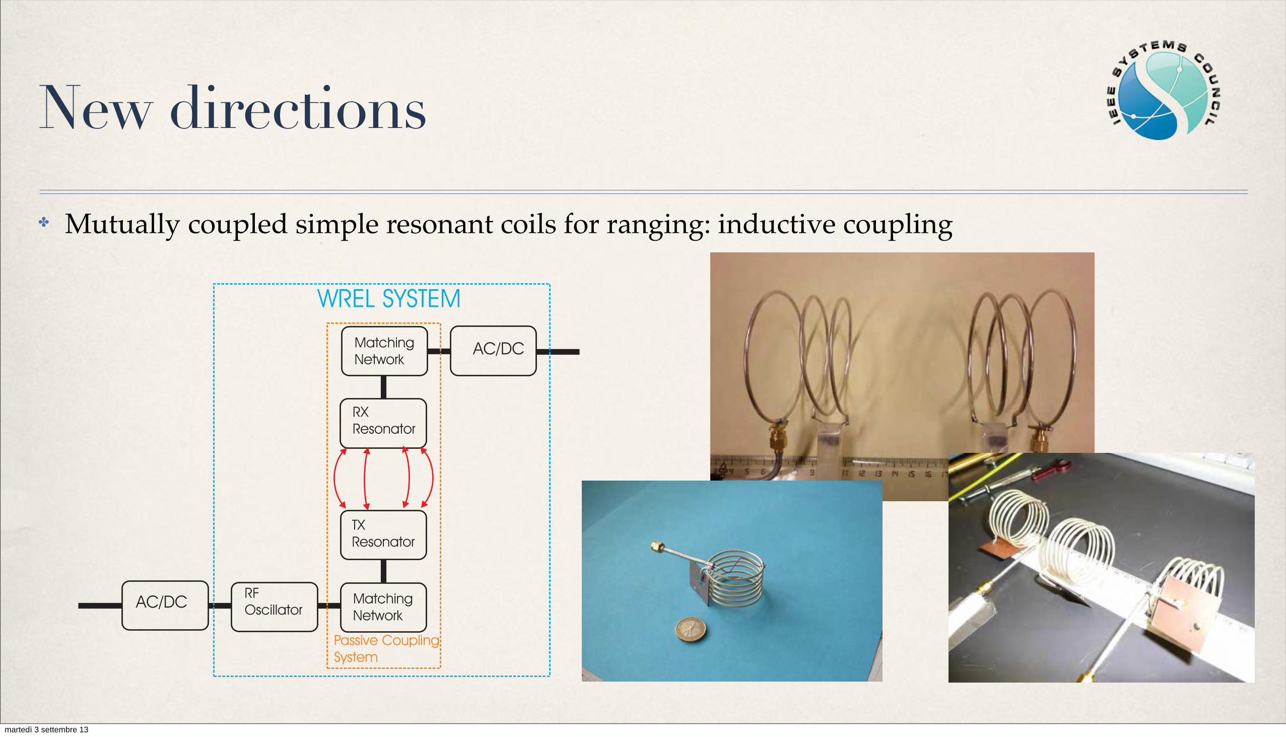
✤ Mutually coupled simple resonant coils for ranging: inductive coupling2 Will-be-set-by-IN-TECH
AC/DCRFOscillator
MatchingNetwork
TXResonator
RXResonator
AC/DCMatchingNetwork
WREL SYSTEM
Passive CouplingSystem
Fig. 1. Sketch of a typical system for resonant Wireless Power Transfer (WPT). Apart forAC/DC converters we note the presence of a RF oscillator and a transmitting (TX) resonator,a receiving (RX) resonator and matching networks to couple the energy from the RFoscillator to the TX resonator and from the RX resonator to the AC/DC converter. Note thatthe part between the output of the RF oscillator and the input of the AC/DC converter,denoted as passive coupling system in the figure, is a two port network containing onlylinear, passive, components.
quality factor of the resonators. As we will see in this chapter, this problem can be formalizedin an accurate and rigorous manner by using network theory. By using the latter, it is possibleto find out to what extent this resonant reactive field coupling can be employed in variousapplications. Note that the resonant coupling which we are referring to is very different frominductive coupling, which is suitable only for very short range; a nice comparison betweenthese two types of wireless energy transfer has been published in Cannon et al. (2009). Alsoobserve that we look for magnetic field coupling which has the advantage, with respect toelectric field coupling, to be rather insensitive to the presence of different dielectrics. It is alsoworthwhile to consider that, in order to avoid radiation, it is preferable that the electric fieldstorage takes place in a confined region of space, which may be physically realized either bya lumped capacitance or by other suitable structures.
66 Wireless Power Transfer – Principles and Engineering Explorations
www.intechopen.com
4 Will-be-set-by-IN-TECH
The quality factor of the resonators is also one of the key elements in the design of resonantWPT system; sec. 5 describes how to measure the Q for a given resonator. Finally, conclusionsare summarized in the last section.
Fig. 2. A structure showing the inductive coupling between the source (first loop on the left),the transmitting resonator (second coil from the left), receiving resonator (third coil from theleft) and load (last loop on the right).
2. Network theory for medium–range power transfer
+ ZL2v
+ ZLZ1 Z2
Lm
L2
C2
R2Z2 =Z1
C1
L1
R1
=
A
B C
ZsZs
Fig. 3. A simple network for the study of wireless resonant energy links. The two resonatorsare described by Z1 and Z2; R1 and R2 take into account the losses in the resonators.
68 Wireless Power Transfer – Principles and Engineering Explorations
www.intechopen.com
Network Methods for the Analysis and Design of Resonant Wireless Power Transfer Systems 9
Fig. 8. Realization of immittance inverters in terms of capacitive networks. Thecorresponding ABCD matrices are also reported.
It is worthwhile to point out that a rigorous model of the structure in Fig. 2, would haverequired to take into account also all the couplings between all the resonators. A rigorousnetwork for this situation will be illustrated in sec. 3. For the moment, it suffice to saythat the network of Fig. 6 is a very good approximation and applicable for the design of theinput/output coupling sections.Note that inductive or capacitive networks can also be used to shift the resonant frequencies.
Fig. 9. The coaxial input placed along the helix provides a splitting of the inductance that canbe used for matching purposes, thus avoiding the use of additional transformers.
2.3 Narrow band analysis of coupled resonators systems
The equivalent network shown in Fig. 6 can be analyzed in a very simple way by usingABCD matrices. We consider coupled resonators identified by their couplings, Q factors,and resonance frequency; we may express the impedance Z1and Z2 in terms of the resonant
frequency !o = 1!LC
, unloaded Q factor, and resonator reactance slope parameter " =!
LC ,
as follows:
73Network Methods for Analysis and Design of Resonant Wireless Power Transfer Systems
www.intechopen.com
Network Methods for the Analysis and Design of Resonant Wireless Power Transfer Systems 17
21 22 23 24 25 26 27 28 2920 30
20
40
60
80
0
100
freq, MHz
Effic
ien
cy (%
)
m1
m1
freq=
Efficiency=77.634
25.65MHz
Fig. 19. Measured efficiency at 30 cm resonators coils center distance; the correspondingnormalized distance is 1.5.
Fig. 20. Photograph of resonant conducting wire loops: the first and last resonator are,respectively, the source and the load. The resonator in the middle extends the operatingrange.
We can compute the solution of the circuit of Fig. 21 in the standard manner. By defining theimpedance Zi with i = 1, 2, 3 as
Zi = j
!
!Li !1
!Ci
"
+ Ri (33)
81Network Methods for Analysis and Design of Resonant Wireless Power Transfer Systems
www.intechopen.com
martedì 3 settembre 13

Experimental results
!
Fig.!6:!received!signal!spectrum,!obtained!for!a!distance!of!about!8m!between!the!transmitter!and!the!receiver.!
!
Fig.!5:!received!rms!voltage,!expressed!in!mV,!vs!distance,!expressed!in!cm,!obtained!for!the!developed!two!resonator!system.!!
16 17 18 19 20 21 22 23 245
10
15
20
25
30
10log(d)
10lo
g(V rm
s)
measured data linear fit
martedì 3 settembre 13
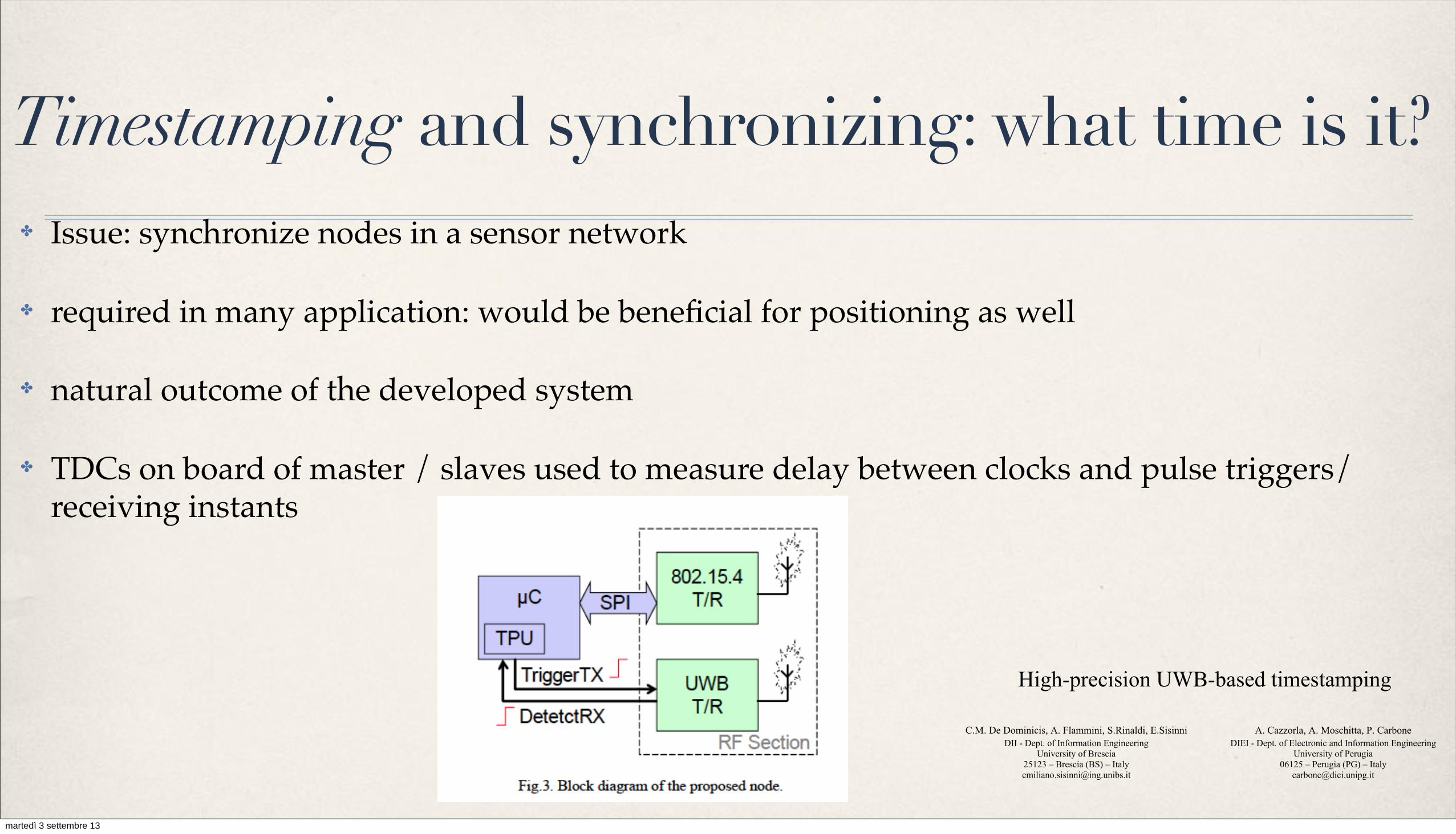
Timestamping and synchronizing: what time is it?✤ Issue: synchronize nodes in a sensor network
✤ required in many application: would be beneficial for positioning as well
✤ natural outcome of the developed system
✤ TDCs on board of master / slaves used to measure delay between clocks and pulse triggers/receiving instants
High-precision UWB-based timestamping
C.M. De Dominicis, A. Flammini, S.Rinaldi, E.Sisinni DII - Dept. of Information Engineering
University of Brescia 25123 – Brescia (BS) – Italy [email protected]
A. Cazzorla, A. Moschitta, P. Carbone DIEI - Dept. of Electronic and Information Engineering
University of Perugia 06125 – Perugia (PG) – Italy
Abstract— The work presented in this paper is related with time synchronization for wireless networks. In particular, it is focused on the proposal and experimental evaluation of a low-cost and high precision timestamping technique based on Ultra Wide Band (UWB) signalling. In recent years, the use of such systems has gained an increasing success thanks to their robustness to interferers and multipath. In this paper a new hybrid wireless node is proposed; a traditional IEEE802.15.4 radio, the reference physical layer for wireless sensor networks, is supported by an UWB transceiver. The former is used for communication purposes and allows to preserve compatibility with already installed infrastructures/networks; the latter is used for time of arrival estimation. Hardware prototypes have been realized and experimental tests have shown a sub-nanosecond accuracy. A comparison with commercial solutions has shown a performance improvement with respect to conventional approaches.
Keywords - synchronization; wireless sensor network; distributed systems; UWB systems
I. INTRODUCTION In recent years we have witnessed the proliferation of
wireless systems, mainly justified by the flexibility offered by cable removal. It is obvious that both the deployment and maintenance costs can be lowered using a completely autonomous device. In particular, recent advances in radio and embedded systems have enabled the proliferation of wireless sensor networks (WSNs), that are used in very different environments to perform various monitoring tasks. It must be said this success is also motivated by the availability of several reference standards, which allow interoperability among products of different vendors. For instance, low cost and robust radios compliant with the physical layer of the IEEE802.15.4 standard, have been used as the basis for many commercial and industrial solutions, such as the well known ZigBee, WirelessHART and ISA100.11a.
Regardless of the application field, the integration of all the readouts coming from a smart environment is possible if and only if also temporal information is available, i.e. when measurement of the variables of interest occurs. As a consequence all nodes within a WSN must share a common sense of time. In some situations a simple temporal ordinal scale (i.e. one event is occurred before/after another one) is
sufficient, but in most cases, a precise time reference is needed (i.e. the nodes must be clock synchronized). Referring to cabled communication systems, many approaches have been tried, from token passing, to conventional clock synchronization protocols, such as the IEEE1588 [1]. In particular, the basic idea behind this latter approach is to exploit message exchange not only to carry measurements but also time data. In particular, two nodes can be synchronized by exchanging packets of time of arrival (TOA) information, observed with their local clocks.
Taking the same approach also for wireless communications is a more difficult task, since the radio signal propagation is strongly affected by the environment [2]. Consider for example the biasing effect of multipath and non-line-of-sight (NLOS) situations. For all of these reasons the detection of the first arrived signal is a tricky task, especially considering that commercial transceivers usually optimize the probability of correct symbol detection and discard information about low power signals, as the line-of-sight (LOS) signals often are. Similar requirements often arise when using localization algorithms. In fact, trilateration needs knowledge of the distances among nodes, and these distances are usually estimated using the TOA of a radio signal (pseudorange) [3]. Many studies address this topic, identifying the most significant parameters and performance metrics. For instance, the positioning accuracy is known to improve with signal bandwidth. This suggests two possible strategies for nodes synchronization, the first one based on conventional modulation schemes coupled with some form of “pulse compression”, the second one based on Ultra Wideband (UWB) pulses. The former is simpler and less accurate, and viceversa.
The aim of this paper is to suggest a hybrid approach that mixes advantages of both strategies: the use of a standard radio preserves compatibility with pre-existing infrastructure/networks, while UWB pulses guarantee fine grain synchronization.
II. SYNCHRONIZATION OF A WSN The peculiar characteristics of a WSN strongly affect
also requirements of time synchronization protocols: scalability, low cost and low power consumption are compulsory issues. A rough classification of synchronization
978-1-61284-893-8/11/$26.00 ©2011 IEEE
martedì 3 settembre 13

Timestamping & Synchronizing✤ Transfer timing information
between transceivers for synchronization purposes
✤ Standard deviation:
✤ - using counter: < 1 ps
✤ - using TDC: < 19 psRubidium Atomic Clock HP 3225 B
Agilent 53131A
UWB Master
UWB Slave
DetectRx
3 m
TriggerTx
To this aim, the TriggerTX digital line of an UWB master node has been driven by a 1 MHz square wave, provided by HP 3225B function generator. The HP 3225B has been disciplined using a very stable frequency reference, provided a Stanford Research PRS10 rubidium atomic clock, with a 10 MHz output signal and a short term stability of 5·10-12. The output of the function generator has been initially acquired by an Agilent 53131A counter, obtaining a one-shot period measurement of 0.999 Ps, and a standard deviation of 1.56·10-15 s, evaluated over 100 consecutive one-shot measurements.
Subsequently, the counter has been replaced by the commercial TDC. In particular, 10 averaged “runs” have been carried out, each of them obtained by averaging 100 consecutive one-shot measurements. The ten values, plotted in Fig.7, have an overall average 1.000 Ps, and an overall standard deviation of 18.9 ps.
�
999.4
1 2 3 4 5 6 7 8 9 10run #
ns
999.2
999.6
999.8
1000.21000.4
1000.0
Fig. 7. Behavior of the commercial TDC over ten measurements obtained averaging 100 one-shot readouts.
Following the described activity, another experimental setup has been developed, aimed at measuring the jitter associated to the detection of an UWB pulse. The UWB transmitter is triggered as in the previous experiment. The setup is sketched in Fig.8.
Fig.8. Experimental setup to evaluate the timestamping capability.
This time, the pulser and the detector have been placed at a distance of 3m, i.e. well below the maximum allowable distance, in order to ensure a good SNR, and the repetition rate of the UWB pulses has been set to 500 kHz. As previously stated, the aim of these tests is to verify the feasibility of the proposed architecture. In particular, no particular attention has been devoted to the antenna design. A wide variety of UWB antennas are available in literature for different applications. For instance, if applicable,
directional antenna could be profitably used to reduce multipath effects in indoor environments. An automated measurement system has been realized to measure the period of the DetectRX digital line at the receiver side; to this aim, using the HP 53131A counter. In this way the UWB link quality has been verified.
First of all, the time distance between N=1000 consecutive couples of pulses has been collected; the frequency distribution of measurements around the source repetition rate is shown in Fig.9. The average value is ȝ=2.0002 ȝs and the standard deviation is ı=606.46 ps; the jitter, defined as the difference between maximum and the minimum period values is J=9.745ns, due to the presence of very few outliers.
-2 0 2 4 6 8 100
20
40
60
80
[ns]
Freq
uenc
y di
strib
utio
n [%
]
Fig.9. Frequency distribution around the source repetition rate of N=1000 couple of UWB pulses.
Supposing to send a train of equally separated impulses before the IEEE802.15.4 frame, performance can be improved by means of filtering. In order to verify this statement, 5 different runs of N=100 single period measurements have been collected, using again the setup of Fig. 6. The measurements frequency distribution of a single repetition around the source repetition rate is shown in Fig. 10. The average value is ȝ = 2.0002 ȝs and the standard deviation is ı = 522.96 ps; the standard deviation evaluated on the five average measurement results is ıAVG=107.66 ps; the jitter, defined as the difference between maximum and the minimum period values over the 5 runs, is JAVG=214.63 ps.
-0.5 0 0.5 1 1.5 2 2.50
10
20
30
40
50
[ns]
Freq
uenc
y di
strib
utio
n [%
]
Fig. 10. Frequency distribution around the source repetition rate of N=100
couple of UWB pulses
martedì 3 settembre 13

Serendipity or the law of unintended consequences
martedì 3 settembre 13

A low-cost (<50 euro) fast humidity sensor
✤ Measurement of humidity in woodchips of great interest in a growing market of wood stoves✤ Cable radar: pulse sent in closed-loop or open-ended wire, measured RTT✤ Time of flight as a function of medium effective dielectric constants✤ In turn, effective dielectric constant dependent on humidity surrounding cable: humidity sensor✤ all developed electronics ‘recyclable’ to realize sensor for humidity in wood-chips (or other material)
martedì 3 settembre 13

Systems
✤ Thermogravimetric Analysis (TGA) used as a reference (procedure described EN 14774-2 standard)
vs
martedì 3 settembre 13

Experimental results
5 10 15 20 25 30 35 4019
19.1
19.2
19.3
19.4
19.5
19.6
19.7
Humidity [%]
prop
agat
ion
time
[ns]
small sized woodchipmedium sized woodchiplarge sized woodchip
martedì 3 settembre 13

some unanticipated consequences ...
✤ Done most of my research career in signal processing (with some VLSI at an early stage)
✤ Is easy to understand and to touch research easier to be funded and more attractive?
✤ Provocativeness: interesting /curious application oriented problems attract more easily attention: more students to contribute, more colleagues willing to collaborate, easier to be communicated to the general public, easier to be financed: choice of research subject has consequences -> the value of research: method-led research vs problem-led research
✤ national/continental policies about research, drive choices for financing research projects: better apply some anticipative/adaptive (?) behavior
martedì 3 settembre 13

Conclusions
✤ A fascinating old problem: not a single solution, many competing technologies
✤ A system engineering type of problem: realizing an indoor positioning system from scratch using off-the-shelf components
✤ Although technical solutions are known, several technical issues must be solved, especially at the interface between sub-systems
✤ Signal processing must know properties of hardware solutions to optimize accuracy of estimates
✤ In the end, the outcome is a measurement instruments, whose performance in terms of position accuracy strongly depends on the adopted system integration approach
martedì 3 settembre 13