Outline Coordinate system for beam motion - IU Bphysics.indiana.edu/~shylee/p571/AAP_part_1.pdfHamiltonian 1/19/2015 5 After a series of canonical transformations, new Hamiltonian

1/19/2015 1

Lecture 1: Modeling Accelerators – Tracking particles in a transport line or a storage ring

X. HuangUSPAS, January 2015

Hampton, Virginia

X. Huang, USPAS Jan 2015

Goals and scope• Goals:

– Gain deeper understanding of single particle dynamics in storage rings.

– Understand how accelerator modeling codes work.– Learn to develop tracking codes to solve realistic problems.

• Scope:– Assumptions

• Motion of relativistic particles• Reference beam energy is fixed (no acceleration)• Large rings

– Collective effects are not covered.

1/19/2015 2X. Huang, USPAS Jan 2015

Outline• Coordinate system and Hamiltonian• Magnetic fields in accelerator elements• Beam motion in accelerator elements

– Linear model– Symplectic integration– Fringe field effects– Misalignments


Coordinate system for beam motion

1/19/2015 4

Reference orbit

Natural coordinate system The HamiltonianΦwith canonical momentum and the mechanical momentum

the vector potential.


Lecture Note Part 1 001

Hamiltonian

1/19/2015 5

After a series of canonical transformations, new Hamiltonian becomes1 1 with canonical coordinates , , , , , and free variable , and∙ 1 , ∙∙ ̂∙ 1 , ∙∙ ̂∙ , ∙ , 1 ∙ ̂,

, -1is the momentum of the reference particle.

Expanding (small angle approximation, valid for large rings)1 1 12 1 11Knowing the magnetic fields as given by the vector potential, we may solve for the motion of charged particles.


Vector potential for straight elements

1/19/2015 6

For magnets with straight geometry (curvature of orbit 0 , the vector potential is ! 0where / is magnetic rigidity (here as normalization constant), and are skew and normal multipole components, respectively. On the middle plane ( 0): , 0

, 0For quadrupole 2, 12sextupole 3, 16 3


Vector potential on curved orbit

1/19/2015 7

For elements with mid-plane symmetry, on the middle plane, the magnetic field is, 0, , 0, 0, 0, 2! ⋯The field may be represented with the vector potential ∙ ̂ ⋯ 3 ⋯ ⋯,, , , , 0.

So the Hamiltonian for a combined-function gradient dipole magnet ( 0) is:1 1 12 12with (usually ), . Linearize the Hamiltonian

2 1 2 2Here we dropped the term 1 , amounting to redefine coordinate to Δ .


Solving beam motion with Hamiltonian• Approach 1: particle tracking – numerically calculate the

canonical coordinates of particles through every accelerator element, for many turns if necessary. – To the linear order, tracking can be done with transfer matrix.– For nonlinear elements, symplectic integration is needed.

• Approach 2: transfer maps – building Lie maps or Taylor maps for individual accelerator elements and sections of accelerator (or a full ring). – Lie map for individual element is derived from the Hamiltonian.– Lie map for accelerator section can be obtained with Lie operator

concatenation.– Taylor maps can be obtained from the Lie maps or numerically with

TPSA.

1/19/2015 8

We will discuss the particle tracking approach.



Tracking through drift space

1/19/2015 9

The Hamiltonian for a drift space 2 1The equations of motion

, 0, 0

, 0The coordinates at the entrance (subscript 0) and exit (subscript 1) faces of a drift space with length is related by

,,

,,

,.

1


Tracking through quadrupole magnets

1/19/2015 10

For a quadrupole magnet (length , gradient the Hamiltonian is2 1 2Since momentum does not change in this magnet, we first change the canonical momentum coordinates to p ′, p ′, by scaling down the Hamiltonian to 1 12 2 1Particle coordinates , , , , , ) at entrance and exit faces are connected by , with transfer matrix given by0 00 00 0With , and10 1


Tracking through quadrupole – cont’d

1/19/2015 11

0 cosh sinhsinh cosh

0 cos sinsin cos

After applying the transfer matrix, the original canonical momentum coordinates can be restored.

Element can be derived from equation2and for 0, 1 cos sin , 1 cosh sinh ,


Tracking through dipole magnets – linear

1/19/2015 12

Keeping linear optics terms, the Hamiltonian is .Again change the momentum coordinates, the new Hamiltonian is12 2 1 2 1 1Similarly the transfer matrix for , , , , , ) is00 00With / , and 00 , 0 0With (for / 0) 1 cosh / sinh /



Tracking through dipoles – linear (cont’d)

1/19/2015 13

For / 01 cos / ,.

Element can be derived with12 1and , as given properly with the transfer matrix (with ).The canonical momentum coordinates are restored after applying the transfer matrix.

The above tracking solutions for quadrupole and dipole elements treat momentum deviation properly such that linear optics of off-momentum particles is accurate.


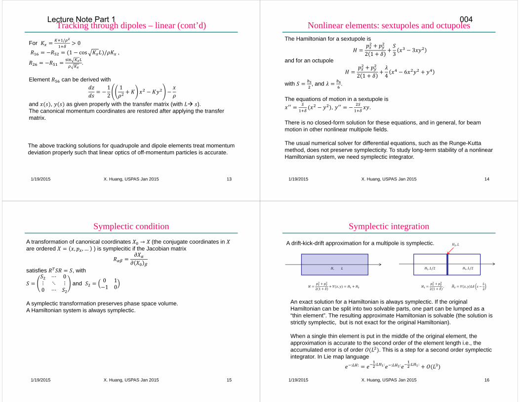
Nonlinear elements: sextupoles and octupoles

1/19/2015 14

The Hamiltonian for a sextupole is2 1 3 3and for an octupole 2 1 4 6with , and .

The equations of motion in a sextupole is, .

There is no closed-form solution for these equations, and in general, for beam motion in other nonlinear multipole fields.

The usual numerical solver for differential equations, such as the Runge-Kuttamethod, does not preserve symplecticity. To study long-term stability of a nonlinear Hamiltonian system, we need symplectic integrator.


Symplectic condition

1/19/2015 15

A transformation of canonical coordinates → (the conjugate coordinates in are ordered , , … ) is symplecitic if the Jacobian matrix

satisfies , with ⋯ 0⋮ ⋱ ⋮0 ⋯ and 0 11 0A symplectic transformation preserves phase space volume. A Hamiltonian system is always symplectic.


Symplectic integration

1/19/2015 16

A drift-kick-drift approximation for a multipole is symplectic.

2 1 , 2 1 , , 2, /2 , /2

,,

An exact solution for a Hamiltonian is always symplectic. If the original Hamiltonian can be split into two solvable parts, one part can be lumped as a “thin element”. The resulting approximate Hamiltonian is solvable (the solution is strictly symplectic, but is not exact for the original Hamiltonian).

When a single thin element is put in the middle of the original element, the approximation is accurate to the second order of the element length i.e., the accumulated error is of order . This is a step for a second order symplecticintegrator. In Lie map language: : : : : : : :



Fourth order symplectic integrator

1/19/2015 17

Higher order (more accurate) symplectic integrators can be constructed based on the lower order ones. The next order symmetric integrator is fourth order.

,

,

,,,

, ,

The coefficients are0.6756035959798286638, with 1 20.1756035959798286639,2 1.351207191959657328,2 1.702414383919314656.Note and are negative!

Symplectic integration for straight geometry multipoles is simple, just splitting the Hamiltonian into drifts and multipole kicks.


Symplectic integration for dipoles

1/19/2015 18

How to split the Hamiltonian of a dipole?1 1 12 ,(1) The drift-kick split, 1 1 , drift in curvilinear reference system., , bend and multipole kick

Solution to : , with tan .

1 sin ,cos tan sin ,1 cos tan sin ,

, .


Cont’d

1/19/2015 19

Drift in a curvilinear system.

(2) The bend-kick split (E. Forest)1 1 , a pure sector dipole, , multipole kick

An issue with this approach: the origin of local reference system at does not transfer to the origin at .

The solution may be to subtract this offset error.

X. Huang, USPAS Jan 2015 1/19/2015 20

Solution to the sector dipole Hamiltonian:1 ,cos 1 sin ,sin sin ,sin sin ,

, .

(3) Simplified approach: straight drift + bend/multipole kick2 1 2 ,With

, drift on straight reference system., , bend and multipole kick



Accuracy of symplectic integrator

1/19/2015 21

0 2 4 6 8 10 1210-8

10-6

10-4

10-2

100

x0 (mm)

x

(mra

d)

Quad: L=0.5 m, K=1.2 m-2

Nslice=1Nslice=4Nslice=10

Symplectic integrator may give different results than the linear transfer method because of integration errors. Slicing the thick element into more equal pieces (in other words, reducing integration step size) help improve accuracy.

Example: errors to kick Δ ′ for a quadrupole for the fourth order integrator.


RF cavity

1/19/2015 22

RF cavity is usually modeled as a thin element. The voltage on the RF gap may be given by sinThe reference particle arrives at 0. The frequency must be a multiple of the revolution frequency 2 2Since , the change to momentum deviation is sin

Transfer matrix for an RF cavity for ( , coordinates1 01 1 0cos 1


Orbit correctors

1/19/2015 23

Orbit correctors can be modeled as thin elements (may be sandwiched with drift spaces). Unlike bending magnets, the reference orbit is not changed by the correctors.

The kick angles , are specified for the reference particle.

(noting that , and 1 and similarly for the -plane.

Orbit correctors cause changes to the closed orbit.


Misalignment• Complete description of the misalignment of an element include 6

parameters

• Misalignment can be modeled as coordinate transformations at the entrance and exit faces of the element.

• Simplified form of these transformations can be used.– At entrance, Δ , Δ , 1 , 1

plus rotation about axis with angle .– At exit, rotation about axis with angle , followed by Δ , Δ , 1 , 1 .

1/19/2015 X. Huang, USPAS Jan 2015 24

Δ , Δ , Δ displacements along axis of local coordinate system.( , , rotation about the , and axis, respectively.

Δ Δ


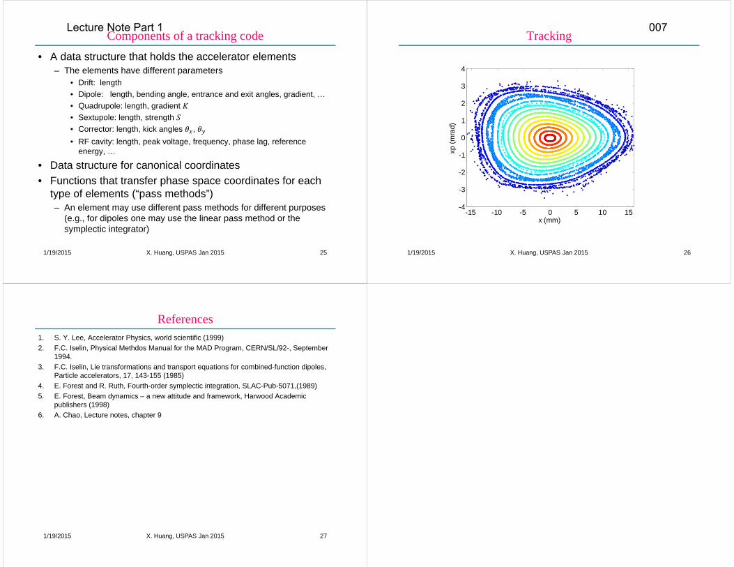
Components of a tracking code• A data structure that holds the accelerator elements

– The elements have different parameters• Drift: length• Dipole: length, bending angle, entrance and exit angles, gradient, …• Quadrupole: length, gradient • Sextupole: length, strength • Corrector: length, kick angles , • RF cavity: length, peak voltage, frequency, phase lag, reference

energy, …

• Data structure for canonical coordinates• Functions that transfer phase space coordinates for each

type of elements (“pass methods”)– An element may use different pass methods for different purposes

(e.g., for dipoles one may use the linear pass method or the symplectic integrator)

1/19/2015 25X. Huang, USPAS Jan 2015

Tracking

1/19/2015 26

-15 -10 -5 0 5 10 15-4

-3

-2

-1

0

1

2

3

4

x (mm)

xp (m

rad)


References1. S. Y. Lee, Accelerator Physics, world scientific (1999) 2. F.C. Iselin, Physical Methdos Manual for the MAD Program, CERN/SL/92-, September

1994.3. F.C. Iselin, Lie transformations and transport equations for combined-function dipoles,

Particle accelerators, 17, 143-155 (1985)4. E. Forest and R. Ruth, Fourth-order symplectic integration, SLAC-Pub-5071,(1989)5. E. Forest, Beam dynamics – a new attitude and framework, Harwood Academic

publishers (1998)6. A. Chao, Lecture notes, chapter 9

1/19/2015 27X. Huang, USPAS Jan 2015


1/19/2015 1

Lecture 2: Modeling Accelerators – Calculation of lattice functions and parameters


Hampton, Virginia


Outline• Closed orbit• Transfer matrix, tunes, Optics functions• Chromatic effects: dispersion function, chromaticity• Radiation integrals and lattice parameters• Characterization of nonlinear dynamics• Dynamic aperture and momentum aperture from tracking


Calculation of closed orbit• Closed orbit is the fixed point of the one-turn map (

1/19/2015 3

If the one-turn map is linear, i.e. 0 Δwhere 0 is the transfer matrix on the reference orbit and Δ is the accumulated coordinate displacement after one turn, then the closed orbit is0 ΔFor the general nonlinear case, can be found numerically with iteration.

Here the map is evaluated with tracking.

Closed orbit differs from the design orbit when the guiding magnetic fields deviate from the ideal values (field errors or misalignment) or there is an energy error.


• Closed orbit with fixed momentum deviation (useful for computing optics functions).

• Closed orbit with fixed frequency – situation in real machine. – Closed orbit in full 6D phase space.– The above iterative procedure is valid, using 6 6 matrix and full vector. – RF cavity, radiation damping can be turned on.

1/19/2015 4

Starting with 0,0,0,0,0, , at iteration

Also calculate , the 4 4transverse transfer matrix about . Then the next iteration moves to

where superscript " 4 " indicates vector with the first 4 coordinates, the longitudinal coordinates are fixed at 0, .



Transfer matrix• Each element may generate its own transfer matrix internally. The

transfer matrix for a section or a full ring is the product of the transfer matrices of the elements.

• The transfer matrix for an element, a section or a full ring can also be obtained from tracking with numerical differential.

1/19/2015 5

0 1 2 …→ → → … →

To find the transfer matrix around orbit , , , , , (e.g., the reference orbit 0,0,0,0,0,0 , tracking particlesΔ Δ , Here represents the map from location 0 to 1,Δ Δ , which is evaluated with tracking.Δ , 0, 0, 0, 0, 0 , with small quantity ~10 ~10 .Then the column corresponding to coordinate 1 ( is

: , Δ Δ2Similarly for the other columns.


TRANSPORT map• TRANSPORT map is an extension of transfer matrix to second order

(Taylor map).

• For an element with a constant Hamiltonian (no -dependence), the second order TRANSPORT map can be derived from second and third order polynomials in the Hamiltonian.

• TRANSPORT map is generally not symplectic. But it can be useful for one-pass system.

• Combination of TRANSPORT maps ( → , → ).

1/19/2015 6

, , , 1…6,Summation of identical indices is assumed. Note by convention (making symmetric), .

0 1 2, ,

, .


Calculating TRANSPORT map with numerical differential

1/19/2015 7

For , tracking particles (from location 0 to 1)0 ,Δ Δ , Δ Δ ,Example: Δ , 0, 0, 0, 0, 0 , with small quantity ~10 ~10 .Then the elements corresponding to coordinate 1 ( , , ( 1. . 6 is

:, Δ Δ 2 02For , tracking particles (assuming 1, 2), Δ , , Δ , , , , 0, 0, 0, 0, Δ , , Δ , , , , 0, 0, 0, 0, Δ , , Δ , , , , 0, 0, 0, 0, Δ , , Δ , , , , 0, 0, 0, 0Then : : 18 , , , ,


Linear optics for a storage ring (uncoupled)• Assuming there is no coupling, the one-turn transfer matrix looks

like

• Courant-Snyder parameterization of the one turn matrix

1/19/2015 8

00 00where , and are 2 2 matrices. The horizontal and vertical optics functions can be determined from and , respectively.

cosΦ sinΦ sinΦ1 sinΦ cosΦ sinΦWith Φ 2 , and the tune.

Caution: When using tracking to compute linear optics, elements with time dependence or elements that change momentum deviation (like RF cavity) should be turned off.



Tune and Twiss functions• The tune can be determined from

• Twiss functions at the location of the one-turn matrix

• Propagation of Twiss functions to another location (knowing transfer matrix → )

• Phase advance

1/19/2015 9

cosΦ , sinΦ signtan . ,

,

.

0 1→

ΔΦ Φ Φ tanX. Huang, USPAS Jan 2015

Linear optics (coupled)• With coupling, the 4 4 matrix of the transverse phase space is

• Decoupling: with a coordinate transformation , such that the transfer matrix for is block diagonal (decoupled), i.e., for , with

1/19/2015 10

where , , , are all 2 2 matrices. The , motion are coupled when , 0 . In this case, the tunes derived from and are inaccurate.

00 , and The transformation matrix can be computed.

where is the symplectic conjugate of (required such that is symplectic)


• Remarkably, elements of the matrix can be directly computed from the original matrix.

• Tunes and Twiss functions can be computed from decoupled transfer matrices and (blocks in the matrix) in the same manner as the uncoupled case.

1/19/2015 11

Symplecticity of also leads to 1The reverse matrix is

TrTr | |, and TrTr | |,where .


Dispersion function and chromaticity• By definition dispersion is the differential closed-orbit w.r.t. momentum

deviation.

• Numerical calculation by off-momentum closed orbit (fixed momentum).

• Chromaticities are calculated with numerical differential of the tunes w.r.t. momentum deviation.

1/19/2015 12

The first order and second order dispersion functions are defined through0 12where , , , and similarly for .



Dispersion function from transfer matrix• The one-turn transfer matrix is

• Propagation of dispersion

1/19/2015 13

With 0000The closed orbit with an infinitesimal momentum deviation would be , 0,1 . From

One gets :where : , , , . Therefore :

→ : →X. Huang, USPAS Jan 2015

Momentum compaction factor• Momentum compaction factor (MCF) is defined

• MCF is related to one-turn transfer matrix element

• Calculating MCF with tracking.

1/19/2015 14

1 Δ 1Higher order momentum compaction factorsΔ 12 ⋯

sin 2where / is the local dispersion invariant. Usually / is a good approximation.

1. Calculate the closed orbit for and (using ~10 10 )with fixed momentum deviation, to get and .2. Set the coordinate in to 0. Then track the closed orbits for one turn

), ),3. The MCF is 2

2nd order MCF can be computed similarly.


Radiation integrals. • Radiation integrals are related to important lattice parameters for

electron storage rings. • Definition

• For , and , integration needs to consider variation of dispersion and Twiss functions (for ) inside the magnets. This can be done analytically, with

1/19/2015 15

∮ , ∮ , ∮ | | ,∮ 2 , with ∮ .

cos sin , for 0cosh sinh , for 0,

and formulas for and .


Lattice parameters

• Lattice parameters

1/19/2015 16

Note: and change at the dipole edges due to edge focusing! tan , tanwhere is the entrance angle and subscript ‘ ’ indicate values before the edge ( and are continuous at the edge).

Parameters Formulas

Energy loss per turn keV 14.085 GeVMomentum spread 2Horizontal emittance

Damping partition 1 , 1, 2Damping time , , 2, ,



Precise tune determination from tracking data• To characterize nonlinear dynamics of a storage ring, it is often useful

to determine tunes from tracking or measured turn-by-turn data for beam with various energy error or oscillation amplitude.

• Simple FFT is not accurate (precision ~1/ )• NAFF (numerical analysis of fundamental frequency) is a method to

accurately determine the tune from turn-by-turn data.

1/19/2015 17

Assume a discrete sampling of a quasi-periodic signal s cos 2( may have small secular drifting) iscos 2 , 1, 2, … ,with sampling frequency 1/ and / . How to determine from the data?

NAFF: find the frequency ̅ ̅ that maximizes the overlap between the power contents of and exp 2 ̅ , i.e.̅Then ̅ is a precise approximation to .


NAFF – cont’d

• Numerical experiment

1/19/2015 18

The function (window function) is a data filter, added to improve accuracy. A good choice is the . .

Data cos 2 , 1… , random drawn Gaussian distribution with 0, )

Error No noise .N=32 -5.7e-06 -1.3e-04N=64 -5.9e-08 7.3e-05N=128 2.5e-09 -1.3e-07N=256 1.1e-10 -4.9e-06


Characterization of nonlinear dynamics• The motion of particles with large oscillation amplitude

(nonlinear dynamics) is critical to storage ring performance.• Common indicators of beam nonlinear dynamics

– Nonlinear chromaticity (tune shifts with momentum deviation)– Tune shifts with amplitude– Tune diffusion– Frequency map– Resonance driving terms

• Direct measures of nonlinear dynamics performance– Dynamic aperture– Momentum aperture

1/19/2015 19X. Huang, USPAS Jan 2015

Nonlinear chromaticity• First order chromaticities are usually corrected to a small positive

number (with sextupoles). The higher order chromaticities may dominate the ~ behavior.

• Tracking setup: correct linear chromaticity to zero, turn off cavity (fixed momentum deviation), small initial , offsets, track 256 to 1024 turns.

• Example: SPEAR3

1/19/2015 20

-0.04 -0.03 -0.02 -0.01 0 0.01 0.02 0.03 0.040.1

0.12

0.14

0.16

0.18

0.2

0.22

0.24

x,y

x

y

0.05 0.1 0.15 0.20.1

0.15

0.2

0.25

0.3

1,-1,0 1,-2,02,-1,0 2,-2,0

3,-1,0

0,4,1

1,3,1 2,2,1

1,-4,-1

2,-3,03,-2,0

4,-1,0 0,5,1

1,4,1

2,3,1 3,2,1 4,1,15,0,1

1,-5,-1

2,-4,-1

2,-4,03,-3,04,-2,0

5,-1,0

0,6,1

1,5,1

2,4,1

3,3,1

4,2,1 5,1,16,0,1

x

y



Amplitude-dependent tune shifts• Nonlinear elements cause dependence of betatron tunes

over oscillation amplitude.

• Numerical calculation of amplitude-dependent tune shifts.

1/19/2015 21

, 2 2 2 2, 2 2 2 2where / , and likewise for .

In general, .

The coefficients can be computed with formulas.

Track particles with small initial offset and a series of offsets, obtain tunes for each initial offset, fit and vs. with linear model. Repeat for dependence.


Cont’d

1/19/2015 22

0 0.5 1 1.5 2 2.5 3

x 10-5

0.105

0.11

0.115

0.12

x

0 0.5 1 1.5 2 2.5 3

x 10-5

0.175

0.18

0.185

0.19

x2 (m2)

y

0 0.5 1 1.5 2 2.5 3 3.5 4 4.5

x 10-6

0.1055

0.106

0.1065

0.107

0.1075

x

0 0.5 1 1.5 2 2.5 3 3.5 4 4.5

x 10-6

0.177

0.1772

0.1774

0.1776

0.1778

y2 (m2)

y

An example: SPEAR3The coefficients are2 2

2 2 1900 21302110 1760X. Huang, USPAS Jan 2015

Frequency map• A more complete revelation nonlinear behavior is the

frequency map analysis (FMA).

1/19/2015 23

With initial transverse position coordinates and distributed on a grid (all other coordinates set to zero), find the corresponding betatron tunes and tune diffusion. , → ,

Steier, Robin, EPAC 2000

Frequency map for the ALS ideal lattice.


Evaluation of dynamic aperture• Dynamic aperture (DA) is the (single particle dynamics)

stability region around the reference orbit. Large DA is critical for storage ring performance (injection efficiency and lifetime).

• DA is evaluated in simulation with tracking.– Long term tracking is needed (one damping time or more for

electron storage rings).– 6D phase space tracking with radiation damping. – To be realistic, model may include insertion device effects,

systematic errors and random errors of magnets.– Multiple random error seeds are used. – Physical apertures may also be included in the model.– Tracking may start at the injection point (septum magnet).

1/19/2015 24X. Huang, USPAS Jan 2015


1/19/2015 25

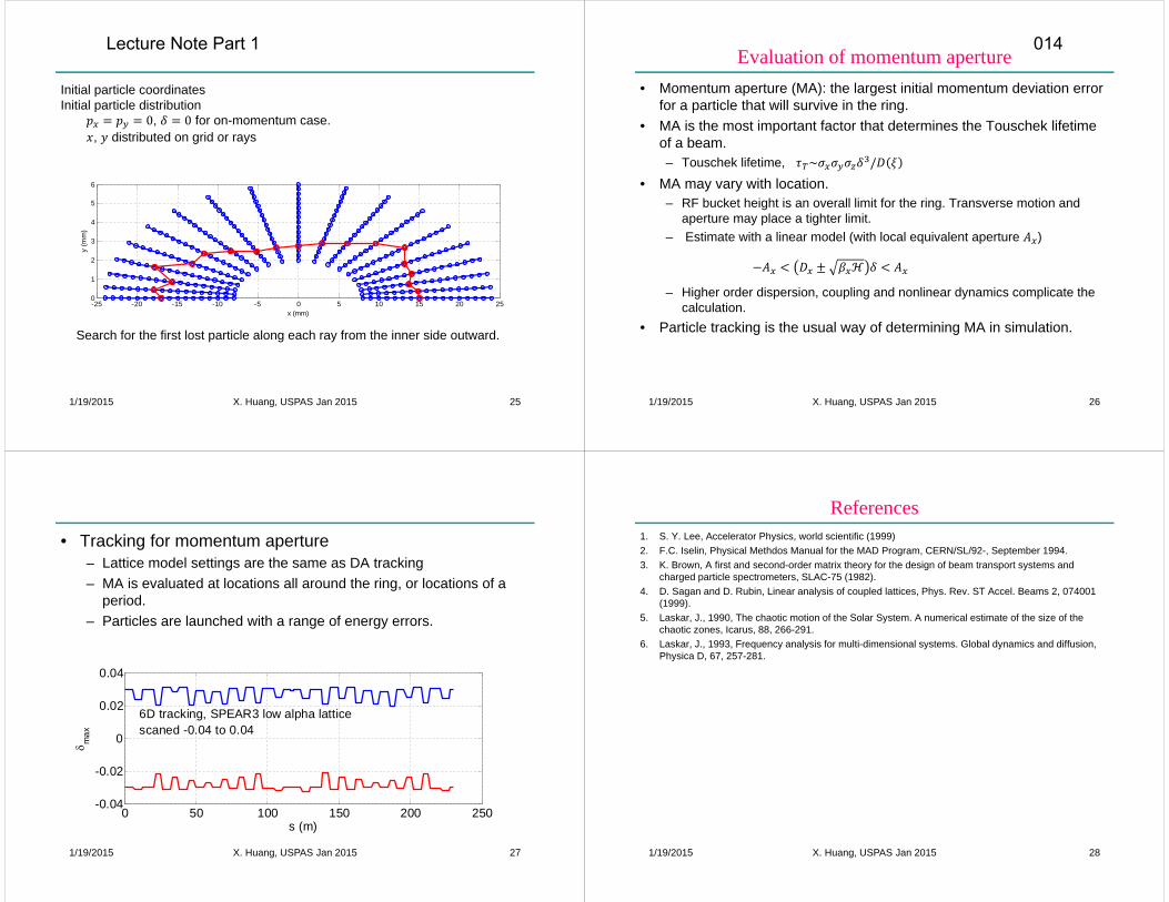
Initial particle coordinatesInitial particle distribution0, 0 for on-momentum case.

, distributed on grid or rays

-25 -20 -15 -10 -5 0 5 10 15 20 250

1

2

3

4

5

6

x (mm)

y (m

m)

Search for the first lost particle along each ray from the inner side outward.


Evaluation of momentum aperture• Momentum aperture (MA): the largest initial momentum deviation error

for a particle that will survive in the ring.• MA is the most important factor that determines the Touschek lifetime

of a beam. – Touschek lifetime, ~ /

• MA may vary with location.– RF bucket height is an overall limit for the ring. Transverse motion and

aperture may place a tighter limit.– Estimate with a linear model (with local equivalent aperture )

– Higher order dispersion, coupling and nonlinear dynamics complicate the calculation.

• Particle tracking is the usual way of determining MA in simulation.

1/19/2015 26X. Huang, USPAS Jan 2015

• Tracking for momentum aperture– Lattice model settings are the same as DA tracking– MA is evaluated at locations all around the ring, or locations of a

period. – Particles are launched with a range of energy errors.

1/19/2015 27

0 50 100 150 200 250-0.04

-0.02

0

0.02

0.04

s (m)

max

6D tracking, SPEAR3 low alpha latticescaned -0.04 to 0.04


References1. S. Y. Lee, Accelerator Physics, world scientific (1999) 2. F.C. Iselin, Physical Methdos Manual for the MAD Program, CERN/SL/92-, September 1994.3. K. Brown, A first and second-order matrix theory for the design of beam transport systems and

charged particle spectrometers, SLAC-75 (1982).4. D. Sagan and D. Rubin, Linear analysis of coupled lattices, Phys. Rev. ST Accel. Beams 2, 074001

(1999).5. Laskar, J., 1990, The chaotic motion of the Solar System. A numerical estimate of the size of the

chaotic zones, Icarus, 88, 266-291.6. Laskar, J., 1993, Frequency analysis for multi-dimensional systems. Global dynamics and diffusion,

Physica D, 67, 257-281.

1/19/2015 28X. Huang, USPAS Jan 2015


1/19/2015 1

Lecture 3: Modeling Accelerators – Fringe fields and Insertion devices


Hampton, Virginia


Outline• Fringe field effects

– Dipole– Quadrupole

• Modeling of insertion devices• Radiation damping and quantum excitation

– Damping, excitation, Ohmi envelope

• Longitudinal tracking with acceleration


Magnetic field profile and the hard-edge model• Most accelerator modeling codes use the hard-edge model for magnet

– constant Hamiltonian.• Real magnets always have a smooth transition at the edges – fringe

fields.

• Hard edge model– Field or gradient is a constant equal to the average value inside the magnet body.– The effective length is the integrated strength divided by the field or gradient.

1/19/2015 3

-1 -0.5 0 0.5 10

0.5

1

1.5

Z (m)

By/

Bym

ax

RADIA newMeasured 2001fit meas 2001measured 2007

-0.4 -0.3 -0.2 -0.1 0 0.1 0.2 0.3 0.4 0.5 0.60

2

4

6

8

10

12

14

16

18

Z (m)

B1 (T

/m)

all quads at 72 A in modeling

60Q50Q34Q15Q

SPEAR3 dipole ~ SPEAR3 quadrupoles ~

The hard-edge model is non-maxwellian!X. Huang, USPAS Jan 2015

Vector potential with fringe field• With cylindrical symmetry, the vector potential of a normal multipole

( 1 for dipole, etc.) with fringe field (with Coulomb gauge ∙ 0) on a straight geometry is

1/19/2015 4

! ∑ , ,

! ∑ , ,

! ∑ , .With cos and sin and, 1 ! ! ! , , and , , .

Example: for dipole 1, assuming , Θ , thenΘ 4 , Θ′ 4Θ B Θ 5 .Correspondingly, the magnetic field isΘ′′ , Θ Θ′′ 3Θ .



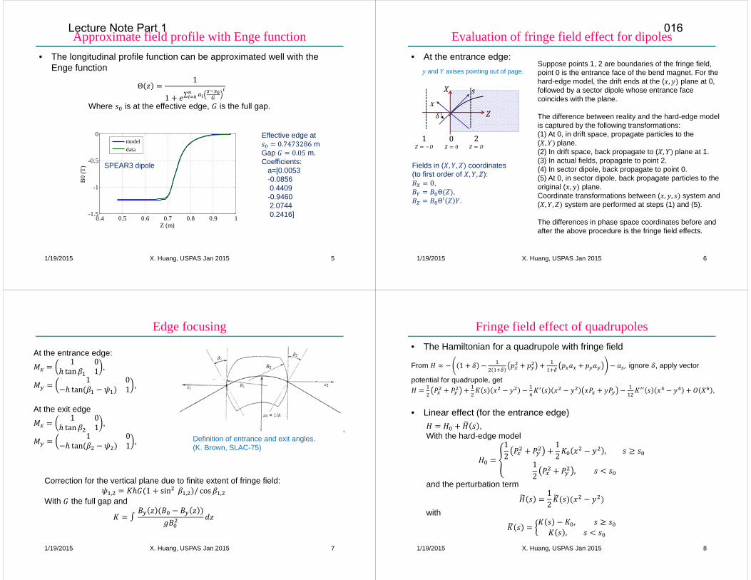
Approximate field profile with Enge function• The longitudinal profile function can be approximated well with the

Enge function

1/19/2015 5

Θ 11 ∑Where is at the effective edge, is the full gap.

0.4 0.5 0.6 0.7 0.8 0.9 1-1.5

-1

-0.5

0

Z (m)

B0 (T

)

modeldata

SPEAR3 dipole

Effective edge at 0.7473286 mGap 0.05 m.Coefficients:

a=[0.0053-0.08560.4409

-0.94602.07440.2416]


Evaluation of fringe field effect for dipoles• At the entrance edge:

1/19/2015 6

and axises pointing out of page.

0 01 2

Suppose points 1, 2 are boundaries of the fringe field, point 0 is the entrance face of the bend magnet. For the hard-edge model, the drift ends at the ( , plane at 0, followed by a sector dipole whose entrance face coincides with the plane.

The difference between reality and the hard-edge model is captured by the following transformations:(1) At 0, in drift space, propagate particles to the ( , plane.(2) In drift space, back propagate to ( , plane at 1.(3) In actual fields, propagate to point 2.(4) In sector dipole, back propagate to point 0.(5) At 0, in sector dipole, back propagate particles to the original ( , plane.Coordinate transformations between ( , , system and ( , , system are performed at steps (1) and (5).

The differences in phase space coordinates before and after the above procedure is the fringe field effects.

Fields in ( , , coordinates (to first order of , , ):0, Θ ,Θ .


Edge focusing

1/19/2015 7

At the entrance edge:1 0tan 1 ,1 0tan 1 ,

At the exit edge1 0tan 1 ,1 0tan 1 , Definition of entrance and exit angles.(K. Brown, SLAC-75)

Correction for the vertical plane due to finite extent of fringe field:, 1 sin , / cos ,With the full gap and


Fringe field effect of quadrupoles• The Hamiltonian for a quadrupole with fringe field

• Linear effect (for the entrance edge)

1/19/2015 8

From 1 ,ignore , apply vector

potential for quadrupole, get,

,With the hard-edge model12 12 ,12 , and the perturbation term 12with , ,



• Linear effect as a thin element

1/19/2015 9

Transfer matrix1 → 2 1 → 0 0 → 2The generating function for map* : : is calculated to be 2With integral defined as

The transfer matrix is diag , , , .

0 01 2

At the exit edge, integral has opposite sign. So the two edges tend to cancel. The cancellation is not complete for quadrupoles with finite length. The net effect includes a tune shift (always negative)

||2

|,|2 0

120

0

120

KILK

KILK y

yx

x

With 2 being the fringe length, roughly

*The Lie map : : 1 : : ! : : ⋯ is an operator, where ∶ : , , Poisson bracket. The Lie map for a constant Hamiltonian is : :.


Nonlinear effect of quadrupole fringe field• Apply the same approach to find the generating function for nonlinear

effects (the map is : :). For the entrance edge (change sign for the exit edge).

1/19/2015 10

112 3 3This cannot be symplectically integrated. However, the generating function for a skew quadrupole is integrable. , 6exp : : , exp : : 3 ,Similarly for the term. These are two kicks!

Therefore, we can model the nonlinear effects of quadrupole fringe field with a symplectic map by rotating , applying the skew quad fringe kick , and rotating back.


Example

1/19/2015 11

xyzBzB

xyxzzxBB

yyxzzyBB

z

y

x

)(')sgn(

)]3)((''121)([

)]3)((''121)([

1

231

321

Magnetic field

0 0.1 0.2 0.3 0.4 0.5 0.6 0.70

0.5

1

1.5

Z (m) for 60Q

B1f

(nor

mal

ized

)

m 060.06 ,m 1061.00

123

0

11

kI

kII a

SPEAR3 quadrupole fringe field

0.02 0.02 0.02 0.02 0.02 0.02 0.02

-0.0123

-0.0123

-0.0123

-0.0123

-0.0123

-0.0122

-0.0122

-0.0122

xi (m)

xpf (r

ad)

quadpassquadpass+matrixnew quad passfield pass

Case ElementQuadLinearPass QuadQuadLinearFPass QuadField Pass + Quad Field

[Drift QuadFieldDrift]


Insertion device modeling• Wiggler and undulator

1/19/2015 12

On the mid-plane, the magnetic fieldcosTrajectory coswith amplitude .

,

Wiggler parameter 0.934 T cm .

with .



Magnetic field in an ID• The field is periodic in the longitudinal direction.

1/19/2015 13

Suppose the vertical field is , coswith symmetry , , and , , . It can be shown that to satisfy ∙ =0 and =0, we need0The other field components, cos ,, cos .Symmetry leads to 0 0, 0 0 and 0 0.

The Halbach wiggler field modelcosh cosh cos ,sinh sinh cos ,cosh sinh cos .

with .


Effects of ideal ID on the beam• The Hamiltonian for the Halbach model (to 4th order)

• Linear effect

• Nonlinear effects

– Octupole-like effect causing amplitude-dependent tune shift, ∝ 1/19/2015 14

32 .

Assume 0 (ideal planar wiggler with wide poles)12 4 sin2 12For the ideal planar wiggler, the effect on beam is on the vertical plane.

Tune shift: Δ ∗8 96 ∗where is wiggler length, ∗ is beta function at ID center (minimum)


Effects of an imperfect wiggler

1/19/2015 15

Kick to the beam (by field integral on trajectory)Δ 1 , ,1 , , 1 ΔStatic dynamic

Static field integrals (on straight path):First integral , 0, , Δ /Second integral , 0, ̅ ̅, Δ /(similarly for and )Quadrupole int. , Δ , ΔSkew quad int. , coupling

Sextupole int. , nonlinear dynamics…

The field integrals can be obtained from measurements. These static effects can be modeled as multipole kicks.


Dynamic effects from field roll-off

1/19/2015 16

Kick from the dynamic effectΔ Δ ,withΔ cos , , cos , (on the mid-plane)So the kick is Δ 12 , 0The dynamic kick effect is particularly severe for elliptically-polarized undulator(EPU)

Field roll-off of the planar phase for an EPU Dynamic integral from the field roll-off

I. Blomqvist



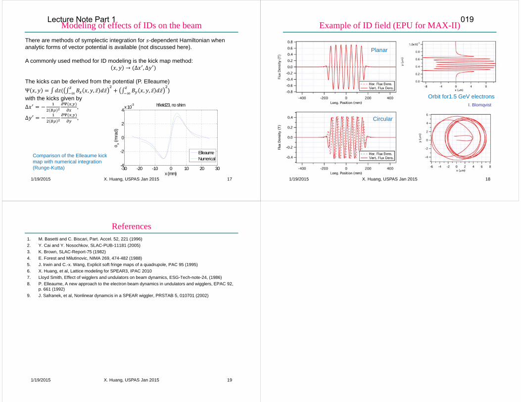
Modeling of effects of IDs on the beam

1/19/2015 17

There are methods of symplectic integration for -dependent Hamiltonian when analytic forms of vector potential is available (not discussed here).

A commonly used method for ID modeling is the kick map method:, → Δ , ΔThe kicks can be derived from the potential (P. Elleaume)Ψ , , , ̅ ̅ , , ̅ ̅ )with the kicks given byΔ , , Δ , ,

-30 -20 -10 0 10 20 30-4

-2

0

2

4x 10-3 hfield23, no shim

x (mm)

x (m

rad)

ElleaumeNumerical

Comparison of the Elleaume kick map with numerical integration (Runge-Kutta)


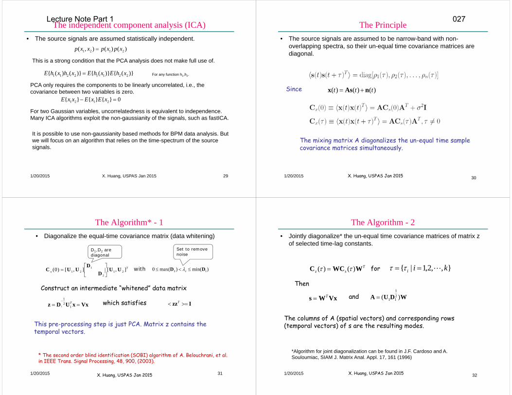
Example of ID field (EPU for MAX-II)

1/19/2015 18

Orbit for1.5 GeV electrons

Planar

Circular

I. Blomqvist


References1. M. Basetti and C. Biscari, Part. Accel. 52, 221 (1996)2. Y. Cai and Y. Nosochkov, SLAC-PUB-11181 (2005)3. K. Brown, SLAC-Report-75 (1982)4. E. Forest and Milutinovic, NIMA 269, 474-482 (1988)5. J. Irwin and C.-x. Wang, Explicit soft fringe maps of a quadrupole, PAC 95 (1995)6. X. Huang, et al, Lattice modeling for SPEAR3, IPAC 20107. Lloyd Smith, Effect of wigglers and undulators on beam dynamics, ESG-Tech-note-24, (1986)8. P. Elleaume, A new approach to the electron beam dynamics in undulators and wigglers, EPAC 92,

p. 661 (1992)9. J. Safranek, et al, Nonlinear dynamcis in a SPEAR wiggler, PRSTAB 5, 010701 (2002)

1/19/2015 19X. Huang, USPAS Jan 2015


1/20/2015 1

Lecture 4: Lattice model calibration and machine optics correction


Hampton, Virginia


Outline• Motivation

– Error sources in real machines.– Correcting the errors improves machine performance.

• Orbit correction• Model calibration with orbit response matrix

– LOCO

• Optics measurement and lattice calibration with turn-by-turn BPM data– Traditional method– MIA and ICA.


Lattice errors in machine• An actual machine always deviates from the ideal model.

– The model makes simplifying assumptions, e.g. hard-edge magnet model.– Systematic and random field errors in actual magnets.– Magnet power supply setpoint errors (e.g., gradient to current conversion)– Errors in power supply regulation.– Magnet hysteresis. – Misalignments.– Malfunctions, human errors, etc.

• Symptoms of errors in the machine– Closed orbit different from design orbit (side effects include optics and

coupling errors due to magnet “feed-down”).– Linear optics and coupling errors.– Degraded nonlinear dynamic performance (poor injection efficiency and

lifetime)


Orbit errors and correction• Sources of orbit errors

– Misalignments– Steering errors from bending magnets

1/20/2015 4

Closed orbit errors (simulated) from a SPEAR3 QF magnet with alignment errors of 100 for both planes (kick angles Δ 64 ) .

Orbit errors from one kick:Δ cosfrom random kicks: Δ ̅2 2 sin



Beam-based alignment• Target of orbit correction: centers of quadrupole magnets.• Determination of quadrupole centers with beam-based alignment

(BBA) measurement.– Principle: when there is an orbit offset through a quadrupole, a change to

quadrupole strength causes orbit shifts. – Method (model independent): For a quadrupole, steer the beam orbit at the

quadrupole with a corrector, at each point change quadrupole strength and measure orbit shift. Fit orbit shifts vs. readings of the nearest BPM to find the position corresponding to quad center.

1/20/2015 5

Quad center


Orbit response matrix and orbit correction• Orbit response: closed orbit shifts due to a kick by an orbit corrector.

• Orbit correction

1/20/2015 6

Horizontal orbit response at BPM induced by a horizontal corrector :, Δ ,Similarly on the vertical plane (correctors may be different from -plane., Δ ,Cross-plane responses (caused by coupling), , , and , ,Overall response matrix ΔΔOr simply Δ .

ΔSingular value decomposition may be used to invert the response matrix with selection or weighting of the singular values.


Optics errors• Error sources

– Quadrupole components (e.g., random errors) from magnets– Horizontal orbit offsets in sextupoles– Effects not accounted for in ideal model (e.g., quadrupole fringe field, errors in edge

focusing model in dipole.)

• Small quadrupole errors accumulate to large optics distortions.

1/20/2015 7

Beta-beat from one quadrupole errorΔ Δ2 sin 2 cos 2 2From random (phase uncorrelated) quadrupole errorsΔ ̅ Δ2 2 sin 2Betatron phase errorΔ Δ Δ ΔTherefore Δ 12 Δ


Optics errors - example

1/20/2015 8

0 50 100 150 200-0.1

-0.05

0

0.05

0.1

s (m)

"-=

-

SPEAR, 99 quads, kl=0.001 m-1

xy

0 200 400 600 800 1000-0.4

-0.2

0

0.2

0.4

s (m)

"-=

-

APS, 400 quads, kl=0.001 m-1

xy

SPEAR3, mean | | 0.54Estimate w/ formula: [0.036, 0.037]mean , ~7m APS,mean | | 0.38

Estimate w/ formula: [0.135, 0.117]mean , ~15.5, 17.9m



Measurement of optics errors• Direct beta function measurement at a quadrupole location

• Measurement with turn-by-turn BPM data with beam in oscillation.– Betatron oscillation amplitude – Betatron phase advances

• Indirect measurement – fit lattice model to data that represent linear optics

– Orbit response matrix

1/20/2015 9

Measure tune shift induced by a small quadrupole strength change:Δ Δ

Difficulty: the actual Δ by a quadrupole current change cannot be accurately determined because of magnet hysteresis.

Closed orbit response data contain both beta function and phase advance information Δ 2 sin cos


Measurement of dispersion function• Changing RF frequency in a storage ring causes beam energy change

and closed orbit shifts.

• Error sources for horizontal dispersion– Focusing errors (quadrupole gradient errors)– Bending errors (distribution of 1/ )

• Error sources of vertical dispersion– Rolls of bend mangets; vertical correctors; vertical orbit offsets in quadrupoles.– Rolls of quadrupoles (skew quads) at dispersive locations.– Vertical orbit offsets in sextupoles at dispersive locations.

1/20/2015 10

/ , /Dispersion measurement is very reliable and accurate. The main uncertainty is from BPM calibration.

1

1 2X. Huang, USPAS Jan 2015

Linear optics from closed orbit (LOCO)• Principle: adjust quadrupole strengths in the lattice model so that the

calculated orbit response matrix agrees with the measured orbit response matrix, i.e., to minimize function

• Effects of BPM gains and roll: what BPMs report is not exactly where the beam is.

• Effects of corrector gain and roll: kicks beam gets are different from what corrector readback report.

1/20/2015 11

Δ Δ,

Note the difference between and accounts for BPM “crunch” (deformation from ideal configuration).

,, , , ,, , ,


• Degeneracy due to BPM and corrector gain ambiguity – an overall BPM calibration scale factor can be canceled with an overall corrector gain scale factor.

– All horizontal BPM gain can be 1.1 larger while all horizontal correctors /1.1smaller, with no change to .

• Dispersion functions are included in fitting (additional terms in definition).

– This helps decouple the BPM and corrector gain as dispersion function measurements do not involve correctors.

• The minimization problem is

1/20/2015 12

, Δ Δ / ,

,where includes all fitting parameters.



Solving a least square problem

1/20/2015 13

rrpp ');()( 22 ii xyyf

Problem: find lattice parameters that minimize the objection function.

General nonlinear least square problem:

);( piii xyyr Residual vectorj

iij p

rJ

Jacobian matrix

Usually it is solved iteratively, at each step, solve for

ppHpppp

pp

)('21)()()( 000

fff

p by minimizing

Leading to condition )()( 00 pp

ppH

f

At the minimum we have 0)(

mf pp

X. Huang, USPAS Jan 2015 1/20/2015 14

pJrr 0with pJJprJprrp ''''2')( 000f

So the solution at each step is given by

0'' rJpJJ Gauss-Newton method

This is equivalent to solve 0rpJ with SVD SVUJ ' USVJ '''

01

02

01 '')'(')'( rUVSrVSUVVSrJJJp

because

(1)

(2)

Numerically approach (1) has a big advantage because SVD of the Jacobian is slow and may be impossible if the matrix size is large (with limited computer memory).


Challenges due to cross-talk between parameters

1/20/2015 15

For LOCO, the Jacobian matrix is often near degenerate, resulting large prediction of Δ , which is unrealistic and potentially impossible to use for optics correction or even updating the model. The near-degeneracy is caused by correlation of the fitting parameters.

0 50 100 150 200 2500

0.2

0.4

0.6

0.8

1

s (m)

,

corr. coef. x /

y/

21

2112 JJ

JJT

Correlation of two parameters

Correlation of adjacent quads in SPEAR3

0 10 20 30 40 50 60 70 80 9010-4

10-2

100

102

Index

Sin

gula

r Val

ues


Fitting LOCO with constraints

1/20/2015 16

A common approach is to cut off the singular values with a threshold. This prohibits the solution to have any component in the sub-space of the parameter space removed by the cut-off and thus limits the accuracy of the solution.

Yet another way to adding constraints or cost functions to the fitting parameters:

This approach limits the stray of the solution in the under-constrained sub-space (formed by directions with small SVs) and allows the solution to have components in it if that is what data demands.

Another common approach is to use a reduced set of fitting parameters (quads). This also will remove a sub-space. However, it would work if the effects of the left-out quads are represented by the fitting quads. (In other words, each left-out quad is highly correlated with some or a combination of fitting quads).

k

kkK

Kw 222

20

2 1

Equivalently, we are requiring Δ 0 with some weight relative to other terms.

0 kK



Effect of the constraints

1/20/2015 17

An illustration of the changes to the convergence path with or without constraints. Solid: no constraints; Dashed: with constraints.

The rms relative change of gradients vs. the residual χ2 for real SPEAR3 data set. Green: no constraints; Blue: with constraints. Point 0 is located at ( 2 10 , 0).


Optics correction with LOCO results• When Δ is found with fitting, make correction to quadrupole setpoint

accordingly to compensate these errors. High precision of optics correction can be achived.

1/20/2015 18

Correction results with Matlab LOCO for SPEAR3


Correction results at ALS

1/20/2015 19(courtesy of James Safranek)

• LOCO fit indicated gradient errors in ALS QD magnets making y distortion.

• Gradient errors subsequently confirmed with current measurements.

• LOCO used to fix y periodicity.

• Operational improvement.


Coupling correction• The off-diagonal blocks of the

response matrix and are due to rolls of BPMs and correctors and coupling in the lattice.

• Fitting skew quadrupoleparameters can uncover equivalent sources of coupling. Compensating these sources (changing skew quad setpoints) can reduce coupling.

• At SPEAR3 coupling can be reduced to 0.05% (vertical emittance 5 pm).

1/20/2015 20

Lifetime, 19 mA, single bunch4.5 hours

1.5 hours

Coupling correction on

Correction off

Life

time



Optics measurement and correction with TBT BPM data• Example of turn by turn data. For TBT BPM data to contain optics

information, beam needs to be excited (kicked or resonantly driven) so that the beam centroid undergoes coherent oscillation.

• Decoupled betatron oscillation

1/20/2015 21

0 500 1000 1500 2000-2

-1

0

1

2

turn

x

SPEAR3

0 500 1000 1500 2000-1.5

-1

-0.5

0

0.5

1

1.5

turny

SPEAR3

0.05 0.1 0.15 0.20

200

400

600

800

SPEAR

FFT

ampl

itude

At BPM , on the -th turn 2 sin 2 2 sin 2 Where , are action variables, , are phase advances.TBT BPM data contain information of beta function and phase advance that are not difficult to extract. How to extract such information consistently, accurately and efficiently?


A method of processing TBT data(1) Obtain the tunes with NAFF or interpolated FFT.(2) Calculate amplitude and phase for each BPM

(3) The measured phase can be used to derive beta function, using model values of beta function and phase advances.

1/20/2015 22

∑ cos 2 , ∑ sin 2 , Then amplitude and phase are

, and cot ,where is the number of turns. Error of phase1 2

P. Castro et al, PAC 93.

cot cotcot cot 1 2 3X. Huang, USPAS Jan 2015

• Disadvantages– Not suited if or data are not a single sinusoidal signal (e.g., with

linear coupling, synchrotron motion or contaminating signals).– Each BPM is treated independently, not benefiting from the fact all

BPMs observe the same oscillations.– Finite number of turns introduces errors to phases since ∑ cos 2 sin 2 0– Need the ideal model to calculate beta function.

• Model independent analysis (MIA) and Independnetcomponent analysis for TBT data processing– Treat all BPM data consistently.– De-couple individual signals from observations. – Reduce noise.

1/20/2015 23X. Huang, USPAS Jan 2015 24

A model of BPM turn-by-turn data• The turn-by-turn beam position signal is a combination of various

source signals.

)()()( ttt nAsx

)()()( tntsatx jj

jiji

Form a matrix of the BPM data

or

For the i’th BPM

A is the mixing matrix

m BPMs and T turns

There are only a few meaningful source signals, such as betatron oscillation and synchrotron oscillation.

1/20/2015 X. Huang, USPAS Jan 2015


Betatron modes via singular value decomposition

25

It has been proven that when the BPM reading contains only one betatron mode, i.e.))(cos()(2)( mmm ttJtx

then there are only two non-trivial SVD eigen-modes TTT vuvuUSVx ss

))(sin()(2)(

),)(cos()(2)(

0

0

tJTtJtv

tJTtJtv

)sin(1

),cos(1

0,

0,

mmm

mmm

Js

u

Js

u

u: spatial vector v: temporal vector

Beta function and betatron phase advance can be calculated from the spatial vector.

)(tan,

,1

m

mm us

us

])()[(1 2,

2, mmm usus

J

U,V are orthogonal matrices,S is a block-diagonal matrix.

Note the constant orbit offsets are always removed for each BPM. This is called “centering”.


What does SVD do?

26

-2 -1 0 1 2-1.5

-1

-0.5

0

0.5

1

1.5

x BPM1

x B

PM3

-2 -1 0 1 2-2

-1

0

1

2

x BPM1

x B

PM2

The BPM data can be viewed as T points in the m-dimensional space. ))(,),(),(()( 21 txtxtxtP m

These points form an hyper-ellipsoid. What SVD does is to identify its principal-axes. This is called principal component analysis (PCA).PCA: with a linear orthogonal transformation to obtain a set of linearly un-correlated components (variables) which holds (successively) the largest variances.

The results in the previous slide states: with only one betatron mode in the BPM data, the hyper-ellipsoid degenerates to an ellipse (2D).

Projection onto (x1, x2) Projection onto (x1, x3)

TTT SSUUxx , The U matrix diagonalize the covariance matrix.


Noise reduction with SVD

27

As the random noises are distributed in all eigen-modes while the signals are concentrated in the leading eigen-modes, noise can be reduced by re-constructing the data after removing the noise-only (with small singular values) modes.

0 20 40 60 80 100 12010-3

10-2

10-1

100

index

SV

The small singular value modes are mostly from noises.

-0.2 -0.15 -0.1 -0.05 0 0.05 0.1 0.150

50

100

150

200

x (mm)

coun

t

before reductionafter reduction

Keep 10 out of 114 modes.

0 10 20 30 40 50 601

2

3

4

5

6 x 10-5

xBPM

before reductionafter reduction

The noise level ( ) is reduced (keeping out of 2 modes) to

mp

n 2


Limitation of the PCA method

X. Huang, USPAS Jan 2015 28

The eigen-modes are determined by the orthogonality and variances (strengths) of the components. If two signals have nearly the same strengths, they will be mixed in the eigen-modes (degeneracy in eigen-analysis). In reality this is common:(1) Horizontal and vertical betatron modes can be mixed. (2) Betatron modes can be mixed with the synchrotron mode. (3) Actual BPM data are often plagued by signal contamination or failing electronics.

0 5 10 15 2010-1

100

101

102

index

SVSPEAR3 data: 8 BPM

0 0.05 0.1 0.15 0.2 0.25 0.3 0.35 0.4 0.45 0.50

200

400

600

800

1000

1200SPEAR3 data: 8 BPM

FFT

ampl

itude

0 50 100 150 200 250 30010-2

10-1

100

101

102

index

SV

APS data: 263 BPMs, horizontal only

0 50 100 150 200 250

10-1

100

101

102

103104

105

index

SV

RHIC data: 130 BPMs

The first mode with real signal is the 7th.

Horizontal BPM only

1/20/2015


The independent component analysis (ICA)• The source signals are assumed statistically independent.


)()(),( 2121 xpxpxxp

This is a strong condition that the PCA analysis does not make full use of.

)}({)}({)}()({ 22112211 xhExhExhxhE For any function h1,h2.

PCA only requires the components to be linearly uncorrelated, i.e., the covariance between two variables is zero.

0}{}{}{ 2121 xExExxE

For two Gaussian variables, uncorrelatedness is equivalent to independence. Many ICA algorithms exploit the non-gaussianity of the signals, such as fastICA.

It is possible to use non-gaussianity based methods for BPM data analysis. But we will focus on an algorithm that relies on the time-spectrum of the source signals.

1/20/2015 X. Huang, USPAS Jan 2015 30

The Principle • The source signals are assumed to be narrow-band with non-

overlapping spectra, so their un-equal time covariance matrices are diagonal.

Since

The mixing matrix A diagonalizes the un-equal time sample covariance matrices simultaneously.

)()()( ttt nAsx

1/20/2015


The Algorithm* - 1• Diagonalize the equal-time covariance matrix (data whitening)

Izz T

Tx ],[],[)0( 21

2

121 UU

DD

UUC

VxxUDz T

121

1

)min()max(0 12 DD cwith

Set to remove noise

D1,D2 are diagonal

Construct an intermediate “whitened” data matrix

which satisfies

This pre-processing step is just PCA. Matrix z contains the temporal vectors.

* The second order blind identification (SOBI) algorithm of A. Belouchrani, et al. in IEEE Trans. Signal Processing, 48, 900, (2003).

1/20/2015 X. Huang, USPAS Jan 2015 32

The Algorithm - 2• Jointly diagonalize* the un-equal time covariance matrices of matrix z

of selected time-lag constants.

Tsz WWCC )()( },,2,1|{ kii

WDUA )( 21

11VxWs T

Then

and

for

The columns of A (spatial vectors) and corresponding rows (temporal vectors) of s are the resulting modes.

*Algorithm for joint diagonalization can be found in J.F. Cardoso and A. Souloumiac, SIAM J. Matrix Anal. Appl. 17, 161 (1996)

1/20/2015



Linear Lattice Functions Measurements• There are two betatron modes because each BPM sees different

phase.

• There is one synchrotron mode.

2211 sAsAx bb

)( 22

21 bb AAa

2

11tanb

b

AA

The betatron component

Beta function and phase advance

ll sAx

lx bAD bsl

The synchrotron componentDispersion function and momentum deviation

1/20/2015 X. Huang, USPAS Jan 201534

Example: de-coupling

A Plus Mode

A Minus Mode

FFT spectra of raw horizontal and vertical BPM signals at section L1. Both BPMs see a mixture of the “plus” mode and “minus” mode.

The ICA method can de-couple the normal modes in presence of linear coupling.

1/20/2015

Comparison of phase measurement results

1/20/2015 35

0 10 20 30 40 50 60 70 80 90-0.01

-0.005

0

0.005

0.01

Phase X

p

hase

X

Phase: Measured - actual

0 5 10 15 20 25 30 35 40-8

-6

-4

-2

0

2x 10-3

Phase Y

p

hase

Y

noise freewith noisequad err actualnoise+quad errorica,w/ noiseica, qerr w/noisi

Cases: 1. Castro method noise free. 2. Castro noise with noise.3. Actual phase error due to a quadrupole error.4. Castro method w/ quad error and noise.5. ICA with noise. 6. ICA w quad error and noise.


Lattice calibration with ICA • The measured beta functions, phase advances and

dispersion functions can be used to fit lattice model by comparing them to calculated values.

• This method can also be extended to fit coupling.

1/20/2015 36X. Huang, USPAS Jan 2015


References1. J. Safranek, NIMA, 388, 27 (1997)2. X. Huang, et al, ICFA beam dynamics newsletter, 44, (2007).3. G. Portmann, et al, ICFA beam dynamics newsletter, 44, (2007).4. P. Castro, et al, PAC 93 (1993)5. Chun-xi Wang, et al. PRSTAB 6, 104001 (2003).6. X. Huang, et al, PRSTAB, 8, 064001, (2005)

1/20/2015 37X. Huang, USPAS Jan 2015


1/20/2015 1

Lecture 5: Optimization of accelerators in simulation and experiments

X. HuangUSPAS, Jan 2015

X. Huang, USPAS Jan. 2015

Outline• Optimization in simulation

– General considerations– Optimization algorithms– Applications of MOGA– Applications of MOPSO

• Optimization in experiments– General considerations of online optimization– Problems with traditional methods for online application.– The RCDS method and application

1/20/2015 2X. Huang, USPAS Jan. 2015

Considerations of optimization in simulation• Single objective or multiple objectives?

– When there are multiple conflicting objectives, consider using multi-objective algorithms.

• The decision variables (knobs)– The number of decision variables – size of the problem

• Evaluation of objective function(s)– Slow or fast?– Numerical noise

• The constraints– Parameter range– Cost functions

• Complexity of parameter space– Smoothness of function– Local minima

1/20/2015 3X. Huang, USPAS Jan. 2015

Choice of algorithms• Traditional algorithms

– Gradient based algorithms: Gauss-Newton, quasi-GN, Levenberg-Marquadt

– Iterative line search: Powell’s method– Downhill simplex method– More …– comments: single objective function; smooth function; result may

depend on initial condition (local minima); small scale problems; converge fast.

• Stochastic algorithms– Simulated annealing– Evolutionary algorithms– Particle swarm algorithms– …– Features: complex parameter space; can work with multi-objective

problems; large scale problems; less efficient. 1/20/2015 4X. Huang, USPAS Jan. 2015


5

Comparison of solutions for multi-objective optimzation


Problem: minimize , 1,2, … , with parameter ranges ∈ ,Comparison of two solutions (definition of domination): Solution dominates solution if for all 1,2, … , , we have and for at least one objective ′, .

Pareto front: the set of all solutions in the search space that are non-dominated by any solutions.

Goal of multi-objective optimization is obtain the Pareto front for further analysis.

1/20/2015

A multi-objective genetic algorithm: NSGA-II• NSGA (non-dominated sorting genetic algorithm)–II

1/20/2015 6X. Huang, USPAS Jan. 2015

K. Deb, IEEE Transtions On Evolutionary Computation Vol 6, No 2,April 2002

Selection (of parents)Crossover Mutation

Application of NSGA-II: injector optimization (Cornell )

1/20/2015 7

Decision variables:

I. Bazarov, PRSTAB 8, 034202, (2005) X. Huang, USPAS Jan. 2015

Other examples

1/20/2015 8

M. Borland

L. Yang

Examples of application to nonlinear dynamics optimization



Multi-objective particle swarm optimization

1/20/2015 9

X. Pang

position (parameter vector) of particle at iteration .velocity (increment) of particle at iteration .

Control parameters: 0.4, 1., are random within 0, 1 or fixed values.

Updating particle population in an iteration

MOPSO can also include mutation operation.

MOPSO also manipulates a population of solutions over many iterations with random operations.

X. Pang, L.J. Rybarcyk, NIMA 741 (2014)


Comparison of MOGA and MOPSO in a study

1/20/2015 10

Optimizing transmission and matching to the DTL of the LANSCE linac at LANL:Objectives: beam loss and mismatch factorsKnobs: four quadrupoles in the transport line prior to DTL.


The need of online optimization

1/20/2015 11

• The general need of online optimization.– Lack of diagnostics (that monitor the sub-systems)

• Injection steering and transport line optics.– Target values of monitors not established (or drifting)

• Initial commissioning.– Lack of deterministic procedure to go to target values.

• Nonlinear beam dynamics in storage rings.

• Manual tuning – online optimization of a complex system.– We want automate the tuning process with efficient algorithms.

• Difficulty in automated tuning– Automated tuning is basically optimization of noisy functions of multiple

variables. – Traditional optimization algorithms are usually for smooth functions.


Considerations of online optimization

1/20/2015 12

• High efficiency – get to the optimum fast– Online evaluation of the objective is usually slow.– Machine study time is usually limited (and expensive). – Efficiency may be measured by the number of function evaluations.

• Robustness – surviving noise, outliers and machine failures• Live status reporting during optimization. • Traditional algorithms are usually not suitable for noisy online

problems.• An algorithm designed for online optimization

– Robust conjugate direction method (RCDS) – A combination of Powell’s method and a new noise resistant line optimizer.



Powell’s method*Powell’s method has two components:1. A procedure to update the direction set to make it a conjugate set.2. A line optimizer that looks for the minimum along each direction.

Directions u, v are conjugate if: 0vHu where the Hessian matrix is defined

jiij xx

fH

2

Searching along mutually conjugate directions is more efficient since a scan along one direction doesn’t ruin previous results on other directions.

Line optimizer:

Inverse parabolic interpolation (figure from N.R.)

Another choice is golden section search (bisection).

Both line optimization approaches are sensitive to noise – one wrong decision (due to noise) leads the search away from the real minimum.

*M.J.D. Powell, Computer Journal 7 (2) 1965 155

131/20/2015 X. Huang, USPAS Jan. 2015

The robust line optimizer

Step 1: bracketing the minimum with noise considered. Step 2: Fill in empty space in the bracket with solutions and perform quadratic fitting. Remove any outlier and fit again. Find the minimum from the fitted curve.

Global sampling within the bracket helps reducing the noise effect.

RCDS is Powell’s conjugate method* + the new robust line optimizer. *however, since the online run time is usually short, it is important to provide good an initial conjugate direction set which may be calculated with a model.

-0.06 -0.04 -0.02 0 0.02-0.9

-0.8

-0.7

-0.6

-0.5

obje

ctiv

e

bracketingfill-infittednew minimum

Initial solution

141/20/2015 X. Huang, USPAS Jan. 2015

A simulation study: coupling correction for SPEAR3

1/20/2015 15

– Using calculated beam loss rate as the objective function.– Noise is generated in the objective function by adding random

noise to beam current values (used for loss rate calculation). – There are 13 coupling correction skew quads in SPEAR3. – Initial conjugate direction set is from SVD of the Jacobian matrix of

orbit response matrix w.r.t. skew quads– With

• 500 mA beam current with 1% random variation. On top of that a DCCT noise with sigma = 0.003 mA. The beam loss rate noise evaluated from 6-s duration is 0.06 mA/min.

• 40 hour gas lifetime; 10 hour Touschek lifetime with 0.2% coupling. • The coupling ratio with all 13 skew quads off is 0.9% (with simulated

error), corresponding to a loss rate of 0.6 mA/min.


Comparison of performance (best of 6-s cases)

0 500 1000 1500 2000-3

-2.5

-2

-1.5

-1

-0.5

obje

ctiv

e (m

A/m

in)

count

RCDSsimplexPowellIMATMOGA

0 500 1000 1500 200010-4

10-3

10-2

coup

ling

ratio

count

RCDSsimplexPowellIMATMOGA

The IMAT method uses the same RCDS line optimizer, but keep the direction set of unit vectors (not conjugate).

Clearly, (1) the line optimizer is robust against noise.(2) Searching with a conjugate direction set is much more efficient.

Note that the direction set has been updated only about 8 times after 500 evaluations (out of 13 directions). So the high efficiency of RCDS is mostly from the original direction set.

161/20/2015 X. Huang, USPAS Jan. 2015


Experiment: coupling correction with loss rate

0 2 4 6 8 10 12 14-20

-15

-10

-5

0

5

10

15

skew quad index

curre

nt (A

)

run 2-27-2013run 3-26-2013run 4-23-2013LOCO 2-13-2013LOCO 4-23-2013

0 50 100 150 200 250-2

-1.5

-1

-0.5

0

-loss

rate

(mA

/min

)

count

2-27-2013

allbest

0 100 200 300 400 500 600-2

-1.5

-1

-0.5

0

count

-loss

rate

(mA

/min

)

3-26-2013

allbest

Beam loss rate is measured by monitoring the beam current change on 6-second interval (no fitting). Noise sigma 0.04 mA/min. Data were taken at 500 mA with 5-min top-off.

Initially setting all 13 skew quads off. Loss rate at about 0.4 mA/min. Final loss rate at about 1.75 mA/min. At 500 mA, the best solution had a lifetime of 4.6 hrs. This was better than the LOCO correction (5.2 hrs)

Best result with RCDS is loss rate >2.0 mA/min and 500 mA lifetime 4.2 hrs.

171/20/2015 X. Huang, USPAS Jan. 2015

Experiment: kicker bump matchingParameters: Adjusting pulse amplitude, pulse width and timing delay of K1 and K3 (with K2 fixed) and two skew quads for vertical plane (This is the setup by James for kicker bump matching), 8 parameters total.

Objective: sum of rms(x) and rms(y) of turn-by-turn orbit (for 30~300 turns).

0 20 40 60 80 100 1200

50

100

150

200

250

count

obje

ctiv

e (m

icro

n)

3-25-2013, LE lattice

0 50 100 150 200 250 300 350 4000

200

400

600

800

1000

1200

1400

obje

ctiv

e (m

icro

n)

count

3-26-2013, LA20 lattice

First time of getting kicker bump for low alpha lattice matched.

181/20/2015 X. Huang, USPAS Jan. 2015

References:(1). W. H. Press, et al, Numerical Recipe, Cambridge University Press, 3rd Ed. (2007)(2). K. Deb, IEEE Transtions On Evolutionary Computation Vol 6, No 2,April 2002 (3) I. Bazarov, PRSTAB 8, 034202, (2005) (4) X. Pang, L.J. Rybarcyk, NIMA 741 (2014)(5) X. Huang, et al, NIMA 726 (2013)

1/20/2015 19X. Huang, USPAS Jan. 2015


Documents

Outline Coordinate system for beam motion - IU Bphysics.indiana.edu/~shylee/p571/AAP_part_1.pdfHamiltonian 1/19/2015 5 After a series of canonical transformations, new Hamiltonian