OUT-OF-PLANE VIBRATIONS OF PLANAR CURVED …library.iyte.edu.tr/tezler/master/makinamuh/T001031.pdf · OUT-OF-PLANE VIBRATIONS OF PLANAR CURVED BEAMS HAVING VARIABLE CURVATURE AND

OUT-OF-PLANE VIBRATIONS OF PLANAR

CURVED BEAMS HAVING VARIABLE

CURVATURE AND CROSS-SECTION

A Thesis Submitted to

the Graduate School of Engineering and Sciences of

Ġzmir Institute of Technology

in Partial Fulfillment of the Requirements for the Degree of

MASTER OF SCIENCE

in Mechanical Engineering

by

Kaan KAYGISIZ

June 2012

ĠZMĠR

We approve the thesis of Kaan KAYGISIZ 12 points

Examining Committee Members:

________________________________

Prof. Dr. Bülent YARDIMOĞLU

Department of Mechanical Engineering,


________________________________

Assoc. Prof. Dr. Moghtada MOBEDI



________________________________

Assist. Prof. Dr. Levent AYDIN


Ġzmir Katip Çelebi University

29 June 2012

______________________________

Prof. Dr. Bülent YARDIMOĞLU

Supervisor, Department of Mechanical Engineering,


______________________________ ______________________________

Prof. Dr. Metin TANOĞLU Prof. Dr. R. Tuğrul SENGER

Head of the Department of Dean of the Graduate School

Mechanical Engineering of Engineering and Sciences

ACKNOWLEDGEMENTS

Apart from the efforts of me, the success of any project depends largely on the

encouragement and guidelines of many others. I take this opportunity to express my

gratitude to the people who have been instrumental in the successful completion of this

study.

First and foremost, I would like to thank to my advisor of this thesis, Prof. Dr.

Bülent YARDIMOĞLU who was abundantly helpful and offered invaluable assistance,

support and guidance. Without his encouragement and guidance this study would not

have concluded.

I also wish to express my appreciations to my friends for keeping me up. I

admire the patience of my housemate Osman Burak AġIK. Besides, I am indebted to

Yusuf DĠLER, Sedat SAVAġ and Ġsmail AKÇOK for their supports throughout the hard

times of my life.

Finally, yet importantly, I would like to express my heartfelt thanks to my

beloved family for their blessings, for their helps and wishes for the successful

completion of this thesis. Special thanks go to Ceylin & Ceren, who are the newly

quests of KĠLMEN and ÖZTÜRK families, for reminding us the value of life.

iv

ABSTRACT

OUT-OF-PLANE VIBRATIONS OF PLANAR CURVED BEAMS

HAVING VARIABLE CURVATURE AND CROSS-SECTION

In this study, out of plane vibration characteristics of curved beams having

variable curvatures and cross-sections are studied by FDM (Finite Difference Method).

The effects of curvature and cross-section of the curved beam on natural frequencies are

investigated for the curved beams having; variable curvature & constant cross-section

and variable curvature & variable cross-section. Mathematical model of the present

problem is based on the coupled differential eigenvalue problem with variable

coefficients. Numerical solutions of the problem in this study are obtained by the

computer program developed in Mathematica. The accuracy of the present results

obtained from the developed program is evaluated by comparing with FEM (Finite

Element Method) results found from solid model created in ANSYS. Good agreement is

obtained in the comparisons of the present results with other results. All results are

presented in tabular and graphical forms.

v

ÖZET

DEĞĠġKEN EĞRĠLĠK VE KESĠTE SAHĠP DÜZLEMSEL EĞRĠ

ÇUBUKLARIN DÜZLEM DIġI TĠTREġĠMLERĠ

Bu çalıĢmada, değiĢken eğrilik yarıçapı ve kesit alanına sahip eğri çubukların

düzlem dıĢı titreĢim karakteristikleri Sonlu Farklar Yöntemi ile incelenmiĢtir. Eğri

çubuğun eğriliğinin ve kesitinin doğal frekanslara etkileri; değiĢken eğrilik-sabit kesit

ve değiĢken eğrilik-değiĢken kesit durumları için araĢtırılmıĢtır. Mevcut problemin

matematiksel modeli değiĢken katsayılı bağlaĢık diferansiyel özdeğer problemine

dayanmaktadır. Bu çalıĢmadaki problemin sayısal çözümü Mathematica’da geliĢtirilmiĢ

bilgisayar programı ile elde edilmiĢtir. GeliĢtirilen programdan elde edilen çözümlerin

doğruluğu ANSYS de oluĢturulan katı modelden bulunan Sonlu Elemanlar Metodu

sonuçları ile karĢılaĢtırılarak değerlendirilmiĢtir. Mevcut sonuçların diğer sonuçlar ile

karĢılaĢtırılmasından iyi uyum elde edilmiĢtir. Tüm sonuçlar tablolar ve grafikler olarak

sunulmuĢtur.

vi

TABLE OF CONTENTS

LIST OF FIGURES ..................................................................................................... vii

LIST OF TABLES ....................................................................................................... viii

LIST OF SYMBOLS ................................................................................................... ix

CHAPTER. 1. GENERAL INTRODUCTION ........................................................... 1

CHAPTER.2. DIFFERENTIAL EQUATIONS AND THEIR SOLUTIONS ............ 7

2.1. Introduction ...................................................................................... 7

2.2. Description of the Problem .............................................................. 7

2.3. Geometry of Curved Beam .............................................................. 8

2.4. Derivation of the Equations of Motion ............................................ 10

2.4.1. Newtonian Method .................................................................... 11

2.4.2. Hamilton’s Method .................................................................... 13

2.5. Natural Frequencies by Finite Difference Method .......................... 16

CHAPTER.3. NUMERICAL RESULTS AND DISCUSSION .................................. 18

3.1. Introduction ...................................................................................... 18

3.2. Comparisons and Applications for Variable Curvature and

Constant Cross-Section ................................................................... 18

3.3. Applications for Variable Curvature and Cross-Section ................. 23

CHAPTER 4. CONCLUSIONS .................................................................................. 32

REFERENCES ............................................................................................................ 33

vii

LIST OF FIGURES

Figure Page

Figure 2.1. Parameters of catenary beam ..................................................................... 8

Figure 2.2. A planar curved beam with variable curvature and cross section ............. 10

Figure 2.3. A curved beam with internal forces and moments .................................... 11

Figure 2.4. A domain divided into six sub domains for approximation ...................... 16

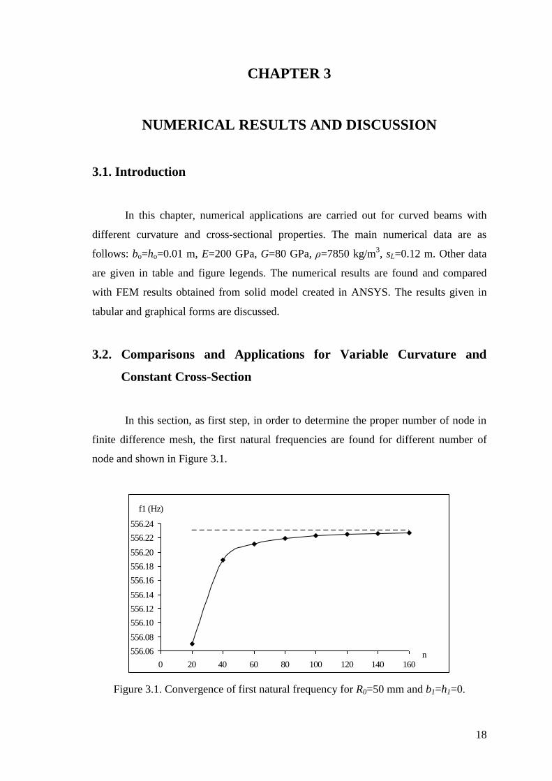
Figure 3.1. Convergence of first natural frequency for R0=50 mm and b1=h1=0.........18

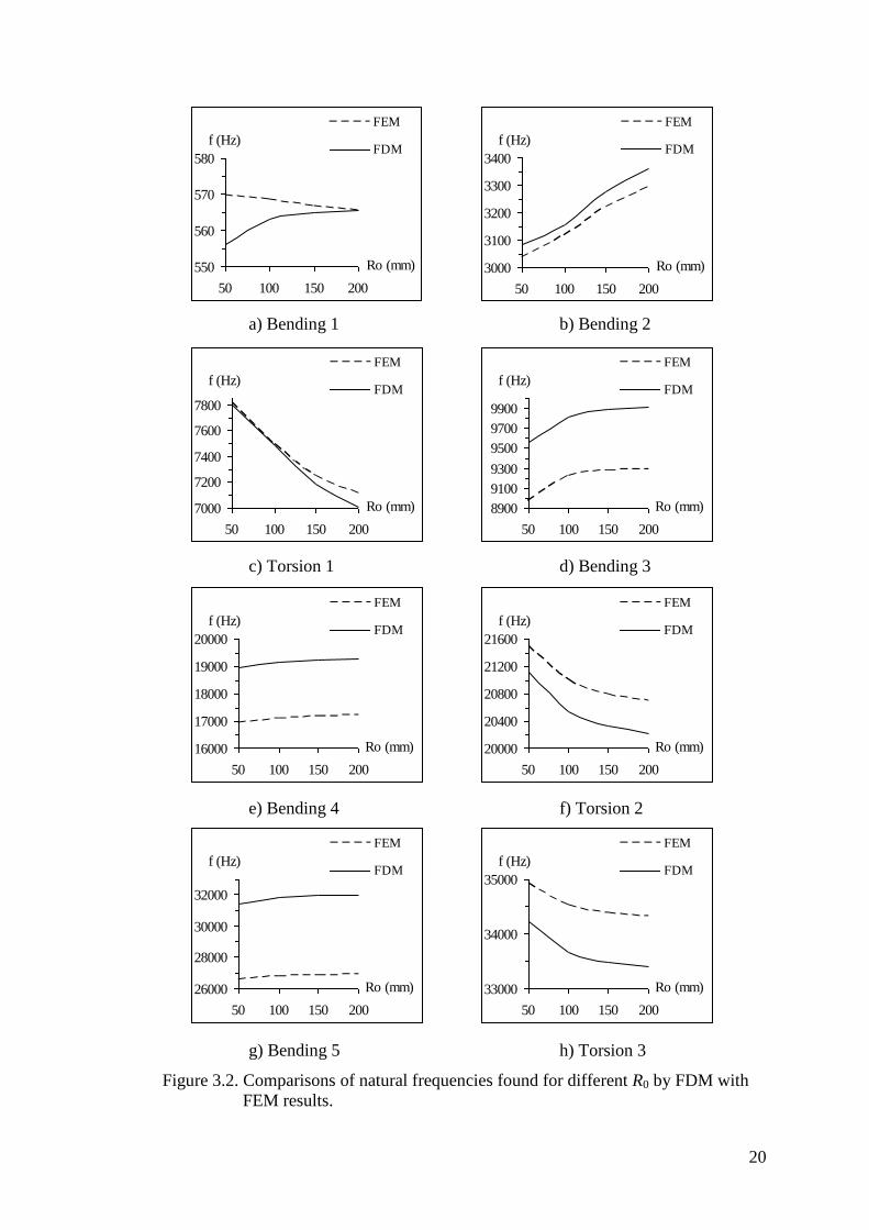
Figure 3.2. Comparisons of natural frequencies found for different R0 by FDM

with FEM results.... ................................................................................... 20

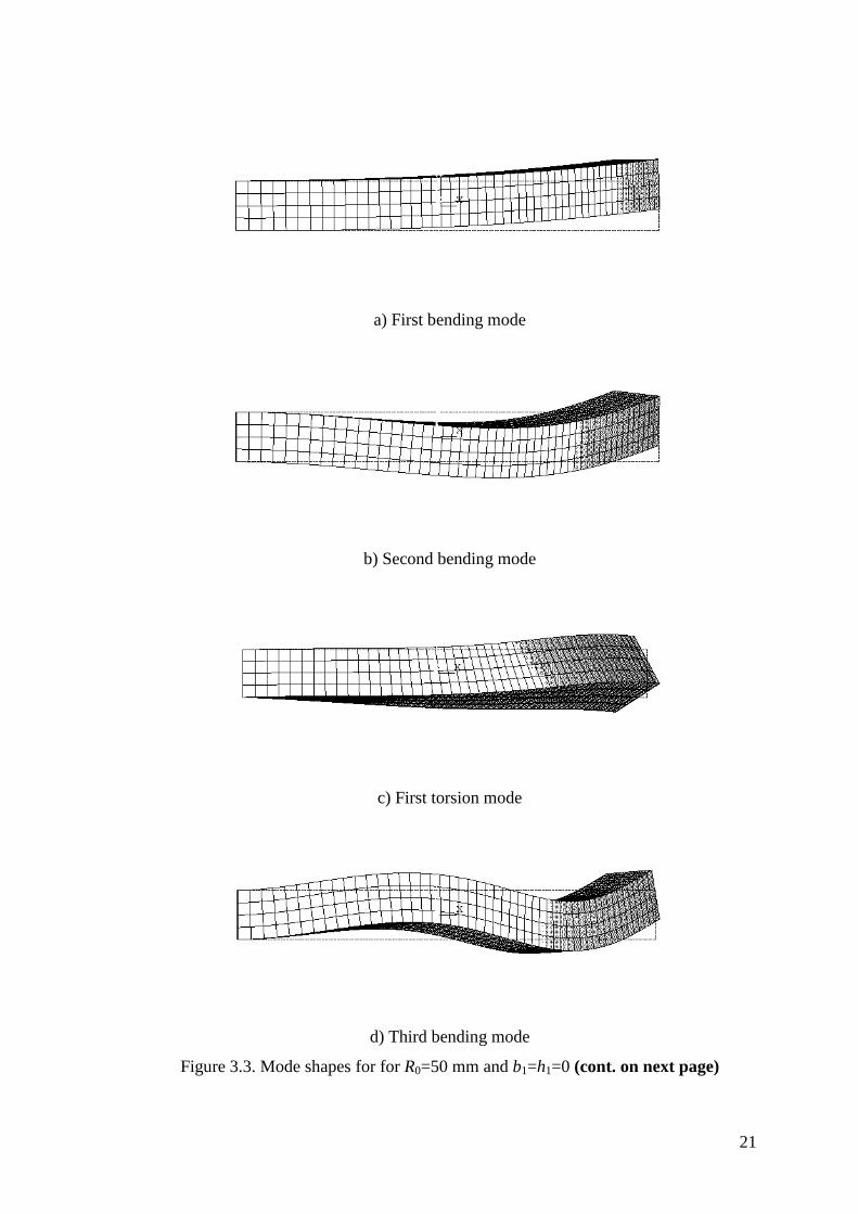
Figure 3.3. Mode shapes for for R0=50 mm and b1=h1=0... ........................................ 21

Figure 3.4. Natural frequencies for b1=h1=2/120... ...................................................... 25

Figure 3.5. Natural frequencies for b1=h1=4/120.. ....................................................... 26

Figure 3.6. Natural frequencies for b1=h1=6/120.. ....................................................... 27

Figure 3.7. Natural frequencies for different b1=h1.. ................................................... 28

viii

LIST OF TABLES

Table Page

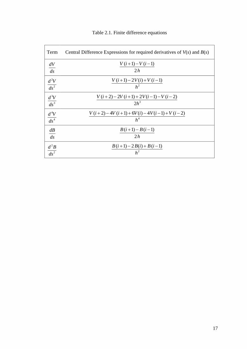
Table 2.1. Finite difference equations ......................................................................... 17

Table 3.1. Comparison of natural frequencies found for different R0 by FDM

with FEM results (b1=h1=0) ........................................................................ 19

Table 3.2. Effects of parameter R0 on natural frequencies for b1=h1=2/120 ............... 23



ix

LIST OF SYMBOLS

A(s) cross-sectional area of the beam

b(s) breadth function of the beam

b0 breadth of the beam at root cross-section

b1 breadth parameter

B(s) angular displacement about z axis as function of s

Cβ the ratio of breadth/depth

E modulus of elasticity

f natural frequency

Fy external force in y direction

G shear modulus

h(s) depth function of the beam

h0 depth of the beam at root cross-section

h1 depth parameter

i mass polar moment of inertia per unit length

Ixx area moment of inertia of the cross-section about xx axis

J(s) torsional constant of cross-section

m mass per unit length of the beam

Mx, Mz bending and twisting moments

Nz internal force along z axis

R0 radius parameter of the catenary curve

s arc length of the curve

sL length of the curve

T kinetic energy

Tz external twisting moment about z axis

x co-ordinate axis

v(s,t) displacement in y direction

V elastic strain energy

V(s) displacement in y direction as function of s

Vy shear force in y direction

α, αr slope of the curve at any point and point r

β(s,t) angular displacement about z axis

x

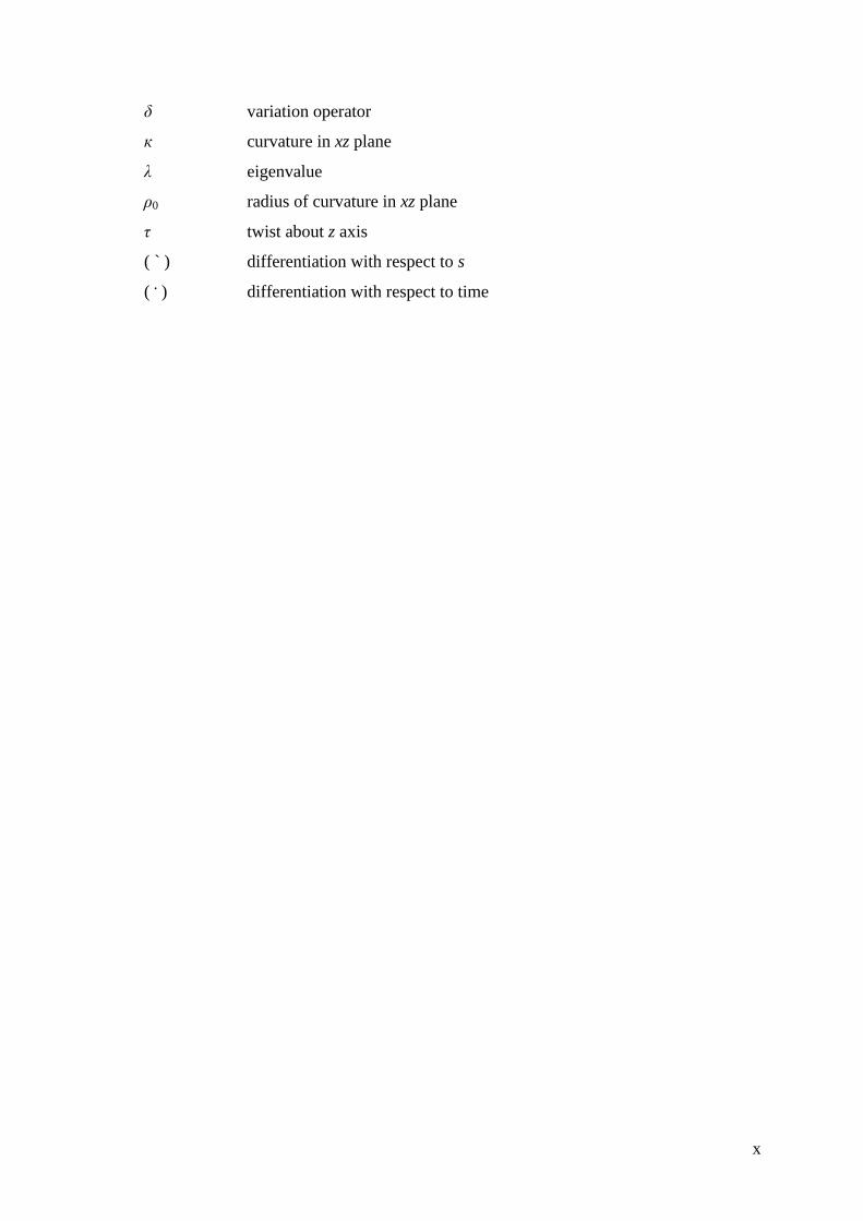
δ variation operator

к curvature in xz plane

λ eigenvalue

ρ0 radius of curvature in xz plane

τ twist about z axis

( ` ) differentiation with respect to s

( . ) differentiation with respect to time

1

CHAPTER 1

GENERAL INTRODUCTION

Vibration is the motion of a particle, system of particles or continuous elastic

body displaced from a position of equilibrium. In other words, vibration is the study for

dynamics of elastic bodies. Vibrations are generally undesired motions for most of the

machines and structures. They cause higher stresses, energy loses, increased bear loads,

induced fatigue, wear of machine parts, damage to machines and buildings and

discomfort to human beings. On the other hand, vibrations have a vital importance for

humans if you think about;

Beating of heart,

Breathing - Oscillation of lungs,

Walking - Oscillation of legs and hands,

Shivering - Oscillation of body in extreme cold,

Hearing - Ear receives vibrations to transmit message to brain,

Speaking - Vocal chords vibrates to make sound.

Curved beam structures have been used in many engineering applications since

the nineteenth century. The utilization of these structures can be mostly found out in the

mechanical, civil, aerospace engineerings and various fields. These applications can be

listed for mechanical engineering as follows: spring design, brake shoes within drum

brakes, tire dynamics, circumferential stiffeners for shells, turbo machinery blades, in

the piping systems of chemical plants, thermal power plants. Also other engineering

applications can be found such as: curved girder bridges, design of arch bridges,

highway construction, long span roof structures, curved wires in missile-guidance

floated gyroscopes, wings of an airplane, propellers of an helicopter; and earthquake

resistant structures. It is really necessary to have a sound knowledge of vibrations for a

design engineer.

Curved beams can be classified depending on their geometrical properties as;

in the shape of a space curve or a plane curve,

constant or variable curvature,

constant or variable cross section.

2

In general, the out-of-plane and the in-plane vibrations of curved beams are

coupled. However, if the cross-section of the curved beam is uniform and doubly

symmetric, then the out-of-plane and the in-plane vibrations are independent (Ojalvo

1962).

Many investigators have been studied out-of-plane vibrations of the curved

beams because of the wide usage of curved beams and until now, insignificant

researches have been performed for variable curvatures and cross-sections. Some of

those researches are introduced in the next paragraphs with the inclusion of their various

methods.

Volterra and Morell (1961) used the Rayleigh-Ritz method to determine the

lowest natural frequencies of elastic arcs with clamped ends. They managed to

formulate the relationships for the length and the radius of curvature of a circle, a

cycloid, a catenary and a parabola.

Chang and Volterra (1969) developed an extended method based on the

differential operator theory to determine the upper and the lower bounds of the first four

natural frequencies of simply-supported arcs with central lines in the forms of circles,

cycloids, catenaries and parabolas. The numerical values of the frequencies are

compared with the results obtained by the Rayleigh-Ritz.

Wang (1975) studied the analysis of the lowest natural frequency of the out-of-

plane vibration for a clamped elliptic arc of constant section. The Rayleigh-Ritz method

is employed to obtain the frequency equation and the numerical results are presented in

the form of curves. The effects of the opening angle on the natural frequencies of the arc

are shown in these curves.

Takahashi and Suzuki (1977) studied the vibrations of an uniform bar, of which

the center line is an arc of ellipse and which vibrates perpendicularly to the plane of

center line, neglecting the rotary inertia and the deformation due to shear. From the

Lagrangion of the bar, equation of motion and the boundary conditions are obtained. By

integrating the curvature along center line a new independent variable introduced to

simplify these equations and boundary conditions. The solution was found out as a form

of power series.

Suzuki et al. (1978) used the Rayleigh-Ritz and Lehmann-Maehly methods to

determine frequencies and mode shapes of various curved bars with clamped ends. At

the same time, they carried out numerical calculations about symmetric ellipse, sine

3

catenary, hyperbola, parabola and cycloid arcs. They obtained a common tendency for

the vibrations of curved bars.

Irie et al. (1980) presented an analysis of the steady state out-of-plane vibration

of a free-clamped Timoshenko beam with internal damping by using the transfer matrix

approach. The equations of the beam are written in a matrix differential equation of first

order by use of this method. The method is applied to free-clamped non-uniform beams

with circular, elliptical, catenary and parabolical neutral axes. The elements of the

matrix are determined by numerical integration, thus from the matrix and the boundary

conditions, all the other variables are determined.

Suzuki and Takahashi (1981) presented a method for a free out-of-plane

vibrations of a plane curved bar including the effects of the bending, the torsion, the

shear deformation and the rotatory inertia of bar. Timoshenko’s beam theory is used to

derive the basic equations. First, the Lagrangian of vibration of a curved bar is obtained

and the equations of vibration and the boundary conditions are determined. Then, the

equations are solved exactly by series solution. Natural frequencies and mode shapes for

symmetric catenary, parabola and cycloid curved bars with clamped ends are obtained.

The numerical results with this theory are compared with the ones by the classical

theory. A good agreement is reached and the effects of the shear deformation and the

rotator inertia are clarified.

Suzuki et al. (1983) used classical theory for the out-of-plane free vibrations of a

plane curved bar with an arbitrary varying cross-section. The equations and the

boundary conditions are determined from the Lagrangian of the bar. Equations are

solved exactly in series solution. The natural frequencies and the mode shapes of an

elliptic arc bars with both clamped ends and both simply supported ends are obtained.

Kawakami et al. (1995) presented a method for the free vibration analysis for

both the in-plane and the out-of-plane cases of horizontally curved beams with arbitrary

shapes and variable cross-sections. Firstly, the fundamental equations of a curved beam

are transformed into integral equations and the discrete Green functions are obtained by

approximate solution of these equations. Secondly, according to the integral theorem,

the fundamental equations transformed into equivalent boundary integral equations.

Finally, the eigenvalues for free vibration are obtained by applying the Green function

and using the numerical integration. Numerical results are compared with those

obtained by a FEM and the effectiveness of the proposed method is confirmed.

4

Huang and Chang (1998) presented an extended methodology for analyzing the

out-of-plane dynamic responses or arches which was used to solve in-plane ones before.

An exact solution is formulated for the transformed governing equations in the Laplace

transform domain. Key elements for the solution such as dynamic stiffness matrix and

equivalent nodal loading vector for a curved bar are also formulated. The analytical

solution in the Laplace domain is obtained by using the Frobenius method. The results

for the displacement component and the stress resultants are given to show the accuracy

of this method. The most important advantage of this method is providing accurate

dynamic responses both for the displacement components and for the higher derivatives

of displacement without any difficulties.

Huang et al. (2000) investigated the linear out-of-plane dynamic responses of

planar curved beams with arbitrary shapes and cross-sections including the effects of

shear deformation and rotary inertia. Frobenius method is used to develop a series

solution for curved beams in terms of polynomials. The exact solution for the out-of-

plane free vibration of a curved beam is established by transforming the solution in the

Laplace domain into the frequency domain. This solution is not limited with symmetry;

both symmetric and anti-symmetric modes are formulated together. Accurate results can

be obtained with the help of Laplace transform and an analytical solution in the Laplace

domain is concluded in higher accuracy for stress resultants. A convergence study is

also presented to demonstrate the validity o f proposed solution.

Lee and Chao (2000) derived the governing equations for the out-of-plane

vibrations of a curved non-uniform beam of constant radius via Hamilton’s principle. A

non-uniform beam with double symmetric cross-section situation is considered. The

thickness of the beam assumed as so small in comparison with the radius of the beam.

Thus, the shear deformation, the rotary inertia and the warping effects are not taken into

account. By introducing two physical parameters, the analysis is simplified and it is

found that the torsional displacement and its derivative can be explicitly expressed in

terms of the flexural displacement. The two coupled governing characteristic

differential equation are decoupled and reduced to one sixth-order ordinary differential

with variable coefficients in the out-of-plane flexural displacement. Exact solutions for

the out-of-plane vibrations of non-uniform curved beams are obtained. The study for a

curved non-uniform beam is successfully revealed with the help of explicit relations.

The influence of taper ratio, center angle and arc length on the first two natural

frequencies of the beam is also studied.

5

Kim et al. (2003) presented an improved energy formulation for spatially

coupled free vibration and buckling of non-symmetric thin-walled curved beams with

variable curvatures. By introducing the displacement field and considering the effects of

variable curvatures, the total potential energy of non-circular curved beam is derived

and then a beam element for Finite Element Analysis is developed. Numerical solutions

are illustrated to show the accuracy and the validity of this element. The influences of

the arch rise to span length ratio on spatial vibrations and buckling behaviors of non-

circular beams with the parabolic and elliptic shapes are also investigated.

Tüfekçi and Doğruer (2006) aimed to give the exact solution to the governing

equations of the out-of-plane deformation of an arch of general geometry and also

exhibit the advantages of the solution by using the initial value method considering the

shear deformation effect. The stress resultants and displacements throughout the beam

are found with the help of initial values of these parameters. The main advantage of this

method is that the higher degree of statically indeterminacy does not add any difficulty

to the solution. The examples in the literature are also solved and the results are

compared with each others.

Lee at al. (2008) derived the governing differential equations out-of-plane free

vibrations of the elastic, horizontally curved beams with variable curvatures and solved

numerically to obtain natural frequencies and mode shapes for parabolic, sinusoidal and

elliptic beams with hinged-hinged, hinged-clamped and clamped-clamped end

constraints. The effects of the shear deformation, rotatory and torsional inertias are

considered whereas the warping of the cross-section is excluded. Non-dimensional

equations of the stress resultants are formulated to present the mode shapes and

deformations. Experimental methods are also described for measuring the free vibration

frequencies for parabolic beams, which agree well with those predicted by theory.

In spite of the fact that, there is no considerable amount of the researches, so the

vibration characteristic is seemed to be an interesting and a worth studying subject since

the variety and the complexity of the effects of the parameters are taken into account.

Therefore, in this study, the effects of variable radius of curvature and cross-section on

vibration characteristics of curved beams are studied. Finite Difference Method is used

to reduce to differential eigenvalue problem to discrete eigenvalue problem to solve

numerically. A symbolic computer program is developed in Mathematica to determine

the eigenvalues. Using the developed program, natural frequencies are obtained and the

effects of parameters such as variable radius of curvature and cross-section are found.

6

The accuracy and numerical precision of the developed program are evaluated

by using the finite element model results found from the solid model created and solved

in ANSYS. A very good agreement is reached in the comparisons of the present results

with FEM results. The effects of cross-section and curvature variation parameters are

given in tabular and graphical form.

7

CHAPTER 2

DIFFERENTIAL EQUATIONS AND THEIR SOLUTIONS

2.1. Introduction

In this chapter, all the necessary information to identify the problem is given.

The geometry of the beam is given and the radius of the curvature is expressed in

desired form. Newtonian method and Hamilton’s principle are presented which are used

to derive the equation of motions. Boundary conditions are listed for different types of

end conditions: clamped, pinned and free.

The governing differential equations of motions for free vibrations which are

derived from the Hamilton’s principle based on the energy equations are introduced. By

using the separation of variable method, the problem is transformed into one

dimensional eigenvalue problem with variable coefficients.

A numerical approach is needed to solve this eigenvalue since the differential

equations having variable coefficients are analytically unsolvable in most cases. The

differential eigenvalue problem is reduced to discrete eigenvalue problem by using

Finite Difference Method. Finally, discrete eigenvalue problem regarding the natural

frequencies and the mode shapes is introduced as generalized eigenvalue problem.

2.2. Description of the Problem

The out-of-plane free vibrations of a uniform curved beam of which the center

line is a plane curve having variable curvature and cross-section are considered. The

material of the beam is assumed as isotropic. The problem is chosen as a cantilever

beam; one end is fixed and other end is free. The boundary conditions are written for

this end conditions. The cases of variable radius of curvature and constant cross-section

and variable radius of curvature and variable cross-section are investigated in order to

find out the effects of the parameters on vibration characteristics.

8

2.3. Geometry of Curved Beam

In this study, a curved beam in the shape of a catenary curve is selected.

Geometrical properties of the selected curve are presented with the aid of Figure 2.1.

Figure 2.1. Parameters of catenary beam

The function of the catenary curve in cartesian coordinate system is written as follows

(Yardimoglu, 2010):

]1)/[cosh()( 00 RzRzx (2.1)

The slope α of the curve at any point is obtained by differentiation of Equation 2.1 with

respect to z as

)/sinh(/)(tan 0Rzdzzdx (2.2)

The tip co-ordinates of the curved beam (zr, xr) can be expressed in terms of αr as

)sinh(tan0 rr arcRz (2.3)

)1cos/1(0 rr Rx (2.4)

z

R0

R(α)

α

x

0

αr (zr, xr)

sL

9

Since the arc length s from origin to any point (z, x) on the curve is determined by using

the well-know equation (Riley et al. 2006)

dzdzzdxss

0

2)/)((1( (2.5)

the following relationship between s and α is obtained:

tan0Rs (2.6)

Similarly, the arc length sL from origin to point (zr, xr) can be expressed as

rL Rs tan0 (2.7)

Radius of curvature at z is found as

)/(cosh

/)(

)/)((1)( 0

2

022

23

2

0 RzRdzzxd

dzzdxz

(2.8)

Eliminating the variable z in Equation 2.8 by using Equation 2.2, radius of curvature can

be written in terms of α as follows:

2

00 cos/)( R (2.9)

Now, cos α can be expressed in terms of s by using Equation 2.6 as

22

00 /cos sRR (2.10)

Therefore, radius of curvature can also be written in terms of s as follows:

0

2

00 /)( RsRs (2.11)

10

A planar curved beam with variable curvature and cross section is shown Figure

2.2. The breadth and depth functions of the curved beam are selected as follows

sbbsb 10)( (2.12)

shhsh 10)( (2.13)

where b0 and h0 are breadth and depth of curved beam at s=0, respectively. Also, b1 and

h1 are breadth and depth parameters.

Figure 2.2. A planar curved beam with variable curvature and cross section

2.4. Derivation of the Equation of Motion

In this section, derivations of equations of motion for out of plane motion of

curved beam having variable radius of curvature and variable cross-section are

presented by two methods which are Newtonian Method and Hamilton’s Principle. The

advantages of Hamilton’s principle are stated. Then, physical interpretations for

boundary conditions are listed.

11

2.4.1. Newtonian Method

Newtonian method is a vectorial approach in order to obtain the equilibrium

equations. The main drawback of the Newtonian method is that it requires free-body

diagram of the system including all forces and moments acting on the system. Also,

linear and angular accelerations of the system are necessary.

Newtonian method is based on the following two vectorial equations:

amFi

i

(2.14)

i

i IM

(2.15)

Figure 2.3. A curved beam with internal forces and moments

Internal forces due to the out of plane motion of a planer curved beam are shown

in Figure 2.3. By using Equations 2.14 and 2.15, force and moment equilibrium

equations of the present curved beam can be obtained as follows (Love 1944):

vmFds

dVy

y (2.16)

x

z

y

Mz

Nz

Vy Mx

12

00

yzx V

M

ds

dM

(2.17)

iTM

ds

dMz

xz 0

(2.18)

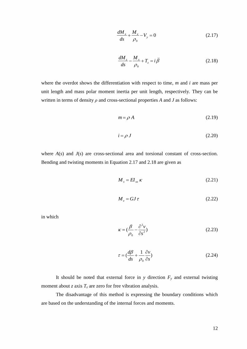
where the overdot shows the differentiation with respect to time, m and i are mass per

unit length and mass polar moment inertia per unit length, respectively. They can be

written in terms of density ρ and cross-sectional properties A and J as follows:

Am (2.19)

Ji (2.20)

where A(s) and J(s) are cross-sectional area and torsional constant of cross-section.

Bending and twisting moments in Equation 2.17 and 2.18 are given as

xxx EIM (2.21)

GJM z (2.22)

in which

)(2

2

0 s

v

(2.23)

)1

(0 s

v

ds

d

(2.24)

It should be noted that external force in y direction Fy and external twisting

moment about z axis Tz are zero for free vibration analysis.

The disadvantage of this method is expressing the boundary conditions which

are based on the understanding of the internal forces and moments.

13

2.4.2. Hamilton’s Method

The Hamilton's principle is the most powerful variational principle of

mechanics. It permits the formulation of problems of dynamics in terms of two scalar

functions, the kinetic energy and the potential energy, Moreover, it gives associated

boundary conditions where Newtonian method encounters difficulties, especially in

distributed-parameter systems.

The principle can be stated as follows; “Of all possible time histories of

displacement states that satisfy the compatibility equations and the constraints or the

kinematic boundary conditions and that also satisfy the conditions at initial and final

times t1 and t2, the history to the actual solution makes the Langrangian a minimum”

(Meirovitch 1967). The principle can be defined mathematically as follows:

0)(2

1

dtVT

t

t

(2.25)

Where T is the kinetic energy and V is the elastic strain energy due to the out of

plane motions of the curved beam. Kinetic energy and elastic strain energy of the

curved beam are given as follows;

dsivmTLS

)(2

1 2

0

2 (2.26)

dsMMV z

S

x

L

)(2

1

0 (2.27)

If Equations 2.19 and 2.20 are substituted into Equation 2.26, and Equations

2.21 and 2.22 are substituted into Equation 2.27, the following equations are written:

dsJvATLS

)(2

1 2

0

2 (2.28)

dsGJEIVLS

xx )(2

1 2

0

2 (2.29)

14

Using the kinetic and elastic energies given in Equations 2.28 and 2.29 along

with Equations 2.23 and 2.24 in Equation 2.25, governing differential equations for

vibrations of curved beams having variable radius of curvature and cross-section and

associated boundary conditions can be obtained as follows:

vAs

v

s

JG

ss

vIE

sx

00

2

2

0

2

2 1 (2.30)

J

s

v

sJG

ss

vIE x

00

2

2

0

1 (2.31)

The associated boundary conditions are:

000

2

2

0

LSx v

s

vIE

(2.32)

01

00

LS

s

v

sJG

(2.33)

01

000

2

2

0

LS

x vs

v

s

JG

s

vIE

s

(2.34)

In Equation 2.32, prime represents the differentiation with respect to s.

Physical interpretations for boundary conditions corresponding to Equations

2.32-2.34 are as follows, respectively:

a) Either bending moment is zero (pinned or free), or slope is zero (clamped).

b) Either twisting moment is zero (pinned or free), or rotation is zero (clamped).

c) Either shear force is zero (free), or displacement is zero (pinned or clamped)

If the boundary conditions of the curved beam are homogeneous as in Equations 2.32-

2.34, the solutions of Equations 2.30-2.31 are assumed as

15

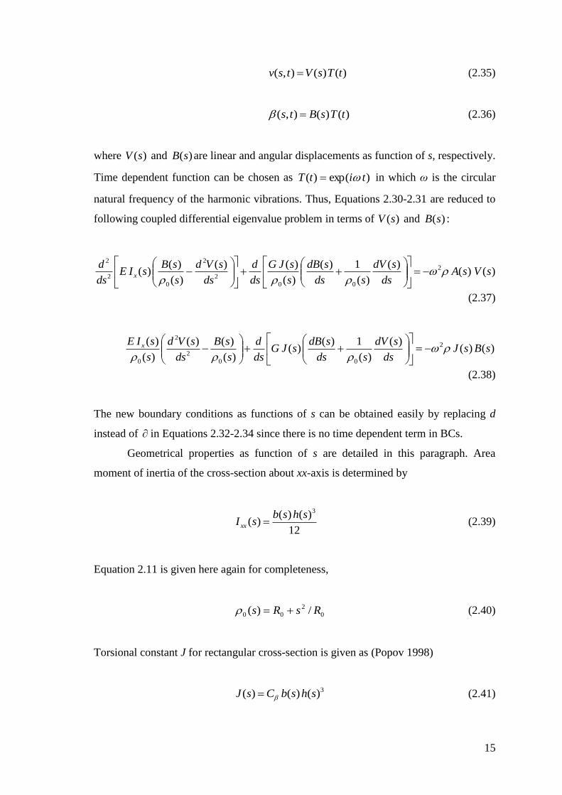
)()(),( tTsVtsv (2.35)

)()(),( tTsBts (2.36)

where )(sV and )(sB are linear and angular displacements as function of s, respectively.

Time dependent function can be chosen as )exp()( titT in which ω is the circular

natural frequency of the harmonic vibrations. Thus, Equations 2.30-2.31 are reduced to

following coupled differential eigenvalue problem in terms of )(sV and )(sB :

)()()(

)(

1)(

)(

)()(

)(

)()( 2

00

2

2

0

2

2

sVsAds

sdV

sds

sdB

s

sJG

ds

d

ds

sVd

s

sBsIE

ds

dx

(2.37)

)()()(

)(

1)()(

)(

)()(

)(

)( 2

00

2

2

0

sBsJds

sdV

sds

sdBsJG

ds

d

s

sB

ds

sVd

s

sIE x

(2.38)

The new boundary conditions as functions of s can be obtained easily by replacing d

instead of in Equations 2.32-2.34 since there is no time dependent term in BCs.

Geometrical properties as function of s are detailed in this paragraph. Area

moment of inertia of the cross-section about xx-axis is determined by

12

)()()(

3shsbsI xx (2.39)

Equation 2.11 is given here again for completeness,

0

2

00 /)( RsRs (2.40)

Torsional constant J for rectangular cross-section is given as (Popov 1998)

3)()()( shsbCsJ (2.41)

16

where the values of parameter Cβ depends on the ratio of b/h. By using the Equations

2.39-2.41 in Equations 2.37-2.38, the present problem equations are obtained to solve

by Finite Difference Method which will be explained in next section.

2.5. Natural Frequencies by Finite Difference Method

The Finite Difference Method is a numerical method for solution of differential

equations by using approximate derivatives (Hildebrand 1987).

Since the differential equations having variable coefficients are analytically

unsolvable except for equations having special combinations of coefficients, the Finite

Difference Method can be used.

Figure 2.4. A domain divided into six subdomains for approximation

In the Finite Difference Method, the derivatives of dependent variables in the

differential equations are replaced by the finite difference approximations at mesh

points and these equations are enforced at each mesh points. Therefore, n simultaneous

algebraic equations are obtained. In this study, central difference approximation which

is detailed in Table 2.1 is used.

Therefore, differential eigenvalue problem given by Equation 2.37-2.38 and

associated boundary conditions is reduced to discrete eigenvalue problem which can be

written as follows:

XBXA ][ (2.42)

Solutions of the generalized eigenvalue problem given by Equation 2.42 can be

obtained by a mathematical software such as Matlab, Mathematica or Maple.

0 1 2 3 4 5 6

0 VI V IV III II I

17

Table 2.1. Finite difference equations

Term Central Difference Expressions for required derivatives of V(s) and B(s)

ds

dV

h

iViV

2

)1()1(

2

2

ds

Vd 2

)1()(2)1(

h

iViViV

3

3

ds

Vd 32

)2()1(2)1(2)2(

h

iViViViV

4

4

ds

Vd 4

)2()1(4)(6)1(4)2(

h

iViViViViV

ds

dB

h

iBiB

2

)1()1(

2

2

ds

Bd 2

)1()(2)1(

h

iBiBiB

18

CHAPTER 3

NUMERICAL RESULTS AND DISCUSSION

3.1. Introduction

In this chapter, numerical applications are carried out for curved beams with

different curvature and cross-sectional properties. The main numerical data are as

follows: bo=ho=0.01 m, E=200 GPa, G=80 GPa, ρ=7850 kg/m3, sL=0.12 m. Other data

are given in table and figure legends. The numerical results are found and compared

with FEM results obtained from solid model created in ANSYS. The results given in

tabular and graphical forms are discussed.

3.2. Comparisons and Applications for Variable Curvature and

Constant Cross-Section

In this section, as first step, in order to determine the proper number of node in

finite difference mesh, the first natural frequencies are found for different number of

node and shown in Figure 3.1.

Figure 3.1. Convergence of first natural frequency for R0=50 mm and b1=h1=0.

556.06

556.08

556.10

556.12

556.14

556.16

556.18

556.20

556.22

556.24

0 20 40 60 80 100 120 140 160n

f1 (Hz)

19

Considering the tendancy of the curve shown in Figure 3.1, the proper number of

node for FDM is selected as 100 for all calculations.

To evaluate the results of FDM for the case of variable curvature and constant

cross-section, four different solid models depending on R0 are created in ANSYS by

using 4x4x50 Solid 95 elements.

The natural frequencies found for different R0 by Finite Difference Models and

Finite Element Models are tabulated in Table 3.1 and plotted in Figure 3.2. The mode

shapes are given in Figure 3.3.

Table 3.1. Comparison of natural frequencies found for different R0 by FDM with

FEM results (b1=h1=0)

R0=50 mm R0=100 mm R0=150 mm R0=200 mm

f1 (Hz)

bending 1

FDM 556.2 562.9 564.7 565.4

FEM 569.7 568.4 566.6 565.6

f2 (Hz)

bending 2

FDM 3084.5 3157.9 3275.8 3358.3

FEM 3035.6 3115.0 3221.0 3291.0

f3 (Hz)

torsion 1

FDM 7802.6 7481.7 7186.7 7009.3

FEM 7812.2 7489.7 7244.8 7106.6

f4 (Hz)

bending 3

FDM 9556.1 9810.8 9891.1 9913.9

FEM 8968.7 9215.7 9274.6 9283.7

f5 (Hz)

bending 4

FDM 18942.1 19160.5 19227.6 19274.6

FEM 16909.0 17081.9 17155.1 17194.7

f6 (Hz)

torsion 2

FDM 21118.5 20546.6 20329.9 20217.0

FEM 21482.7 20993.2 20787.6 20689.9

f7 (Hz)

bending 5

FDM 31422.2 31798.7 31920.0 31982.1

FEM 26565.2 26778.3 26862.5 26902.5

f8 (Hz)

torsion 3

FDM 34216.9 33656.5 33486.2 33403.8

FEM 34929.3 34525.7 34379.8 34313.2

20

a) Bending 1 b) Bending 2

c) Torsion 1 d) Bending 3

e) Bending 4 f) Torsion 2

g) Bending 5 h) Torsion 3

Figure 3.2. Comparisons of natural frequencies found for different R0 by FDM with

FEM results.

550

560

570

580

50 100 150 200

Ro (mm)

f (Hz)

FEM

FDM

3000

3100

3200

3300

3400

50 100 150 200

Ro (mm)

f (Hz)

FEM

FDM

7000

7200

7400

7600

7800

50 100 150 200

Ro (mm)

f (Hz)

FEM

FDM

8900

9100

9300

9500

9700

9900

50 100 150 200

Ro (mm)

f (Hz)

FEM

FDM

16000

17000

18000

19000

20000

50 100 150 200

Ro (mm)

f (Hz)

FEM

FDM

20000

20400

20800

21200

21600

50 100 150 200

Ro (mm)

f (Hz)

FEM

FDM

26000

28000

30000

32000

50 100 150 200

Ro (mm)

f (Hz)

FEM

FDM

33000

34000

35000

50 100 150 200

Ro (mm)

f (Hz)

FEM

FDM

21

a) First bending mode

b) Second bending mode

c) First torsion mode

d) Third bending mode

Figure 3.3. Mode shapes for for R0=50 mm and b1=h1=0 (cont. on next page)

22

e) Fourth bending mode

f) Second torsion mode

g) Fifth bending mode

h) Third torsion mode

Figure 3.3. (cont.)

23

Natural frequencies are plotted in Figures 3.2.a-h separately in the order of mode

shapes to see the difference of FDM and FEM results clearly.

In order to show the effect of the R0 on the natural frequencies of the beam,

Figures 3.2.a-h are illustrated as natural ferqunecies versus R0. It can be seen from the

Figures 3.2.a-h that the results of FDM and FEM have the same tendancy except first

bending mode. For the first bending mode, the parameter R0 is very effective on the

results of FDM and FEM. It is very interesting that the FDM and FEM results are

almost the same for R0=200 mm. For other cases, it is obvious that when the mode

number increases, the differences become more significant.

The beam is in x-z plane as shown in Figures 2.1 or 2.3. The mode shapes given

in Figure 3.3.a-h are obtained from FEM. In these figures, bending displacements are in

y direction and torsional displacements are about local z axis.

3.3. Applications for Variable Curvature and Cross-Section

Numerical applications for the case of variable curvature and variable cross-

section are presented for various radius of curvatures in this section.

Effects of parameter R0 on natural frequencies for different tapering ratios are

studied and the results are given in Table 3.2-4.

Table 3.2. Effects of parameter R0 on natural frequencies for b1=h1=2/120

R0=50 mm R0=100 mm R0=150 mm R0=200 mm

f1 (Hz) 610.87 617.486 619.338 619.993

f2 (Hz) 3059.72 3113.66 3201.41 3260.86

f3 (Hz) 8749.87 8428.42 8229.44 8117.2

f4 (Hz) 8985.88 9218.79 9215.24 9188.5

f5 (Hz) 17232.7 17436.8 17517.9 17561.1

f6 (Hz) 21528.1 20964.9 20733.5 20623.2

f7 (Hz) 28486.4 28772.1 28878.8 28929.5

f8 (Hz) 34413.5 33915.4 33745.5 33667.3

24


R0=50 mm R0=100 mm R0=150 mm R0=200 mm

f1 (Hz) 685.64 692.20 694.00 694.63

f2 (Hz) 3005.03 3041.14 3102.00 3142.39

f3 (Hz) 7979.17 8060.64 8111.62 8148.87

f4 (Hz) 10580.03 10378.29 10132.53 9968.70

f5 (Hz) 15430.34 15592.03 15659.79 15693.52

f6 (Hz) 22246.65 21760.07 21551.76 21454.86

f7 (Hz) 25384.20 25560.93 25638.50 25674.15

f8 (Hz) 34764.11 34399.54 34255.01 34188.85


R0=50 mm R0=100 mm R0=150 mm R0=200 mm

f1 (Hz) 797.00 803.45 805.16 805.72

f2 (Hz) 2930.13 2951.87 2990.30 3015.51

f3 (Hz) 7133.35 7217.49 7267.87 7296.38

f4 (Hz) 12720.34 12602.01 12392.65 12259.42

f5 (Hz) 13710.32 13671.04 13680.67 13690.12

f6 (Hz) 21633.21 21871.94 21967.59 22022.12

f7 (Hz) 24084.31 23533.63 23312.78 23198.85

f8 (Hz) 32110.80 32415.48 32528.06 32583.23

By using the numerical results given in Tables 3.2-4, different types of figures

can be plotted. The first group plots are given in Figures 3.4-6 separately in the order of

mode shapes, to see the effect of R0 on the natural frequencies for three different values

of taper parameters b1=h1 in the range of each natural frequency. The second group

plots are given in Figure 3.7 to combine all the parameters in one plot.

25

a) Natural frequency 1 b) Natural frequency 2

c) Natural frequency 3 d) Natural frequency 4

e) Natural frequency 5 f) Natural frequency 6

g) Natural frequency 7 h) Natural frequency 8

Figure 3.4. Natural frequencies for b1=h1=2/120.

610

612

614

616

618

620

622

50 100 150 200

Ro (mm)

f (Hz)

3000

3050

3100

3150

3200

3250

3300

50 100 150 200

Ro (mm)

f (Hz)

8000

8100

8200

8300

8400

8500

8600

8700

8800

50 100 150 200

Ro (mm)

f (Hz)

8950

9000

9050

9100

9150

9200

9250

50 100 150 200

Ro (mm)

f (Hz)

17200

17300

17400

17500

17600

50 100 150 200

Ro (mm)

f (Hz)

20400

20600

20800

21000

21200

21400

21600

50 100 150 200

Ro (mm)

f (Hz)

28400

28500

28600

28700

28800

28900

29000

50 100 150 200

Ro (mm)

f (Hz)

33600

33800

34000

34200

34400

34600

50 100 150 200

Ro (mm)

f (Hz)

26






684

686

688

690

692

694

696

50 100 150 200

Ro (mm)

f (Hz)

2950

3000

3050

3100

3150

50 100 150 200

Ro (mm)

f (Hz)

7950

8000

8050

8100

8150

8200

50 100 150 200

Ro (mm)

f (Hz)

9900

10000

10100

10200

10300

10400

10500

10600

10700

50 100 150 200

Ro (mm)

f (Hz)

15400

15450

15500

15550

15600

15650

15700

15750

50 100 150 200

Ro (mm)

f (Hz)

21400

21600

21800

22000

22200

22400

50 100 150 200

Ro (mm)

f (Hz)

25350

25400

25450

25500

25550

25600

25650

25700

50 100 150 200

Ro (mm)

f (Hz)

34100

34200

34300

34400

34500

34600

34700

34800

50 100 150 200

Ro (mm)

f (Hz)

27






796

798

800

802

804

806

808

50 100 150 200

Ro (mm)

f (Hz)

2920

2940

2960

2980

3000

3020

50 100 150 200

Ro (mm)

f (Hz)

7100

7150

7200

7250

7300

7350

50 100 150 200

Ro (mm)

f (Hz)

12200

12300

12400

12500

12600

12700

12800

50 100 150 200

Ro (mm)

f (Hz)

13660

13670

13680

13690

13700

13710

13720

50 100 150 200

Ro (mm)

f (Hz)

21600

21700

21800

21900

22000

22100

50 100 150 200

Ro (mm)

f (Hz)

23000

23200

23400

23600

23800

24000

24200

50 100 150 200

Ro (mm)

f (Hz)

32000

32100

32200

32300

32400

32500

32600

32700

50 100 150 200

Ro (mm)

f (Hz)

28

a) First natural frequencies

b) Second natural frequencies

c) Third natural frequencies

Figure 3.7. Natural frequencies for different b1=h1 (cont. on next page)

500

550

600

650

700

750

800

850

50 100 150 200

Ro (mm)

f1 (Hz)

b1=h1=0 b1=h1=2/120

b1=h1=4/120 b1=h1=6/120

2900

3000

3100

3200

3300

3400

50 100 150 200

Ro (mm)

f2 (Hz)

b1=h1=0 b1=h1=2/120

b1=h1=4/120 b1=h1=6/120

6500

7000

7500

8000

8500

9000

50 100 150 200

Ro (mm)

f3 (Hz)

b1=h1=0 b1=h1=2/120

b1=h1=4/120 b1=h1=6/120

29

d) Fourth natural frequencies

e) Fifth natural frequencies

f) Sixth natural frequencies

Figure 3.7 (cont.)

6500

7500

8500

9500

10500

11500

12500

13500

50 100 150 200

Ro (mm)

f4 (Hz)

b1=h1=0 b1=h1=2/120

b1=h1=4/120 b1=h1=6/120

12000

13000

14000

15000

16000

17000

18000

19000

20000

50 100 150 200

Ro (mm)

f5 (Hz)

b1=h1=0 b1=h1=2/120

b1=h1=4/120 b1=h1=6/120

20000

20500

21000

21500

22000

22500

50 100 150 200

Ro (mm)

f6 (Hz)

b1=h1=0 b1=h1=2/120

b1=h1=4/120 b1=h1=6/120

30

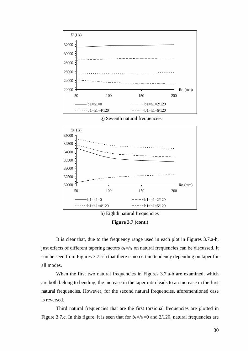
g) Seventh natural frequencies

h) Eighth natural frequencies

Figure 3.7 (cont.)

It is clear that, due to the frequency range used in each plot in Figures 3.7.a-h,

just effects of different tapering factors b1=h1 on natural frequencies can be discussed. It

can be seen from Figures 3.7.a-h that there is no certain tendency depending on taper for

all modes.

When the first two natural frequencies in Figures 3.7.a-b are examined, which

are both belong to bending, the increase in the taper ratio leads to an increase in the first

natural frequencies. However, for the second natural frequencies, aforementioned case

is reversed.

Third natural frequencies that are the first torsional frequencies are plotted in

Figure 3.7.c. In this figure, it is seen that for b1=h1=0 and 2/120, natural frequencies are

22000

24000

26000

28000

30000

32000

50 100 150 200

Ro (mm)

f7 (Hz)

b1=h1=0 b1=h1=2/120

b1=h1=4/120 b1=h1=6/120

32000

32500

33000

33500

34000

34500

35000

50 100 150 200

Ro (mm)

f8 (Hz)

b1=h1=0 b1=h1=2/120

b1=h1=4/120 b1=h1=6/120

31

decreased with the increasing of R0. On the contrary, this tendancy is inverted for

b1=h1=4/120 and 6/120.

For the fourth natural frequencies, the effects similar to the third natural

frequencies are also observed. But in this time, the decrease turns into an increase. The

reason of this change is directly related to mode shapes. Third natural frequencies are

related with torsional motion whereas fourth natural frequencies are bending motions.

Taper ratios affect the fifth natural frequencies in similar fashion with the

increasing of R0.

Sixth natural frequencies that are the second torsional frequencies are plotted in

Figure 3.7.f. It is partially similar to Figure 3.7.c. The only difference is the variation of

natural frequencies with R0 for the taper parameters b1=h1=6/120. It is similar for the

curve for b1=h1=0.

Seventh natural frequencies are very similar to the second and the fifth natural

frequencies. Taper effects are the same in these three groups.

Eighth natural frequencies that are the third torsional frequencies are plotted in

Figure 3.7.h. The exceptional behavior can be seen for b1=h1=6/120.

Considering the all plots given in Figures 3.7.a-h, as the parameter R0 increases,

the effects of taper parameters become more important. It can be said that R0=100 mm

is a critical value since the tendency of some curves in these figures are changed

sharply.

32

CHAPTER 4

CONCLUSIONS

In this study, the differential equations governing the free out-of plane vibrations

of curved beams with variable curvature and variable cross-section are presented. The

equations of motions are derived by using both Newtonian Method and the Hamilton’s

principle. Since the coefficients of the derived differential equations are not constant, it

is not possible to express an exact solution.

For free vibration analysis, the coupled differential eigenvalue problem obtained

by using separation of variables technique. It is reduced to discrete eigenvalue problem

by using FDM (Finite Difference Method).

In the existing literature, for the free out-of-plane vibrations of curved beams,

most of the researchers investigated the symmetrical boundary conditions such as both

ends fixed, pinned or free conditions.

With this study, as far as the author is aware, for the first time, the natural

frequencies for out-of plane vibrations of curved beams with variable curvature and

variable cross-section as well as mode shapes are studied and presented for fixed-free

condition.

In order to validate the developed computer program to solve the differential

eigenvalue problem based on FDM, the solid models are created for Finite Element

analysis. The results, found out from FDM, are compared with the results from FEM

(Finite Element Method). Good agreement is obtained for lower modes.

The effects of taper and curvature parameters on natural frequencies are found

for the linearly tapered curved beams in the shape of catenary with selected geometries.

33

REFERENCES

Chang, T. and Volterra, E. 1969. Upper and lower bounds for frequencies of elastic

arcs. The Journal of the Acoustical Society of America 46(5): 1165-1174.

Hildebrand, Francis B. 1987. Introduction to numerical analysis. New York: Dover

Publications.

Huang, C. S., Tseng, Y. P. and Chang, S.H. 1998. Out-of-plane dynamic responses of

non-circular curved beams by numerical laplace transform. Journal of Sound

and Vibration 215: 407-424

Huang, C. S., Tseng, Y. P., Chang, S.H. and Hung, C. L. 2000. Out-of-plane dynamic

analysis of beams with arbitrarily varying curvature and cross-section by

dynamic stiffness matrix method. International Journal of Solids and

Structures 37: 495-513

Irie, T., Yamada, G. and Takahashi, I. 1980. The steady state out-of-plane response of a

Timoshenko curved beam with internal damping. Journal of Sound and

Vibration 71: 145-156

Kawakami, M., Sakiyama, T., Matsuda, H. and Morita, C. 1995. In-plane and out-of-

plane free vibrations of curved beams with variable sections. Journal of Sound

and Vibration 187: 381-401

Kim, N. I., Seo, K. J. and Kim, M. Y. 2003. Free vibration and spatial stability of non-

symmetric thin-walled curved beams with variable curvatures. International

Journal of Solids and Structures 40: 3107-3128

Lee, S. Y. and Chao, J. C. 2000. Out-of-plane vibrations of curved non-uniform beams

of constant radius. Journal of Sound and Vibration 238: 443-458

Lee, B. K., Oh, S. J., Mo, J. M. and Lee, T. E. 2008. Out-of-plane free vibrations of

curved beams with variable curvature. Journal of Sound and Vibration 318:

227-246

Love, Augustus E.H. 1944. A treatise on the mathematical theory of elasticity. New

York: Dover Publications.

Meirovitch, Leonard 1967. Analytical methods in vibrations. New York: Macmillan

Publishing Co.

Ojalvo, I.U. 1962. Coupled twist-bending vibrations of incomplete elastic rings,

International Journal of Mechanical Science 4: 53-72

Popov, E.P., Balan, T.A. 1998. Engineering Mechanics of Solids. New Jersey: Prentice

Hall.

34

Rao, Singiresu S. 2007. Vibration of continuous systems. New Jersey: John Wiley &

Sons, Inc.

Riley, K. F., Hobson, M. P. and Bence, S. J., 2006, Mathematical Methods for Physics

and Engineering, New York: Cambridge University Press.

Suzuki, K., Aida, H. and Takahashi, S. 1978. Vibrations of curved bars perpendicular to

their planes. Bulletin of the JSME 21: 1685-1695

Suzuki, K. and Takahashi, S. 1981. Out-plane vibrations of curved bars considering

shear deformation and rotator inertia. Bulletin of the JSME 24: 1206-1213

Suzuki, K., Kosawada, T. and Takahashi, S. 1983. Out-of-plane vibrations of curved

bars with varying cross-section. Bulletin of the JSME 26:268-275

Takahashi, S. and Suzuki K. 1977. Vibrations of elliptic arc bar perpendicular to its

plane. Bulletin of the JSME 20: 1409-1416

Tüfekçi, E. and Doğruer O. Y. 2006. Exact solution of out-of-plane problems of an arch

with varying curvature and cross section. Journal of Engineering Mechanics

132: 600-609

Volterra, E. and Morell, J. D. 1961. Lowest natural frequency of elastic arc for

vibrations outside of the plane of initial curvature. Journal of Applied

Mechanics 28: 624-627.

Volterra, E. and Morell, J. D. 1961. Lowest natural frequency of elastic hinged arcs. The

Journal of the Acoustical Society of America 33: 1787-1790

Wang, T. M. 1975. Fundamental frequency of clamped elliptic arcs for vibrations

outside the plane of initial curvature. Journal of Sound and Vibration 42: 515-

519

Yardimoglu, B. 2010. Dönen eğri eksenli çubukların titreĢim özelliklerinin sonlu

elemanlar yöntemi ile belirlenmesi. 2. Ulusal Tasarım Ġmalat ve Analiz

Kongresi, Balıkesir, 514-522

Yıldırım, V. 1997. In-plane and out-of-plane free vibration analysis of Archimedes-type

spiral springs. Journal of Applied Mechanics 64:557-561

Documents

OUT-OF-PLANE VIBRATIONS OF PLANAR CURVED …library.iyte.edu.tr/tezler/master/makinamuh/T001031.pdf · OUT-OF-PLANE VIBRATIONS OF PLANAR CURVED BEAMS HAVING VARIABLE CURVATURE AND