O ti i ation Method foOptimization Methods for Design of Spatial StructuresDesign of Spatial Structures

Makoto OhsakiMakoto OhsakiKyoto University, Japan

Form finding (Structural Morphology)Form finding (Structural Morphology)• Equilibrium shape of cable net, membrane, tensegrity.

i i l f ( if i ) i f• Minimal surface (= uniform tension)，Hanging surface.⇒ Optimization problem

Shape optimizationD l d i h i l d i l• Developed in mechanical eng. and aeronautical eng.

• Application of optimization methods to structural eng. i i h h f h i l i f i f• Optimize the shapes of mechanical parts, wing of aircrafts.

HeuristicsHeuristics• Genetic algorithm, Simulated annealing, etc.

Minimal surface problem

• For a given boundary, find the surface such that

Minimize total area• Simple boundary

⇒ anal tical sol tion (HP s rface)⇒ analytical solution (HP surface)• Complex boundary

⇒ numerical methods (optimization)

Minimum energy problem

• For a given boundary and force of each cable member, find the shape such that

Minimize total potential (strain) energyp ( ) gy• Uniform force

⇒ minim m length net ork⇒ minimum length network(HP surface)

• Complex boundary⇒ numerical methods (optimization)⇒ numerical methods (optimization)

What is structural optimization?

• Application of optimization methods (mathematical programming) to structural design(mathematical programming) to structural design

• Minimize cost under constraints on mechanical performanceperformance

• Define optimization problem⇒ Optimal solution⇒ Optimal solution

• Reformulate the problem or change the parameter values if the solution is not acceptablevalues if the solution is not acceptable(basically interactive)

Illustrative example

PN 21 = 22 −=N

12A

P=σ 2 A

P−=σ

11 A 2

2 A

( )AA

AAPLU y21 22+

=EAAy

21

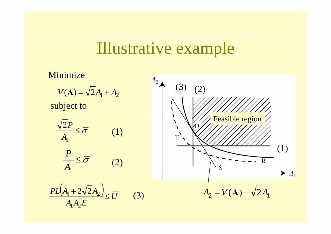
Illustrative exampleMinimize

2)( AAV A (2)(3)212)( AAV +=A

subject to

(2)( )

F ibl iσ≤

1

2A

P(1)

Feasible region

σ≤−1A

P(2)

(1)

1

( ) UAAPL≤

+ 21 22 (3) 12 2)( AVA −= A( ) UEAA

≤21

(3) 12 )(

Example of plane truss

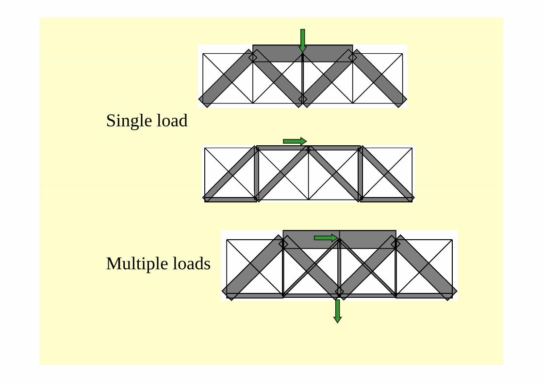
Single load

Multiple loads

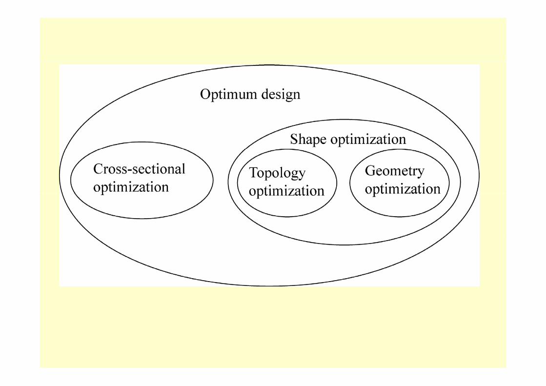
Topology optimizationp gy p

G i i iGeometry optimization

Illustrative example

Number ofdivision 2 3 4 5 6division

Totalvolume 16.20 15.33 15.30 15.60 16.07volume

Structural optimization problem

• Minimize objective functionC t i ht t– Cost, weight, etc.

• ConstraintsR (di l ) h i l– Response (displacement, stress)，mechanical performance

– Geometrical constraintsGeometrical constraints– Lower and upper bound for variables

• VariablesVariables– Cross-sectional areas, nodal coordinates, existence of

members (topology)( p gy)

Optimization problem

)(xFE

Minimize

0)( =xiG ),,1( ENi …=

0( ≤x)iH ),,1( INi …=Subject to

( )i

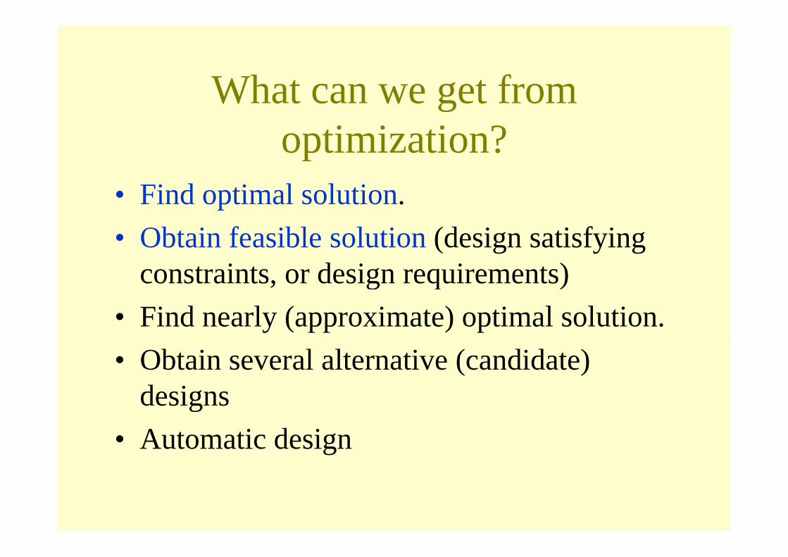
What can we get fromWhat can we get from optimization?optimization?

• Find optimal solution.• Obtain feasible solution (design satisfying

constraints or design requirements)constraints, or design requirements)• Find nearly (approximate) optimal solution.• Obtain several alternative (candidate)

designsdesigns• Automatic design

N l ti l Gl b ll ti lNearly optimal solution

Globally optimal solution

Fesible solution

Design spaceDesign space

Optimization Algorithm

• Nonlinear ProgrammingObj ti f ti d t i t ti– Objective function and constraints are continuous functions of variables.

– Gradient-based approachGradient based approach.– Optimailty criteria approach

• Integer programmingInteger programming(Combinatorial programming)– Global search and local search.– Branch-and-bound method.– Heuristics.

O ti i tiOptimization algorithm

StructuralSensitivity analysis

Structural analysis

Optimization of surface shape

Bezier surface

Round surfaceRound surface

Minimize [ ] dSrE ∫ −−= 20cx

x: point on surface: specified center of curvature0c p

r: specified radius0

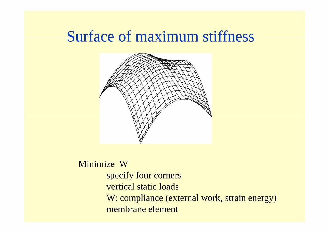
Surface of maximum stiffnessSurface of maximum stiffness

Minimize Wspecify four cornersvertical static loadsW li ( t l k t i )W: compliance (external work, strain energy)membrane element

Trade-off designTrade off design

Minimize Eesubject to W<Wopt + dW

Li fFour centers of curvature

Lines of center of curvaturecurvature

Construction process ofConstruction process of membrane structuresmembrane structures

Membrane fabric structure• Earthquake motion or buckling

does not play a key role.does o p ay a ey o e.• [Level-0]

Initial pretension forces are uniformly distributedInitial pretension forces are uniformly distributed.• [Level-1]

Nat ral freq encNatural frequency > lower bound defined by dynamic instability.

l• [Level-2] Deformation < limit defined by wrinkling and

diponding.

Performance measures of membrane

wrinkling ponding

1 Define target equilibrium surface (minmal1. Define target equilibrium surface (minmal surface)

2 C h f i h di i f d i li2. Cut the surface in the directions of geodesic lines.3. Reduce the prestress and obtain cutting patterns.

• Types of minimal surfaces are limited.E d i l li• Error due to material nonlinearty.

• Geometrically nonlinear analysis is neeeded to modify the cutting patterns to obtain the desired shape.

Developability conditions

Elements on surface Elements on plane sheetElements on surface Elements on plane sheet

Lengths of connecting edges are sameSum of the angle around a node is 360 deg.

Developability conditions

σδ A=L σδ A=Lσδ Aθ =0C =LδdθD =δ dθD =δ

σ : stress vectordD,C,B,A, : known matrices and vector

S i i i f ifi d hStress optimization for specified shapeMinimize (σ σ*)T(σ σ*)Minimize (σ-σ )T(σ-σ )subject to equilibrium equation

developability condition

Solve QP by solving linear equationsSolve QP by solving linear equationsOptimal solution is a function of shape parameters

Shape optimization using Lagrange multipliers

An HP-type membrane and the cutting pattersyp g p

O ti l h d li t i tOptimal shape under compliance constraint

Optimal shape Reverse warp and weft

• Increase curvature in the warp direction

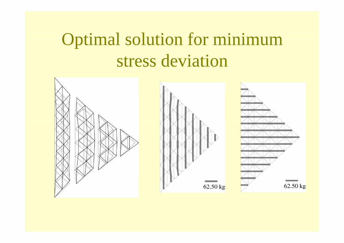
Optimal solution for minimumOptimal solution for minimum stress deviationstress deviation

Model 2

Cutting sheets

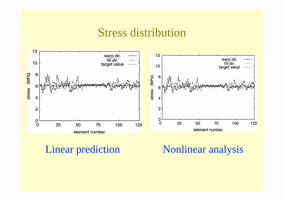
Stress distributionStress distribution

Li di i N li l iLinear prediction Nonlinear analysis

Optimum seismic design ofOptimum seismic design of trussestrusses

• Multiple components of earthquakes including vertical motionsvertical motions.

• Vertical response against horizontal motion can be criticalcritical.– No definition of magnitude.

Possibly 1/3 to 1/2 of horizontal motion– Possibly 1/3 to 1/2 of horizontal motion.• Spatial variation of earthquake motion.

Eff t f hi h d d d i t ti f• Effect of higher order modes and interaction of modes.

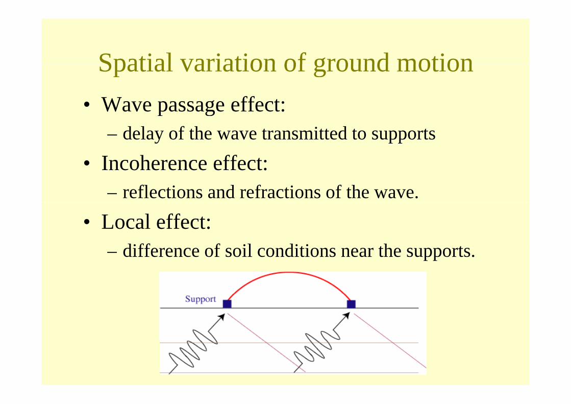
Spatial variation of ground motionSpatial variation of ground motion• Wave passage effect:Wave passage effect:

– delay of the wave transmitted to supports I h ff• Incoherence effect:– reflections and refractions of the wave.

• Local effect:diff f il diti th t– difference of soil conditions near the supports.

Coherence functionCoherence functionγij(iω) = exp[-(αωdij/vs)2]exp[i(βωdLij/vapp)]γ (iω) exp[ (αωd /vs) ]exp[i(βωd /vapp)]

i h f tα: incoherency factordij: horizontal distance between SDOFsdLij: projected distance of dij to

horizontal planepvs: velocity of shear wavevapp: apparent velocity of shear wavevapp: apparent velocity of shear waveβ: 0 or 1

Algorithm

1. Define parameters of soil condition and seismic1. Define parameters of soil condition and seismic motion.

2. Assign geometry and material of the structure.2. Assign geometry and material of the structure.3. Initialize A and optimize the structure as:

a Analysis:a. Analysis:I. Eigenvalue analysis.II Compute coherency function power spectrum etcII. Compute coherency function, power spectrum, etc.

b. Design sensitivity analysisc. Modify A and go to 3-(a) if not converged.y g ( ) g

4. Carry out post-optimal analysis.

An arch-type frame

Without spatial variation (V=1.63454)

With spatial variation (V=1.71497)

Buckling optimization of singleBuckling optimization of single-layer latticed shellslayer latticed shells

• Define performance based onb kli d t ti l dbuckling under static loads:

• Nonlinear buckling g> lower bound

Li b kli / k kd f• Linear buckling / knockdown factor > lower bound

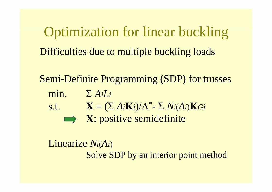
Optimization for linear bucklingOptimization for linear bucklingDifficulties due to multiple buckling loadsDifficulties due to multiple buckling loads

Semi-Definite Programming (SDP) for trussesmin Σ AiLimin. Σ AiLis.t. X = (Σ AiKi)/Λ*- Σ Ni(Ai)KGi

X: positive semidefiniteX: positive semidefinite

i iLinearize Ni(Ai)Solve SDP by an interior point method

Optimum design (nonlinear buckling)

Minimize V(A)subject to Λj > Λ*, (j=1,2,…,s)

λj>0 (j=s+1 s+2 q)λj>0, (j=s+1,s+2,…,q)

Limit pointLimit point

(hill-top branching)

Bifurcation path

A 132-bal spherical truss

Optimum cross-sectional areas

Concentrated load Distributed loads

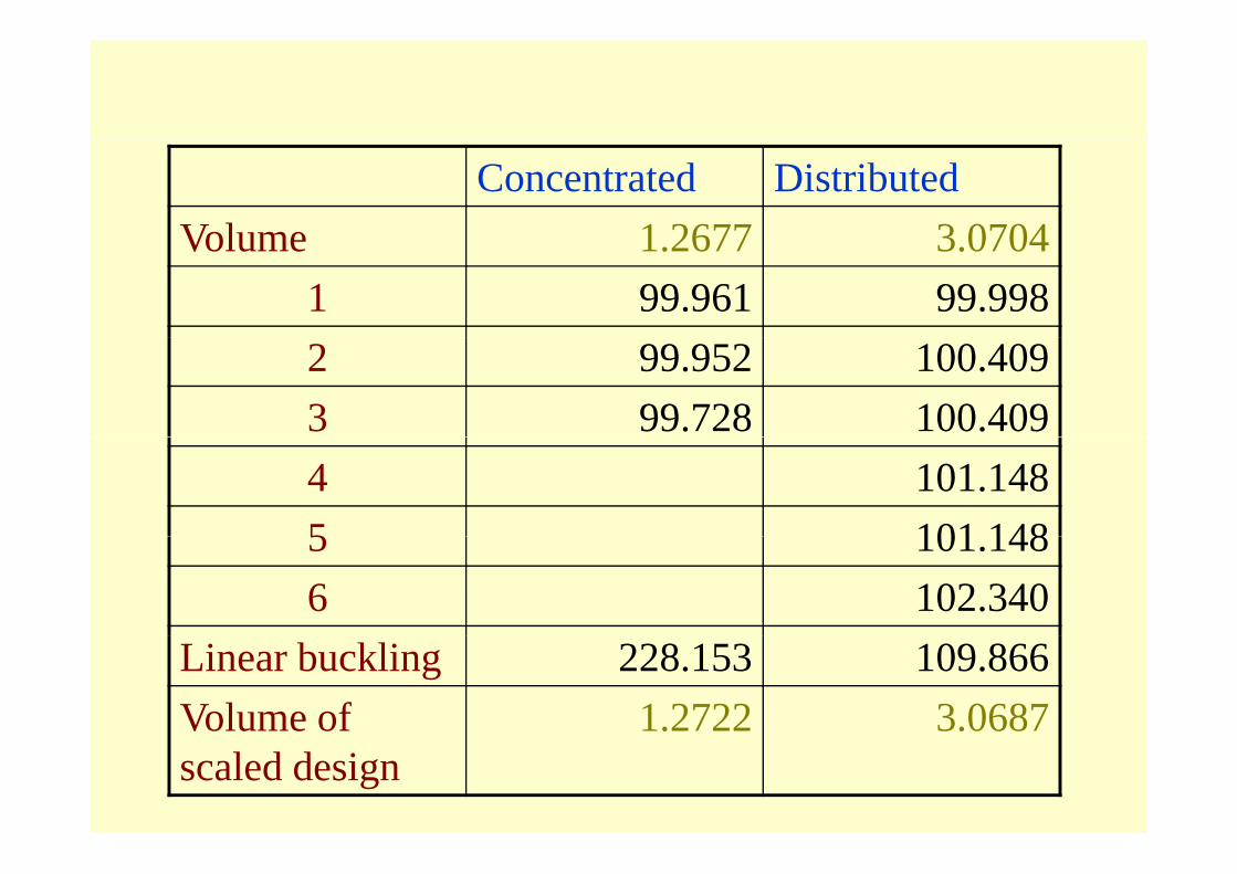
Concentrated DistributedVolume 1 2677 3 0704Volume 1.2677 3.0704

1 99.961 99.9982 99.952 100.4093 99.728 100.4094 101.1485 101 1485 101.1486 102.340

Linear buckling 228.153 109.866Volume of 1.2722 3.0687scaled design

Heuristic methods for usingHeuristic methods for using standard sectionsstandard sections

• Select cross-sections from list or catalog of standard sections.

• Integer programming problem orInteger programming problem or combinatorial optimization problem.

i h d d b h d b d• Enumeration method and branch-and-bound method for global optimization.

• Heuristics for approximate optimization.

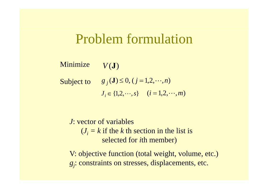
Problem formulation

)(JVMinimize

),,2,1(,0)( njg j =≤J

}21{ sJi ∈ ),,2,1( mi =

Subject to},,2,1{ sJi ∈ ),,2,1( mi

J: vector of variables(Ji = k if the k th section in the list is

l d f h b )selected for ith member)

V: objective function (total weight, volume, etc.)gj: constraints on stresses, displacements, etc.

Basic algorithm of heuristics

• [Step 1] Assign initial solution.• [Step 2] Generate neighborhood solutions,

and select a solution based on a local searchand select a solution based on a local search algorithm.

d h l i i d• [Step 3] Update the solution in accordance with the algorithm.

• [Step 4] Go to Step 2 if not converged.

Greedy method

• [Step 1] Assign an initial solution that does not satisfy the constraints; e g choose the smallestsatisfy the constraints; e.g. choose the smallest value for all variables for the case where the constraint functions gj(J) are decreasing functionsconstraint functions gj(J) are decreasing functions of J.

• [Step 2] Move to a neighborhood solution which[Step 2] Move to a neighborhood solution which most efficiently improves the objective function and constraints.

• [Step 3] Go to Step 2 if one of the constraints is not satisfied.

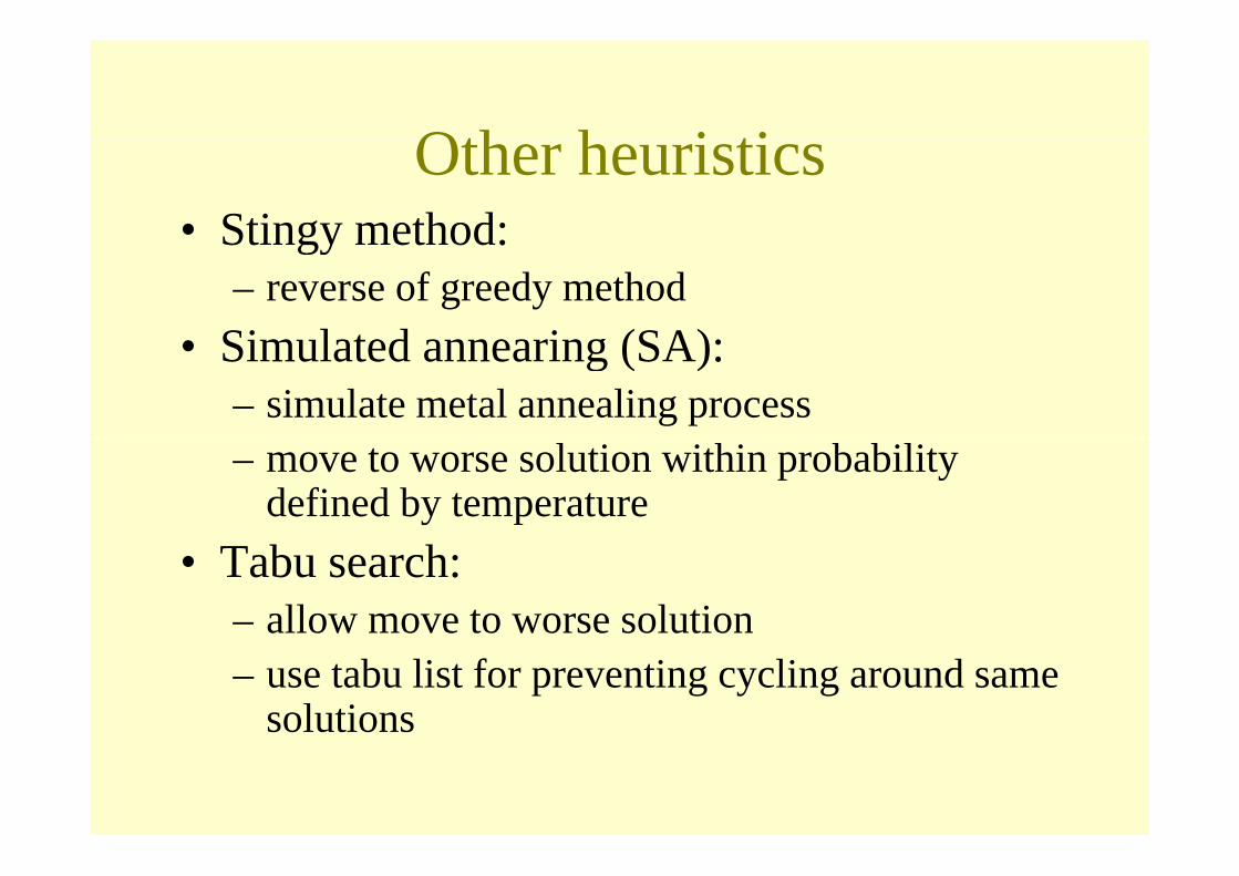
Oth h i tiOther heuristics• Stingy method:Stingy method:

– reverse of greedy methodSi l t d i (SA)• Simulated annearing (SA):– simulate metal annealing process– move to worse solution within probability

defined by temperature• Tabu search:

– allow move to worse solution– use tabu list for preventing cycling around same

solutions

Example of single layer spatialExample of single-layer spatial frameframe

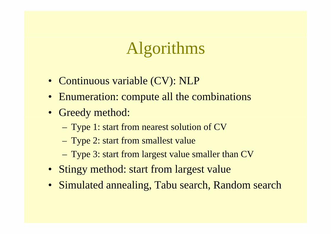
Algorithms

• Continuous variable (CV): NLP• Enumeration: compute all the combinations• Greedy method:y

– Type 1: start from nearest solution of CV– Type 2: start from smallest valueype : s a o s a es va ue– Type 3: start from largest value smaller than CV

• Stingy method: start from largest value• Stingy method: start from largest value• Simulated annealing, Tabu search, Random search

Optimization result (1)

Continuous Greedy h d

Enumera-i (

Greedy h d StingyContinuous

variable method (type 1)

tion (exact solution)

method (type 2)

Stingy method

V 2.504 3.831 3.766 3.996 4.005

Max. stress ratio 1.000 0.9957 0.9746 0.9409 0.8961

Number of analysis 1233 1237 489331 16 14

Optimization result (2)

Simulated Random Tabu LS around i

Greedy h dSimulated

annealingRandom search

Tabu search continuous

solutionmethod (type 3)

V 3.831 3.766 3.870 3.766 4.157

Max. stress ratio 0.9980 0.9746 0.8961 0.8441 0.9746

Number of analysis 2000 2000 100 2256 1244

Performances of heuristics

• The exact solution or a good approximate l ti b f d b SA dsolution can be found by SA or random

search.• Sometimes a solution with large objective

value may be found by greedy method or y y g ystingy method.

• The optimal solution mey not exist near theThe optimal solution mey not exist near the solution with continuous variables.

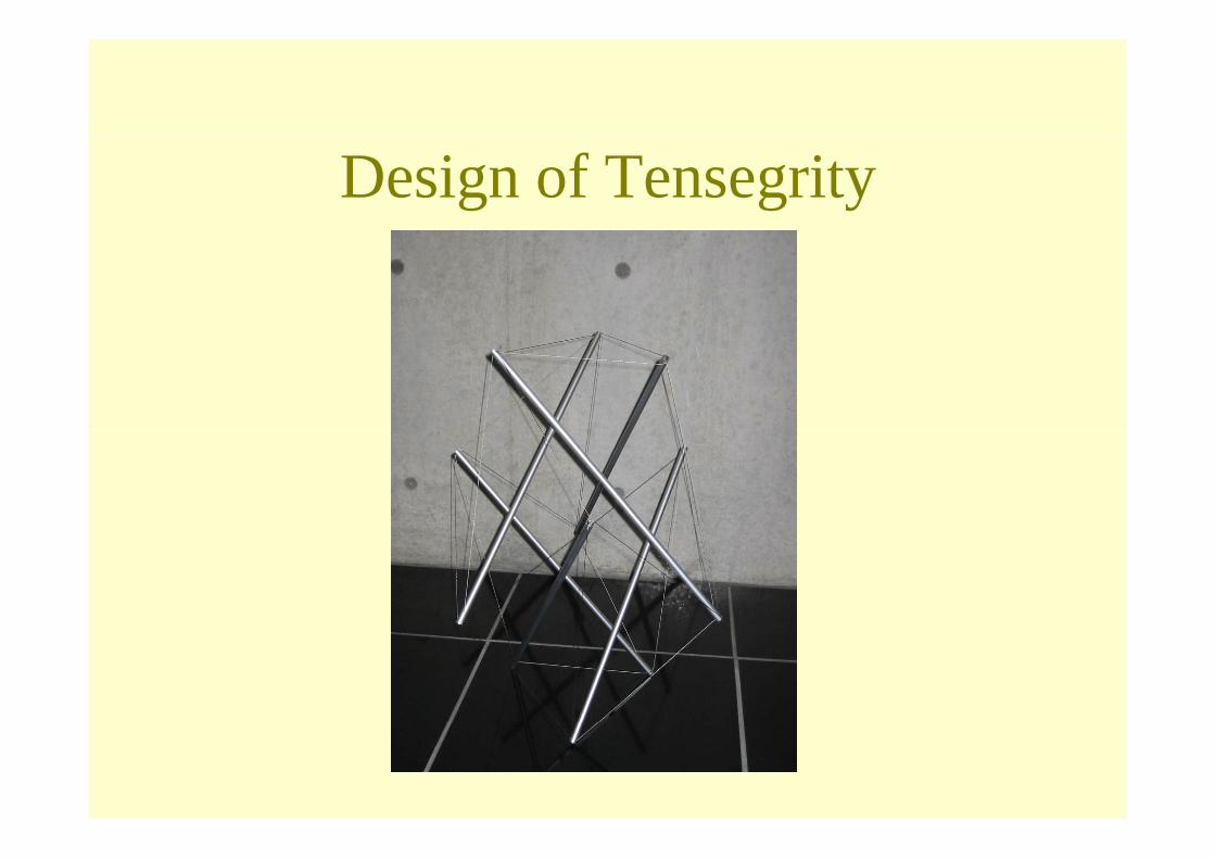
Design of Tensegrity

Stiffness by prestressWithout prestress Prestresses state

Unstable St blUnstable Stable

Form-finding process

• Equilibrium equations (self-equilibrium)DN = 0

D: equilibrium matrixqN: vector of member forces

• X: nodal coordinates• X: nodal coordinates• D depends on X• Solve D(X)N = 0 for N and X

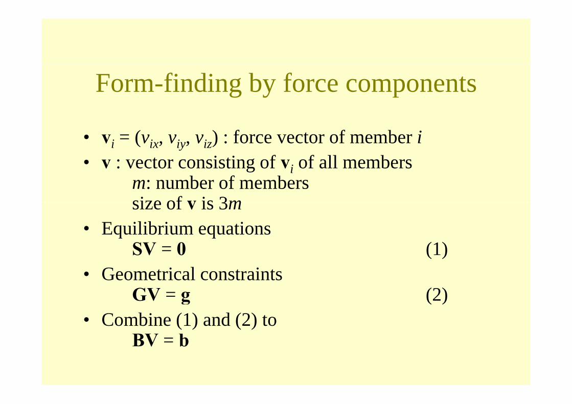
Form-finding by force components

• vi = (vix, viy, viz) : force vector of member ii i f f ll b• v : vector consisting of vi of all members

m: number of memberssize of v is 3msize of v is 3m

• Equilibrium equationsSV = 0 (1)SV = 0 (1)

• Geometrical constraintsGV = g (2)GV = g (2)

• Combine (1) and (2) toBV = bBV = b

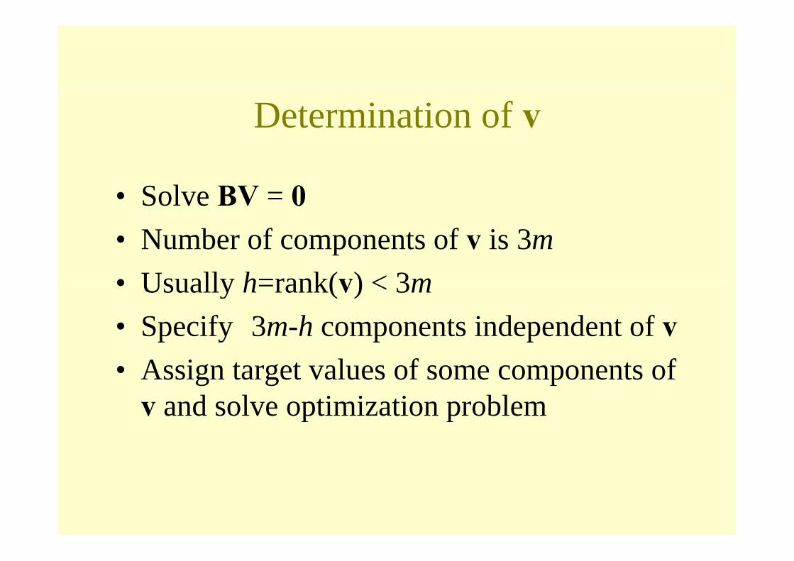
Determination of v

• Solve BV = 0• Number of components of v is 3m• Usually h=rank(v) < 3m• Usually h=rank(v) < 3m• Specify 3m-h components independent of v• Assign target values of some components of

v and solve optimization problemv and solve optimization problem

Optimization for determination of v

• Objective function

( ) ( )vvWvvv −−= T

21)(E

: target valuesW : weight coefficients

vW : weight coefficients

• Optimization problemminimize subject to

)(vEbBv =j

Example of 2D-tensegrity1111 2

92

92

52

5

111

)0(21))3((

21)1(

21)5.0(

21)( yxyx vvvvE −+−−+−+−=v

272

231

231

111

)(21)(

21))((

21 xxyxxx vvvvvv −+−+−−+

286

286

272 )(

21))((

21)(

21 yyxxyy vvvvvv −+−−+−+

Various shapes of 3D-tensegrityV ous s pes o 3 e seg y

plan elevation bird view