1

Orthogonal Neighborhood Preserving Projections: Aprojection-based dimensionality reduction technique

Effrosyni Kokiopoulou, Student member, IEEE, and Yousef Saad.

Abstract— This paper considers the problem of dimensionalityreduction by orthogonal projection techniques. The main featureof the proposed techniques is that they attempt to preserve boththe intrinsic neighborhood geometry of the data samples andthe global geometry. In particular we propose a method, namedOrthogonal Neighborhood Preserving Projections, which worksby first building an “affinity” graph for the data, in a way thatis similar to the method of Locally Linear Embedding (LLE).However, in contrast with the standard LLE where the mappingbetween the input and the reduced spaces is implicit, ONPPemploys an explicit linear mapping between the two. As a result,handling new data samples becomes straightforward, as thisamounts to a simple linear transformation. We show how to definekernel variants of ONPP, as well as how to apply the methodin a supervised setting. Numerical experiments are reported toillustrate the performance of ONPP and to compare it with afew competing methods.

Index Terms— Linear Dimensionality Reduction, Face Recog-nition, Data Visualization.

I. INTRODUCTION

The problem of dimensionality reduction appears in manyfields including data mining, machine learning and computervision, to name just a few. It is often a necessary preprocessingstep in many systems, usually employed for simplificationof the data and noise reduction. The goal of dimensionalityreduction is to map the high dimensional samples to a lowerdimensional space such that certain properties are preserved.Usually, the property that is preserved is quantified by anobjective function and the dimensionality reduction problem isformulated as an optimization problem. For instance, PrincipalComponents Analysis (PCA) is a traditional linear techniquewhich aims at preserving the global variance and relies onthe solution of an eigenvalue problem involving the samplecovariance matrix. Locally Linear Embedding (LLE) [1], [2]is a nonlinear dimensionality reduction technique which aimsat preserving the local geometries at each neighborhood.

While PCA is good at preserving the global structure, it doesnot preserve the locality of the data samples. In this paper, alinear dimensionality reduction technique is advocated, whichpreserves the intrinsic geometry of the local neighborhoods.

Work supported by NSF under grant DMS 0510131 and by the MinnesotaSupercomputing Institute.

E. Kokiopoulou is with the Swiss Federal Institute of Technology,Lausanne (EPFL), Signal Processing Institute, LTS4 lab, Bat.ELD 241, Station 11; CH 1015 Lausanne; Switzerland. Email:effrosyni.kokiopoulou@epfl.ch.

Y. Saad is with the Department of Computer Science and Engineering; Uni-versity of Minnesota; Minneapolis, MN 55455. Email: saad@cs.umn.edu.

The proposed method, named Orthogonal Neighborhood Pre-serving Projections (ONPP) [3], projects the high dimensionaldata samples on a lower dimensional space by means of alinear transformation V . The dimensionality reduction matrixV is obtained by minimizing an objective function whichcaptures the discrepancy of the intrinsic neighborhood geome-tries in the reduced space. Note that the neighborhood setsare not independent. In fact, since there is a great overlapbetween the neighborhood sets of near-by data samples, it canbe deduced that the global geometric characteristics of thedata will be preserved as well. This can also be seen from thefact that the mapping is an orthogonal projection. In principle,orthogonal projections, like PCA, will be “blind” to featuresthat are orthogonal to the span of V . However, the projectorcan be carefully selected in such a way that these features areunimportant for the task at hand. By their linearity, they willalso give good representation of the global geometry. One canview this class of methods as a compromise between PCAwhich emphasizes global structure, and LLE which is basedmainly on preserving local structure.

While one is tempted to take examples from the 3-D to 2-D linear projections, this situation provides too simplistic arepresentation of the complex situations which occur in highdimensional cases. As will be shown experimentally, linearprojections can be quite effective for certain tasks such as datavisualization. We provide experimental results which supportthis claim. In particular, experiments will confirm that ONPPcan be an effective tool for data visualization purposes and thatit may be viewed as a synthesis of PCA and LLE. In addition,ONPP can provide the foundation of nonlinear techniques,such as Kernel methods [4], [5], or Isomap [6]. In particular,we provide a framework which unifies various well-knownmethods.

ONPP constructs a weighted k-nearest neighbor (k-NN)graph which models explicitly the data topology. Similarlyto LLE, the weights are built to capture the geometry ofthe neighborhood of each point. The linear projection step isdetermined by imposing the constraint that each data sample inthe reduced space is reconstructed from its neighbors by thesame weights used in the input space. However, in contrastto LLE, ONPP computes an explicit linear mapping fromthe input space to the reduced space. Note that in LLE themapping is implicit and it is not clear how to embed newdata samples (see e.g. research efforts by Bengio et al. [7]).In the case of ONPP the projection of a new data sample isstraightforward as it simply amounts to a matrix by vector

2

product.ONPP shares some properties with Locality Preserving

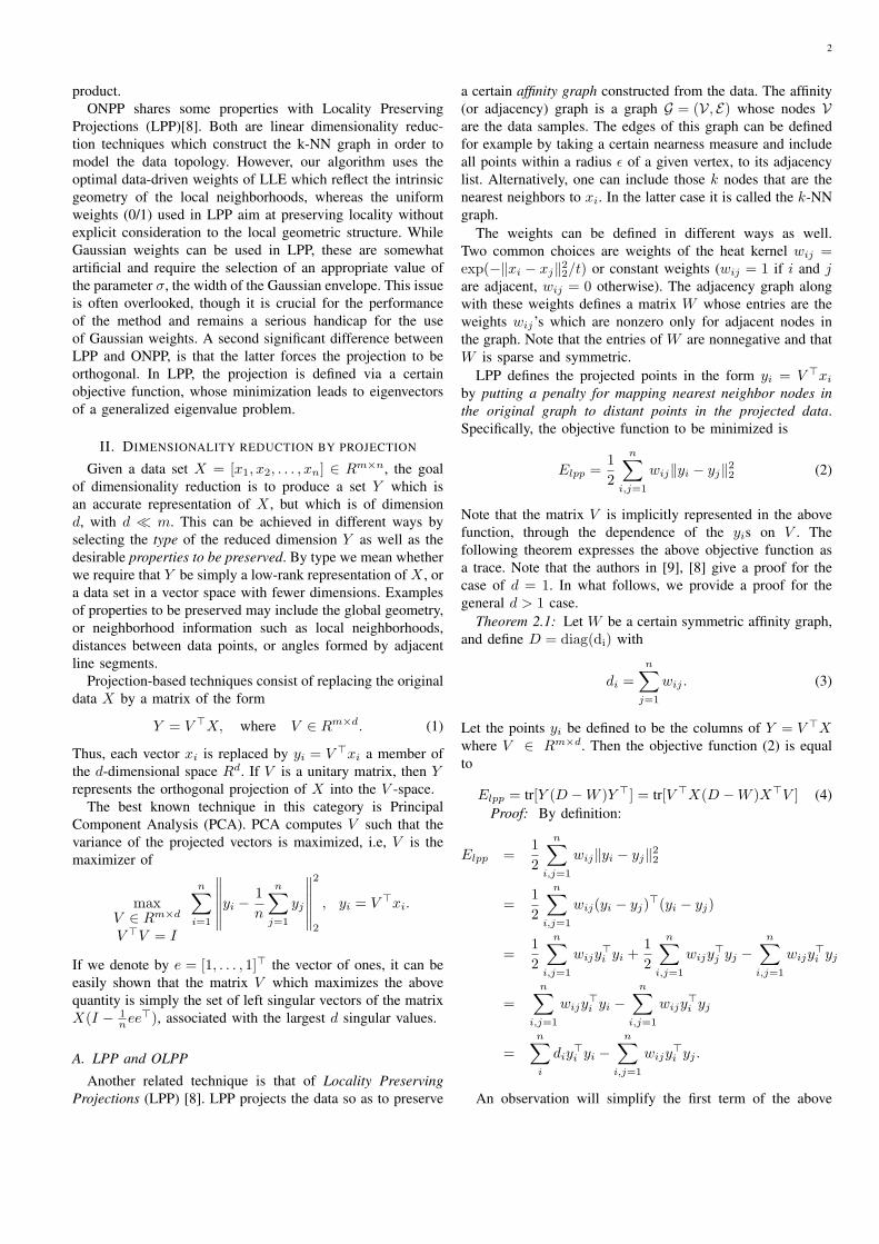
Projections (LPP)[8]. Both are linear dimensionality reduc-tion techniques which construct the k-NN graph in order tomodel the data topology. However, our algorithm uses theoptimal data-driven weights of LLE which reflect the intrinsicgeometry of the local neighborhoods, whereas the uniformweights (0/1) used in LPP aim at preserving locality withoutexplicit consideration to the local geometric structure. WhileGaussian weights can be used in LPP, these are somewhatartificial and require the selection of an appropriate value ofthe parameter σ, the width of the Gaussian envelope. This issueis often overlooked, though it is crucial for the performanceof the method and remains a serious handicap for the useof Gaussian weights. A second significant difference betweenLPP and ONPP, is that the latter forces the projection to beorthogonal. In LPP, the projection is defined via a certainobjective function, whose minimization leads to eigenvectorsof a generalized eigenvalue problem.

II. DIMENSIONALITY REDUCTION BY PROJECTION

Given a data set X = [x1, x2, . . . , xn] ∈ Rm×n, the goalof dimensionality reduction is to produce a set Y which isan accurate representation of X , but which is of dimensiond, with d ¿ m. This can be achieved in different ways byselecting the type of the reduced dimension Y as well as thedesirable properties to be preserved. By type we mean whetherwe require that Y be simply a low-rank representation of X , ora data set in a vector space with fewer dimensions. Examplesof properties to be preserved may include the global geometry,or neighborhood information such as local neighborhoods,distances between data points, or angles formed by adjacentline segments.

Projection-based techniques consist of replacing the originaldata X by a matrix of the form

Y = V >X, where V ∈ Rm×d. (1)

Thus, each vector xi is replaced by yi = V >xi a member ofthe d-dimensional space Rd. If V is a unitary matrix, then Yrepresents the orthogonal projection of X into the V -space.

The best known technique in this category is PrincipalComponent Analysis (PCA). PCA computes V such that thevariance of the projected vectors is maximized, i.e, V is themaximizer of

maxV ∈ Rm×d

V >V = I

n∑

i=1

∥∥∥∥∥∥yi − 1

n

n∑

j=1

yj

∥∥∥∥∥∥

2

2

, yi = V >xi.

If we denote by e = [1, . . . , 1]> the vector of ones, it can beeasily shown that the matrix V which maximizes the abovequantity is simply the set of left singular vectors of the matrixX(I − 1

nee>), associated with the largest d singular values.

A. LPP and OLPP

Another related technique is that of Locality PreservingProjections (LPP) [8]. LPP projects the data so as to preserve

a certain affinity graph constructed from the data. The affinity(or adjacency) graph is a graph G = (V, E) whose nodes Vare the data samples. The edges of this graph can be definedfor example by taking a certain nearness measure and includeall points within a radius ε of a given vertex, to its adjacencylist. Alternatively, one can include those k nodes that are thenearest neighbors to xi. In the latter case it is called the k-NNgraph.

The weights can be defined in different ways as well.Two common choices are weights of the heat kernel wij =exp(−‖xi − xj‖22/t) or constant weights (wij = 1 if i and jare adjacent, wij = 0 otherwise). The adjacency graph alongwith these weights defines a matrix W whose entries are theweights wij’s which are nonzero only for adjacent nodes inthe graph. Note that the entries of W are nonnegative and thatW is sparse and symmetric.

LPP defines the projected points in the form yi = V >xi

by putting a penalty for mapping nearest neighbor nodes inthe original graph to distant points in the projected data.Specifically, the objective function to be minimized is

Elpp =12

n∑

i,j=1

wij‖yi − yj‖22 (2)

Note that the matrix V is implicitly represented in the abovefunction, through the dependence of the yis on V . Thefollowing theorem expresses the above objective function asa trace. Note that the authors in [9], [8] give a proof for thecase of d = 1. In what follows, we provide a proof for thegeneral d > 1 case.

Theorem 2.1: Let W be a certain symmetric affinity graph,and define D = diag(di) with

di =n∑

j=1

wij . (3)

Let the points yi be defined to be the columns of Y = V >Xwhere V ∈ Rm×d. Then the objective function (2) is equalto

Elpp = tr[Y (D −W )Y >] = tr[V >X(D −W )X>V ] (4)Proof: By definition:

Elpp =12

n∑

i,j=1

wij‖yi − yj‖22

=12

n∑

i,j=1

wij(yi − yj)>(yi − yj)

=12

n∑

i,j=1

wijy>i yi +

12

n∑

i,j=1

wijy>j yj −

n∑

i,j=1

wijy>i yj

=n∑

i,j=1

wijy>i yi −

n∑

i,j=1

wijy>i yj

=n∑

i

diy>i yi −

n∑

i,j=1

wijy>i yj .

An observation will simplify the first term of the above

3

expression:n∑

i=1

diy>i yi = tr(DY >Y ) = tr[Y DY >].

Denoting by ei the i-th canonical vector, we have for thesecond term,

n∑

i,j=1

wijy>i yj =

n∑

i

(Y ei)>n∑

j=1

wjiyj

=n∑

i

e>i Y >(Y W )ei

= tr[Y >(Y W )]= tr[Y WY >] .

Putting these expressions together results in (4).The matrix L ≡ D − W is the Laplacian of the weightedgraph defined above. Note that e>L = 0, so L is singular.

In order to define the yi’s by minimizing (4), we need toadd a constraint to V . From here there are several ways toproceed depending on what is desired.

OLPP: We can simply enforce the mapping to beorthogonal, i.e., we can impose the condition V >V = I . Inthis case the set V is the eigenbasis associated with the lowesteigenmodes of the matrix

Clpp = X(D −W )X>. (5)

We refer to this first option as the method of OrthogonalLocality Preserving Projections (OLPP). This option leads tothe standard eigenvalue problem:

X(D −W )X>vi = λivi , (6)

and leads to a matrix V with orthonormal columns. The OLPPoption is different than the original LPP approach which usesthe next option.

LPP: We can impose a condition of orthogonality onthe projected set: Y Y > = I . Note that the rows of Y areorthogonal, which means that the d basis vectors in Rn onwhich the xi’s are projected are orthogonal. Alternatively, wecan also impose an orthogonality with respect to the weightD: Y DY > = I . (This gives bigger weights to points yi’s forwhich di =

∑j wij is large). The classical LPP option leads

to the generalized eigenvalue problem.

X(D −W )X>vi = λiXDX>vi. (7)

In both cases the smallest d eigenvalues and eigenvectors mustbe computed.

A slight drawback of the scaling used by classical LPPis that the linear transformation is no longer orthogonal.However, the weights can be redefined (i.e., the data can berescaled a priori) so that the diagonal D becomes the identity.

Note that the above OLPP option that is proposed here, isdifferent than the one proposed in [10], which recently came toour attention while this paper was under review. In short, theauthors in [10] enforce orthogonality of the vi’s by imposingexplicit orthogonality constraints and they propose a solutionbased on Lagrange multipliers.

An interesting connection can be made with PCA as wasobserved in [11]. Using a slightly different argument from[11], suppose we take as W the (dense) matrix W = 1

nee>.This simply puts the uniform weight 1/n to every single pair(i, j) for the full graph. In this case, D = I and the matrix(5) which defines the objective function becomes

Clpp = X

(I − 1

nee>

)X> = Cpca .

PCA computes the eigenvectors associated with the largesteigenvalues of a “global” (full) graph. In contrast, methodsbased on Locality Preservation (such as LPP) compute theeigenvectors associated with the smallest eigenvalues of a“local” (sparse) graph. PCA seeks the largest eigenvalues dueto the fact that its goal is to maximize the variance of theprojected data. Similarly, LPP seeks the smallest eigenvaluessince it targets at minimizing the distance between similardata samples. PCA is likely to be better at conveying globalstructure, while methods based on preserving the graph willbe better at maintaining locality.

III. ONPP

The main idea of ONPP is to seek an orthogonal mappingof a given data set so as to best preserve a graph whichdescribes the local geometry. It is in essence a variation ofOLPP discussed earlier, in which the graph is constructeddifferently.

A. The nearest neighbor affinity graph

Consider a data set represented by the columns of a matrixX = [x1, x2, . . . , xn] ∈ Rm×n. ONPP begins by buildingan affinity matrix by computing optimal weights which willrelate a given point to its neighbors in some locally optimalway. This phase is identical with that of LLE [1], [2].

For completeness, the process of constructing the affinitygraph is summarized here; details can be found [1], [2]. Thebasic assumption is that each data sample along with its knearest neighbors (approximately) lies on a locally linear man-ifold. Hence, each data sample xi is reconstructed by a linearcombination of its k nearest neighbors. The reconstructionerrors are measured by minimizing the objective function

E(W ) =∑

i

‖xi −∑

j

wijxj‖22. (8)

The weights wij represent the linear coefficients for recon-structing the sample xi from its neighbors {xj}. The followingconstraints are imposed on the weights:

1) wij = 0, if xj is not one of the k nearest neighbors ofxi;

2)∑

j wij = 1, that is xi is approximated by a convexcombination of its neighbors.

Note that the second constraint on the row-sum is similarto imposing di = 1, where di is defined in eq. (3). Hence,imposing this constraint is equivalent to rescaling the matrixW in the previous section, so that it yields a D matrix equalto the identity.

4

In the case when wii ≡ 0, for all i, then the problem isequivalent to that of finding a sparse matrix Z, (Z ≡ I −W>) with a specified sparsity pattern, which has ones on thediagonal and whose row-sums are all zero.

There is a simple closed-form expression for the weights.It is useful to point out that determining the wij’s for a givenpoint xi is a local calculation, in the sense that it only involvesxi and its nearest neighbors. Any algorithm for computing theweights will be fairly inexpensive.

Let G be the local Grammian matrix associated with pointi, whose entries are defined by

gpl = (xi − xp)>(xi − xl) ∈ Rk×k.

Thus, G contains the pairwise inner products among theneighbors of xi, given that the neighbors are centered withrespect to xi. Denoting by X(i) a system of vectors consistingof xi and its neighbors, we need to solve the least-squares(X(i) − xie

>)wi,: = 0 subject to the constraint e>wi,: = 1.It can be shown that the solution wi,: of this constrained leastsquares problem is given by the following formula [1] whichinvolves the inverse of G,

wi,: =G−1e

e>G−1e. (9)

(recall that e is the vector of all ones). The weights wij satisfycertain optimality properties. They are invariant to rotations,isotropic scalings, and translations. As a consequence of theseproperties the affinity graph preserves the intrinsic geometriccharacteristics of each neighborhood.

B. The algorithm

Assume that each data point xi ∈ Rm is mapped to a lowerdimensional point yi ∈ Rd, d ¿ m. Since LLE seeks topreserve the intrinsic geometric properties of the local neigh-borhoods, it assumes that the same weights which reconstructthe point xi by its neighbors in the high dimensional space,will also reconstruct its image yi in the low dimensional space,by its corresponding neighbors. In order to compute the yi’sfor i = 1, . . . , n, LLE employs the objective function:

F(Y ) =∑

i

‖yi −∑

j

wijyj‖22. (10)

In this case the weights W are fixed and we need to min-imize the above objective function with respect to Y =[y1, y2, . . . , yn] ∈ Rd×n.

Similar to the case of LPP and OLPP, some constraintsmust be imposed on the yi’s. This optimization problem isformulated under the following constraints in order to makethe problem well-posed:

1)∑

i yi = 0 i.e., the mapped coordinates are centered atthe origin and

2) 1n

∑i yiy

>i = I , that is the embedding vectors have unit

covariance.LLE does not impose any other specific constraints on theprojected points, it only aims at reproducing the graph. So theobjective function (10) is minimized with the above constraintson Y .

Algorithm: ONPPInput: Data set X ∈ Rm×n and d: dimension ofreduced space.Output: Embedding vectors Y ∈ Rd×n.1. Compute the k nearest neighbors of data points.2. Compute the weights wij which give the best

linear reconstruction of each data point xi

by its neighbors (Equ. (9)).3. Compute V the matrix whose column vectors are the d

eigenvectors ofM = X(I −W>)(I −W )X>

associated with 2nd to (d + 1)st smallest eigenvalues.4. Compute the projected vectors yi = V >xi.

TABLE ITHE ONPP ALGORITHM.

Note that F(Y ) can be written F(Y ) = ‖Y −Y W>‖2F , so

F(Y ) = ‖Y (I −W>)‖2F= tr

[Y (I −W>)(I −W )Y >]

. (11)

The problem will amount to computing the d smallest eigen-values of the matrix M = (I − W>)(I − W>)>, and theassociated eigenvectors.

In ONPP an explicit linear mapping from X to Y is imposedwhich is in the form (1). So we have yi = V >xi, i = 1, . . . , nfor a certain matrix matrix V ∈ Rm×d to be determined. Inorder to determine the matrix V , ONPP imposes the constraintthat each data sample yi in the reduced space is reconstructedfrom its k neighbors by exactly the same weights as in theinput space. This means that we will minimize the sameobjective function (11) as in the LLE approach, but now Yis restricted to being related to X by (1). When expressedin terms of the unknown matrix V , the objective functionbecomes

F(Y ) = ‖V >X(I −W>)‖2F= tr

[V >X(I −W>)(I −W )X>V

]. (12)

If we impose the additional constraint that the columns ofV are orthonormal, i.e. V >V = I , then the solution V to theabove optimization problem is the basis of the eigenvectorsassociated with the d smallest eigenvalues of the matrix

M = X(I −W>)(I −W )X> = XMX> . (13)

The assumptions that were made when defining the weightswij at the beginning of this section, imply that the matrixI − W is singular. In the case when m > n the matrixM , which is of size m × m, is at most of rank n and itis therefore singular. In the case when m ≤ n, M is notnecessarily singular. However, it can be observed in practicethat ignoring the smallest eigenvalue of M , is helpful. This isexplained in detail in Section III-C. Note that the embeddingvectors of LLE are obtained by computing the eigenvectorsof M associated with its smallest eigenvalues. This is to becontrasted with ONPP which computes these vectors as V >X ,where V is the set of eigenvectors of M associated with itssmallest eigenvalues.

An important property of ONPP is that mapping new datapoints to the lower dimensional space is trivial once the matrix

5

V is determined. Consider a new test data sample xt that needsto be projected. The test sample is projected onto the subspaceusing the dimensionality reduction matrix V , so

yt = V >xt. (14)

Therefore, mapping the new data point reduces to a simplematrix vector product.

In terms of computational cost, the first part of ONPPconsists of forming the k-NN graph. This scales as O(n2). Itssecond part requires the computation of a few of the smallesteigenvectors of M . Observe that in practice this matrix isnot computed explicitly. Rather, iterative techniques are usedto compute the corresponding smallest singular vectors ofmatrix X(I −W )> [12]. The main computational operationof these techniques is the matrix-vector product which scalesquadratically with the dimensions of the matrix at hand.

C. Discussion

We can also think of developing a technique based onenforcing an orthogonality relationship between the projectedpoints instead of the V ’s. Making the projection orthogonalwill tend to preserve distances for data points xi, xj whosedifference xi−xj is close to the subspace span(V ). Becauseof linearity, the overall geometry will also tend to be preserved.In contrast, imposing the condition Y Y > = I , will lead to acriterion that is similar to that of PCA: the points yi will tendto be different from one another (because of the orthogonalityof the rows of Y ). This maximum variance criterion is alsoused by LLE. In essence, the main difference between LLEand ONPP is in the selection of the orthogonality to enforce.

The two optimization problems are shown below:

LLE : minY ∈Rn×d; Y Y >=I tr[Y MY >]ONPP : minY =V >X;V ∈Rm×d; V >V =I tr[Y MY >] .

Yet, another point of view is to think in terms of null spacesor approximate null spaces of the matrix I−W>. LLE buildsa matrix W so that X is approximately a left null space forI − W>, i.e., so that X(I − W>) is close to zero. Then,in a second step, it tries to find a d × n matrix Y so thatY is an approximate null space for I −W>, by minimizing‖Y (I−W>)‖2F = tr(Y MY >). The second step of ONPP triesalso to find Y so that it is close to a null space for I −W>,but it does so by restricting the reduced dimension data tobe an orthogonal projection of the original data. Interestingly,when X(I −W>) is small then so is V >X(I −W>). If therows of X happen to be linearly dependent (or very close tobeing linearly dependent), then a zero row (or a very close tozero row) will appear in the projected data Y . This situationindicates redundancies in the information given on the data. Aresult is that a linear combination of this information (rows ofX) will be zero and this means that a zero row will result in theprojected data Y . This zero row should be ignored. This is thereason why one should always discard eigenvectors associatedwith very small eigenvalues.

It is also possible to enforce a linear relation between theY and X data, but require the same orthogonality as LLE.We will refer to this procedure as Neighborhood Preserving

Projections (NPP). In NPP, the objective function is the sameas with ONPP and is given by (12). However, the constraintis now Y Y > = I which yields, V >XX>V = I . What thismeans is that NPP is a linear variant of LLE which makesthe same requirement on preserving the affinity graph andobtaining a data set Y which satisfies Y Y > = I:

NPP : minY =V >X;V ∈Rm×d; Y Y >=I tr[Y MY >]

If we define G = XX>, then this leads to the problem,

minV ∈ Rm×d, V >GV =I

tr[V >MV ] . (15)

The solution of the above problem can be obtained by solvingthe generalized eigenvalue problem Mv = λGv. We note thatin practice, the vectors V obtained in this way need to bescaled, for example, so that their columns have unit 2-norms.

IV. SUPERVISED ONPP

ONPP can be implemented in either an unsupervised or asupervised setting. In the later case where the class labels areavailable, ONPP can be modified appropriately and yield aprojection which carries not only geometric information butdiscriminating information as well. In a supervised setting wefirst build the data graph G = (N , E), where the nodes Ncorrespond to data samples and an edge eij = (xi, xj) existsif and only if xi and xj belong to the same class. In otherwords, we make adjacent those nodes (data samples) whichbelong to the same class. Notice that in this case one does notneed to set the parameter k, the number of nearest neighbors,and the method becomes fully automatic.

Denote by c the number of classes and ni the number ofdata samples which belong to the i-th class. The data graph Gconsists of c cliques, since the adjacency relationship betweentwo nodes reflects their class relationship. This implies thatwith an appropriate reordering of the columns and rows, theweight matrix W will have a block diagonal form where thesize of the i-th block is equal to the size ni of the i-th class.In this case W will be of the following form,

W = diag(W1,W2, . . . , Wc).

The weights Wi within each class are computed in the usualway, as described by equation (9). The rank of W definedabove, is restricted as is explained by the following proposi-tion.

Proposition 4.1: The rank of I −W is at most n− c.Proof: Recall that the row sum of the weight matrix Wi

is equal to 1, because of the constraint (2). This implies thatWiei = ei, ei = [1, . . . , 1]> ∈ Rni . Thus, the following cvectors

e1 0 · · · 00 e2 · · · 00 0 · · · ec

,

are linearly independent and belong to the null space of I−W .Therefore, the rank of I −W is at most n− c.

Consider now the case m > n where the number of samples(n) is less than their dimension (m). This case is known as theundersampled size problem. A direct consequence of the aboveproposition is that in this case, the matrix M ∈ Rm×m will

6

have rank at most n− c. In order to ensure that the resultingmatrix M will be nonsingular, we may employ an initial PCAprojection that reduces the dimensionality of the data vectorsto n − c. Call VPCA the dimensionality reduction matrix ofPCA. Then the ONPP algorithm is performed and the totaldimensionality reduction matrix is given by

V = VPCAVONPP,

where VONPP is the dimensionality reduction matrix of ONPP.

V. KERNEL ONPP

It is possible to formulate a kernelized version of ONPP.Kernels have been extensively used in the context of SupportVector Machines (SVMs), see, e.g., [4], [5]. Essentially, anonlinear mapping Φ : Rm → H is employed, where H isa certain high-dimensional feature space. Denote by Φ(X) =[Φ(x1), Φ(x2), . . . , Φ(xn)] the transformed data set in H.

The main idea of Kernel ONPP rests on the premise thatthe transformation Φ is only known through its Grammian onthe data X . In other words, what is known is the matrix Kwhose entries are

Kij ≡ k(xi, xj) = 〈Φ(xi), Φ(xj)〉. (16)

This is the Gram matrix induced by the kernel k(x, y) associ-ated with the feature space. In fact, another interpretation ofthe Kernel mapping is that we are defining an alternative innerproduct in the X-space, which is expressed through the innerproduct of every pair (xi, xj) as < xi, xj >= kij .

Formally, ONPP can be realized in a kernel form by simplyapplying it to the set Φ(X). Define

K ≡ Φ(X)>Φ(X) . (17)

There are two implications of this definition. The first is thatthe mapping W has to be defined using this new inner product.The second is that the optimization problem too has to takethe inner product into account.

A. Computation of the graph weights

Consider first the graph definition. In the feature space wewould like to minimize

m∑

i=1

‖Φ(xi)−∑

j

wijΦ(xj)‖22.

This is the same as the cost function (8) evaluated on the setΦ(X) as desired, and therefore an alternative expression forit is

E(W ) = ‖Φ(X)(I −W>)‖2F= tr[(I −W )Φ(X)>Φ(X)(I −W>)]= tr[(I −W )K(I −W>)]

Note that K is dense and n×n. The easiest way to solve theabove problem is to extract a low rank approximation to theGrammian K, e.g.,

K = US2U> = (US)(US)>,

where U ∈ Rn×` and S ∈ R`×`. Then the above problembecomes one of minimizing

E(W ) = tr(I −W )USSU>(I −W )> (18)= ‖(I −W )US‖2F (19)= ‖SU>(I −W>)‖2F . (20)

Therefore, W is constructed similarly as was described inSection III-A, but now SU> replaces X .

Note that the low rank approximation of K is suggestedabove mostly for computational efficiency. One may wellchoose to use ` = n and in this case the resulting graphweights will be exact.

B. Computation of the projection matrix

Consider now the problem of obtaining the projectionmatrix V in a kernel framework. Formally, if we were towork in feature space, then the projection would take the formY = V >Φ(X), with V ∈ RL×d, where L is the (typicallylarge and unknown) dimension of the feature space. Now thecost function (12) would become

F(Y ) = tr[V >Φ(X)MΦ(X)>V

], (21)

where we have used that M = (I−W>)(I−W ). Since Φ(X)is not explicitly known (and is of large dimension) this directapproach does not work. We propose two different approachesto attack this problem.

a) Strategy 1: The first way out is to restrict V to bein the range of Φ(X). This is natural since each column ofV is in RL the row-space of Φ(X). Specifically, we writeV = Φ(X)Z where Z ∈ Rn×d is to be determined andZ>Z = I . Then (21) becomes

F(Y ) = tr[Z>Φ(X)>Φ(X)MΦ(X)>Φ(X)Z

]

= tr[Z>KMKZ

]. (22)

Thus, Z is determined by the eigenvectors of KMK corre-sponding to its smallest eigenvalues.

In a testing phase, we need to project a test point xt ontothe space of lower dimension, i.e., we need to generalize (14).This is done by noting that the projection is performed fromthe feature space, so we now need to project Φ(xt) using thematrix V :

yt = V >Φ(xt) = Z>Φ(X)>Φ(xt) = Z>K(·, xt) . (23)

Here the notation K(·, xt) represents the vector(k(xj , xt))j=1:n.

b) Strategy 2: It is somewhat unnatural that the matrixK is involved quadratically in the expression (22). Equation(21) suggests that we should really obtain K not K2, sinceΦ(X)>Φ(X) = K. For example, in the trivial case whenW ≡ 0, then (21) would become tr(V >Φ(X)Φ(X)>V )whereas (22) would yield tr(Z>K2Z). The second solutionis to exploit an implicit QR factorization (or an implicit polardecomposition) of Φ(X). In the following we will employ aQR factorization of the form:

Φ(X) = QR (24)

7

where R is upper triangular and Q is unitary i.e., Q>Q = I .This factorization is only implicit since Φ(X) is not available.Note that

R>R = Φ(X)>Φ(X) = K (25)

so that R>R is the Cholesky factorization of K. In addition,Q is now an orthogonal basis of the range of Φ(X), so thatwe can use as a projector in feature space a matrix of the formV = QZ, with Z ∈ Rn×d, Z>Z = I . The projected data inreduced space is

Y = V >Φ(X) = Z>Q>Φ(X) = Z>Q>QR = Z>R. (26)

In this case, the objective function (21) becomes

F(Y ) = tr[Z>R(I −W>)(I −W )R>Z

]

= tr[Z>R M R>Z

]. (27)

As a result the columns z of the optimal Z are just the set ofeigenvectors of the problem

[R(I −W>)(I −W )R>

]z = λz (28)

associated with the smallest d eigenvalues. The matrix R canbe obtained in practice from the Cholesky factorization of K.However, as we show in the sequel, the problem can also bereformulated to avoid the explicit computation of R.

Indeed, let z be a column of Z, an eigenvector of the matrixR(I −W>)(I −W )R> associated with some eigenvalue λ.Define y = R>z and observe that y is a transposed row (a rowwritten as a column vector) of the reduced dimension matrix,Y = Z>R, per equation (26). We then have:

R(I −W>)(I −W )R>z = λz →R>R(I −W>)(I −W )R>z = λR>z →

K[(I −W>)(I −W )

]y = λy. (29)

Thus, the eigenvectors of K[(I −W>)(I −W )

]associated

with the smallest d eigenvalues will directly yield the trans-posed rows of the sought projected data Y . In other words,the rows of Y can be directly computed at the smallest lefteigenvectors of the matrix (I −W>)(I −W )K. Though thematrix in (29) is nonsymmetric, the problem is similar tothe eigenvalue problem My = λK−1y and therefore, theeigenvectors are orthogonal with respect to the K−1-innerproduct. Using this observation, one may compute directly theprojected data set Y , without computing explicitly the matrixR.

Now consider again the testing phase and the analogue of(14). Noting that Q = Φ(X)R−1 we write

yt = V >Φ(xt) = Z>Q>Φ(xt)= Z>R−>Φ(X)>Φ(xt)= Z>R−> K(·, xt) (30)= Z>R(R−1R−>)Φ(X)>Φ(xt)= Y K−1 K(·, xt) . (31)

Equations (30) and (31) provide two alternative ways ofcomputing yt, one for when Z is computed by (28) and theother for when Y is computed directly by (29). In either case,the computation will be cubic in n, so this approach is bound

to be limited to relatively small data sets. If d is very small andthe size of the test data is large, it is of course more economicalto compute Z>R−> = (R−1Z)> in (30) once and for all atthe outset. Similarly, for (31), Y K−1 = (K−1Y >)> can alsobe computed once for all training data. Note that in practice,we don’t compute the inverse explicitly, but solve d linearsystems instead (one for each different right hand side). Thus,in both cases, d linear systems need to be solved (since bothZ and Y > have d columns).

C. Discussion

−10

1 02

46−1

−0.5

0

0.5

1

1.5

2

2.5

3

Random points on a 3−D S−curve

−100

1020

010

2030

−15

−10

−5

0

5

10

15

Random points on a Swissroll

Fig. 1. Two examples of data points randomly taken on 3-D manifolds.

−1 0 1 2 3

−2

−1

0

1

ONPP

−2 −1 0 1 2 3−1.5

−1

−0.5

0

0.5

1

1.5

NPP

0 2 4−3

−2

−1

0

1

2

3

LPP

−1 0 1 2−3

−2

−1

0

1

OLPP

Fig. 2. Results of four related methods applied to the s-curve example.

We conclude this section with an important observation.The new eigenvalue problem that is solved in Kernel ONPP,whether by (28) or (29), does not involve the data set Xexplicitly, in contrast with the eigenvalue problem related tothe matrix (13). In essence, the data is hidden in the Grammatrix K or its Cholesky factor R. In fact, recalling (26),we observe that (27) is simply tr(Y MY >) and minimizingthis trace subject to the condition Z>Z = I is equivalent tosolving

minY ∈ Rm×d Y K−1Y >=I

tr[Y MY >]

. (32)

8

−10 −5 0 5 10 15

−10

−5

0

5

10

15

ONPP

−10 0 10

−10

−5

0

5

10

NPP

−20 −10 0

−15

−10

−5

0

5

10

15

LPP

−10 −5 0 5 10 15

−10

−5

0

5

10

OLPP

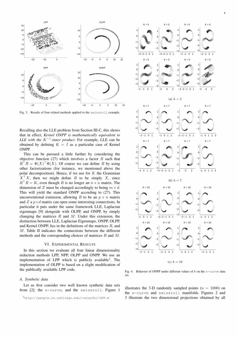
Fig. 3. Results of four related methods applied to the swissroll example.

Recalling also the LLE problem from Section III-C, this showsthat in effect, Kernel ONPP is mathematically equivalent toLLE with the K−1-inner product. For example, LLE can beobtained by defining K = I as a particular case of KernelONPP.

This can be pursued a little further by considering theobjective function (27) which involves a factor R such thatR>R = Φ(X)>Φ(X). Of course we can define R by usingother factorizations (for instance, we mentioned above thepolar decomposition). Hence, if we use for K the GrammianX>X , then we might define R to be simply X , sinceR>R = K, even though R is no longer an n×n matrix. Thedimension of Z must be changed accordingly to being m×d.This will yield the standard ONPP according to (27). Thisunconventional extension, allowing R to be an p × n matrixand Z a p×d matrix can open some interesting connections. Inparticular it puts under the same framework LLE, Laplacianeigenmaps [9] alongside with OLPP, and ONPP, by simplychanging the matrices R and M . Under this extension, thedistinction between LLE, Laplacian Eigenmaps, ONPP, OLPP,and Kernel ONPP, lies in the definitions of the matrices R, andM . Table II indicates the connections between the differentmethods and the corresponding choices of matrices R and M .

VI. EXPERIMENTAL RESULTS

In this section we evaluate all four linear dimensionalityreduction methods LPP, NPP, OLPP and ONPP. We use animplementation of LPP which is publicly available1. Theimplementation of OLPP is based on a slight modification ofthe publically available LPP code.

A. Synthetic data

Let us first consider two well known synthetic data setsfrom [2]: the s-curve, and the swissroll. Figure 1

1http://people.cs.uchicago.edu/∼xiaofei/LPP.m

−3 −2 −1 0 1

−2

−1

0

1

K = 5

−3−2 −1 0 1

−2

−1

0

1

K = 5

−2 −1 0 1−3

−2

−1

0

1

K = 5

−2 −1 0 1

−3

−2

−1

0

1

K = 5

−2 −1 0 1

−3

−2

−1

0

1

K = 5

−2 0 2−3

−2

−1

0

1

K = 5

−3 −2 −1 0 1

−3

−2

−1

0

1

K = 5

−4 −2 0

−3

−2

−1

0

1

K = 5

(a) k = 5

−2 −1 0 1

−2

−1

0

1

K = 7

−1 0 1 2

−2

−1

0

1

K = 7

−3 −2 −1 0 1

−2

−1

0

1

K = 7

−1 0 1 2 3

−2

−1

0

1

K = 7

−1 0 1 2

−2

−1

0

1

K = 7

−3 −2 −1 0 1−3

−2

−1

0

1

K = 7

−2 0 2

−2

−1

0

1

K = 7

−1 0 1 2 3

−2

−1

0

1

K = 7

(b) k = 7

−1 0 1 2

−2

−1

0

1

K = 10

−3 −2 −1 0 1

−2

−1

0

1

K = 10

−2 −1 0 1−3

−2

−1

0

1

K = 10

−1 0 1 2

−2

−1

0

1

K = 10

−2 −1 0 1−3

−2

−1

0

1

K = 10

−2 −1 0 1

−2

−1

0

1

K = 10

−1 0 1 2

−2

−1

0

1

K = 10

−2 −1 0 1

−2

−1

0

1

K = 10

(c) k = 10

Fig. 4. Behavior of ONPP under different values of k on the s-curve dataset.

illustrates the 3-D randomly sampled points (n = 1000) onthe s-curve and swissroll manifolds. Figures 2 and3 illustrate the two dimensional projections obtained by all

9

−10 0 10−15

−10

−5

0

5

10

K = 5

−10 0 10−15

−10

−5

0

5

10

K = 5

−10 0 10

−10

0

10

K = 5

−10 0 10−15

−10

−5

0

5

10

K = 5

−10 0 10

−15

−10

−5

0

5

10

K = 5

−10 0 10 20−15

−10

−5

0

5

10

K = 5

−10 0 10

−15

−10

−5

0

5

10

K = 5

−10 0 10

−15

−10

−5

0

5

10

K = 5

(a) k = 5

−10 0 10−15

−10

−5

0

5

10

K = 7

−10 0 10−15

−10

−5

0

5

10

K = 7

−10 0 10

−10

0

10

K = 7

−10 0 10−15

−10

−5

0

5

10

K = 7

−10 0 10

−15

−10

−5

0

5

10

K = 7

−10 0 10

−10

−5

0

5

10

15

K = 7

−10 0 10−15

−10

−5

0

5

10

K = 7

−10 0 10

−15

−10

−5

0

5

10

K = 7

(b) k = 7

−10 0 10−15

−10

−5

0

5

10

K = 10

−10 0 10−15

−10

−5

0

5

10

K = 10

−10 0 10−15

−10

−5

0

5

10

K = 10

−10 0 10

−15

−10

−5

0

5

10

K = 10

−10 0 10−15

−10

−5

0

5

10

K = 10

−10 0 10

−15

−10

−5

0

5

10

K = 10

−10 0 10−15

−10

−5

0

5

10

K = 10

−10 0 10−15

−10

−5

0

5

10

K = 10

(c) k = 10

Fig. 5. Behavior of ONPP under different values of k on the swissrolldata set.

methods in the s-curve and swissroll data sets. Theaffinity graphs were all constructed using k = 10 nearestneighbor points. Observe that the performance of LPP parallels

Method Matrix M Matrix R

LLE (I −W>a )(I −Wa) I

Laplacian Eigenmaps (D −W>L ) I

ONPP (I −W>a )(I −Wa) X

OLPP (D −W>L ) X

K-ONPP with Kernel K (I −W>)(I −W ) R>R = K (Chol.)

TABLE IIDIFFERENT METHODS AND THE CORRESPONDING CHOICES FOR THE

MATRICES R AND M . THE MATRIX Wa CORRESPONDS TO THE AFFINITY

GRAPH IN LLE AND ONPP, SEE SECTION III-A FOR DETAILS. THE

MATRIX D −WL IS THE LAPLACIAN GRAPH USED IN LAPLACIAN

EIGENMAPS AND OLPP, SEE SEC. II-A AND [9], [8] FOR DETAILS.

that of NPP and, similarly, the performance of OLPP parallelsthat of ONPP. Note that all methods preserve locality whichis indicated by the gray scale darkness value. However, theorthogonal methods i.e., OLPP and ONPP preserve globalgeometric characteristics as well, since they give faithfulprojections which convey information about how the manifoldis folded in the high dimensional space. This may be the resultof the great overlap among the neighbor sets of data samplesthat are close by.

Figures 4 and 5 illustrate the sensitivity of ONPP withrespect to random realizations of the data set, for differentvalues of k, for the s-curve and the swissroll manifoldsrespectively. We test with a few representative values of kand we compute eight projections for eight different randomrealizations of the data sets. The number of samples was setto n = 1000. Notice that when k is small, the k-NN graph isnot able to capture effectively the geometry of the data set. Insome cases this results in the method yielding slightly differentprojections for different realizations of the data set. However,as k increases, the k-NN graph captures more effectively thedata geometry and ONPP yields a stable result across thedifferent realizations of the data set.

B. Digit visualization

The next experiment involves digit visualization. We use20 × 16 images of handwritten digits which are publicallyavailable from S. Roweis’ web page2. The data set contains 39samples from each class (digits from ’0’-’9’). Each digit imagesample is represented lexicographically as a high dimensionalvector of length 320. For the purpose of comparison with PCA,we first project the data set in the two dimensional space usingPCA and the results are depicted in Figure 6. In the sequel weproject the data set in two dimensions using all four methods.The results are illustrated in Figures 7 (digits ’0’-’4’) and 8(digits ’5’-’9’). We use k = 6 for constructing the affinitygraphs of all methods.

Observe that the projections of PCA are spread out sincePCA aims at maximizing the variance. However, the classesof different digits seem to heavily overlap. This means thatPCA is not well suited for discriminating between data. Onthe other hand, observe that all the four graph-based methods

2http://www.cs.toronto.edu/∼roweis/data.html

10

−15 −10 −5 0−8

−6

−4

−2

0

2

4PCA, digits: 0−4

−5 0 5 10−4

−2

0

2

4

6

8PCA, digits: 5−9

Fig. 6. Two dimensional projections of digits using PCA. Left panel: ‘+’ denotes 0, ‘x’ denotes 1, ‘o’ denotes 2, ‘4’ denotes 3 and ‘¤’ denotes 4. Rightpanel: ‘+’ denotes 5, ‘x’ denotes 6, ‘o’ denotes 7, ‘4’ denotes 8 and ‘¤’ denotes 9.

−0.5 0 0.5 1−1

−0.5

0

0.5

1NPP, digits: 0−4

−0.5 0 0.5 1 1.5−2

−1.5

−1

−0.5

0ONPP, digits: 0−4

0.5 1 1.5 2 2.5 3−0.6

−0.4

−0.2

0

0.2

0.4

0.6

0.8

1LPP, digits: 0−4

−0.4 −0.2 0 0.2 0.4 0.6−0.3

−0.2

−0.1

0

0.1

0.2

0.3

0.4OLPP, digits: 0−4

Fig. 7. Two dimensional projections of digits using four related methods, where ‘+’ denotes 0, ‘x’ denotes 1, ‘o’ denotes 2, ‘4’ denotes 3 and ‘¤’ denotes4.

yield more meaningful projections since samples of the sameclass are mapped close to each other. This is because thesemethods aim at preserving locality. Finally, ONPP seems toprovide slightly better projections than the other methods sinceits clusters appear more cohesive.

C. Face recognition

In this section we evaluate all methods for the problem offace recognition. We used three data sets which are publically

available: UMIST [13], ORL [14] and AR [15]. The size ofthe images is 112×92 in all data sets. As is common practicethe images in all databases were downsampled to size 38×31,for computational efficiency. Thus, each facial image wasrepresented lexicographically as a high dimensional vector oflength 1,178. In order to measure the recognition performance,we use a random subset of facial expressions/poses from eachsubject as training set and the remaining as test set. Thetest samples are projected in the reduced space using the

11

−2 −1.5 −1 −0.5 0 0.5−1.5

−1

−0.5

0

0.5

1NPP, digits: 5−9

−1.5 −1 −0.5 0 0.5 1−2

−1.5

−1

−0.5

0

0.5

1ONPP, digits: 5−9

−2.5 −2 −1.5 −1 −0.5−1

−0.5

0

0.5

1

1.5

2LPP, digits: 5−9

−0.2 0 0.2 0.4 0.6−0.4

−0.2

0

0.2

0.4

0.6

0.8

1OLPP, digits: 5−9

Fig. 8. Two dimensional projections of digits using four related methods, ‘+’ denotes 5, ‘x’ denotes 6, ‘o’ denotes 7, ‘4’ denotes 8 and ‘¤’ denotes 9.

Fig. 9. Sample face images from the UMIST database. The number ofdifferent poses poses for each subject is varying.

Fig. 10. Sample face images from the ORL database. There are 10 availablefacial expressions and poses for each subject.

dimensionality reduction matrix V which is learned from thetraining samples. Then, recognition is performed in the lowdimensional space using nearest-neighbor (NN) classification.In order to ensure that our results are not biased from aspecific random realization of the training/test set, we perform20 different random realizations of the training/test sets andwe report the average error rate.

We also compare all four methods with Fisherfaces [16],a well known method for face recognition. Fisherfaces isa supervised method which determines V by using LinearDiscriminant Analysis (LDA). LDA works by extracting a

Fig. 11. Sample face images from the AR database. Facial expressions fromleft to right: ‘natural expression’, ‘smile’, ‘anger’, ‘scream’, ‘left light on’,‘right light on’, ‘all side lights on’ and ‘wearing sun glasses’.

set of “optimal” discriminating axes. Assume that we have cclasses and that class i has ni data points. Define the between-class scatter matrix

SB =c∑

i=1

ni(µ(i) − µ)(µ(i) − µ)>

and the within-class scatter matrix

SW =c∑

i=1

ni∑

j=1

(x(i)j − µ(i))(x(i)

j − µ(i))>

where µ(i) is the centroid of the i-th class and µ the globalcentroid. In LDA the columns of V are the eigenvectors asso-ciated with largest eigenvalues of the generalized eigenvalueproblem

SBw = λSW w. (33)

12

10 20 30 40 50 60 700

2

4

6

8

10

12

14UMIST

dimension of reduced space

erro

r ra

te (

%) LPP

OLPPPCAONPPNPPLDA

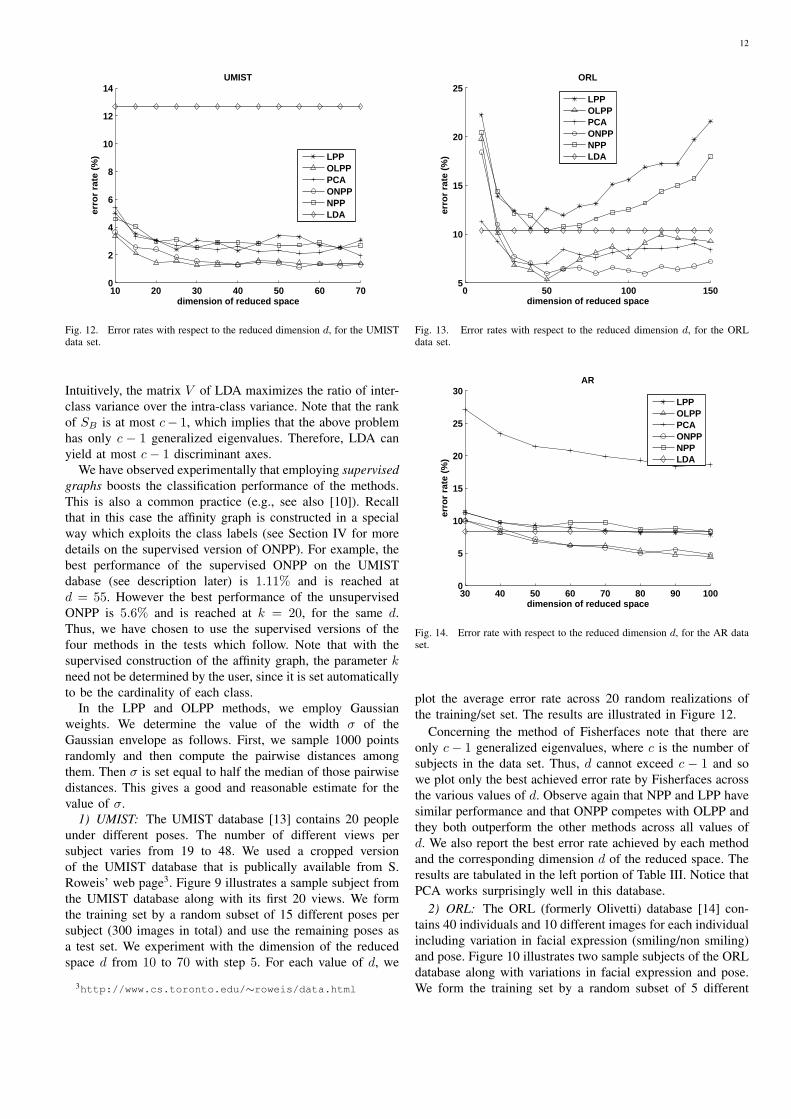
Fig. 12. Error rates with respect to the reduced dimension d, for the UMISTdata set.

Intuitively, the matrix V of LDA maximizes the ratio of inter-class variance over the intra-class variance. Note that the rankof SB is at most c− 1, which implies that the above problemhas only c − 1 generalized eigenvalues. Therefore, LDA canyield at most c− 1 discriminant axes.

We have observed experimentally that employing supervisedgraphs boosts the classification performance of the methods.This is also a common practice (e.g., see also [10]). Recallthat in this case the affinity graph is constructed in a specialway which exploits the class labels (see Section IV for moredetails on the supervised version of ONPP). For example, thebest performance of the supervised ONPP on the UMISTdabase (see description later) is 1.11% and is reached atd = 55. However the best performance of the unsupervisedONPP is 5.6% and is reached at k = 20, for the same d.Thus, we have chosen to use the supervised versions of thefour methods in the tests which follow. Note that with thesupervised construction of the affinity graph, the parameter kneed not be determined by the user, since it is set automaticallyto be the cardinality of each class.

In the LPP and OLPP methods, we employ Gaussianweights. We determine the value of the width σ of theGaussian envelope as follows. First, we sample 1000 pointsrandomly and then compute the pairwise distances amongthem. Then σ is set equal to half the median of those pairwisedistances. This gives a good and reasonable estimate for thevalue of σ.

1) UMIST: The UMIST database [13] contains 20 peopleunder different poses. The number of different views persubject varies from 19 to 48. We used a cropped versionof the UMIST database that is publically available from S.Roweis’ web page3. Figure 9 illustrates a sample subject fromthe UMIST database along with its first 20 views. We formthe training set by a random subset of 15 different poses persubject (300 images in total) and use the remaining poses asa test set. We experiment with the dimension of the reducedspace d from 10 to 70 with step 5. For each value of d, we

3http://www.cs.toronto.edu/∼roweis/data.html

0 50 100 1505

10

15

20

25ORL

dimension of reduced space

erro

r ra

te (

%)

LPPOLPPPCAONPPNPPLDA

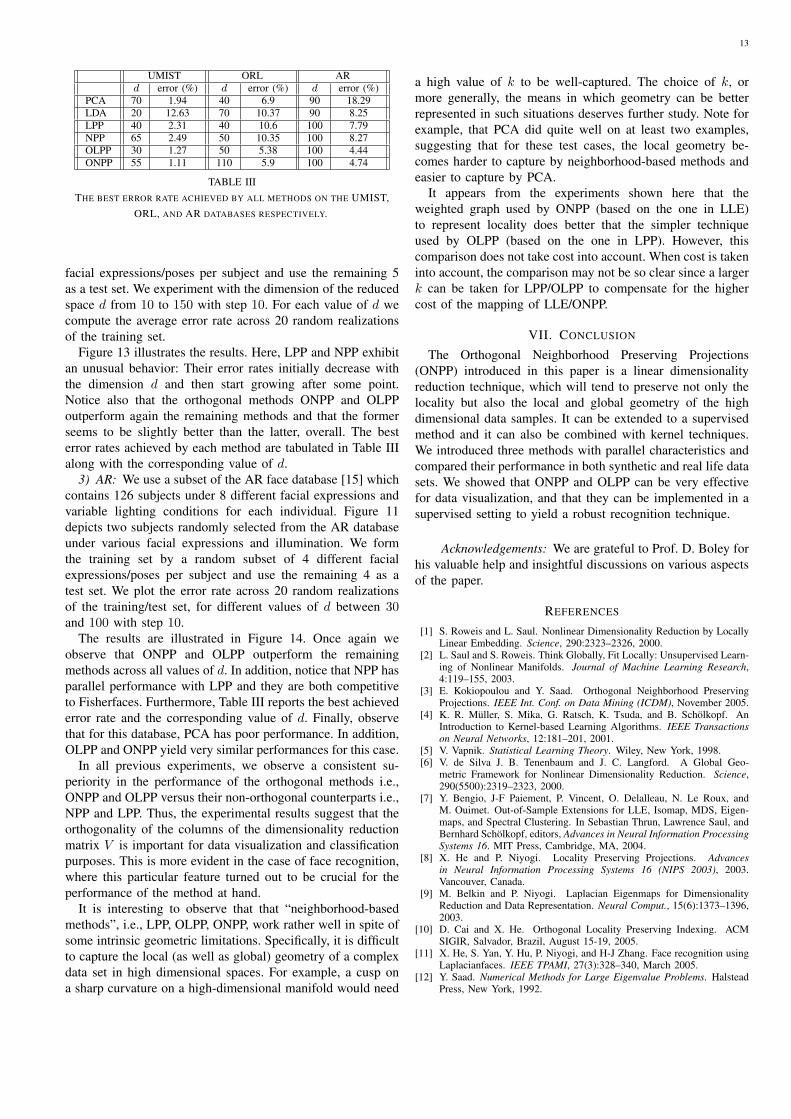
Fig. 13. Error rates with respect to the reduced dimension d, for the ORLdata set.

30 40 50 60 70 80 90 1000

5

10

15

20

25

30AR

dimension of reduced space

erro

r ra

te (

%)

LPPOLPPPCAONPPNPPLDA

Fig. 14. Error rate with respect to the reduced dimension d, for the AR dataset.

plot the average error rate across 20 random realizations ofthe training/set set. The results are illustrated in Figure 12.

Concerning the method of Fisherfaces note that there areonly c− 1 generalized eigenvalues, where c is the number ofsubjects in the data set. Thus, d cannot exceed c − 1 and sowe plot only the best achieved error rate by Fisherfaces acrossthe various values of d. Observe again that NPP and LPP havesimilar performance and that ONPP competes with OLPP andthey both outperform the other methods across all values ofd. We also report the best error rate achieved by each methodand the corresponding dimension d of the reduced space. Theresults are tabulated in the left portion of Table III. Notice thatPCA works surprisingly well in this database.

2) ORL: The ORL (formerly Olivetti) database [14] con-tains 40 individuals and 10 different images for each individualincluding variation in facial expression (smiling/non smiling)and pose. Figure 10 illustrates two sample subjects of the ORLdatabase along with variations in facial expression and pose.We form the training set by a random subset of 5 different

13

UMIST ORL ARd error (%) d error (%) d error (%)

PCA 70 1.94 40 6.9 90 18.29LDA 20 12.63 70 10.37 90 8.25LPP 40 2.31 40 10.6 100 7.79NPP 65 2.49 50 10.35 100 8.27OLPP 30 1.27 50 5.38 100 4.44ONPP 55 1.11 110 5.9 100 4.74

TABLE IIITHE BEST ERROR RATE ACHIEVED BY ALL METHODS ON THE UMIST,

ORL, AND AR DATABASES RESPECTIVELY.

facial expressions/poses per subject and use the remaining 5as a test set. We experiment with the dimension of the reducedspace d from 10 to 150 with step 10. For each value of d wecompute the average error rate across 20 random realizationsof the training set.

Figure 13 illustrates the results. Here, LPP and NPP exhibitan unusual behavior: Their error rates initially decrease withthe dimension d and then start growing after some point.Notice also that the orthogonal methods ONPP and OLPPoutperform again the remaining methods and that the formerseems to be slightly better than the latter, overall. The besterror rates achieved by each method are tabulated in Table IIIalong with the corresponding value of d.

3) AR: We use a subset of the AR face database [15] whichcontains 126 subjects under 8 different facial expressions andvariable lighting conditions for each individual. Figure 11depicts two subjects randomly selected from the AR databaseunder various facial expressions and illumination. We formthe training set by a random subset of 4 different facialexpressions/poses per subject and use the remaining 4 as atest set. We plot the error rate across 20 random realizationsof the training/test set, for different values of d between 30and 100 with step 10.

The results are illustrated in Figure 14. Once again weobserve that ONPP and OLPP outperform the remainingmethods across all values of d. In addition, notice that NPP hasparallel performance with LPP and they are both competitiveto Fisherfaces. Furthermore, Table III reports the best achievederror rate and the corresponding value of d. Finally, observethat for this database, PCA has poor performance. In addition,OLPP and ONPP yield very similar performances for this case.

In all previous experiments, we observe a consistent su-periority in the performance of the orthogonal methods i.e.,ONPP and OLPP versus their non-orthogonal counterparts i.e.,NPP and LPP. Thus, the experimental results suggest that theorthogonality of the columns of the dimensionality reductionmatrix V is important for data visualization and classificationpurposes. This is more evident in the case of face recognition,where this particular feature turned out to be crucial for theperformance of the method at hand.

It is interesting to observe that that “neighborhood-basedmethods”, i.e., LPP, OLPP, ONPP, work rather well in spite ofsome intrinsic geometric limitations. Specifically, it is difficultto capture the local (as well as global) geometry of a complexdata set in high dimensional spaces. For example, a cusp ona sharp curvature on a high-dimensional manifold would need

a high value of k to be well-captured. The choice of k, ormore generally, the means in which geometry can be betterrepresented in such situations deserves further study. Note forexample, that PCA did quite well on at least two examples,suggesting that for these test cases, the local geometry be-comes harder to capture by neighborhood-based methods andeasier to capture by PCA.

It appears from the experiments shown here that theweighted graph used by ONPP (based on the one in LLE)to represent locality does better that the simpler techniqueused by OLPP (based on the one in LPP). However, thiscomparison does not take cost into account. When cost is takeninto account, the comparison may not be so clear since a largerk can be taken for LPP/OLPP to compensate for the highercost of the mapping of LLE/ONPP.

VII. CONCLUSION

The Orthogonal Neighborhood Preserving Projections(ONPP) introduced in this paper is a linear dimensionalityreduction technique, which will tend to preserve not only thelocality but also the local and global geometry of the highdimensional data samples. It can be extended to a supervisedmethod and it can also be combined with kernel techniques.We introduced three methods with parallel characteristics andcompared their performance in both synthetic and real life datasets. We showed that ONPP and OLPP can be very effectivefor data visualization, and that they can be implemented in asupervised setting to yield a robust recognition technique.

Acknowledgements: We are grateful to Prof. D. Boley forhis valuable help and insightful discussions on various aspectsof the paper.

REFERENCES

[1] S. Roweis and L. Saul. Nonlinear Dimensionality Reduction by LocallyLinear Embedding. Science, 290:2323–2326, 2000.

[2] L. Saul and S. Roweis. Think Globally, Fit Locally: Unsupervised Learn-ing of Nonlinear Manifolds. Journal of Machine Learning Research,4:119–155, 2003.

[3] E. Kokiopoulou and Y. Saad. Orthogonal Neighborhood PreservingProjections. IEEE Int. Conf. on Data Mining (ICDM), November 2005.

[4] K. R. Muller, S. Mika, G. Ratsch, K. Tsuda, and B. Scholkopf. AnIntroduction to Kernel-based Learning Algorithms. IEEE Transactionson Neural Networks, 12:181–201, 2001.

[5] V. Vapnik. Statistical Learning Theory. Wiley, New York, 1998.[6] V. de Silva J. B. Tenenbaum and J. C. Langford. A Global Geo-

metric Framework for Nonlinear Dimensionality Reduction. Science,290(5500):2319–2323, 2000.

[7] Y. Bengio, J-F Paiement, P. Vincent, O. Delalleau, N. Le Roux, andM. Ouimet. Out-of-Sample Extensions for LLE, Isomap, MDS, Eigen-maps, and Spectral Clustering. In Sebastian Thrun, Lawrence Saul, andBernhard Scholkopf, editors, Advances in Neural Information ProcessingSystems 16. MIT Press, Cambridge, MA, 2004.

[8] X. He and P. Niyogi. Locality Preserving Projections. Advancesin Neural Information Processing Systems 16 (NIPS 2003), 2003.Vancouver, Canada.

[9] M. Belkin and P. Niyogi. Laplacian Eigenmaps for DimensionalityReduction and Data Representation. Neural Comput., 15(6):1373–1396,2003.

[10] D. Cai and X. He. Orthogonal Locality Preserving Indexing. ACMSIGIR, Salvador, Brazil, August 15-19, 2005.

[11] X. He, S. Yan, Y. Hu, P. Niyogi, and H-J Zhang. Face recognition usingLaplacianfaces. IEEE TPAMI, 27(3):328–340, March 2005.

[12] Y. Saad. Numerical Methods for Large Eigenvalue Problems. HalsteadPress, New York, 1992.

14

[13] D. B Graham and N. M Allinson. Characterizing Virtual Eigensignaturesfor General Purpose Face Recognition. Face Recognition: From Theoryto Applications, 163:446–456, 1998.

[14] F. Samaria and A. Harter. Parameterisation of a Stochastic Model forHuman Face Identification. In 2nd IEEE Workshop on Applications ofComputer Vision, Sarasota FL, December 1994.

[15] A.M. Martinez and R. Benavente. The AR Face Database. Technicalreport, CVC no. 24, 1998.

[16] P. Belhumeur, J. Hespanha, and D. Kriegman. Eigenfaces vs. Fish-erfaces: Recognition Using Class Specific Linear Projection. IEEETrans. Pattern Analysis and Machine Intelligence, Special Issue on FaceRecognition, 19(7):711—20, July 1997.

Effrosyni Kokiopoulou received her Diploma inEngineering in June 2002, from the Computer Engi-neering and Informatics Department of the Univer-sity of Patras, Greece. In June 2005, she received aMsc degree in Computer Science from the ComputerScience and Engineering Department of the Univer-sity of Minnesota, USA, under the supervision ofprof. Yousef Saad. In September 2005, she joinedthe LTS4 Lab of the Signal Processing Institute, inthe Swiss Federal Institute of Technology (EPFL),Lausanne, Switzerland. She is currently working

towards her PhD degree under the supervision of prof. Pascal Frossard. Herresearch interests include multimedia data mining, machine learning, computervision and numerical linear algebra. She is a student member of the IEEE.

Yousef Saad Yousef Saad is an Institute of Tech-nology (I.T.) distinguished professor with the de-partment of computer science and engineering at theUniversity of Minnesota. He received the ”Doctoratd’Etat” from the university of Grenoble (France) in1983. He joined the university of Minnesota in 1990as a Professor of computer science and a Fellowof the Minnesota Supercomputer Institute. He washead of the department of Computer Science andEngineering from January 1997 to June 2000, andbecame an IT distinguished professor in May 2005.

From 1981 to 1990, he held positions at the University of California atBerkeley, Yale, the University of Illinois, and the Research Institute forAdvanced Computer Science (RIACS). His current research interests include:numerical linear algebra, sparse matrix computations, iterative methods, par-allel computing, numerical methods for electronic structure, and data analysis.He is the author of two (single authored) books and over 120 journal articles.He is also the developer or co-developer of several software packages forsolving sparse linear systems of equations including SPARSKIT, pARMS,and ITSOL.