Embed Size (px)
Citation preview
Motivation and IntroductionA Property Rights Model in a Sequential Production Setting
Empirical Evidence
Organizing the Global Value Chain
Pol Antras Davin Chor
Harvard SMU
9-12 July 2012
NBER SI
Pol Antras Davin Chor Organizing the Global Value Chain
Motivation and IntroductionA Property Rights Model in a Sequential Production Setting
Empirical Evidence
Motivation and Introduction
Many production processes are sequential in nature:
I Raw materials processing −→ Basic components
−→ Complex assembly −→ Sales and Distribution
I Downstream stages often cannot commence before upstream stages
I Classic motivating example: Henry Ford’s Model T production line
I More recently: Sequential production processes now often fragmentedacross country borders
I Existing literature: On the consequences of sequential location decisions
I This paper: What is the optimal way to organize production along suchglobal sequential production processes?
Pol Antras Davin Chor Organizing the Global Value Chain

Motivation and IntroductionA Property Rights Model in a Sequential Production Setting
Empirical Evidence
Motivation and Introduction
Our premise: Contractual frictions matter for the organizational decisions offirms over particular production stages
Example: The Boeing Dreamliner
I Repeated delays led to reorganization of the sourcing model
I In 2008-09, Boeing successively acquired Vought Aircraft Industries’operations in South Carolina, which were producing rear sections of theDreamliner’s fuselage
I Culminated in a full buyout in Jul 2009:
“The 787’s entry into service has been set back five times, inpart because multiple suppliers didn’t do all the work they hadagreed to, leaving more for Boeing workers to complete.”
Source: http://www.bloomberg.com/apps/news?pid=newsarchive&sid=aF6uWvMb9C08
Pol Antras Davin Chor Organizing the Global Value Chain

Motivation and IntroductionA Property Rights Model in a Sequential Production Setting
Empirical Evidence
Some Questions
I Why does the firm not bring the whole production process within its firmboundaries?
I What determines which suppliers are brought inside the firm and which arenot, and why might “downstreamness” matter for this?
I Property-rights theory (Grossman and Hart, 1986, Hart and Moore, 1990)provides the most convincing framework to answer the first question...
I ... so it seems a natural approach to use to tackle the second question aswell
Pol Antras Davin Chor Organizing the Global Value Chain

Motivation and IntroductionA Property Rights Model in a Sequential Production Setting
Empirical Evidence
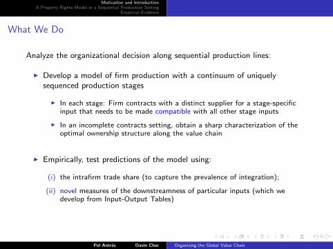
What We Do
Analyze the organizational decision along sequential production lines:
I Develop a model of firm production with a continuum of uniquelysequenced production stages
I In each stage: Firm contracts with a distinct supplier for a stage-specificinput that needs to be made compatible with all other stage inputs
I In an incomplete contracts setting, obtain a sharp characterization of theoptimal ownership structure along the value chain
I Empirically, test predictions of the model using:
(i) the intrafirm trade share (to capture the prevalence of integration);
(ii) novel measures of the downstreamness of particular inputs (which wedevelop from Input-Output Tables)
Pol Antras Davin Chor Organizing the Global Value Chain
Motivation and IntroductionA Property Rights Model in a Sequential Production Setting
Empirical Evidence
What We Do
Analyze the organizational decision along sequential production lines:
I Develop a model of firm production with a continuum of uniquelysequenced production stages
I In each stage: Firm contracts with a distinct supplier for a stage-specificinput that needs to be made compatible with all other stage inputs
I In an incomplete contracts setting, obtain a sharp characterization of theoptimal ownership structure along the value chain
I Empirically, test predictions of the model using:
(i) the intrafirm trade share (to capture the prevalence of integration);
(ii) novel measures of the downstreamness of particular inputs (which wedevelop from Input-Output Tables)
Pol Antras Davin Chor Organizing the Global Value Chain

Motivation and IntroductionA Property Rights Model in a Sequential Production Setting
Empirical Evidence
Related Literature
1. Sequential production
I Eg: Findlay (1978), Dixit and Grossman (1982), Sanyal (1983), Kremer(1993), Yi (2003), Harms, Lorz, and Urban (2009), Baldwin and Venables(2010), Costinot et al. (2011)
I Small literature on incentives in sequential production processes. Eg:Winter (2006), Kim and Shin (2011)
2. Property rights theory of the firm in international trade
I Eg: Grossman and Helpman (2002, 2005), Antras (2003), Antras andHelpman (2004, 2008)
3. Empirical evidence (determinants of the intrafirm trade share)
I Eg: Antras (2003), Tomiura (2007), Defever and Toubal (2007), Nunn andTrefler (2008a,b), Corcos et al. (2009), Dıez (2010), Bernard et al. (2010),Kohler and Smolka (2010)
Pol Antras Davin Chor Organizing the Global Value Chain

Motivation and IntroductionA Property Rights Model in a Sequential Production Setting
Empirical Evidence
Setup of the ModelKey PredictionsExtensions
Plan of Talk
1. Motivation and Introduction
2. Setup of the Core Model
3. Key Predictions
4. Extensions
5. Empirical Evidence
6. Conclusion
Pol Antras Davin Chor Organizing the Global Value Chain

Motivation and IntroductionA Property Rights Model in a Sequential Production Setting
Empirical Evidence
Setup of the ModelKey PredictionsExtensions
Basic Setup: Production Function
I Production requires the completion of a continuum of stages indexed byj ∈ [0, 1]
I Unique sequence of stages: j increasing as production moves downstream
I Let x(j) be the services of compatible intermediate inputs that supplier jdelivers to the Firm. Quality-adjusted volume of final-good production is
q = θ
(∫ 1
0
x(j)αI (j) dj
)1/α
, (1)
I (j) =
1 if input j is produced after all inputs j ′ < j
0 otherwise
I α ∈ (0, 1): captures how substitutable the stage inputs are
I θ: firm productivity parameter
Pol Antras Davin Chor Organizing the Global Value Chain
Motivation and IntroductionA Property Rights Model in a Sequential Production Setting
Empirical Evidence
Setup of the ModelKey PredictionsExtensions
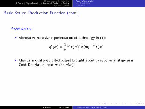
Basic Setup: Production Function (cont.)
Short remark:
I Alternative recursive representation of technology in (1):
q′ (m) =1
αθαx(m)αq (m)1−α I (m)
I Change in quality-adjusted output brought about by supplier at stage m isCobb-Douglas in input m and q(m)
Pol Antras Davin Chor Organizing the Global Value Chain
Motivation and IntroductionA Property Rights Model in a Sequential Production Setting
Empirical Evidence
Setup of the ModelKey PredictionsExtensions
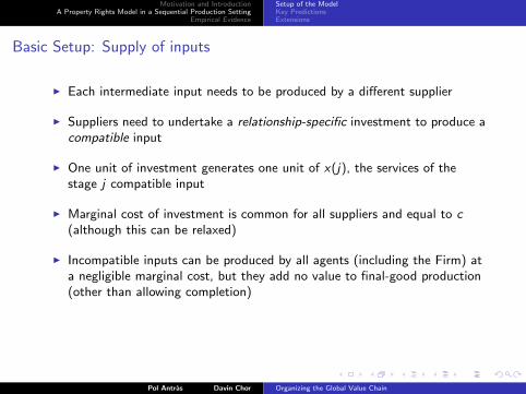
Basic Setup: Supply of inputs
I Each intermediate input needs to be produced by a different supplier
I Suppliers need to undertake a relationship-specific investment to produce acompatible input
I One unit of investment generates one unit of x(j), the services of thestage j compatible input
I Marginal cost of investment is common for all suppliers and equal to c(although this can be relaxed)
I Incompatible inputs can be produced by all agents (including the Firm) ata negligible marginal cost, but they add no value to final-good production(other than allowing completion)
Pol Antras Davin Chor Organizing the Global Value Chain

Motivation and IntroductionA Property Rights Model in a Sequential Production Setting
Empirical Evidence
Setup of the ModelKey PredictionsExtensions
Basic Setup: Final good demand
I Consumers have preferences:
U =
(∫ω∈Ω
(ϕ (ω) q (ω))ρ dω
)1/ρ
, with ρ ∈ (0, 1) (2)
I ϕ (ω): quality of a variety
I q (ω): consumption in physical units
I Implied revenue function of any firm in the industry is concave inquality-adjusted output q (ω) = ϕ (ω) q (ω) with a constant elasticity ρ:
r = A1−ρqρ = A1−ρθρ(∫ 1
0
x (j)α dj
)ρ/α(3)
Pol Antras Davin Chor Organizing the Global Value Chain
Motivation and IntroductionA Property Rights Model in a Sequential Production Setting
Empirical Evidence
Setup of the ModelKey PredictionsExtensions
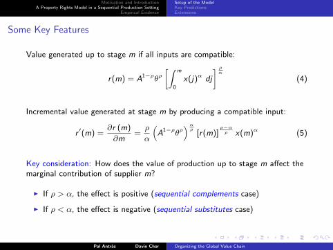
Some Key Features
Value generated up to stage m if all inputs are compatible:
r(m) = A1−ρθρ[∫ m
0
x(j)α dj
] ρα
(4)
Incremental value generated at stage m by producing a compatible input:
r ′(m) =∂r (m)
∂m=ρ
α
(A1−ρθρ
)αρ
[r(m)]ρ−α
ρ x(m)α (5)
Key consideration: How does the value of production up to stage m affect themarginal contribution of supplier m?
I If ρ > α, the effect is positive (sequential complements case)
I If ρ < α, the effect is negative (sequential substitutes case)
Pol Antras Davin Chor Organizing the Global Value Chain
Motivation and IntroductionA Property Rights Model in a Sequential Production Setting
Empirical Evidence
Setup of the ModelKey PredictionsExtensions
Some Key Features (cont.)
Why does ρ matter?
I From a technological point of view, all inputs are complements sinceα ∈ (0, 1)
I But when ρ is small, firm faces an inelastic demand function, so marginalrevenue falls quickly with quality-adjusted output
I Large investments prior to stage m therefore discourage supplier effort atstage m
I It turns out that when ρ < α, this revenue effect is strong enough todominate the physical input complementarity effect
Pol Antras Davin Chor Organizing the Global Value Chain

Motivation and IntroductionA Property Rights Model in a Sequential Production Setting
Empirical Evidence
Setup of the ModelKey PredictionsExtensions
Benchmark: Complete Contracts
If contracting frictions are absent, firm signs a contract with each input supplierspecifying the optimal quantity of compatible inputs, x(j), to maximize:
πF = A1−ρθρ(∫ 1
0
x(j)αdj
) ρα
− c
∫ 1
0
x(j)dj (6)
Solution entails:
I A common investment level, x =(ρA1−ρθρ/c
)1/(1−ρ), for all inputs j
I Suppliers are paid their marginal cost: cx
I Even though
r ′(m) =∂r (m)
∂m=ρ
α
(A1−ρθρ
)αρ
[r(m)]ρ−α
ρ x(m)α,
the Firm internalizes the downstream effects of upstream investments
Pol Antras Davin Chor Organizing the Global Value Chain

Motivation and IntroductionA Property Rights Model in a Sequential Production Setting
Empirical Evidence
Setup of the ModelKey PredictionsExtensions
Incomplete Contracting
Suppose that the environment is one of incomplete contracts
I Compatibility cannot be verified and enforced by a third-party court
I But Firm and suppliers have symmetric information regarding compatibility
I Contracts contingent on total revenue are not useful in our context
I Abstract from mechanisms
I Suppliers’ payoffs are determined in ex post (re)-negotiation, after x(m)has been produced
Pol Antras Davin Chor Organizing the Global Value Chain

Motivation and IntroductionA Property Rights Model in a Sequential Production Setting
Empirical Evidence
Setup of the ModelKey PredictionsExtensions
Bargaining
I Supplier m and Firm engage in generalized Nash bargaining over theincremental value contribution made by supplier m, r ′(m)
I Supplier m’s outside option normalized to 0
I Under integration, Firm’s control rights tilt the ex-post division of surplusin its favor relative to under outsourcing (as in Grossman and Hart, 1986).
I Let β (m) be the share of r ′(m) that accrues to the firm in the bargain:
β (m) =
βO if the firm outsources stage m
βV > βO if the firm integrates stage m
Pol Antras Davin Chor Organizing the Global Value Chain

Motivation and IntroductionA Property Rights Model in a Sequential Production Setting
Empirical Evidence
Setup of the ModelKey PredictionsExtensions
Timing
1. Firm posts contracts for suppliers for each stage j ∈ [0, 1], stating theorganizational mode (integration vs outsourcing).
2. Suppliers apply. Firm chooses one supplier for each stage j .
3. Production takes place sequentially. The supplier chooses x(m) afterobserving the value of r(m).
4. At the end of stage m, the supplier and Firm bargain over r ′(m). Firmpays the supplier.
5. Total revenue, A1−ρqρ, ρ ∈ (0, 1), from the sale of the final good iscollected by the Firm.
Pol Antras Davin Chor Organizing the Global Value Chain

Motivation and IntroductionA Property Rights Model in a Sequential Production Setting
Empirical Evidence
Setup of the ModelKey PredictionsExtensions
Discussion
I Bargaining is over supplier’s marginal contribution at stage m, not itsultimate (or average marginal) contribution
I Can be rationalized by limited commitment frictions: Hart and Moore(1994), Thomas and Worrall (1994)
I Supplier does not want to delay receiving payment; or Firm might beconstrained in borrowing more than r ′(m)
I Note: Results surprisingly robust to alternative bargaining protocols
Pol Antras Davin Chor Organizing the Global Value Chain

Motivation and IntroductionA Property Rights Model in a Sequential Production Setting
Empirical Evidence
Setup of the ModelKey PredictionsExtensions
Plan of Talk
1. Motivation and Introduction
2. Setup of the Core Model
3. Key Predictions
4. Extensions
5. Empirical Evidence
6. Conclusion
Pol Antras Davin Chor Organizing the Global Value Chain

Motivation and IntroductionA Property Rights Model in a Sequential Production Setting
Empirical Evidence
Setup of the ModelKey PredictionsExtensions
Key Tradeoffs
I Ownership confers a higher fallback option to the firm and allows it toextract more surplus
I But foreseeing a lower return to their investments, integrated suppliers willunder-invest relatively more, ie choose a lower x(m):
maxx(m)
(1− β (m)) r ′(m)− cx(m) (7)
I Downstream effect: on the incentives to invest of all suppliers that arepositioned downstream relative to the supplier being integrated
I This downstream effect is negative in the complements case, but it ispositive in the substitutes case
Pol Antras Davin Chor Organizing the Global Value Chain
Motivation and IntroductionA Property Rights Model in a Sequential Production Setting
Empirical Evidence
Setup of the ModelKey PredictionsExtensions
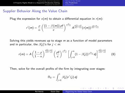
Supplier Behavior Along the Value Chain
Plug the expression for x(m) to obtain a differential equation in r(m):
r ′(m) =ρ
α
((1− β (m)) ρθ
c
) α1−α
Aα(1−ρ)ρ(1−α) (r(m))
ρ−αρ(1−α)
Solving this yields revenues up to stage m as a function of model parametersand in particular, the β(j)’s for j < m:
r(m) = A
(1− ρ1− α
) ρ(1−α)α(1−ρ)
(ρθ
c
) ρ1−ρ
[∫ m
j=0
(1− β(j))α
1−α dj
] ρ(1−α)α(1−ρ)
(8)
Then, solve for the overall profits of the firm by integrating over stages:
ΠS =
∫ 1
j=0
β(j)r ′ (j) dj
Pol Antras Davin Chor Organizing the Global Value Chain
Motivation and IntroductionA Property Rights Model in a Sequential Production Setting
Empirical Evidence
Setup of the ModelKey PredictionsExtensions
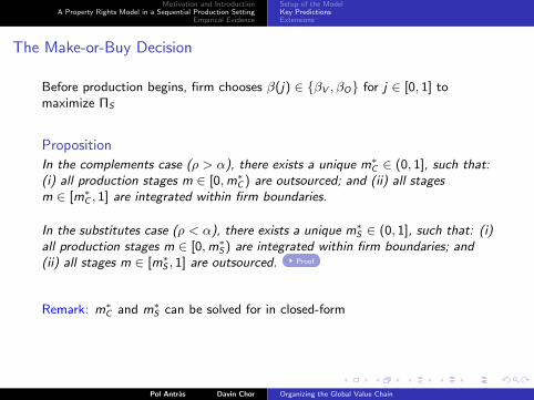
The Make-or-Buy Decision
Before production begins, firm chooses β(j) ∈ βV , βO for j ∈ [0, 1] tomaximize ΠS
Proposition
In the complements case (ρ > α), there exists a unique m∗C ∈ (0, 1], such that:(i) all production stages m ∈ [0,m∗C ) are outsourced; and (ii) all stagesm ∈ [m∗C , 1] are integrated within firm boundaries.
In the substitutes case (ρ < α), there exists a unique m∗S ∈ (0, 1], such that: (i)all production stages m ∈ [0,m∗S) are integrated within firm boundaries; and(ii) all stages m ∈ [m∗S , 1] are outsourced. Proof
Remark: m∗C and m∗S can be solved for in closed-form
Pol Antras Davin Chor Organizing the Global Value Chain

Motivation and IntroductionA Property Rights Model in a Sequential Production Setting
Empirical Evidence
Setup of the ModelKey PredictionsExtensions
The Make-or-Buy Decision (cont.)
Additional predictions:
Proposition
Whenever integration and outsourcing coexist along the value chain, i.e.,m∗C ∈ (0, 1) when ρ > α or m∗S ∈ (0, 1) when ρ < α, a decrease in ρ willnecessarily expand the range of stages that are vertically integrated.
Intuition:
I When ρ is low, firm has high market power, and hence will focus on therent extraction motive for integration
Pol Antras Davin Chor Organizing the Global Value Chain

Motivation and IntroductionA Property Rights Model in a Sequential Production Setting
Empirical Evidence
Setup of the ModelKey PredictionsExtensions
Plan of Talk
1. Motivation and Introduction
2. Setup of the Core Model
3. Key Predictions
4. Extensions
5. Empirical Evidence
6. Conclusion
Pol Antras Davin Chor Organizing the Global Value Chain

Motivation and IntroductionA Property Rights Model in a Sequential Production Setting
Empirical Evidence
Setup of the ModelKey PredictionsExtensions
Extensions
Benchmark model can be readily extended to connect it to the global sourcingframework in Antras and Helpman (2004) by adding:
1. Headquarter intensity
2. Firm heterogeneity
3. Supplier heterogeneity
Extensions are important for helping us to map the theoretical predictions tothe empirics
Pol Antras Davin Chor Organizing the Global Value Chain

Motivation and IntroductionA Property Rights Model in a Sequential Production Setting
Empirical Evidence
Setup of the ModelKey PredictionsExtensions
Summary of Extensions
1. Headquarter intensity: Extension 1
I Introduce Firm investment in headquarter services prior to stage 0; fullynon-contractible
I Obtain: integration more prevalent in headquarter intensive sectors
I Otherwise: Similar to core model, but with ρ replaced by ρ ≡ (1− η)ρ
2. Firm heterogeneity: Extension 2
I θ’s drawn from Pareto distribution; introduce fixed organizational costs
I Converts previous within-firm results into predictions on the relativeprevalence of integration at the industry level
3. Supplier heterogeneity: Extension 3
I Results generalize, but it might be important to control for unobservedcountry cost differences and for selection
Pol Antras Davin Chor Organizing the Global Value Chain

Motivation and IntroductionA Property Rights Model in a Sequential Production Setting
Empirical Evidence
Empirical specificationMeasuring downstreamnessProduction Line Position and the Boundaries of the Firm
Plan of Talk
1. Motivation and Introduction
2. Setup of the Core Model
3. Key Predictions
4. Extensions
5. Empirical Evidence
6. Conclusion
Pol Antras Davin Chor Organizing the Global Value Chain

Motivation and IntroductionA Property Rights Model in a Sequential Production Setting
Empirical Evidence
Empirical specificationMeasuring downstreamnessProduction Line Position and the Boundaries of the Firm
Empirical specification
Sit = β1Di × 1(ρi < ρmed) + β2Di × 1(ρi > ρmed) + β31(ρi > ρmed)
+βX Xi + αt + εit
I Sit : share of intrafirm trade in U.S. imports for industry i , year t
I Data source: U.S. Census Bureau Related Party Database
I 253 manufacturing industries, 11 years (2000-2010)
I Di : “downstreamness” of an industry
I 1(ρi ≷ ρmed): indicator for complements vs substitutes case
I Xi : other industry controls
I αt : year fixed effects (in country-industry-year specifications, includecountry-year fixed effects, αct , instead)
I Cluster standard errors by industry
Pol Antras Davin Chor Organizing the Global Value Chain

Motivation and IntroductionA Property Rights Model in a Sequential Production Setting
Empirical Evidence
Empirical specificationMeasuring downstreamnessProduction Line Position and the Boundaries of the Firm
Measuring downstreamness: Preliminaries
Start with the output identity for industry i in a closed-economy:
Yi = Fi +∑
j
dijYj
= Fi +∑
j
dijFj︸ ︷︷ ︸direct use of i as input
+∑
j
∑k
dikdkjFj +∑
j
∑k
∑l
dildlkdkjFj + . . .
︸ ︷︷ ︸indirect use of i as input
In compact matrix form:
Y = F + DF + D2F + D3F + D4F + . . .
= [I − D]−1 F .
where D is the N × N matrix of direct requirement coefficients; F is the N × 1matrix of final use values (going to consumption and investment)
Pol Antras Davin Chor Organizing the Global Value Chain
Motivation and IntroductionA Property Rights Model in a Sequential Production Setting
Empirical Evidence
Empirical specificationMeasuring downstreamnessProduction Line Position and the Boundaries of the Firm
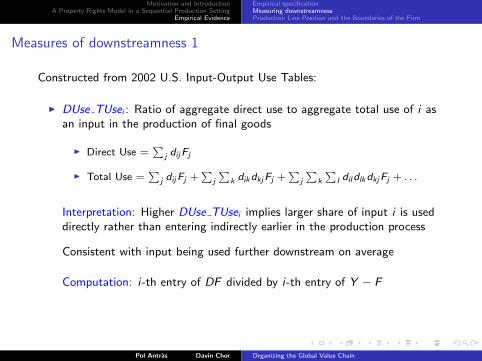
Measures of downstreamness 1
Constructed from 2002 U.S. Input-Output Use Tables:
I DUse TUsei : Ratio of aggregate direct use to aggregate total use of i asan input in the production of final goods
I Direct Use =∑
j dijFj
I Total Use =∑
j dijFj +∑
j
∑k dikdkjFj +
∑j
∑k
∑l dildlkdkjFj + . . .
Interpretation: Higher DUse TUsei implies larger share of input i is useddirectly rather than entering indirectly earlier in the production process
Consistent with input being used further downstream on average
Computation: i-th entry of DF divided by i-th entry of Y − F
Pol Antras Davin Chor Organizing the Global Value Chain

Motivation and IntroductionA Property Rights Model in a Sequential Production Setting
Empirical Evidence
Empirical specificationMeasuring downstreamnessProduction Line Position and the Boundaries of the Firm
Measures of downstreamness 2
I Start with:
Ui = 1 · Fi
Yi+ 2 ·
∑Nj=1 dijFj
Yi+ 3 ·
∑Nj=1
∑Nk=1 dikdkjFj
Yi
+4 ·∑N
j=1
∑Nk=1
∑Nl=1 dildlkdkjFj
Yi+ ...
Interpretation: Take a weighted average distance from final use, where theweights are the industry’s use value at each stage (normalized by Yi )
Computation: i-th entry of [I − D]−2F divided by i-th entry of Y
See Antras, Chor, Fally, and Hillberry (AER P&P 2012) for more
I Ui ≥ 1: Reciprocate to get DownMeasurei , increasing in downstreamness
Pol Antras Davin Chor Organizing the Global Value Chain

Motivation and IntroductionA Property Rights Model in a Sequential Production Setting
Empirical Evidence
Empirical specificationMeasuring downstreamnessProduction Line Position and the Boundaries of the Firm
Measures of downstreamness 2
Remarks:
I ACFH (2012) show that Ui is equivalent to a recursively-defined measureof distance from final use in Fally (2012)
I Also equivalent to a measure of cost-push effects or total “forwardlinkages” in supply-side I-O analysis
Ui is equal to the dollar amount by which output of all sectors increasesfollowing a $1 increase in value-added in sector i
I Empirical implementation: ACFH (2012) show how to apply anopen-economy adjustment to D and F as reported in I-O Tables, toaccount for net exports and net change in inventories
Pol Antras Davin Chor Organizing the Global Value Chain
Motivation and IntroductionA Property Rights Model in a Sequential Production Setting
Empirical Evidence
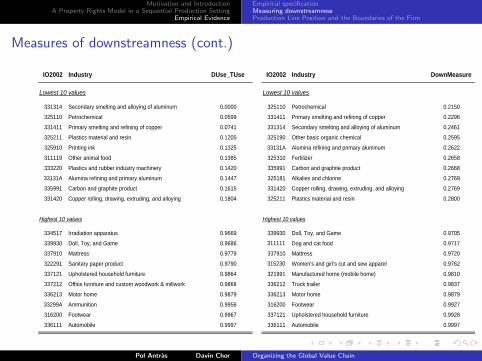
Empirical specificationMeasuring downstreamnessProduction Line Position and the Boundaries of the Firm
Measures of downstreamness (cont.)
IO2002 Industry DUse_TUse IO2002 Industry DownMeasure
331314 Secondary smelting and alloying of aluminum 0.0000 325110 Petrochemical 0.2150
325110 Petrochemical 0.0599 331411 Primary smelting and refining of copper 0.2296
331411 Primary smelting and refining of copper 0.0741 331314 Secondary smelting and alloying of aluminum 0.2461
325211 Plastics material and resin 0.1205 325190 Other basic organic chemical 0.2595
325910 Printing ink 0.1325 33131A Alumina refining and primary aluminum 0.2622
311119 Other animal food 0.1385 325310 Fertilizer 0.2658
333220 Plastics and rubber industry machinery 0.1420 335991 Carbon and graphite product 0.2668
33131A Alumina refining and primary aluminum 0.1447 325181 Alkalies and chlorine 0.2769
335991 Carbon and graphite product 0.1615 331420 Copper rolling, drawing, extruding, and alloying 0.2769
331420 Copper rolling, drawing, extruding, and alloying 0.1804 325211 Plastics material and resin 0.2800
334517 Irradiation apparatus 0.9669 339930 Doll, Toy, and Game 0.9705
339930 Doll, Toy, and Game 0.9686 311111 Dog and cat food 0.9717
337910 Mattress 0.9779 337910 Mattress 0.9720
322291 Sanitary paper product 0.9790 315230 Women's and girl's cut and sew apparel 0.9762
337121 Upholstered household furniture 0.9864 321991 Manufactured home (mobile home) 0.9810
337212 Office furniture and custom woodwork & millwork 0.9868 336212 Truck trailer 0.9837
336213 Motor home 0.9879 336213 Motor home 0.9879
33299A Ammunition 0.9956 316200 Footwear 0.9927
316200 Footwear 0.9967 337121 Upholstered household furniture 0.9928
336111 Automobile 0.9997 336111 Automobile 0.9997
Highest 10 values
Lowest 10 valuesLowest 10 values
Highest 10 values
Pol Antras Davin Chor Organizing the Global Value Chain

Motivation and IntroductionA Property Rights Model in a Sequential Production Setting
Empirical Evidence
Empirical specificationMeasuring downstreamnessProduction Line Position and the Boundaries of the Firm
Measure of ρi
Constructed from Broda and Weinstein’s (2006) estimates of U.S. importdemand elasticities for HS10 products:
I Convert to IO2002 categories using HS-IO concordance
I ρi is the average elasticity taken over all “buying” industries, i.e. industriesthat use i as an input, weighted by the value of input i use in the 2002Input-Output Tables
(Final-use value is included in this calculation; assign it the elasticity ofindustry i itself)
I Baseline specification uses a median value cutoff:
I 1(ρi > ρmed ): complements case
I 1(ρi < ρmed ): substitutes case
Pol Antras Davin Chor Organizing the Global Value Chain

Motivation and IntroductionA Property Rights Model in a Sequential Production Setting
Empirical Evidence
Empirical specificationMeasuring downstreamnessProduction Line Position and the Boundaries of the Firm
Other industry variables
I HQ intensity: log(s/l), log(k/l), log(m/l) from NBER-CESManufacturing Database
I 2000-2005 averages
I Also: consider a breakdown of log(k/l) into log(equipment k/l) andlog(plant k/l), in the spirit of Nunn and Trefler (2008b)
I R&D intensity: log(R&D/Sales) from Orbis, from Nunn and Trefler(2008b)
I Dispersion: log sd of U.S. exports across ports and destinations (Nunn andTrefler 2008a)
I Distinguish between industry variables constructed for the:
I input “selling” industry
I input “buying” industry (more consistent with our model)
Pol Antras Davin Chor Organizing the Global Value Chain
Motivation and IntroductionA Property Rights Model in a Sequential Production Setting
Empirical Evidence
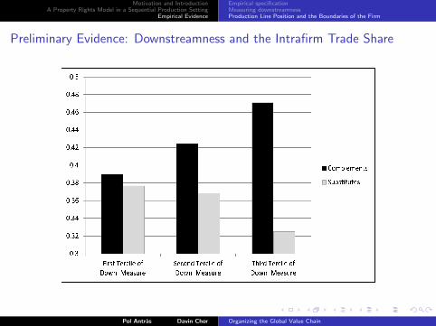
Empirical specificationMeasuring downstreamnessProduction Line Position and the Boundaries of the Firm
Preliminary Evidence: Downstreamness and the Intrafirm Trade Share
Pol Antras Davin Chor Organizing the Global Value Chain

Motivation and IntroductionA Property Rights Model in a Sequential Production Setting
Empirical Evidence
Empirical specificationMeasuring downstreamnessProduction Line Position and the Boundaries of the Firm
Evidence: DUse TUsei
I Greater propensity to integrate downstream in complements case; to outsourcedownstream in substitutes case
(1) (2) (3) (4) (5) (6) (7) (8)Elas < Median Elas >= Median Weighted Weighted
Log (s/l) 0.005 0.039 0.056 0.112* 0.038 -0.098 0.005 -0.068[0.044] [0.043] [0.042] [0.064] [0.055] [0.079] [0.020] [0.076]
Log (k/l) 0.044 0.034[0.029] [0.027]
Log (equipment k / l) 0.085** 0.022 0.153*** 0.188*** 0.026 0.134***[0.034] [0.047] [0.043] [0.061] [0.016] [0.051]
Log (plant k / l) -0.077* -0.011 -0.159** -0.151** -0.056*** -0.142***[0.045] [0.057] [0.064] [0.070] [0.019] [0.050]
Log (materials/l) 0.058* 0.060* 0.065* 0.049 0.072 0.060 0.025* 0.080[0.035] [0.034] [0.033] [0.049] [0.047] [0.058] [0.014] [0.049]
Log (0.001+ R&D/Sales) 0.055*** 0.054*** 0.053*** 0.050*** 0.054*** 0.090*** 0.031*** 0.073***[0.009] [0.009] [0.009] [0.013] [0.013] [0.018] [0.004] [0.016]
Dispersion 0.081 0.061 0.103 0.034 0.188* 0.160 0.108*** 0.083[0.070] [0.070] [0.075] [0.108] [0.100] [0.124] [0.038] [0.108]
DUse_TUse -0.018 -0.216*** 0.225***[0.054] [0.075] [0.069]
DUse_TUse X 1(Elas < Median) -0.196*** -0.174** -0.166* -0.115*** -0.075[0.071] [0.072] [0.089] [0.033] [0.073]
DUse_TUse X 1(Elas > Median) 0.171** 0.198*** 0.482*** -0.035 0.352***[0.067] [0.068] [0.123] [0.030] [0.118]
1(Elas > Median) -0.191*** -0.191*** -0.410*** -0.049* -0.291***[0.062] [0.061] [0.085] [0.029] [0.075]
Industry controls for: Buyer Buyer Buyer Buyer Buyer Buyer Buyer BuyerYear fixed effects? Yes Yes Yes Yes Yes Yes No NoCountry-Year fixed effects? No No No No No No Yes Yes
Observations 2783 2783 2783 1375 1408 2783 207991 207991R-squared 0.27 0.32 0.33 0.37 0.28 0.61 0.18 0.59
Pol Antras Davin Chor Organizing the Global Value Chain

Motivation and IntroductionA Property Rights Model in a Sequential Production Setting
Empirical Evidence
Empirical specificationMeasuring downstreamnessProduction Line Position and the Boundaries of the Firm
Evidence: DownMeasurei
I Similarly strong evidence particularly for the complements case
(1) (2) (3) (4) (5) (6) (7) (8)Elas < Median Elas >= Median Weighted Weighted
Log (s/l) -0.011 0.019 0.037 0.088 0.032 -0.143** 0.000 -0.097*[0.045] [0.042] [0.041] [0.067] [0.051] [0.058] [0.020] [0.054]
Log (k/l) 0.062** 0.058**[0.027] [0.026]
Log (equipment k / l) 0.125*** 0.061 0.192*** 0.157** 0.039** 0.139***[0.036] [0.047] [0.048] [0.066] [0.017] [0.047]
Log (plant k / l) -0.100** -0.027 -0.192*** -0.091 -0.062*** -0.117**[0.049] [0.061] [0.073] [0.080] [0.020] [0.052]
Log (materials/l) 0.050 0.043 0.049 0.022 0.064 0.032 0.017 0.046[0.033] [0.033] [0.032] [0.050] [0.043] [0.055] [0.014] [0.043]
Log (0.001+ R&D/Sales) 0.058*** 0.054*** 0.054*** 0.053*** 0.050*** 0.089*** 0.032*** 0.072***[0.010] [0.009] [0.009] [0.014] [0.014] [0.017] [0.004] [0.014]
Dispersion 0.087 0.092 0.150* 0.082 0.258** 0.249* 0.116*** 0.163[0.072] [0.076] [0.079] [0.114] [0.105] [0.147] [0.043] [0.114]
DownMeasure 0.101* -0.036 0.342***[0.055] [0.069] [0.081]
DownMeasure X 1(Elas < Median) -0.024 0.025 -0.119 -0.002 -0.002[0.064] [0.065] [0.107] [0.035] [0.091]
DownMeasure X 1(Elas > Median) 0.249*** 0.298*** 0.526*** -0.039 0.440***[0.085] [0.081] [0.100] [0.033] [0.089]
1(Elas > Median) -0.115* -0.110* -0.386*** 0.022 -0.279***[0.064] [0.062] [0.081] [0.030] [0.072]
Industry controls for: Buyer Buyer Buyer Buyer Buyer Buyer Buyer BuyerYear fixed effects? Yes Yes Yes Yes Yes Yes No NoCountry-Year fixed effects? No No No No No No Yes Yes
Observations 2783 2783 2783 1375 1408 2783 207991 207991R-squared 0.28 0.31 0.33 0.33 0.33 0.64 0.18 0.61
Pol Antras Davin Chor Organizing the Global Value Chain

Motivation and IntroductionA Property Rights Model in a Sequential Production Setting
Empirical Evidence
Empirical specificationMeasuring downstreamnessProduction Line Position and the Boundaries of the Firm
Evidence: Production Line Position and the Boundaries of the Firm
I Results evident with a more flexible quintile treatment of ρi
(1) (2) (3) (4) (5) (6)
Downstreamness: DUse_TUse DUse_TUse DUse_TUse DownMeasure DownMeasure DownMeasure
Weighted Weighted Weighted Weighted
Downstream X 1(Elas Quintile 1) -0.165* -0.252* -0.138 0.049 -0.283 -0.089[0.093] [0.148] [0.100] [0.119] [0.202] [0.142]
Downstream X 1(Elas Quintile 2) -0.173 -0.100 -0.037 -0.042 -0.154 -0.040[0.108] [0.136] [0.115] [0.099] [0.139] [0.122]
Downstream X 1(Elas Quintile 3) -0.145 0.008 0.051 0.019 0.114 0.224[0.130] [0.166] [0.153] [0.124] [0.166] [0.172]
Downstream X 1(Elas Quintile 4) 0.215** 0.159 0.066 0.332*** 0.066 0.073[0.100] [0.142] [0.119] [0.126] [0.174] [0.120]
Downstream X 1(Elas Quintile 5) 0.198* 0.781*** 0.637*** 0.312** 0.736*** 0.621***[0.103] [0.194] [0.199] [0.130] [0.110] [0.096]
Industry controls for: Buyer Buyer Buyer Buyer Buyer BuyerElas Quintile dummies? Yes Yes Yes Yes Yes YesYear fixed effects Yes Yes No Yes Yes NoCountry-Year fixed effects No No Yes No No Yes
Observations 2783 2783 207991 2783 2783 207991R-squared 0.34 0.64 0.61 0.34 0.67 0.62
Pol Antras Davin Chor Organizing the Global Value Chain

Motivation and IntroductionA Property Rights Model in a Sequential Production Setting
Empirical Evidence
Empirical specificationMeasuring downstreamnessProduction Line Position and the Boundaries of the Firm
Robustness Tests
I Robust to controlling for: (i) value-added share; (ii) input “importance”; (iii)contractibility (Nunn and Trefler 2008); (iv) intermediation (Bernard et al. 2010)
(1) (2) (3) (4) (5)
DUse_TUse X 1(Elas < Median) -0.187** -0.177** -0.103 -0.180** -0.130*[0.074] [0.072] [0.071] [0.077] [0.079]
DUse_TUse X 1(Elas > Median) 0.157** 0.198*** 0.236*** 0.159** 0.158**[0.077] [0.068] [0.065] [0.068] [0.074]
Value-added / Value shipments 0.187 0.216*[0.135] [0.125]
Input "Importance" -1.687 -1.453[1.231] [1.302]
Intermediation -0.464*** -0.413***[0.106] [0.102]
Own Contractibility 0.019 0.024[0.048] [0.047]
Buyer contractibility -0.199*** -0.169**[0.067] [0.065]
Year fixed effects? Yes Yes Yes Yes Yes
Observations 2783 2783 2783 2783 2783R-squared 0.33 0.33 0.38 0.37 0.41
Pol Antras Davin Chor Organizing the Global Value Chain

Motivation and IntroductionA Property Rights Model in a Sequential Production Setting
Empirical Evidence
Empirical specificationMeasuring downstreamnessProduction Line Position and the Boundaries of the Firm
Extension 1: Headquarter Intensity
Theory predicts that:
I In complements case, ρ(1− η) high, greater propensity to integratedownstream when ρ is high and η is low
I In substitutes case, ρ(1− η) low, greater propensity to outsourcedownstream when ρ is low and η is high
I Suggests a triple interaction approach: further interaction with hq intensity
Use first principal component of log(s/l), log(equipment k/l), andlog(R&D/Sales) as measure of headquarter intensity.
I Complements case: results indeed strongest in lowest quintile of η
I Substitutes case: results more noisy but broadly supportive
Pol Antras Davin Chor Organizing the Global Value Chain

Motivation and IntroductionA Property Rights Model in a Sequential Production Setting
Empirical Evidence
Empirical specificationMeasuring downstreamnessProduction Line Position and the Boundaries of the Firm
Extension 1: Headquarter Intensity (cont.)(1) (2) (3) (4) (5) (6)
Downstreamness: DUse_TUse DUse_TUse DUse_TUse DownMeasure DownMeasure DownMeasure
Buyer industry hq intensity:
Weighted Weighted Weighted Weighted
Downstream X 1 (Elas < Med) X (HQ Quintile 1) 0.049 0.009 -0.016 0.351*** 0.301** 0.290**[0.129] [0.139] [0.118] [0.128] [0.134] [0.129]
Downstream X 1 (Elas < Med) X (HQ Quintile 2) -0.268** -0.477*** -0.331** -0.161 -0.312* -0.169[0.118] [0.162] [0.148] [0.103] [0.186] [0.150]
Downstream X 1 (Elas < Med) X (HQ Quintile 3) -0.175 -0.162 -0.158 0.072 -0.02 -0.058[0.148] [0.138] [0.124] [0.131] [0.160] [0.145]
Downstream X 1 (Elas < Med) X (HQ Quintile 4) -0.377*** -0.658*** -0.455*** -0.121 -0.394** -0.280**[0.134] [0.108] [0.069] [0.128] [0.172] [0.125]
Downstream X 1 (Elas < Med) X (HQ Quintile 5) 0.177 -0.046 0.024 0.229 -0.181 -0.05[0.171] [0.192] [0.172] [0.157] [0.160] [0.158]
Downstream X 1 (Elas > Med) X (HQ Quintile 1) 0.196 0.805** 0.798*** 0.465*** 0.624*** 0.593***[0.248] [0.325] [0.278] [0.163] [0.113] [0.087]
Downstream X 1 (Elas > Med) X (HQ Quintile 2) -0.037 -0.099 -0.180 0.032 -0.001 -0.061[0.146] [0.181] [0.175] [0.130] [0.238] [0.189]
Downstream X 1 (Elas > Med) X (HQ Quintile 3) 0.216* 0.172 0.027 0.358*** 0.357 0.099[0.119] [0.207] [0.145] [0.135] [0.257] [0.199]
Downstream X 1 (Elas > Med) X (HQ Quintile 4) 0.130 0.819** 0.427 0.280* 0.519 0.079[0.161] [0.390] [0.341] [0.159] [0.427] [0.352]
Downstream X 1 (Elas > Med) X (HQ Quintile 5) 0.183** 0.271* 0.162 0.179 0.274 0.225*[0.082] [0.144] [0.114] [0.117] [0.197] [0.117]
Industry controls for: Buyer Buyer Buyer Buyer Buyer BuyerMain and double interaction effects? Yes Yes Yes Yes Yes YesYear fixed effects? Yes Yes No Yes Yes NoCountry-Year fixed effects? No No Yes No No Yes
Observations 2783 2783 207991 2783 2783 207991R-squared 0.40 0.69 0.63 0.40 0.71 0.65
First Principal Component: Log (s/l), Log (equipment k/l), and Log (0.001+R&D/Sales)
Pol Antras Davin Chor Organizing the Global Value Chain

Motivation and IntroductionA Property Rights Model in a Sequential Production Setting
Empirical Evidence
Empirical specificationMeasuring downstreamnessProduction Line Position and the Boundaries of the Firm
Extension 2: Firm HeterogeneityI Highest propensity to integrate in the first quintile of downstreamness whenρ < ρmed ; and in the last quintile of downstreamness when ρ > ρmed
(1) (2) (3) (4) (5) (6)
Downstreamness: DUse_TUse DUse_TUse DUse_TUse DownMeasure DownMeasure DownMeasure
Weighted Weighted Weighted Weighted
(Downstream Quin 1) X 1(Elas < Median) 0.101** 0.210*** 0.145*** 0.060 0.184*** 0.145**[0.045] [0.058] [0.045] [0.051] [0.067] [0.059]
(Downstream Quin 2) X 1(Elas < Median) 0.041 0.131** 0.096* -0.005 0.062 0.019[0.043] [0.062] [0.054] [0.045] [0.069] [0.055]
(Downstream Quin 3) X 1(Elas < Median) 0.008 0.063 0.010 -0.016 0.089 0.049[0.046] [0.057] [0.046] [0.049] [0.076] [0.060]
(Downstream Quin 4) X 1(Elas < Median) -0.047 0.092 0.047 0.024 0.064 0.032[0.043] [0.065] [0.051] [0.045] [0.075] [0.058]
(Downstream Quin 5) X 1(Elas < Median) 0.017 0.084 0.082 0.023 0.039 0.058[0.042] [0.063] [0.053] [0.042] [0.081] [0.064]
(Downstream Quin 2) X 1(Elas > Median) 0.021 0.031 0.016 0.013 -0.054 -0.068[0.036] [0.067] [0.056] [0.039] [0.069] [0.052]
(Downstream Quin 3) X 1(Elas > Median) 0.086** 0.150** 0.072 0.035 0.076 0.018[0.044] [0.065] [0.052] [0.047] [0.069] [0.066]
(Downstream Quin 4) X 1(Elas > Median) 0.030 0.086 0.017 0.073* 0.056 0.013[0.048] [0.056] [0.050] [0.043] [0.072] [0.060]
(Downstream Quin 5) X 1(Elas > Median) 0.181*** 0.352*** 0.257*** 0.171*** 0.380*** 0.300***[0.048] [0.067] [0.062] [0.059] [0.085] [0.074]
Industry controls for: Buyer Buyer Buyer Buyer Buyer BuyerDownstream quin and Elasticity dummies? Yes Yes Yes Yes Yes YesYear fixed effects Yes Yes No Yes Yes NoCountry-Year fixed effects No No Yes No No Yes
Observations 2783 2783 207991 2783 2783 207991R-squared 0.35 0.63 0.61 0.33 0.67 0.63
Dependent variable: Intrafirm Import Share
Pol Antras Davin Chor Organizing the Global Value Chain

Motivation and IntroductionA Property Rights Model in a Sequential Production Setting
Empirical Evidence
Empirical specificationMeasuring downstreamnessProduction Line Position and the Boundaries of the Firm
Selection into intrafirm trade (Heckman selection)
I Excluded variable in the second-stage: interaction of measure of country costs ofentry and R&D intensity of the selling industry
(1) (2) (3) (4) (5) (6)
Downstreamness: DUse_TUse DUse_TUse DUse_TUse DownMeasure DownMeasure DownMeasure
Probit Weighted Weighted Probit Weighted Weighted
Downstream X 1(Elas < Median) 0.047 -0.073 -0.072 0.634** -0.020 -0.011[0.310] [0.074] [0.074] [0.317] [0.097] [0.088]
Downstream X 1(Elas > Median) 0.274 0.310*** 0.314*** -0.291 0.353*** 0.347***[0.252] [0.106] [0.102] [0.246] [0.078] [0.084]
1(Elas > Median) 0.003 -0.268*** -0.268*** 0.661*** -0.244*** -0.234***[0.231] [0.075] [0.075] [0.233] [0.076] [0.073]
Seller Log (0.001+ R&D/Sales) -0.028*** -0.028*** X Country Entry Costs [0.007] [0.007]Seller Log (0.001+ R&D/Sales) 0.030 0.026
[0.045] [0.041]Inverse Mills Ratio -0.120 -0.082
[0.250] [0.197]
Industry controls for: Buyer Buyer Buyer Buyer Buyer BuyerCountry-year fixed effects? Yes Yes Yes Yes Yes Yes
Sample: Total imports >=0
Total imports > 0
Total imports > 0
Total imports >=0
Total imports > 0
Total imports > 0
Observations 462990 186029 186029 462990 186029 186029R-squared - 0.63 0.63 - 0.64 0.64
Pol Antras Davin Chor Organizing the Global Value Chain

Motivation and IntroductionA Property Rights Model in a Sequential Production Setting
Empirical Evidence
Empirical specificationMeasuring downstreamnessProduction Line Position and the Boundaries of the Firm
Plan of Talk
1. Motivation and Introduction
2. Setup of the Core Model
3. Key Predictions
4. Extensions
5. Empirical Evidence
6. Conclusion
Pol Antras Davin Chor Organizing the Global Value Chain
Motivation and IntroductionA Property Rights Model in a Sequential Production Setting
Empirical Evidence
Empirical specificationMeasuring downstreamnessProduction Line Position and the Boundaries of the Firm
Concluding Remarks
I Developed a model of organizational decisions for a production functionwith a continuum of sequential stages
I For each stage, firm’s make-or-buy decision depends on that stage’sposition in the value chain
I When stage inputs are sequential complements: Outsource upstream andIntegrate downstream
I When stage inputs are sequential substitutes: Integrate upstream andOutsource downstream
I Intuition driven by how effort choices of upstream stage suppliers affecteffort levels downstream
I Can be readily embedded into existing global sourcing frameworks
I Evidence based on U.S. related-party trade shares is broadly consistentwith the model’s predictions
Pol Antras Davin Chor Organizing the Global Value Chain

Motivation and IntroductionA Property Rights Model in a Sequential Production Setting
Empirical Evidence
Empirical specificationMeasuring downstreamnessProduction Line Position and the Boundaries of the Firm
The Make-or-Buy Decision
Proof heuristic:
For a given stage m, adopt the solution approach in Antras and Helpman(2004, 2008) and consider the hypothetical case in which β(m) can be chosenfrom the continuum of values in [0, 1]
Let β∗(m) denote the unconstrained bargaining share that solves ∂ΠS∂β(m)
= 0
Consider the behavior of β∗(m) in the two cases
Return
Pol Antras Davin Chor Organizing the Global Value Chain
Motivation and IntroductionA Property Rights Model in a Sequential Production Setting
Empirical Evidence
Empirical specificationMeasuring downstreamnessProduction Line Position and the Boundaries of the Firm
The Make-or-Buy Decision: Sequential Complements
For ρ > α: Tend to choose βO upstream, βV downstream
m
β(m)
1
1
Locus: Φ = 0 (ρ > α case)
0
1− α
Pol Antras Davin Chor Organizing the Global Value Chain
Motivation and IntroductionA Property Rights Model in a Sequential Production Setting
Empirical Evidence
Empirical specificationMeasuring downstreamnessProduction Line Position and the Boundaries of the Firm
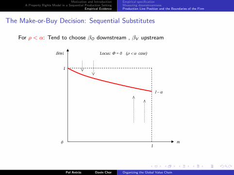
The Make-or-Buy Decision: Sequential Substitutes
For ρ < α: Tend to choose βO downstream , βV upstream
m
β(m)
1
1
Locus: Φ = 0 (ρ < α case)
0
1− α
Pol Antras Davin Chor Organizing the Global Value Chain

Motivation and IntroductionA Property Rights Model in a Sequential Production Setting
Empirical Evidence
Empirical specificationMeasuring downstreamnessProduction Line Position and the Boundaries of the Firm
Extension 1: Headquarter Intensity
q = θ
(h
η
)η (∫ 1
0
(x(j)
1− η
)αI (j)dj
) 1−ηα
(9)
I Headquarter services, h, are fully noncontractible
I Provided by the firm before stage 0 commences
I All stage suppliers take h as given when they decide on x(j)
I η ∈ (0, 1): intensity of headquarter services
Return
Pol Antras Davin Chor Organizing the Global Value Chain

Motivation and IntroductionA Property Rights Model in a Sequential Production Setting
Empirical Evidence
Empirical specificationMeasuring downstreamnessProduction Line Position and the Boundaries of the Firm
Extension 1: Headquarter Intensity (cont.)
I With the same demand function as before, this yields:
r(m) = A1−ρθρ(
h
η
)ρη(1− η)−ρ
[∫ m
0
x(j)αdj
] ρα
I This turns out to behave like the core model, but with ρ replaced byρ ≡ (1− η)ρ
Proposition
In the presence of headquarter services provided by the firm, the results inPropositions 1 and 2 continue to hold except for the fact that: (i) thecomplements and substitutes cases are now defined by ρ ≡ (1− η) ρ > α andρ ≡ (1− η) ρ < α, respectively, and (ii) the range of stages that are verticallyintegrated is now also (weakly) increasing in η.
Pol Antras Davin Chor Organizing the Global Value Chain

Motivation and IntroductionA Property Rights Model in a Sequential Production Setting
Empirical Evidence
Empirical specificationMeasuring downstreamnessProduction Line Position and the Boundaries of the Firm
Extension 1: Headquarter Intensity (cont.)
Remarks:
I Part (ii) of the proposition implies that the propensity to integrate rises ashq services become more important in production (η rises)
I Recovers the Antras (2003) result, although the empirical implementationwill call for a slight variation:
If we interpret hq services as being capital- or R&D-intensive, then wouldexpect the share of intrafirm trade for a given input to be increasing in the(average) capital or R&D intensity of industries that buy the input inquestion
I Also from part (i) of the proposition, note that the likelihood that we findourselves in the sequential complements case is lower the higher isheadquarter intensity
I This is an auxiliary prediction of the model that we will test
Pol Antras Davin Chor Organizing the Global Value Chain
Motivation and IntroductionA Property Rights Model in a Sequential Production Setting
Empirical Evidence
Empirical specificationMeasuring downstreamnessProduction Line Position and the Boundaries of the Firm
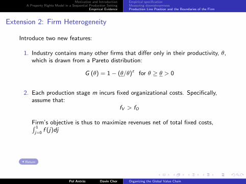
Extension 2: Firm Heterogeneity
Introduce two new features:
1. Industry contains many other firms that differ only in their productivity, θ,which is drawn from a Pareto distribution:
G (θ) = 1− (θ/θ)z for θ ≥ θ > 0
2. Each production stage m incurs fixed organizational costs. Specifically,assume that:
fV > fO
Firm’s objective is thus to maximize revenues net of total fixed costs,∫ 1
j=0f (j)dj
Return
Pol Antras Davin Chor Organizing the Global Value Chain

Motivation and IntroductionA Property Rights Model in a Sequential Production Setting
Empirical Evidence
Empirical specificationMeasuring downstreamnessProduction Line Position and the Boundaries of the Firm
Extension 2: Firm Heterogeneity (cont.)
m
1
0
mC*
C
mC
Complements Case
m
1
mS*
mS
S
Substitutes Case
Firms integrating stage mC
Firms outsourcing stage mC
Firms integrating stage mS
Firms outsourcing stage mS
Complements case (ρ > α):
I For each θ, there exists a cutoff stage mC (θ) such that all stages beforemC (θ) are outsourced, and all stages after are integrated
I mC (θ) is decreasing in θ
Pol Antras Davin Chor Organizing the Global Value Chain

Motivation and IntroductionA Property Rights Model in a Sequential Production Setting
Empirical Evidence
Empirical specificationMeasuring downstreamnessProduction Line Position and the Boundaries of the Firm
Extension 2: Firm Heterogeneity (cont.)
m
1
0
mC*
C
mC
Complements Case
m
1
mS*
mS
S
Substitutes Case
Firms integrating stage mC
Firms outsourcing stage mC
Firms integrating stage mS
Firms outsourcing stage mS
Conversely, in the substitutes case (ρ < α):
I For each θ, there exists a cutoff stage mS(θ) such that all stages beforemS(θ) are integrated, and all stages after are outsourced
I mS(θ) is increasing in θ
Pol Antras Davin Chor Organizing the Global Value Chain

Motivation and IntroductionA Property Rights Model in a Sequential Production Setting
Empirical Evidence
Empirical specificationMeasuring downstreamnessProduction Line Position and the Boundaries of the Firm
Extension 2: Firm Heterogeneity (cont.)
Importantly, this generates smooth predictions for how the intrafirm trade sharevaries with production line position:
Proposition
The share of firms integrating a particular stage m is weakly increasing in thedownstreamness of that stage in the complements case (ρ > α), while it isdecreasing in the downstreamness of the stage in the substitutes case (ρ < α).
Furthermore, the share of firms integrating a particular stage m, is weaklyincreasing in the dispersion of productivity within the industry.
I This converts previous within-firm variation on the propensity to integratedifferent stages into predictions regarding the relative prevalence ofintegration of an input with a particular level of downstreamness
I If fixed costs of integration are relatively high, only most downstream (incomplements case) or most upstream stages (in substitutes case) will beintegrated
Pol Antras Davin Chor Organizing the Global Value Chain

Motivation and IntroductionA Property Rights Model in a Sequential Production Setting
Empirical Evidence
Empirical specificationMeasuring downstreamnessProduction Line Position and the Boundaries of the Firm
Extension 3: Input and Supplier Heterogeneity
Relaxing the symmetry in the production function:
q = θ
(∫ 1
0
(ψ (j) x(j))α I (j)dj
)1/α
(10)
In practice:
I Production stages can have different weights
I Stage suppliers could defer in their productivity levels
Separately, production costs for stage j , c(j), might depend on which countrythe stage is located in
Return
Pol Antras Davin Chor Organizing the Global Value Chain

Motivation and IntroductionA Property Rights Model in a Sequential Production Setting
Empirical Evidence
Empirical specificationMeasuring downstreamnessProduction Line Position and the Boundaries of the Firm
Extension 3: Input and Supplier Heterogeneity (cont.)
This more general model can be solved using a similar heuristic:
Proposition
Suppose that technology allows for input heterogeneity as in (10) and thatmarginal costs of production of inputs are also heterogeneous and given by c (j)for j ∈ [0, 1].
Then the share of firms integrating a particular stage m is weakly increasing inthe downstreamness of that stage in the complements case (ρ > α), while it isdecreasing in the downstreamness of that stage in the substitutes case (ρ < α).
Pol Antras Davin Chor Organizing the Global Value Chain
Motivation and IntroductionA Property Rights Model in a Sequential Production Setting
Empirical Evidence
Empirical specificationMeasuring downstreamnessProduction Line Position and the Boundaries of the Firm
Extension 3: Input and Supplier Heterogeneity (cont.)
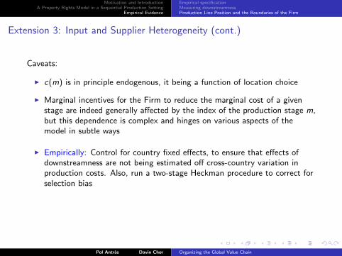
Caveats:
I c(m) is in principle endogenous, it being a function of location choice
I Marginal incentives for the Firm to reduce the marginal cost of a givenstage are indeed generally affected by the index of the production stage m,but this dependence is complex and hinges on various aspects of themodel in subtle ways
I Empirically: Control for country fixed effects, to ensure that effects ofdownstreamness are not being estimated off cross-country variation inproduction costs. Also, run a two-stage Heckman procedure to correct forselection bias
Pol Antras Davin Chor Organizing the Global Value Chain