Embed Size (px)
Citation preview

NREL is a national laboratory of the U.S. Department of Energy Office of Energy Efficiency & Renewable Energy Operated by the Alliance for Sustainable Energy, LLC This report is available at no cost from the National Renewable Energy Laboratory (NREL) at www.nrel.gov/publications.
Contract No. DE-AC36-08GO28308
Technical Report NREL/TP-5000-74597 October 2019
Oregon Offshore Wind Site Feasibility and Cost Study Walter Musial,1 Philipp Beiter,1 Jake Nunemaker,1 Donna Heimiller,1 Josh Ahmann,2 and Jason Busch3
1 National Renewable Energy Laboratory 2 Parametrix 3 Pacific Ocean Energy Trust
NREL is a national laboratory of the U.S. Department of Energy Office of Energy Efficiency & Renewable Energy Operated by the Alliance for Sustainable Energy, LLC This report is available at no cost from the National Renewable Energy Laboratory (NREL) at www.nrel.gov/publications.
Contract No. DE-AC36-08GO28308
National Renewable Energy Laboratory 15013 Denver West Parkway Golden, CO 80401 303-275-3000 • www.nrel.gov
Technical Report NREL/TP-5000-74597 October 2019
Oregon Offshore Wind Site Feasibility and Cost Study Walter Musial,1 Philipp Beiter,1 Jake Nunemaker,1 Donna Heimiller,1 Josh Ahmann,2 and Jason Busch3
1 National Renewable Energy Laboratory 2 Parametrix 3 Pacific Ocean Energy Trust This report is available from the Bureau of Ocean Energy Management by referencing OCS Study BOEM 2019-046.
Suggested Citation Musial, Walter, Philipp Beiter, Jake Nunemaker, Donna Heimiller, Josh Ahmann, and Jason Busch. 2019. Oregon Offshore Wind Site Feasibility and Cost Study. NREL/TP-5000-74597. nrel.gov/docs/fy20osti/74597.pdf.

NOTICE
This work was authored in part by the National Renewable Energy Laboratory, operated by Alliance for Sustainable Energy, LLC, for the U.S. Department of Energy (DOE) under Contract No. DE-AC36-08GO28308. Funding provided by the U.S. Department of the Interior, Bureau of Ocean Energy Management. The views expressed herein do not necessarily represent the views of the DOE or the U.S. Government.
This report is available at no cost from the National Renewable Energy Laboratory (NREL) at www.nrel.gov/publications.
U.S. Department of Energy (DOE) reports produced after 1991 and a growing number of pre-1991 documents are available free via www.OSTI.gov.
Cover Photos by Dennis Schroeder: (clockwise, left to right) NREL 51934, NREL 45897, NREL 42160, NREL 45891, NREL 48097, NREL 46526.
NREL prints on paper that contains recycled content.

iii
This report is available at no cost from the National Renewable Energy Laboratory at www.nrel.gov/publications.
Acknowledgments This study was funded by the U.S. Department of the Interior, Bureau of Ocean Energy Management Pacific Region, through interagency agreement number M14PG00038 modification 007 with the U.S. Department of Energy National Renewable Energy Laboratory (NREL). The authors would like to thank the many people who contributed to the content of this report including the Bureau of Ocean Energy Management staff: Sara Guiltinan, Necy Sumait, Doug Boren, Joan Barminski, and Whitney Hauer, as well as other bureau team members for their thoughtful reviews, comments, and suggestions.
We also want to thank the NREL contributors including Tiffany Byrne, who coordinated the project schedule and deliverables at NREL, and Donna Heimiller, Caroline Draxl, and Mike Optis, for their contributions to the content of the maps, analysis, and expert consultation in writing this report. Technical editing was provided by Sheri Anstedt. Any errors or omissions are the sole responsibility of the authors.
Principle Power, Inc. was instrumental in supporting the cost analysis for this study and cooperating with NREL to assess the cost impact of project size. Specifically, the authors would like to thank Aaron Smith, Kevin Banister, and Loris Canizares for their individual contributions.
In addition, the authors would especially like to recognize the technical advisory committee for this project, which was led by Jason Busch of the Pacific Ocean Energy Trust. These advisors also provided extensive support in the peer review of this document. The advisory committee members include:
• Jason Busch–Pacific Ocean Energy Trust (committee chair) • Adam Schultz–Oregon Department of Energy • Andy Lanier–Department of Land Conservation and Development • Bryson Robertson–Pacific Marine Energy Center, Oregon State University • Crystal Ball–Bonneville Power Administration • John Schaad–Bonneville Power Administration • Jimmy Lindsay–Portland General Electric • Mike Starrett–Northwest Power and Conservation Council • Rebecca O'Neil–Pacific Northwest National Laboratory.
In particular, the contributions of John Schaad with the Bonneville Power Administration and Mike Starrett of the Northwest Power and Conservation Council were invaluable in helping us connect the wind resources with the power use patterns of the Oregon region.

iv
This report is available at no cost from the National Renewable Energy Laboratory at www.nrel.gov/publications.
List of Acronyms AEP annual energy production BOEM Bureau of Ocean Energy Management BPA Bonneville Power Administration CapEx capital expenditures COD commercial operation date DC direct current DOE U.S. Department of Energy DTU Technical University of Denmark FCR fixed charge rate GIS geographic information system GW gigawatt GWh gigawatt-hour km kilometer kW kilowatt kWh kilowatt-hour LCOE levelized cost of energy m meter MW megawatt MWh megawatt-hour nm nautical miles NCF net capacity factor NOAA National Oceanic and Atmospheric Administration NREL National Renewable Energy Laboratory OCS Outer Continental Shelf O&M operation and maintenance OpEx operational expenditures ORCA Offshore Regional Cost Analyzer POET Pacific Ocean Energy Trust TWh terawatt-hour

v
This report is available at no cost from the National Renewable Energy Laboratory at www.nrel.gov/publications.
Executive Summary To accomplish any significant deployment in the Pacific region, and specifically in Oregon, floating wind energy technologies will be required. These technologies are needed because 97% of the 62 gigawatts of available technical offshore wind energy resource in Oregon is in water depths greater than 60 meters (m). Although floating offshore wind energy technology is still in a nascent stage of development, it is advancing toward commercialization in both Europe and Asia.1
The objectives of this study are to:
• Provide the Bureau of Ocean Energy Management (BOEM) and the state of Oregon with cost data based on geospatial site-specific data to allow for consideration of floating offshore wind in the state’s future energy portfolio
• Inform Oregon’s long-term energy planning activities, which could determine how offshore wind might contribute to future energy supplies.
In this study, we draw from the following data sources:
• Proprietary industry data on floating component costs and pilot-scale costs • Commercial auction price points and costs from fixed-bottom offshore wind projects • Published literature and press information • Oregon geospatial data from resource and regulatory management agencies • Semi-structured interviews with subject matter experts • Cost modeling tools at the National Renewable Energy Laboratory (NREL) • Other offshore wind industry data sources (e.g., Hundleby et al. 2017) • Geographical and wind resource databases such as NREL’s Wind Integration National
Dataset (WIND) Toolkit, which includes mesoscale meteorological data covering much of North America
• Utility-supplied (Bonneville Power Administration [BPA]) transmission and energy use information
• Previous studies performed by NREL for BOEM (e.g., Musial et al. 2016a).
The work performed in the study focused on assessing the present and future costs of floating offshore wind technology deployment in the state of Oregon at commercial scale. The study was performed by NREL and its subcontractors and was funded by BOEM. The study builds off a previous report published by NREL in December 2016, titled “Potential Offshore Wind Energy Areas in California: An Assessment of Locations, Technology, and Costs” (Musial et al. 2016a) also funded by BOEMwhich estimated LCOE for floating offshore wind in California at $100/megawatt-hour (MWh)2 or less by the year 2030.
Since 2016, when the California cost study was conducted, the technologies for both fixed-bottom and floating offshore wind have progressed at a rapid rate, technologically and
1 The first multiturbine commercial floating wind project was commissioned in Scotland in 2017 by Equinor. 2 All cost estimates in this report are denoted in $2018, unless indicated otherwise.

vi
This report is available at no cost from the National Renewable Energy Laboratory at www.nrel.gov/publications.
economically. Based on this progress, several new elements that were not available for the California study are included in this Oregon study. Some of these new considerations include:
• Recent European strike price data, which show a decline of about 65%, relative to 2017, for projects expected to be commissioned by 2025 (Beiter et al. 2017)
• New U.S. price data as well as analysis of the executed Vineyard Wind power purchase agreement, a planned fixed-bottom project in Massachusetts (Beiter et al. 2019)
• Lower finance costs derived from recent data indicating more favorable terms with higher debt shares (Green Giraffe 2016)
• Updates to the NREL Offshore Regional Cost Analyzer (ORCA) model, which provide a longer modeled time horizon through 2032 (previously 2027, extrapolating to 2030)
• Larger turbine power capacity, up to 15 megawatts (MW) within the modeling time horizon of 2032 (General Electric 2018; Hundleby et al. 2017)
• Lower turbine costs per kilowatt (kW); adjusted to reflect current market data and machine growth
• Lower unit costs for floating platforms, in part due to scaling to larger platform sizes, and further systemwide cost reductions due to lower anticipated labor at sea and commissioning time requirements (Villaespesa et al. 2015; Melis et al. 2016).
Pacific Ocean Energy Trust (POET), under subcontract with NREL, convened an advisory committee to help ensure that the study assumptions were sound, that it addressed the key questions reflecting the interests of Oregon, and provided a peer review of the study report. The advisory committee was made up of energy system and development experts in Oregon, including the Oregon Department of Energy and Department of Land Conservation & Development, Northwest Power and Conservation Council, BPA, Portland General Electric, Pacific Marine Energy Center, and Pacific Northwest National Laboratory.
A study site selection team comprising POET and POET’s graphical information system subcontractor, Parametrix, defined five study sites that are geographically dispersed offshore Oregon where commercial-scale offshore wind projects are technically viable. NREL and BOEM provided guidance to the study site selection team on technical criteria and minimum site size for commercial-scale viability. The selected study sites were reviewed by the advisory committee. It is important to note that the study site selection process was conducted to model potential cost. This study was not a stakeholder engagement or a marine spatial planning effort to create wind energy areas under BOEM’s leasing process and the hypothetical sites have not been vetted by ocean user communities. Any actual wind energy planning effort on the Outer Continental Shelf would require comprehensive stakeholder engagement and analysis of all relevant data for siting.
Figure ES-1 shows an offshore wind speed map of Oregon with the five selected study sites. The sites reflect the physical differences in wind speed; in particular, a strong north-south gradient.

vii
This report is available at no cost from the National Renewable Energy Laboratory at www.nrel.gov/publications.
Figure ES-1. Average offshore wind speed map for Oregon at a 100-m elevation for five study sites
from NREL’s WIND Toolkit database
Table ES-1 shows the turbine technology assumptions for the expected available commercial technology in four reference years: 2019, 2022, 2027, and 2032. Technology assumptions are based on industry trends ascertained by following the rapidly changing technology advancements and through discussions with experts in the industry. Generally, we assume that the technology specified will be available for commercial development 2 years prior to the reference year.
Table ES-1. Technology Assumptions for Oregon Offshore Wind Cost Analysis
Note that technology assumptions for this study from Table ES-1 are based on semisubmersible substructures, but other substructure technology types could be applicable and competitive over

viii
This report is available at no cost from the National Renewable Energy Laboratory at www.nrel.gov/publications.
our time frame.3 As the market matures, the design that can deliver an optimal balance between costs, risk, and value will be favored.
Power curves that represent each reference year’s turbine technology were created by NREL using turbine design tools. Turbine growth was estimated from literature research and tracking industry progress. A key assumption is that 15-MW turbines will be available by 2030the year when projects commissioned in 2032 will achieve financial closure.
Gross annual energy production for each of the five sites was calculated using 7 years of wind speed data (2007−2013) from the WIND Toolkit created by NREL. We applied wake losses, electrical losses, downtime, and other losses for all five sites to obtain net capacity factors for each reference year.
NREL analyzed floating offshore wind costs at each of the five sites using an upgraded version of the ORCA model assuming a 600-MW wind power plant4 is built at each location.
The modeling results estimate that levelized cost of energy (LCOE) range from $74 MWh to $53/MWh in Oregon for floating wind technology in 2032. These results are based on assessments for all five sites using a conceptual NREL-designed 15-MW wind turbine in a 600-MW array. These costs reflect lower LCOE than the previous California study conducted by NREL for BOEM because of new industry data and modeling assumptions that support reduced capital expenditures and operational expenditures. The wide range in data reflect the range of wind speeds between the north and the south sites. Figure ES-2 shows these LCOE data plotted for all five sites and for all 4 years, along with their corresponding exponential curves fit to the data. Table ES-2 shows the LCOE data used to make these plots along with data for the corresponding capital expenses, operational expenses, and net capacity factors for each curve.
3 The pipeline for floating wind systems shows that 94% of proposed floating projects are using semisubmersibles. Therefore, we chose semisubmersibles as the substructure to be modeled in the Oregon cost analysis. 4 A wind power plant size of 600 MW was assumed to represent a commercial-scale project and because the modeling relationships in ORCA are calibrated for this plant size. Note that while some U.S. projects are planned for smaller project sizes (e.g., US Wind [248 MW] and Skipjack [120 MW]), several recent projects planned for commercial operation in the mid-2020s exceed a project size of 600 MW (e.g., Vineyard Wind [800 MW] and Ocean Wind [1,100 MW]) (Musial et al. 2019).

ix
This report is available at no cost from the National Renewable Energy Laboratory at www.nrel.gov/publications.
Figure ES-2. Cost trajectories for five Oregon floating offshore wind study sites
Table ES-2. Data for Oregon Cost Analysis in $2018
0
20
40
60
80
100
120
140
160
180
2018
2019
2020
2021
2022
2023
2024
2025
2026
2027
2028
2029
2030
2031
2032
2033
LCO
E (2
018$
/MW
h)
Commercial Operation DateSite 1 Site 2 Site 3 Site 4 Site 5

x
This report is available at no cost from the National Renewable Energy Laboratory at www.nrel.gov/publications.
Another part of the study was to investigate the cost variations between a pilot-scale and commercial-scale project. In 2014, Principle Power proposed a 24-MW project (WindFloat Pacific) near Coos Bay, Oregon, funded by DOE’s advanced wind energy technology demonstration program. NREL compared the cost of this project to a hypothetical 600-MW commercial-scale project located at the same site (Site 4 off Coos Bay, Oregon). The cost of this project was deemed too high by utility officials, citing costs that were over three times the amount for an equivalent land-based wind project (Davis 2015). Although the unit costs were high, at the time the high cost was seen as a reflection of how expensive offshore wind was in general, rather than considering the high cost of developing and installing a smaller-scale (24-MW) project.
The LCOE comparison showed a cost approximately three times higher for the 24-MW pilot scale project than a 600-MW commercial-scale project. This cost difference reflects technology improvements assumed to be realized since the WindFloat Pacific was originally proposed, such as larger turbines that are assumed to be available in a decade, but mostly reflects the capital and operation cost economies of scale that allow fixed-cost items to be spread over the entire project cost. The LCOE for the pilot-scale project was calculated to be $197/MWh, whereas the LCOE of the commercial-scale project was $63/MWh. The Principle Power WindFloat prototype is shown in Figure ES-3, as it is being towed to its station in Portugal.
Figure ES-3. Principle Power semisubmersible with mounted turbine. Photo courtesy of Principle
Power, Inc.

xi
This report is available at no cost from the National Renewable Energy Laboratory at www.nrel.gov/publications.
Table of Contents List of Acronyms ........................................................................................................................................ iv Executive Summary .................................................................................................................................... v 1. Introduction ........................................................................................................................................... 1
1.1 Oregon Offshore Wind Advisory Committee ............................................................................... 2 2. Reference Offshore Wind Study Areas .............................................................................................. 4
2.1 Oregon Offshore Wind Resource .................................................................................................. 4 2.2 Identification of Offshore Wind Cost Study Sites ......................................................................... 6
2.2.1 Site Selection Process ....................................................................................................... 6 2.2.2 Global Site Description .................................................................................................. 11
2.3 Oregon Study Sites Descriptions ................................................................................................. 19 2.3.1 Site 1−North ................................................................................................................... 20 2.3.2 Site 2−North Central ...................................................................................................... 22 2.3.3 Site 3−Central ................................................................................................................. 23 2.3.4 Site 4−South Central ...................................................................................................... 26 2.3.5 Site 5−South ................................................................................................................... 28
3. Offshore Wind Technology Assumptions ........................................................................................ 30 3.1 Current State of Floating Offshore Wind .................................................................................... 30 3.2 Technology Assumptions ............................................................................................................ 32
4. Electricity Production and Use ......................................................................................................... 36 4.1 Overview of Energy Analysis Methodology ............................................................................... 36 4.2 Wind Resource Data Source........................................................................................................ 36 4.3 Diurnal and Monthly Resource Characteristics ........................................................................... 37 4.4 Annual Energy Production .......................................................................................................... 39
4.4.1 General Methodology ..................................................................................................... 39 4.4.2 Energy Loss Estimates and Assumptions ....................................................................... 40 4.4.3 Net Capacity Factor ........................................................................................................ 42
4.5 Oregon Electric Energy Use ........................................................................................................ 43 4.5.1 State Electric Energy Profile .......................................................................................... 43 4.5.2 Oregon Utility Grid and Transmission ........................................................................... 44 4.5.3 Maximum Offshore Wind Build Scenario ..................................................................... 48
5. NREL Cost Modeling Approach ........................................................................................................ 49 5.1 Cost of Energy ............................................................................................................................. 50 5.2 NREL’s Offshore Regional Cost Analyzer Model ...................................................................... 50 5.3 Cost Modeling Methodology for Oregon .................................................................................... 51
5.3.1 Overview of Oregon Analysis Method .......................................................................... 51 5.3.2 Baseline Cost Modeling ................................................................................................. 51 5.3.3 Application of Fixed-Bottom Market Data .................................................................... 52 5.3.4 Floating-Specific Costs .................................................................................................. 56 5.3.5 Temporal Cost Reductions ............................................................................................. 56
6. Results of Oregon Cost Analysis...................................................................................................... 58 6.1 Oregon Floating Cost Scenarios .................................................................................................. 58 6.2 Caveats and Limitations .............................................................................................................. 61
7. Summary and Conclusions ............................................................................................................... 63 References ................................................................................................................................................. 65 Appendix A. Principle Power Project Scaling Study ............................................................................. 71
Background and Coos Bay Project Description .......................................................................... 71 Project-Scale Cost Comparisons ................................................................................................. 72 Project Scaling Conclusions ........................................................................................................ 74
Appendix B. Monthly Wind Resource Site Characteristics .................................................................. 75 Appendix C. Baseline Cost Results ........................................................................................................ 80

xii
This report is available at no cost from the National Renewable Energy Laboratory at www.nrel.gov/publications.
Appendix D. Power Curve Data ............................................................................................................... 84
List of Figures Figure ES-1. Average offshore wind speed map for Oregon at a 100-m elevation for five study sites from
NREL’s WIND Toolkit database ........................................................................................... vii Figure ES-2. Cost trajectories for five Oregon floating offshore wind study sites ...................................... ix Figure ES-3. Principle Power semisubmersible with mounted turbine. Photo courtesy of Principle Power x Figure 1. Oregon population density map showing the primary population centers of the Willamette
Valley bounded by the coastal ranges and Cascade Mountains ............................................... 4 Figure 2. Comparison of Oregon gross offshore resource to technical resource potential by water depth .. 5 Figure 3. Initial study area defined by the study site selection team. “Site Suitable Areas” denote technical
viability for the purposes of this study ..................................................................................... 7 Figure 4. Subsea cable locations off the Oregon coast ................................................................................. 8 Figure 6. Possible service ports on the Oregon coast .................................................................................. 10 Figure 7. Final five study sites shown with existing infrastructure layers; study site 4 overlaps with the
proposed pilot-scale WindFloat Pacific project. .................................................................... 11 Figure 8. Average annual offshore wind speed map for Oregon at 100-m elevation for five study sites ... 14 Figure 9. Wind direction frequencies (wind roses) for each of the study sites selected for elevations from
10 m to 200 m ........................................................................................................................ 15 Figure 10. Ocean bathymetry map of Oregon showing the five study sites used for the cost analysis ...... 16 Figure 11. OCS political boundaries for Oregon showing the study sites used for cost analysis and the
1,000-m isobath ...................................................................................................................... 17 Figure 12. Map of study sites showing existing subsea cables and location of land-based substations
assumed for interconnection .................................................................................................. 18 Figure 13. Distance from shore for study sites showing the minimum to maximum range ....................... 19 Figure 14. Annual average wind speed map of the north offshore wind study site (Site 1) at 100 m ........ 20 Figure 15. Bathymetry map of north offshore wind study site (Site 1) ...................................................... 21 Figure 16. Annual average wind speed map of the north-central offshore wind study site (Site 2) at 100 m
................................................................................................................................................ 22 Figure 17. Bathymetry map of the north-central offshore wind study site (Site 2) .................................... 23 Figure 18. Annual average wind speed map of central offshore wind study site (Site 3) at 100 m ............ 24 Figure 19. Bathymetry map of the central offshore wind study site (Site 3) .............................................. 25 Figure 20. Annual average wind speed map of the south-central offshore wind study site (Site 4) at 100 m
................................................................................................................................................ 26 Figure 21. Bathymetry map of the south-central offshore wind study site (Site 4) .................................... 27 Figure 22. Annual average wind speed map of the South offshore wind study site (Site 5) at 100 m ....... 28 Figure 23. Bathymetry map of the south offshore wind study site (Site 5) ................................................ 29 Figure 24. Substructure archetypes for floating offshore wind systems including the spar buoy,
semisubmersible, and tension leg platform. ........................................................................... 31 Figure 25. Offshore wind turbine power curves corresponding to 2019, 2022, 2027, and 2032 ................ 34 Figure 26. Diurnal average wind speed for five Oregon study sites in the month of January .................... 37 Figure 27. Diurnal wind speed for five Oregon study sites in the month of July (0 = midnight) ............... 38 Figure 28. Average monthly wind speed at five Oregon study sites (January = 1) .................................... 38 Figure 29. Monthly average wind speeds for Site 5 in southern Oregon for the entire WIND Toolkit data
record ..................................................................................................................................... 39 Figure 30. Estimated net capacity factors for Oregon................................................................................. 43 Figure 31. Fuels used to generate electricity in Oregon .............................................................................. 44 Figure 32. BPA service territory shown in relation to the state of Oregon ................................................. 45 Figure 33. Transmission facilities in Oregon. ............................................................................................. 46 Figure 34. Hourly electricity load for southwest Oregon for 2018 ............................................................. 47

xiii
This report is available at no cost from the National Renewable Energy Laboratory at www.nrel.gov/publications.
Figure 35. Winter (left) and summer (right) electricity load profiles for the 2009 season in southwest Oregon representative of Site 5. ............................................................................................. 47
Figure 36. Adjusted strike prices from European offshore wind auctions .................................................. 53 Figure 37. Cost trajectories for five Oregon floating offshore wind study sites ......................................... 59 Figure 38. CapEx trajectories for five Oregon floating offshore wind study sites ..................................... 60 Figure 39. OpEx trajectories for five Oregon floating offshore wind study sites ....................................... 61 Figure A-1. Principle Power, Inc. semisubmersible with mounted turbine. ............................................... 71 Figure B-1. Mean diurnal profiles for Site 1 ............................................................................................... 75 Figure B-2. Mean diurnal profiles for Site 2 ............................................................................................... 76 Figure B-3. Mean diurnal profiles for Site 3 ............................................................................................... 77 Figure B-4. Mean diurnal profiles for Site 4 ............................................................................................... 78 Figure B-5. Mean diurnal profiles for Site 5 ............................................................................................... 79 Figure C-1. Power curves for the baseline Oregon floating offshore wind study using California study
assumptions for COD years 2015, 2022, and 2027 ................................................................ 81 Figure C-2. Baseline cost trajectories for five Oregon floating offshore wind study sites ......................... 83
List of Tables Table ES-1. Technology Assumptions for Oregon Offshore Wind Cost Analysis ..................................... vii Table ES-2. Data for Oregon Cost Analysis in $2018 ................................................................................. ix Table 1. Site-Specific Data for Offshore Wind Cost Study ........................................................................ 12 Table 2. Technology Assumptions for Oregon Offshore Wind Cost Analysis ........................................... 33 Table 3. Gross Capacity Factors, Losses, Net Capacity Factors, and AEPnet for Oregon Sites .................. 40 Table 4. Common LCOE Elements Between Commercial-Scale Fixed-Bottom and Floating Offshore
Wind Systems ........................................................................................................................ 52 Table 5. Assumed Financing Conditions for Oregon Sites in Model Years 2019−2032 ............................ 55 Table 6. Floating-Specific Cost Assumptions (Shown for Site Conditions of Coos Bay [Site 4] and 2019)
................................................................................................................................................ 56 Table 7. Assumed Cost Reductions Applied in ORCA by Cost Category All Values are Cumulative in
Comparison to the 2019 Baseline) ......................................................................................... 57 Table 8. Data for Oregon Cost Analysis in $2018 ...................................................................................... 59 Table A-1. Cost Breakdown for the 24-MW Principle Power Pacific WindFloat Project ......................... 72 Table A-2. CapEx Estimates for 24-MW and 600-MW Project Scale in 2032 (COD) .............................. 73 Table C-1. Baseline Turbine Technology Assumptions from Musial et al. (2016a) .................................. 80 Table C-2. Baseline Gross Capacity Factors, Losses, Net Capacity Factors, and Net Annual Energy
Production (AEPnet) for Oregon Sites .................................................................................... 82 Table C-3. Baseline Cost Results ................................................................................................................ 82 Table D-1. Data Used To Plot Power Curves in Figure 27 and Figure C-1 ................................................ 84

1
This report is available at no cost from the National Renewable Energy Laboratory at www.nrel.gov/publications.
1. Introduction The work performed in this study assessed the present and future costs of floating offshore wind technology deployment in the state of Oregon at commercial scale. It is widely recognized that floating offshore wind energy technology will be necessary to enable significant offshore wind deployment in the Pacific region. The study was performed by the National Renewable Energy Laboratory (NREL) and its subcontractors and funded by the Bureau of Ocean Energy Management (BOEM). It was based, in part, on assumptions and analysis from an NREL report titled “A Spatial-Economic Cost-Reduction Pathway Analysis for U.S. Offshore Wind Energy Development from 2015–2030” (Beiter et al. 2016), which supported the “National Offshore Wind Strategy” (Gilman et al. 2016). The strategy builds on the previous DOE Wind Vision Study Scenario of 86 gigawatts (GW) of offshore wind deployed by 2050 in the United States. Under the Wind Vision scenario, 20% (17.2 GW installed capacity) of the nation’s total offshore wind in 2050 comes from the Pacific coastal states (DOE 2015), which will require the development of floating wind technologies. Although most offshore development to date has been in depths of 50 meters (m) or less, 97% of Oregon’s offshore wind resource is in water depths greater than 60 m, where floating wind is assumed to be more economically attractive. Floating offshore wind technology is still in its nascent stage of development but is advancing toward commercialization in both Europe and Asia.5
In this report, we use available floating prototype costs, pilot-scale costs, and commercial-scale costs from fixed-bottom offshore wind projects to model and analyze the cost of floating wind for five hypothetical wind sites in Oregon using specific geographical and utility grid information.
In December 2016, NREL published a report, titled “Potential Offshore Wind Energy Areas in California: An Assessment of Locations, Technology, and Costs” (Musial et al. 2016a) funded by BOEM. This report estimated that future cost reductions could enable levelized cost of energy (LCOE) levels for floating offshore wind in California at $100/megawatt-hours (MWh)6 or less by the year 2030. However, the Musial et al. (2016a) analysis (hereafter referred to as the “California study”) was performed with a higher degree of uncertainty because fewer floating turbines had been deployed globally and the most recent price data from European offshore wind projects were not known. Recent winning auction strike prices7 in Europe indicate tender price declines of up to 65% for fixed-bottom projects with commercial operation in the 2025 timeframe compared to those in 2017. These cost declines in Europe and advancements in floating wind technology provide new data that can help validate and advance current floating offshore wind cost models. For this Oregon cost study, the impacts of the recent European offshore wind auction prices on U.S. fixed-bottom projects, and the degree to which fixed-bottom technology cost reductions may transfer/apply to floating offshore wind technology, were
5 The first multiturbine commercial-scale project was commissioned in Scotland in 2017 by Equinor. 6 All cost estimates in this report are denoted in $2018, unless indicated otherwise. 7 The strike price for an offshore wind project from an auction is usually the lowest bid price at which the offering can be sold. The strike price usually covers a specific contract term for which that strike price will be paid for the energy produced. The offeror of that strike price is awarded the rights to develop a particular parcel under predetermined conditions set in the tender offer that may vary by country or market.

2
This report is available at no cost from the National Renewable Energy Laboratory at www.nrel.gov/publications.
investigated and incorporated into the NREL Offshore Regional Cost Analyzer (ORCA) model. In addition, because not all cost components of a fixed-bottom system can be transferred to floating systems, we identified key differences in the cost structure of fixed-bottom and floating offshore wind technologies and assessed the major cost items unique to floating technology independently through industry consultations and accessing component-level proprietary data.
This report provides BOEM and the state of Oregon with cost information for five spatially explicit study sites to allow for consideration of floating offshore wind in the state’s future energy portfolio. The data may also inform Oregon’s long-term energy planning activities, which could determine how offshore wind might contribute to future energy supplies.
1.1 Oregon Offshore Wind Advisory Committee Pacific Ocean Energy Trust (POET), under subcontract with NREL, convened an advisory committee to help ensure that the study assumptions were sound, that it addressed the key questions reflecting the interests of stakeholders in Oregon, and it provided peer review of the study report. The committee was made up of energy system and development experts in Oregon, including the Oregon Department of Energy and Department of Land Conservation and Development, Northwest Power and Conservation Council, Bonneville Power Administration (BPA), Portland General Electric, Pacific Marine Energy Center, and Pacific Northwest National Laboratory.
The members and affiliations of the advisory committee are:
• Jason Busch–POET (committee chairman) • Adam Schultz–Oregon Department of Energy • Andy Lanier–Department of Land Conservation and Development • Bryson Robertson–Pacific Marine Energy Center–Oregon State University • Crystal Ball–BPA • John Schaad–BPA • Jimmy Lindsay–Portland General Electric • Mike Starrett–Northwest Power and Conservation Council • Rebecca O’Neil–Pacific Northwest National Laboratory
POET engaged the advisory committee in the following activities for this study:
• Compilation of geospatial data from resource and management agencies on infrastructure, environmental resources, and ocean uses in the state and federal waters off the coast of Oregon to inform study site selection
• Compilation of geospatial data on onshore infrastructure in Oregon, including possible grid connections and ports, to inform the study site selection
• Initial study webinar on November 1, 2018 • Review of study site selection team’s criteria, considerations, and five candidate study
sites • Compilation of load characteristics for diurnal and seasonal variations at locations near
points of interconnection; these data helped identify possible coincidence of the load with the wind resource

3
This report is available at no cost from the National Renewable Energy Laboratory at www.nrel.gov/publications.
• Compilation of systemwide electric load data for the state of Oregon to evaluate the maximum offshore wind in-state capacity requirements under high renewable-energy-penetration scenarios.
• Interim study webinar on May 21, 2019 • Peer review of report.

4
This report is available at no cost from the National Renewable Energy Laboratory at www.nrel.gov/publications.
2. Reference Offshore Wind Study Areas This section describes the site selection process and provides detailed geospatial analysis for each of the study sites selected to be used as inputs to the ORCA cost model.
2.1 Oregon Offshore Wind Resource The offshore wind resources in Oregon were evaluated previously by Musial et al. (2016b) in terms of offshore wind energy nameplate capacity and energy-generating potential. The gross potential resource capacity for Oregon was found to be 508 GW, considering all the ocean area from the shoreline to the exclusive economic zone (EEZ) boundary located 200 nautical miles (nm) from shore, and from the border of California to Washington state. However, gross offshore wind resource capacity overstates the offshore wind deployment potential because most of the resource area exceeds practical technology limits of extreme water depth.
Figure 1. Oregon population density map showing the primary population centers of the Willamette Valley bounded by the coastal ranges and Cascade Mountains. Image from PBS
Learning Media 2019
Following the methodology developed in the national resource study by Musial et al. (2016b), when water depth, low wind speeds, known sensitive environmental areas,8 and technology constraints are considered, the gross resource potential is reduced to the “technical resource potential.” The technical resource potential captures the subset of gross resource potential that
8 These exclusions were not developed under a rigorous site-specific analysis. An estimate of the minimum amount of ocean area that would be inaccessible for offshore wind was applied to the wind resource calculation to reduce the total technical resource. These estimates do not replace a full marine spatial planning process.

5
This report is available at no cost from the National Renewable Energy Laboratory at www.nrel.gov/publications.
could become commercially viable using available technology or technology that is likely to become available within the timescale of this study to 2032. Therefore, the technical resource potential calculation excluded water depths greater than 1,000 m9 and wind speeds less than 7 meters per second (m/s).10 The technical potential calculation also excluded known sensitive environmental areas and use conflicts by approximating a percentage of the resource area to be off limits without identifying exact locations. Such exclusions (Figure 2) may be ecological preserves, certain fisheries, cable crossings, navigation lanes, closed areas, marine-protected areas, national wildlife refuges, National Park Service areas, critical habitat, and habitat areas of particular concern (e.g., Canopy Kelp) (Black & Veatch 2010).11
Figure 2. Comparison of Oregon gross offshore resource to technical resource potential by water depth. Source: Musial et al. 2016b
The technical offshore wind resource potential for Oregon was computed to be 62 GW across the entire coastline (Musial et al. 2016b). This amount corresponds to about 217 terawatt-hours (TWh)/year of potential offshore wind energy production, which is about 4.5 times the state’s
9 The 1,000 m exclusion is not a hard limit and some technology developers believe wind turbines can be placed in deeper water. 10 All offshore sites in Oregon were found to be above the 7 meters per second cut off so low wind speed was not a factor in reducing the gross resource capacity. 11 Black & Veatch data are not published but were provided to NREL as geographic information system data layers where shipping lanes or areas of environmental concern are located. In general, energy development would be prohibited in protected areas. Development is not necessarily prohibited in all areas of competing use, though mitigation may be required. For offshore wind energy, developers will need to work with all appropriate federal, state, and local agencies and organizations for permitting.
Gross Resource Capacity – 508 GW Technical Resource Capacity – 62 GW
Exclusions _None Greater than 1000 m
Less than 7 m/s average windspeed48% between 0 and 3 nautical miles38% between 3 and 12 nautical miles21% between 12 and 50 nautical miles

6
This report is available at no cost from the National Renewable Energy Laboratory at www.nrel.gov/publications.
total electric energy consumption (Musial et al. 2016b; Oregon Department of Energy 2019).12 In Oregon, only 1.7 GW of technical resource capacity potential is located in waters with depths of 60 m or less.13 Virtually all of this shallow-water offshore wind potential is in state waters, within 3 nm of the coast, where concerns relating to coastal viewsheds or wildlife may be elevated.
Globally, almost all of the offshore wind development to date has used fixed-bottom foundations in waters of 50 m or less (Musial et al. 2019); but because 97% of Oregon’s viable offshore wind energy resource is located in waters with depths greater than 60 m, floating wind will likely be the dominant technology used if offshore wind is to become a part of Oregon’s energy mix.
2.2 Identification of Offshore Wind Cost Study Sites In this section, we describe the process for selecting the five sites used in the cost study. Each site represents a location where an offshore wind project would be technically feasible for the purpose of modeling potential cost. However, determining technical feasibility does not imply that the site has been deemed suitable for development. This study is not a stakeholder engagement or a marine spatial planning effort to create wind energy areas under BOEM’s leasing process, and the hypothetical sites have not been vetted by ocean user communities. Any wind energy planning effort on the Outer Continental Shelf (OCS) would require comprehensive stakeholder engagement and analysis of all relevant data and information for siting.
2.2.1 Site Selection Process A site selection team comprised of POET and POET’s geographical information system subcontractor, Parametrix, defined the initial study area and five study sites offshore Oregon where commercial-scale offshore wind projects are technically viable. NREL and BOEM provided guidance to the site selection team on technical criteria and minimum site size for commercial-scale viability. The study sites selected by POET and Parametrix were reviewed by the advisory committee.
The domain considered for offshore wind study site selection in Oregon started with the technical offshore wind resource area, which includes all sites with water depths less than 1,000 m and with average wind speeds greater than 7 m/s. It comprises about 20,636 square kilometers (km2). The study area under consideration was further reduced to eliminate all sites closer than 10 nm from shore to mitigate possible visual impacts to coastal communities, resulting in the initial study area shown in Figure 3.
12 Oregon uses about 48 terawatt-hours of electricity per year. 13 Resource capacity estimates are based on 3-MW/km2 array power density (Musial et al. 2016b).

7
This report is available at no cost from the National Renewable Energy Laboratory at www.nrel.gov/publications.
Figure 3. Initial study area defined by the study site selection team. “Site Suitable Areas” denote
technical viability for the purposes of this study. Image adapted from Parametrix
Working within the boundaries of this initial study area, the study site selection team developed additional criteria to identify the study sites that could be used for cost analysis. These criteria were:
1. Identify five study sites that are geographically dispersed from north to south to provide contrasting economic profiles.
2. Construct study site boundaries along contiguous clusters of aliquots within the BOEM lease block grid.14
3. Identify an area of at least 250 aliquots for each study site, providing a total capacity of at least 1,000 MW (this allowed NREL the flexibility to model a 600-MW offshore wind power plant at each site).
4. Avoid existing subsea communication and data cables (North American Submarine Cable Association 2019).
5. Overlap one of the study sites with the WindFloat Pacific Project (west of Coos Bay, Oregon), which was proposed in 2014, as part DOE’s advanced wind energy technology
14 BOEM has divided the Outer Continental Shelf into lease blocks that are 4.8-km-by-4.8-km squares. Each lease block is subdivided into 16 1.2-km-by-1.2-km square aliquots.

8
This report is available at no cost from the National Renewable Energy Laboratory at www.nrel.gov/publications.
demonstration projects. This criterion is included to enable present cost analysis to be compared with earlier Principle Power, Inc. costs.
Known subsea transmission cables for communication and data are shown in Figure 4.
Figure 4. Subsea cable locations off the Oregon coast. Image adapted from Parametrix
Data on existing infrastructure, environmental resources, and ocean uses was also compiled for consideration in study site selection. These considerations included proximity to installation and service ports (Porter and Phillips 2016), proximity to land-based substations for electrical grid connection (ABB Energy Velocity Suite 2019a, 2019b), marine protected areas (National Oceanic and Atmospheric Administration [NOAA] 2019b), critical habitat and habitat conservation areas (NOAA National Marine Protected Areas Center 2019; NOAA Fisheries 2019a; NOAA Fisheries 2019b), and fishing activity (BOEM/NOAA 2013). These data were shared with the advisory committee for consideration.
Ultimately, POET, Parametrix, and the advisory committee decided to use primarily the technical viability criteria to drive site selection for the cost modeling study while acknowledging that any actual siting of wind turbines would have to have a broader purview to address potential environmental and use conflicts. The study sites’ proximity to critical

9
This report is available at no cost from the National Renewable Energy Laboratory at www.nrel.gov/publications.
infrastructure necessary for an offshore wind plant’s operation and service—installation ports, service ports, and substations—was examined but did not drive the study site selection significantly. In general, the cost model was setup to use the closest port or grid connection available, but further analysis to understand the degree of upgrades necessary for the onshore infrastructure was beyond the scope of the study. Possible installation ports that might provide slips for offshore wind power plant construction vessels and space for construction staging are shown in Figure 5. The ports at Astoria and Coos Bay have depths and clearances meeting the installation requirements of wind turbines. The port at Newport is not included because of the low clearance of the Yaquina Bay Bridge. Possible service ports that might support offshore wind plant operation and maintenance are shown in Figure 6 (Porter and Phillips 2016).
Figure 5. Possible installation ports on the Oregon coast. Image adapted from Parametrix

10
This report is available at no cost from the National Renewable Energy Laboratory at www.nrel.gov/publications.
Figure 6. Possible service ports on the Oregon coast. Image adapted from Parametrix
To create the desired north-south geographic distribution of sites, the coastline was roughly divided into five regions: North, North Central, Central, South Central, and South, targeting one viable reference site in each. No specific boundaries were identified to separate these north-south regions, but the final sites were spaced relatively evenly down the coast. Based on the initial study area and site-selection criteria, Parametrix plotted the boundaries of the five study sites.
The study site boundaries, selection criteria geospatial data, and geospatial data for the other site selection considerations were presented to the advisory committee on November 1, 2018, via webinar. Following a multimonth review period among the site-selection team, advisory committee members, NREL, and BOEM, the study sites were finalized in February 2019. The final study sites are shown in Figure 7.

11
This report is available at no cost from the National Renewable Energy Laboratory at www.nrel.gov/publications.
Figure 7. Final five study sites shown with existing infrastructure layers; study site 4 overlaps with the proposed pilot-scale WindFloat Pacific project. Image adapted from Parametrix
2.2.2 Global Site Description Each study site has approximately 360 km2, and together the study sites represent about 7.7% of the technical offshore wind resource area (approximately 1,800 km2).
Site 1
Site 2
Site 3
Site 4
Site 5

12
This report is available at no cost from the National Renewable Energy Laboratory at www.nrel.gov/publications.
Each square kilometer is roughly capable of supporting about 3 MW of offshore wind capacity, a power density that is often used to estimate generation capacity on an area basis (Musial et al. 2016b). Based on statewide energy use presented in Section 4, an ocean area of 1,800 km2 could supply approximately 40% of Oregon’s total electricity from offshore wind on a megawatt-hour basis.
Once the study site boundaries were finalized, the coordinates were transferred from Parametrix to NREL’s geographic information system staff where further analysis was conducted to identify hypothetical, technically viable wind development areas for the purpose of modeling cost and to establish the inputs to the cost model. The required inputs to the cost model include distances to shore, distances to grid connections, distances to ports, wave heights, average wind speed, water depths, areas, power capacity, land-based grid distances, and other details (National Geospatial Intelligence Agency undated). Most of these input data were determined at the centroid of each study area. Distances were measured from the centroid to a geospatial infrastructure feature. Variations of site characteristics within a specific site’s boundary were generally ignored. This detailed site information is presented in Table 1.
Table 1. Site-Specific Data for Offshore Wind Cost Study15
Site Characteristics 1 - North 2 - North Central 3 - Central 4 - South Central 5 - South
Study Site ID 1 2 3 4 5
Centroid Latitude (deg) 45.909 45.024 44.253 43.463 42.682
Centroid Longitude (deg) -124.411 -124.412 -124.556 -124.814 -124.853
Minimum Distance to Shore−Straight Line (km) 25.62 22.91 27.85 25.40 21.23
Maximum Distance to Shore−Straight Line (km) 40.17 38.15 42.22 50.12 35.90
Mean Wind Speed (m/s) 7.8 8.03 8.17 8.65 9.84
Min, Mean, Max Significant Wave Height (m)
1.47-3.82 2.52 avg
1.48-3.85 2.53 avg
1.51-3.82 2.52 avg
1.54-3.9 2.57 avg
1.58-3.89 2.58 avg
Min, Mean, Max Depth (m) 126-169
147.4 avg 159-402
279.3 avg 85-121
100.8 avg 369-846
594.7 avg 220-1013 601.7 avg
Construction Port Name Astoria Newport Newport North Bend North Bend
Construction Port (Lat. Long) 46.2, -123.83 44.63, -124.05 44.63, -124.05 43.4, -124.22 43.4, -124.22
Centroid Distance to Construction Port-− Straight Line (km) 55.20 52.30 58.20 48.78 95.42
Centroid Distance to Construction Port− Avoids Land (km) 61.91 54.86 58.20 57.45 95.42
15 Note that the maximum depth for study site 5 was 1,013 m, which exceeds the 1,000-m depth filter. Depth filters were based on the characteristics of the centroid of the aliquots that allowed the depth to be greater than 1,000 m along the edges.

13
This report is available at no cost from the National Renewable Energy Laboratory at www.nrel.gov/publications.
Site Characteristics 1 - North 2 - North Central 3 - Central 4 - South Central 5 - South Operation and Maintenance (O&M) Port
Name Astoria Newport Newport North Bend North Bend
O&M Port (Lat. Long) 46.2, -123.83 44.63, -124.05 44.63, -124.05 43.4, -124.22 43.4, -124.22
Centroid Distance to Centroid Distance to O&M Port−Avoids Land (km) 61.91 54.86 58.21 57.45 95.42
Interconnection Point Name Cannon Beach
Sub Devil's Lake Sub Florence Sub Empire Sub Gold Beach Sub
Interconnection Point (Lat. Long) 45.89, -123.95 44.96, -124.01 43.98, -124.08 43.37, -124.28 42.77, -124.47
Centroid Distance to Interconnection (Offshore until Landfall)−Avoids Land (km) 35.76 32.22 48.40 44.00 33.02
Distance Point of Cable Landfall to Interconnect (km) 1.0 0.6 5.4 1.0 1.4
Area (km2) < 1,000-m depth 360.17 360.18 360.15 360.10 358.64
Total Potential Capacity (MW) 1,080.5 1,080.5 1,080.5 1,080.3 1,075.9
Each study site is shown on the map in Figure 8, which also shows the average annual offshore wind speeds for the state of Oregon. Note that all wind speed maps in this report were created using WIND Toolkit data (Draxl et al. 2015). The offshore wind speeds in the map were adjusted to a reference height of 100 m above the water, but for the calculation of annual energy production (Section 4) the actual hub heights of the offshore wind turbines modeled were extrapolated using an average wind shear coefficient of 0.10. Data extrapolations were based on statistical data developed by AWS Truepower (2012).

14
This report is available at no cost from the National Renewable Energy Laboratory at www.nrel.gov/publications.
Figure 8. Average annual offshore wind speed map for Oregon at 100-m elevation for five study sites
Figure 8 shows that the best annual average wind speeds are almost 10 m/s near the California border. A strong north-south gradient diminishes these averages to below 8 m/s near the Washington State border. Figure 9 shows the wind direction frequency plots (wind roses) for each of the study sites.

15
This report is available at no cost from the National Renewable Energy Laboratory at www.nrel.gov/publications.
Figure 9. Wind direction frequencies (wind roses) for each of the study sites selected for elevations from 10 m to 200 m
The plots show data for elevations ranging from 10 m to 200 m, where wind turbines operate. These wind roses all indicate a strong north-south prevailing wind component that is consistent for all study sites, and generally parallel to the coastline.

16
This report is available at no cost from the National Renewable Energy Laboratory at www.nrel.gov/publications.
Figure 10 shows the bathymetry of the coastal regions in the technical offshore wind resource area showing the five study sites. The plot indicates the steep Pacific shelf, which makes most of the area of the OCS deeper than 1,000 m. The bathymetry of each study site is shown in more detail in Section 2.3.
Figure 10. Ocean bathymetry map of Oregon showing the five study sites used for the cost analysis
Figure 11 provides a layout of the political boundaries for the Oregon OCS showing the five study sites. The map indicates the key nautical distance boundaries including the federal/state waters boundary at 3 nm and the EEZ boundary at 200 nm. It also shows the designated state

17
This report is available at no cost from the National Renewable Energy Laboratory at www.nrel.gov/publications.
boundaries on the north and south sides. In addition, the 1,000-m isobath is shown (in purple), indicating a soft limit to the depth at which offshore wind turbines might become more challenging.
Figure 11. OCS political boundaries for Oregon showing the study sites used for cost analysis and the 1,000-m isobath
Figure 12 shows the five study sites and the known cable locations that exist on the seabed and the substations and transmission access assumed for the grid connection and cable length (ABB Energy Velocity Suite 2019a, 2019b). All substations chosen for this study were based mostly on proximity to the site; no analysis was done to assess the capacity of the transmission system to receive the power. However, it is assumed that upgrades would be needed for these full-scale offshore wind power plants. The straight blue dashed lines in Figure 12 connect the centroid of each study site to the associated substation used in the analysis.

18
This report is available at no cost from the National Renewable Energy Laboratory at www.nrel.gov/publications.
Figure 12. Map of study sites showing existing subsea cables and location of land-based substations assumed for interconnection. Image from ABB Energy Velocity Suite
Distance from shore is a critical siting parameter for offshore wind as it is generally considered desirable to site turbines far enough from shore so they will not have a large visual impact. However, there is no legal distance-from-shore requirement, so siting decisions are often left to the judgment of the developers, regulators, and stakeholders. The “acceptable” setback distance will vary depending on many factors including the land-based terrain and elevation, turbine size and height, weather, proximity to populations, and demographics. An Argonne National

19
This report is available at no cost from the National Renewable Energy Laboratory at www.nrel.gov/publications.
Laboratory study on the visual impacts of offshore wind turbines found that because of their size and height, offshore wind turbines may be visible at distances up to 26 miles (42 km). It found that, at 10 miles (16 km) wind turbines may become a major feature of the viewshed (Sullivan et al. 2012). Oregon has recorded a visual resource inventory of 142 coastal viewshed locations where the aesthetic value of certain features is to be protected (State of Oregon 2019). In 2018, BOEM issued a request for information regarding siting new wind energy areas on the East Coast of the United States that recommended new wind energy areas be at least 10 nm (18.52 km) from the shore (BOEM 2018). Although this BOEM recommendation is not legally binding, it established a reasonable cutoff for the study area in this analysis, which eliminated sites closer than 10 nm. The minimum and maximum distances to shore were calculated as the Euclidean distance (straight line path) from any point within the study site to the mainland shore. This method of calculating distance to shore was used within the ORCA cost model to estimate costs for subsea export cables and port distances. This method was necessary because the model relied on inputs calculated all the way to the main land mass. In all cases, the site minimums are at least 10 nm (Westington and Slagle 2019; NOAA 2018).
Figure 13 shows the range of distances from the mainland shore for each of the five study sites. Note that a 10-nm reference line is indicated on the chart showing the maximum and minimum distances to shore for each of the study sites.
Figure 13. Distance from shore for study sites showing the minimum to maximum range
2.3 Oregon Study Sites Descriptions The following are more detailed descriptions of each of the sites analyzed in this study. All sites were approximately the same area, but their shapes, depths, wind speeds, and geographic
0
10
20
30
40
50
Site 1North
Site 2North
Central
Site 3Central
Site 4South
Central
Site 5South
Dist
ance
from
Sho
re (k
ilom
eter
s)
10 Nautical Miles

20
This report is available at no cost from the National Renewable Energy Laboratory at www.nrel.gov/publications.
features all varied considerably. The same turbine technologies were modeled for each site, but the technologies varied over time, as described in Section 3.
2.3.1 Site 1−North Study site 1 is near the Washington State border and is the northernmost Oregon offshore wind site analyzed. It comprises 250 aliquots,16 with a centroid located at 45.91 degrees latitude and -124.41 degrees longitude, as shown in Figures 14 and 15.
Figure 14. Annual average wind speed map of the north offshore wind study site (Site 1) at 100 m
16 One aliquot is a square with dimensions of 1.2 km by 1.2 km. There are 16 aliquots in each BOEM lease block.

21
This report is available at no cost from the National Renewable Energy Laboratory at www.nrel.gov/publications.
The total area of this site was determined to be 360 km2, which could support about 1,081MW of offshore wind capacity. This site has an average wind speed of 7.8 m/s; the lowest annual average wind speed of the Oregon cost study (plotted in Figure 14). The depth range for this site, plotted in Figure 15, was between 126 m and 169 m, which is relatively shallow for the Oregon OCS and within the depth range demonstrated by prototype floating support structures. The construction and operation and maintenance (O&M) ports were assumed to be located in Astoria, Oregon, which is about 62 km from the site’s centroid. The grid interconnection point was assumed to be at the Cannon Beach substation, which requires a minimum run of 36 km for the export cable measured from the centroid of the site. Actual cable length varies by water depth, distance from site to point of interconnection, and competing use constraints (e.g., existing cable routes, fishing, protected areas).
Figure 15. Bathymetry map of north offshore wind study site (Site 1)

22
This report is available at no cost from the National Renewable Energy Laboratory at www.nrel.gov/publications.
2.3.2 Site 2−North Central Study site 2 is just north of Newport, Oregon, and is named the north-central Oregon offshore wind site. It comprises 250 aliquots with a centroid located at 45.02 degrees latitude and -124.41 degrees longitude, as shown in Figures 16 and 17.
Figure 16. Annual average wind speed map of the north-central offshore wind study site (Site 2) at 100 m
The total area of this site is 360 km2, which can support about 1,081MW of offshore wind capacity. This site has an annual average wind speed of 8.0 m/s, which is a relatively low wind site; the details of which are plotted in Figure 16. The depth range, plotted in Figure 17, is between 159 m and 402 m, indicating a sharper drop off in depth than Site 1. The construction and O&M port are assumed to be in Newport, Oregon, about 55 km from the site’s centroid. The

23
This report is available at no cost from the National Renewable Energy Laboratory at www.nrel.gov/publications.
grid interconnection point was assumed to be at the Devil’s Lake substation, which requires a minimum run of 32 km for the export cable.
Figure 17. Bathymetry map of the north-central offshore wind study site (Site 2)
2.3.3 Site 3−Central Study Site 3 is just south of Newport, Oregon, and is named the central Oregon offshore wind site. It comprises 250 aliquots, with a centroid located at 44.25 degrees latitude and -124.56 degrees longitude, as shown in Figures 18 and 19.

24
This report is available at no cost from the National Renewable Energy Laboratory at www.nrel.gov/publications.
Figure 18. Annual average wind speed map of central offshore wind study site (Site 3) at 100 m
The area of this site is 360 km2, which can support about 1,081MW of offshore wind capacity. This site has an annual average wind speed of 8.2 m/s, which is still a relatively low wind site;

25
This report is available at no cost from the National Renewable Energy Laboratory at www.nrel.gov/publications.
the details of which are plotted in Figure 18. The depth range, plotted in Figure 19, is between 85 m and 121 m, making Site 3 the shallowest site in the study; located on a wider part of the shelf off Newport. The construction and O&M ports were assumed to be in Newport, Oregon, about 58 km from the site’s centroid. The grid interconnection point was assumed to be at the Florence substation, which requires a minimum run of 48 km for the export cable.
Figure 19. Bathymetry map of the central offshore wind study site (Site 3)

26
This report is available at no cost from the National Renewable Energy Laboratory at www.nrel.gov/publications.
2.3.4 Site 4−South Central Study Site 4 is near North Bend and Coos Bay, Oregon, and is designated the south-central Oregon offshore wind site. It comprises 250 aliquots with a centroid located at 44.25 degrees latitude and -124.81 degrees longitude, as shown in Figures 20 and 21.
Figure 20. Annual average wind speed map of the south-central offshore wind study site (Site 4) at 100 m
The area of this site is 360 km2, which can support about 1,081 MW of offshore wind capacity. This site has an annual average wind speed of 8.7 m/s, which is a moderate wind site; the details of which are plotted in Figure 20. The depth range, plotted in Figure 21, was between 368 m and 846 m, indicating much greater depths than the northern sites. The construction and O&M ports were assumed to be in North Bend, Oregon, about 57 km from the site’s centroid. The grid

27
This report is available at no cost from the National Renewable Energy Laboratory at www.nrel.gov/publications.
interconnection point was assumed to be at the Empire substation, which requires a minimum run of 44 km for the export cable. This site is also geographically co-located with the site of WindFloat Pacific (Banister 2017; DOE 2019). It is used to illustrate the cost benefits of larger project scales in Appendix A, comparing the 24-MW project to a full-scale 600-MW commercial project at the same site.
Figure 21. Bathymetry map of the south-central offshore wind study site (Site 4)

28
This report is available at no cost from the National Renewable Energy Laboratory at www.nrel.gov/publications.
2.3.5 Site 5−South Study Site 5 is south of North Bend and Coos Bay, Oregon, and is named the south Oregon offshore wind site. It comprises 249 aliquots with a centroid located at 42.68 degrees latitude and -124.85 degrees longitude, as shown in Figures 22 and 23.
Figure 22. Annual average wind speed map of the South offshore wind study site (Site 5) at 100 m

29
This report is available at no cost from the National Renewable Energy Laboratory at www.nrel.gov/publications.
The area of this site is 359 km2, which can support about 1,076 MW of offshore wind capacity. This site has an average wind speed of 9.8 m/s, which is a relatively high wind site and the best energy-producing site in this study. These wind speeds are plotted in Figure 22. The depth range, plotted in Figure 23, falls between 220 m and 1,013 m, indicating a sharp drop off and the greatest depth range of all the sites. The construction and O&M ports were assumed to be in North Bend, Oregon, which is about 95 km from the site’s centroid. The grid interconnection point was assumed to be at the Gold Beach substation, which requires a minimum run of 32 km for the export cable.
Figure 23. Bathymetry map of the south offshore wind study site (Site 5)

30
This report is available at no cost from the National Renewable Energy Laboratory at www.nrel.gov/publications.
3. Offshore Wind Technology Assumptions The time frame of this study extends through 2032 but focuses on 4 years when a new wind project reaches a commercial operation date (COD) to assess progress and evaluate cost: 2019 (estimated from industry prototype data), 2022 (modeled), 2027 (modeled), and 2032 (modeled). The primary technical assumptions are based on turbine size and floating platform technology, although there are many second-order technology assumptions that are explained in greater detail in Section 5.
3.1 Current State of Floating Offshore Wind From the bathymetry distribution of the Oregon technical offshore wind resource shown in Figure 2, approximately 97% of Oregon’s offshore wind resource is in waters with depths greater than 60 m, indicating that floating wind technology should be considered as the primary technology option for large-scale offshore wind deployment in Oregon.
Globally, floating offshore wind is driven largely by the prospect of expanding areas viable for offshore wind development beyond conventional fixed-bottom depths. In the United States, over 58% of the total technical offshore wind resource is in water depths greater than 60 m, and in Europe the floating resource area is 80% of the total (Musial et al. 2016b; Wind Europe 2018). The development of floating offshore wind technology is emerging quickly as a result of experience and knowledge gained from pilot-scale projects in Europe and Asia. At present, most demonstration-scale projects are still under development but are expected to be in operation by 2022. Their operation and experience will inform cost-effective commercial-scale floating wind development that may be deployed as early as 2025.
At the end of 2018, there were eight floating offshore wind projects installed around the world representing 46 MW of capacity. Five projects (37 MW) were installed Europe and three (9 MW) in Asia. There were an additional 14 projects representing 200 MW that are currently under construction or have achieved either financial close or regulatory approval. Two projects (488 MW) had advanced to the permitting phase of development, and another 14 are in the early planning stages (4,162 MW). Overall, by the end of 2018, there were approximately 4,888 MW of floating offshore wind capacity in the operational and development pipeline ranging from small-scale, single-turbine prototypes (2009–2015), to multiturbine demonstration projects (2016–2022), and commercial-scale projects that have already been proposed (Musial et al. 2019). Some of these proposed commercial projects are in U.S. waters off the coasts of California and Hawaii (BOEM 2019a, 2019b), though BOEM has not issued leases for any projects in these states as of the date of report publication.
Figure 24 illustrates three archetypes for floating wind turbine substructure technology being developed. Many variations of these archetypes exist. Each of these substructure archetypes have evolved or been adapted from oil and gas production platforms.

31
This report is available at no cost from the National Renewable Energy Laboratory at www.nrel.gov/publications.
Figure 24. Substructure archetypes for floating offshore wind systems including the spar buoy, semisubmersible, and tension leg platform. Illustration by Josh Bauer, NREL
All these concepts have advantages and disadvantages. The semisubmersible design depends primarily on buoyancy and water plane area to maintain static stability. It has the key advantage of being stable enough to support a wind turbine before connecting the mooring lines. Because of its shallow draft, the system can be fully assembled at quayside and towed to its open-ocean operating site with a minimal amount of expensive labor at sea. Semisubmersibles can also be disconnected from their moorings at sea and towed to shore for maintenance at quayside to avoid expensive lift vessels that may otherwise be required for some repairs of major components. Commercial applications include the Kincardine Offshore Wind Farm (Scotland), which delivered first power in September 2018. The spar buoy is stabilized by ballast and has a deeper draft (i.e., the substructure penetrates farther below the water surface) that avoids surface wave action (Musial and Ram 2010). A 30-MW pilot-scale floating project, the world’s first commercial floating wind power plant, was deployed by Equinor in October 2017 off Peterhead, Scotland, using spar technology. The deep draft of the spar required Equinor to assemble the wind turbine systems at sea in a sheltered deep-water area, which is rarely found in most coastal regions. This unique assembly requirement adds cost and may not be scalable to larger projects or to parts of the world where deep-water assembly is not available.
One example of a promising hybrid between the spar buoy and semisubmersible substructures has been proposed by Stiesdal, known as the TetraSpar. The TetraSpar relies on a deployable

32
This report is available at no cost from the National Renewable Energy Laboratory at www.nrel.gov/publications.
ballast weight that can be secured near the surface to stabilize the system in a low-draft state for assembly and load-out at quayside, and subsequently lowered at the project site for stable operation (Weston 2019).
The tension leg platform gets its static stability from mooring-line tension. Therefore, it is generally unstable until the mooring lines are attached. It can be difficult to deploy but is stable once installed. The unstable deployment challenge makes it difficult to assemble at quayside and may increase expensive labor at sea. New concepts are under development to lower labor at sea and promise lower deployment and assemble costs. One concept comes from a Dutch company, SBM Offshore, which has won a contract to deliver three floating tension leg platforms for the 24-MW Provence Grand Large pilot wind energy project in the French Mediterranean in November 2016. The SBM tension leg platform substructure is unique because its buoyancy system is at the surface during assembly and stabilizes the system to enable turbine installation before attaching the mooring lines.
The optimum platform configuration for a given project depends on site-specific variables, such as bathymetry, soil conditions, competing use constraints, and availability of vessels and infrastructure. All three substructure archetypes could be suitable for waters in Oregon, but semisubmersibles are currently dominating the early start of the floating wind industry. Recent unsolicited lease requests submitted to BOEM in California and Hawaii propose to use the semisubmersible type foundation (BOEM 2016a; 2016b). The pipeline for floating wind systems shows that 94% of proposed floating projects are using semisubmersibles. Therefore, semisubmersibles were chosen as the substructure to be modeled in the Oregon cost analysis. The early dominance of the semisubmersible substructure in the market, however, does not preclude other platform concepts from gaining future market share. As the market matures, the design that can deliver an optimal balance between costs, risk, and value will be favored.
3.2 Technology Assumptions Based on NREL’s engineering experience with turbine and substructure technology advancement and detailed research on economic market trends, an increasing turbine size was assumed for this study for each of the four focus COD years: 2019, 2022, 2027, and 2032.
One of the major technology cost drivers for floating wind is the introduction of larger turbines. Increasing turbine size has historically led to reduced balance-of-system (e.g., elements of the offshore wind plant other than the turbine) and O&M costs per megawatt. Recent industry cost declines can, in part, be attributed to the use of larger offshore-specific wind turbines (Beiter et al. 2018). Current market data indicate that the trend toward larger machines is likely to continue. Vestas has recently released its 9.5-MW and 10-MW wind turbines to the offshore market with the first commercial deployments now underway (MHI Vestas 2018). In addition, GE and Siemens Gamesa have announced the introduction of a 12-MW and 10-MW turbine for commercial availability in 2022 (General Electric 2018; Siemens Gamesa 2019).
Table 2 describes the major technology assumptions for the modeling and results described later.

33
This report is available at no cost from the National Renewable Energy Laboratory at www.nrel.gov/publications.
Table 2. Technology Assumptions for Oregon Offshore Wind Cost Analysis
We assume that by 2022, the industry would be able to deploy a 10-MW turbine with a 178-m rotor. This is a reasonable assumption because these turbines are available commercially today (MHI Vestas 2019). In 2027, we assume that 12-MW commercial wind turbines could be deployed in large-scale projects in Oregon. GE reports that the first prototype 12-MW turbine is being installed in 2019, and it will be available to the market in 2022. In 2032, we assume that a 15-MW turbine will be available. Some turbine manufacturers including GE are already planning turbines as large as 15 MW. These assumptions account for the fact that the turbine must be on the market at financial close; 2 years before COD. Although there is some uncertainty associated with the commercial availability of turbine designs currently in planning phases, the assumed turbine size trajectory is considered conservative. Developers tend to utilize the latest available turbine technology for new projects and have factored in these future turbine designs of up to 15 MW in their current planning process for future projects. Note that the Musial et al. (2016a) California study used even more conservative assumptions in estimating turbine growth; a major differentiator between these two studies and reflection of the rapid technology innovation pathway that the industry has pursued in recent years. Appendix C contains a baseline cost analysis that uses the technology assumptions from Musial et al. (2016a) to calculate the cost at each of the five Oregon sites.
Table 2 also describes another technology trend toward larger rotors and lower specific power ratings, a trend observed in the evolution of land-based turbines.17 Tower height offshore is expected to increase only enough to accommodate longer blade lengths, thereby maintaining tip clearances of about 25 m with the flat-water surface. For fixed-bottom offshore wind turbines, increases in turbine size require a commensurate upsize in turbine installation vessels. This study assumes that large floating turbines will enable full-system assembly in a port or sheltered assembly areas with stable tow-out to sea, relaxing most large vessel constraints.
Power curves were developed by NREL for each of the turbines indicated in Table 2, except for the 2022 10-MW power curve, which comes from the Danish Technical University’s (DTU) 10-MW reference turbine. These power curves are shown in Figure 25 with the corresponding data provided in Appendix C (Table C.1).18 The power curves reflect modest performance improvements based on energy capture over the next decade. In general, the power curves have a slightly more aggressive power coefficient than current industry turbines by about 2% based on historical performance improvements observed over the last decade. However, the assumed
17 A wind turbine’s specific power is the ratio of its nameplate capacity rating to its rotor-swept area. All else being equal, a decline in specific power should lead to an increase in capacity factor. 18 Note that the “DTU Reference 10-MW” turbine has a rated power of 10.64 MW but is labeled here as a 10-MW turbine.

34
This report is available at no cost from the National Renewable Energy Laboratory at www.nrel.gov/publications.
performance improvements are considered conservative compared to historical advances realized by land-based wind (Wiser et al. 2016).
The power curves embody typical features included in all variable-speed pitch-controlled wind turbine power curves today. Cut-in wind speeds reach around 3 m/s when the turbine begins to produce power and enters Region 2 of the power curve. The power increases with wind speed until it reaches its rated power level at about 11 m/s.19 At rated power, power production levels off and is pitch-regulated (Region 3) to maintain constant power until cut-out wind speed is reached at about 25 m/s. At cut-out, the turbine is automatically shut down by feathering the blades to a zero-power position.
Figure 25. Offshore wind turbine power curves corresponding to 2019, 2022, 2027, and 203220
These power curves were corrected empirically in the shoulder region of the power curve near rated power (between Region 2 and 3), to roll off power gradually when transitioning to Region 3 (the regulated level power state between rated power and cut-out) to represent the actual behavior of turbine power curves in turbulent wind flow. These curves were validated by comparison with proprietary power curves from operating wind turbines.
19 The part of the power curve between cut-in and rated power is called Region 2. The part of the power curve where the pitch system is maintaining rated power is called Region 3. 20 Note: 1 megawatt = 1,000 kilowatts

35
This report is available at no cost from the National Renewable Energy Laboratory at www.nrel.gov/publications.
The DTU 10-MW power curve was chosen because the reference turbine is well-documented, publicly available, and representative of turbine technology that could be deployed in 2022. It has a smaller rotor and higher specific power rating than the next generation of 10- to 12-MW turbines (Bak 2013).

36
This report is available at no cost from the National Renewable Energy Laboratory at www.nrel.gov/publications.
4. Electricity Production and Use 4.1 Overview of Energy Analysis Methodology Net annual energy production (AEPnet) has more impact on cost of energy than any other variable in the LCOE equation. AEP calculations were carried out for all five study sites assuming a 600-MW commercial-scale wind power plant. These results were used as an input to the final cost analysis. A plant size of 600 MW was assumed to represent a commercial-scale project. Accordingly, NREL’s cost modeling relationships in ORCA are calibrated for this plant size. Note that although some U.S. projects are planned for smaller project sizes (e.g., US Wind [248 MW] and Skipjack [120 MW]), several recent projects planned for commercial operation in the mid-2020s exceed a project size of 600 MW (e.g., Vineyard Wind [800 MW] and Ocean Wind [1,100 MW]) (Musial et al. 2019). The net annual energy production was calculated for each of the turbines in their respective COD year. Each turbine was assumed to be operating in a 600-MW array located around the centroid of each of the five study sites described in Section 2. Using hourly wind speed data (described in Section 4.4.1), the gross AEP was first calculated. It was then adjusted to account for wake losses, electrical losses, and a range of other losses associated with turbine inefficiencies and reliability issues to arrive at the net capacity factor (NCF) and AEPnet. In addition, this section provides an assessment of the diurnal and seasonal offshore wind energy generating potential and compares these diurnal wind characteristics to average load profiles within the Bonneville Power Administration (BPA). These temporal resource characteristics can play a key role in understanding how well offshore wind energy will integrate with other variable generating sources on the grid.
4.2 Wind Resource Data Source In recent years, NREL introduced the high-resolution Wind Integration National Dataset (WIND)Toolkit database, which is now being implemented as the primary data set for offshore resource assessment in the continental United States. The WIND Toolkit database, which was developed under DOE funding, is owned and maintained by NREL. It is based on modern mesoscale dynamics, physics, and input data sets, and is a time series product available at a 5-minute resolution (Draxl 2015). The WIND Toolkit database consists of a wind resource and forecast data set with a 2-by-2-km grid and 20-m vertical resolution from the surface to a 200-m elevation. It includes meteorological and power data for every 5 minutes. The database is based on simulations from seven complete years of data between 2007 and 2013 from the open-source Weather Research and Forecasting mesoscale model, developed and maintained by the National Center for Atmospheric Research. The state-of-the-art Weather Research and Forecasting model is used globally by tens of thousands of users. It is updated at least twice annually to incorporate the latest research and development advancements. The offshore wind resource is uniquely different from its land-based counterpart because of a range of physical phenomena resulting from the air-sea and land-sea boundaries, including coastal low-level jets, radiative cooling at the top of marine stratocumulus clouds, variable surface conditions (e.g., waves), coastal circulations (e.g., sea breezes) and internal boundary

37
This report is available at no cost from the National Renewable Energy Laboratory at www.nrel.gov/publications.
layers. The inability to account for these complex phenomena can introduce errors in the estimates of the wind speed and power resource (i.e., wind power plant energy production, diurnal ramping, and so on). Recent comparisons by NREL another more dated UL data set, which was formally used as the primary wind resource data set, indicate differences and uncertainty that are difficult to resolve with the present state-of-the-art in offshore wind resource characterization over broad state and regional levels. Although the present WIND Toolkit data set does not fully account for uncertainty, it is currently the best data set available in the public domain. Gridded Weather Research and Forecasting modeled offshore wind data and metadata are available on NREL’s Wind Prospector at https://maps.nrel.gov/wind-prospector.
4.3 Diurnal and Monthly Resource Characteristics From the WIND Toolkit data set described earlier, the average diurnal wind speed was calculated for each of the five study sites. These data are shown in Figures 26 and 27 for the months of January and July. The plots in Figure 26 show the average January diurnal variations for each study site using data from 2007 to 2013. The figure shows that for the month of January, the variations are virtually flat over the day. Also, the figure shows that the variations between study sites are the lowest for this month. In other words, given the large annual average wind speed range across the five study sites, the January data show that all five study sites are relatively close in their diurnal range, as well as their average wind speed, with all five study sites grouped between 9 and 10 m/s.
Figure 26. Diurnal average wind speed for five Oregon study sites in the month of January
Figure 27 shows significantly different behavior. The diurnal range for July indicates pronounced cyclic variations of 1 m/s to 2 m/s during a 24-hour period, with peak winds occurring in the middle of the night between 11 p.m. and 2 a.m. The peak winds are later in the night for the more northern sites. The figure also shows a strong separation based on absolute

38
This report is available at no cost from the National Renewable Energy Laboratory at www.nrel.gov/publications.
wind speed that reveals the strong north-south average wind speed gradient, with Site 5 showing wind speeds 5 m/s greater than Site 1 in the north.
Figure 27. Diurnal wind speed for five Oregon study sites in the month of July (0 = midnight)
Figure 28 shows the average monthly distribution of all five study sites over a 12-month period.
Figure 28. Average monthly wind speed at five Oregon study sites (January = 1)

39
This report is available at no cost from the National Renewable Energy Laboratory at www.nrel.gov/publications.
The data in Figure 28 show that the summer months have a much wider variation from site to site in average wind speed. This geographic variation in average wind speeds during this time suggests that the north-south wind speed gradient is more pronounced in the summer months.
This apparent winter/summer characteristic wind pattern was investigated further by NREL atmospheric scientists. The average monthly wind speed data for each month in the 7-year wind time series was plotted in Figure 29 for Site 5 only. This figure shows observable variability from year to year. Note that red dots have been placed on the average wind speeds for the month of July in each year to illustrate the range. In this example, the average wind speed in July varied between approximately 9.6 m/s in 2007 and 13.7 m/s in 2013. This variability could indicate a high degree of uncertainty and that a longer record of wind speeds is needed.
Appendix B has the diurnal wind characteristic by month for each of the five study sites.
Figure 29. Monthly average wind speeds for Site 5 in southern Oregon for the entire WIND Toolkit
data record
4.4 Annual Energy Production
4.4.1 General Methodology Seven-year WIND Toolkit hourly time series were used in combination with the power curves shown in Figure 25 to calculate the gross energy production.21 The 7-year data record was averaged to obtain a typical year. The gross AEP was calculated for a generic 600-MW wind power plant and was assumed to be constant for each model year from 2019 through 2032. The sum of the energy produced by a single turbine during 8,760 hours (1 year) was multiplied by the number of turbines in the 600-MW array in each model year.22 The gross capacity factor was calculated by dividing the gross AEP by the maximum energy that the 600-MW power plant
21 The gross AEP is defined as the energy that the wind plant would produce at a given site without losses and is based only on the power curves in Figure 25 and the WIND Toolkit wind speed time series. 22 For instance, in 2019, there are one hundred 6-MW turbines; in 2022, there are sixty 10-MW turbines; in 2027, there are fifty 12-MW turbines, and in 2032, there are forty 15-MW turbines.

40
This report is available at no cost from the National Renewable Energy Laboratory at www.nrel.gov/publications.
could produce.23 These values are shown in Table 3 for each of the model years, respectively. AEPnet24 is determined by applying loss estimates to the calculated gross AEP. The losses account for the reduction in power delivery to the grid as a result of site conditions and wind plant inefficiencies (Section 4.4.2). NCF is the net AEP divided by the maximum energy the wind power plant can produce, running continuously at rated power without losses or inefficiencies.
Table 3. Gross Capacity Factors, Losses, Net Capacity Factors, and AEPnet for Oregon Sites
4.4.2 Energy Loss Estimates and Assumptions Total energy loss estimates for model years 2019, 2022, 2027, and 2032 are provided in Table 3. Losses account for differences between the annual energy output of the turbines operating at the site without obstruction, inefficiencies, or downtime, and the actual electricity delivered to the grid. Losses were generally assessed using standard industry assumptions (AWS Truepower
23 Maximum energy production is the nameplate rating of 600 MW x 8,760 hours/year. 24 AEPnet can be thought of as the energy delivered to the land-based grid at the substation.
100-m Hub Height Site 1 Site 2 Site 3 Site 4 Site 5Gross Capacity Factor 43.48% 46.26% 47.20% 50.68% 59.74%
Total Losses 16.78% 18.09% 15.91% 15.73% 14.71%Net Capacity Factor 36.18% 37.89% 39.69% 42.71% 50.95%
AEPnet (GWh) 1,902 1,991 2,086 2,245 2,678
114-m Hub Height Site 1 Site 2 Site 3 Site 4 Site 5Gross Capacity Factor 42.85% 45.90% 47.08% 50.98% 61.12%
Total Losses 16.63% 17.93% 15.77% 15.59% 14.58%Net Capacity Factor 35.72% 37.67% 39.65% 43.03% 52.21%
AEPnet (GWh) 1,877 1,980 2,084 2,262 2,744
136-m Hub Height Site 1 Site 2 Site 3 Site 4 Site 5Gross Capacity Factor 46.15% 49.10% 50.39% 53.94% 62.49%
Total Losses 16.58% 17.88% 15.72% 15.54% 14.53%Net Capacity Factor 38.50% 40.32% 42.47% 45.55% 53.41%
AEPnet (GWh) 2,023 2,119 2,232 2,394 2,807
149-m Hub Height Site 1 Site 2 Site 3 Site 4 Site 5Gross Capacity Factor 47.77% 50.82% 52.28% 55.87% 64.54%
Total Losses 16.32% 17.60% 15.47% 15.30% 14.30%Net Capacity Factor 39.97% 41.88% 44.19% 47.32% 55.31%
AEPnet (GWh) 2,101 2,201 2,323 2,487 2,907
15 MW 2032
6 MW 2019
10 MW 2022
12 MW 2027

41
This report is available at no cost from the National Renewable Energy Laboratory at www.nrel.gov/publications.
2014). For this analysis, energy losses were divided into generic and site-specific losses. Generic losses (i.e., environmental and technical losses) were held constant for all sites over time. Site-specific losses (i.e., wake, electrical resistance, and availability losses) varied among the study sites. The loss percentages were applied to the gross AEP to compute the net AEP for each model year. Environmental losses include energy lost because of surface roughness created by contamination or erosion on the blades, lightning damage, or shutdowns caused by extreme temperatures. Technical losses include inefficiencies caused by issues such as drivetrain wear or pitch system imbalance. Site-specific losses include energy lost as a result of turbines operating in the wake of other turbines, electrical losses caused by the transmission of the electricity in the array and to shore, and turbine availability issues that are driven by O&M accessibility limitations from the prevailing wave environment, as well as general turbine reliability.
4.4.2.1 Generic Losses The generic losses include 1% for energy lost as a result of icing or blade soiling, which can be more significant in land-based applications. The 1% loss may be high for offshore sites in Oregon where ice or soiling accumulations on blades would be rare. In addition, generic losses include 0.5% for low/high temperature shutdowns, 0.1% for lightning losses, 1% losses as a result of hysteresis, 0.1% for onboard equipment (parasitic load), and 0.1% for rotor misalignment loss across all turbines. These standard industry assumptions for generic losses should be further assessed in actual AEP calculations, but are considered representative of industry progress expected over the next decade.
4.4.2.2 Site-Specific Losses Site-specific losses include wake losses, electrical losses, and availability losses. Each was calculated by considering the spatial conditions at each reference site (e.g., electrical losses vary with distance to the point of grid interconnection and water depth).
Wake losses for a 6-MW wind turbine array were computed in an earlier study using the NREL Offshore Wind Cost Model (Beiter et al. 2016). They were calculated for the major United States offshore wind resource areas using Openwind, a software program developed by AWS Truepower (AWS Truepower 2010). For this analysis, we used these wake loss results for the Oregon OCS using a 6-MW turbine array. As described by Beiter et al. (2016), turbines were arranged in 10-by-10 arrays with 7-rotor diameter spacing25 and were derived as a function of wind speed, with wind speed steps of 1 m/s estimated for wind speed ranges between 5 and 30 m/s. The analysis did not consider the likely possibility that more optimized array configurations than the modeled 10-by-10 square array could be implemented to lower losses further at each site. As such, the 10-by-10 square array loss calculations would overstate losses if a more efficient array layout is used. Electrical losses were derived using PSCAD, a general-purpose time domain simulation tool for studying transient behavior of electrical networks. We developed parametric equations that capture electrical losses as a function of distance from the site to the point of interconnection and water depth (i.e., total cable length). We calculated availability through a series of runs within the ECN O&M tool, which varies by distance to
25 Rotor diameter is typically used as the primary measure for turbine separation in an array. This spacing means that there are 7 rotor diameters of distance between individual towers. For example, the 6-MW turbine has a diameter of 155 m, which means that there would be 7 x 155 m, or 1,085 meters of distance between individual towers.

42
This report is available at no cost from the National Renewable Energy Laboratory at www.nrel.gov/publications.
O&M port and wave regime. Availability losses are particularly severe in the Oregon wave climate relative to other parts of the United States. These conditions would likely hinder turbine access (such as in the European North Sea or the U.S. Northeast) initially. Therefore, turbine availability is likely to be lower at first (Beiter et al. 2016). Over time, new O&M strategies for turbine access are likely to mitigate some of these turbine access issues and help restore availability to more normal industry values (Beiter et al. 2016).
To account for future innovations that might decrease losses in future model years (i.e., 2022, 2027, and 2032), this study derived cost reduction potentials from Hundleby et al. (2017) (as shown in Table 5). These include loss improvements achieved through a set of innovations, such as:26
• Multivariable optimization of array layouts, allowing for better consideration of design criteria trade-offs between wake effects, array cable costs, substructure, consenting, and installation and O&M costs
• Advanced wind resource characterization by using improved virtual and remote data sources to better model wake effects
• Improved sea condition monitoring, which can inform optimal substructure selection and, as a result, improved O&M accessibility (i.e., higher availability)
• Use of DC power take-off, which eliminates the need for AC power conversion and reduces associated electrical losses
• New turbine configurations, which are specific to design drivers of offshore wind, such as down-wind turbines and DOE Atmosphere to Electrons’ innovations
• Introduction of direct-drive superconducting drivetrains, which reduces electrical resistance in the generator and losses
• Continuously variable drivetrains, which increase reliability and thereby reduce availability losses
• Improvements in blade design standards, which can deliver improved aerodynamic performance through the use of more advanced tools and modeling techniques resulting in a reduction of losses from technical issues related to blades.
These innovations (and related cost reductions) were associated with model years 2022, 2027, and 2032 in alignment with Hundleby et al. (2017), considering the degree of commercial readiness of an innovation and the market share. The latter accounts for the compatibility of different innovations, as some innovations cannot be combined (e.g., because of different assembly methods).
4.4.3 Net Capacity Factor Figure 30 shows the net capacity factors resulting from the Oregon AEP analysis. The figure shows that NCF increases steadily from 2019 to 2032 as larger turbine technology increases unit energy production because of taller towers, lowers electrical losses as a result of shorter cable runs, and increases availability over time. The figure shows the NCF for each of the five study
26 A subset of all innovations related to losses are shown here. See Hundleby et al. (2017) for the full set of innovations related to loss reductions and a detailed discussion.

43
This report is available at no cost from the National Renewable Energy Laboratory at www.nrel.gov/publications.
sites, which indicates the increase in NCF geographically from north to south. This increase in NCF can be attributed almost exclusively to higher average wind speeds found in the south.
Figure 30. Estimated net capacity factors for Oregon
4.5 Oregon Electric Energy Use 4.5.1 State Electric Energy Profile Oregon used a total of 48,157,378 MWh of electricity per year averaged over the period from 2014 through 2016 according to the Oregon Department of Energy (Oregon 2019). Based on electricity sales, this breaks down to 40.47% from hydroelectric facilities, 31.89% from coal, 16.58% from natural gas, 6.48% from land-based wind, 3.25% from nuclear, and the remaining 1.33% from a miscellaneous assortment of biomass, solar, and other sources, as shown in Figure 31.
0%
10%
20%
30%
40%
50%
60%20
18
2019
2020
2021
2022
2023
2024
2025
2026
2027
2028
2029
2030
2031
2032
2033
Net
Cap
acity
Fac
tor (
%)
Commercial Operation DateSite 1 Site 2 Site 3 Site 4 Site 5

44
This report is available at no cost from the National Renewable Energy Laboratory at www.nrel.gov/publications.
Figure 31. Fuels used to generate electricity in Oregon. Image from the Oregon Department of Energy (2019)
4.5.2 Oregon Utility Grid and Transmission In Oregon, the BPA, in coordination with local electric utilities, markets wholesale electricity from over 30 hydroelectric plants, one nuclear plant, and several other power plants. The BPA is a nonprofit federal power marketing administration with service territory that covers much of the Pacific Northwest including Idaho, Oregon, Washington, western Montana, and small parts of eastern Montana, California, Nevada, Utah, and Wyoming (BPA 2019). BPA is part of DOE, but is self-funded through electric sales and services. It serves nearly 3 million customers, owns about one-third of its generation, and operates and maintains about three-fourths of the high-voltage transmission in its service territory. Figure 32 shows the BPA service territory in relationship to the state of Oregon and the rest of the continental United States.

45
This report is available at no cost from the National Renewable Energy Laboratory at www.nrel.gov/publications.
Figure 32. BPA service territory shown in relation to the state of Oregon27
Although comparisons to the state’s energy consumption and energy targets are often made to inform political decisions and metrics, it is difficult to describe the impact that offshore wind might have on the land-based utility grid without a regional discussion that includes the wider boundaries of the BPA service territory.
With the regional aspect of the BPA in mind, the delivery of electric power in Oregon is defined and constrained by several geographic features. As shown in Figure 1, the coastal mountain range separates a narrow strip of rural coastal communities from the central Willamette Valley, where most of Oregon’s 4.91 million people reside. Power flows from the Willamette Valley over the coastal range via seven east-west transmission pathways, as shown in Figure 33. As the right side of the figure shows, the net power flow is toward the sea to serve the coastal communities. The red arrows indicate the net power flow direction, and the numbers annotated in blue indicate the quantity of power flowing based on average summer and winter values, respectively. The figure also provides the locations of the major substations and potential offtake points for power delivered by possible future offshore wind plants. These target areas are indicated by the green ovals in the figure. One key point to observe from Figure 33 is if power were injected from an offshore wind or marine energy power plant, a significant change in these flow directions would be likely. This power flow disruption would impact the grid system and
27 Western Area Power Administration (WAPA), South Western Power Administration (SWPA), Southeast Power Administration (SEPA).

46
This report is available at no cost from the National Renewable Energy Laboratory at www.nrel.gov/publications.
could have potential benefits for BPA by possibly reducing requirements for transmission expansion in the eastern part of the state.
Figure 33. Transmission facilities in Oregon. Image source: BPA
The effect of offshore wind on the land-based grid could also have other consequences, but those impacts are beyond the scope of this study. It is recommended that future work investigate the cost impacts on the entire system at different levels of offshore wind penetration.
Figure 34 shows a sample of hourly electricity consumption for the southwest region of Oregon, representative of the load in the vicinity of Site 5. The plot shows the power flow over the calendar year of 2018 (8,760 hours). Note that the wide scatter of the plotted data indicates the diurnal range of energy use showing 365 days of variation. For 2018, the plot shows a peak load in February and the minimum demand (and less day/night variation) for the year in July and throughout the summer. It is notable that July has the strongest winds at Site 5, although the load is lowest during this period.

47
This report is available at no cost from the National Renewable Energy Laboratory at www.nrel.gov/publications.
Figure 34. Hourly electricity load for southwest Oregon for 2018
Figure 35 shows the winter and summer diurnal load profiles for locations representative of Site 5 in southwestern Oregon. Note that the characteristics of the two load profiles differ significantly. The winter profile shows a double peak corresponding to increased morning loads electric demand, with a similar magnitude peak in the early evening.
Figure 35. Winter (left) and summer (right) electricity load profiles for the 2009 season in southwest Oregon representative of Site 5. Data source: Northwest Conservation Council
Note that Figure 35 shows a characteristic morning peak (green curve) and a characteristic evening peak (green curve) for the same month. The pattern depends on the day of the week and

48
This report is available at no cost from the National Renewable Energy Laboratory at www.nrel.gov/publications.
weather systems. For example, in winter, Mondays often have a higher morning peak because businesses have been kept cooler over the weekend and need to catch up. The summer load characteristics show a single peak in the evening, absent the morning peak seen in the winter.
4.5.3 Maximum Offshore Wind Build Scenario The five study sites modeled in this study provide a visualization of what offshore wind might look like in the state of Oregon. One key question is what is the maximum amount of offshore wind that could be delivered to the Oregon grid in a long-term renewable energy conversion scenario, such as a hypothetical 100% renewable energy scenario?
If all the thermal plants were to eventually retire (Roberts 2019), approximately 25,000 gigawatt-hours (GWh)/year would be needed to replace them. If this generation were replaced by 100% renewable energy sources, offshore wind could be a component of the future mix. If offshore wind provided 80% of that replacement generation, a total of 20,000 GWh/year would be needed. Assuming a net capacity factor of 43%, approximately 5 GW of offshore wind capacity would be needed to generate this quantity of electricity, or approximately the area represented by the five study sites.
Of course, there are many caveats to this simple characterization of offshore wind potential: • This maximum buildout scenario is purely hypothetical and is intended to provide an
order of magnitude approximation for how much offshore wind could potentially be needed.
• The electric energy consumption of 48,157 GWh/year today does not reflect possible load growth that is likely to increase this requirement significantly.
• Generation from offshore wind into coastal regions may be limited by the transmission capacity over the coastal range, in turn limiting the installed capacity potential.
• The area required for 5 GW of offshore wind might be as much as 1,750 km2, which would involve extensive stakeholder engagement and coordination.
• Other renewables, such as land-based wind and solar, might prove to be more economically attractive, especially in the eastern part of the state.
• The possibility that Oregon could export energy to Washington or California could change the scenario assumptions considerably.

49
This report is available at no cost from the National Renewable Energy Laboratory at www.nrel.gov/publications.
5. NREL Cost Modeling Approach NREL’s ORCA model was used to assess the five study sites identified in Section 2. This section provides details about the model, its underlying and evolving spatial cost relationships, and assumptions. All cost estimates in this report are denoted in $2018, unless indicated otherwise.
One of the primary enhancements applied to the model for this study was to capture the dynamic economic changes experienced by the offshore wind industry over the past 4 years, which have led to market price reductions of over 65% in European auctions for fixed-bottom offshore wind projects reaching commercial operations near 2025. By 2017, it became clear that European markets were consistently driving prices downward, but U.S. market observers believed that because of market immaturity and lack of an established U.S. supply chain, it might take several years for low European prices to be realized in the United States. In 2018, the first U.S. commercial price point was established with the negotiation of a power purchase agreement (PPA) for the 800-MW Vineyard Wind project in Massachusetts. This price point fell within the price range of similar European projects for the same COD. A detailed assessment of the Vineyard Wind price was conducted by NREL for the purpose of tuning the ORCA model and developing a more thorough understanding of the underlying assumptions used for modeling the major cost components of offshore wind systems (Beiter et al. 2019).
Because we expect many major aspects of fixed-bottom costs for offshore wind to be directly related to the future cost of commercial floating systems, the analysis of Vineyard Wind’s PPA price was foundational in informing the new model assumptions for floating wind in this report. However, there are several elements in the cost breakdown structure developed by Beiter et al. (2016) for a floating project that are not found in fixed-bottom offshore wind systems. These floating-specific cost elements were assessed individually in the cost breakdown structure, and through market research and consultation with floating offshore wind developers input values were assigned directly in the ORCA model for the 2019 COD year.
Projected cost reductions between 2018 and 2032 are derived from Hundleby et al. (2017) and were assigned to model years 2022, 2027, and 2032 (COD) in ORCA. These reductions represent updated cost projection trends from earlier NREL cost studies (e.g., Beiter et al. 2016; Musial et al. 2016a).
At the time that the 2016 California study was conducted the new European auction price market data and the Vineyard Wind fixed-bottom price insights were not available. In addition, recent advancements made by developers in engineering and documenting floating-specific components at larger scales (e.g., 15-MW substructures) were not known. These additions have been incorporated into this 2019 Oregon study. In 2018, new European cost studies on floating wind were published, which can be generally verified at a high level (Hundleby et al. 2017; WindEurope 2018).

50
This report is available at no cost from the National Renewable Energy Laboratory at www.nrel.gov/publications.
5.1 Cost of Energy The ORCA model follows the general definition of LCOE described in Beiter et al. (2016):
LCOE =
where FCR = fixed charge rate (%) CapEx = capital expenditures ($/kW) AEPnet = net average annual energy production (kWh/year) OpEx = average annual operational expenditures ($/kW/year).
Further details about the bottom-up method for calculating CapEx, operational expenditures (OpEx), and AEPnet from spatial parameters and financial parameters, such as the fixed charge rate (FCR),28 are documented in Beiter et al. (2016). The assumptions developed for this model and the major cost reduction categories and relationships are discussed in Section 5.3.
5.2 NREL’s Offshore Regional Cost Analyzer Model ORCA was developed and is maintained by NREL with funding from DOE and was used in this analysis. ORCA was designed to capture the cost and geographic variations of offshore wind across the United States. The model was developed in 2015 to enable the geospatial cost of offshore wind in U.S. waters (for both fixed bottom and floating) to be assessed over time and was documented in detail by Beiter et al. (2016, 2017) and Maness et al. (2017). It was also used to perform the cost analysis in support of the 2016 “National Offshore Wind Strategy” (Gilman 2016). It is being further developed as a tool to evaluate the cost impact of technical innovation and assess regional offshore wind costs over time as the industry evolves. The model is primarily a “bottom-up” tool, which calculates offshore wind cost by summing the individual component costs of the wind power plant system. Therefore, its accuracy is highly dependent on the accuracy of the cost inputs it receives. With costs changing rapidly over the past few years, new information is needed continuously to maintain accurate results. NREL modelers update ORCA when new data become available, but at any given moment, some offshore wind cost areas may be better represented than others.
ORCA cost elements are divided into three categories: fixed, variable, and cost multipliers. Fixed costs refer to cost categories that do not have an empirically discernable relationship with the included spatial parameters based on available information and market context. Offshore wind turbine procurement costs, for example, are assumed to be site-agnostic given that commercially available models are typically designed for International Electrotechnical Commission Class 1 sites. In practice, however, wind turbine original equipment manufacturers hold liabilities associated with warranty provisions and may adjust the pricing structure for a given site to account for the perceived level of risk associated with exposure to environmental conditions. Nevertheless, we assume that these costs are constant from one project to another.
28 The fixed charge rate is used to approximate the average annual payment required to cover the carrying charges on an investment and tax obligations.
AEPnet (FCR*CapEx) + OpEx

51
This report is available at no cost from the National Renewable Energy Laboratory at www.nrel.gov/publications.
Variable costs refer to categories of expenditures that have distinct relationships with spatial parameters. For example, installation costs are expected to vary with logistical distances (e.g., distance from port to site), water depth, and prevailing meteorological ocean conditions.
Cost multipliers vary in general with total project cost to reflect the complexity of certain cost items. For instance, engineering and management costs incurred from financial close through commercial operations are applied as a percentage of capital expenditures (CapEx).
5.3 Cost Modeling Methodology for Oregon This section describes the cost analysis methods and assumptions for the results described in Section 6.
5.3.1 Overview of Oregon Analysis Method The cost modeling methodology was broken into several steps. First, we developed a baseline cost using the 2016 California technology and cost modeling assumptions (Musial et al. 2016a) for the five Oregon study sites. In parallel to the baseline analysis, we made structural changes to ORCA to allow for larger turbines up to 15 MW (previously 10 MW was the maximum), and to extend the time frame to 2032 (previously 2027). Both the turbine technology and time extension had considerable impacts on cost.
Developers of semisubmersible technologies were consulted to obtain floating system component costs. These results are not revealed in this report because of their proprietary nature, but generally came from internal engineering designs or from vendor quotes. These data were modified using methods of averaging to avoid disclosure and applied to ORCA for this analysis.
The upgraded ORCA model was run using the new technology and economic assumptions, and cost data described earlier for the five Oregon study sites. The primary model inputs are CapEx, OpEx, and AEPnet (Section 4). The primary output from ORCA is the LCOE for each of the five sites.
The scope of this study does not allow for a detailed analysis of the value of offshore wind to the Oregon electricity grid, but the data provided on Oregon energy use profiles and grid capacity in Section 4 may establish an initial basis for future work in this area.
5.3.2 Baseline Cost Modeling The cost of floating wind in Oregon was calculated in ORCA using the same assumptions initially applied for the 2016 California study, but with the site characteristics for the five Oregon study sites. The purpose of the baseline analysis was to establish a reference for comparison of this study to the 2016 California study. In addition, the baseline analysis was used to initially verify proper model function by comparing Oregon study sites directly to the 2016 California LCOE values. These baseline data are presented in Appendix C-2. They generally verify proper model behavior, showing LCOE values and average annual wind speeds that are similar to the California study. The 2030 extrapolated baseline LCOE values range from $120/MWh at Site 1 to $91/MWh at Site 5. The wide range in baseline LCOE can be attributed mostly to the average annual wind speed gradient, which is over 2 m/s from north to south.

52
This report is available at no cost from the National Renewable Energy Laboratory at www.nrel.gov/publications.
5.3.3 Application of Fixed-Bottom Market Data Floating offshore wind technology is in a precommercial phase, with multiturbine arrays being deployed and under development globally, but at a smaller scale than is cost effective. The largest array to date was commissioned in October 2017 by Equinor off Peterhead, Scotland, and used five 6-MW turbines on floating spar platforms. Commercial-scale floating arrays, 10 times larger or more, are proposed for the mid-2020s (Beiter et al. 2018). The limited cost data available for the few small-scale floating projects deployed to date are not sufficient to represent future commercial-scale floating offshore wind project development. Generally, a commercial-scale project has the benefits of economies of scale and more favorable procurement and financing terms.
The uncertainty in estimating LCOE for commercial floating offshore wind was managed by (1) using cost data from fixed-bottom projects and technology, which share many technological and logistical aspects of floating offshore wind projects, (2) scaling the emerging cost data from precommercial to commercial-scale project size using established relationships from the existing offshore wind (and related) industries, and (3) conducting bottom-up assessments of the technological and logistical aspects unique to floating offshore wind. This study has combined these three approaches to estimate the LCOE of the five Oregon study sites.
Common cost characteristics that are shared between commercial-scale fixed-bottom and floating technology are shown in Table 4.29
Table 4. Common LCOE Elements Between Commercial-Scale Fixed-Bottom and Floating Offshore Wind Systems
Category Major Cost Element Common Cost Elements
Turbine Turbine Common
Balance of System
Development and Project Management Common Substructure Floating-Specific
Foundation Floating-Specific Port, Staging, Logistics, and Transport Floating-Specific
Turbine Installation Floating-Specific Substructure Installation Floating-Specific
Array Cable Floating-Specific Export Cable Common
Offshore Substation Common Onshore Grid Connection Common
Soft Costs Soft Costs (Insurance, Contingencies, Construction, Finance) Common Financing Financing Terms Common
Energy Production Capacity Factor Common Operation and Maintenance
Operations Common Maintenance Floating-Specific
29 Note that Table 4 is a simplification; even when a cost element is common to fixed-bottom and floating technology, there are substantive differences that may affect actual costs.

53
This report is available at no cost from the National Renewable Energy Laboratory at www.nrel.gov/publications.
Expenditures for those fixed-bottom cost elements expected to be applicable to floating offshore wind systems were analyzed and calibrated toward recent industry and market developments. Costs for fixed-bottom systems have experienced a rapid decline globally beginning in 2015. These reductions in costs are also reflected in declining auction prices, as shown in Figure 36. Available cost estimates for global fixed-bottom projects were used to estimate LCOE for the Oregon sites, where certain fixed-bottom project cost categories were used to estimate floating offshore wind system costs (see Table 4). These include financing terms reported for European fixed-bottom systems, turbine CapEx, development and project management, and soft costs.
Figure 36. Adjusted strike prices from European offshore wind auctions. Source: Beiter et al. (2019)
Although most of the data points shown in Figure 36 are from jurisdictions outside of the United States, the recent PPA and price schedule agreed upon between Vineyard Wind LLC and Massachusetts electric distribution companies in July 2018 offers an indicative and first market-based reference point for the price and cost of commercial-scale offshore wind generation in the United States. The first year PPA price for delivery of offshore wind generation and renewable energy certificates for the Vineyard Wind LLC project was reported to be $74/MWh ($2022)30 for facility 1 (400 MW) and $65/MWh ($2023) for facility 2 (400 MW). This price level suggests that the Vineyard Wind project off Massachusetts generally falls within the price (and
30 All dollars are reported in $2018, unless indicated otherwise.

54
This report is available at no cost from the National Renewable Energy Laboratory at www.nrel.gov/publications.
by extension, cost) range of European offshore wind projects, with an expected start of commercial operation of 2022 and 2023, respectively.
We derived the estimated (unsubsidized) cost from the PPA price of Vineyard Wind, accounting for the entire 20-year price schedule and the complete set of expected revenue sources and available tax benefits, (documented in detail in Beiter et al. [2019]), using the following steps:
• Calculate the present value of the revenue from delivery of electricity and renewable energy certificates under the negotiated PPA price schedule
• Account for the value of the Investment Tax Credit to derive an LCOE that is subsidy-free
• Consider the revenue from the project’s ability to participate in the ISO-New England Forward-Capacity Market
• Discount all revenue to 2018 dollars. This analysis estimated that the reported first year PPA price should be adjusted upward by 24 $/MWh for facility 1 and by $33/MWh for facility 2, giving a composite levelized revenue of energy of $98/MWh ($2018) for the combined facilities (800 MW). In Figure 36, these are shown as Vineyard Wind I and II adjusted strike prices for the separate facilities. The levelized revenue of energy provides a reference point for cost estimates of fixed-bottom technology. From Figure 36, the adjusted Vineyard Wind price levels are in line with the European offshore wind project prices having the same COD. This result suggests that the cost structures and financing terms from European offshore wind projects to be commissioned in the early to mid- 2020s would be applicable to Vineyard Wind, and possibly to other early commercial-scale projects in the United States, without a substantial cost penalty resulting from U.S market and supply chain immaturity. For the five Oregon study sites, the detailed Vineyard Wind PPA levelized revenue of energy analysis detailed in Beiter et al. (2019) allowed for validation of several cost elements in the ORCA model including financing terms, total CapEx and OpEx, turbine CapEx, export system cable costs, and lease area price. Turbine CapEx in 2019 was reduced from previous estimates of about $1,600/kilowatts (kW) to $1,300/kW (informed by Efstathiou [2018] and Hundleby et al. [2017]), decreasing over time in ORCA to $900/kW by 2032. Export system cable costs in 2019 were reduced by 25% compared to Beiter et al. (2016) to account for recent cost reductions caused by low-cost material use (i.e., higher aluminum content), lower commodity prices, and cost reductions resulting from an antitrust case against an international cable cartel (Chee 2018).

55
This report is available at no cost from the National Renewable Energy Laboratory at www.nrel.gov/publications.
The lease price assumed for the five Oregon study sites was $50 million, roughly corresponding to the price paid by Equinor for its New York lease area in 2016 (Musial et al. 2019).31 For floating wind, it is not yet known what the cost of securing a lease will be because no auctions have taken place yet in areas with floating technology options. Finance terms were calibrated to correspond to recent literature estimates (Guillet 2018) and validated through industry consultation. A 7.1% FCR (nominal) was assumed for model years 2019-2032 (COD) (see Table 5). This FCR assumes a commercial-scale floating project that can access similar financing conditions as current European and U.S. fixed-bottom projects planned for commercial operation in the early to mid- 2020s (i.e., similar risk profiles for installation and operation, power offtake, and macroeconomic conditions).
Table 5. Assumed Financing Conditions for Oregon Sites in Model Years 2019−2032
31 Note that in its latest auction, BOEM awarded three offshore wind lease areas off Massachusetts in December 2018 at a lease sale price record of $135 million each; more than tripling the previous record of $42 million paid for the New York lease area sale in 2016 (Musial et al. 2019).

56
This report is available at no cost from the National Renewable Energy Laboratory at www.nrel.gov/publications.
5.3.4 Floating-Specific Costs For cost elements unique to floating offshore wind, we obtained data from floating offshore wind developers and industry literature for the base year of 2019. An example of these data for a substructure, foundation, and array cable system is shown in Table 6. These expenditures, representative of Oregon Site 4,32 for substructure and foundation, are over 10% lower than the cost estimates from Beiter et al. (2016), reflecting the continued technology improvements achieved in the floating sector. In Table 6 and Appendix A, the cost estimates for substructure and foundation are combined into one item because of limited data resolution. A full disclosure of the data used to model cost in this area cannot be disclosed due to nondisclosure agreements with industry. Table 6. Floating-Specific Cost Assumptions (Shown for Site Conditions of Coos Bay [Site 4] and
2019)
Category Unit Cost Source Substructure and Foundation $/kW 1,361 Consultation with industry
Array Cable System $/kW 330 Consultation with industry
5.3.5 Temporal Cost Reductions ORCA’s treatment of cost reduction potentials that result from technology innovation and supply chain maturity are described in detail in Beiter et al. (2016). These cost reduction potentials were derived from Hundleby et al. (2017) and associated with model years 2022, 2027, and 2032, respectively. The Hundleby et al. (2017) framework considered the degree of commercial readiness of an innovation and its “market share” for a given year. The degree of market share accounts for the compatibility of different components, as some innovations cannot be combined with innovations on a mating subassembly if they correspond to different system architectures (e.g., different assembly methods, different drivetrain configurations). The assumed cost reductions for major cost categories are based on an expert elicitation conducted by Hundleby et al. (2017). These cost reductions are shown in Table 7 as a percent reduction by cost category.33 All cost categories show a net reduction in cost relative to the base values of 2019. All percentage values are cumulative in comparison to the 2019 baseline.
Some examples of these innovations include advanced materials in rotor designs that both lower loads and cost, but also increase AEPnet over time; new drivetrains that can reduce systems weight and increase efficiency; high-voltage power systems that can collect and distribute power from the turbines to a land-based offtake point at lower cost; high reliability systems that require less maintenance, coupled with better access to turbines at sea and increased availability (Hundleby et al. 2017).
32 Installation CapEx is not included in Table 6 because of the proprietary nature of the data. 33 The floating innovation and cost reduction assessment used in Beiter et al. (2016) was originally derived from an expert elicitation conducted by BVG Associates (Valpy et al. 2014) in combination with NREL research and analysis (for discussion, see Beiter et al. 2016). BVG Associates recently published an updated assessment for floating technology (Hundleby et al. 2017) that covers the period 2017−2032 (COD). This recent study from Hundleby et al. (2017) was used to derive innovation areas and their associated cost reduction potential.

57
This report is available at no cost from the National Renewable Energy Laboratory at www.nrel.gov/publications.
Table 7. Assumed Cost Reductions Applied in ORCA by Cost Category All Values are Cumulative in Comparison to the 2019 Baseline)
Note: Reductions for CapEx, OpEx, and losses are shown with a positive sign; performance improvements (AEP) are shown with a positive sign.
Source: Derived from Hundleby et al. (2017) estimates.
COD 2019 2022 2027 2032Development 0.00% 3.79% 6.68% 11.75%
Rotor Nacelle Assembly 0.00% 0.61% 9.45% 25.00%Substructure 0.00% 0.77% 11.92% 31.52%Foundation 0.00% 0.61% 9.47% 25.06%
Array Cable System 0.00% 14.12% 25.97% 46.81%Export Cable System 0.00% 14.83% 27.34% 49.36%Turbine Installation 0.00% 0.05% 8.02% 21.20%
Substructure & Foundation Installation
0.00% 0.09% 14.11% 37.33%
Operations 0.00% 22.32% 28.27% 41.93%Maintenance 0.00% 24.76% 31.41% 46.69%
Gross AEP 0.00% 1.63% 2.19% 5.03%Total Losses 0.00% 0.09% 1.19% 2.74%
CapEx 0.00% 6.76% 16.17% 32.67%OpEx 0.00% 9.16% 14.84% 27.89%AEP 0.00% 1.75% 2.40% 5.72%

58
This report is available at no cost from the National Renewable Energy Laboratory at www.nrel.gov/publications.
6. Results of Oregon Cost Analysis ORCA was run to estimate the cost of floating wind in Oregon at the five study sites identified in Section 2. This section covers the LCOE results of that analysis and describes the high-level inputs for CapEx and OpEx and how the model expects them to change over time.
6.1 Oregon Floating Cost Scenarios The scenarios modeled and major new assumptions are generally summarized by the following:
• European strike price declines of 65% for offshore wind projects being commissioned from 2016 to 2025 were used to adjust cost categories common to both fixed and floating technologies (Musial et al. 2019)
• The price point from the Vineyard Wind PPA allowed us to validate that U.S. cost levels may correspond to European market costs (Beiter et al. 2019). No market cost adjustments from the Atlantic to the Pacific were assumed for a mature floating commercial market on the West Coast by 2030
• An FCR of 7.1% (nominal) was assumed across all model years (2019−2032) based on Vineyard Wind PPA analysis and industry reporting (Green Giraffe 2016; Beiter et al. 2019); this FCR assumes a commercial project scale
• ORCA cost projections were extended to 2032 (in previous assessments [e.g., Musial et al. 2016a], these were limited to 2027 and extrapolated to 2030)
• Turbine power capacity was accelerated; 12-MW turbines were assumed to be on the market in 2025, and 15-MW turbines were assumed to be on the market by 2030 (General Electric 2018; Hundleby et al. 2017)
• A decrease in turbine capital costs per kilowatt ($/kW) was modeled as turbine rating increases
• Optimized floating platform designs that realize lower component cost per kilowatt and provide more systemwide benefits to reduce labor at sea and commissioning time were used (Villaespesa et al. 2015; Melis et al. 2016).
Figure 37 shows the results of the Oregon offshore wind scenarios for each of the five study sites ranging from 2019 through 2032. The LCOE values indicate that floating costs vary widely across the five sites, as indicated by the spread between the five curves. The values shown on the plot are also given in Table 9.
The ORCA cost model predicts that LCOE will range from $74/MWh at the north site to $53/MWh at the south site by 2032, assuming forty 15-MW turbines are deployed in a 600-MW array. In the 2027 scenario, 12-MW turbines are modeled, and the cost range varies from $102/MWh in the North to $74/MWh in the South. No commercial deployments are expected in the 2022 reference year modeled.

59
This report is available at no cost from the National Renewable Energy Laboratory at www.nrel.gov/publications.
Figure 37. Cost trajectories for five Oregon floating offshore wind study sites
Table 8. Data for Oregon Cost Analysis in $2018
0
20
40
60
80
100
120
140
160
180
2018
2019
2020
2021
2022
2023
2024
2025
2026
2027
2028
2029
2030
2031
2032
2033
LCO
E (2
018$
/MW
h)
Commercial Operation DateSite 1 Site 2 Site 3 Site 4 Site 5

60
This report is available at no cost from the National Renewable Energy Laboratory at www.nrel.gov/publications.
Figure 38 shows the CapEx associated with the LCOE cost reductions plotted in Figure 37. As CapEx is a major component of the LCOE equation in Section 5.1, LCOE reductions can be attributed largely to declines in CapEx, which decrease from about $5,200/kW to $2,900/kW between 2019 and 2032. The CapEx are not influenced significantly by the geospatial site characteristics for the Oregon sites. Although the studied sites are located in considerably different water depths, the impact on CapEx for floating offshore wind systems is relatively small because of the limited influence on foundation and installation expenditures. As Figure 38 shows, CapEx has similar values for all sites at each year over time. This result is expected because all five sites have similar distances to grid connections, service, and construction ports; have similar average sea states; use the same turbines; and have the same size and configuration for their wind power plants.
Figure 38. CapEx trajectories for five Oregon floating offshore wind study sites
Similarly, the OpEx decline for all five sites over time, as shown in Figure 39. Site 5 shows a slightly higher OpEx because of higher sea states and shorter weather windows, but OpEx levels decline at all five sites from $130/kW/year in 2019 to approximately $55/kW/year in 2032. These modeled declines can be attributed to improvements in turbine reliability, mature O&M strategies that can be adapted from fixed-bottom systems, better turbine accessibility resulting from vessel transfer improvements, innovations in remote diagnostic sensing, inspection and condition monitoring, and decreased dependence on expensive service vessels.
2,000
2,500
3,000
3,500
4,000
4,500
5,000
5,500
2018
2019
2020
2021
2022
2023
2024
2025
2026
2027
2028
2029
2030
2031
2032
2033
CapE
x (2
018$
/kW
)
Commercial Operation DateSite 1 Site 2 Site 3 Site 4 Site 5
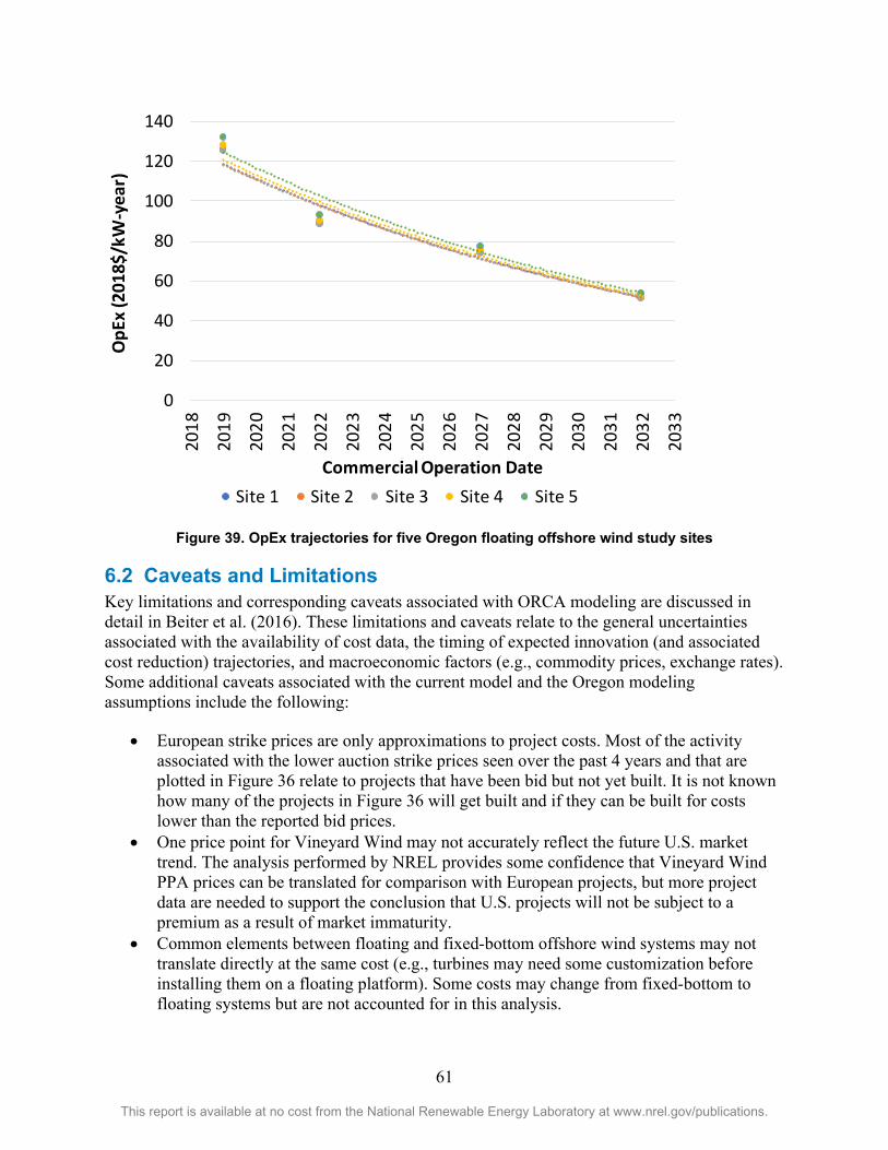
61
This report is available at no cost from the National Renewable Energy Laboratory at www.nrel.gov/publications.
Figure 39. OpEx trajectories for five Oregon floating offshore wind study sites
6.2 Caveats and Limitations Key limitations and corresponding caveats associated with ORCA modeling are discussed in detail in Beiter et al. (2016). These limitations and caveats relate to the general uncertainties associated with the availability of cost data, the timing of expected innovation (and associated cost reduction) trajectories, and macroeconomic factors (e.g., commodity prices, exchange rates). Some additional caveats associated with the current model and the Oregon modeling assumptions include the following:
• European strike prices are only approximations to project costs. Most of the activity associated with the lower auction strike prices seen over the past 4 years and that are plotted in Figure 36 relate to projects that have been bid but not yet built. It is not known how many of the projects in Figure 36 will get built and if they can be built for costs lower than the reported bid prices.
• One price point for Vineyard Wind may not accurately reflect the future U.S. market trend. The analysis performed by NREL provides some confidence that Vineyard Wind PPA prices can be translated for comparison with European projects, but more project data are needed to support the conclusion that U.S. projects will not be subject to a premium as a result of market immaturity.
• Common elements between floating and fixed-bottom offshore wind systems may not translate directly at the same cost (e.g., turbines may need some customization before installing them on a floating platform). Some costs may change from fixed-bottom to floating systems but are not accounted for in this analysis.
0
20
40
60
80
100
120
140
2018
2019
2020
2021
2022
2023
2024
2025
2026
2027
2028
2029
2030
2031
2032
2033
OpE
x (2
018$
/kW
-yea
r)
Commercial Operation DateSite 1 Site 2 Site 3 Site 4 Site 5

62
This report is available at no cost from the National Renewable Energy Laboratory at www.nrel.gov/publications.
• Floating cost assumptions do not include an Atlantic-to-Pacific adjustment. The supply chains in the Pacific may have different constraints and advantages, such as better access to Asian markets, that have not been accounted for.
• Floating-specific component costs based on vendor quotes and production cost estimates may not represent actual costs when built. Most floating cost data have higher uncertainty because values are based on production cost estimates rather than realized costs.
• Wind resource estimates from the WIND Toolkit are the best available but have not been validated against observations and have associated uncertainty. Better resource data is needed to verify AEP assumptions.
• Grid connections in Oregon may prove to be difficult when injecting 600 MW of power at a single location. Transmission upgrades may be necessary to deliver the power but may be challenging and costly. Conversely, some grid system costs may potentially be avoided by using offshore wind development to reduce congestion in some locations, but understanding these issues is beyond the scope of this study.
• Turbine growth may be hindered by unforeseen technology issues. For example, 15-MW wind turbines will be technologically challenging, and their development is not a certainty.
• ORCA is undergoing upgrades related to balance of system and O&M, and its characterization of turbine scaling and AEP profiles. All of these model elements require further development.
• Research is needed to further validate key assumptions of this study, particularly to evaluate the degree to which learning and supply chain expertise from the U.S. Atlantic Coast and Asia (and the fixed-bottom industry) can be leveraged for building a robust floating offshore wind supply chain along the Oregon and Pacific Coast. As more data become available about the evolving technology and cost trajectory of the global and U.S. floating wind industry, costs will need to be calibrated.

63
This report is available at no cost from the National Renewable Energy Laboratory at www.nrel.gov/publications.
7. Summary and Conclusions This study focused on assessing the present and future costs of floating offshore wind technology deployment in the state of Oregon at commercial scale. The study was performed by NREL and funded by BOEM. The study builds off a previous report published by NREL and BOEM in December 2016, titled “Potential Offshore Wind Energy Areas in California: An Assessment of Locations, Technology, and Costs” (Musial et al. 2016a), also funded by BOEM, which estimated LCOE for floating offshore wind in California at $100/MWh or less by 2030.
Since 2016, when the California study was conducted, fixed-bottom and floating offshore wind systems have progressed at a rapid rate both technologically and economically. There are several key areas that were not considered in the California report that are now known to be important variables in estimating future costs of floating wind in general, and in Oregon specifically. Some of the major new areas that were considered in the latest version of ORCA include:
• Strike price declines by about 65% for projects being commissioned between 2017 and 2025 in European auctions for offshore wind (Beiter et al. 2017).
• A new U.S. price point for fixed-bottom offshore wind, established through analysis of the Vineyard Wind PPAs (Beiter et al. 2019).
• Lower-than-expected Vineyard Wind PPA prices, which indicate minimal cost penalties because of immature U.S. supply chains (Beiter et al. 2019).
• Finance costs were reassessed and are lower than previously anticipated based on new industry data (Green Giraffe 2016).
• NREL’s cost model, ORCA, was updated to look ahead to 2032 (previously 2027, extrapolating to 2030).
• Turbine power capacity is assumed to reach 15 MW within the modeling time horizon of 2032 (General Electric 2018; Hundleby et al. 2017).
• Turbine costs per kilowatt were adjusted downward and are not expected to increase as turbine sizes grow.
• Optimized floating platform designs promise a lower component cost for platforms, and systemwide benefits to reduce labor at sea and commissioning time (Villaespesa et al. 2015; Melis et al. 2016). Platform scaling also shows favorable cost declines for larger platform sizes.
Five study sites were selected in Oregon that represent typical locations where offshore wind projects could be built and were analyzed to estimate the cost of offshore wind. This site-selection process was conducted to model potential cost. This study is not stakeholder engagement or a marine spatial planning effort to create wind energy areas under BOEM’s leasing process and the hypothetical sites have not been vetted by ocean user communities. Any wind energy planning effort on the OCS would require comprehensive stakeholder engagement and analysis of all relevant data and information for siting.
We analyzed floating offshore wind costs at each of the five study sites using a version of the ORCA model and incorporating updated modeling assumptions for a 600-MW project at commercial scale.
The results of this cost study estimate that LCOE could range from $74 MWh to $53/MWh in Oregon for floating wind technology in 2032. These results are based on assessments for all five

64
This report is available at no cost from the National Renewable Energy Laboratory at www.nrel.gov/publications.
sites using a conceptual NREL-designed 15-MW wind turbine. These costs reflect lower LCOE than the 2016 California study because of new cost and technology data that support lower CapEx and OpEx than was previously modeled.
We compared full-scale 600-MW project costs for a site near Coos Bay, Oregon, to a 24-MW pilot-scale Principle Power, Inc., project proposed in 2014, also off Coos Bay. The pilot-scale project costs were three times higher than the commercial-scale project using the same financing and energy production. This analysis demonstrated the benefits of building projects at commercial scale.
Overall, the prospects for offshore wind in Oregon look promising for large-scale electricity generation. Floating technology is maturing rapidly, and offshore wind can provide a carbon-free alternative electricity source in coastal regions, especially in the southern region where offshore annual average wind speeds are near 10 m/s and among the highest in the United States. However, wind resource assessments are based on single ensemble setups and validations are sparse; therefore, higher-resolution resource data are needed to lower uncertainty for investors, lawmakers, developers, and utilities that are considering offshore wind in Oregon.
There will be significant challenges for offshore wind to overcome in Oregon including optimization of floating technology, coexistence with the fishing industry, mitigating impacts to wildlife and the viewshed, and integrating with the existing land-based grid. However, offshore wind can play a long-term role in helping to meet state and regional electricity-generation goals and could be synergistic in relieving congestion at some grid locations. Future work should focus on assessing these potential impacts to allow for offshore wind development to progress in a manner that is appropriate and fair for all stakeholder communities.

65
This report is available at no cost from the National Renewable Energy Laboratory at www.nrel.gov/publications.
References ABB Energy Velocity Suite. 2019a. “Electric Substations dataset (2019).” Licensed by NREL. Accessed April 2019.
ABB Energy Velocity Suite. 2019b. “Transmission Lines dataset (2019).” Licensed by NREL. Accessed April 2019.
AWS Truepower, LLC. 2010. OpenWind Theoretical Basis and Validation. http://www.awsopenwind.org/downloads/documentation/OpenWindTheoryAndValidation.pdf
AWS Truepower. 2012. “Wind Resource Maps and Data: Methods and Validation.” https://www.awstruepower.com/products/maps-and-resource-data. Accessed July 2016. AWS Truepower. 2014. AWS Truepower Loss and Uncertainty Methods. Memorandum. June 5, 2014. https://www.awstruepower.com/assets/AWS-Truepower-Loss-and-Uncertainty-Memorandum-5-Jun-2014.pdf.
Bak, C., Zahle, F., Bitsche, R., Kim, T., Yde, A., Henriksen, L. C., Natarajan, A. 2013. The DTU 10 MW Reference Wind Turbine. Danish Technical University. http://orbit.dtu.dk/files/55645274/The_DTU_10MW_Reference_Turbine_Christian_Bak.pdf.
Banister, Kevin. 2017. WindFloat Pacific Project, Final Scientific and Technical Report. United States. doi:10.2172/1339449. https://www.osti.gov/servlets/purl/1339449.
Beiter, P., W. Musial, A. Smith, L. Kilcher, R. Damiani, M. Maness, S. Sirnivas, T. Stehly, V. Gevorgian, M. Mooney, Scott G. 2016. A Spatial-Economic Cost Reduction Pathway Analysis for U.S. Offshore Wind Energy Development from 2015–2030 (Technical Report). Golden, CO: National Renewable Energy Laboratory. NREL/TP-6A20-66579. https://www.nrel.gov/docs/fy16osti/66579.pdf.
Beiter, Philipp, Walter Musial, Levi Kilcher, Michael Maness, and Aaron Smith. 2017. An Assessment of the Economic Potential of Offshore Wind in the United States from 2015 to 2030. Golden, CO: National Renewable Energy Laboratory. NREL/TP-6A20-67675. https://www.nrel.gov/docs/fy17osti/67675.pdf.
Beiter, Philipp, Walter Musial, and Eric Lantz. 2019. The Vineyard Wind Power Purchase Agreement: Insights for Estimating Costs of U.S. Offshore Wind Projects (Technical Report). Golden, CO: National Renewable Energy Laboratory. NREL/TP-5000-72981. https://www.nrel.gov/docs/fy19osti/72981.pdf.
Black & Veatch. 2010. “Technology Characterization for Renewable Energy Electricity Futures Study: GIS Database of Offshore Wind Resource Competing Uses and Environmentally Sensitive Areas.” Overland Park, KS: Black & Veatch (unpublished).
Bonneville Power Administration (BPA). 2019. BPA Website https://www.bpa.gov/Pages/home.aspx.

66
This report is available at no cost from the National Renewable Energy Laboratory at www.nrel.gov/publications.
Bureau of Ocean Energy Management (BOEM). 2018. “Renewable Energy Path Forward on the Atlantic.” Request for Information, Aug 2018. https://www.boem.gov/Renewable-Energy-Path-Forward. BOEM. 2019a. “California Activities.” Accessed April 2019. https://www.boem.gov/California/.
BOEM. 2019b. “Hawaii Activities.” Accessed April 2019. https://www.boem.gov/Hawaii/. Bureau of Ocean Energy Management and National Oceanic and Atmospheric Administration. 2013. “Vessel Traffic Data.” www.marinecadastre.gov.
Chee, Foo Yun. 2018. “Goldman Sachs, Prysmian, others lose challenge against EU cartel fine.” Reuters. Accessed July 2, 2019. https://www.reuters.com/article/us-eu-cartel-court/goldman-sachs-prysmian-others-lose-challenge-against-eu-cartel-fine-idUSKBN1K21DY.
Davis, C. 2015. “Without Oregon utilities nod, Coos Bay WindFloat dead in the water.” The World. https://theworldlink.com/news/local/without-oregon-utilities-nod-coos-bay-windfloat-dead-in-the/article_095e12ca-6d7e-53e0-a313-05181d324cf3.html.
Deepwater Wind. 2015. “Block Island Wind Farm Now Fully Financed.” Accessed July 2019. http://dwwind.com/press/block-island-wind-farm-now-fully-financed.
Draxl, Caroline, Andy Clifton, Bri-Mathias Hodge, James McCaa. 2015. “The Wind Integration National Dataset (WIND) Toolkit.” Applied Energy. 151(1):355-366. ISSN 0306-2619. http://dx.doi.org/10.1016/j.apenergy.2015.03.121.
Efstathiou, Jim. 2018. “First Big U.S. Offshore Wind Farm Offers $1.4 Billion to Customers.” Bloomberg New Energy Finance, August 1, 2018. https://www.bloomberg.com/news/articles/2018-08-01/first-big-u-s-offshore-wind-offers-1-4-billion-to-customers.
General Electric. 2018. “Haliade-X Offshore Wind Turbine Platform.” Accessed December 31, 2018. https://www.ge.com/renewableenergy/wind-energy/turbines/haliade-x-offshore-turbine.

67
This report is available at no cost from the National Renewable Energy Laboratory at www.nrel.gov/publications.
Gilman, P., B. Maurer, L. Feinberg, A. Duerr, L. Peterson, W. Musial, P. Beiter, J. Golladay, J. Stromberg, I. Johnson, D. Boren, A. Moore. 2016. National Offshore Wind Strategy: Facilitating the Development of the Offshore Wind Industry in the United States. U.S. Department of Energy and Bureau of Ocean Energy Management. http://energy.gov/sites/prod/files/2016/09/f33/National-Offshore-Wind-Strategy-report-09082016.pdf.
Green Giraffe. 2016. “Offshore wind finance –2016 update.” Presented at Energy Talk, December 8, 2016, London, England. Accessed March 2018. https://green-giraffe.eu/sites/green-giraffe.eu/files/161206_energytalk_v5_-_sent_orga.pdf.
Guillet, Jerome. 2018. “Who will fund U.S. Offshore Wind - and on what terms?” Presented at the Offshore Wind Implementation Summit, September 7, 2018, Teaneck, New Jersey. https://green-giraffe.eu/presentations/who-will-fund-us-offshore-wind-%E2%80%93-and-what-terms.
Hundleby, Giles, Kate Freeman, Andy Logan, and Ciaran Frost. 2017. “Floating Offshore: 55 Technology Innovations That Will Have Greater Impact on Reducing the Cost of Electricity from European Floating Offshore Wind Farms.” KiC InnoEnergy and BVG Associates. http://www.innoenergy.com/new-floating-offshore-wind-report-55-technology-innovations-that-will-impact-the-lcoe-in-floating-offshore-wind-farms/.
Maness M., B. Maples, and A. Smith, A. 2017. NREL Offshore Balance-of-System Model (Technical Report). Golden, CO: National Renewable Energy Laboratory.NREL/TP-6A20-66874.https://www.nrel.gov/docs/fy17osti/66874.pdf.
Melis, C., C. Bauduin, A. Wattez, A. Newport, Y. Poirette, T. Perdrizet, T., et al. 2016. “Adapting tension leg technology to provide an economical solution for floating wind power.” In: Offshore Technology Conference. OTC-27153-MS; 2016.
MHI Vestas. 2018. “Vineyard Wind Selects MHI Vestas as Preferred Supplier for First Large-scale Offshore Wind Project in the United States.” November 27, 2018. http://www.mhivestasoffshore.com/vineyard-wind-selects-mhi-vestas-as-preferred-supplier.
MHI Vestas. 2019 “MHI Vestas To Supply Five V164-9.5 MW Turbines for Kincardine Floating Offshore Wind Park in Scotland.” http://www.mhivestasoffshore.com/mhi-vestas-to-supply-five-v164-9-5-mw-turbines-for-kincardine-floating-offshore-wind-park-in-scotland.
Musial, W. and B. Ram. 2010. Large-Scale Offshore Wind Power in the United States: Assessment of Opportunities and Barriers (Technical Report). Golden, CO: National Renewable Energy Laboratory. NREL/TP-500-40745. http://www.nrel.gov/docs/fy10osti/40745.pdf.

68
This report is available at no cost from the National Renewable Energy Laboratory at www.nrel.gov/publications.
Musial, Walt, Philipp Beiter, Suzanne Tegen, and Aaron Smith. 2016a. Potential Offshore Wind Energy Areas in California: An Assessment of Locations, Technology, and Costs (Technical Report). Golden, CO: National Renewable Energy Laboratory. NREL/TP-5000-67414. https://www.boem.gov/2016-074/.
Musial, W., D. Heimiller, P. Beiter, G. Scott, and C. Draxl. 2016b. 2016 Offshore Wind Energy Resource Assessment for the United States (Technical Report). Golden, CO: National Renewable Energy Laboratory. NREL/TP-5000-66599. http://www.nrel.gov/docs/fy16osti/66599.pdf.
Musial, W, P. Beiter, P. Spitsen, J. Nunemaker, V. Gevorgian. 2019. 2018 Offshore Wind Technologies Market Report. U.S. Department of Energy, Washington, D.C. https://www.energy.gov/eere/wind/2018-wind-market-reports#offshore. National Geospatial Intelligence Agency. Undated. “World Port Index (2017).” Dataset. https://msi.nga.mil/NGAPortal/MSI.portal?_nfpb=true&_pageLabel=msi_portal_page_62&pubCode=0015. Accessed March 2017.
National Oceanic and Atmospheric Administration (NOAA). 2018. “State Waters and Federal Waters Boundary dataset.” Produced by the NOAA Office of Coast Survey, NOAA Office of Coastal Management, BOEM Mapping and Boundaries Branch, and Department of the Interior Minerals Management Service. Distributed at http://www.nauticalcharts.noaa.gov/csdl/mbound.html. Accessed April 2019.
NOAA National Marine Fisheries Service. 2019a. “West Coast Bottom Trawl Fishing Intensity (2006-2010).https://coast.noaa.gov/digitalcoast/data. Accessed April 2019. NOAA National Marine Fisheries Service. 2019b. “West Coast Mid-Water Trawl Fishing Intensity (2006-2010).” https://coast.noaa.gov/digitalcoast/data. Accessed April 2019.
NOAA Marine Protected Areas Center. 2019. “Marine Protected Areas.” https://marineprotectedareas.noaa.gov/dataanalysis/mpainventory/mpaviewer/.
NOAA Fisheries. 2019. “Leatherback Sea Turtle Critical Habitat Map - West Coast.” https://www.fisheries.noaa.gov/resource/map/leatherback-sea-turtle-critical-habitat-map-west-coast.
North American Submarine Cable Association. 2019. “Submarine Cables dataset (2015).” Distributed by the NOAA Office for Coastal Management. https://marinecadastre.gov/data. Accessed April 2019.
Oregon Department of Energy 2019. “Electricity Mix in Oregon.” https://www.oregon.gov/energy/energy-oregon/Pages/Electricity-Mix-in-Oregon.aspx. Accessed June 4, 2019.
PBS Learning Media. 2019. “Population Map of Oregon.” https://rmpbs.pbslearningmedia.org/resource/great-states-oregon-1.3/activity.

69
This report is available at no cost from the National Renewable Energy Laboratory at www.nrel.gov/publications.
Porter, A., and Phillips, S. 2016. “Determining the Infrastructure Needs to Support Offshore Floating Wind and Marine Hydrokinetic Facilities on the Pacific West Coast and Hawaii.” U.S. Department of the Interior, Bureau of Ocean Energy Management, Pacific OCS Region, Camarillo, CA. OCS Study BOEM 2016-011. 238 pp. https://www.boem.gov/BOEM-2016-011/.
Roberts, D. 2019. “Oregon is poised to set a cap on greenhouse gas emissions. That’s a huge deal.” Vox. June 5, 2019. https://www.vox.com/energy-and-environment/2019/6/5/18650155/climate-change-oregon-carbon-cap-trade-california. Siemens Gamesa. 2019. “Siemens Gamesa launches 10 MW offshore wind turbine; annual energy production (AEP) increase of 30% vs. predecessor.” https://www.siemensgamesa.com/en-int/newsroom/2019/01/new-siemens-gamesa-10-mw-offshore-wind-turbine-sg-10-0-193-dd.
State of Oregon. 2019. “State of Oregon Geographic Location Description: Analysis of Reasonably Foreseeable Effects of Federal Actions Related to Marine Renewable Energy Projects on Resources and Uses Occurring within the Federal Waters of the Oregon Ocean Stewardship Area.” Oregon Department of Land Conservation and Development, Coastal Management Program. https://www.oregon.gov/lcd/OCMP/Documents/OCMP_MarineRenewable_GLD_final.pdf.
Sullivan, Robert G., Leslie B. Kirchler, Jackson Cothren, and Snow L. Winters. 2012. “Offshore Wind Turbine Visibility and Visual Impact Threshold Distances.” .Argonne National Laboratory. http://blmwyomingvisual.anl.gov/docs/EnvPractice_Offshore%20Wind%20Turbine%20Visibility%20and%20Visual%20Impact%20Threshold%20Distances.pdf.
U.S. Department of Energy. 2015. Wind Vision: A New Era for Wind Power in the United States. U.S. Department of Energy Office of Energy Efficiency and Renewable Energy. DOE/GO-102015-4557. Washington, D.C. http://www.energy.gov/sites/prod/files/WindVision_Report_final.pdf. Accessed May 2019.
U.S. Department of Energy. 2019. “DOE Advanced Technology Demonstration Projects.” https://www.energy.gov/eere/wind/offshore-wind-advanced-technology-demonstration-projects.
Valpy, B., P. English, Philip, A. Martínez, E. Simonot. 2014. Future renewable energy costs: offshore wind. BVG Associates and KIC InnoEnergy. Accessed June 6, 2016. http://www.kic-innoenergy.com/wp-content/uploads/2014/09/KIC_IE_OffshoreWind_anticipated_innovations_impact1.pdf.
Villaespesa, E. B., Gonzalez, C. M., Martin, N. G. K. 2015. Transportation and installation of the Tetraspar floating offshore wind turbine. Tech. Rep.; Aalborg University; Aalborg, Denmark; 2015. https://projekter.aau.dk/projekter/files/281663582/Master_Thesis.pdf.
Westington, M., and Slagel, M. 2019. “U.S. Maritime Zones and the Determination of the National Baseline.” National Ocean Service (NOAA) Office of Coast Survey. http://ushydro.thsoa.org/hy07/11_01.pdf.

70
This report is available at no cost from the National Renewable Energy Laboratory at www.nrel.gov/publications.
Weston, D. 2019. “Stiesdal’s TetraSpar demo gets go-ahead.” WindPower Offshore. February 13, 2019. https://www.windpoweroffshore.com/article/1525677/stiesdals-tetraspar-demo-gets-go-ahead.
Wind Europe. 2018. “Floating Offshore Wind Energy: A Policy Blueprint for Europe.”https://windeurope.org/wp-content/uploads/files/policy/position-papers/Floating-offshore-wind-energy-a-policy-blueprint-for-Europe.pdf.
Wiser, R., K. Jenni, J. Seel, E. Baker, M. Hand, E. Lantz, A. Smith. 2016. Forecasting Wind Energy Costs & Cost Drivers. The Views of the World’s Leading Experts. LBNL-1005717. Lawrence Berkeley National Laboratory. http://eta-publications.lbl.gov/sites/default/files/lbnl-1005717.pdf.

71
This report is available at no cost from the National Renewable Energy Laboratory at www.nrel.gov/publications.
Appendix A. Principle Power Project Scaling Study The cost of offshore wind is sensitive to technological and spatial variables, including average wind speed, turbine size, water depth, and project scale, to name a few. Project scale is difficult to demonstrate as a cost driver because the large financial investments (greater than $1 billion) needed to build an economical commercial-scale project is often prohibitive, especially for new technology. However, smaller investments at a pilot scale most often come at a higher cost per unit of energy. Nevertheless, with the nascent state of floating wind technology, it is prudent to demonstrate this new technology initially at a pilot scale.34 However, investors will not be satisfied unless they are convinced that a lower unit cost can be achieved at commercial scale. This section examines a case study relevant to the state of Oregon for offshore wind. Principle Power, Inc., a leading offshore wind floating platform technology developer, provided detailed costs for a pilot project to the Oregon Public Utility Commission in 2014 off the coast of Coos Bay, Oregon, which were rejected because the project was deemed too expensive. Here, we compare that pilot-scale project to the cost of a commercial-scale project (e.g., 600 megawatts [MW]) in the same location using current technology (Banister 2017).
Background and Coos Bay Project Description The National Renewable Energy Laboratory (NREL) obtained cost information from Principle Power, Inc. on their proposed 24-MW Advanced Technology Demonstration pilot project off Coos Bay, Oregon, to allow for comparison with the commercial projects analyzed in this report. Figure A-1 shows the first Principle Power, Inc. prototype being towed to its station off Portugal in 2011.
Figure A-1. Principle Power, Inc. semisubmersible with mounted turbine. Photo courtesy of Principle
Power, Inc.
34 A pilot scale is subjectively defined. In this report, pilot scale means the project is using state-of-the-art turbine technology but in smaller numbers, usually less than 50 MW total capacity. Pilot-scale projects are privately financed but are not economically viable without some public or private subsidies.

72
This report is available at no cost from the National Renewable Energy Laboratory at www.nrel.gov/publications.
Offshore wind pilot-scale projects are pursued by technology developers to demonstrate the technical and economic viability of a concept design, improve engineering and related support activities, address nontechnical barriers (e.g., environmental or socio-economic issues), and collect performance, monitoring, and cost data (Banister 2017). According to Banister (2017), the WindFloat Pacific project from Principle Power was “the first floating project offshore wind array proposed in the United States and the first offshore wind project of any kind proposed off the West Coast.”
The cost structure according to Banister (2017) for the WindFloat Pacific project is shown in Table A-1, converted to $2018. The 24-MW project was proposed to be sited at a water depth of 435 meters and a 30-kilometer distance from export cable landfall. This reported capital expenditure (CapEx) estimate from the WindFloat Pacific project compares to an estimated CapEx of $9,700/kilowatts (kW) for the 30-MW Block Island Wind Farm project (Deepwater Wind 2015).35
Table A-1. Cost Breakdown for the 24-MW Principle Power Pacific WindFloat Project
Category Unit Cost Source CapEx $/kW 10,153
Banister (2017) OpEx36 $/kW/year 243 Net Capacity Factor % 43%
Because of the project’s smaller capacity, the costs were higher per-unit CapEx ($/kW) and operation and maintenance ($/kW/year) than a full-scale commercial project. Commercial-scale projects leverage economies of scale by spreading fixed-cost capital and OpEx over a higher number of turbines and total installed capacity. For instance, by spreading the cost of an export system cable infrastructure over many turbines instead of just a few turbines (WindFloat Pacific used three turbines), the per-unit cost ($/kW) is much smaller. For some cost elements, these scaling effects can have several orders of magnitude difference between the pilot-scale and the commercial-scale project, especially for offshore wind projects, because they have higher upfront CapEx.
Project-Scale Cost Comparisons Table A-2 shows the comparison between the 24-MW WindFloat Pacific project and the 600-MW project (Section 6), with a 2032 commercial operation date (COD) for the Coos Bay location (south-central; Site 4). These calculations were informed by cost information obtained from Principle Power, but the component cost data are provided by NREL and are representative of industry costs. NREL cost data from multiple sources are aggregated and presented here to allow the results to be published without revealing proprietary data. The same annual energy production and financing conditions were assumed for this comparison to focus on the scaling effects resulting from differences in plant size. Note that this comparison is made in 2032
35This estimate was derived by dividing the reported project financing of $290 million by the project capacity of 30 MW. 36Operational expenditures

73
This report is available at no cost from the National Renewable Energy Laboratory at www.nrel.gov/publications.
(COD); therefore, these results represent the combined impact from projected cost reductions (by 2032)37 and from economies of scale (24-MW vs. 600-MW project size).
Table A-2. CapEx Estimates for 24-MW and 600-MW Project Scale in 2032 (COD)
The input data show that estimated CapEx ($/kW) is 67% lower for the 600-MW project size relative to the 24-MW project. A similar magnitude of difference (-70%) was estimated for
37 The same cost reductions were applied to the 24-MW and 600-MW projects to estimate costs in 2032 (COD).
Project size Unit
600 MW Project Size 24 MW Project Size $/kW $/kW % Difference
1 Tower 182 250 -27% 2 RNA 839 1,536 -45% TURBINE SUPPLY 1,021 1,786 -43% 3 Substructure 577 1,265 -54% 4 Foundation1 - - 0% SUPPORT STRUCTURE 577 1,265 -54% 5 Port, Staging, Logistics and Transport 44 868 -95% 6 Turbine Install - - 0% 7 Substructure Install2 164 300 -45% TOTAL INSTALLATION 208 1,169 -82% 8 Array Cabling 181 181 0% 9 Export Cable 253 1,574 -84% 10 Grid Connection 7 7 0% TOTAL ELECTRIC SYSTEM 441 1,762 -75% 11 Development 79 974 -92% 12 Lease Price 88 88 0% 13 Project Management 45 168 -73% BALANCE OF SYSTEM 1,438 5,426 -73% 14 Insurance During Construction 28 72 -61% 15 Project Completion 28 72 -61% 16 Decommissioning 28 175 -84% 17 Procurement Contingency 132 302 -56% 18 Install Contingency 57 351 -84% 19 Construction Financing 118 686 -83% TOTAL SOFT CAPEX 391 1,658 -76% TOTAL CAPEX 2,924 8,870 -67% $/kW-year $/kW-year % Difference 1 Operations 19 64 -70% 2 Maintenance 33 109 -70% TOTAL OPEX 52 172 -70% % % % Difference 1 Net Capacity Factor 47% 47% 0%
NET CAPACITY FACTOR 47% 47% 0% % % % Difference 1 WACC (nominal) 5.4% 5.4% 0%
FIXED CHARGE RATE (nominal) 7.11% 7.11% 0% $/MWh $/MWh % Difference LCOE 63 183 -68%
1 Expenditures for substructure and foundation are combined under the “substructure” line item because of the proprietary nature of the underlying data. 2 Expenditures for turbine and substructure installation are combined under the “substructure installation” line item because of the proprietary nature of the underlying data.

74
This report is available at no cost from the National Renewable Energy Laboratory at www.nrel.gov/publications.
OpEx. In other words, the pilot-scale project CapEx was about three times higher than the commercial-scale project. The levelized cost of energy (LCOE) was modeled to be about three times lower for the 600-MW commercial power plant size compared to the 24-MW pilot project. Quantitatively, economies of scale from plant sizing has the largest effect on installation (-82%) and electric system (-75%) line items, as well as project development and management (-92% and -73%, respectively).
Both the pilot-scale and commercial-scale project were assumed to have the same favorable financing rates and generated power with the same net capacity factor of 44%.
Project Scaling Conclusions In this study, we estimated the cost-scaling relationship between the 24-MW WindFloat Pacific project proposed by Principle Power in 2014 and a 600-MW project located at the same site (Site 4 off Coos Bay, Oregon). The LCOE was approximately three times higher for the 24-MW pilot-scale project. This cost difference mostly reflects the capital and operation cost economies of scale that allow fixed cost items to be spread over the entire project cost. As the comparison is made in model year 2032, the estimated costs shown in Table A-2 also represent technology improvements assumed to be realized since the WindFloat Pacific was originally proposed, such as larger turbines that are assumed to be available in a decade. The LCOE for the pilot-scale project was calculated to be $183/megawatt-hour, whereas the commercial-scale project LCOE was found to be $63/megawatt-hour.

75
This report is available at no cost from the National Renewable Energy Laboratory at www.nrel.gov/publications.
Appendix B. Monthly Wind Resource Site Characteristics The data in Figures B-1 through B-5 show the results of the Windographer analysis of the diurnal wind various for each month at all five study sites.
Figure B-1. Mean diurnal profiles for Site 1

76
This report is available at no cost from the National Renewable Energy Laboratory at www.nrel.gov/publications.
Figure B-2. Mean diurnal profiles for Site 2

77
This report is available at no cost from the National Renewable Energy Laboratory at www.nrel.gov/publications.
Figure B-3. Mean diurnal profiles for Site 3

78
This report is available at no cost from the National Renewable Energy Laboratory at www.nrel.gov/publications.
Figure B-4. Mean diurnal profiles for Site 4

79
This report is available at no cost from the National Renewable Energy Laboratory at www.nrel.gov/publications.
Figure B-5. Mean diurnal profiles for Site 5

80
This report is available at no cost from the National Renewable Energy Laboratory at www.nrel.gov/publications.
Appendix C. Baseline Cost Results A baseline cost analysis was performed for three modeled years, representing commercial operation dates (COD) of 2015, 2022, and 2027. In addition, the resultant baseline levelized cost of energy (LCOE) values for these years were extrapolated (using an exponential curve fit) to 2030 to provide a cost estimate that can be compared to the California cost study. Using the technology assumptions in Table C-1, we modeled a 6-megawatt (MW) turbine for 2015, increasing to 8 MW in 2022, and 10 MW in 2027. Plant size was held constant at 600 MW for all model runs. A fixed charge rate (FCR) of 10.51% was used to represent 2016 financing parameters.
Table C-1. Baseline Turbine Technology Assumptions from Musial et al. (2016a)
Commercial Operations Date 2015 2022 2027 Turbine Rated Power (MW) 6 8 10 Turbine Rotor Diameter (m) 155 180 205 Turbine Hub Height (m) 100 112 136 Turbine Specific Power (W/m2) 318 314 303 Substructure Technology Semisubmersible Semisubmersible Semisubmersible
Figure C-1 shows the power curves for the baseline turbines in the Oregon cost study, which are the same as the ones used in the 2016 California study. It is important to note that the Danish Technical University turbine used to represent the 2022 technology in the primary Oregon analysis is different from the 10-MW National Renewable Energy Laboratory (NREL) reference turbine used for the 2016 California study to represent 2027 technology and the baseline analysis for this report. The NREL 10-MW turbine uses a rotor diameter of 205 m, which reflects a lower specific power of 303 W/m2 than offshore wind rotors of today. This estimation of declining specific power is reasonable given that many land-based turbines already exist with specific power well below 300 W/m2. However, with ultra-large offshore machines, increasing rotor diameter is one of the biggest challenges of upscaling, which makes lower specific power turbines more difficult.

81
This report is available at no cost from the National Renewable Energy Laboratory at www.nrel.gov/publications.
Figure C-1. Power curves for the baseline Oregon floating offshore wind study using California
study assumptions for COD years 2015, 2022, and 2027. Source: Musial et al. 2016a

82
This report is available at no cost from the National Renewable Energy Laboratory at www.nrel.gov/publications.
Table C-2. Baseline Gross Capacity Factors, Losses, Net Capacity Factors, and Net Annual Energy Production (AEPnet) for Oregon Sites
The baseline cost results are plotted in Figure C-2 and shown in Table C-3.
Table C-3. Baseline Cost Results
100-m Hub Height Site 1 Site 2 Site 3 Site 4 Site 5Gross Capacity Factor 43.48% 46.26% 47.20% 50.68% 59.74%
Total Losses 22.84% 24.05% 22.02% 21.86% 20.91%Net Capacity Factor 33.55% 35.13% 36.81% 39.60% 47.25%
AEPnet (GWh) 1,763 1,847 1,934 2,081 2,483
112-m Hub Height Site 1 Site 2 Site 3 Site 4 Site 5Gross Capacity Factor 46.35% 49.28% 50.35% 54.09% 63.01%
Total Losses 21.24% 22.37% 20.48% 20.33% 19.45%Net Capacity Factor 36.51% 38.26% 40.04% 43.09% 50.76%
AEPnet (GWh) 1,919 2,011 2,104 2,265 2,668
125-m Hub Height Site 1 Site 2 Site 3 Site 4 Site 5Gross Capacity Factor 50.67% 53.83% 55.10% 58.99% 68.20%
Total Losses 19.83% 20.88% 19.12% 18.98% 18.16%Net Capacity Factor 40.63% 42.59% 44.57% 47.79% 55.82%
AEPnet (GWh) 2,135 2,238 2,342 2,512 2,934
6 MW 2017
8 MW 2022
10 MW 2027
LCOE ($/MWh) Site 1 Site 2 Site 3 Site 4 Site 5 North North Central Central South Central South
2015 $ 242.46 $ 233.26 $ 220.81 $ 217.53 $ 181.56 2022 $ 179.35 $ 172.36 $ 163.63 $ 160.65 $ 135.61 2027 $ 136.03 $ 130.48 $ 124.26 $ 121.28 $ 103.33 2030 $ 119.54 $ 114.48 $ 109.18 $ 106.06 $ 90.53

83
This report is available at no cost from the National Renewable Energy Laboratory at www.nrel.gov/publications.
Figure C-2. Baseline cost trajectories for five Oregon floating offshore wind study sites
For the five sites in this analysis, the largest driver of LCOE is the wind speed gradient from north to south. At a 114-m hub height, based on data obtained from NREL’s Wind Integration National Dataset Toolkit (Draxl 2015), the mean wind speed increases from 7.84 meters per second to 9.91 meters per second from the north to the south site.
For the 6-MW turbine (2017), LCOE varies from 242 $/megawatt-hour (MWh) at the north site and 182 $/MWh at the south site. In 2030, the extrapolated values show baseline costs that vary between $119/MWh in the north to about $90/MWh in the south. These compare to the California study, which show the Humboldt and Channel Island site costs in 2030 to be $100/MWh and $97/MWh, respectively.

84
This report is available at no cost from the National Renewable Energy Laboratory at www.nrel.gov/publications.
Appendix D. Power Curve Data The data in Table D-1 are plotted for the power curves used in this report.
Table D-1. Data Used To Plot Power Curves in Figure 27 and Figure C-1
Wind Speed (m/s)
NREL Reference 6
MW
NREL Reference 8
MW
NREL Reference 10
MW
DTU Reference 10
MW
NREL Reference
12MW
NREL Reference
15MW 0 0 0 0 0 0 0 1 0 0 0 0 0 0 2 0 0 0 0 0 0 3 0 0 0 0 0 0 4 246 359 471 280 400 499 5 562 812 1059 799 1141 1424 6 1033 1483 1928 1533 2189 2732 7 1691 2407 3125 2506 3581 4469 8 2567 3616 4691 3731 5323 6643 9 3691 5135 6655 5312 7579 9459
10 5092 6976 8858 7287 10397 12975 11 5860 7813 9767 9698 12000 15000 12 6000 8000 10000 10639 12000 15000 13 6000 8000 10000 10649 12000 15000 14 6000 8000 10000 10639 12000 15000 15 6000 8000 10000 10684 12000 15000 16 6000 8000 10000 10642 12000 15000 17 6000 8000 10000 10640 12000 15000 18 6000 8000 10000 10640 12000 15000 19 6000 8000 10000 10653 12000 15000 20 6000 8000 10000 10646 12000 15000 21 6000 8000 10000 10644 12000 15000 22 6000 8000 10000 10641 12000 15000 23 6000 8000 10000 10640 12000 15000 24 6000 8000 10000 10644 12000 15000 25 6000 8000 10000 10636 12000 15000