Ordinary Differential Equations - WordPress.com€¦ · Web viewis called ordinary differential equation. If partial derivatives occur, ... are all first order differential equations

Unit I Ordinary Differential Equations

Ordinary Differential Equations 1.1 Definition and Examples of Differential Equations

Definition 1.1 An ordinary differential equation is an equation that contains one

or several derivatives of an unknown function (of single variable) y(x)

that may contain the function itself and given functions of x.

Example 1 a) = cos x b) x 2 + x + (x 2 4) y = 0

c) d) = 2x y.

If the derivatives that appear in the differential equation are not partial derivatives, then the equation

is called ordinary differential equation. If partial derivatives occur, then the equation is called partial

differential equation.

Thus (a) and (b) are ordinary differential equations while (c) and (d) are partial differential

equations.

Definition 1.2 Order of a D.E.

The order of a differential equation is the order of the highest

derivative which appears in the equation.

Example 2 a) + 4y = is of order 2.

b) x 2 + 2 = (x 2 + 2) y 2 is of order 3.

c) + + = 0 is of order 4.

1.1.1 First Order Differential Equations

First order differential equation contains only and may contain y and given functions of x, hence can

be written as:

F(x, y, ) = 0 (1)

Or = f(x, y)

Example 3 a) cos x = 0 b) x 2y = 0 c) y 2x = 0

are all first order differential equations.

Prepared by Tekleyohannes Negussie 68


Solution of a Differential Equation

A solution of a given first order differential equation (1) on some open interval a < x < b is a function

y = h(x) that has a derivative = h (x) and satisfies (1) for a < x < b.

Example 4 Show that y = x 2 is a solution of x 2y = 0.

Solution = 2x . Hence x = 2 x 2 = 2 y.

Thus y = x 2 is a solution of x 2y = 0.

Example 5 Show that y = is a solution of y + = 0.

Solution = . Hence y + = = 0.

Thus y = is a solution of y + = 0.

Remark: The solution of a differential equation may appear as an implicit function in the

Form:

H(x, y) = 0

Example 6 is an implicit solution of the differential equation y + x = 0.

Since

Hence H(x, y) = .

Note that: The graph of any solution of a d. e. is called an integral curve.

Example 7 y = sin x + c is a solution of = cos x. For different c we get the following curves.

Prepared by Tekleyohannes Negussie

x

y

for c = 0

69


General and Particular Solutions

Solutions of d. e. that involves an arbitrary constant c are called general solutions and if we choose

specific constant c*, we obtain what is called a particular solution of the d. e.

Example 8 = cos x.

y (x) = sin x + c is a general solution while y (x) = sin x + is a particular solution.

1.1.2 Initial Value Problems

Given the first order differential equation

= f (x, y) with additional condition y ( ) = .

The additional condition y ( ) = is called an initial condition.

A differential equation together with an initial condition is called an initial value problem. The initial

condition is used to determine the value of the arbitrary constant c.

Example 9 = 2x, y (2) = 1.

The general solution is y = + c and from the initial condition y (2) = 4 + c = 1 c = 3.

Therefore, the solution of the initial value problem is y = x 2 3.

Example 10 = 2xy, y (1) = e.The general solution is y = c and from the initial condition y (1) = e c e = e c = 1.

Therefore, the solution of the initial value problem is y = .

Example 11 = y, y (0) = 2.The general solution is y = c and from the initial condition y (0) = 2 c = 2.Therefore, y = 2 is the solution of the given initial value problem. Example 12 = x, y (0) = 3.

The general solution is y = x 2 + c and from the initial condition y (0) = 3 c = 3.

Therefore, y = x 2 + 3 is the solution of the given initial value problem.

1.2 Finding Solutions of Differential Equations

1.2.1 Separable Differential Equations

Many first order differential equations can be reduced to the form:

g(y) = f(x) (1)

This can also be written as:

g(y) dy = f(x) dx. (2)



Since the variables x and y in the above equations are separated, we call such equations separable

differential equations.

An equation of the form (1) can be solved by integration.

(3)

(3) is the general solution of (1).

Example 13 Solve the d. e.

a) 9y + 4x = 0 b) (1 y 2) dx = y (1 x) dy

Solutions a) 9y + 4x = 0 9y dy = 4x dx

y 2 = 2 x 2 + c

+ = c

Thus + = c where c 0, is the general (implicit) solution of the d. e.

b) (1 y 2) dx = y (1 x) dy

=

=

where = 2 c.

= 1 y 2 = (1 x) 2

Now let c0 = .Therefore, (1 x) 2 + y 2 =1 for some c0 , is the general solution of the d. e.

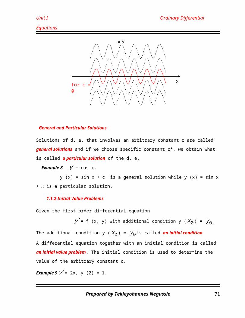
Example 14 Solve the following initial value problems.

a) y = ay; y (0) = 3 and a is a constant.

b) + = 0 and y (0) = 1.

Solutions a) = ay; y (0) = 3.

= ay



y =

y = c , where c =

Now y (0) = 3 c = 3.

Therefore, y = 3 is the solution of the initial value problem.

b) + = 0

+ 5x4y2 = 0 =

y =

Now y (0) = 1 c0 = 1.

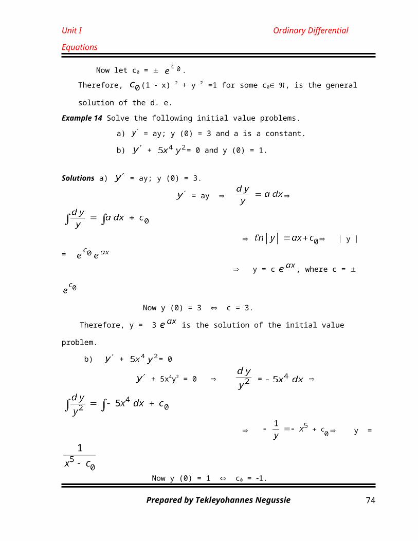
Therefore, y = is the solution of the initial value problem.

Example 15 Find the general solution for the differential equation

= r(y a) (y b) where r, a and b are constants.

Solution = r(y a) (y b)

=

y =

Therefore, y = is the general solution.

Exponential Growth and Exponential Decay

In exponential growth and decay the rate of change of the substance at time t is proportional to the

amount y (t) of the substance present. i.e. is proportional to y.

for some k (1)



The general solution of (1) is of the form y = c e kt.

Exponential growth where k 0 and Exponential decay where k 0

Example 16 Assume that a radioactive substance is under consideration for each time t, let

N (t) denotes the amount of this substance present at time t. N´ (t) is proportional to N (t).

Find the solution to the initial value problem.

N´ (t) = k N (t) and No (t) = No.

Solution The solution is given by

N (t) = c e kt for some k 0.

From No (t) = No we get c = No e k t .

Therefore, the solution of the initial value problem is N (t) = No e (t to) kt.

Example 17 A radioactive substance decomposes at a rate proportional to the amount present.

Starting from a given amount of substance say m grams, at a certain time t = to what can be

said about the amount available at a later time?

Solution N’(t) = k N (t) and (t) = m where k 0.

The general solution is given by N (t) = c e kt.

From (t) = m we get c = m e k to.

Therefore, the solution is N (t) = m e (t to) k.

Example 18 Newton’s Law of Cooling.

A copper ball is heated to a temperature of 100 o c. Then at time t = 0 it is placed in water that is

maintained at a temperature of 30 o c. At the end of 3 min. the temperature of the ball reduced to

70 o c. Find the time at which the temperature of the ball is reduced to 31 o c.

Solution Let T denotes the temperature of the ball at any time t. Then is proportional to

(T ) where is the temperature of the surrounding medium.

Thus = k (T To) ℓn T To = k t + c1 T = To + c e kt.

But at t = 0, T (0) = 100 and = 30. Thus 100 = c + 30 c = 70.

Now let us determine k.

T(t) = 30 + 70 e kt and at t = 3 min. T(3) = 70 and hence 70 = 30 + 70 e 3k.

e 3k = k = ℓn ( ).

Thus, k 0.186538596.

Therefore, T(t) = 70 e 0.186538596 t + 30.



Now T(t) = 31 1 = 70 e 0.186538596 t e 0.186538596 t =

ℓn ( ) = ℓn ( ) ℓn ( ) = ℓn (70)

t 22.775422

Therefore, t 22.78 min.

1.3 Optional Reduction to Separable Form

Certain first order differential equations can be made separable by simple change of variables. This

holds for equation of the form:

= g ( ) where g is any function of .

Set u = . Then y = u x. = u + x u´ where u´ = .

Thus g (u) = x u´ + u

Exercises Solve:

1. 2xy y y2 + x2 = 0. 2. = +

3. (2x 4y + 5) + x + 2y + 3 = 0.

1.4 Exact Differential Equations

In this section we consider differential equation of the form:

M (x, y) + N (x, y) = 0 (1)

which is also written as:

M (x, y) dx + N (x, y) dy = 0 (2)

An equation of the form (1) or (2) is called exact if there is a function U (x, y), with continuous

partial derivatives, such that

= M and = N.

If there exists such a function U (x, y) , then (1) can be written as

dx + dy = 0 (3)

But (3) is called the total differential, du of U (x, y) = c, constant.

i.e. du = dx + dy = 0



The general solution (implicit solution) of the differential equation (1), if it exists, is given by the

form:

U (x, y) = c0

Example 19 Show that every separable differential equation is exact.

Solution A separable differential equation has the form:

g (y) + f (x) = 0 g (y) dy = f (x) dx (4)

Now let U (x, y) = . Then = f (x) and = g (y).

Therefore, (4) is exact.

Theorem 4.1 If M, N and their first partial derivatives are continuous in a

rectangular region in a plane, then equation (1) is exact if and only if

=

If (1) is exact, the function U (x, y) can be found in the following ways.

i) U (x, y) = , where k (y) is a constant of integration.

To determine k (y) we use = + = N (x, y)

where G (x, y) =

ii) U (x, y) = , where l (x) is a constant of integration.

To determine l (x) we use = + = M (x, y)

where F (x, y) =

Example 20 Show that the differential equation is exact and find the

general solution.

Solution M (x, y) = and N (x, y) = .

Both M and N are continuous and have continuous partial derivatives on R.

Hence, by theorem 4.1, the given differential equation is exact if and only if

= .

But = 4x3y = .

Thus the given differential equation is exact.

To find the general solution



U (x, y) = = = + k (y)

and N (x, y) = = +

= 0 k (y) = c1 , constant.

Hence the general solution is given by:

U (x, y) = c0 + c1 = c0 = 2 ( c0 c1) = c

Therefore, the general solution is given by:

= c.

Example 21 Initial Value Problem

Solve the initial value problem

(sin x cosh y) dx (cos x sinh y) dy = 0; y (0) = 0.

Solution M (x, y) = sin x cosh y and N (x, y) = cos x sinh y.

Now = sin x sinh y and = sin x sinh y.

Hence = .

Therefore, the differential equation is exact.

Now U (x, y) = =

= cos x cosh y + l (x).

Since sin x cosh y = = sin x cosh y + l (x), l (x) = 0.

Thus l (x) = c1, constant.

Hence the general solution of the differential equation is:

U (x, y) = c0.

cos x cosh y + c1 = c0. cos x cosh y = c1 c0 = c.

From the initial condition y (0) = 0 we get:

c = 1, since cos 0 = cosh 0 = 1.

Therefore, the solution of the initial value problem is:

cos x cosh y = 1.

Exercises 2 Given U (x, y) = c, find the exact differential equation du = 0.

a) x2 + y2 = U (x, y) b) ℓn (x2y2) = U (x,y)

c) cos ( x2 y2) = U (x, y) d) cosh (x3 y) = U (x, y)



Exercises 3 Solve the following differential equations.

a) b)

c) d) sin y (y x cos y) = 0

e) = 0 f) 4y2 + 8xy = 0: y (3) =

g) ℓn (1 + y2 ) dx +

h) 2 sin y cos y = 0 ; y (0) =

i) 2 xy = x2 + y2; y (1) = 2.

j) (2xy3 ye x ) dx + (3x2y2 + e x 4) dy = 0

Integrating Factor

Given the differential equation

P (x, y) dx + Q (x, y) dy = 0 (1)

that is not exact.

If there is a function F (x, y) such that

F P dx + F Q dy = 0 (2)

is exact, then we call the function F (x, y) an integrating factor of (1).

Example 22 The differential equation y dx x dy = 0 is not exact.

But if we multiply by F (x, y) = , then the differential equation

is exact. (Verify!).

Hence F (x, y) = is an integrating factor.

How to find integrating factors

Integrating factors can be found by:

i) inspection

or ii) using the fact that equation (2) is exact.

Now (2) is exact implies that .

Fy P + F Py = Fx Q + F Qx. (*)



In general (*) would be difficult to solve.

Hence we need to look for an integrating factor depending on one variable. i) If F (x, y) = F (x), then Fx = F and Fy = 0.

Thus (*) becomes F .

. (3)

ii) Similarly if F (x, y) = F (y), then (*) becomes

(4)

Hence we have the following theorems.

Theorem 4.2 (Integrating factor F (x)).

If (1) is such that the right hand side of (3), call it , depends only on x, then

(1) has an integrating factor F = F (x) given by:

F (x) = exp .

Theorem 4.3 (Integrating factor F (y)).

If (1) is such that the right hand side of (3), call it , depends only on y, then

(1) has an integrating factor F = F (y) given by:

F (y) = exp .

Example 23 Find an integrating factor for the differential equation

2 sin y2 dx + xy cos y2 dy = 0 and solve.

Solution Let P = 2 sin y2 and Q = xy cos y2.

Now = 4y cos y2 and = y cos y2 .

i) Integrating factor F = F (x).

Thus we can take F (x) = x3.

Hence 2 sin y2 dx + xy cos y2 dy = 0 2 x3 sin y2 dx + x4y cos y2 dy = 0.



Thus, M = 2 x3 sin y2 and N = x4y cos y2 and = 4 x3 y cos y2 = .

Now U (x, y) = = + k (y).

But N = = = 0 k (y) = .

Thus, the implicit solution for the differential equation is:

U (x, y) = + =

= 2( – ) = c

= c.

ii) Integrating Factor F (y)

Therefore, F (y) = .

Now U (x, y) = =

But N = =

= 0 ℓ(x) = .

Thus, the implicit solution for the differential equation is:

U (x, y) = + =

= ( – ) = = c.

Therefore, = c is the general solution.

Example 24 Solve the initial value problem

, y (1) = 2

Solution Let P = 2 xy and Q = .



Now = 2x and = 6x . Thus, the differential equation is not exact.

Let us find integrating factor F = F (y).

.

Thus, M = and N =

and hence, U (x, y) = =

but N = = = . Thus, = k (y) = + .

The general solution of the differential equation is:

U (x, y) = + + = + = c.

From the initial condition y (1) = 2 we get:

C = 24.

Therefore, + = 24 is the solution of the initial value problem.

Ordinary Linear Differential Equations

Linear Differential Equations

A first order differential equation is said to be linear if it can be written as

(1)Note that: Equation (1) is linear in y and where as P and r can be any functions of x.Examples 25 , and are examples of linear differential equations while and are not linear

differential equations.

In (1) if r (x) 0, i.e. , then it is called a homogeneous differential equation;

otherwise it is said to be non-homogeneous.

Now we need to find a formula for the general solution of (1). To do so we proceed by finding a

formula for the general solution of the associated homogeneous differential equation

This can be done as follows:

.Note that: y (0) 0 is the trivial solution of such differential equations.



Example 26 Solve the following:

a) b) , y (0) = 2.

Solutions a)

.

Therefore, is the general solution of the given differential equation.

b)

.

From the initial condition we get:

C = 2.

Therefore, is the solution of the given initial value problem.

To find the solution of the non-homogeneous differential equation we proceed as follows:

(*)

Now put P = P (x) y – r (x) and Q (x) = 1. Thus, and . Consequently, this

differential equation is not exact.

We need to find an integrating factor.

.

Hence, F (x) = is an integrating factor.

Multiplying both sides of the second equation in (*) we get:

(**)

Now and N = . Hence, = =

.

Thus, (**) is exact.Consequently the general solution of (**) and hence (*) is of the form

U (x, y) = , where

U (x, y) = or U (x, y) =



Thus, U (x, y) =

Now M = = y

y =

= ℓ (x) =

Thus, = = c.Therefore, the general solution of the differential equation is

.Example 27 Solve the following linear differential equations.

a) b) , t 0.Solutions a) .

Now put P (x) = – 1 and r (x) = . Then

and .

Therefore, y (x) = is the general solution.

b) , t 0 .

Now put P (t) = and r (t) = . Then =

and .


Documents

Ordinary Differential Equations - WordPress.com€¦ · Web viewis called ordinary differential equation. If partial derivatives occur, ... are all first order differential equations