Embed Size (px)
Citation preview

O R A C L E ® C R Y S T A L B A L L , F U S I O N E D I T I O N
R E L E A S E 1 1 . 1 . 1 . 3
S T A T I S T I C A L G U I D E

Crystal Ball Statistical Guide, 11.1.1.3
Copyright © 1988, 2009, Oracle and/or its affiliates. All rights reserved.
Authors: EPM Information Development Team
The Programs (which include both the software and documentation) contain proprietary information; they are providedunder a license agreement containing restrictions on use and disclosure and are also protected by copyright, patent, andother intellectual and industrial property laws. Reverse engineering, disassembly, or decompilation of the Programs, exceptto the extent required to obtain interoperability with other independently created software or as specified by law, isprohibited.
The information contained in this document is subject to change without notice. If you find any problems in thedocumentation, please report them to us in writing. This document is not warranted to be error-free. Except as may beexpressly permitted in your license agreement for these Programs, no part of these Programs may be reproduced ortransmitted in any form or by any means, electronic or mechanical, for any purpose.
If the Programs are delivered to the United States Government or anyone licensing or using the Programs on behalf of theUnited States Government, the following notice is applicable:
U.S. GOVERNMENT RIGHTS Programs, software, databases, and related documentation and technical data delivered toU.S. Government customers are "commercial computer software" or "commercial technical data" pursuant to theapplicable Federal Acquisition Regulation and agency-specific supplemental regulations. As such, use, duplication,disclosure, modification, and adaptation of the Programs, including documentation and technical data, shall be subjectto the licensing restrictions set forth in the applicable Oracle license agreement, and, to the extent applicable, the additionalrights set forth in FAR 52.227-19, Commercial Computer Software--Restricted Rights (June 1987). Oracle USA, Inc., 500Oracle Parkway, Redwood City, CA 94065.
The Programs are not intended for use in any nuclear, aviation, mass transit, medical, or other inherently dangerousapplications. It shall be the licensee's responsibility to take all appropriate fail-safe, backup, redundancy and other measuresto ensure the safe use of such applications if the Programs are used for such purposes, and we disclaim liability for anydamages caused by such use of the Programs.
Oracle, JD Edwards, PeopleSoft, and Siebel are registered trademarks of Oracle Corporation and/or its affiliates. Othernames may be trademarks of their respective owners.
The Programs may provide links to Web sites and access to content, products, and services from third parties. Oracle isnot responsible for the availability of, or any content provided on, third-party Web sites. You bear all risks associated withthe use of such content. If you choose to purchase any products or services from a third party, the relationship is directlybetween you and the third party. Oracle is not responsible for: (a) the quality of third-party products or services; or (b)fulfilling any of the terms of the agreement with the third party, including delivery of products or services and warrantyobligations related to purchased products or services. Oracle is not responsible for any loss or damage of any sort that youmay incur from dealing with any third party.

Contents
Chapter 1. Welcome . . . . . . . . . . . . . . . . . . . . . . . . . . . . . . . . . . . . . . . . . . . . . . . . . . . . . . . . . . . . . . . . . 7
Introduction . . . . . . . . . . . . . . . . . . . . . . . . . . . . . . . . . . . . . . . . . . . . . . . . . . . . . . . . . . 7
About This Guide . . . . . . . . . . . . . . . . . . . . . . . . . . . . . . . . . . . . . . . . . . . . . . . . . . . . . . 7
Technical Support and More . . . . . . . . . . . . . . . . . . . . . . . . . . . . . . . . . . . . . . . . . . . . . . 8
Chapter 2. Statistical Definitions . . . . . . . . . . . . . . . . . . . . . . . . . . . . . . . . . . . . . . . . . . . . . . . . . . . . . . . . 9
Introduction . . . . . . . . . . . . . . . . . . . . . . . . . . . . . . . . . . . . . . . . . . . . . . . . . . . . . . . . . . 9
Statistics . . . . . . . . . . . . . . . . . . . . . . . . . . . . . . . . . . . . . . . . . . . . . . . . . . . . . . . . . . . . . 9
Measures of Central Tendency . . . . . . . . . . . . . . . . . . . . . . . . . . . . . . . . . . . . . . . . . . 9
Measures of Variability . . . . . . . . . . . . . . . . . . . . . . . . . . . . . . . . . . . . . . . . . . . . . . 11
Other Measures for a Data Set . . . . . . . . . . . . . . . . . . . . . . . . . . . . . . . . . . . . . . . . . 12
Other Statistics . . . . . . . . . . . . . . . . . . . . . . . . . . . . . . . . . . . . . . . . . . . . . . . . . . . . 15
Simulation Sampling Methods . . . . . . . . . . . . . . . . . . . . . . . . . . . . . . . . . . . . . . . . . . . . 18
Monte Carlo Sampling . . . . . . . . . . . . . . . . . . . . . . . . . . . . . . . . . . . . . . . . . . . . . . 18
Latin Hypercube Sampling . . . . . . . . . . . . . . . . . . . . . . . . . . . . . . . . . . . . . . . . . . . 19
Confidence Intervals . . . . . . . . . . . . . . . . . . . . . . . . . . . . . . . . . . . . . . . . . . . . . . . . . . . 19
Mean Confidence Interval . . . . . . . . . . . . . . . . . . . . . . . . . . . . . . . . . . . . . . . . . . . . 20
Standard Deviation Confidence Interval . . . . . . . . . . . . . . . . . . . . . . . . . . . . . . . . . . 20
Percentiles Confidence Interval . . . . . . . . . . . . . . . . . . . . . . . . . . . . . . . . . . . . . . . . 20
Random Number Generation . . . . . . . . . . . . . . . . . . . . . . . . . . . . . . . . . . . . . . . . . . . . 20
Process Capability Metrics . . . . . . . . . . . . . . . . . . . . . . . . . . . . . . . . . . . . . . . . . . . . . . . 21
Cp . . . . . . . . . . . . . . . . . . . . . . . . . . . . . . . . . . . . . . . . . . . . . . . . . . . . . . . . . . . . . 21
Pp . . . . . . . . . . . . . . . . . . . . . . . . . . . . . . . . . . . . . . . . . . . . . . . . . . . . . . . . . . . . . 21
Cpk-lower . . . . . . . . . . . . . . . . . . . . . . . . . . . . . . . . . . . . . . . . . . . . . . . . . . . . . . . 21
Ppk-lower . . . . . . . . . . . . . . . . . . . . . . . . . . . . . . . . . . . . . . . . . . . . . . . . . . . . . . . 22
Cpk-upper . . . . . . . . . . . . . . . . . . . . . . . . . . . . . . . . . . . . . . . . . . . . . . . . . . . . . . . 22
Ppk-upper . . . . . . . . . . . . . . . . . . . . . . . . . . . . . . . . . . . . . . . . . . . . . . . . . . . . . . . 22
Cpk . . . . . . . . . . . . . . . . . . . . . . . . . . . . . . . . . . . . . . . . . . . . . . . . . . . . . . . . . . . . 22
Ppk . . . . . . . . . . . . . . . . . . . . . . . . . . . . . . . . . . . . . . . . . . . . . . . . . . . . . . . . . . . . 23
Cpm . . . . . . . . . . . . . . . . . . . . . . . . . . . . . . . . . . . . . . . . . . . . . . . . . . . . . . . . . . . 23
Ppm . . . . . . . . . . . . . . . . . . . . . . . . . . . . . . . . . . . . . . . . . . . . . . . . . . . . . . . . . . . . 23
Z-LSL . . . . . . . . . . . . . . . . . . . . . . . . . . . . . . . . . . . . . . . . . . . . . . . . . . . . . . . . . . 24
Contents iii

Z-USL . . . . . . . . . . . . . . . . . . . . . . . . . . . . . . . . . . . . . . . . . . . . . . . . . . . . . . . . . . 24
Zst . . . . . . . . . . . . . . . . . . . . . . . . . . . . . . . . . . . . . . . . . . . . . . . . . . . . . . . . . . . . . 24
Zst-total . . . . . . . . . . . . . . . . . . . . . . . . . . . . . . . . . . . . . . . . . . . . . . . . . . . . . . . . . 25
Zlt . . . . . . . . . . . . . . . . . . . . . . . . . . . . . . . . . . . . . . . . . . . . . . . . . . . . . . . . . . . . . 25
Zlt-total . . . . . . . . . . . . . . . . . . . . . . . . . . . . . . . . . . . . . . . . . . . . . . . . . . . . . . . . . 25
p(N/C)-below . . . . . . . . . . . . . . . . . . . . . . . . . . . . . . . . . . . . . . . . . . . . . . . . . . . . . 26
p(N/C)-above . . . . . . . . . . . . . . . . . . . . . . . . . . . . . . . . . . . . . . . . . . . . . . . . . . . . . 26
p(N/C)-total . . . . . . . . . . . . . . . . . . . . . . . . . . . . . . . . . . . . . . . . . . . . . . . . . . . . . . 26
PPM-below . . . . . . . . . . . . . . . . . . . . . . . . . . . . . . . . . . . . . . . . . . . . . . . . . . . . . . 26
PPM-above . . . . . . . . . . . . . . . . . . . . . . . . . . . . . . . . . . . . . . . . . . . . . . . . . . . . . . 27
PPM-total . . . . . . . . . . . . . . . . . . . . . . . . . . . . . . . . . . . . . . . . . . . . . . . . . . . . . . . 27
LSL . . . . . . . . . . . . . . . . . . . . . . . . . . . . . . . . . . . . . . . . . . . . . . . . . . . . . . . . . . . . 27
USL . . . . . . . . . . . . . . . . . . . . . . . . . . . . . . . . . . . . . . . . . . . . . . . . . . . . . . . . . . . . 27
Target . . . . . . . . . . . . . . . . . . . . . . . . . . . . . . . . . . . . . . . . . . . . . . . . . . . . . . . . . . 27
Z-score Shift . . . . . . . . . . . . . . . . . . . . . . . . . . . . . . . . . . . . . . . . . . . . . . . . . . . . . . 27
Chapter 3. Equations and Methods . . . . . . . . . . . . . . . . . . . . . . . . . . . . . . . . . . . . . . . . . . . . . . . . . . . . . . 29
Introduction . . . . . . . . . . . . . . . . . . . . . . . . . . . . . . . . . . . . . . . . . . . . . . . . . . . . . . . . . 29
Formulas for Probability Distributions . . . . . . . . . . . . . . . . . . . . . . . . . . . . . . . . . . . . . . 29
Beta Distribution . . . . . . . . . . . . . . . . . . . . . . . . . . . . . . . . . . . . . . . . . . . . . . . . . . 29
BetaPERT Distribution . . . . . . . . . . . . . . . . . . . . . . . . . . . . . . . . . . . . . . . . . . . . . . 30
Binomial Distribution . . . . . . . . . . . . . . . . . . . . . . . . . . . . . . . . . . . . . . . . . . . . . . . 30
Discrete Uniform Distribution . . . . . . . . . . . . . . . . . . . . . . . . . . . . . . . . . . . . . . . . . 31
Exponential Distribution . . . . . . . . . . . . . . . . . . . . . . . . . . . . . . . . . . . . . . . . . . . . . 31
Gamma Distribution . . . . . . . . . . . . . . . . . . . . . . . . . . . . . . . . . . . . . . . . . . . . . . . . 31
Geometric Distribution . . . . . . . . . . . . . . . . . . . . . . . . . . . . . . . . . . . . . . . . . . . . . . 32
Hypergeometric Distribution . . . . . . . . . . . . . . . . . . . . . . . . . . . . . . . . . . . . . . . . . . 32
Logistic Distribution . . . . . . . . . . . . . . . . . . . . . . . . . . . . . . . . . . . . . . . . . . . . . . . . 33
Lognormal Distribution . . . . . . . . . . . . . . . . . . . . . . . . . . . . . . . . . . . . . . . . . . . . . 33
Maximum Extreme Distribution . . . . . . . . . . . . . . . . . . . . . . . . . . . . . . . . . . . . . . . 35
Minimum Extreme Distribution . . . . . . . . . . . . . . . . . . . . . . . . . . . . . . . . . . . . . . . 35
Negative Binomial Distribution . . . . . . . . . . . . . . . . . . . . . . . . . . . . . . . . . . . . . . . . 35
Mal Distribution . . . . . . . . . . . . . . . . . . . . . . . . . . . . . . . . . . . . . . . . . . . . . . . . . . . 36
Pareto Distribution . . . . . . . . . . . . . . . . . . . . . . . . . . . . . . . . . . . . . . . . . . . . . . . . . 36
Poisson Distribution . . . . . . . . . . . . . . . . . . . . . . . . . . . . . . . . . . . . . . . . . . . . . . . . 37
Student’s t-Distribution . . . . . . . . . . . . . . . . . . . . . . . . . . . . . . . . . . . . . . . . . . . . . 37
Triangular Distribution . . . . . . . . . . . . . . . . . . . . . . . . . . . . . . . . . . . . . . . . . . . . . . 38
Uniform Distribution . . . . . . . . . . . . . . . . . . . . . . . . . . . . . . . . . . . . . . . . . . . . . . . 38
Weibull Distribution . . . . . . . . . . . . . . . . . . . . . . . . . . . . . . . . . . . . . . . . . . . . . . . . 38
iv Contents
Yes-No Distribution . . . . . . . . . . . . . . . . . . . . . . . . . . . . . . . . . . . . . . . . . . . . . . . . 39
Custom Distribution . . . . . . . . . . . . . . . . . . . . . . . . . . . . . . . . . . . . . . . . . . . . . . . . 39
Additional Comments . . . . . . . . . . . . . . . . . . . . . . . . . . . . . . . . . . . . . . . . . . . . . . . 39
Distribution Fitting Methods . . . . . . . . . . . . . . . . . . . . . . . . . . . . . . . . . . . . . . . . . . 40
Chapter 4. Default Names and Distribution Parameters . . . . . . . . . . . . . . . . . . . . . . . . . . . . . . . . . . . . . . . 41
Introduction . . . . . . . . . . . . . . . . . . . . . . . . . . . . . . . . . . . . . . . . . . . . . . . . . . . . . . . . . 41
Naming Defaults . . . . . . . . . . . . . . . . . . . . . . . . . . . . . . . . . . . . . . . . . . . . . . . . . . . . . . 41
Distribution Parameter Defaults . . . . . . . . . . . . . . . . . . . . . . . . . . . . . . . . . . . . . . . . . . 41
Beta . . . . . . . . . . . . . . . . . . . . . . . . . . . . . . . . . . . . . . . . . . . . . . . . . . . . . . . . . . . . 42
BetaPERT . . . . . . . . . . . . . . . . . . . . . . . . . . . . . . . . . . . . . . . . . . . . . . . . . . . . . . . . 43
Binomial . . . . . . . . . . . . . . . . . . . . . . . . . . . . . . . . . . . . . . . . . . . . . . . . . . . . . . . . 43
Custom . . . . . . . . . . . . . . . . . . . . . . . . . . . . . . . . . . . . . . . . . . . . . . . . . . . . . . . . . 43
Discrete Uniform . . . . . . . . . . . . . . . . . . . . . . . . . . . . . . . . . . . . . . . . . . . . . . . . . . 43
Exponential . . . . . . . . . . . . . . . . . . . . . . . . . . . . . . . . . . . . . . . . . . . . . . . . . . . . . . 44
Gamma . . . . . . . . . . . . . . . . . . . . . . . . . . . . . . . . . . . . . . . . . . . . . . . . . . . . . . . . . 44
Geometric . . . . . . . . . . . . . . . . . . . . . . . . . . . . . . . . . . . . . . . . . . . . . . . . . . . . . . . 44
Hypergeometric . . . . . . . . . . . . . . . . . . . . . . . . . . . . . . . . . . . . . . . . . . . . . . . . . . . 44
Logistic . . . . . . . . . . . . . . . . . . . . . . . . . . . . . . . . . . . . . . . . . . . . . . . . . . . . . . . . . 45
Lognormal . . . . . . . . . . . . . . . . . . . . . . . . . . . . . . . . . . . . . . . . . . . . . . . . . . . . . . . 45
Maximum Extreme Value . . . . . . . . . . . . . . . . . . . . . . . . . . . . . . . . . . . . . . . . . . . . 45
Minimum Extreme Value . . . . . . . . . . . . . . . . . . . . . . . . . . . . . . . . . . . . . . . . . . . . 45
Negative Binomial . . . . . . . . . . . . . . . . . . . . . . . . . . . . . . . . . . . . . . . . . . . . . . . . . 46
Normal . . . . . . . . . . . . . . . . . . . . . . . . . . . . . . . . . . . . . . . . . . . . . . . . . . . . . . . . . 46
Pareto . . . . . . . . . . . . . . . . . . . . . . . . . . . . . . . . . . . . . . . . . . . . . . . . . . . . . . . . . . 46
Poisson . . . . . . . . . . . . . . . . . . . . . . . . . . . . . . . . . . . . . . . . . . . . . . . . . . . . . . . . . 47
Student’s t . . . . . . . . . . . . . . . . . . . . . . . . . . . . . . . . . . . . . . . . . . . . . . . . . . . . . . . 47
Triangular . . . . . . . . . . . . . . . . . . . . . . . . . . . . . . . . . . . . . . . . . . . . . . . . . . . . . . . 47
Uniform . . . . . . . . . . . . . . . . . . . . . . . . . . . . . . . . . . . . . . . . . . . . . . . . . . . . . . . . . 47
Weibull . . . . . . . . . . . . . . . . . . . . . . . . . . . . . . . . . . . . . . . . . . . . . . . . . . . . . . . . . 48
Yes-No . . . . . . . . . . . . . . . . . . . . . . . . . . . . . . . . . . . . . . . . . . . . . . . . . . . . . . . . . . 48
Chapter 5. Predictor Formulas and Statistics . . . . . . . . . . . . . . . . . . . . . . . . . . . . . . . . . . . . . . . . . . . . . . . 49
Introduction . . . . . . . . . . . . . . . . . . . . . . . . . . . . . . . . . . . . . . . . . . . . . . . . . . . . . . . . . 49
Time-Series Forecasting Techniques . . . . . . . . . . . . . . . . . . . . . . . . . . . . . . . . . . . . . . . . 49
Standard Forecasting . . . . . . . . . . . . . . . . . . . . . . . . . . . . . . . . . . . . . . . . . . . . . . . . 50
Holdout Forecasting . . . . . . . . . . . . . . . . . . . . . . . . . . . . . . . . . . . . . . . . . . . . . . . . 50
Simple Lead Forecasting . . . . . . . . . . . . . . . . . . . . . . . . . . . . . . . . . . . . . . . . . . . . . 51
Weighted Lead Forecasting . . . . . . . . . . . . . . . . . . . . . . . . . . . . . . . . . . . . . . . . . . . 51
Time-Series Forecasting Method Formulas . . . . . . . . . . . . . . . . . . . . . . . . . . . . . . . . . . . 52
Contents v

Nonseasonal Forecasting Method Formulas . . . . . . . . . . . . . . . . . . . . . . . . . . . . . . . 52
Seasonal Forecasting Method Formulas . . . . . . . . . . . . . . . . . . . . . . . . . . . . . . . . . . 53
Error Measure and Statistic Formulas . . . . . . . . . . . . . . . . . . . . . . . . . . . . . . . . . . . . . . . 56
Time-Series Forecast Error Measures . . . . . . . . . . . . . . . . . . . . . . . . . . . . . . . . . . . . 57
Confidence Intervals . . . . . . . . . . . . . . . . . . . . . . . . . . . . . . . . . . . . . . . . . . . . . . . . 58
Time-Series Forecast Statistics . . . . . . . . . . . . . . . . . . . . . . . . . . . . . . . . . . . . . . . . . 59
Autocorrelation Statistics . . . . . . . . . . . . . . . . . . . . . . . . . . . . . . . . . . . . . . . . . . . . 59
Calculating Seasonality with Autocorrelations . . . . . . . . . . . . . . . . . . . . . . . . . . . . . . 61
Regression Methods . . . . . . . . . . . . . . . . . . . . . . . . . . . . . . . . . . . . . . . . . . . . . . . . . . . 62
Calculating Standard Regression . . . . . . . . . . . . . . . . . . . . . . . . . . . . . . . . . . . . . . . 62
Calculating Stepwise Regression . . . . . . . . . . . . . . . . . . . . . . . . . . . . . . . . . . . . . . . . 63
Regression Statistic Formulas . . . . . . . . . . . . . . . . . . . . . . . . . . . . . . . . . . . . . . . . . . . . . 64
Statistics, Standard Regression with Constant . . . . . . . . . . . . . . . . . . . . . . . . . . . . . . 64
Statistics, Standard Regression without Constant . . . . . . . . . . . . . . . . . . . . . . . . . . . 66
Statistics, Stepwise Regression . . . . . . . . . . . . . . . . . . . . . . . . . . . . . . . . . . . . . . . . . 68
Index . . . . . . . . . . . . . . . . . . . . . . . . . . . . . . . . . . . . . . . . . . . . . . . . . . . . . . . . . . . . . . 71
vi Contents

1Welcome
In This Chapter
Introduction... . . . . . . . . . . . . . . . . . . . . . . . . . . . . . . . . . . . . . . . . . . . . . . . . . . . . . . . . . . . . . . . . . . . . . . . . . . . . . . . . . . . . . . . . . . . . . . . . . . . . . . . . . . . . . . . . . . . . . . . 7
About This Guide ... . . . . . . . . . . . . . . . . . . . . . . . . . . . . . . . . . . . . . . . . . . . . . . . . . . . . . . . . . . . . . . . . . . . . . . . . . . . . . . . . . . . . . . . . . . . . . . . . . . . . . . . . . . . . . . . . . 7
Technical Support and More ... . . . . . . . . . . . . . . . . . . . . . . . . . . . . . . . . . . . . . . . . . . . . . . . . . . . . . . . . . . . . . . . . . . . . . . . . . . . . . . . . . . . . . . . . . . . . . . . . . . . . 8
IntroductionOracle Crystal Ball, Fusion Edition is a user-friendly, graphically oriented forecasting and riskanalysis program that takes the uncertainty out of decision-making.
Crystal Ball runs on several versions of Microsoft Windows and Microsoft Excel. For a completelist of required hardware and software, see the current Oracle Crystal Ball Installation andLicensing Guide.
About This GuideThe Oracle Crystal Ball Statistical Guide contains distribution defaults and formulas and otherstatistical information. It includes the following additional chapters:
l Chapter 2, “Statistical Definitions”
This chapter describes basic statistical concepts and explains how they are used in CrystalBall.
l Chapter 3, “Equations and Methods”
This chapter lists the mathematical formulas used in Crystal Ball to calculate distributionsand descriptive statistics and describes the type of random number generator used in CrystalBall. This appendix is designed for users with sophisticated knowledge of statistics.
l Chapter 4, “Default Names and Distribution Parameters”
This chapter summarizes the default values of Crystal Ball.
l Chapter 5, “Predictor Formulas and Statistics”
This chapter provides formulas and techniques used in Predictor.
Note: Because of round-off differences in various system configurations, you might obtaincalculated results that are slightly different from those in the examples.
Introduction 7

Technical Support and MoreOracle offers technical support, training, and other services to help you use Crystal Ball. See:
http://www.oracle.com/crystalball
8 Welcome

2Statistical Definitions
In This Chapter
Introduction... . . . . . . . . . . . . . . . . . . . . . . . . . . . . . . . . . . . . . . . . . . . . . . . . . . . . . . . . . . . . . . . . . . . . . . . . . . . . . . . . . . . . . . . . . . . . . . . . . . . . . . . . . . . . . . . . . . . . . . . 9
Statistics .. . . . . . . . . . . . . . . . . . . . . . . . . . . . . . . . . . . . . . . . . . . . . . . . . . . . . . . . . . . . . . . . . . . . . . . . . . . . . . . . . . . . . . . . . . . . . . . . . . . . . . . . . . . . . . . . . . . . . . . . . . . . 9
Simulation Sampling Methods... . . . . . . . . . . . . . . . . . . . . . . . . . . . . . . . . . . . . . . . . . . . . . . . . . . . . . . . . . . . . . . . . . . . . . . . . . . . . . . . . . . . . . . . . . . . . . . . . .18
Confidence Intervals .. . . . . . . . . . . . . . . . . . . . . . . . . . . . . . . . . . . . . . . . . . . . . . . . . . . . . . . . . . . . . . . . . . . . . . . . . . . . . . . . . . . . . . . . . . . . . . . . . . . . . . . . . . . . . .19
Random Number Generation ... . . . . . . . . . . . . . . . . . . . . . . . . . . . . . . . . . . . . . . . . . . . . . . . . . . . . . . . . . . . . . . . . . . . . . . . . . . . . . . . . . . . . . . . . . . . . . . . . . .20
Process Capability Metrics .. . . . . . . . . . . . . . . . . . . . . . . . . . . . . . . . . . . . . . . . . . . . . . . . . . . . . . . . . . . . . . . . . . . . . . . . . . . . . . . . . . . . . . . . . . . . . . . . . . . . . . .21
IntroductionThis chapter provides formulas for the following types of statistics:
l “Measures of Central Tendency” on page 9
l “Measures of Variability” on page 11
l “Other Measures for a Data Set” on page 12
l “Other Statistics” on page 15
It also describes methodology and statistics for:
l “Simulation Sampling Methods” on page 18
l “Confidence Intervals” on page 19
l “Random Number Generation” on page 20
l “Process Capability Metrics” on page 21
StatisticsThis section discusses basic statistics used in Crystal Ball.
Measures of Central TendencyThe measures of central tendency for a data set are mean, median, and mode.
Introduction 9

MeanThe mean of a set of values is found by adding the values and dividing their sum by the numberof values. The term “average” usually refers to the mean. For example, 5.2 is the mean, or average,of 1, 3, 6, 7, and 9.
Formula:
MedianThe median is the middle value in a set of sorted values. For example, 6 is the median of 1, 3, 6,7, and 9 (recall that the mean is 5.2).
If an odd number of values exists, you find the median by ordering the values from smallest tolargest and then selecting the middle value.
If an even number of values exists, then the median is the mean of the two middle values.
ModeThe mode is the value that occurs most frequently in a set of values. The greatest degree ofclustering occurs at the mode.
The modal wage, for example, is the one received by the greatest number of workers. The modalcolor for a new product is the one preferred by the greatest number of consumers.
In a perfectly symmetrical distribution, such as the normal distribution (the distribution onthe left, below), the mean, median, and mode converge at one point.
In an asymmetrical, or skewed, distribution, such as the lognormal distribution, the mean,median, and mode tend to spread out, as shown in the distribution on the right in the followingexample (Figure 1).
Figure 1 Symmetrical and Asymmetrical Distributions
10 Statistical Definitions

Note: When running simulations, forecast data likely will be continuous and no value will occurmore than once. In such a case, Crystal Ball sets the mode to ‘---’ in the Statistics view toindicate that the mode is undefined.
Measures of VariabilityThe measures of variability for a data set are variance, standard deviation, and range (or rangewidth).
VarianceVariance is a measure of the dispersion, or spread, of a set of values about the mean. When valuesare close to the mean, the variance is small. When values are widely scattered about the mean,the variance is larger.
Formula:
ä To calculate the variance of a set of values:
1 Find the mean or average.
2 For each value, calculate the difference between the value and the mean.
3 Square the differences.
4 Divide by n - 1, where n is the number of differences.
For example, suppose your values are 1, 3, 6, 7, and 9. The mean is 5.2. The variance, denotedby s2 , is calculated as follows:
Note: The calculation uses n - 1 instead of n to correct for the fact that the mean was calculatedfrom the data sample, thus removing one degree of freedom. This correction makes thesample variances slightly larger than the variance of the entire population.
Standard DeviationThe standard deviation is the square root of the variance for a distribution. Like the variance, itis a measure of dispersion about the mean and is useful for describing the “average” deviation.See the description for the variance in the next section.
For example, you can calculate the standard deviation of the values 1, 3, 6, 7, and 9 by findingthe square root of the variance that is calculated in the variance example that follows.
Statistics 11

Formula:
The standard deviation, denoted as s, is calculated from the variance as follows:
Coefficient of VariabilityThe coefficient of variability provides you with a measurement of how much your forecast valuesvary relative to the mean value. Because this statistic is independent of the forecast units, youcan use it to compare the variability of two or more forecasts, even when the forecast scales differ.
For example, if you are comparing the forecast for a penny stock with the forecast for a stock onthe New York Stock Exchange, you would expect the average variation (standard deviation) ofthe penny stock price to appear smaller than the variation of the NYSE stock. However, if youcompare the coefficient of variability statistic for the two forecasts, you will notice that the pennystock shows significantly more variation on an absolute scale.
The coefficient of variability typically ranges from a value greater than 0 to 1. It might exceed 1in a few cases in which the standard deviation of the forecast is unusually high. This statistic iscomputed by dividing the standard deviation by the mean.
The coefficient of variability is calculated by dividing the standard deviation by the mean, asfollows.
To present this number as a percentage, multiply the result of the above calculation by 100.
Range (Also Range Width)The range minimum is the smallest number in a set of values; the range maximum is the largestnumber.
The range is the difference between the range minimum and the range maximum.
For example, if the range minimum is 10, and the range maximum is 70, then the range is 60.
Other Measures for a Data SetThese statistics also describe the behavior of a data set: skewness, kurtosis, and mean standarderror.
SkewnessA distribution of values (a frequency distribution) is said to be “skewed” if it is not symmetrical.
12 Statistical Definitions

For example, suppose the curves in the example below represent the distribution of wages withina large company (Figure 2).
Figure 2 Positive and Negative Skewness
Curve A illustrates positive skewness (skewed “to the right”), where most of the wages are nearthe minimum rate, although some are much higher. Curve B illustrates negative skewness(skewed “to the left”), where most of the wages are near the maximum, although some are muchlower.
If you describe the curves statistically, curve A is positively skewed and might have a skewnesscoefficient of 0.5, and curve B is negatively skewed and might have a -0.5 skewness coefficient.
A skewness value greater than 1 or less than -1 indicates a highly skewed distribution. A valuebetween 0.5 and 1 or -0.5 and -1 is moderately skewed. A value between -0.5 and 0.5 indicatesthat the distribution is fairly symmetrical.
Method:
Skewness is computed by finding the third moment about the mean and dividing by the cubeof the standard deviation.
Formula:
KurtosisKurtosis refers to the peakedness of a distribution. For example, a distribution of values mightbe perfectly symmetrical but look either very “peaked” or very “flat,” as illustrated below(Figure 3).
Figure 3 Peaked and flat kurtosis
Statistics 13

Suppose the curves in the above examples represent the distribution of wages in a large company.Curve A is fairly peaked, because most of the employees receive about the same wage, with fewreceiving very high or low wages. Curve B is flat-topped, indicating that the wages cover a widerspread.
Describing the curves statistically, curve A is fairly peaked, with a kurtosis of about 4. Curve B,which is fairly flat, might have a kurtosis of 2.
A normal distribution usually is used as the standard of reference and has a kurtosis of 3.Distributions with kurtosis values of less than 3 are described as platykurtic (meaning flat), anddistributions with kurtosis values of greater than 3 are leptokurtic (meaning peaked).
Method:
Kurtosis, or peakedness, is calculated by finding the fourth moment about the mean and dividingby the quadruple of the standard deviation.
Formula:
Mean Standard ErrorThe mean standard error statistic enables you to determine the accuracy of your simulationresults and how many trials are necessary to ensure an acceptable level of error. This statistictells you the probability of the estimated mean deviating from the true mean by more than aspecified amount. The probability that the true mean of the forecast is the estimated mean (plusor minus the mean standard error) is approximately 68 percent.
Note: The mean standard error statistic provides information only on the accuracy of the meanand can be used as a general guide to the accuracy of the simulation. The standard errorfor other statistics, such as mode and median, probably will differ from the mean standarderror.
Formula:
where s = standard deviation and n = number of trials.
The error estimate might be inverted to show that the number of trials needed to yield a desirederror:
14 Statistical Definitions

Other StatisticsThese statistics describe relationships between data sets (correlation coefficient, rankcorrelation) or other data measurements (certainty, percentile, confidence intervals).
Correlation Coefficient
Note: Crystal Ball uses rank correlation to determine the correlation coefficient of variables. Formore information on rank correlation, see “Rank Correlation” on page 16.
When the values of two variables depend upon one another in whole or in part, the variablesare considered correlated. For example, an “energy cost” variable likely will show a positivecorrelation with an “inflation” variable. When the “inflation” variable is high, the “energy cost”variable is also high; when the “inflation” variable is low, the “energy cost” variable is low.
In contrast, “product price” and “unit sale” variables might show a negative correlation. Forexample, when prices are low, high sales are expected; when prices are high, low sales areexpected.
By correlating pairs of variables that have such a positive or negative relationship, you canincrease the accuracy of your simulation forecast results.
The correlation coefficient is a number that describes the relationship between two dependentvariables. Coefficient values range between -1 and 0 for a negative correlation and 0 and +1 fora positive correlation. The closer the absolute value of the correlation coefficient is to either +1or -1, the more strongly the variables are related.
When an increase in one variable is associated with an increase in another, the correlation iscalled positive (or direct) and is indicated by a coefficient between 0 and 1. When an increasein one variable is associated with a decrease in another variable, the correlation is called negative(or inverse) and is indicated by a coefficient between 0 and -1. A value of 0 indicates that thevariables are unrelated to one another. The example below shows three correlation coefficients(Figure 4).
Figure 4 Types of Correlation
For example, assume that total hotel food sales might be correlated with hotel room rates. Totalfood sales likely will be higher, for example, at hotels with higher room rates. If food sales androom rates correspond closely for various hotels, the correlation coefficient is close to 1.
Statistics 15

However, the correlation might not be perfect (correlation coefficient is less than 1). Some peoplemight eat meals outside of the hotel, and others might skip some meals.
When you select a correlation coefficient to describe the relationship between two variables inyour simulation, you must consider how closely they are related. You should never need to usean actual correlation coefficient of 1 or -1. Generally, you should represent these types ofrelationships as formulas on your spreadsheet.
Formula:
Note: Crystal Ball uses rank correlation to correlate assumption values. This means thatassumption values are replaced by their rankings from lowest to highest value by theintegers 1 to n, before computing the correlation coefficient. This method allowsdistribution types to be ignored when correlating assumptions.
Rank CorrelationA correlation coefficient measures the strength of the linear relationship between two variables.However, if the two variables do not have the same probability distributions, they are not likelyrelated linearly. Under such circumstances, the correlation coefficient calculated on their rawvalues has little meaning.
If you calculate the correlation coefficient using rank values instead of actual values, thecorrelation coefficient is meaningful even for variables with different distributions.
You determine rank values by arranging the actual values in ascending order and replacing thevalues with their rankings. For example, the lowest actual value will have a rank of 1; the next-lowest actual value will have a rank of 2; and so on.
Crystal Ball uses rank correlation to correlate assumptions. The slight loss of information thatoccurs using rank correlation is offset by two advantages:
l First, the correlated assumptions need not have similar distribution types. In effect, thecorrelation function in Crystal Ball is distribution-independent. The rank correlation methodworks even when a distribution has been truncated at one or both ends of its range.
l Second, the values generated for each assumption are not changed; they are merelyrearranged to produce the desired correlation. In this way, the original distributions of theassumptions are preserved.
16 Statistical Definitions

CertaintyThe forecast chart shows not only the range of results for each forecast, but also the probability,or certainty, of achieving results within a range. Certainty is the percent chance that a forecastvalue will fall within a specified range.
By default, the certainty range is from negative infinity to positive infinity. The certainty for thisrange is always 100 percent. However, you might want to estimate the chance of a forecast resultfalling in a specific range, say from zero to infinity (which you might want to calculate to ensurethat you make a profit).
For example, consider the forecast chart in Figure 5. If your objective is to make a minimumreturn of $2,000,000, you might choose a range of $2,000,000 to +Infinity. In this case, thecertainty is almost 75 percent.
Figure 5 Certainty of a $2 Million Net Profit
PercentilesA percentile is a number on a scale of 0–100 that indicates the percent of a distribution that isequal to or below a value (by default). Standardized tests usually report results in percentiles. Ifyou are in the 95th percentile, then 95 percent of test takers had either the same score or a lowerscore. This number does not mean that you answered 95 percent of the questions correctly. Youmight have answered only 20 percent correctly, but your score was better than, or as good as,95 percent of the other test takers' scores.
Crystal Ball calculates percentiles of forecast values using an interpolation algorithm. Thisalgorithm is used for both discrete and continuous data, resulting in the possibility of havingreal numbers as percentiles for even discrete data sets. If an exact forecast value corresponds toa calculated percentile, Crystal Ball accepts that as the percentile. Otherwise, Crystal Ballproportionally interpolates between the two nearest values to calculate the percentile.
Note: When calculating medians, Crystal Ball does not use the proportional interpolationalgorithm; it uses the classical definition of median, described in “Median” on page 10.
Statistics 17

Percentiles for a normal distribution look like the following figure (Figure 6).
Figure 6 Normal Distribution with Percentiles
Simulation Sampling MethodsDuring each trial of a simulation, Crystal Ball selects a random value for each assumption inyour model. Crystal Ball selects these values based on the Sampling dialog box (displayed whenyou select Run, then Run Preferences). The sampling methods:
l Monte Carlo: Randomly selects any value from the defined distribution of each assumption.
l Latin Hypercube: Randomly selects values and spreads them evenly over the defineddistribution of each assumption.
Monte Carlo SamplingMonte Carlo simulation randomly and repeatedly generates values for uncertain variables tosimulate a model. The values for each assumption’s probability distribution are random andtotally independent. In other words, the random value selected for one trial have no effect onthe next random value generated.
Monte Carlo simulation was named for Monte Carlo, Monaco, whose casinos feature games ofchance such as roulette, dice, and slot machines, all of which exhibit random behavior.
Such random behavior is similar to how Monte Carlo simulation selects variable values atrandom to simulate a model. When you roll a die, you know that a 1, 2, 3, 4, 5, or 6 will comeup, but you do not know which for any particular trial. It is the same with the variables that havea known range of values and an uncertain value for any particular time or event (for example,interest rates, staffing needs, stock prices, inventory, phone calls per minute).
Using Monte Carlo sampling to approximate the true shape of the distribution requires moretrials than Latin Hypercube.
Use Monte Carlo sampling to simulate “real world” what-if scenarios for your spreadsheetmodel.
18 Statistical Definitions

Latin Hypercube SamplingIn Latin Hypercube sampling, Crystal Ball divides each assumption’s probability distributioninto nonoverlapping segments, each having equal probability, as illustrated below (Figure 7).
Figure 7 Normal Distribution with Latin Hypercube Sampling Segments
While a simulation runs, Crystal Ball selects a random assumption value for each segmentaccording to the segment’s probability distribution. This collection of values forms the LatinHypercube sample. After Crystal Ball has sampled each segment exactly once, the process repeatsuntil the simulation stops.
The Sample Size option (displayed when you select Run Preferences, then Sample), controls thenumber of segments in the sample.
Latin Hypercube sampling is generally more precise when calculating simulation statistics thanis conventional Monte Carlo sampling, because the entire range of the distribution is sampledmore evenly and consistently. Latin Hypercube sampling requires fewer trials to achieve thesame level of statistical accuracy as Monte Carlo sampling. The added expense of this methodis the extra memory required to track which segments have been sampled while the simulationruns. (Compared to most simulation results, this extra overhead is minor.)
Use Latin Hypercube sampling when you are concerned primarily with the accuracy of thesimulation statistics.
Confidence IntervalsBecause Monte Carlo simulation uses random sampling to estimate model results, statisticscomputed on these results, such as mean, standard deviation and percentiles, always containsome kind of error. A confidence interval (CI) is a bound calculated around a statistic thatattempts to measure this error with a given level of probability. For example, a 95 percentconfidence interval around the mean statistic is defined as a 95 percent chance that the meanwill be contained within the specified interval. Conversely, a 5 percent chance exists that themean will lie outside the interval. Shown graphically, a confidence interval around the meanlooks like Figure 8.
Figure 8 Confidence Interval
For most statistics, the confidence interval is symmetrical around the statistic, so that x = (CImax- Mean) = (Mean - CImin). This accuracy lets you make statements of confidence such as “themean will lie within the estimated mean plus or minus x with 95 percent probability.”
Confidence Intervals 19

Confidence intervals are important for determining the accuracy of statistics, hence, the accuracyof the simulation. Generally speaking, as more trials are calculated, the confidence intervalnarrows and the statistics become more accurate. The precision control feature of Crystal Balllets you stop the simulation when the specified precision of the chosen statistics is reached.Crystal Ball periodically checks whether the confidence interval is less than the specifiedprecision.
The following sections describe how Crystal Ball calculates the confidence interval for eachstatistic.
Mean Confidence IntervalFormula:
where s is the standard deviation of the forecast, n is the number of trials, and z is the z valuebased on the specified confidence level (to set the confidence level, from Run Preferences, selectTrials).
Standard Deviation Confidence IntervalFormula:
where s is the standard deviation of the forecast, k is the kurtosis, n is the number of trials, andz is the z value based on the specified confidence level (from Run Preferences, select Trials).
Percentiles Confidence IntervalTo calculate the confidence interval for the percentiles, instead of a mathematical formula,Crystal Ball uses an analytical bootstrapping method.
Random Number GenerationCrystal Ball uses the random number generator given below as the basis for all nonuniformgenerators. For no starting seed value, Crystal Ball takes the value of the number of millisecondselapsed since Windows started.
Method: Multiplicative Congruential Generator
This routine uses the iteration formula:
20 Statistical Definitions

Comment:
The generator has a period of length of 231 - 2, or 2,147,483,646. This means that the cycle ofrandom numbers repeats after several billion trials. This formula is discussed in detail in theSimulation Modeling & Analysis and Art of Computer Programming, Vol. II, references in theCrystal Ball User's Guide bibliography.
Process Capability MetricsThe Crystal Ball process capability metrics are provided to support quality improvementmethodologies such as Six Sigma, Design for Six Sigma (DFSS), and Lean Principles. They appearin forecast charts when a forecast definition includes a lower specification limit (LSL), upperspecification limit (USL), or both. Optionally, a target value can be included in the definition.
The following sections describe capability metrics calculated by Crystal Ball. In general,capability indices beginning with C (such as Cpk) are for short-term data, and long-termequivalents begin with P (such as Ppk).
CpShort-term capability index indicating what quality level the forecast output potentially iscapable of producing. It is defined as the ratio of the specification width to the forecast width.If a Cp is equal to or greater than 1, then a short-term 3-sigma quality level is possible.
Formula:
PpLong-term capability index indicating what quality level the forecast output is potentially capableof producing. It is defined as the ratio of the specification width to the forecast width. If a Pp isequal to or greater than 1, then a short-term 3-sigma quality level is possible.
Formula:
Cpk-lowerOne-sided short-term capability index; for normally distributed forecasts, the ratio of thedifference between the forecast mean and lower specification limit over three times the forecastshort-term standard deviation; often used to calculate process capability indices with only alower specification limit.
Formula:
Process Capability Metrics 21

Ppk-lowerOne-sided long-term capability index; for normally distributed forecasts, the ratio of thedifference between the forecast mean and lower specification limit over three times the forecastlong-term standard deviation; often used to calculate process capability indices with only a lowerspecification limit.
Formula:
Cpk-upperOne-sided short-term capability index; for normally distributed forecasts, the ratio of thedifference between the forecast mean and upper specification limit over three times the forecastshort-term standard deviation; often used to calculate process capability indices with only anupper specification limit.
Formula:
Ppk-upperOne-sided long-term capability index; for normally distributed forecasts, the ratio of thedifference between the forecast mean and upper specification limit over three times the forecastlong-term standard deviation; often used to calculate process capability indices with only anupper specification limit.
Formula:
CpkShort-term capability index (minimum of calculated Cpk-lower and Cpk-upper) that takes intoaccount the centering of the forecast with respect to the midpoint of the specified limits; a Cpkequal to or greater than 1 indicates a quality level of 3 sigmas or better.
Formula:
22 Statistical Definitions

where:
PpkLong-term capability index (minimum of calculated Cpk-lower and Cpk-upper) that takes intoaccount the centering of the forecast with respect to the midpoint of the specified limits; a Ppkequal to or greater than 1 indicates a quality level of 3 sigmas or better.
Formula:
where:
CpmShort-term Taguchi capability index; similar to Cpk but considers a target value, which may notnecessarily be centered between the upper and lower specification limits.
Formula:
where T is Target value; default is:
PpmLong-term Taguchi capability index; similar to Ppk but considers a target value, which may notnecessarily be centered between the upper and lower specification limits.
Formula:
where T is Target value; default is:
Process Capability Metrics 23
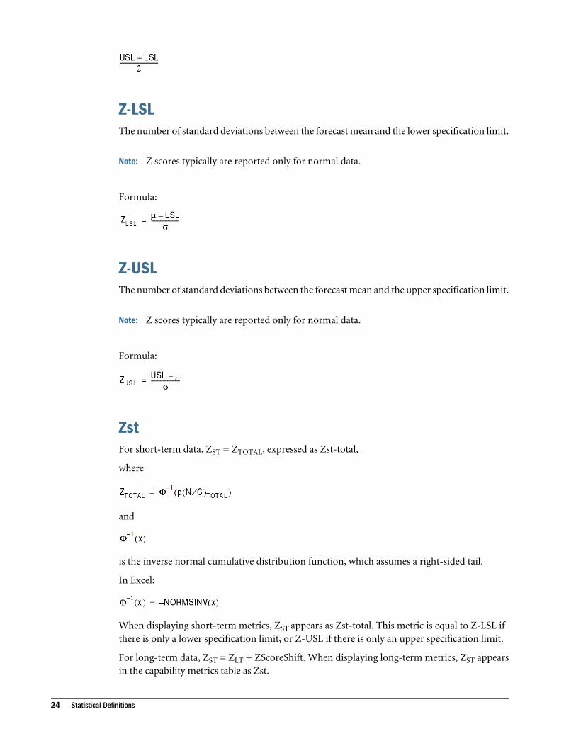
Z-LSLThe number of standard deviations between the forecast mean and the lower specification limit.
Note: Z scores typically are reported only for normal data.
Formula:
Z-USLThe number of standard deviations between the forecast mean and the upper specification limit.
Note: Z scores typically are reported only for normal data.
Formula:
ZstFor short-term data, ZST = ZTOTAL, expressed as Zst-total,
where
and
is the inverse normal cumulative distribution function, which assumes a right-sided tail.
In Excel:
When displaying short-term metrics, ZST appears as Zst-total. This metric is equal to Z-LSL ifthere is only a lower specification limit, or Z-USL if there is only an upper specification limit.
For long-term data, ZST = ZLT + ZScoreShift. When displaying long-term metrics, ZST appearsin the capability metrics table as Zst.
24 Statistical Definitions

Note: Z scores typically are reported only for normal data. The maximum value for Z scorescalculated by Crystal Ball from forecast data is 21.18.
Zst-totalFor short-term metrics when both specification limits are defined, the number of standarddeviations between the short-term forecast mean and the lower boundary of combining alldefects onto the upper tail of the normal curve. Also equal to Zlt-total plus the Z-score shiftvalue if long-term metrics are calculated.
When short-term metrics are calculated, Zst-total is equivalent to ZST, described in the previoussection.
Note: Z scores typically are reported only for normal data.
ZltFor long-term data, ZLT = ZTOTAL, expressed as Zlt-total,
where
ZTOTAL =
and
is the inverse normal cumulative distribution function, which assumes a right-sided tail.
In Excel:
When displaying long-term metrics, ZLT appears as Zlt-total. This metric is equal to Z-LSL ifthere is only a lower specification limit or Z-USL if there is only an upper specification limit.
For short-term data, ZLT = ZST - ZScoreShift. When displaying short-term metrics, ZLT appearsin the capability metrics table as Zlt.
Note: Z scores typically are reported only for normal data. The maximum value for Z scorescalculated by Crystal Ball from forecast data is 21.18.
Zlt-totalFor long-term metrics when both specification limits are defined, the number of standarddeviations between the long-term forecast mean and the lower boundary of combining all defects
Process Capability Metrics 25

onto the upper tail of the normal curve. Also equal to Zst-total minus the Z-score shift value ifshort-term metrics are calculated.
When long-term metrics are calculated, Zlt-total is equivalent to ZLT, described in the previoussection.
Note: Z scores typically are reported only for normal data.
p(N/C)-belowProbability of a defect below the lower specification limit; DPUBELOW .
Formula:
where F is the area beneath the normal curve below the LSL, otherwise known as unity minusthe normal cumulative distribution function for the LSL (assumes a right-sided tail).
In Excel:
p(N/C)-aboveProbability of a defect above the upper specification limit; DPUABOVE.
Formula:
where F is the area beneath the normal curve above the USL, otherwise known as unity minusthe normal cumulative distribution function for the USL (assumes a right-sided tail).
In Excel:
p(N/C)-totalProbability of a defect outside the lower and upper specification limits; DPUTOTAL.
Formula:
PPM-belowDefects below the lower specification limit, per million units.
26 Statistical Definitions
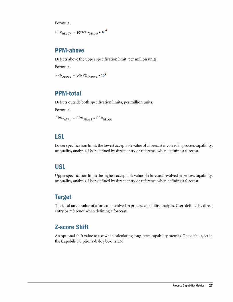
Formula:
PPM-aboveDefects above the upper specification limit, per million units.
Formula:
PPM-totalDefects outside both specification limits, per million units.
Formula:
LSLLower specification limit; the lowest acceptable value of a forecast involved in process capability,or quality, analysis. User-defined by direct entry or reference when defining a forecast.
USLUpper specification limit; the highest acceptable value of a forecast involved in process capability,or quality, analysis. User-defined by direct entry or reference when defining a forecast.
TargetThe ideal target value of a forecast involved in process capability analysis. User-defined by directentry or reference when defining a forecast.
Z-score ShiftAn optional shift value to use when calculating long-term capability metrics. The default, set inthe Capability Options dialog box, is 1.5.
Process Capability Metrics 27

28 Statistical Definitions

3Equations and Methods
In This Chapter
Introduction... . . . . . . . . . . . . . . . . . . . . . . . . . . . . . . . . . . . . . . . . . . . . . . . . . . . . . . . . . . . . . . . . . . . . . . . . . . . . . . . . . . . . . . . . . . . . . . . . . . . . . . . . . . . . . . . . . . . . . .29
Formulas for Probability Distributions ... . . . . . . . . . . . . . . . . . . . . . . . . . . . . . . . . . . . . . . . . . . . . . . . . . . . . . . . . . . . . . . . . . . . . . . . . . . . . . . . . . . . . . . . . .29
IntroductionThis chapter provides formulas for the probability distributions.
Formulas for other statistical terms are included in Chapter 2.
Formulas for Probability DistributionsThis section contains the formulas used to calculate probability distributions.
Beta DistributionParameters: Minimum value (Min), Maximum value (Max), Alpha (a), Beta (b)
Formula:
If 0 is less than x - Min is less than Max - Min, a is more than 0; b is more than 0
otherwise, 0
where:
where:
and where G is the Gamma function.
Method 1: Gamma Density Combination
Introduction 29

Comment: The Beta variate is obtained from:
where u = Gamma (a, 1) and v = Gamma (b, 1).
Method 2: Rational Fraction Approximation method with a Newton Polish step
Comment: This method is used instead of Method 1 when Latin Hypercube sampling is in effect.
BetaPERT DistributionParameters: Minimum value (Min), Most likely value (Likeliest), Maximum value (Max)
Formula:
for
where:
and is the beta integral.
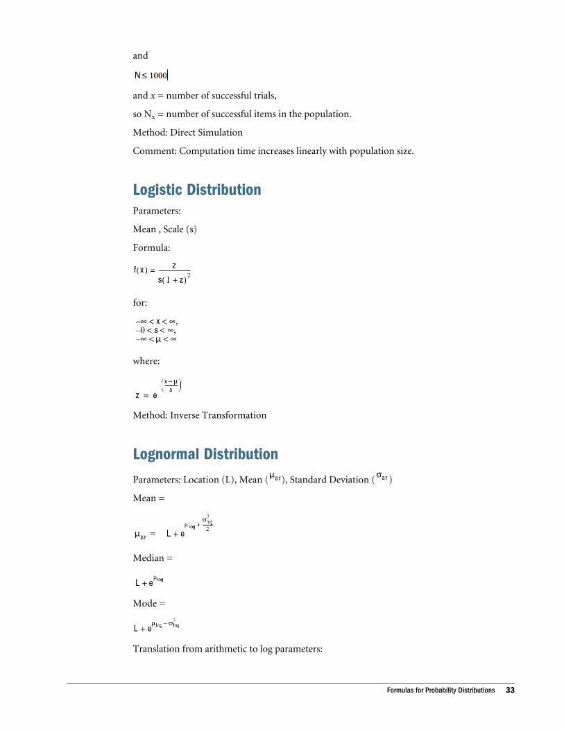
Binomial DistributionParameters: Probability of success (p), Number of total trials (n)
Formula:
for i = 0,1,2,...n; p is greater than 0; 0 is less than n is less than 1,000
where:
and x = number of successful trials
Method: Direct Simulation
Comment: Computation time increases linearly with number of trials.
30 Equations and Methods

Note: Crystal Ball limits n to 1,000, partly for performance reasons and partly because a binomialdistribution with a large n can be approximated with Poisson and normal distributions.The Poisson approximation should be used when n^0.31*(1-p) is less than 0.47, and thenormal approximation should be used when n^0.31*(1-p) is greater than 0.47.
Discrete Uniform DistributionParameters: Minimum value (Min), Maximum value (Max)
Formula:
Comment: This is the discrete equivalent of the uniform distribution, described in “ UniformDistribution” on page 38.
Exponential DistributionParameters: Success rate ( )
Formula:
Method: Inverse Transformation
Gamma DistributionThis distribution includes the Erlang and Chi-Square distributions as special cases.
Parameters: Location (L), Scale (s), Shape ( )
Formula:
where is the gamma function.
Note: Some textbook Gamma formulas use:
Formulas for Probability Distributions 31

Method 1:
When is less than 1, Vaduva’s rejection from a Weibull density.
When is greater than 1, Best’s rejection from a t density with 2 degrees of freedom.
When = 1, inverse transformation.
Method 2: Rational Fraction Approximation method with a Newton Polish step
Comment: This method is used instead of Method 1 when Latin Hypercube sampling is in effect.
Geometric DistributionParameters: Probability of success (p)
Formula:
for:
where x = number of successful trials
Method: Inverse Transformation
Hypergeometric DistributionParameters:
Number of successful items in the population (Nx), sampled trials (n), population size (N)
Formula:
where:
for:
32 Equations and Methods
and
and x = number of successful trials,
so Nx = number of successful items in the population.
Method: Direct Simulation
Comment: Computation time increases linearly with population size.
Logistic DistributionParameters:
Mean , Scale (s)
Formula:
for:
where:
Method: Inverse Transformation
Lognormal DistributionParameters: Location (L), Mean ( ), Standard Deviation ( )
Mean =
Median =
Mode =
Translation from arithmetic to log parameters:
Formulas for Probability Distributions 33

L = L; L is always in arithmetic space.
Log mean =
Log standard deviation =
where ln = natural logarithm.
Formula:
for:
Method: Inverse transformation
Translation from log to geometric parameters: L = L
Geometric mean =
Geometric std. dev. =
Translation from log to arithmetic parameters:
L = L
Arithmetic mean =
Arithmetic variance =
34 Equations and Methods

Maximum Extreme DistributionThe maximum extreme distribution is the positively skewed form of the extreme valuedistribution.
Parameters: Likeliest (m), Scale (s)
Formula:
for:
where:
Method: Inverse Transformation
Minimum Extreme DistributionThe minimum extreme distribution is the negatively skewed form of the extreme valuedistribution.
Parameters: Likeliest (m), Scale (s)
Formula:
for:
where:
Method: Inverse Transformation
Negative Binomial DistributionParameters: Probability of success (p), Shape ( )
Formula:
Formulas for Probability Distributions 35

where:
and x = total number of trials required
Method: Direct Simulation through summation of Geometric variates
Comment: Computation time increases linearly with Shape.
Mal DistributionThis distribution is also known as the Gaussian distribution.
Parameters:
Mean ( ), Standard Deviation ( )
Formula:
for:
Method 1: Polar Marsaglia
Comment: This method is somewhat slower than other methods, but its accuracy is essentiallyperfect.
Method 2: Rational Fraction Approximation
Comment: This method is used instead of the Polar Marsaglia method when Latin Hypercubesampling is in effect.
This method has a 7–8 digit accuracy over the central range of the distribution and a 5–6 digitaccuracy in the tails.
Pareto DistributionParameters:
Location (L), Shape ( )
Formula:
36 Equations and Methods

for:
is more than 0
Method: Inverse Transformation
Poisson DistributionParameters: Rate ( )
Formula:
Method: Direct Simulation through Summation of Exponential Variates
Comment: Computation time increases linearly with Rate.
Student’s t-DistributionParameters: Midpoint (m), Scale (s), Degrees of Freedom (d)
Formula:
where:
and where:
and where:
= the gamma function
Formulas for Probability Distributions 37

Triangular DistributionParameters: Minimum value (Min), Most likely value (Likeliest), Maximum value (Max)
Formula:
where:
Method: Inverse Transformation
Uniform DistributionParameters: Minimum value (Min), Maximum value (Max)
Formula:
Method: Multiplicative Congruential Generator
This routine uses the iteration formula:
Comment:
The generator has a period of length 231 - 2, or 2,147,483,646. This means that the cycle of randomnumbers repeats after several billion trials. This formula is discussed in detail in the SimulationModeling & Analysis and Art of Computer Programming, Vol. II, references in the Crystal BallUser's Guide bibliography.
Weibull DistributionA Weibull distribution with Shape = 2 is also known as the Rayleigh distribution.
Parameters:
Location (L), Scale (s), Shape ( )
Formula:
38 Equations and Methods
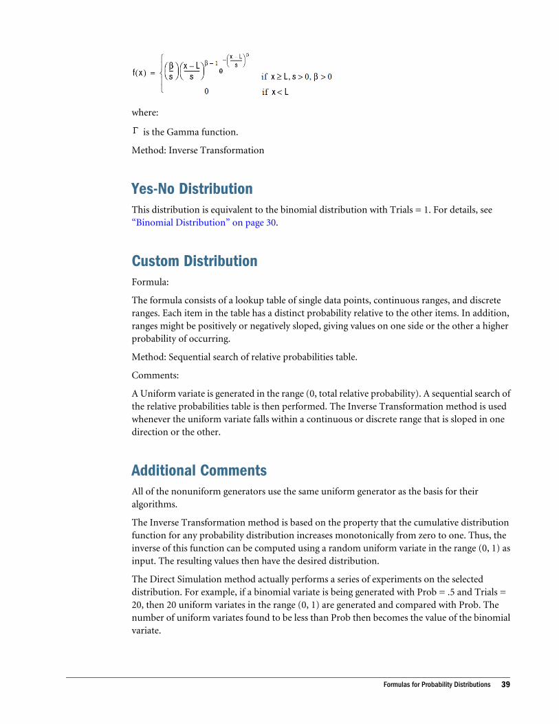
where:
is the Gamma function.
Method: Inverse Transformation
Yes-No DistributionThis distribution is equivalent to the binomial distribution with Trials = 1. For details, see“Binomial Distribution” on page 30.
Custom DistributionFormula:
The formula consists of a lookup table of single data points, continuous ranges, and discreteranges. Each item in the table has a distinct probability relative to the other items. In addition,ranges might be positively or negatively sloped, giving values on one side or the other a higherprobability of occurring.
Method: Sequential search of relative probabilities table.
Comments:
A Uniform variate is generated in the range (0, total relative probability). A sequential search ofthe relative probabilities table is then performed. The Inverse Transformation method is usedwhenever the uniform variate falls within a continuous or discrete range that is sloped in onedirection or the other.
Additional CommentsAll of the nonuniform generators use the same uniform generator as the basis for theiralgorithms.
The Inverse Transformation method is based on the property that the cumulative distributionfunction for any probability distribution increases monotonically from zero to one. Thus, theinverse of this function can be computed using a random uniform variate in the range (0, 1) asinput. The resulting values then have the desired distribution.
The Direct Simulation method actually performs a series of experiments on the selecteddistribution. For example, if a binomial variate is being generated with Prob = .5 and Trials =20, then 20 uniform variates in the range (0, 1) are generated and compared with Prob. Thenumber of uniform variates found to be less than Prob then becomes the value of the binomialvariate.
Formulas for Probability Distributions 39

Distribution Fitting MethodsDuring distribution fitting, Crystal Ball computes Maximum Likelihood Estimators (MLEs) tofit most of the probability distributions to a data set. In effect, this method chooses values forthe parameters of the distributions that maximize the probability of producing the actual dataset. Sometimes, however, the MLEs do not exist for some distributions (for example, gamma,beta). In these cases, Crystal Ball resorts to other natural parameter estimation techniques.
When the MLEs do exist, they exhibit desirable properties:
l They are minimum-variance estimators of the parameters.
l As the data set grows, the biases in the MLEs tend to zero.
For several of the distributions (for example, uniform, exponential), it is possible to remove thebiases after computing the MLEs to yield minimum-variance unbiased estimators (MVUEs) ofthe distribution parameters. These MVUEs are the best possible estimators.
40 Equations and Methods

4Default Names and Distribution
Parameters
In This Chapter
Introduction... . . . . . . . . . . . . . . . . . . . . . . . . . . . . . . . . . . . . . . . . . . . . . . . . . . . . . . . . . . . . . . . . . . . . . . . . . . . . . . . . . . . . . . . . . . . . . . . . . . . . . . . . . . . . . . . . . . . . . .41
Naming Defaults .. . . . . . . . . . . . . . . . . . . . . . . . . . . . . . . . . . . . . . . . . . . . . . . . . . . . . . . . . . . . . . . . . . . . . . . . . . . . . . . . . . . . . . . . . . . . . . . . . . . . . . . . . . . . . . . . . .41
Distribution Parameter Defaults .. . . . . . . . . . . . . . . . . . . . . . . . . . . . . . . . . . . . . . . . . . . . . . . . . . . . . . . . . . . . . . . . . . . . . . . . . . . . . . . . . . . . . . . . . . . . . . . . .41
IntroductionThis first section of this chapter describes the process Crystal Ball uses to name assumptions,decision variables, and forecasts. The second section shows the values it assigns to each of thedistribution types.
Naming DefaultsWhen defining an assumption, decision variable, or forecast, Crystal Ball uses the followingsequence to generate a default name for the data cell:
1. Checks for a range name and, if found, uses it as the cell name.
2. Checks the cell immediately to the left of the selected cell. If it is a text cell, Crystal Ball usesthat text as the cell name.
3. Checks the cell immediately above the selected cell. If it is a text cell, Crystal Ball uses thattext as the cell name.
4. If there is no applicable text or range name, Crystal Ball uses the cell coordinates for thename (for example, B3 or C7).
Distribution Parameter DefaultsThis section lists the initial values Crystal Ball provides for the primary parameters in the DefineAssumption dialog:
l “Beta” on page 42
l “BetaPERT” on page 43
l “Binomial” on page 43
l “Custom” on page 43
Introduction 41

l “Discrete Uniform” on page 43
l “Exponential” on page 44
l “Gamma” on page 44
l “Geometric” on page 44
l “Hypergeometric” on page 44
l “Logistic” on page 45
l “Lognormal” on page 45
l “Maximum Extreme Value” on page 45
l “Minimum Extreme Value” on page 45
l “Negative Binomial” on page 46
l “Normal” on page 46
l “Pareto” on page 46
l “Poisson” on page 47
l “Student’s t” on page 47
l “Triangular” on page 47
l “Uniform” on page 47
l “Weibull” on page 48
l “Yes-No” on page 48
If an alternate parameter set is selected as the default mode, the primary parameters are stillcalculated as described below before conversion to the alternate parameters.
Note: Extreme values on the order of 1e±9 or ±1e16 may yield results somewhat different fromthose listed here.
BetaIf the cell value is 0:
Minimum is -10.00
Maximum is 10.00
Alpha is 2
Beta is 3
Otherwise:
Minimum is cell value - (absolute cell value divided by 10)
Maximum is cell value + (absolute cell value divided by 10)
Alpha is 2
Beta is 3
42 Default Names and Distribution Parameters

For out-of-range values, such as ±1e300:
Minimum is 0
Maximum is 1
Alpha is 2
Beta is 3
BetaPERTIf the cell value is 0:
Likeliest is 0
Minimum is -10.00
Maximum is 10.00
Otherwise:
Likeliest is cell value
Minimum is cell value - (absolute cell value divided by 10)
Maximum is cell value + (absolute cell value divided by 10)
BinomialIf the cell value is between 0 and 1:
Probability is the cell value
Trials is 50
If the cell value is between 1 and 1,000 (the maximum number of binomial trials):
Probability (Prob) is 0.5
Trials is cell value
Otherwise:
Probability (Prob) is 0.5
Trials is 50
CustomInitially empty.
Discrete UniformIf the cell value is 0 or -1e9:
Distribution Parameter Defaults 43

Minimum is 0
Maximum is 10
Otherwise:
Minimum is cell value - INT (absolute cell value divided by 10)
Maximum is cell value + INT (absolute cell value divided by 10)
ExponentialIf the cell value is 0, rate is 1.0.
Otherwise, rate is 1 divided by the absolute cell value.
GammaIf the cell value is 0:
Location is 0.00
Scale is 1.00
Shape is 2
Otherwise:
Location is cell value
Scale is absolute cell value divided by 10
Shape is 2
GeometricIf the cell value is greater than 0 and less than 1, probability is cell value.
Otherwise, probability is 0.2.
HypergeometricIf the cell value is greater than 0 and less than 1:
Success is 100 times cell value
Trials is 50
Population size is 100
If the cell value is between 2 and the maximum number of Hypergeometric trials (1,000):
Success is cell value divided by 2 (rounded downward)
Trials is cell value divided by 2 (rounded downward)
44 Default Names and Distribution Parameters

Population size is cell value
Otherwise:
Sucess is 50
Trials is 50
Population size is 100
LogisticIf the cell value is 0:
Mean is 0
Scale is 1.0.
Otherwise:
Mean is cell value
Scale is absolute cell value divided by 10
LognormalIf the cell value is greater than 0:
Mean is cell value
Standard deviation is absolute cell value divided by 10
Otherwise:
Mean is e
Standard deviation is 1.0
Maximum Extreme ValueIf the cell value is 0:
Likeliest is 0
Scale is 1
Otherwise:
Likeliest is cell value
Scale is absolute cell value divided by 10
Minimum Extreme ValueIf the cell value is 0:
Distribution Parameter Defaults 45

Likeliest is 0
Scale is 1
Otherwise:
Likeliest is cell value
Scale is absolute cell value divided by 10
Negative BinomialIf the cell value is less than or equal to 0:
Probability is 0.2
Shape is 10
If the cell value is greater than 0 and less than 1:
Probability is cell value
Shape is 10
Otherwise, unless the cell value is greater than 100:
Probability is 0.2
Shape is cell value
If the cell value is greater than 100, the shape is 10.
NormalIf the cell value is 0:
Mean is 0
Standard deviation is 1.00
Otherwise, unless the cell value is more than 100:
Mean is cell value
Standard deviation is absolute cell value divided by 10.0
ParetoIf the cell value is between 1.0 and 1,000:
Location is cell value
Shape is 2
Otherwise:
Location is 1.00
46 Default Names and Distribution Parameters

Shape is 2
PoissonIf the cell value is less than or equal to 0, the rate is 10.00.
If the cell value is greater than 0 and less than or equal to the maximum rate (1,000), the rate isthe cell value.
Otherwise, the rate is 10.00
Student’s tIf the cell value is 0:
Midpoint is 0
Scale is 1.00
Degrees is 5
Otherwise:
Midpoint is cell value
Scale is absolute cell value divided by 10
Degrees is 5
TriangularIf the cell value is 0:
Likeliest is 0
Minimum is -10.00
Maximum is 10.00
Otherwise:
Likeliest is cell value
Minimum is cell value minus absolute cell value divided by 10
Maximum is cell value plus absolute cell value divided by 10
UniformIf the cell value is 0:
Minimum is -10.00
Maximum is 10.00
Distribution Parameter Defaults 47

Otherwise:
Minimum is cell value minus absolute cell value divided by 10.0
Maximum is cell value plus absolute cell value divided by 10.0
WeibullIf the cell value is 0:
Location is 0
Scale is 1.00
Shape is 2
Otherwise:
Location is cell value
Scale is absolute cell value divided by 10
Shape is 2
Yes-NoIf the cell value is greater than 0 and less than 1, the probability of Yes(1) equals the cell value.
Otherwise, the probability of Yes(1) equals 0.5.
48 Default Names and Distribution Parameters

5Predictor Formulas and
Statistics
In This Chapter
Introduction... . . . . . . . . . . . . . . . . . . . . . . . . . . . . . . . . . . . . . . . . . . . . . . . . . . . . . . . . . . . . . . . . . . . . . . . . . . . . . . . . . . . . . . . . . . . . . . . . . . . . . . . . . . . . . . . . . . . . . .49
Time-Series Forecasting Techniques ... . . . . . . . . . . . . . . . . . . . . . . . . . . . . . . . . . . . . . . . . . . . . . . . . . . . . . . . . . . . . . . . . . . . . . . . . . . . . . . . . . . . . . . . . . .49
Time-Series Forecasting Method Formulas ... . . . . . . . . . . . . . . . . . . . . . . . . . . . . . . . . . . . . . . . . . . . . . . . . . . . . . . . . . . . . . . . . . . . . . . . . . . . . . . . . . . .52
Error Measure and Statistic Formulas... . . . . . . . . . . . . . . . . . . . . . . . . . . . . . . . . . . . . . . . . . . . . . . . . . . . . . . . . . . . . . . . . . . . . . . . . . . . . . . . . . . . . . . . . .56
Regression Methods ... . . . . . . . . . . . . . . . . . . . . . . . . . . . . . . . . . . . . . . . . . . . . . . . . . . . . . . . . . . . . . . . . . . . . . . . . . . . . . . . . . . . . . . . . . . . . . . . . . . . . . . . . . . . .62
Regression Statistic Formulas ... . . . . . . . . . . . . . . . . . . . . . . . . . . . . . . . . . . . . . . . . . . . . . . . . . . . . . . . . . . . . . . . . . . . . . . . . . . . . . . . . . . . . . . . . . . . . . . . . .64
IntroductionThis chapter provides formulas and techniques used in Predictor. It contains these main topics:
l “Time-Series Forecasting Techniques” on page 49
l “Time-Series Forecasting Method Formulas” on page 52
l “Error Measure and Statistic Formulas” on page 56
l “Regression Methods” on page 62
l “Regression Statistic Formulas” on page 64
Time-Series Forecasting TechniquesThis section discusses statistics related to time-series forecasting techniques available inPredictor:
l “Standard Forecasting” on page 50
l “Holdout Forecasting” on page 50
l “Simple Lead Forecasting” on page 51
l “Weighted Lead Forecasting” on page 51
Related terms:
l Time series—The original data, expressed as Yt
l Fit array—A retrofit of the time series, consisting of one-period-ahead forecasts performedfrom the data of previous periods; expressed as Ft
Introduction 49

l Residual array—A set of positive or negative residuals, expressed as rt, and defined as rt =Yt – Ft
l RMSE—Root mean square error for forecasting, calculated as described in “RMSE” on page57, where n is the number of periods for which a fit is available. RMSE depends on thespecific forecasting method and technique.
l Forecasts—Value projections calculated using the formula for the specific method; they are1 to k periods ahead, where k is the number of forecasts required
l Standard error of forecasts—Used to calculate confidence intervals; see “ConfidenceIntervals” on page 58
Standard ForecastingIn standard forecasting, if the method parameters are already provided by the user, the followingare calculated: RMSE and other error measures, forecasts, and standard error. If the parametersare not provided by the user, then the parameters are optimized to minimize the error measurebetween the fit values and the historical data for the same period.
Holdout ForecastingIn holdout forecasting:
l The last few data points are removed from the data series. The remaining historical dataseries is called in-sample data, and the holdout data is called out-of-sample data. Supposep periods have been removed as holdout from a total of N periods.
l Parameters are optimized by minimizing the fit error measure for in-sample data. If methodparameters are provided by the user, those are used in the final forecasting.
l After the parameters are optimized, the forecasts for the holdout periods (p periods) arecalculated.
l The error statistics (RMSE, MAD, MAPE) are out-of-sample statistics, based on only thenumbers in the hold-out period. The RMSE for holdout forecasting is often called holdoutRMSE. The holdout error measures are the ones reported to the user and are used to sortthe forecasting methods.
l Other statistics such as Theil's U, Durbin-Watson, and Ljung-Box are in-sample statistics,based on the non-holdout period.
l Final forecasting is performed on both the in-sample and out-of-sample periods (all Nperiods) using the standard technique.
l The standard error for the forecasts is also calculated using all N periods.
To improve the optimized parameter values obtained for the method, holdout forecasting shouldbe used only when there are at least 100 data points for non-seasonal methods and 5 seasons forseasonal methods. For best results, use no more than 5 percent of the data points as holdout, nomatter how large the number of total data points.
50 Predictor Formulas and Statistics
Simple Lead ForecastingSimple lead forecasting optimizes the forecasting parameters to minimize the error measurebetween the historical data and the fit values, both offset by a specified number of periods (lead).Use this forecasting technique when a forecast for some future time period has more importancethan forecasts for previous or later periods.
For example, suppose a company must order extremely expensive manufacturing componentstwo months in advance, making the forecast for two months out the most important. In thiscase, the company could use simple lead forecasting with a lead of 2 periods.
In simple lead forecasting:
l The fit for period t is calculated as the (lead)-period-ahead forecast from period t = 0. Thefit for t = 1 calculated with simple lead forecasting is the same as the fit for the standardforecast, which is a 1-period-ahead forecast from period t = 0.
l The residual at period t is calculated as the difference between the historical value at periodt and the lead-period-fit obtained for period (t).
l The lead RMSE is calculated as the root mean square of the residuals as calculated above.
l The forecasts for future periods and the standard errors for those forecasts are calculated asfor standard forecasts.
If the method parameters are already provided by the user, simple lead forecasting is performedas described previously. If the parameters are not provided, then the parameters are optimizedto minimize the lead error measure (for example, lead RMSE). After the parameters areoptimized, the fit and the forecast are then calculated as for standard forecasting method.
Weighted Lead ForecastingWeighted lead forecasting optimizes the forecasting parameters to minimize the average errormeasure between the historical data and the fit values, offset by 1, 2, and so on, up to the specifiednumber of periods (lead value). It uses the simple lead technique for several lead periods, averagesthe error measure over the periods, and then optimizes this average value to obtain the methodparameters.
Use weighted lead forecasting when the future forecast for several periods is most important.For example, suppose your company must order extremely expensive manufacturingcomponents one and two months in advance, making forecasts for all the time periods up totwo months out the most important.
In weighted lead forecasting:
l Simple lead error measures are calculated for lead values from 1 to the specified lead value.
l The weighted lead RMSE is calculated as the average of the simple lead RMSEs starting fromlead value = 1 to the specified lead value period. For a lead value of 3, simple lead errormeasures for 1, 2, and 3 are obtained and then averaged to get the weighted lead RMSE.
l Method parameters are then obtained by minimizing the weighted lead RMSE.
Time-Series Forecasting Techniques 51

l After the parameters are obtained, forecasts for future periods and the standard errors forthose forecasts are calculated as for standard forecasts.
If method parameters are provided by the user, weighted lead forecasting is performed asdescribed previously. If the parameters are not provided, they are optimized to minimize theweighted lead error measure, such as weighted lead RMSE.
After parameters are optimized, the fit and the forecast are then calculated as for the standardforecasting method. For a lead value = 1, weighted lead forecasting is the same as simple leadforecasting and standard forecasting.
Time-Series Forecasting Method FormulasThis section provides formulas for the following time-series forecasting methods used in CBPredictor:
l “Nonseasonal Forecasting Method Formulas” on page 52
l “Seasonal Forecasting Method Formulas” on page 53
Nonseasonal Forecasting Method FormulasFormulas for the nonseasonal time-series forecasting methods:
l “Single Moving Average” on page 52
l “Double Moving Average” on page 52
l “Single Exponential Smoothing” on page 53
l “Double Exponential Smoothing” on page 53
Single Moving AverageSingle moving average formulas:
(Fit)
(Forecast for period m) Ft+m = Ft
where the parameterse are:
p—Order of moving average
Note: First fit is available from period (p + 1)
Double Moving AveragePredictor uses the following equations for the double moving average method:
52 Predictor Formulas and Statistics
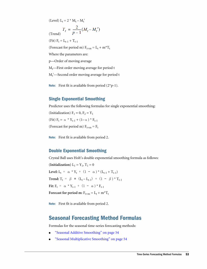
(Level) Lt = 2 * Mt – Mt'
(Trend)
(Fit) Ft = Lt-1 + Tt-1
(Forecast for period m) Ft+m = Lt + m*Tt
Where the parameters are:
p—Order of moving average
Mt—First order moving average for period t
Mt'—Second order moving average for period t
Note: First fit is available from period (2*p-1).
Single Exponential SmoothingPredictor uses the following formulas for single exponential smoothing:
(Initialization) F1 = 0, F2 = Y1
(Fit) Ft = α * Yt-1 + (1–α) * Ft-1
(Forecast for period m) Ft+m = Ft
Note: First fit is available from period 2.
Double Exponential SmoothingCrystal Ball uses Holt’s double exponential smoothing formula as follows:
(Initialization) L1 = Y1, T1 = 0
Level: Lt = α * Yt + (1 – α) * (Lt-1 + Tt-1)
Trend: Tt = β * (Lt – Lt-1) + (1 – β) * Tt-1
Fit: Ft = α * Yt-1 + (1 – α) * Ft-1
Forecast for period m: Ft+m = Lt + m*Tt
Note: First fit is available from period 2.
Seasonal Forecasting Method FormulasFormulas for the seasonal time-series forecasting methods:
l “Seasonal Additive Smoothing” on page 54
l “Seasonal Multiplicative Smoothing” on page 54
Time-Series Forecasting Method Formulas 53

l “Holt-Winters’ Additive Seasonal Smoothing” on page 55
l “Holt-Winters’ Multiplicative Seasonal Smoothing” on page 56
Seasonal Additive SmoothingCrystal Ball uses the following initialization equation for this method:
Set Lt = P, St = Yt – P for t = 1 to s
Crystal Ball uses the following equations to calculate this method:
where the parameters are:
α—Alpha
γ—Gamma
m—Number of periods ahead to forecast
s—Length of seasonality
Lt—Level of the series at time t
St—Seasonal component at time t
Note: First fit is available from period (s + 1)
Seasonal Multiplicative SmoothingCrystal Ball uses the following initialization equation for this method:
Set Lt = P, St = Yt/P for t = 1 to s
Crystal Ball uses the following equations to calculate this method:
54 Predictor Formulas and Statistics
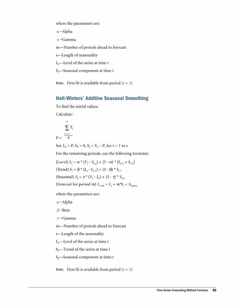
where the parameters are:
α—Alpha
γ—Gamma
m—Number of periods ahead to forecast
s—Length of seasonality
Lt—Level of the series at time t
St—Seasonal component at time t
Note: First fit is available from period (s + 1)
Holt-Winters’ Additive Seasonal SmoothingTo find the initial values:
Calculate:
P =
Set: Lt = P, bt = 0, St = Yt – P, for t = 1 to s
For the remaining periods, use the following formulas:
where the parameters are:
α—Alpha
β—Beta
γ—Gamma
m—Number of periods ahead to forecast
s—Length of the seasonality
Lt—Level of the series at time t
bt—Trend of the series at time t
St—Seasonal component at time t
Note: First fit is available from period (s + 1)
Time-Series Forecasting Method Formulas 55
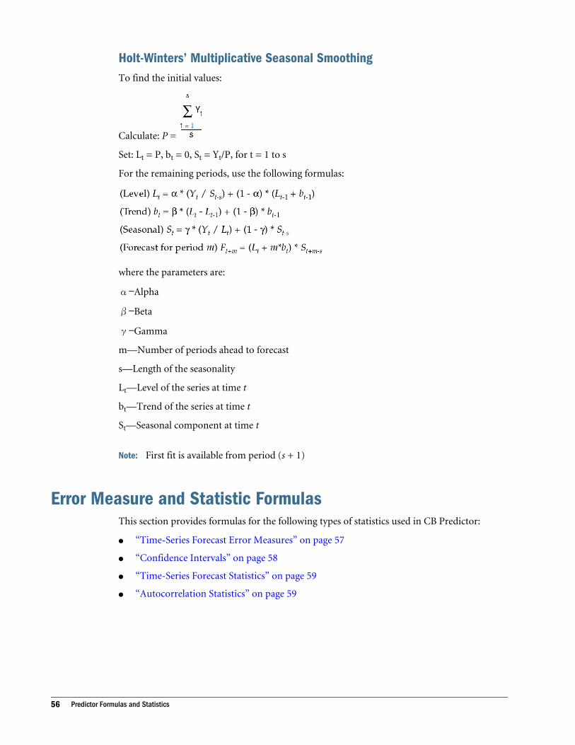
Holt-Winters’ Multiplicative Seasonal SmoothingTo find the initial values:
Calculate: P =
Set: Lt = P, bt = 0, St = Yt/P, for t = 1 to s
For the remaining periods, use the following formulas:
where the parameters are:
α—Alpha
β—Beta
γ—Gamma
m—Number of periods ahead to forecast
s—Length of the seasonality
Lt—Level of the series at time t
bt—Trend of the series at time t
St—Seasonal component at time t
Note: First fit is available from period (s + 1)
Error Measure and Statistic FormulasThis section provides formulas for the following types of statistics used in CB Predictor:
l “Time-Series Forecast Error Measures” on page 57
l “Confidence Intervals” on page 58
l “Time-Series Forecast Statistics” on page 59
l “Autocorrelation Statistics” on page 59
56 Predictor Formulas and Statistics

Time-Series Forecast Error MeasuresCrystal Ball calculates three different error measures for the fit of each time-series forecast.Crystal Ball uses one of these error measures to determine which time-series forecasting methodis the best:
l “RMSE” on page 57
l “MAD” on page 57
l “MAPE” on page 58
RMSERoot mean squared error is an absolute error measure that squares the deviations to keep thepositive and negative deviations from canceling one another out. This measure also tends toexaggerate large errors, which can help when comparing methods.
The formula for calculating RMSE:
where Yt is the actual value of a point for a given time period t, n is the total number of fittedpoints, and
is the fitted forecast value for the time period t.
MADMean absolute deviation is an error statistic that averages the distance between each pair of actualand fitted data points.
The formula for calculating the MAD:
where Yt is the actual value of a point for a given time period t, n is the total number of fittedpoints, and
is the forecast value for the time period t.
Error Measure and Statistic Formulas 57

MAPEMean absolute percentage error is a relative error measure that uses absolute values to keep thepositive and negative errors from canceling one another out and uses relative errors to enableyou to compare forecast accuracy between time-series models.
The formula for calculating the MAPE:
where Yt is the actual value of a point for a given time period t, n is the total number of fittedpoints, and
is the forecast value for the time period t.
Note: If Yt equals zero, Crystal Ball drops the term:
Confidence IntervalsThe confidence interval defines the range within which a forecasted value has some probabilityof occurring. Predictor uses an empirical method of calculating confidence intervals, using thestandard error of forecasts:
l For an m-period-ahead forecast, the error term rt(m) is defined as Yt – Ft(m), where Ft(m)is the m-period-ahead fit for period t.
l The standard error of prediction for an m-period-ahead forecast is then expressed as
where n is the number of periods for which rt(m) is defined.
Assuming that forecast errors are normally distributed, the formula for predicting the futurevalue of
at time t within a 95 percent confidence interval is
The empirical method is reasonably accurate when historical data amount is sufficiently large.
58 Predictor Formulas and Statistics

Time-Series Forecast StatisticsAnother statistic calculated for any time-series forecast is Theil’s U.
Theil’s U StatisticThis statistic compares forecasted results with the results of forecasting with minimal historicaldata.
The formula for calculating Theil’s U statistic:
where Yt is the actual value of a point for a given time period t, n is the number of data points,and
is the forecasted value.
Autocorrelation StatisticsMeasures of autocorrelation describe the relationship among values of the same data series atdifferent time periods.
The number of autocorrelations calculated is equal to the effective length of the time seriesdivided by 2, where the effective length of a time series is the number of data points in the serieswithout the pre-data gaps. The number of autocorrelations calculated ranges between aminimum of 2 and a maximum of 400.
Autocorrelation formula:
where rk is the autocorrelation for lag k.
Related statistics:
l “Autocorrelation Probability” on page 60
l “Durbin-Watson Statistic” on page 60
l “Ljung-Box Statistic” on page 61
Error Measure and Statistic Formulas 59

Autocorrelation and these statistics can be used to calculate seasonality as described in“Calculating Seasonality with Autocorrelations” on page 61.
Autocorrelation ProbabilityAutocorrelation probability is the probability of obtaining a certain autocorrelation for aparticular data series by chance alone, if the data were completely random. To calculateautocorrelation probability:
l Calculate the standard error of autocorrelation:
where
SE(rk) = standard error of autocorrelation at lag k
ri = autocorrelation at lag i
k = the time lag
n = number of observations in the time series
Reference: Hanke et al. Business Forecasting. 7th ed. Prentice Hall, 2001. Chapter 3, pg 59–60
l Calculate the t statistic:
l Calculate the p-value from the absolute t statistic; the probability is double the area of (1 –CDF(t))
Durbin-Watson StatisticThe Durbin-Watson statistic calculates autocorrelation at lag 1.
The formula for calculating the Durbin-Watson statistic:
where et is the difference between the estimated point
and the actual point (Yi) and n is the number of data points.
60 Predictor Formulas and Statistics
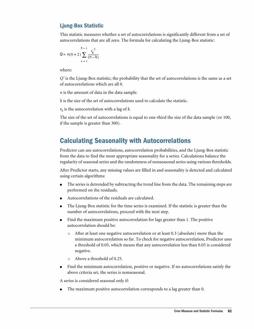
Ljung-Box StatisticThis statistic measures whether a set of autocorrelations is significantly different from a set ofautocorrelations that are all zero. The formula for calculating the Ljung-Box statistic:
where:
Q’ is the Ljung-Box statistic; the probability that the set of autocorrelations is the same as a setof autocorrelations which are all 0.
n is the amount of data in the data sample.
h is the size of the set of autocorrelations used to calculate the statistic.
rk is the autocorrelation with a lag of k.
The size of the set of autocorrelations is equal to one-third the size of the data sample (or 100,if the sample is greater than 300).
Calculating Seasonality with AutocorrelationsPredictor can use autocorrelations, autocorrelation probabilities, and the Ljung-Box statisticfrom the data to find the most appropriate seasonality for a series. Calculations balance theregularity of seasonal series and the randomness of nonseasonal series using various thresholds.
After Predictor starts, any missing values are filled in and seasonality is detected and calculatedusing certain algorithms:
l The series is detrended by subtracting the trend line from the data. The remaining steps areperformed on the residuals.
l Autocorrelations of the residuals are calculated.
l The Ljung-Box statistic for the time series is examined. If the statistic is greater than thenumber of autocorrelations, proceed with the next step.
l Find the maximum positive autocorrelation for lags greater than 1. The positiveautocorrelation should be:
m After at least one negative autocorrelation or at least 0.3 (absolute) more than theminimum autocorrelation so far. To check for negative autocorrelation, Predictor usesa threshold of 0.05, which means that any autocorrelation less than 0.05 is considerednegative.
m Above a threshold of 0.25.
l Find the minimum autocorrelation, positive or negative. If no autocorrelations satisfy theabove criteria set, the series is nonseasonal.
A series is considered seasonal only if:
l The maximum positive autocorrelation corresponds to a lag greater than 0.
Error Measure and Statistic Formulas 61
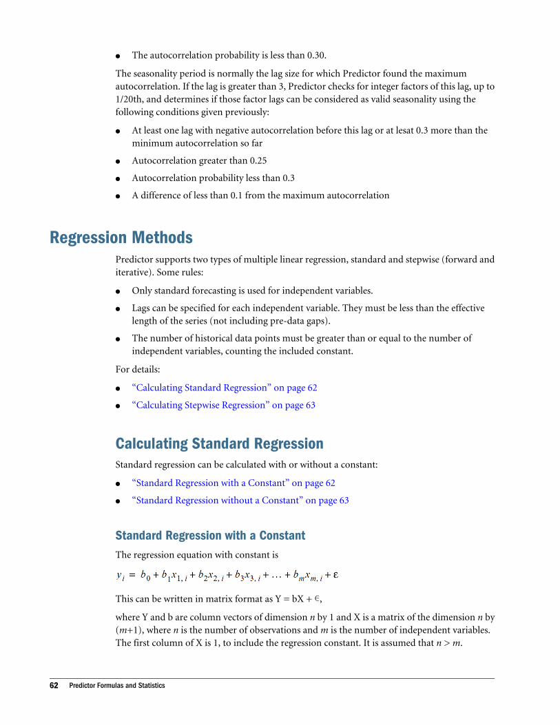
l The autocorrelation probability is less than 0.30.
The seasonality period is normally the lag size for which Predictor found the maximumautocorrelation. If the lag is greater than 3, Predictor checks for integer factors of this lag, up to1/20th, and determines if those factor lags can be considered as valid seasonality using thefollowing conditions given previously:
l At least one lag with negative autocorrelation before this lag or at lesat 0.3 more than theminimum autocorrelation so far
l Autocorrelation greater than 0.25
l Autocorrelation probability less than 0.3
l A difference of less than 0.1 from the maximum autocorrelation
Regression MethodsPredictor supports two types of multiple linear regression, standard and stepwise (forward anditerative). Some rules:
l Only standard forecasting is used for independent variables.
l Lags can be specified for each independent variable. They must be less than the effectivelength of the series (not including pre-data gaps).
l The number of historical data points must be greater than or equal to the number ofindependent variables, counting the included constant.
For details:
l “Calculating Standard Regression” on page 62
l “Calculating Stepwise Regression” on page 63
Calculating Standard RegressionStandard regression can be calculated with or without a constant:
l “Standard Regression with a Constant” on page 62
l “Standard Regression without a Constant” on page 63
Standard Regression with a ConstantThe regression equation with constant is
This can be written in matrix format as Y = bX + ∊,
where Y and b are column vectors of dimension n by 1 and X is a matrix of the dimension n by(m+1), where n is the number of observations and m is the number of independent variables.The first column of X is 1, to include the regression constant. It is assumed that n > m.
62 Predictor Formulas and Statistics

Predictor uses singular value decomposition (SVD) to determine the coefficients of a regressionequation. The primary difference between the singular value decomposition and the least squarestechniques is that the singular value decomposition technique can handle situations where theequations used to determine the coefficients of the regression equation are singular or close tosingular, which happens when performing regression on equations that represent parallel linesor surfaces. In these cases, the least squares technique returns no solution for the singular caseand extremely large parameters for the close-to-singular case.
Crystal Ball uses the matrix technique for singular value decomposition. Starting with:
y = bX
Following SVD, X can be rewritten:
X = [U][w][V]
where U, w, and V are the factor matrices. The matrix w, a square matrix of dimension (m+1)by (m+1), is a diagonal matrix with the singular values (or eigenvalues). U and V are other factormatrices..
The coefficients can then be calculated. For example, the b matrix is b = [V][w]-1[UT][y]
The fit vector ( ) is then calculated as = bX
For related regression statistics, see “Statistics, Standard Regression with Constant” on page64.
Standard Regression without a ConstantThis case is also known as regression through origin.
The regression equation without constant is
This can be written in matrix format as Y = bX + ∊, where Y and b are column vectors ofdimension n by 1 and X is a matrix of the dimension n by m, where n is the number of observationsand m is the number of independent variables. It is assumed that n > m.
Here, too, Predictor uses singular value decomposition (SVD) to determine b, the coefficientsof the regression equation. The only difference between this case and regression with a constantis the dimension of the matrices.
For related regression statistics, see “Statistics, Standard Regression without Constant” on page66.
Calculating Stepwise RegressionStepwise regression is described in Appendix C of the Crystal Ball Predictor User's Guide. Notethat the partial F statistic is only used in calculating stepwise regression. For a discussion, see“Statistics, Stepwise Regression” on page 68.
Regression Methods 63

Regression Statistic FormulasThe statistics used to analyze a regression are different from those used to analyze a time-seriesforecast. Regression statistics:
l “Statistics, Standard Regression with Constant” on page 64
l “Statistics, Standard Regression without Constant” on page 66
l “Statistics, Stepwise Regression” on page 68
Statistics, Standard Regression with ConstantThese statistics describe a standard regression including the constant:
l “ANOVA” on page 64
l “R2” on page 64
l “Adjusted R2” on page 65
l “SSE” on page 65
l “F” on page 65
l “Statistics for Individual Coefficients” on page 65
ANOVAANOVA (analysis of variance) statistics for standard regression with a constant:
Table 1 ANOVA Statistics, Standard Regression with a Constant
Source Sum of Squares Degrees of Freedom Mean Square F Ratio
Regression m MSR = SSR/m
Error n – m – 1 MSE = SSE/(n – m– 1)
Total n – 1 n/a n/a
The F statistic follows an F distribution with (m, n – m – 1) degrees of freedom. This informationis used to calculate the p-value of the F statistic.
R2
R2 is the coefficient of determination. This statistic represents the proportion of error for whichthe regression accounts.
64 Predictor Formulas and Statistics

You can use many methods to calculate R2. Predictor uses the equation:
Adjusted R2
You can calculate a regression equation by using the same number of data points as you haveequation coefficients. However, the regression equation will not be as universal as a regressionequation calculated using three times the number of data points as equation coefficients.
To correct the R2 for such situations, an adjusted R2 takes into account the degrees of freedomof an equation. When you suspect that an R2 is higher than it should be, calculate the R2 andadjusted R2. If the R2 and the adjusted R2 are close, then the R2 is probably accurate. If R2 ismuch higher than the adjusted R2, you probably do not have enough data points to calculatethe regression accurately.
The formula for adjusted R2:
Adjusted R2 =
where n is the number of data points and m is the number of independent variables.
SSESSE (standard error of measurement) is a measure of the amount the actual values differ fromthe fitted values. The formula for SSE:
where n is the number of data points you have and m is the number of independent variables.
FThe F statistic checks the significance of the relationship between the dependent variable andthe particular combination of independent variables in the regression equation. The F statisticis based on the scale of the Y values, so analyze this statistic in combination with the p–value(described in the next section). When comparing the F statistics for similar sets of data with thesame scale, the higher F statistic is better.
The formula for the F statistic is given in Table 1 on page 64.
Statistics for Individual CoefficientsFollowing are the statistics for the pth coefficient, including the regression constant:
Regression Statistic Formulas 65
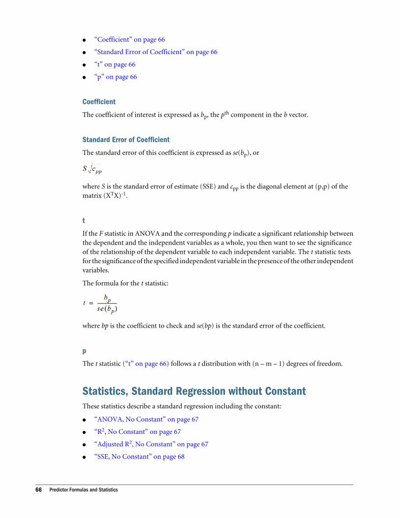
l “Coefficient” on page 66
l “Standard Error of Coefficient” on page 66
l “t” on page 66
l “p” on page 66
Coefficient
The coefficient of interest is expressed as bp, the pth component in the b vector.
Standard Error of Coefficient
The standard error of this coefficient is expressed as se(bp), or
where S is the standard error of estimate (SSE) and cpp is the diagonal element at (p,p) of thematrix (XTX)-1.
t
If the F statistic in ANOVA and the corresponding p indicate a significant relationship betweenthe dependent and the independent variables as a whole, you then want to see the significanceof the relationship of the dependent variable to each independent variable. The t statistic testsfor the significance of the specified independent variable in the presence of the other independentvariables.
The formula for the t statistic:
where bp is the coefficient to check and se(bp) is the standard error of the coefficient.
p
The t statistic (“t” on page 66) follows a t distribution with (n – m – 1) degrees of freedom.
Statistics, Standard Regression without ConstantThese statistics describe a standard regression including the constant:
l “ANOVA, No Constant” on page 67
l “R2, No Constant” on page 67
l “Adjusted R2, No Constant” on page 67
l “SSE, No Constant” on page 68
66 Predictor Formulas and Statistics

l “F, No Constant” on page 68
l “Statistics for Individual Coefficients, No Constant” on page 68
ANOVA, No ConstantANOVA (analysis of variance) statistics for standard regression with a constant:
Table 2 ANOVA Statistics, Standard Regression with a Constant
Source Sum of Squares Degrees of Freedom Mean Square F Ratio
Regression m MSR = SSR/m
Error n – m MSE = SSE/(n – m– 1)
Total n n/a n/a
The F statistic follows an F distribution with (m, n – m) degrees of freedom. This informationis used to calculate the p-value of the F statistic.
R2, No ConstantR2 is the coefficient of determination. This statistic represents the proportion of error for whichthe regression accounts.
You can use many methods to calculate R2. Predictor uses the equation:
R2 can be extremely large in cases when the regression constant is omitted, even when thecorrelation between Y and X is weak. Because it can be meaningless, many applications do notmention this statistic. Predictor provides this statistic but it is not used for stepwise regressionwhen there is no regression constant.
Adjusted R2, No ConstantAdjusted R2 can be calculated for regression without a constant:
Adjusted R2 =
where n is the number of data points and m is the number of independent variables.
Like R2 for regression without a constant, this is also a very large number without much meaning.
Regression Statistic Formulas 67

SSE, No ConstantSSE (standard error of measurement) is a measure of the amount the actual values differ fromthe fitted values. The formula for SSE:
where n is the number of data points you have and m is the number of independent variables.
F, No ConstantThe F statistic checks the significance of the relationship between the dependent variable andthe particular combination of independent variables in the regression equation. The F statisticis based on the scale of the Y values, so analyze this statistic in combination with the p–value(described in the next section). When comparing the F statistics for similar sets of data with thesame scale, the higher F statistic is better.
The formula for the F statistic is given in Table 1 on page 64.
Statistics for Individual Coefficients, No ConstantThe statistics for the pth coefficient for regressions without a constant are the same as those forregressions with a constant. See “Statistics for Individual Coefficients” on page 65.
Statistics, Stepwise RegressionStepwise regression is discussed in Appendix C of the Oracle Crystal Ball, Fusion EditionPredictor User's Guide. Information about the partial F statistic, not discussed elsewhere, follows.
Partial F StatisticPredictor uses the p-value of the partial F statistic to determine if a stepwise regression needs tobe stopped after an iteration. ANOVA (analysis of variance) statistics for standard regressionwith a constant:
For addition of a variable, the partial F statistic for step t, (PFt):
PFt follows the F distribution with degrees of freedom equal to (1, Error DF at step t). Usersprovide a maximum p-value, below which the variable is added to the regression.
For deletion of a variable, the partial F statistic for step t, (PFt):
68 Predictor Formulas and Statistics

PFt follows the F distribution with degrees of freedom equal to (1, Error DF at step t). Usersprovide a maximum p-value, above which the variable is removed from the regression.
Regression Statistic Formulas 69

70 Predictor Formulas and Statistics

Index
Aadjusted R squared
formula, 65, 67ANOVA statistics, 64, 67assumptions
parameters, 41autocorrelation formula, 59autocorrelation probability formula, 60autocorrelation statistics, 59autocorrelations, 61
Bbeta distribution
formula, 29betaPERT distribution
formula, 30binomial distribution
formula, 30
Ccapability metrics, 21confidence interval
formula, 58confidence intervals, 19consulting, 8contact information, 8Cp, 21Cpk, 22Cpk-lower, 21Cpk-upper, 22Cpm, 23custom distribution
formula, 39
Ddiscrete uniform distribution
formula, 31distributions
fitting methods, 40parameter defaults, 41
double moving average formula, 52Durbin-Watson
formula, 60
Eequations
adjusted R squared, 65, 67Durbin-Watson, 60F statistic, 65, 68Holt's double exponential smoothing, 53Holt-Winters' additive seasonal smoothing, 55Holt-Winters' multiplicative seasonal smoothing,
56MAD, 57MAPE, 58nonseasonal methods, 52R squared, 64, 67RMSE, 57seasonal additive, 54seasonal methods, 53seasonal multiplicative, 54single exponential smoothing, 53SSE, 65, 68standard regression, 62t statistic, 66Theil's U, 59
error measuresMAD formula, 57MAPE formula, 58RMSE formula, 57
exponential distributionformula, 31
A B C D E F G H L M N P Q R S T U W Z
Index 71
FF statistic
formula, 65, 68forecasting methods
nonseasonal formulas, 52seasonal formulas, 53
forecasting techniquestime-series, 49
formulasadjusted R squared, 65, 67autocorrelation, 59autocorrelation probability, 60beta distribution, 29betaPERT distribution, 30binomial distribution, 30custom distribution, 39discrete uniform distribution, 31double moving average, 52Durbin-Watson, 60exponential distribution, 31F statistic, 65, 68gamma distribution, 31geometric distribution, 32Holt's double exponential smoothing, 53Holt-Winters' additive seasonal smoothing, 55Holt-Winters' multiplicative seasonal smoothing,
56hypergeometric distribution, 32logistic distribution, 33lognormal distribution, 33MAD, 57MAPE, 58maximum extreme distribution, 35minimum extreme distribution, 35negative binomial distribution, 35nonseasonal methods, 52normal distribution, 36Pareto distribution, 36Poisson distribution, 37precision control, 19R squared, 64, 67random number, 20regression statistic, 64regression with constant statistics, 64regression without constant statistics, 66RMSE, 57seasonal additive smoothing, 54
seasonal methods, 53seasonal multiplicative smoothing, 54single exponential smoothing, 53single moving average, 52SSE, 65, 68standard regression, 62stepwise regression statistics, 68Student's t distribution, 37t statistic, 66Theil's U, 59time-series methods, 52triangular distribution, 38uniform distribution, 38Weibull distribution, 38
Ggamma distribution
formula, 31geometric distribution
formula, 32
HHolt's double exponential smoothing
formulas, 53Holt-Winters' additive seasonal smoothing
formulas, 55Holt-Winters' multiplicative seasonal smoothing
formulas, 56how this manual is organized, 7hypergeometric distribution
formula, 32
LLatin hypercube sampling
defined, 19linear regression, 62Ljung-Box statistic
formula, 61logistic distribution
formula, 33lognormal distribution
formula, 33LSL, 27
A B C D E F G H L M N P Q R S T U W Z
72 Index

MMAD
formula, 57MAPE
formula, 58maximum extreme distribution
formula, 35maximum likelihood estimators, 40mean confidence interval, 20methods
nonseasonal formulas, 52seasonal formulas, 53
metricsprocess capability, 21quality, 21
minimum extreme distributionformula, 35
Monte Carlo simulationhistory, 18
multiple linear regression, 62
Nnaming defaults, 41negative binomial distribution
formula, 35normal distribution
formula, 36
Pp(N/C)-above, 26p(N/C)-below, 26p(N/C)-total, 26parameter defaults, assumptions, 41Pareto distribution
formula, 36partial F statistic, 68peakedness, 13percentiles confidence interval, 20Poisson distribution
formula, 37Pp, 21Ppk, 23Ppk-lower, 22Ppk-upper, 22Ppm, 23PPM-above, 27
PPM-below, 26PPM-total, 27precision control
confidence intervals, 19precision control formulas, 19process capability metrics, 21
Qquality statistics, 21
RR squared
formula, 64, 67random number formula, 20regression, 62regression statistic formulas, 64regression with constant, 62regression with constant statistical formulas, 64regression without constant, 63regression without constant statistical formulas, 66RMSE
formula, 57
Sscreen capture notes, 7seasonal additive smoothing
formulas, 54seasonal multiplicative smoothing
formulas, 54seasonality, 61single exponential smoothing
formula, 53single moving average formula, 52singular value decomposition, 62Six Sigma statistics, 21SSE
formula, 65, 68standard deviation confidence interval, 20statistics
ANOVA, 64, 67Durbin-Watson formula, 60Ljung-Box, 61partial F, 68R squared formula, 64, 67SSE formula, 65, 68t formula, 66
A B C D E F G H L M N P Q R S T U W Z
Index 73

Theil's U formula, 59statistics, quality, 21stepwise regression, 63stepwise regression statistical formulas, 68Student's t distribution
formula, 37support resources, 8
Tt statistic
formula, 66Target value, 27technical support, 8techniques
time-series forecasting, 49Theil's U
formula, 59time-series forecasting techniques, 49training, 8triangular distribution
formula, 38
Uuniform distribution
formula, 38USL, 27
WWeibull distribution
formula, 38
ZZ-LSL, 24Z-score shift, 27Z-USL, 24Zlt, 25Zlt-total, 25Zst, 24Zst-total, 25
A B C D E F G H L M N P Q R S T U W Z
74 Index