Option Pricing Theory and Applications - NYUadamodar/pdfiles/country/option.pdf · option, which can make the option valuation more complex. 4. Exercise may not be instantaneous ,

Aswath Damodaran 184

Option Pricing Theory andApplications

Aswath Damodaran


What is an option?

n An option provides the holder with the right to buy or sell a specifiedquantity of an underlying asset at a fixed price (called a strike price oran exercise price) at or before the expiration date of the option.

n Since it is a right and not an obligation, the holder can choose not toexercise the right and allow the option to expire.

n There are two types of options - call options (right to buy) and putoptions (right to sell).


Call Options

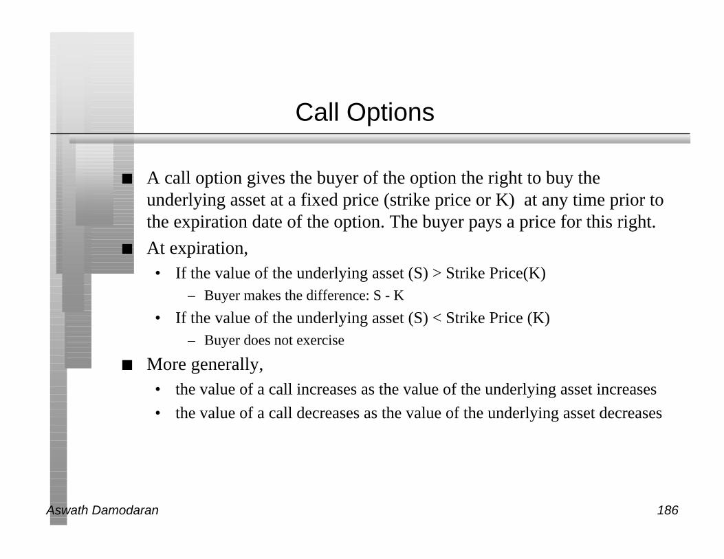
n A call option gives the buyer of the option the right to buy theunderlying asset at a fixed price (strike price or K) at any time prior tothe expiration date of the option. The buyer pays a price for this right.

n At expiration,• If the value of the underlying asset (S) > Strike Price(K)

– Buyer makes the difference: S - K

• If the value of the underlying asset (S) < Strike Price (K)– Buyer does not exercise

n More generally,• the value of a call increases as the value of the underlying asset increases

• the value of a call decreases as the value of the underlying asset decreases


Payoff Diagram on a Call

Price of underlying asset

StrikePrice

Net Payoff on Call


Put Options

n A put option gives the buyer of the option the right to sell theunderlying asset at a fixed price at any time prior to the expiration dateof the option. The buyer pays a price for this right.

n At expiration,• If the value of the underlying asset (S) < Strike Price(K)

– Buyer makes the difference: K-S

• If the value of the underlying asset (S) > Strike Price (K)– Buyer does not exercise

n More generally,• the value of a put decreases as the value of the underlying asset increases

• the value of a put increases as the value of the underlying asset decreases


Payoff Diagram on Put Option

Price of underlying asset

StrikePrice

Net PayoffOn Put


Determinants of option value

n Variables Relating to Underlying Asset• Value of Underlying Asset; as this value increases, the right to buy at a

fixed price (calls) will become more valuable and the right to sell at afixed price (puts) will become less valuable.

• Variance in that value; as the variance increases, both calls and puts willbecome more valuable because all options have limited downside anddepend upon price volatility for upside.

• Expected dividends on the asset, which are likely to reduce the priceappreciation component of the asset, reducing the value of calls andincreasing the value of puts.

n Variables Relating to Option• Strike Price of Options; the right to buy (sell) at a fixed price becomes

more (less) valuable at a lower price.

• Life of the Option; both calls and puts benefit from a longer life.

n Level of Interest Rates; as rates increase, the right to buy (sell) at afixed price in the future becomes more (less) valuable.


American versus European options: Variablesrelating to early exercise

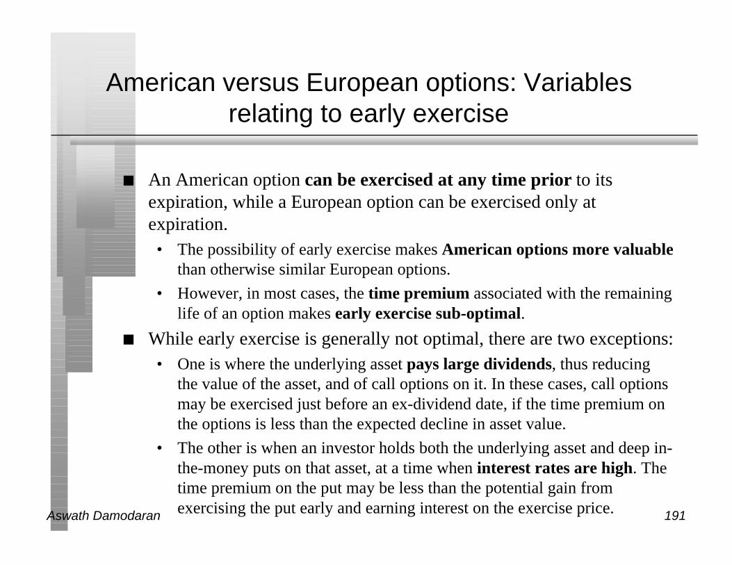
n An American option can be exercised at any time prior to itsexpiration, while a European option can be exercised only atexpiration.• The possibility of early exercise makes American options more valuable

than otherwise similar European options.

• However, in most cases, the time premium associated with the remaininglife of an option makes early exercise sub-optimal.

n While early exercise is generally not optimal, there are two exceptions:• One is where the underlying asset pays large dividends, thus reducing

the value of the asset, and of call options on it. In these cases, call optionsmay be exercised just before an ex-dividend date, if the time premium onthe options is less than the expected decline in asset value.

• The other is when an investor holds both the underlying asset and deep in-the-money puts on that asset, at a time when interest rates are high. Thetime premium on the put may be less than the potential gain fromexercising the put early and earning interest on the exercise price.


A Summary of the Determinants of OptionValue

Factor Call Value Put Value

Increase in Stock Price Increases Decreases

Increase in Strike Price Decreases Increases

Increase in variance of underlying asset Increases Increases

Increase in time to expiration Increases Increases

Increase in interest rates Increases Decreases

Increase in dividends paid Decreases Increases


Creating a replicating portfolio

n The objective in creating a replicating portfolio is to use a combinationof riskfree borrowing/lending and the underlying asset to create thesame cashflows as the option being valued.• Call = Borrowing + Buying ∆ of the Underlying Stock

• Put = Selling Short ∆ on Underlying Asset + Lending

• The number of shares bought or sold is called the option delta.

n The principles of arbitrage then apply, and the value of the option hasto be equal to the value of the replicating portfolio.


The Binomial Option Pricing Model


The Limiting Distributions….

n As the time interval is shortened, the limiting distribution, as t -> 0,can take one of two forms.• If as t -> 0, price changes become smaller, the limiting distribution is the

normal distribution and the price process is a continuous one.

• If as t->0, price changes remain large, the limiting distribution is thepoisson distribution, i.e., a distribution that allows for price jumps.

n The Black-Scholes model applies when the limiting distribution isthe normal distribution , and explicitly assumes that the price processis continuous and that there are no jumps in asset prices.


The Black-Scholes Model

n The version of the model presented by Black and Scholes wasdesigned to value European options, which were dividend-protected.

n The value of a call option in the Black-Scholes model can be writtenas a function of the following variables:S = Current value of the underlying asset

K = Strike price of the option

t = Life to expiration of the option

r = Riskless interest rate corresponding to the life of the option

σ2 = Variance in the ln(value) of the underlying asset


The Black Scholes Model

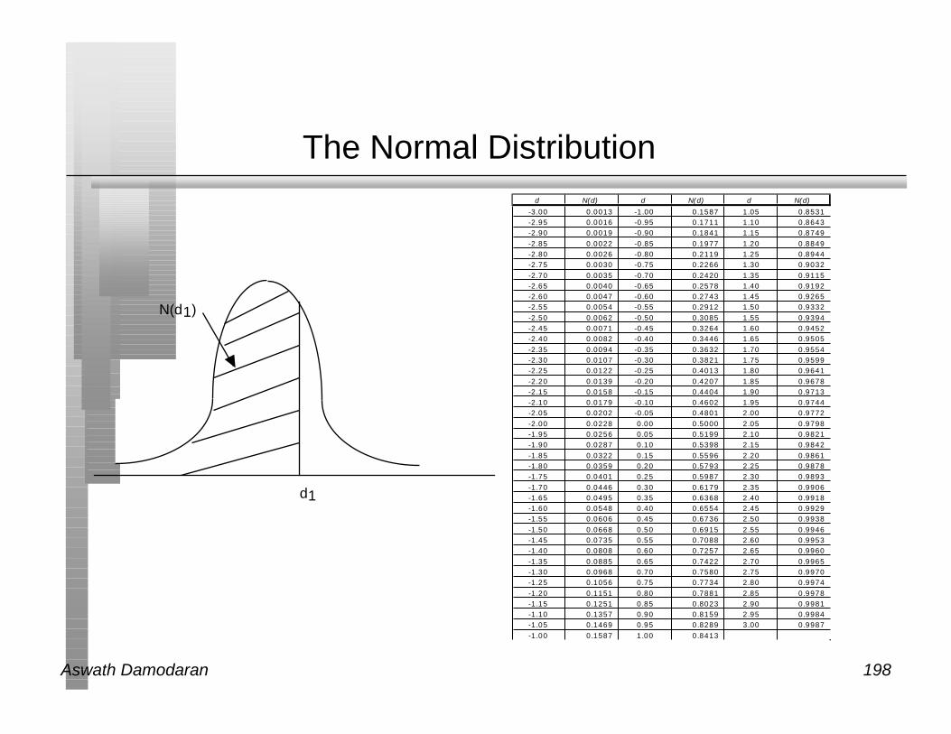
Value of call = S N (d1) - K e-rt N(d2)where,

• d2 = d1 - σ √t

n The replicating portfolio is embedded in the Black-Scholes model. Toreplicate this call, you would need to• Buy N(d1) shares of stock; N(d1) is called the option delta

• Borrow K e-rt N(d2)

d1 = ln

S

K

+ ( r +

2

2) t

t


The Normal Distributiond N(d) d N(d) d N(d)

-3.00 0.0013 -1.00 0.1587 1.05 0.8531 -2.95 0.0016 -0.95 0.1711 1.10 0.8643 -2.90 0.0019 -0.90 0.1841 1.15 0.8749 -2.85 0.0022 -0.85 0.1977 1.20 0.8849 -2.80 0.0026 -0.80 0.2119 1.25 0.8944 -2.75 0.0030 -0.75 0.2266 1.30 0.9032 -2.70 0.0035 -0.70 0.2420 1.35 0.9115 -2.65 0.0040 -0.65 0.2578 1.40 0.9192 -2.60 0.0047 -0.60 0.2743 1.45 0.9265 -2.55 0.0054 -0.55 0.2912 1.50 0.9332 -2.50 0.0062 -0.50 0.3085 1.55 0.9394 -2.45 0.0071 -0.45 0.3264 1.60 0.9452 -2.40 0.0082 -0.40 0.3446 1.65 0.9505 -2.35 0.0094 -0.35 0.3632 1.70 0.9554 -2.30 0.0107 -0.30 0.3821 1.75 0.9599 -2.25 0.0122 -0.25 0.4013 1.80 0.9641 -2.20 0.0139 -0.20 0.4207 1.85 0.9678 -2.15 0.0158 -0.15 0.4404 1.90 0.9713 -2.10 0.0179 -0.10 0.4602 1.95 0.9744 -2.05 0.0202 -0.05 0.4801 2.00 0.9772 -2.00 0.0228 0.00 0.5000 2.05 0.9798 -1.95 0.0256 0.05 0.5199 2.10 0.9821 -1.90 0.0287 0.10 0.5398 2.15 0.9842 -1.85 0.0322 0.15 0.5596 2.20 0.9861 -1.80 0.0359 0.20 0.5793 2.25 0.9878 -1.75 0.0401 0.25 0.5987 2.30 0.9893 -1.70 0.0446 0.30 0.6179 2.35 0.9906 -1.65 0.0495 0.35 0.6368 2.40 0.9918 -1.60 0.0548 0.40 0.6554 2.45 0.9929 -1.55 0.0606 0.45 0.6736 2.50 0.9938 -1.50 0.0668 0.50 0.6915 2.55 0.9946 -1.45 0.0735 0.55 0.7088 2.60 0.9953 -1.40 0.0808 0.60 0.7257 2.65 0.9960 -1.35 0.0885 0.65 0.7422 2.70 0.9965 -1.30 0.0968 0.70 0.7580 2.75 0.9970 -1.25 0.1056 0.75 0.7734 2.80 0.9974 -1.20 0.1151 0.80 0.7881 2.85 0.9978 -1.15 0.1251 0.85 0.8023 2.90 0.9981 -1.10 0.1357 0.90 0.8159 2.95 0.9984 -1.05 0.1469 0.95 0.8289 3.00 0.9987 -1.00 0.1587 1.00 0.8413

d1

N(d1)


Adjusting for Dividends

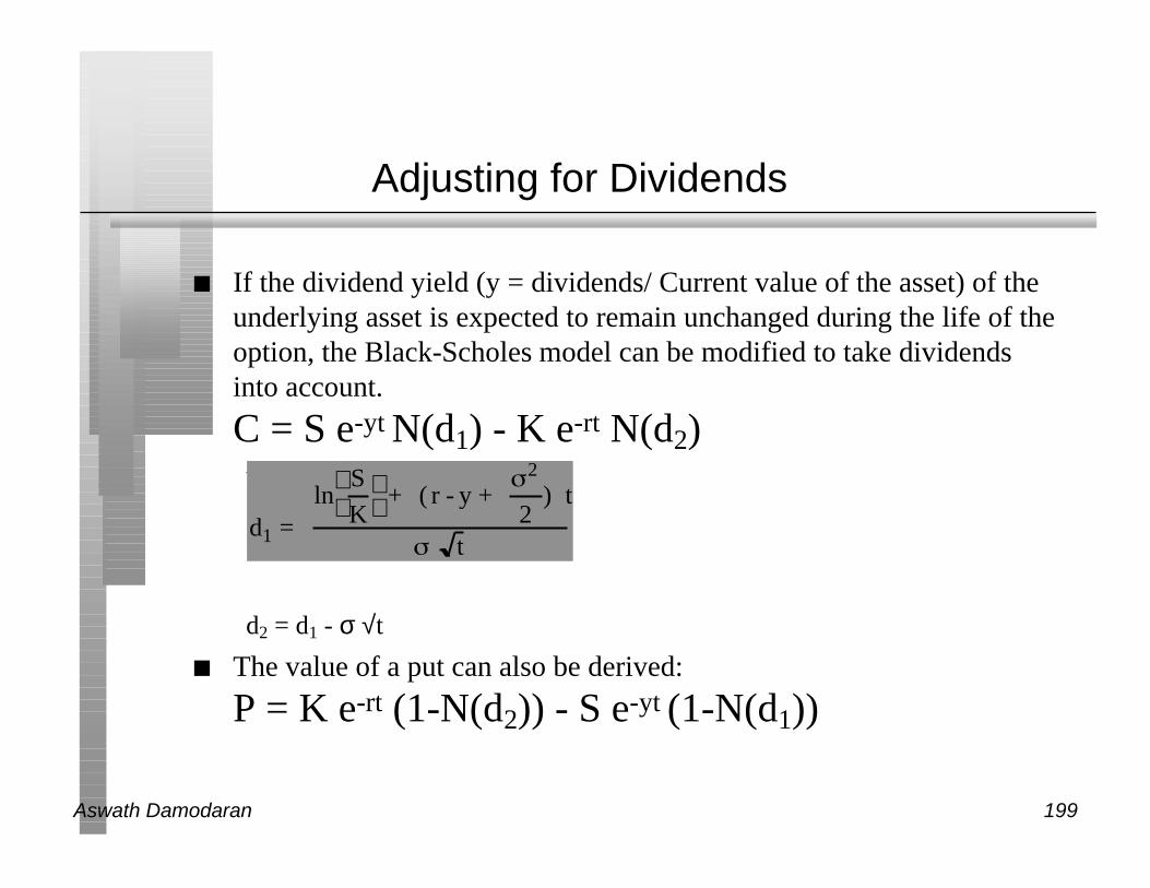
n If the dividend yield (y = dividends/ Current value of the asset) of theunderlying asset is expected to remain unchanged during the life of theoption, the Black-Scholes model can be modified to take dividendsinto account.

C = S e-yt N(d1) - K e-rt N(d2)where,

d2 = d1 - σ √t

n The value of a put can also be derived:

P = K e-rt (1-N(d2)) - S e-yt (1-N(d1))

d1 = ln

S

K

+ ( r - y +

2

2) t

t


Problems with Real Option Pricing Models

1. The underlying asset may not be traded, which makes it difficult toestimate value and variance for the underlying asset.

2. The price of the asset may not follow a continuous process, whichmakes it difficult to apply option pricing models (like the BlackScholes) that use this assumption.

3. The variance may not be known and may change over the life of theoption, which can make the option valuation more complex.

4. Exercise may not be instantaneous, which will affect the value of theoption.

5. Some real options are complex and their exercise creates other options(compound) or involve learning (learning options)


Option Pricing Applications inInvestment/Strategic Analysis


Options in Projects/Investments/Acquisitions

n One of the limitations of traditional investment analysis is that it isstatic and does not do a good job of capturing the options embedded ininvestment.• The first of these options is the option to delay taking a investment, when

a firm has exclusive rights to it, until a later date.

• The second of these options is taking one investment may allow us to takeadvantage of other opportunities (investments) in the future

• The last option that is embedded in projects is the option to abandon ainvestment, if the cash flows do not measure up.

n These options all add value to projects and may make a “bad”investment (from traditional analysis) into a good one.


The Option to Delay

n When a firm has exclusive rights to a project or product for a specificperiod, it can delay taking this project or product until a later date.

n A traditional investment analysis just answers the question of whetherthe project is a “good” one if taken today.

n Thus, the fact that a project does not pass muster today (because itsNPV is negative, or its IRR is less than its hurdle rate) does not meanthat the rights to this project are not valuable.


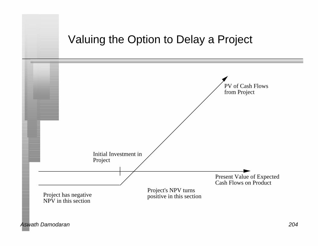
Valuing the Option to Delay a Project

Present Value of Expected Cash Flows on Product

PV of Cash Flows from Project

Initial Investment in Project

Project has negativeNPV in this section

Project's NPV turns positive in this section


Insights for Investment Analyses

n Having the exclusive rights to a product or project is valuable, even ifthe product or project is not viable today.

n The value of these rights increases with the volatility of the underlyingbusiness.

n The cost of acquiring these rights (by buying them or spending moneyon development, for instance) has to be weighed off against thesebenefits.


Example 1: Valuing product patents as options

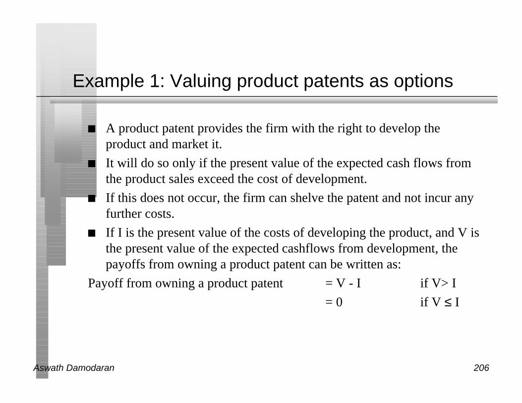
n A product patent provides the firm with the right to develop theproduct and market it.

n It will do so only if the present value of the expected cash flows fromthe product sales exceed the cost of development.

n If this does not occur, the firm can shelve the patent and not incur anyfurther costs.

n If I is the present value of the costs of developing the product, and V isthe present value of the expected cashflows from development, thepayoffs from owning a product patent can be written as:

Payoff from owning a product patent = V - I if V> I

= 0 if V ≤ I


Payoff on Product Option

Present Value ofcashflows on product

Net Payoff tointroduction

Cost of product introduction


Obtaining Inputs for Patent Valuation

Input Estimation Process

1. Value of the Underlying Asset • Present Value of Cash Inflows from taking projectnow

• This will be noisy, but that adds value.

2. Variance in value of underlying asset • Variance in cash flows of similar assets or firms• Variance in present value from capital budgeting

simulation.

3. Exercise Price on Option • Option is exercised when investment is made.• Cost of making investment on the project ; assumed

to be constant in present value dollars.

4. Expiration of the Option • Life of the patent

5. Dividend Yield • Cost of delay• Each year of delay translates into one less year of

value-creating cashflows

Annual cost of delay = 1

n


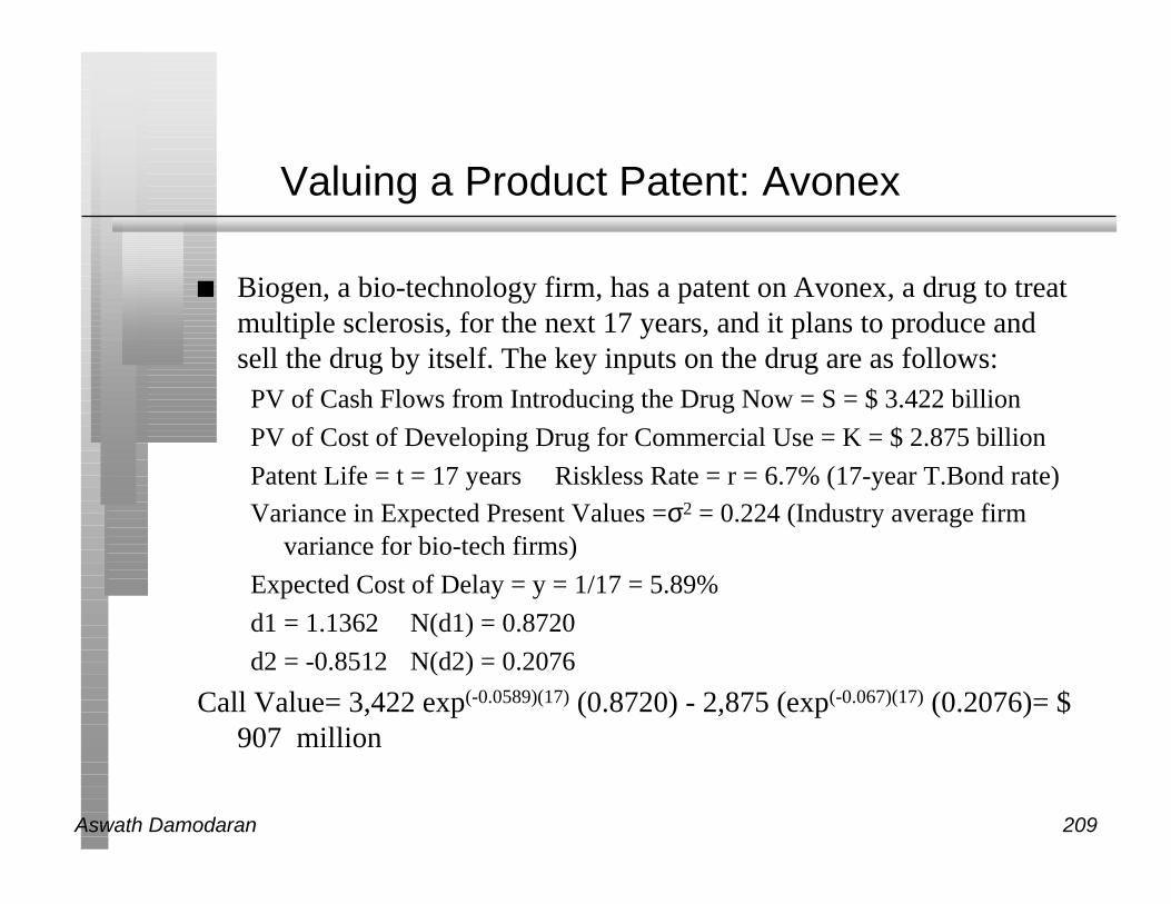
Valuing a Product Patent: Avonex

n Biogen, a bio-technology firm, has a patent on Avonex, a drug to treatmultiple sclerosis, for the next 17 years, and it plans to produce andsell the drug by itself. The key inputs on the drug are as follows:PV of Cash Flows from Introducing the Drug Now = S = $ 3.422 billion

PV of Cost of Developing Drug for Commercial Use = K = $ 2.875 billion

Patent Life = t = 17 years Riskless Rate = r = 6.7% (17-year T.Bond rate)

Variance in Expected Present Values =σ2 = 0.224 (Industry average firmvariance for bio-tech firms)

Expected Cost of Delay = y = 1/17 = 5.89%

d1 = 1.1362 N(d1) = 0.8720

d2 = -0.8512 N(d2) = 0.2076

Call Value= 3,422 exp(-0.0589)(17) (0.8720) - 2,875 (exp(-0.067)(17) (0.2076)= $907 million


Valuing a firm with patents

n The value of a firm with a substantial number of patents can bederived using the option pricing model.

Value of Firm = Value of commercial products (using DCF value

+ Value of existing patents (using option pricing)

+ (Value of New patents that will be obtained in the future – Cost of obtaining these patents)

n The last input measures the efficiency of the firm in converting itsR&D into commercial products. If we assume that a firm earns its costof capital from research, this term will become zero.

n If we use this approach, we should be careful not to double count andallow for a high growth rate in cash flows (in the DCF valuation).


Value of Biogen’s existing products

• Biogen had two commercial products (a drug to treat Hepatitis B andIntron) at the time of this valuation that it had licensed to otherpharmaceutical firms.

• The license fees on these products were expected to generate $ 50million in after-tax cash flows each year for the next 12 years. Tovalue these cash flows, which were guaranteed contractually, theriskless rate of 6.7% was used:

Present Value of License Fees = $ 50 million (1 – (1.067)-12)/.067

= $ 403.56 million


Value of Biogen’s Future R&D

• Biogen continued to fund research into new products, spending about$ 100 million on R&D in the most recent year. These R&D expenseswere expected to grow 20% a year for the next 10 years, and 5%thereafter.

• It was assumed that every dollar invested in research would create $1.25 in value in patents (valued using the option pricing modeldescribed above) for the next 10 years, and break even after that (i.e.,generate $ 1 in patent value for every $ 1 invested in R&D).

• There was a significant amount of risk associated with this componentand the cost of capital was estimated to be 15%.


Value of Future R&D

Yr Value of R&D Cost Excess Value Present Value

Patents (at 15%)

1 $ 150.00 $ 120.00 $ 30.00 $ 26.09

2 $ 180.00 $ 144.00 $ 36.00 $ 27.22

3 $ 216.00 $ 172.80 $ 43.20 $ 28.40

4 $ 259.20 $ 207.36 $ 51.84 $ 29.64

5 $ 311.04 $ 248.83 $ 62.21 $ 30.93

6 $ 373.25 $ 298.60 $ 74.65 $ 32.27

7 $ 447.90 $ 358.32 $ 89.58 $ 33.68

8 $ 537.48 $ 429.98 $ 107.50 $ 35.14

9 $ 644.97 $ 515.98 $ 128.99 $ 36.67

10 $ 773.97 $ 619.17 $ 154.79 $ 38.26

$ 318.30


Value of Biogen

n The value of Biogen as a firm is the sum of all three components – thepresent value of cash flows from existing products, the value ofAvonex (as an option) and the value created by new research:

Value = Existing products + Existing Patents + Value: Future R&D

= $ 403.56 million + $ 907 million + $ 318.30 million

= $1628.86 million

n Since Biogen had no debt outstanding, this value was divided by thenumber of shares outstanding (35.50 million) to arrive at a value pershare:

Value per share = $ 1,628.86 million / 35.5 = $ 45.88


Example 2: Valuing Natural Resource Options

n In a natural resource investment, the underlying asset is the resourceand the value of the asset is based upon two variables - the quantity ofthe resource that is available in the investment and the price of theresource.

n In most such investments, there is a cost associated with developingthe resource, and the difference between the value of the assetextracted and the cost of the development is the profit to the owner ofthe resource.

n Defining the cost of development as X, and the estimated value of theresource as V, the potential payoffs on a natural resource option can bewritten as follows:• Payoff on natural resource investment = V - X if V > X

• = 0 if V≤ X


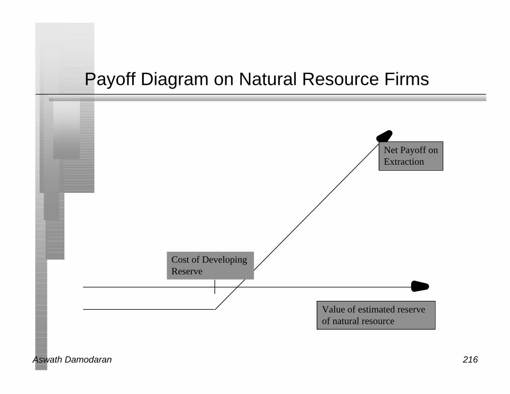
Payoff Diagram on Natural Resource Firms

Value of estimated reserveof natural resource

Net Payoff onExtraction

Cost of Developing Reserve


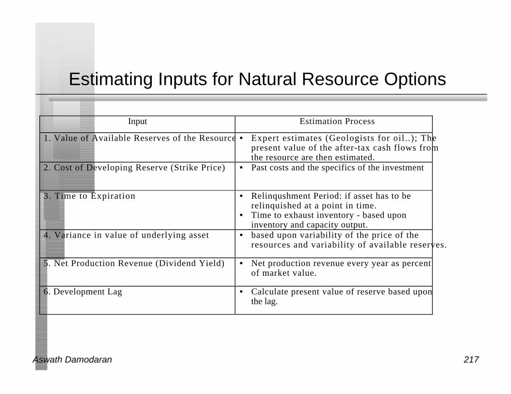
Estimating Inputs for Natural Resource Options


1. Value of Available Reserves of the Resource • Expert estimates (Geologists for oil..); Thepresent value of the after-tax cash flows fromthe resource are then estimated.

2. Cost of Developing Reserve (Strike Price) • Past costs and the specifics of the investment

3. Time to Expiration • Relinqushment Period: if asset has to berelinquished at a point in time.

• Time to exhaust inventory - based uponinventory and capacity output.

4. Variance in value of underlying asset • based upon variability of the price of theresources and variability of available reserves.

5. Net Production Revenue (Dividend Yield) • Net production revenue every year as percentof market value.

6. Development Lag • Calculate present value of reserve based uponthe lag.


Valuing an Oil Reserve

n Consider an offshore oil property with an estimated oil reserve of 50million barrels of oil, where the present value of the development costis $12 per barrel and the development lag is two years.

n The firm has the rights to exploit this reserve for the next twenty yearsand the marginal value per barrel of oil is $12 per barrel currently(Price per barrel - marginal cost per barrel).

n Once developed, the net production revenue each year will be 5% ofthe value of the reserves.

n The riskless rate is 8% and the variance in ln(oil prices) is 0.03.


Inputs to Option Pricing Model

n Current Value of the asset = S = Value of the developed reservediscounted back the length of the development lag at the dividendyield = $12 * 50 /(1.05)2 = $ 544.22

n (If development is started today, the oil will not be available for saleuntil two years from now. The estimated opportunity cost of this delayis the lost production revenue over the delay period. Hence, thediscounting of the reserve back at the dividend yield)

n Exercise Price = Present Value of development cost = $12 * 50 = $600million

n Time to expiration on the option = 20 years

n Variance in the value of the underlying asset = 0.03

n Riskless rate =8%

n Dividend Yield = Net production revenue / Value of reserve = 5%


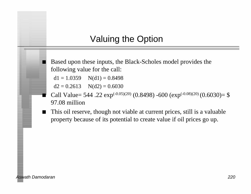
Valuing the Option

n Based upon these inputs, the Black-Scholes model provides thefollowing value for the call:d1 = 1.0359 N(d1) = 0.8498

d2 = 0.2613 N(d2) = 0.6030

n Call Value= 544 .22 exp(-0.05)(20) (0.8498) -600 (exp(-0.08)(20) (0.6030)= $97.08 million

n This oil reserve, though not viable at current prices, still is a valuableproperty because of its potential to create value if oil prices go up.


Extending the option pricing approach to valuenatural resource firms

n Since the assets owned by a natural resource firm can be viewedprimarily as options, the firm itself can be valued using optionpricing models.

n The preferred approach would be to consider each option separately,value it and cumulate the values of the options to get the firm value.

n Since this information is likely to be difficult to obtain for largenatural resource firms, such as oil companies, which own hundreds ofsuch assets, a variant is to value the entire firm as one option.

n A purist would probably disagree, arguing that valuing an option on aportfolio of assets (as in this approach) will provide a lower valuethan valuing a portfolio of options (which is what the naturalresource firm really own). Nevertheless, the value obtained from themodel still provides an interesting perspective on the determinants ofthe value of natural resource firms.


Inputs to the Model

Input to model Corresponding input for valuing firmValue of underlying asset Value of cumulated estimated reserves of the

resource owned by the firm, discounted back at thedividend yield for the development lag.

Exercise Price Estimated cumulated cost of developing estimatedreserves

Time to expiration on option Average relinquishment period across all reservesowned by firm (if known) or estimate of when reserves will be exhausted, given current production rates.

Riskless rate Riskless rate corresponding to life of the option

Variance in value of asset Variance in the price of the natural resource

Dividend yield Estimated annual net production revenue as percentage of value of the reserve.


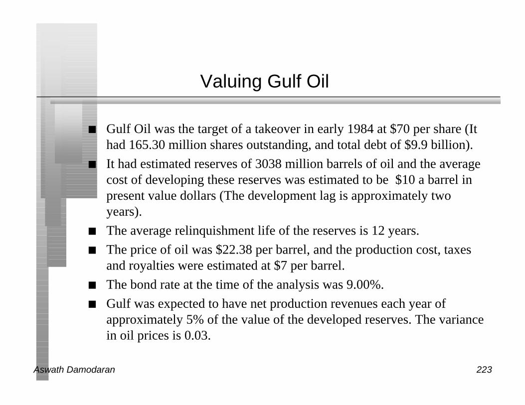
Valuing Gulf Oil

n Gulf Oil was the target of a takeover in early 1984 at $70 per share (Ithad 165.30 million shares outstanding, and total debt of $9.9 billion).

n It had estimated reserves of 3038 million barrels of oil and the averagecost of developing these reserves was estimated to be $10 a barrel inpresent value dollars (The development lag is approximately twoyears).

n The average relinquishment life of the reserves is 12 years.

n The price of oil was $22.38 per barrel, and the production cost, taxesand royalties were estimated at $7 per barrel.

n The bond rate at the time of the analysis was 9.00%.

n Gulf was expected to have net production revenues each year ofapproximately 5% of the value of the developed reserves. The variancein oil prices is 0.03.


Valuing Undeveloped Reserves

• Value of underlying asset = Value of estimated reserves discounted backfor period of development lag= 3038 * ($ 22.38 - $7) / 1.052 = $42,380.44

• Exercise price = Estimated development cost of reserves = 3038 * $10 =$30,380 million

• Time to expiration = Average length of relinquishment option = 12 years

• Variance in value of asset = Variance in oil prices = 0.03

• Riskless interest rate = 9%

• Dividend yield = Net production revenue/ Value of developed reserves =5%

n Based upon these inputs, the Black-Scholes model provides thefollowing value for the call:d1 = 1.6548 N(d1) = 0.9510

d2 = 1.0548 N(d2) = 0.8542

n Call Value= 42,380.44 exp(-0.05)(12) (0.9510) -30,380 (exp(-0.09)(12)

(0.8542)= $ 13,306 million


Valuing Gulf Oil

n In addition, Gulf Oil had free cashflows to the firm from its oil and gasproduction of $915 million from already developed reserves and thesecashflows are likely to continue for ten years (the remaining lifetime ofdeveloped reserves).

n The present value of these developed reserves, discounted at theweighted average cost of capital of 12.5%, yields:• Value of already developed reserves = 915 (1 - 1.125-10)/.125 = $5065.83

n Adding the value of the developed and undeveloped reservesValue of undeveloped reserves = $ 13,306 million

Value of production in place = $ 5,066 million

Total value of firm = $ 18,372 million

Less Outstanding Debt = $ 9,900 million

Value of Equity = $ 8,472 million

Value per share = $ 8,472/165.3 = $51.25


The Option to Expand/Take Other Projects

n Taking a project today may allow a firm to consider and take othervaluable projects in the future.

n Thus, even though a project may have a negative NPV, it may be aproject worth taking if the option it provides the firm (to take otherprojects in the future) provides a more-than-compensating value.

n These are the options that firms often call “strategic options” and useas a rationale for taking on “negative NPV” or even “negative return”projects.


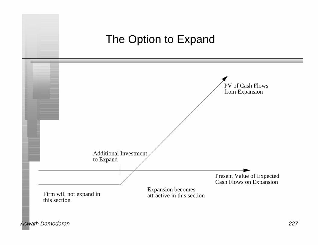
The Option to Expand

Present Value of Expected Cash Flows on Expansion

PV of Cash Flows from Expansion

Additional Investment to Expand

Firm will not expand inthis section

Expansion becomes attractive in this section


An Example of an Expansion Option

n Ambev is considering introducing a soft drink to the U.S. market. Thedrink will initially be introduced only in the metropolitan areas of theU.S. and the cost of this “limited introduction” is $ 500 million.

n A financial analysis of the cash flows from this investment suggeststhat the present value of the cash flows from this investment to Ambevwill be only $ 400 million. Thus, by itself, the new investment has anegative NPV of $ 100 million.

n If the initial introduction works out well, Ambev could go ahead witha full-scale introduction to the entire market with an additionalinvestment of $ 1 billion any time over the next 5 years. While thecurrent expectation is that the cash flows from having this investmentis only $ 750 million, there is considerable uncertainty about both thepotential for the drink, leading to significant variance in this estimate.


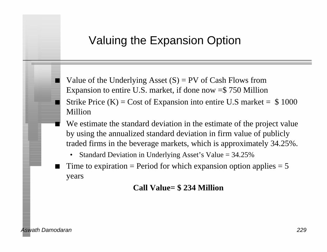
Valuing the Expansion Option

n Value of the Underlying Asset (S) = PV of Cash Flows fromExpansion to entire U.S. market, if done now =$ 750 Million

n Strike Price (K) = Cost of Expansion into entire U.S market = $ 1000Million

n We estimate the standard deviation in the estimate of the project valueby using the annualized standard deviation in firm value of publiclytraded firms in the beverage markets, which is approximately 34.25%.• Standard Deviation in Underlying Asset’s Value = 34.25%

n Time to expiration = Period for which expansion option applies = 5years

Call Value= $ 234 Million


Considering the Project with Expansion Option

n NPV of Limited Introduction = $ 400 Million - $ 500 Million = - $ 100Million

n Value of Option to Expand to full market= $ 234 Million

n NPV of Project with option to expand = - $ 100 million + $ 234 million

= $ 134 million

n Invest in the project


The Link to Strategy

n In many investments, especially acquisitions, strategic options orconsiderations are used to take investments that otherwise do not meetfinancial standards.

n These strategic options or considerations are usually related to theexpansion option described here. The key differences are as follows:• Unlike “strategic options” which are usually qualitative and not valued,

expansion options can be assigned a quantitative value and can be broughtinto the investment analysis.

• Not all “strategic considerations” have option value. For an expansionoption to have value, the first investment (acquisition) must be necessaryfor the later expansion (investment). If it is not, there is no option valuethat can be added on to the first investment.


The Exclusivity Requirement in Option Value

An Exclusive Right toSecond Investment

A Zero competitiveadvantage on Second Investment

100% of option valueNo option value

Increasing competitive advantage/ barriers to entry

Pharmaceuticalpatents

TelecomLicenses

Brand Name

TechnologicalEdge

First-Mover

Second Investment has zero excess returns

Second investmenthas large sustainableexcess return

Option has no value Option has high value

Is the first investment necessary for the second investment?

Pre-RequisitNot necessary


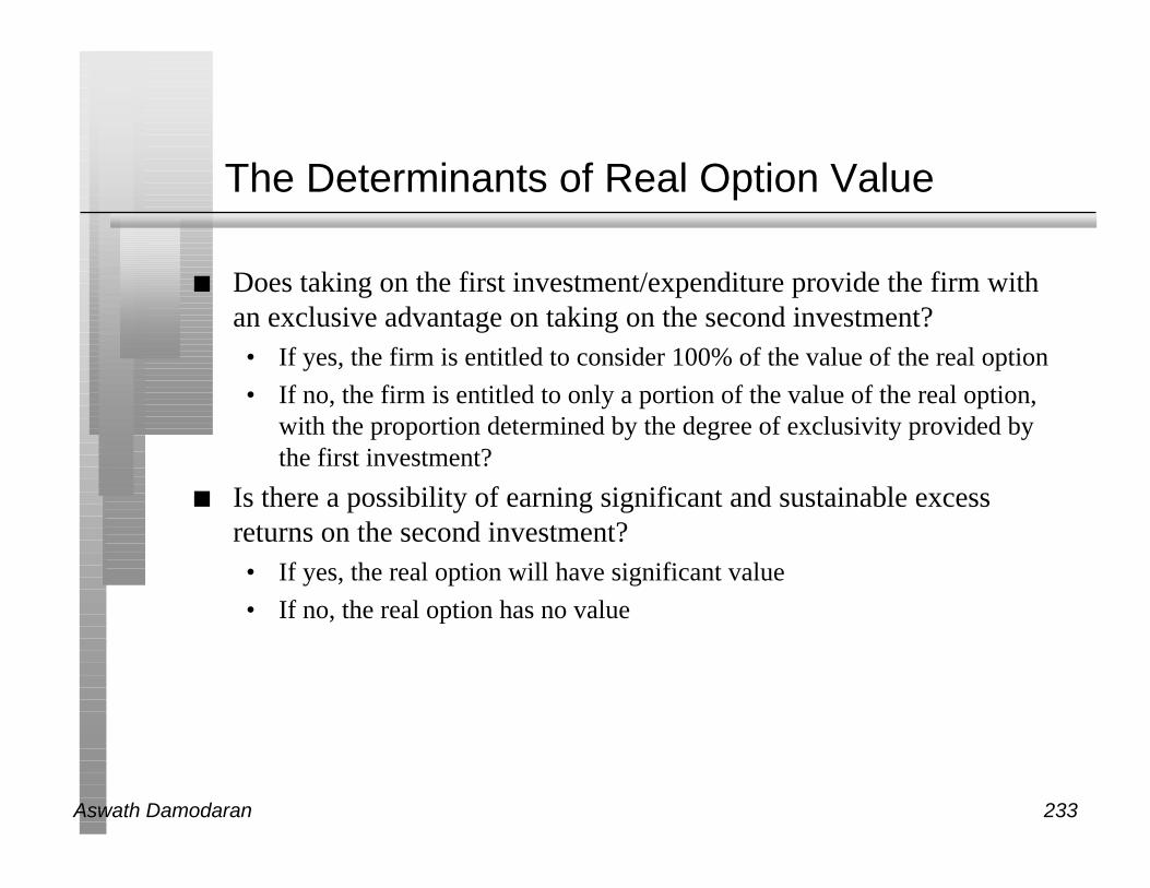
The Determinants of Real Option Value

n Does taking on the first investment/expenditure provide the firm withan exclusive advantage on taking on the second investment?• If yes, the firm is entitled to consider 100% of the value of the real option

• If no, the firm is entitled to only a portion of the value of the real option,with the proportion determined by the degree of exclusivity provided bythe first investment?

n Is there a possibility of earning significant and sustainable excessreturns on the second investment?• If yes, the real option will have significant value

• If no, the real option has no value


Internet Firms as Options

n Some analysts have justified the valuation of internet firms on thebasis that you are buying the option to expand into a very large market.What do you think of this argument?• Is there an option to expand embedded in these firms?

• Is it a valuable option?


The Option to Abandon

n A firm may sometimes have the option to abandon a project, if thecash flows do not measure up to expectations.

n If abandoning the project allows the firm to save itself from furtherlosses, this option can make a project more valuable.

Present Value of Expected Cash Flows on Project

PV of Cash Flows from Project

Cost of Abandonment


Valuing the Option to Abandon

n Airbus is considering a joint venture with Lear Aircraft to produce asmall commercial airplane (capable of carrying 40-50 passengers onshort haul flights)• Airbus will have to invest $ 500 million for a 50% share of the venture

• Its share of the present value of expected cash flows is 480 million.

n Lear Aircraft, which is eager to enter into the deal, offers to buyAirbus’s 50% share of the investment anytime over the next five yearsfor $ 400 million, if Airbus decides to get out of the venture.

n A simulation of the cash flows on this time share investment yields avariance in the present value of the cash flows from being in thepartnership is 0.16.

n The project has a life of 30 years.


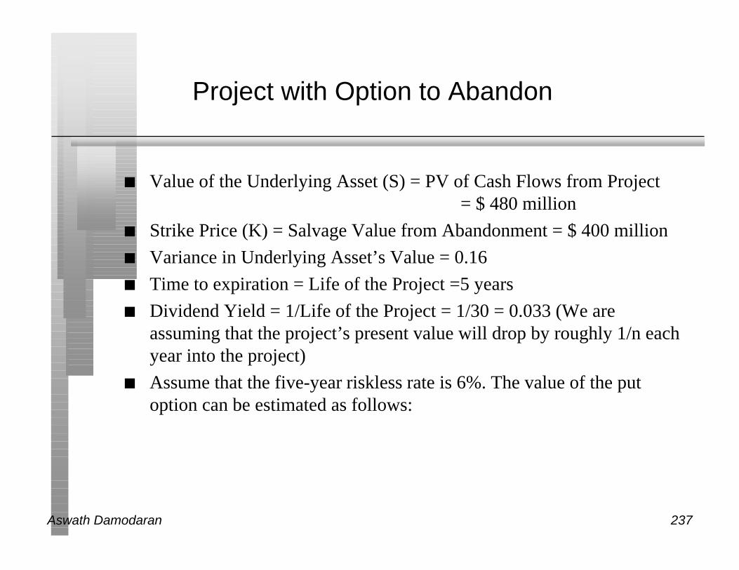
Project with Option to Abandon

n Value of the Underlying Asset (S) = PV of Cash Flows from Project= $ 480 million

n Strike Price (K) = Salvage Value from Abandonment = $ 400 million

n Variance in Underlying Asset’s Value = 0.16

n Time to expiration = Life of the Project =5 years

n Dividend Yield = 1/Life of the Project = 1/30 = 0.033 (We areassuming that the project’s present value will drop by roughly 1/n eachyear into the project)

n Assume that the five-year riskless rate is 6%. The value of the putoption can be estimated as follows:


Should Airbus enter into the joint venture?

n Value of Put =Ke-rt (1-N(d2))- Se-yt (1-N(d1))

=400 (exp(-0.06)(5) (1-0.7496) - 480 exp(-0.033)(5) (1-0.9105)

= $ 73.23 million

n The value of this abandonment option has to be added on to the netpresent value of the project of -$ 20 million, yielding a total netpresent value with the abandonment option of $ 53.23 million.


Implications for Investment Analysis

n Having a option to abandon a project can make otherwise unacceptableprojects acceptable.

n Actions that increase the value of the abandonment option include• More cost flexibility, that is, making more of the costs of the projects into

variable costs as opposed to fixed costs.

• Fewer long-term contracts/obligations with employees and customers,since these add to the cost of abandoning a project

• Finding partners in the investment, who are willing to acquire yourinvestment in the future

n These actions will undoubtedly cost the firm some value, but this hasto be weighed off against the increase in the value of the abandonmentoption.


Option Pricing Applications in the CapitalStructure Decision


Options in Capital Structure

n The most direct applications of option pricing in capital structuredecisions is in the design of securities. In fact, most complex financialinstruments can be broken down into some combination of a simplebond/common stock and a variety of options.• If these securities are to be issued to the public, and traded, the options

have to be priced.

• If these are non-traded instruments (bank loans, for instance), they stillhave to be priced into the interest rate on the instrument.

n The other application of option pricing is in valuing flexibility. Often,firms preserve debt capacity or hold back on issuing debt because theywant to maintain flexibility.


The Value of Flexibility

n Firms maintain excess debt capacity or larger cash balances than arewarranted by current needs, to meet unexpected future requirements.

n While maintaining this financing flexibility has value to firms, it alsohas a cost; the excess debt capacity implies that the firm is giving upsome value and has a higher cost of capital.

n The value of flexibility can be analyzed using the option pricingframework; a firm maintains large cash balances and excess debtcapacity in order to have the option to take projects that might arise inthe future.


Determinants of Value of Flexibility Option

n Quality of the Firm’s Projects: It is the excess return that the firmearns on its projects that provides the value to flexibility. Other thingsremaining equal, firms operating in businesses where projects earnsubstantially higher returns than their hurdle rates should valueflexibility more than those that operate in stable businesses whereexcess returns are small.

n Uncertainty about Future Projects: If flexibility is viewed as anoption, its value will increase when there is greater uncertainty aboutfuture projects; thus, firms with predictable capital expenditures andexcess returns should value flexibility less than those with highvariability in both of those variables.


Value of Flexibility as an Option

n Consider a firm that has expected reinvestment needs of X each year,with a standard deviation in that value of σX. These externalreinvestments include both internal projects and acquisitions.

n Assume that the firm can raise L from internal cash flows and itsnormal access to capital markets. (Normal access refers to the externalfinancing that is used by a firm each year)

n Excess debt capacity becomes useful if external reinvestment needsexceed the firm’s internal funds.

If X > L: Excess debt capacity can be used to cover the difference andinvest in projects

If X<L: Excess debt capacity remains unused (with an associated cost)


What happens when you make the investment?

n If the investment earns excess returns, the firm’s value will increase bythe present value of these excess returns over time. If we assume thatthe excess return each year is constant and perpetual, the present valueof the excess returns that would be earned can be written as:

Value of investment = (ROC - Cost of capital)/ Cost of capital

n The value of the investments that you can take because you haveexcess debt capacity becomes the payoff to maintaining excess debtcapacity.

If X > L: [(ROC - Cost of capital)/ Cost of capital] New investments

If X<L: 0


The Value of Flexibility

Actual ReinvestmentNeeds

Expected (Normal) Reinvestment Needs that can be financed without flexibility

Cost of Maintaining Financing Flexibility

Use financing flexibilityto take unanticipatedinvestments (acquisitions)

Payoff: (S-K)*Excess Return/WACC

Excess Return/WACC = PV of excess returns in perpetutity


Disney’s Optimal Debt Ratio

Debt Ratio Cost of Equity Cost of Debt Cost of Capital0.00% 13.00% 4.61% 13.00%10.00% 13.43% 4.61% 12.55%Current:18%13.85% 4.80% 12.22%20.00% 13.96% 4.99% 12.17%30.00% 14.65% 5.28% 11.84%40.00% 15.56% 5.76% 11.64%50.00% 16.85% 6.56% 11.70%60.00% 18.77% 7.68% 12.11%70.00% 21.97% 7.68% 11.97%80.00% 28.95% 7.97% 12.17%90.00% 52.14% 9.42% 13.69%


Inputs to Option Valuation Model

n One way to think about firms that preserve debt capacity because theywant flexibility is that they are foregoing use this debt to invest inexisting projects at existing excess returns because they think that theymight have an increase in either investment needs or excess returns.

n To value flexibility as a percent of firm value (as an annual cost), thesewould be the inputs to the model:• S = Expected Reinvestment needs as percent of Firm Value

• K = Expected Reinvestment needs that can be financed without financingflexibility

• t = 1 year

σ2 = Variance in ln(Net Capital Expenditures)

n Once this option has been valued, estimate the present value of theexcess returns that will be gained by taking the additional investmentsby multiplying by (ROC - WACC)/WACC


The Inputs for Disney

n Expected reinvestment needs as a percent of firm value:• Over the last 5 years, reinvestment (net cap ex, acquisitions and changes

in working capital) has been approximately 5.3% of firm value

• I am assuming that this is the expected reinvestment need; the variance inln(reinvestment) over the last 5 years is 0.375

n Reinvestment needs that can be financed without flexibility.• We looked at internal funds, after debt payments but before reinvestment

needs, as a percent of firm value over the last 5 years. (Internal funds =(Net Income + Depreciation)/Market Value of the Firm)

• We looked at net debt financing each period, as a percent of firm value (asa measure of access to external financing each year). (New Debt - DebtRepaid)/Market Value of Firm)

• Reinvestment needs that can be financed without flexibility = (NetIncome + Depreciation + Net Debt Issued)/Market Value of Firm

• This number has averaged 4.8%, over the last 5 years


Valuing Flexibility at Disney

The value of flexibility as a percentage of firm value can be estimated asfollows:

n S = 5.3%

n K = 4.8%

n t = 1 year

n σ2 = 0.375 ( Variance in ln(Reinvestment Needs/Firm Value))

The value of an option with these characteristics is 1.6092%

n Disney earns 18.69% on its projects has a cost of capital of 12.22%.The excess return (annually) is 6.47%.

Value of Flexibility (annual)= 1.6092%(.0647/.1222) = 0.85 % of valuen Disney’s cost of capital at its optimal debt ratio is 11.64%. The cost it

incurs to maintain flexibility is therefore 0.58% annually (12.22%-11.64%). It therefore pays to maintain flexibility.


Determinants of the Value of Flexibility

n Capacity to raise funds to meet financing needs: The greater thecapacity to raise funds, either internally or externally, the less the valueof flexibility.• 1.1: Firms with significant internal operating cash flows should value

flexibility less than firms with small or negative operating cash flows.

• 1.2: Firms with easy access to financial markets should have a lower valuefor flexibility than firms without that access.

n Unpredictability of reinvestment needs: The more unpredictable thereinvestment needs of a firm, the greater the value of flexibility.

n Capacity to earn excess returns: The greater the capacity to earn excessreturns, the greater the value of flexibility.• 1.3: Firms that do not have the capacity to earn or sustain excess returns

get no value from flexibility.


Option Pricing Applications in Valuation

Equity Value in Deeply Troubled Firms

Value of Undeveloped Reserves for Natural Resource Firm

Value of Patent/License


Option Pricing Applications in Equity Valuation

n Equity in a troubled firm (i.e. a firm with high leverage, negativeearnings and a significant chance of bankruptcy) can be viewed as acall option, which is the option to liquidate the firm.

n Natural resource companies, where the undeveloped reserves can beviewed as options on the natural resource.

n Start-up firms or high growth firms which derive the bulk of theirvalue from the rights to a product or a service (eg. a patent)


Valuing Equity as an option

n The equity in a firm is a residual claim, i.e., equity holders lay claimto all cashflows left over after other financial claim-holders (debt,preferred stock etc.) have been satisfied.

n If a firm is liquidated, the same principle applies, with equity investorsreceiving whatever is left over in the firm after all outstanding debtsand other financial claims are paid off.

n The principle of limited liability, however, protects equity investorsin publicly traded firms if the value of the firm is less than the value ofthe outstanding debt, and they cannot lose more than their investmentin the firm.


Equity as a call option

n The payoff to equity investors, on liquidation, can therefore be writtenas:

Payoff to equity on liquidation = V - D if V > D

= 0 if V ≤ D

where,

V = Value of the firm

D = Face Value of the outstanding debt and other external claims

n A call option, with a strike price of K, on an asset with a current valueof S, has the following payoffs:

Payoff on exercise = S - K if S > K

= 0 if S ≤ K


Payoff Diagram for Liquidation Option

Value of firm

Net Payoffon Equity

Face Valueof Debt


Application to valuation: A simple example

n Assume that you have a firm whose assets are currently valued at $100million and that the standard deviation in this asset value is 40%.

n Further, assume that the face value of debt is $80 million (It is zerocoupon debt with 10 years left to maturity).

n If the ten-year treasury bond rate is 10%,• how much is the equity worth?

• What should the interest rate on debt be?


Model Parameters

n Value of the underlying asset = S = Value of the firm = $ 100 million

n Exercise price = K = Face Value of outstanding debt = $ 80 million

n Life of the option = t = Life of zero-coupon debt = 10 years

n Variance in the value of the underlying asset = σ2 = Variance in firmvalue = 0.16

n Riskless rate = r = Treasury bond rate corresponding to option life =10%


Valuing Equity as a Call Option

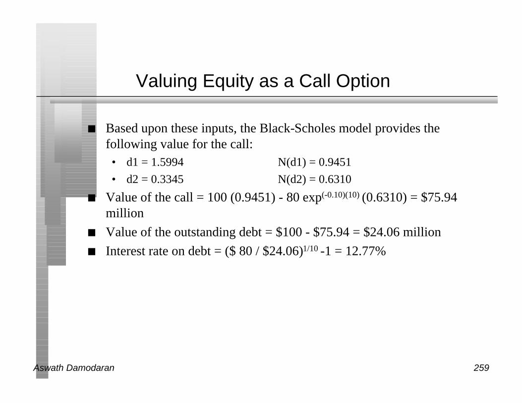
n Based upon these inputs, the Black-Scholes model provides thefollowing value for the call:• d1 = 1.5994 N(d1) = 0.9451

• d2 = 0.3345 N(d2) = 0.6310

n Value of the call = 100 (0.9451) - 80 exp(-0.10)(10) (0.6310) = $75.94million

n Value of the outstanding debt = $100 - $75.94 = $24.06 million

n Interest rate on debt = ($ 80 / $24.06)1/10 -1 = 12.77%


The Effect of Catastrophic Drops in Value

n Assume now that a catastrophe wipes out half the value of this firm(the value drops to $ 50 million), while the face value of the debtremains at $ 80 million. What will happen to the equity value of thisfirm?

o It will drop in value to $ 25.94 million [ $ 50 million - market value ofdebt from previous page]

o It will be worth nothing since debt outstanding > Firm Value

o It will be worth more than $ 25.94 million


Illustration : Value of a troubled firm

n Assume now that, in the previous example, the value of the firm werereduced to $ 50 million while keeping the face value of the debt at $80million.

n This firm could be viewed as troubled, since it owes (at least in facevalue terms) more than it owns.

n The equity in the firm will still have value, however.


Valuing Equity in the Troubled Firm

n Value of the underlying asset = S = Value of the firm = $ 50 million

n Exercise price = K = Face Value of outstanding debt = $ 80 million

n Life of the option = t = Life of zero-coupon debt = 10 years

n Variance in the value of the underlying asset = σ2 = Variance in firmvalue = 0.16

n Riskless rate = r = Treasury bond rate corresponding to option life =10%


The Value of Equity as an Option

n Based upon these inputs, the Black-Scholes model provides thefollowing value for the call:• d1 = 1.0515 N(d1) = 0.8534

• d2 = -0.2135 N(d2) = 0.4155

n Value of the call = 50 (0.8534) - 80 exp(-0.10)(10) (0.4155) = $30.44million

n Value of the bond= $50 - $30.44 = $19.56 million

n The equity in this firm drops by, because of the option characteristicsof equity.

n This might explain why stock in firms, which are in Chapter 11 andessentially bankrupt, still has value.


Equity value persists ..

Value of Equity as Firm Value Changes

0

10

20

30

40

50

60

70

80

100 90 80 70 60 50 40 30 20 10

Value of Firm ($ 80 Face Value of Debt)

Val

ue o

f Eq

uity


Valuing equity in a troubled firm

n The first implication is that equity will have value, even if the valueof the firm falls well below the face value of the outstanding debt.

n Such a firm will be viewed as troubled by investors, accountants andanalysts, but that does not mean that its equity is worthless.

n Just as deep out-of-the-money traded options command value becauseof the possibility that the value of the underlying asset may increaseabove the strike price in the remaining lifetime of the option, equitywill command value because of the time premium on the option(the time until the bonds mature and come due) and the possibility thatthe value of the assets may increase above the face value of the bondsbefore they come due.


Obtaining option pricing inputs - Some realworld problems

n The examples that have been used to illustrate the use of option pricingtheory to value equity have made some simplifying assumptions.Among them are the following:(1) There were only two claim holders in the firm - debt and equity.

(2) There is only one issue of debt outstanding and it can be retired at facevalue.

(3) The debt has a zero coupon and no special features (convertibility, putclauses etc.)

(4) The value of the firm and the variance in that value can be estimated.


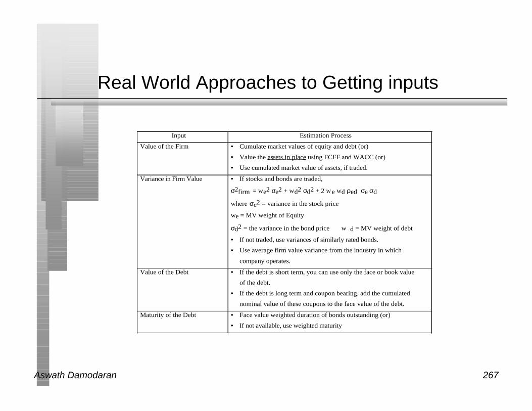
Real World Approaches to Getting inputs


Value of the Firm • Cumulate market values of equity and debt (or)

• Value the assets in place using FCFF and WACC (or)

• Use cumulated market value of assets, if traded.

Variance in Firm Value • If stocks and bonds are traded,

σ2firm = we2 σe2 + wd2 σd2 + 2 we wd ρed σe σd

where σe2 = variance in the stock price

we = MV weight of Equity

σd2 = the variance in the bond price w d = MV weight of debt

• If not traded, use variances of similarly rated bonds.

• Use average firm value variance from the industry in which

company operates.

Value of the Debt • If the debt is short term, you can use only the face or book value

of the debt.

• If the debt is long term and coupon bearing, add the cumulated

nominal value of these coupons to the face value of the debt.

Maturity of the Debt • Face value weighted duration of bonds outstanding (or)

• If not available, use weighted maturity


Valuing Equity as an option - Eurotunnel inearly 1998

n Eurotunnel has been a financial disaster since its opening• In 1997, Eurotunnel had earnings before interest and taxes of -£56 million

and net income of -£685 million

• At the end of 1997, its book value of equity was -£117 million

n It had £8,865 million in face value of debt outstanding• The weighted average duration of this debt was 10.93 years

Debt Type Face Value Duration

Short term 935 0.50

10 year 2435 6.7

20 year 3555 12.6

Longer 1940 18.2 Total £8,865 mil 10.93 years


The Basic DCF Valuation

n The value of the firm estimated using projected cashflows to the firm,discounted at the weighted average cost of capital was £2,312 million.

n This was based upon the following assumptions –• Revenues will grow 5% a year in perpetuity.

• The COGS which is currently 85% of revenues will drop to 65% ofrevenues in yr 5 and stay at that level.

• Capital spending and depreciation will grow 5% a year in perpetuity.

• There are no working capital requirements.

• The debt ratio, which is currently 95.35%, will drop to 70% after year 5.The cost of debt is 10% in high growth period and 8% after that.

• The beta for the stock will be 1.10 for the next five years, and drop to 0.8after the next 5 years.

• The long term bond rate is 6%.


Other Inputs

n The stock has been traded on the London Exchange, and theannualized std deviation based upon ln (prices) is 41%.

n There are Eurotunnel bonds, that have been traded; the annualized stddeviation in ln(price) for the bonds is 17%.• The correlation between stock price and bond price changes has been 0.5.

The proportion of debt in the capital structure during the period (1992-1996) was 85%.

• Annualized variance in firm value

= (0.15)2 (0.41)2 + (0.85)2 (0.17)2 + 2 (0.15) (0.85)(0.5)(0.41)(0.17)= 0.0335

n The 15-year bond rate is 6%. (I used a bond with a duration of roughly11 years to match the life of my option)


Valuing Eurotunnel Equity and Debt

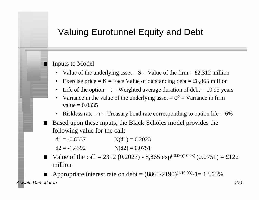
n Inputs to Model• Value of the underlying asset = S = Value of the firm = £2,312 million

• Exercise price = K = Face Value of outstanding debt = £8,865 million

• Life of the option = t = Weighted average duration of debt = 10.93 years

• Variance in the value of the underlying asset = σ2 = Variance in firmvalue = 0.0335

• Riskless rate = r = Treasury bond rate corresponding to option life = 6%

n Based upon these inputs, the Black-Scholes model provides thefollowing value for the call:d1 = -0.8337 N(d1) = 0.2023

d2 = -1.4392 N(d2) = 0.0751

n Value of the call = 2312 (0.2023) - 8,865 exp(-0.06)(10.93) (0.0751) = £122million

n Appropriate interest rate on debt = (8865/2190)(1/10.93)-1= 13.65%


Industry Name Std Dev(Equity) Std Dev(Firm) Industry Name Std Dev(Equity) Std Dev(Firm)Advertising 35.48% 27.11% Household Products 29.40% 24.91%Aerospace/Defense 37.40% 33.13% Industrial Services 43.95% 39.62%Air Transport 44.52% 33.80% Insurance (Diversified) 28.46% 26.99%Aluminum 29.20% 22.05% Insurance (Life) 30.61% 29.15%Apparel 45.25% 37.34% Insurance (Prop/Casualty) 26.98% 25.68%Auto & Truck 31.01% 23.90% Investment Co. (Domestic) 23.40% 22.28%Auto Parts (OEM) 31.21% 26.63% Investment Co. (Foreign) 28.01% 27.91%Auto Parts (Replacement) 33.28% 25.71% Investment Co. (Income) 10.95% 10.95%Bank 24.44% 22.44% Machinery 35.25% 30.94%Bank (Canadian) 21.18% 19.12% Manuf. Housing/Rec Veh 41.09% 36.00%Bank (Foreign) 23.12% 22.39% Maritime 33.85% 24.38%Bank (Midwest) 20.13% 19.15% Medical Services 63.58% 55.77%Beverage (Alcoholic) 22.21% 20.24% Medical Supplies 54.33% 50.44%Beverage (Soft Drink) 37.59% 32.50% Metal Fabricating 35.61% 32.85%Building Materials 35.68% 31.08% Metals & Mining (Div.) 55.48% 50.20%Cable TV 41.41% 21.67% Natural Gas (Distrib.) 19.35% 15.23%Canadian Energy 25.24% 21.41% Natural Gas (Diversified) 33.69% 28.21%Cement & Aggregates 32.83% 29.86% Newspaper 23.54% 19.99%Chemical (Basic) 29.43% 25.16% Office Equip & Supplies 34.40% 29.32%Chemical (Diversified) 30.87% 27.01% Oilfield Services/Equip. 43.25% 39.70%Chemical (Specialty) 33.74% 29.34% Packaging & Container 37.44% 30.32%Coal/Alternate Energy 40.48% 34.85% Paper & Forest Products 28.41% 17.50%Computer & Peripherals 64.64% 59.54% Petroleum (Integrated) 25.66% 20.98%Computer Software & Svcs 52.88% 50.35% Petroleum (Producing) 49.32% 42.47%Copper 30.41% 12.62% Precision Instrument 47.36% 44.21%Diversified Co. 42.82% 35.20% Publishing 35.89% 30.75%Drug 59.77% 58.50% R.E.I.T. 25.06% 24.52%Drugstore 47.64% 36.63% Railroad 23.73% 19.37%Electric Util. (Central) 14.93% 11.38% Recreation 50.25% 39.58%Electric Utility (East) 16.56% 11.67% Restaurant 40.12% 35.55%Electric Utility (West) 18.18% 13.80% Retail (Special Lines) 51.20% 39.98%Electrical Equipment 43.70% 39.49% Retail Building Supply 40.55% 33.95%Electronics 53.39% 48.39% Retail Store 40.14% 29.46%Entertainment 36.01% 28.95% Securities Brokerage 33.42% 22.74%Environmental 53.98% 43.74% Semiconductor 54.64% 52.72%Financial Services 36.16% 27.68% Semiconductor Cap Equip 53.41% 52.50%Food Processing 33.13% 26.83% Shoe 44.63% 40.08%Food Wholesalers 27.60% 22.11% Steel (General) 33.73% 28.96%Foreign Diversified 91.01% 44.08% Steel (Integrated) 40.34% 27.69%Foreign Electron/Entertn 34.03% 29.17% Telecom. Equipment 61.61% 56.72%Foreign Telecom. 36.18% 32.99% Telecom. Services 42.29% 35.05%Furn./Home Furnishings 34.62% 30.90% Textile 31.60% 24.12%Gold/Silver Mining 49.57% 46.46% Thrift 28.94% 26.42%Grocery 31.64% 21.84% Tire & Rubber 26.39% 23.60%Healthcare Info Systems 57.80% 54.69% Tobacco 33.85% 25.31%Home Appliance 34.82% 29.48% Toiletries/Cosmetics 42.97% 36.82%Homebuilding 43.66% 27.13% Trucking/Transp. Leasing 38.09% 29.21%Hotel/Gaming 45.01% 29.76% Utility (Foreign) 23.17% 18.34%

Water Utility 18.53% 14.16%

Documents

Option Pricing Theory and Applications - NYUadamodar/pdfiles/country/option.pdf · option, which can make the option valuation more complex. 4. Exercise may not be instantaneous ,