Embed Size (px)
Citation preview

OptionsUniversityTM Option Theory & The Greeks 1
The Option Pricing Model The basis of trading any security centers on the idea of value, and options are no different. The determination of value tells us whether or not we are getting a good deal; whether or not we are buying something low or selling it high. The determination of the value of an option is based upon a complex algorithm known as The Options Pricing Model. The Option Pricing Model calculates the values of different options. The Option Pricing Model, and there are many of them – involve complex, convoluted, and abstract math. They are not easy calculations! When we talk about the pricing model we are talking some very, very sophisticated algorithms that are probably beyond the scope of the mathematic abilities of most traders. Fear not, however, for the ability to understand the math is not the important concept here. Understanding how the model does what it does, and why it does what it does, is the important concept. Fortunately, a doctorate in mathematics is not required, but it is a little bit advanced for some people. If you are able to understand the actual math of the models, great! However, most of us are not mathematicians. Luckily, we do not need to be mathematicians. We do not need to understand how the model functions. All we need to know is what goes into each model, what comes out of it, and where certain models display weakness. It is important to know not only what the model offers in terms of price determination but also what it discerns in terms of calculating an option’s sensitivity to changing variables. If you are able to understand the math of the model, it will probably give you an advantage in understanding the pricing mechanism. However, we can know enough and understand enough about the pricing models to give us a very strong foundation in terms of what an option is, how it’s priced, how it’s going to react and its overall nature without being an expert in math. The importance here is in the way the model calculates value. The method itself offers you a glimpse of the option’s nature. Once you understand the nature of the option, then it will be that much easier to understand how the option will function, how it will react, where it will be at risk, and where it will be profitable. In order to begin our exploration into the nature of options, there are a few things we need to know about the model first.

OptionsUniversityTM Option Theory & The Greeks 2
First, you need to know that the term ‘Option Pricing Model’ refers to one of several different pricing models, each with its own mathematical algorithms. Again, we don’t need to get into the high-end mathematics but we do need to know how the models differ from each other. That could lead to a difference in pricing in certain situations. Recognizing these differences can lead to identifying a weakness, flaw or disadvantage in a certain model. Understanding that weakness or flaw means knowing which model may be more accurate at certain times and in certain ways. You need to know which model was used to determine the value of an option and recognize its advantages and disadvantages for your needs: accurate valuation. That’s how we're going to look at the pricing models. This will be broken down into 4 simple sections:
1. The fundamentals of all pricing models- what they share and the basics
upon which they were established.
2. The types of pricing models - the evolution of the various models as an answer to a flaw or lack in an earlier model.
3. Inputs into the models- what variables must be addressed to arrive at a value determination.
4. The outputs (Greeks)- what the output numbers and probabilities mean to our investment strategy.

OptionsUniversityTM Option Theory & The Greeks 3
Fundamentals of The Option Pricing Model You can best understand anything by studying its nature. The foundation of the price of options is generated from the pricing models. So, to some extent we need to understand the fundamentals of the pricing models in order to understand the nature of options. Remember that we have already stated that you do not need to understand the actual math of the model in order to understand the model, what it can do for you, and how it works. Therefore, what we are going to talk about are some of the pricing model concepts. We will discuss concepts that are inherent to all of the models. Bear in mind, all the models are connected. They are related somehow. How? Because they start at the same place – setting up a probability model to predict an expected value of an option. And they all end up at a theoretical value, which is a value that an option should be worth. So they are starting from the same place (probability), and trying to get to the same place (value determination). Let’s begin our talk about the fundamentals of the Option Pricing Models. Fundamentals of The Options Pricing Models One thing that links all these models together is the fact that, in essence, they are all probability models. Probability is a measure of the likelihood of something happening. The pricing models all try to determine what the percentage chance of an outcome will be. They are trying to calculate the percentage chance of an option finishing in the money based upon a group of variables that you select and input into the model. We will talk a little later about the inputs of the model, but there are certain things that you have to put in for the model to generate a give-back number, which is going to be the theoretical value of the option. Another basic concept is that all these models look for an expected return, and they try to calculate the value of the option based upon that expected return. When looking at these pricing models, you have to remember that they are all linked together because they are all basically probability models. And they are all taking a look at a potential expected return of a specific option.
OptionsUniversityTM Option Theory & The Greeks 4
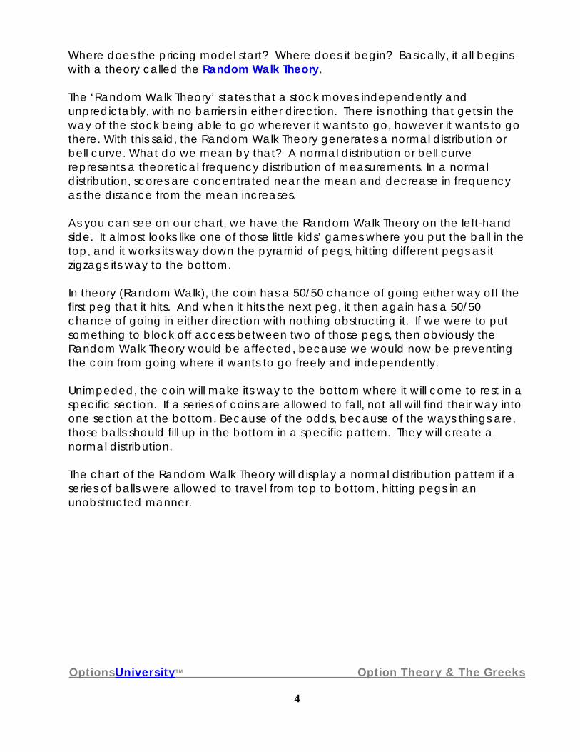
Where does the pricing model start? Where does it begin? Basically, it all begins with a theory called the Random Walk Theory. The ‘Random Walk Theory’ states that a stock moves independently and unpredictably, with no barriers in either direction. There is nothing that gets in the way of the stock being able to go wherever it wants to go, however it wants to go there. With this said, the Random Walk Theory generates a normal distribution or bell curve. What do we mean by that? A normal distribution or bell curve represents a theoretical frequency distribution of measurements. In a normal distribution, scores are concentrated near the mean and decrease in frequency as the distance from the mean increases.
As you can see on our chart, we have the Random Walk Theory on the left-hand side. It almost looks like one of those little kids’ games where you put the ball in the top, and it works its way down the pyramid of pegs, hitting different pegs as it zigzags its way to the bottom. In theory (Random Walk), the coin has a 50/50 chance of going either way off the first peg that it hits. And when it hits the next peg, it then again has a 50/50 chance of going in either direction with nothing obstructing it. If we were to put something to block off access between two of those pegs, then obviously the Random Walk Theory would be affected, because we would now be preventing the coin from going where it wants to go freely and independently. Unimpeded, the coin will make its way to the bottom where it will come to rest in a specific section. If a series of coins are allowed to fall, not all will find their way into one section at the bottom. Because of the odds, because of the ways things are, those balls should fill up in the bottom in a specific pattern. They will create a normal distribution. The chart of the Random Walk Theory will display a normal distribution pattern if a series of balls were allowed to travel from top to bottom, hitting pegs in an unobstructed manner.

OptionsUniversityTM Option Theory & The Greeks 5
This pattern is referred to as normal distribution - normal outcomes. Some of us recognize the pattern as the “bell curve.” The formal definition of a normal distribution is complicated, however, for our purposes, it is simply a measure of dispersion around the mean, or the average. That is a very simple definition of normal distribution but adequate for our use. Our market system functions under the Random Walk Theory. It is supposedly designed to allow stocks to move and flow independently and freely in any direction at any given time. Stocks will zigzag their way to a potential outcome. That is what the Random Walk Theory says. From Random Walk, we are led to the bell curve. The bell curve is a normal distribution. What the bell curve says is that among a certain amount of samples, this is the normal outcome. Normal distribution points out the normal outcome among a variety of possible outcomes. For our purposes in option pricing, the bell curve answers the question of what is the normal

OptionsUniversityTM Option Theory & The Greeks 6
outcome (or percentage chance) of the stock finishing at this price? Or what about this price? Or what about that price? The pricing model takes a look at all the different places where the stock can finish and adds the chances of the stock finishing there as described by the bell curve. It then creates theoretical option values or prices based upon the percentage chance of the option finishing in-the-money (with value) by expiration. Obviously, the bell curve or normal distribution, and its probabilities are critical to option pricing. So, let’s take a little closer look at normal distributions. Look at the charts below. What you see in front of you are two separate but similar normal distributions. Now, the term normal distribution (bell curve) does not really signify the perfect shape of the bell. What it is telling you is that it is a family of different distributions that are evenly dispersed around the mean. Evenly dispersed means that bell curves must be symmetrical. That is important because if the curves are not symmetrical, then they are not a normal distribution. And this is going to be important later because the majority of the pricing models are based upon normal distributions. If stock returns are normally distributed, then these models will work perfectly. However, if stock returns aren’t normally distributed (log-normally distributed), then these models are not going to be extremely accurate. They might be relatively accurate. They might even be very accurate, but they will not be perfectly accurate. And in certain instances, that can hurt you. Later, we are going to talk about what those instances are, and how we can properly adjust for them. But for right now, a normal distribution is any family of distributions that are symmetrical.
OptionsUniversityTM Option Theory & The Greeks 7
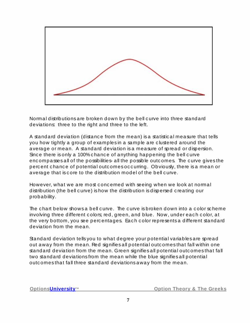
Normal distributions are broken down by the bell curve into three standard deviations: three to the right and three to the left. A standard deviation (distance from the mean) is a statistical measure that tells you how tightly a group of examples in a sample are clustered around the average or mean. A standard deviation is a measure of spread or dispersion. Since there is only a 100% chance of anything happening the bell curve encompasses all of the possibilities- all the possible outcomes. The curve gives the percent chance of potential outcomes occurring. Obviously, there is a mean or average that is core to the distribution model of the bell curve. However, what we are most concerned with seeing when we look at normal distribution (the bell curve) is how the distribution is dispersed creating our probability. The chart below shows a bell curve. The curve is broken down into a color scheme involving three different colors; red, green, and blue. Now, under each color, at the very bottom, you see percentages. Each color represents a different standard deviation from the mean. Standard deviation tells you to what degree your potential variables are spread out away from the mean. Red signifies all potential outcomes that fall within one standard deviation from the mean. Green signifies all potential outcomes that fall two standard deviations from the mean while the blue signifies all potential outcomes that fall three standard deviations away from the mean.

OptionsUniversityTM Option Theory & The Greeks 8
When we look at the bell curve above, we know that everything that is one standard deviation plus or minus from the mean (red) occurs 68.4% of the time. According to all the tests the amount of times that the potential outcome falls in between those two black lines is 68.4% of the time. That is one standard deviation from the mean. That gives you a general idea of how often the potential outcome is going to fall between those two points.
As stated, the area in green shows a two standard deviation movement from the mean. The chance of a two standard deviation move occurring is 13.5% to the downside, and 13.5% to the upside, which together, is a 27% chance. So, you have a 68.4% chance of potential outcomes landing plus or minus one standard deviation off the average. And from there you have a 27% chance of potential outcomes landing two standard deviations, plus or minus, away from the mean. Finally, you have the blue area, which is a three standard deviation movement from the mean. That will occur 4.4% of the time. In a normal distribution that is symmetrical, that 4.4% is evenly distributed - 2.2% to the left or downside, and 2.2% to the right or upside

OptionsUniversityTM Option Theory & The Greeks 9
Look at the chart above. Remember the normal distribution or bell curve and recall that standard deviation is a measure of dispersion telling you how far from the mean a certain potential outcome may lie, and the percentage chance of that event happening. You’ll see why that is important later. In options, standard deviations are known by special terms. Look at the first standard deviation - that area of 68.4% (roughly two out of three) to the right and left of the mean colored in red. That area, from an option standpoint is known as “the meat.” That is right around the at-the-money option- the area where you have the best chance of a stock price finishing. It’s the meat. The second standard deviation (shown in green) occurs 27% of the time, (13.5% upside, 13.5% downside) or approximately once in twenty events. Since there is no option term describing this specific area, it is lumped in with the “meat.” This area constitutes the slightly out of the money options.

OptionsUniversityTM Option Theory & The Greeks
10
On the two far ends, at three standard deviations (colored in blue) in either direction, (2.2% upside, 2.2% downside) are what’s commonly referred to in option talk as the “tails,” “wings” or the “outliers.” Any of these monikers may be used depending on who you talk to but, do understand, all these titles refer to the same thing. These “outliers” represent dramatic gap movements. Look back to the previous chart showing Random Walk and Normal Distribution. When you look at the normal distribution, do you see that little ball all the way on the left-hand side by itself? That represents the day that the stock has a dramatic movement, most likely a news-related gap opening. Remember, on most days, stocks only fluctuate a little bit. That is where the “meat” is. It occurs in the red area and happens 68.4% of the time. All those little balls in the area labeled 1 SD represent a day when the stock really doesn’t move much. Balls (potential outcomes) that fall within that area land in the first standard deviation that, as said, occurs 68.4% of the time. Now, the day that something dramatically bad/good happens, that little ball way over to the far side by its lonesome, that one above 2.2%, that’s that day when something really good/bad happens. So, whenever we talk about the outliers or tails, or wings, we are talking about the potential outcomes located way out to the sides. They are located in that little area labeled three standard deviations, 2.2% on either side. When you hear traders talk about tails, or my wings, or the outliers, that’s what they are talking about.

OptionsUniversityTM Option Theory & The Greeks
11
Wings are usually those days of normally news driven, dramatic gap movements, either up or down. Typically, these types of movements do not occur intraday. They happen at the stock opening the next morning either up gigantically on very, very positive news, or down gigantically on very, very negative news. So whenever you hear tails, outliers, or wings – and we will be using those terms in the future – you know what we are talking about. We are talking about the way-out-of-the-money strikes - both calls and puts. When viewing the bell curve in terms of options, the outer regions way off to the right are your way-out-of-the-money calls. The outer regions way off to the left are your way-out-of-the-money puts.

OptionsUniversityTM Option Theory & The Greeks
12
Remember, when comparing the different pricing models to each other, all pricing models are related in that they all: * Are probability models
* Seek to determine a theoretical value which says what an option should be worth
* Are based on normal distribution (bell curve dispersion around the mean)
* Require inputs of variables. Many of the option pricing models are formulated based upon an error in a previous model, a weakness in a previous model, or due to unexpected market evolution. As a result of the way that the pricing of the trading markets has evolved, the models have had to evolve and change and adapt to the different ways things are priced, the different ways things happen, and the different variables that affect the prices of options at different times. So, we’ll talk about the pricing models by giving a brief overview of several selected models, and discussing their strengths and weaknesses. This will make it possible for you to see an evolution in these models as they try to compensate for the ever changing market environment. What is important is to remember the names of the most prominent models and their unique advantages and disadvantages. Now, the first model that we want to talk about is the granddaddy of them all. It is probably the most well-known and popular model out there. It’s called the Black-Scholes Model and was formulated in 1973 by two people by the name of Fisher Black and Myron Scholes. This model won the Nobel Prize in Economics in 1997. While an award winner, the Black-Scholes had its flaws. The problem with the Black-Scholes model was that it was originally suppose to calculate the price of European-style options. European options do not allow for early exercise as do the American-style options. In this way, European-style options are very much like futures. The main problem with the Black-Scholes model is it does not account for (price) the ability of American options’ early exercise. It does not account for exercising early to collect interest rate. It also does not account for exercising early to collect the dividend. And further, as you go out over time, the model loses its integrity.

OptionsUniversityTM Option Theory & The Greeks
13
However, the Black-Scholes model has been the basis for subsequent models and remains a “granddaddy” to some of today’s more sophisticated models. Since then, the Black-Scholes model has been modified to adjust for this deficiency (Modified Black-Scholes model). Another model that was in existence during that early time was the Monte Carlo Simulation method. Credit for inventing the Monte Carlo Simulation method often goes to Stanislaw Ulam, a Polish born mathematician who worked for John von Neumann on the United States’ Manhattan Project during World War II. Ulam is primarily known for designing the hydrogen bomb with Edward Teller in 1951. He invented the Monte Carlo method in 1946 while pondering the probabilities of winning a card game of solitaire. The Monte Carlo method was extremely accurate but the problem was it was incredibly slow. Back when models were first being auditioned for their use in option pricing, computers were simply not powerful enough to warrant the use of the Monte Carlo Simulation. There were many calculations, and it was not possible to get the all those calculations done fast enough to suit the needs of traders that needed instant answers. Delays caused by the extended waiting periods cost traders money and that was unacceptable. When you observe the prices of options from the different pricing models you’ll notice that all the models value the 1st, 2nd, and 3rd month options closely. The need or the necessity to have a penny more accuracy versus waiting twenty or thirty more seconds to have your results, wasn’t worth it especially when the results were generally identical to the other models. So the Monte Carlo Simulation method, while extraordinarily accurate, was just too complex and just too slow. After the Black-Scholes model came out, and its weaknesses were identified, Cox, Ross & Rubenstein came out with the Binomial model. The Binomial model was based upon the same precepts that the Black-Scholes model was based upon. Obviously, the intent here was to develop a model that was very similar to the Black-Scholes in its speed and accuracy, but adjusted for early exercise, and for better integrity out over time. And that’s what the Binomial model does. To this day, there are probably more people using the Cox, Ross & Rubenstein Binomial model than there are using the Black-Scholes model.

OptionsUniversityTM Option Theory & The Greeks
14
The Binomial model is what is called a lattice model. It breaks down time until expiration into a series of intervals or steps. Then a tree of stock prices is produced, working forward from the present to expiration. At each step, it’s assumed that the stock price will move either up or down.
The model made the assumption that a stock will move either up or down, from one level up to the next or down to the next, continuing the pattern until you can see it form a two-branch type tree or binomial tree. That was the idea of the Binomial model. Where the model did account for early exercise and where it did have better integrity out over time it was missing something. It was missing the fact that most of the time stocks don’t move! It assumed that at every level a stock either moves up or moves down to the next level. It only recognized two choices. It did not fully account for a stocks major tendency of staying still or stagnant. Not properly pricing this “lack of movement” is an obvious flaw, because studies show that most stocks only do their major movement during a couple months out of the year. Most stocks are dormant the majority of the months of the year. The response to that omission in the Binomial model was the creation of The Trinomial Model. What do you think the Trinomial model did? Instead of having two choices, and a two-branch tree, the Trinomial had three choices and a three-

OptionsUniversityTM Option Theory & The Greeks
15
branch tree. From each step, the next step could either be up a level, down a level, or straight across sideways at the same level, which happens much more often than not. So, the Trinomial model was able to account for a stock not moving. How does this difference between the Binomial and the Trinomial affect us?
A little later we’re going to talk about volatility. In the course of our discussion of volatility, we’re going to talk about something called a volatility smile. The Binomial model, as stated, does not account for the volatility smile that exists in almost all options. However, the Trinomial model does. How? The Trinomial model accepts the fact that a stock can stay still; stock does not have to move either up or down- it can move sideways! The Binomial model, by its nature, does not take that into consideration. Where the Binomial model improved on the Black-Scholes model by properly pricing the value of early expiration, it failed to see the volatility smile. The Trinomial model takes into consideration that next step, that ability for the stock not to move thus accounting for the volatility smile.

OptionsUniversityTM Option Theory & The Greeks
16
One of my favorite models is an extension of the Trinomial model. It is called the Adaptive Mesh model. The Adaptive Mesh model takes those three branches of the Trinomial and adds some twigs on them. It adds more avenues or time intervals for the stock to move than the Trinomial model. So it’s an extension. What does that extension do? Basically the Adaptive Mesh model is as quick as the Trinomial and Binomial models, and takes in account everything those models do, including the volatility smile. However, because it has more nodes – remember the Trinomial count has three, Binomial has two- the Adaptive Mesh becomes much more accurate and stays more accurate out over time, while the others lose some of their integrity. Of course, each model loses a different amount of integrity at different rates. The Adaptive Mesh however, combined all the best things of all the previous models, including the ability to price the volatility smile as the Trinomial did, but it is more accurate, and the integrity of the model stays together much further out in time. Now as I said before, these models were made a while ago. And as the markets evolve, these models have had to evolve and adapt to different situations. One thing about some of the earlier models is that they based their pricing on the fact that they felt stock returns were going to fit into a normal distribution – that bell curve we talked about. However, as time went by, studies showed that stock returns did not follow a normal distribution. So if those models are based on normal distributions, and we find that stock returns are not normally distributed (log normal), there is a flaw. The flaw had to do with a factor that had been omitted in the pricing model’s calculations. That factor was the conditions that affected distribution of the stock returns.
OptionsUniversityTM Option Theory & The Greeks
17
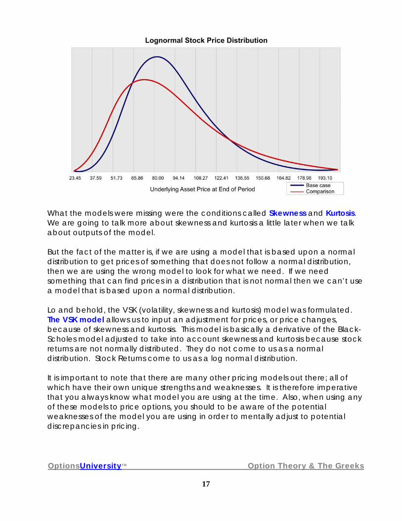
What the models were missing were the conditions called Skewness and Kurtosis. We are going to talk more about skewness and kurtosis a little later when we talk about outputs of the model. But the fact of the matter is, if we are using a model that is based upon a normal distribution to get prices of something that does not follow a normal distribution, then we are using the wrong model to look for what we need. If we need something that can find prices in a distribution that is not normal then we can’t use a model that is based upon a normal distribution. Lo and behold, the VSK (volatility, skewness and kurtosis) model was formulated. The VSK model allows us to input an adjustment for prices, or price changes, because of skewness and kurtosis. This model is basically a derivative of the Black-Scholes model adjusted to take into account skewness and kurtosis because stock returns are not normally distributed. They do not come to us as a normal distribution. Stock Returns come to us as a log normal distribution. It is important to note that there are many other pricing models out there; all of which have their own unique strengths and weaknesses. It is therefore imperative that you always know what model you are using at the time. Also, when using any of these models to price options, you should to be aware of the potential weaknesses of the model you are using in order to mentally adjust to potential discrepancies in pricing.

OptionsUniversityTM Option Theory & The Greeks
18
Inputs To The Options Pricing Model
All pricing models need inputs. In order for any of the pricing models to spit back to us the theoretical value of an option, the model needs some things put into it. It needs to base that output value upon a bunch of variables that you need to input. Let’s talk about the inputs of the option-pricing model. One of the major inputs is the stock price. Before we can determine the value of a certain option, whether a call, or a put, we need to know where the stock is because we know the stock price is going to affect that option price. We have to input a stock price. Now, when we speak of inputting the stock price (which happens to be one of the heaviest weighted factors in option price determination) we are talking about the current stock price. It is important to note that this does not specifically mean the last sale. A trader/investor may use their knowledge of the market to lean to a price toward the bid (if the stock looks heavy) or the offer (if the stock looks light) in order to predict the stocks next move or expected direction. Proper anticipation could get you a little better price in the option. As important as stock price is to an option’s price, Volatility is just as important. There are several different types or definitions of volatility. For the purposes of pricing model inputs, we will want to concentrate on forecast volatility. Forecast volatility is our personal volatility estimate. That is what we feel will be the volatility level for a specific period of time in the future. That specific time should coincide with the length of time to expiration of the particular option we are looking at. Obviously, using a volatility estimate for the next two months will not be adequate in pricing a nine-month option. For proper or reasonable accuracy, we would need to consider what we feel the volatility level will be for the whole nine-month period, not just two. There are several models designed to help you properly estimate what future volatility is most likely going to be. The use of these volatility estimators can be quite helpful. Now, regardless of how we choose to estimate or calculate our forecast volatility, we need to come up with a specific volatility level that we will plug into the model in order to allow the model to do its calculations and spit out to us the all important theoretical value. Therefore, the accuracy of this approximated volatility speculation is critical to the legitimacy of the pricing. This, in turn, will directly affect the profit potential of the trade.

OptionsUniversityTM Option Theory & The Greeks
19
Another important input is the Strike Price. Which strike are we talking about? Are we talking about an option with a strike price of 20, of 30, or of 70? We have to input the strike price that we are talking about. Obviously, different strike prices refer to different options and thus to different option values. Another input component of the model is carry cost -- Interest Rate and Dividend. You might wonder why. The importance of interest rate and dividend is that they are components of what is called ‘Cost Of Carry.’ You might wonder why it is important to include them? The reason it is important to include them is that an option’s price is going to be based on the stock’s price as stated above. Anything that can directly affect the stock’s price outside of supply and demand will affect the option’s price indirectly through the stock price and has to be accounted for in the model. You might ask how interest rate affects the stock price. Well, if you are going to carry a long stock position or if you’re going to buy a stock you are either going to put out interest rate or no longer receive interest rate. Think about it. You have money in your account. While that cash is in the account what does it collect? It collects interest! Now, we take that cash out of the account and we buy stock with it. We had $20,000 collecting interest; we now move that $20,000 over and put it into stock. It is still $20,000, but it is $20,000 worth of stock, not cash. Stock does not earn interest, cash does. Now, that $20,000 is no longer earning interest. When you use that cash to buy that stock, you are no longer gaining interest at a specific rate. That indirectly affects the return you can expect from your stock purchase. You are already losing the interest you could have earned. The stock will have to outperform that interest rate just to break even. So, in essence, lost interest is a cost of stock ownership. In theory, if it affects the price of the stock purchase, it will indirectly affect the price of the option. What if the stock was purchased on margin instead of with cash? If the stock was bought on margin, then money was borrowed to purchase the stock. That is what a margin account does. If money is borrowed to buy the stock, interest must be paid on the money borrowed. What about selling a stock? If you own a stock, you are not getting interest on the money tied up in the stock. However, if that stock is sold and the money is put into an account, then that cash starts to gain interest. What if you sold a stock short on margin?
OptionsUniversityTM Option Theory & The Greeks
20
When you sell the stock, you receive money into your account for that sale, and that money will gain some interest because it’s sitting in an account as cash. So, interest rate is an important input into the pricing model. Dividends are the other piece of our two-headed ‘cost of carry’ monster. Carry cost consists of interest and dividend. Why is dividend an input of the model? Dividend, in fact, directly affects the price of the stock. The value of any stock is basically the value of the all the company’s assets minus liabilities. If that company were to take money out of its cash account and hand it to all of its share holders, like it does in a dividend, that stock will now be worth less by the amount of the dividend paid. Cash is an asset so if the company pays out a dividend, it is decreasing its total assets and therefore commands a lower value. For example, let’s imagine that Company XYZ decides to pay out a dividend in the sum of $400,000. Prior to the payment of the dividend, the company used to have $400,000 in cash. Now it has $0 in cash. Everything else remains the same. We didn’t take that $400,000 and invest it in machinery or anything. We took that $400,000 and just gave it to the shareholders. The value of the company has decreased by $400,000 so the stock should be down by $400,000 divided by the amount of shares outstanding? That’s why they say that on the day a stock goes ‘EX’ dividend, the stock should be, in theory, down the amount of the dividend paid. So, although dividends might not really have an affect directly on the option, it has a direct affect on the stock and since the stock price has a direct affect on the option price you must pay attention to cost to carry Now, to the more difficult inputs: kurtosis and skewness. Not every model requires or even allows for these two inputs. They are only found in some of the newer pricing models. The reason is because long after the development of most of the option pricing models it was found that stock returns did not behave in a normal distribution. So, the models based upon a normal distribution, which include the majority, did not account for the fact that stock returns are not normally distributed. They are log-normally distributed. How do we adjust for this? Simple, use skewness and kurtosis. Let’s look at kurtosis first.
OptionsUniversityTM Option Theory & The Greeks
21
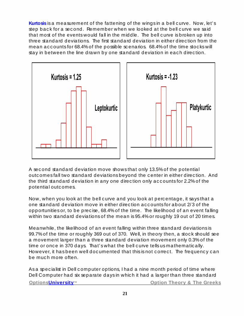
Kurtosis is a measurement of the fattening of the wings in a bell curve. Now, let’s step back for a second. Remember when we looked at the bell curve we said that most of the events would fall in the middle. The bell curve is broken up into three standard deviations. The first standard deviation in either direction from the mean accounts for 68.4% of the possible scenarios. 68.4% of the time stocks will stay in between the line drawn by one standard deviation in each direction.
A second standard deviation move shows that only 13.5% of the potential outcomes fall two standard deviations beyond the center in either direction. And the third standard deviation in any one direction only accounts for 2.2% of the potential outcomes. Now, when you look at the bell curve and you look at percentage, it says that a one standard deviation move in either direction accounts for about 2/3 of the opportunities or, to be precise, 68.4% of the time. The likelihood of an event falling within two standard deviations of the mean is 95.4% or roughly 19 out of 20 times. Meanwhile, the likelihood of an event falling within three standard deviations is 99.7% of the time or roughly 369 out of 370. Well, in theory then, a stock should see a movement larger than a three standard deviation movement only 0.3% of the time or once in 370 days. That’s what the bell curve tells us mathematically. However, it has been well documented that this is not correct. The frequency can be much more often. As a specialist in Dell computer options, I had a nine month period of time where Dell Computer had six separate days in which it had a larger than three standard

OptionsUniversityTM Option Theory & The Greeks
22
deviation one day movement. You heard it right.....six times in a nine- month period! According to the bell curve, that type of event should have happened roughly over nine years not nine months.
What is that saying? That is telling us that our bell curve, the normal distribution, for some reason is not properly accounting for the way stocks deliver returns in reality. Why? We said it earlier. Studies have shown that stock returns are not normally distributed. So, somehow we had to account for all of these additional samples landing outside of three standard deviations. So, what could we do? We fatten up the wings on either side. How do we fatten them up? We fatten up by using kurtosis to show us how.

OptionsUniversityTM Option Theory & The Greeks
23

OptionsUniversityTM Option Theory & The Greeks
24
Now, in order to fatten up or increase the chances of a stock having a more than three standard deviation move, we must increase the percentage chance located in the wings. Increasing the percentage chance in the wings has to affect the percentage chance somewhere else in the bell curve. This is because a bell curve must add up to 100%. There is only a 100% chance of anything happening. So, if we’re going to increase the percentage chance of a more than three standard deviation move, we have to decrease the potential of it doing something else somewhere else. How do we do that? We decrease the percentage chance of the stock either staying in that one standard deviation movement off the mean, decrease the chance of a two standard deviation movement, or some combination of the two. For instance, a three standard deviation to the right is a 2.2% chance, a three standard deviation to the left a 2.2% chance. Those are the numbers. If I want to bump them up to a 5% chance each then I’m going to add a 2.8% chance to each side. That means that I’m increasing the percentage chance of the stock having a three standard deviation move in either direction by 5.6 additional percent. It is impossible to say that a chance of anything happening is 105.6%. So, I have to balance the percent chance to a total of 100%. I’ve got to take away the that additional 5.6% chance from something else. Once I have adjusted the percentage chance to either the one or two standard deviation (or combination of), the total percentage chance of an event is back in line. Now, is this complicated? A bit, however, this is what kurtosis is. This is how kurtosis is used to mutate the bell curve to adjust for the fact that stock returns are log-normally distributed, not normally distributed. It became necessary to take a measure of a stock’s kurtosis and account for it in the pricing of the options. A model was needed to allow for the kurtosis adjustment. The VSK model was developed to do just that. Kurtosis can be calculated and measured historically which will allow for comparison to previous time periods. The VSK model proved to be extraordinary in its pricing of options for stocks that were very volatile. So, for growth stocks that had high volatilities back in the internet crazed days, having a model that understood kurtosis was very important especially for pricing options with longer expirations (out months). Today, any stock
OptionsUniversityTM Option Theory & The Greeks
25
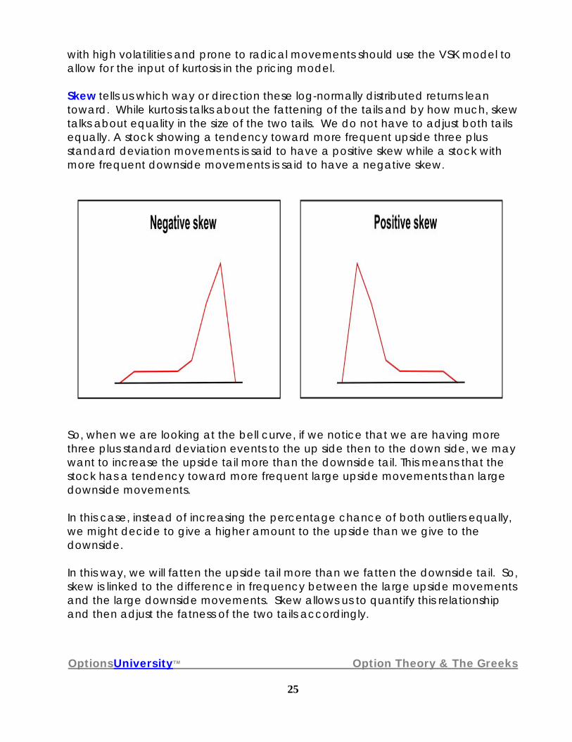
with high volatilities and prone to radical movements should use the VSK model to allow for the input of kurtosis in the pricing model. Skew tells us which way or direction these log-normally distributed returns lean toward. While kurtosis talks about the fattening of the tails and by how much, skew talks about equality in the size of the two tails. We do not have to adjust both tails equally. A stock showing a tendency toward more frequent upside three plus standard deviation movements is said to have a positive skew while a stock with more frequent downside movements is said to have a negative skew.
So, when we are looking at the bell curve, if we notice that we are having more three plus standard deviation events to the up side then to the down side, we may want to increase the upside tail more than the downside tail. This means that the stock has a tendency toward more frequent large upside movements than large downside movements. In this case, instead of increasing the percentage chance of both outliers equally, we might decide to give a higher amount to the upside than we give to the downside. In this way, we will fatten the upside tail more than we fatten the downside tail. So, skew is linked to the difference in frequency between the large upside movements and the large downside movements. Skew allows us to quantify this relationship and then adjust the fatness of the two tails accordingly.

OptionsUniversityTM Option Theory & The Greeks
26
Skew, like kurtosis, can be calculated and measured historically for comparison with previous time periods. So, when you are using a VSK model you can calculate a stock’s historic skew and kurtosis skew to help you determine where they run normally and use this to help determine whether or not the current conditions are high or low. This will help you determine whether the current volatility smile is trading too peaked or too flat. While some of these inputs are weighted more heavily in an option’s price than others, it is critical to realize that they are all important. It is said that you can only get out as good as you put in and this is true with the option-pricing model as well. The better and more accurate your inputs, the better and more accurate your outputs will be.

OptionsUniversityTM Option Theory & The Greeks
27
Pricing Model Outputs – “The Greeks”
As important as the inputs to the model are, maybe even more important, are the outputs, which are commonly known as the “Greeks.” What are the “Greeks?” A Greek is a measure of an option’s sensitivity to a certain variable. There are several different types of Greeks, some a little more popular, some better known, and some more important than others. The Greeks are our risk measurement tool. Let us identify some of the Greeks. First, we have Delta that is known as the first derivative. Delta tells us how much an options price will change with a movement in the underlying stock price. Next, we have Gamma. Gamma is the second derivative and is considered the delta of the delta. Gamma tells us how much the option’s delta will change with a one-dollar movement in the stock. Theta means time decay and tells us the rate at which an option’s price will decay on a daily basis. Also, there is Vega that tells the option’s price change in relation to a one-tick movement in volatility. Vega is a measure of the option’s volatility sensitivity. Finally, Roe measures interest rate sensitivity. It tells you the change in the option’s price in relation to a movement in interest rates.

OptionsUniversityTM Option Theory & The Greeks
28
Delta
Delta, the first of our Greeks, is considered the first derivative because it is the first step off of the stock. Although delta has several different definitions, in general, delta explains or measures for us, the price movement of an option with a one-dollar movement in the stock. That is the generic description. Delta has a total of three definitions that are all important. Delta - percent change As stated above, delta tells us how much an option’s price will change per a one-dollar movement in the stock. For example, if we are looking at a fifty-delta option and the stock moves a dollar, the option should move fifty cents. If we are looking at a thirty-delta option, and the stock moves one dollar, we are looking at a thirty-cent move. This movement demonstrates Delta’s definition of percent change. Delta describes the percent the option price moves with a stock price move. A forty-Delta option will move forty percent of what the stock just moved. That is percent change. A sixty-delta option will move sixty percent of what the stock just moved. Delta –percent chance Delta is also defined as percent chance. A fifty-delta option has a fifty percent chance of finishing in-the-money. A thirty-delta option has a thirty percent chance of finishing in-the-money. A ten-delta option will have a ten percent chance of finishing in the money and so on. Delta- hedge ratio Delta’s last definition is that of hedge ratio. Remember we talked about options being the perfect hedge. If we were long 800 shares of stock (or 800 deltas as each share of stock is equal to one delta), and wanted to hedge our position, we know we could sell some calls to hedge that position. The question is - how many calls? We could do it one-for-one. If we did that, we would still be long delta. On the other hand, we could sell enough deltas through the calls to perfectly hedge the delta risk of our stock. The answer is in delta’s definition of hedge ratio. Hedge ratio tells us how many calls we need to sell to become delta neutral. Say we were looking at a 40 delta call.
OptionsUniversityTM Option Theory & The Greeks
29
The 800 long delta position from the stock, divided by the 40 deltas of the call will equal 20. That is how many calls we would need to sell – 20. Thus, if we sold 20 of the 40 delta calls, we would have short 800 deltas that would perfectly hedge our long 800 deltas from the stock. We can also use puts to hedge our long stock delta. If we were long 800 shares of stock and we were looking at a fifty-delta put, we would buy 16 of them. Why? Because the fifty deltas of the puts, multiplied by 16 puts, will give us short 800. The short 800 total deltas from the 16 puts will perfectly hedge the long 800 deltas from our long 800 share stock position. Make sense? It also works the other way. If we bought a 40 delta call and we bought ten of them, we would have 400 long deltas. In order to delta hedge our position we should sell 400 shares of stock. Selling 400 shares of stock will perfectly hedge our long 400 delta position from the long calls Delta has three definitions: percent chance, percent change and hedge ratio. All of equal importance: no one ahead of the other. Delta of Calls Let us talk about the delta of calls. First, calls are a long instrument so calls have long deltas. Obviously, calls with different strike prices and different expiration months will have different deltas. When trading calls, buyers of calls acquire long delta positions while sellers of calls acquire short delta positions. It is important to remember that call deltas are positive. Any call, whose strike price is lower than the current stock price, is considered to be an in-the-money (ITM) call and will have a delta above sixty. The deeper in-the-money you go, or the lower price strike price you look at, the higher the deltas will be until they finally approach a hundred. Any call whose strike price is equal to or close to the current stock price, is known as an at-the-money (ATM) call, and will have deltas right around fifty. Any call, whose strike price is higher than the current stock price is said to be an out-of-the-money (OTM) call and have deltas less than forty. The further out-of-the-money you go, the lower the deltas will be until finally reaching 0.
OptionsUniversityTM Option Theory & The Greeks
30
Delta of Puts Now, let us talk about the delta of puts. First, puts are a short instrument so puts have short deltas. Obviously, puts with different strike prices and different expiration months will have different deltas. When trading puts, buyers of puts acquire short delta positions while sellers of puts acquire long delta positions. It is important to remember that put deltas are negative. Any put, whose strike price is higher than the current stock price, is considered to be an in-the-money (ITM) put and will have a delta above sixty. The deeper in-the-money you go, or the higher priced strike price you look at, the higher the deltas will be until they finally approach a hundred. Any put, whose strike price is equal to or close to the current stock price is known as an at-the-money (ATM) put and will have deltas right around fifty. Any put, whose strike price is higher than the current stock price is said to be an out-of-the-money (OTM) put and have deltas less than forty. The further out-of-the-money you go, the lower the deltas will be until finally reaching 0. The Delta Connection There is an extremely important delta connection that exists between a call and its corresponding put. First, what does corresponding mean? Corresponding refers to two options, one a put, the other a call, in the same month with the same strike price. For instance, the January 20 call’s corresponding put is the January 20 put. The May 90 call’s corresponding put is the May 90 put. The corresponding call of the July 60 put is the July 60 call. The important thing to know here is that when looking at the deltas of a call and its corresponding put, the sum of the absolute value of a call plus its corresponding put must equal one hundred. Key Point: The absolute value of a call and its corresponding put deltas must equal one hundred. Let us try a few samples to see how that works. What we have here is a Delta chart. These are actual deltas that were taken directly from real trading sheets. We will look to see if the absolute value of a call and its corresponding put will equal a hundred. Look at the July 65 calls with a Delta of +56. Now look at the put. The July 65 put delta is -44. Absolute value of minus 44 is 44. 56 plus 44 is 100.

OptionsUniversityTM Option Theory & The Greeks
31
Try another one. Look at the July 75 calls. The July 75 calls are a +12 Delta. The July 75 puts are a -88 delta. The absolute value of -88 is actually 88. Eighty-eight plus 12 equals 100. Do another one. Look at the October 60 put. The October 60 put is a -28 delta. Its absolute value is 28 deltas. The October 60 call have a +72 delta. The absolute value of 72 added to the absolute value of 28 equals 100. As you see, this works every time. Position Delta Position delta is defined as the total delta of your position. It is calculated as the sum of all the deltas of the stock position, plus the deltas of all the calls and all of the puts in that single stock. As a floor trader, you would have many strikes where you were long twenty calls and short fifteen puts. This strike, you were long a hundred calls. That strike, you were short forty puts. And, this other strike, you were long a hundred puts. The puts and calls are all over the board. When we talk about position delta, we take a net total of all the deltas of the puts, of all the deltas of the calls, and all the delta we have in the stock and add them together. When we do that, it will give us one number, one delta number plus or minus and that is our position delta. Position delta tells us that if our overall position is long a thousand deltas and the stock goes up a dollar, we will make one thousand dollars. If we are long one thousand deltas, and the stock goes up fifty cents, we will make five hundred dollars. If we are short five hundred deltas and the stock goes up a dollar, we will lose five hundred dollars. If we are short a thousand deltas, and the stock goes up a dollar, we will lose one thousand dollars. That is what position delta is and what it tells us. Delta Neutral Now, you may create a position that has no delta, a position called Delta Neutral. That means you have eliminated your position’s sensitivity to stock movement. You might wonder how you will make money doing that. Remember, options allow you to make money in many more ways than a stock does. You might have an opportunity to try to collect decay. In the course of doing that, you do not want to double your bet by having a delta position on also.

OptionsUniversityTM Option Theory & The Greeks
32
Therefore, you neutralize your delta, become delta neutral and just play your decay. Or, you might have a volatility position on. You might be making a bet that volatility is going to go up or go down. If so, you would hate to double down on that bet by having a delta position that can work against your volatility position, so you will eliminate your delta position by becoming delta neutral. That way, if the stock goes up, or if the stock goes down, it does not matter. Your focus is on whether volatility goes up or down without the worry of a delta position. Delta Graph Take a look at a Delta graph seen below. There is one here for you to look at. These are the deltas of the calls that I took off your trading sheets with a stock price of $65.50 and a 30 volatility. Lesson: Trading Sheet #1 These are from Trading Sheet Number 1 located in the appendix. I made a graph of the information from that sheet. I put the months across the top, and put the strike prices down the side, then filled in all the deltas for each option. We will use this graph to observe the effect of time on delta or trumpification.
DELTA CHARTCALLS STOCK PRICE 65.50 30 VOL.
26184080
352813375
4641301870
5857565665
7072819160
81859510055
90949910050
JanuaryOctoberJulyJuneStrike Price

OptionsUniversityTM Option Theory & The Greeks
33
First, observe the vertical look of delta in these calls. What I mean by that is, just look at June. As you can see, with the stock price at $65.50, you have some strikes, (the fifties, the fifty-fives and the sixties) that are in-the-money. The sixty-fives are at-the-money, and the seventies, seventy-fives and eighties are out-of-the-money. We previously said that any in-the-money option will have a delta approaching a hundred – or at least- higher than sixty, which the fifties, the fifty-fives and the sixties do. You can see that as you go deeper in-the-money, or lower in strike price, the deltas increase. Our at-the-money was going to have a delta of fifty or so, which our sixty-fives do. Our out-of-the-money options were going to have deltas less than fifty and those deltas would decrease as we go further out-of-the-money, meaning up higher in strike prices, which the seventy-fives and eighties do. Our graph supports the theory of the delta of calls. Time Effect on Delta Now, look at the range between the June 50 call’s delta and the June 80 call’s delta. We have a delta in that range of as high as a hundred and a delta as low as zero for a range of 100. Now, we go out a month and look at our July options. Our range has tightened. Our range goes from a high of ninety-nine to a low of four. Now, go out to October. Our range has tightened even more from a high of ninety-four to a low of eighteen. Finally, out in January and our range is even tighter, from a high of ninety to a low of twenty-six. From repeated observations, we can form a hypothesis. That is, that as we go out over time, the ranges of our deltas are going to crunch in toward 50 as they do here. Let us examine that affect a little closer. First, look at the in-the-money calls. The 55 strike is in-the-money and will suit our purposes. In June, the June 55 calls are a hundred deltas. The July 55’s are 95 delta, obviously less than the June. The October 55’s are 85 delta, even less than the July. Finally, the January 55 calls delta is even less than October’s. So what do we learn? We learn that as you go out over time, the Deltas of in-the-money calls decrease. Now, look at the at-the-money options. Check the sixty-five strike, which is the at-the-money option with the stock at $65.50. The June 65’s are 56 delta. The July 65’s are 56 delta. The October 65’s are 57 delta. The January 65’s are 58 delta.

OptionsUniversityTM Option Theory & The Greeks
34
What do we notice here? We notice that as we go out over time, the deltas of the at-the-money calls hold steady. Over time, the in-the-money calls are decreasing, while the at-the-money calls are holding steady. Finally, look at some out-of-the-money calls. The June 75 calls, have 3 delta. The July 75 calls are an increase over the June’s at a 13 delta. The October 75 calls are an increase over that at 28 delta. Even higher, the January 75 calls are 35 delta. So what can we say? As we go out over time, the deltas of out-of-the-money calls increase. As we look out over time, we see the in-the-money call deltas decreasing (pushing down toward 50); we see the delta of the out-of-the-money calls increasing, (pushing up toward 50); and we see the delta of the at-the-money calls holding steady at around 50. This “crunch” of deltas approaching 50 looking out over time is called trumpification. Trumpification is defined as a delta effect caused by time and/or volatility movement in which the deltas of in-the-money options decrease toward 50, out-of-the-money options’ deltas increase toward 50 while the at-the-money options’ deltas hold steady around 50. The importance of trumpification is to see how an option’s delta changes as the option approaches expiration.

OptionsUniversityTM Option Theory & The Greeks
35
Trumpification affects both the calls and the puts in the same manner. In the above description of the trumpification effect, we observed the effect by first looking at the present, then out into the future noticing the changes. But, in order to use trumpification’s effect to help us understand and anticipate what will happen to the delta of our option as expiration approaches, we must view it in reverse. Let’s change our perspective by first looking out in the future and seeing what happens as we span back into the present. This can be done by simply looking at the chart from right to left instead of left to right. In this way, we can observe the change in delta as expiration draws near. We have to understand that as an owner, or as a short holder of the in-the-money options, deltas are going to increase (calls get longer, puts get shorter) as expiration gets closer. Remember, as we looked out over time, the deltas of in-the-money options decrease, but as time passes and they come closer to us, they are increasing. The at-the-money options hold steady. The out-of-the-money options, when we look out over time, increase, but as time goes by and expiration gets closer, they decrease. That is important since at some time that is going to affect our delta Position. We will see our delta position changing as days go by. We are going to wonder why that is happening. Now we know that this is happening because of the effect known as trumpification. If you drew a graph of this chart, with all the deltas, you would have this real wide range up front as seen in the month of June.. As you moved out over time, the deltas would decrease a little bit in the upper section, the in-the-money calls, but meanwhile, as you moved out over time, the deltas would increase a bit in the out-of-the-money calls with the middle staying still. Every month that would happen more and more, constantly and progressively. Everything would push tighter and tighter the further out you go. And sure enough, when you do your homework and make a graph of this like you should, you will notice that you are looking at a trumpet shaped graph. That is how trumpification got its name. As stated, trumpification works the same way on puts. Look at your put chart below. Look at the seventy-five strike and go out over time. These in-the-money puts lose delta as we go out over time. The out-of-the-money puts, like the fifty-five

OptionsUniversityTM Option Theory & The Greeks
36
strike, gain deltas, have bigger deltas as you go out over time. The at-the-money strike, the sixty-five, stays relatively flat. There is no increase or decrease in the delta. So, yes, trumpification works for the puts too. You will see that when you make a chart, then graph it, and the graph takes the shape of a trumpet.
DELTA CHARTPUTS STOCK PRICE 65.50 30 VOL
-76-84-98-10080
-66-73-88-9875
-55-59-70-8270
-43-44-44-4465
-30-28-19-960
-19-15-5055
-10-6-1050
JanuaryOctoberJulyJuneStrike Price
Delta and Volatility Now, back to delta. We saw the effect of the movements of stock and the movement of time: but what about the effect of volatility? Remember that time movement created the effect called trumpification. The definition of trumpification is the effect on delta caused by time and/or volatility that increases the deltas of out-of-the-money options, and decreases the deltas of in-the-money options, pushing them all toward fifty. So, by definition, we should be able to see this effect with a change in volatility.
OptionsUniversityTM Option Theory & The Greeks
37
DELTA CHARTCALLS STOCK PRICE 65.50 70 VOL
.
4942261280
5347352375
5854463770
6360575565
6867697460
7374798855
7880889650
JanuaryOctoberJulyJuneStrike Price
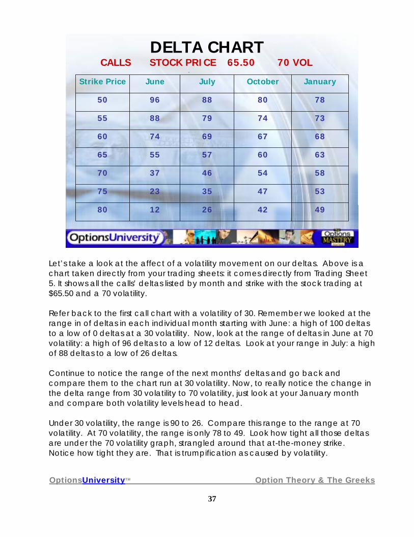
Let’s take a look at the affect of a volatility movement on our deltas. Above is a chart taken directly from your trading sheets: it comes directly from Trading Sheet 5. It shows all the calls’ deltas listed by month and strike with the stock trading at $65.50 and a 70 volatility. Refer back to the first call chart with a volatility of 30. Remember we looked at the range in of deltas in each individual month starting with June: a high of 100 deltas to a low of 0 deltas at a 30 volatility. Now, look at the range of deltas in June at 70 volatility: a high of 96 deltas to a low of 12 deltas. Look at your range in July: a high of 88 deltas to a low of 26 deltas. Continue to notice the range of the next months’ deltas and go back and compare them to the chart run at 30 volatility. Now, to really notice the change in the delta range from 30 volatility to 70 volatility, just look at your January month and compare both volatility levels head to head. Under 30 volatility, the range is 90 to 26. Compare this range to the range at 70 volatility. At 70 volatility, the range is only 78 to 49. Look how tight all those deltas are under the 70 volatility graph, strangled around that at-the-money strike. Notice how tight they are. That is trumpification as caused by volatility.

OptionsUniversityTM Option Theory & The Greeks
38
So, why do you want to know trumpification? Easy, because if you understand trumpification, you understand how time and volatility affect the deltas of your option positions. For instance, say you were long some in-the-money calls and somebody says, “Hey, volatility was up pretty big today in your stock.” You will know immediately that your overall delta position has decreased because of trumpification. You will have been prepared for this because you know that trumpification affects the in-the-money calls by decreasing their deltas. Although you can not control the changing of the delta due to the movement of volatility, you will have been prepared for the possibility and not surprised by it. So, right off the bat, you already have a better understanding of your position because you know what is going to happen to your deltas. Depending on where your option deltas are located (in-the-money, at-the-money, or out-of-the-money) you’ll know what a volatility’s increase will do to your position as well as what a volatility decrease will do. Here lies the importance of understanding trumpification.....knowing how your overall delta position will change with changes in volatility and the movement of time. For a little side work, take your trading sheets, take your notes, and look at the different things we just discussed. Go to the delta charts and get the delta values under each volatility level and graph them. See the trumpet shape the graph will take on. Take a look at deltas of calls and puts when volatility is 70 and see what happens to them when you move volatility down to 30. Go back and forth visualizing this and seeing that. Work the numbers of the absolute values of the calls and their corresponding puts and check that their sum actually equals 100 each and every time. Go over as many examples as possible to solidify the concepts of delta because those concepts will repeat themselves over and over as our discussion of options continues into strategies.

OptionsUniversityTM Option Theory & The Greeks
39
Gamma
Next, we’re going to take a look at Gamma. Gamma is the second derivative. Delta measures how much an option’s price changes with a movement in the stock. Gamma, in turn, measures how much the delta changes with a movement in the price of the stock. Remember, deltas are not fixed. Deltas are determined by where the stock is, and as the stock moves, deltas move.
How do we quantify the amount by which our deltas are going to change? Gamma tells us the amount. The thing to remember about gamma is that it is the delta of the delta. It measures how much the delta changes with a movement in the stock. Therefore, it has the title, the second derivative.
Obviously, delta and gamma are connected. However, they are not connected
in a very important way.....calculation. Delta is calculated for each and every different individual call and put. But, gamma is different. Gamma is calculated by strike price. Gamma does not differentiate between calls and puts. It only focuses on strike price. Gamma knows the strike, not the call or put of that strike. It does not acknowledge the difference between the August 50 call and the August 50 put. It views them both the same – the August 50 strike. This means that corresponding calls and puts have the same, identical gamma value. This is a very important concept for later. There are two types of gamma. There is long gamma and there is short gamma. How do you acquire gamma? Any time you buy an option, any option, whether it is a call or a put you obtain long gamma. Any time you sell an option, call or put, you obtain short gamma. Simply stated, you obtain long gamma by buying an option; you obtain short gamma by selling an option. Time affects gamma. What do we mean by that? What we mean is that gamma increases as expiration approaches. As time goes by, an option’s gamma value increases because gamma is highest in the front month at-the-money. Let us take a look at that.

OptionsUniversityTM Option Theory & The Greeks
40
GAMMA CHART
2.12.31.8.480
2.32.93.72.875
2.43.25.27.770
2.33.05.07.265
2.02.42.81.860
1.51.5.8.155
.9.7.1050
JanuaryOctoberJulyJuneStrike Price
Look at the above gamma chart. These gamma values are taken straight from your trading sheets. These are the calculated gammas values with the stock at $67.50 and a volatility of 30. Both the 65 and 70 strikes are roughly at-the-money. As we look at the month of June and we look vertically at gamma, we see that gamma is the highest when it is at-the-money. The 65 and 70 strikes have the highest gamma. The gamma values decrease as you move away from the at-the-money strikes in either direction. We have identified the 65 and 70 as at-the-money. Look up at the 60 strike. You will see a decrease in the gamma value from the 65 and 70 strikes. Now, look at the 55 strike and you will notice even more of a decrease. Let us turn our attention to the upside. Taking notice of the June 75’s gamma value, we see that it is lower than the 70 strike gamma value. Continuing our investigation of the upside, the June 80 gamma value is even lower than that. So, when we’re looking at gamma vertically, that is in a single month, we must remember that gamma is the highest at-the-money and decreases as we move away from the at-the-money in either direction, whether we go further in-the-money or further out-of-the-money. Key Point: In either direction, gamma values decrease away from its highest point, which is located at-the-money.

OptionsUniversityTM Option Theory & The Greeks
41
Now, how does gamma behave over time? Let us look at Gamma in a horizontal
or out over the months at the same strike price. First, let’s look at the 70 strike. The June 70 strike gamma value is 7.7. Meanwhile, the July 70 gamma value is 5.2 which is less than the June 70 gamma value. The October 70 gamma value is even less than the July gamma. Finally, the progression continues into January where the gamma value is the lowest of any of the months.
Take another strike as an example. Look at the 65 strike from month to month and
compare the results. In June, the gamma value of the 70 strike is 7.2. It decreases in July to 5.0 and decreases even further to a 3.0 gamma value in October. It has even more of a drop out in January. As you can see, the gamma decreases when we look at it horizontally, that is, at a single, specific strike out across time. The lesson learned from this observation is that gamma is highest front month, at-the-money. Now, you may notice something odd when looking at this chart. You might notice that the June 50 gammas value is lower than the January 50 gammas. As you can see, it is miniscule but it is true. That is because the January 50 calls are so deep in-the-money they are acting like stock, and stock does not have gamma. When you talk about very deep in-the-money options, you might actually see an increase in gamma values over time. You see it a little in the 55 strike also. Why? Because in the front months, the very deep in-the-money options are trading at parity to the stock. Parity, as you know, means equal to. These options trade at parity because there is so little time left until expiration. These options are so far deep in-the-money that the pricing model feels the current implied volatility of the stock is not enough to threaten that the strike will not finish in-the-money by expiration. In July, there is more time, so the July 55 strike is a little more of an option (not as high a delta) than the June 55 strike. Thus, the July 55 strikes have a little more gamma. The same exception holds when you get way out-of-the-money. When you get way out-of-the-money, like in the 80 strike, these options are valueless. They are so far out-of-the-money that the option model is saying that under the current volatility and with such little time left, there is no way for that option to finish in-the-money by expiration. They are no longer a viable option. They are worthless. If it is worthless and it’s not an option, it can’t have gamma. Now, the July 80’s have a little more time left before expiration. Because they

OptionsUniversityTM Option Theory & The Greeks
42
have a little more time, they are a little more of an option. They still have a chance. Thus, have a little more gamma. When you are looking at the deep in-the-moneys and the way out-of-the-moneys and you’re looking at them horizontally, you will notice the gamma will probably increase slightly out over those times. However, the rule of thumb is gamma is highest front month at-the-money and decreases when you move vertically in either direction away from the strike, and decreases out over time except for deep in-the-money options and way out-of-the-money options. Like delta, gamma can have a position effect also. What we mean by that is that there is a gamma for every single different option strike. If you have a position of multiple options series under the same stock, each one of those options will be subtracting from or adding to the gamma of the total position. So, if you took a net option position for each strike under an individual stock, and multiplied it by the gamma of the strike, you would then get a gamma position for each strike price in which you have open contracts. From there, you can add together all the gammas from all the different strikes to give you a total position gamma. The two types of gamma, long and short, affect your delta position differently. A fallacy that exists in some traders’ minds is that long gamma is good gamma and short gamma is bad gamma. This perception is totally untrue. Gamma is neither a good nor bad thing. It is simply long or short. You must be able to apply or trade both long and short gamma just as easily because different conditions require different types of gamma positions. Some feel that long gamma is easier to trade and it normally is. However, we know that selling options is the right side of the trade between 75-80 percent of the time, so being comfortable with trading short gamma is very important. It is important to favor neither and know both equally well.

OptionsUniversityTM Option Theory & The Greeks
43
Long Gamma Trading
First, let’s talk about long gamma and how it affects your delta position. When you are long gamma, and the stock increases in value, your delta position increases by the amount of your gamma position per one dollar move in the stock.
If the stock were to go down, your delta position would decrease by the amount
of your gamma position per one dollar movement in the stock. Simply put, if the stock went up, and you were long gamma, your delta would increase. If the stock went down and you were long gamma, your delta would decrease. Why is that? Can we see if that really happens? Lesson – Trading Sheet #1 Let’s grab Trading Sheet Number 1 from the appendix and look at a little example. With the stock at $65.50, we will buy the June 65 call. Now, as we know when we buy an option, we acquire long gamma. We are doing this to see whether we actually acquire a larger delta position when the stock goes up while we are long gamma. Let’s see if that happens and how it happens.

OptionsUniversityTM Option Theory & The Greeks
44
When we buy the June 65 calls with the stock at $65.50, the theoretical value is $2.04 with a delta of 56. Now, we know that with an upward stock movement, the delta will increase by the amount of our gamma per a one dollar movement in stock. In order to better view the gamma affect, we are going to do a delta neutral trade. We will buy 10 of the June 65 calls at 56 deltas each. Fifty-six deltas times our 10 contracts is 560 deltas. In our position thus far, we are long 560 deltas through calls. In order to neutralize or flatten our delta position, we sell 560 shares of stock. That will neutralize our delta to exactly zero. We now have no delta in our position. We are long 10 calls (10 calls, at 56 Deltas each, equal long 560 deltas) and we are short 560 Deltas in stock. We are now delta neutral. Now, observe what happens when the stock goes up on your trading sheet. When the stock moves from $65.50 to $69.50, the delta of the call position increases. At our example’s starting point, with the stock at $65.50, the calls were 56 deltas. Now that the stock is up at $69.50, the calls are now 85 deltas. Since we are long 10 of them, the position is now long 850 deltas through the calls. But, we are still short only 560 shares of stock. The position is no longer delta neutral anymore. It is long delta. How long? Well, the position is now long 850 deltas in the call position and short 560 deltas in the stock position for a total of 290 long deltas. Our delta position started out as flat and is now long 290 deltas from gamma’s effect with the movement of the stock. So, with the stock going up, our long gamma position increased our delta position. Using the same example, let’s look at what happens when the stock goes down. We will move the stock from $65.50 down to $61.50. The stock deltas are going to be the same, short 560. But again, the option deltas have changed. The delta of the options, the June 65 calls, went from 56 down to 23. They lost 33 Deltas. The overall delta position in the calls is no longer long 560. It is now only long 230. And, if that is so, then the overall delta of the position is now short 330 deltas (short 560 from stock, long 230 from calls). A position that started as delta neutral is now short 330 deltas due to gamma. As evidenced in the example, when you are long gamma and the stock goes down, your delta position decreases.

OptionsUniversityTM Option Theory & The Greeks
45
Now let us talk about short gamma. Short gamma works the opposite way from long gamma. If you are short gamma and the stock goes up, your delta position would decrease. If you were short gamma and the stock goes down, your delta position would increase.
Short Gamma Trading
To see this, we will use the same example as above but this time, instead of buying calls (creating a long gamma position) we will sell the calls (creating a short gamma position). So, we sell the July 65 calls at 56 deltas and become short 560 deltas in our call position. To offset that, we will buy 560 shares of stock. Our position now is long 560 shares of stock and short 10 of the June 65 calls at 56 deltas each. This will give us an overall position delta of zero or delta neutral. Again we are delta neutral here, but because we are short the calls, we are short gamma. Now, let’s see what happens when the stock goes up. As before, with the stock price of $65.50, the June 65 calls are 56 deltas. Now, take the stock price up to $69.50 on your sheets. Look at the new delta of the June 65 calls.

OptionsUniversityTM Option Theory & The Greeks
46
Those June 65 calls are going to be 85 deltas. So, where the delta in our stock, long 560, remains constant, the delta in the call position has changed thus changing the overall position delta. The delta in the calls increased from 56 up to 85. Our short call position is now creating a short 850 delta position. We are still long 560 deltas from the stock position, giving us now a total position of short 290 deltas. Our delta position went from flat to a delta position of short 290 due to the position’s gamma. We see that, with short gammas, as the stock goes up, you get shorter delta. Key Point: With short gamma, as the stock goes up, you get shorter delta. Again, let’s go back to our original example where we were looking at the June 65 calls with the stock at $65.60 and 56 deltas. As before, we are going to sell 10 of the June 65 calls, which we said would give a negative 560 delta. We were going to buy 560 deltas by purchasing 560 shares of stock, giving us a flat delta position. Our position delta is flat. We sold the calls so we know we are short gamma. Now, we said that if a stock goes down when you’re short gamma, you acquire more long deltas. Let’s see if that’s true. It worked in the other direction, so let’s check out this direction. Going back to the example we have been working with, let’s move the stock price down to $61.50. With the stock price at $61.50, the delta of the June 65 calls is no longer 56, it is now 23 and we are short 10 of them giving us a net short delta in our call position of short 230 deltas. Our stock position though remains the same at long 560 deltas because of our long 560 shares. 560 long deltas in the stock, and 230 short deltas in the calls, results in an overall total position of 330 long deltas. We were flat delta with the stock at $65.60 and now we are now long 330 deltas down at $61.50 due to our gamma position. Just like the formula stated, if you are short gamma and the stock goes down, you acquire long deltas. You have your trading sheets. Try a few practice runs like we did in our examples above. Make sure that you are fully comfortable with both the long gamma affect on delta as well as the short gamma affect on delta. Make sure you understand both equally well and always remember, there is no good gamma, and there is no bad gamma. There is only long gamma and short gamma, and both will make you money in the right situation.
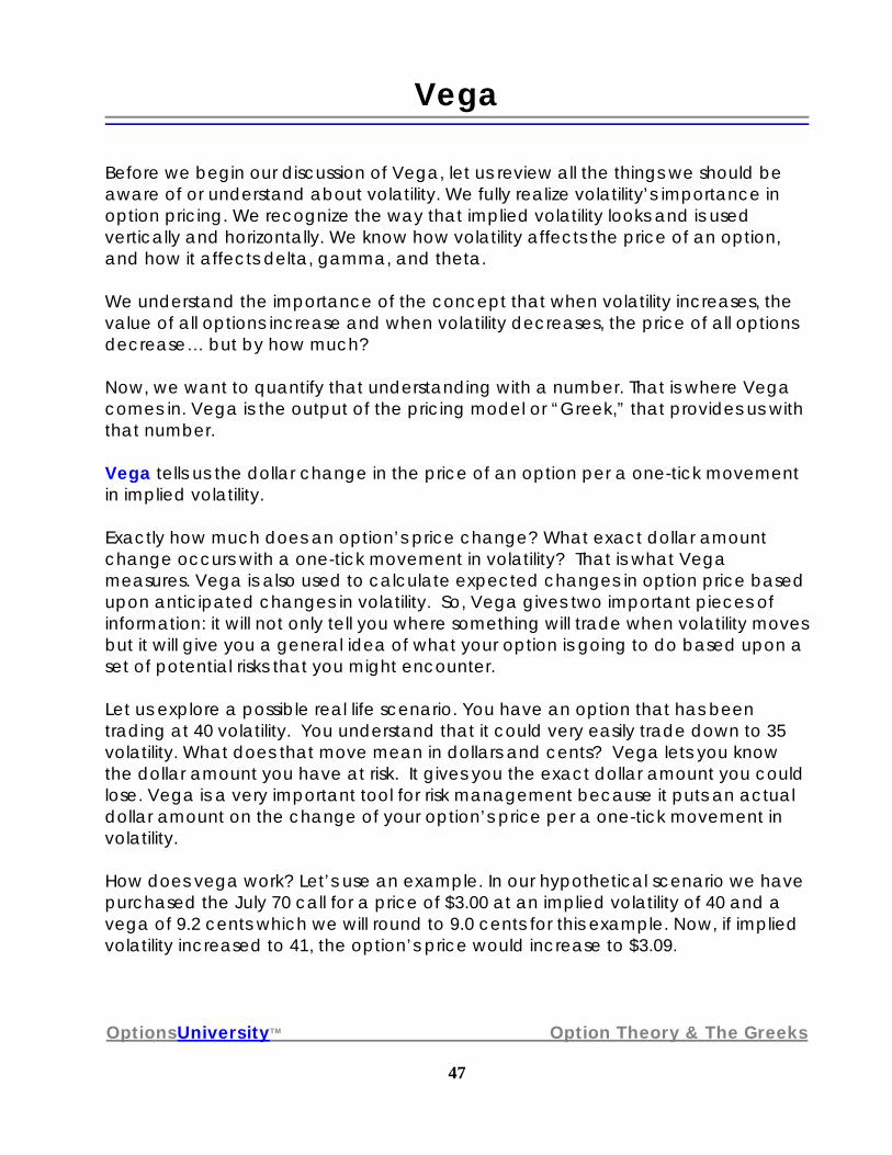
OptionsUniversityTM Option Theory & The Greeks
47
Vega
Before we begin our discussion of Vega, let us review all the things we should be aware of or understand about volatility. We fully realize volatility’s importance in option pricing. We recognize the way that implied volatility looks and is used vertically and horizontally. We know how volatility affects the price of an option, and how it affects delta, gamma, and theta. We understand the importance of the concept that when volatility increases, the value of all options increase and when volatility decreases, the price of all options decrease… but by how much? Now, we want to quantify that understanding with a number. That is where Vega comes in. Vega is the output of the pricing model or “Greek,” that provides us with that number. Vega tells us the dollar change in the price of an option per a one-tick movement in implied volatility. Exactly how much does an option’s price change? What exact dollar amount change occurs with a one-tick movement in volatility? That is what Vega measures. Vega is also used to calculate expected changes in option price based upon anticipated changes in volatility. So, Vega gives two important pieces of information: it will not only tell you where something will trade when volatility moves but it will give you a general idea of what your option is going to do based upon a set of potential risks that you might encounter. Let us explore a possible real life scenario. You have an option that has been trading at 40 volatility. You understand that it could very easily trade down to 35 volatility. What does that move mean in dollars and cents? Vega lets you know the dollar amount you have at risk. It gives you the exact dollar amount you could lose. Vega is a very important tool for risk management because it puts an actual dollar amount on the change of your option’s price per a one-tick movement in volatility. How does vega work? Let’s use an example. In our hypothetical scenario we have purchased the July 70 call for a price of $3.00 at an implied volatility of 40 and a vega of 9.2 cents which we will round to 9.0 cents for this example. Now, if implied volatility increased to 41, the option’s price would increase to $3.09.

OptionsUniversityTM Option Theory & The Greeks
48
Remember, vega measures the change in an options price per a one-tick movement in volatility. So, with volatility increasing one tick to 41, the option will increase in value by 9 cents. If implied volatility were to decrease one tick down to 39, the price of the option will decrease by 9 cents for a new value of $2.91. It is important to realize that movements in implied volatility are not restricted to just one tick at a time. In order to calculate an implied volatility movement of more than one tick, you simply calculate the difference between where implied volatility is and where it was. Next, take that difference and multiply it by the option vega. Then add or subtract that amount to the old theoretical value to create the new theoretical value. For instance, recall the particulars of our previous example: the July 70 call is worth $3.00 at 40 volatility with a vega of 9 cents. If implied volatility were to increase five ticks to 45 volatility, you could calculate the new theoretical value at this new volatility level (45). First, note that there is a five-tick volatility difference (original 40, new 45). Take that five-tick difference and multiply it by the 9 cent vega. This equals $0.45 (5 times .09). Now add this to the original theoretical value of $3.00 and you come up with a new theoretical value of $3.45 at an implied volatility of 45. Remember, if volatility were to decrease instead of increase, we would use the same calculation except we would subtract from our original theoretical value instead of add to it. So, in our previous example, if the volatility decreased five ticks down to 35 volatility, we would still multiply the vega (.09) by the change in volatility which is five ticks (40-35) and that will again equal 45 cents. This time however, we are dealing with a decrease in volatility so we will subtract these 45 cents from $3.00 giving us a value of $2.55. This will be the new theoretical value of the July 70 call at 35 volatility. As a rule of thumb, if we are looking at an increase in volatility, we will be increasing the value of the option. If we are looking at a decrease in volatility, then we will be decreasing the value of the option. Using this concept, we can also calculate the volatility in regards to a change in theoretical value. The previous few paragraphs showed you how to use vega to determine the new theoretical value of an option with a set and known volatility change. Now, we will use vega to determine the implied volatility level at which an option is trading. Again, there is a formula to follow for this calculation. Using our previous example once more, we first take the difference in the two theoretical values. The original theoretical value in our scenario was $3.00, which we know to be 40 volatility.

OptionsUniversityTM Option Theory & The Greeks
49
Let’s say that the July 70 call is now trading at $3.18 (all other things being equal) which is an increase in price. The difference in price is 18 cents. We take this difference ($0.18) and divide it by the options vega ($.09) to solve for volatility. When we do this, we come up with two volatility ticks. We now take those two ticks and add them to our old or original implied volatility of 40. Since we are looking at an increase in option price, we know we must be dealing with an increase in implied volatility. From our calculation, we know we are dealing with a two-tick increase in the implied volatility. With the option now trading at $3.18, the new implied volatility level must be 42. We know that the price of options can decrease as well as increase. So, in a situation where the option price decreases below the original theoretical value ($3.00 in this case), we use the same calculation method used above to find the volatility level except we would subtract the volatility ticks from our original volatility. Now you will have noticed in the course of our discussions the repetition of certain points. You will notice as we cover volatility and Vega that repetition will happen even more and you might ask, “Why does he keep repeating himself?” I am trying to emphasize the most important concepts about the topic! When I was teaching option theory on the floor of the exchange, I told my students that anytime there was a question, whether verbal in class or written on a test, that involved volatility or vega as part of the answer they should underline and capitalize every letter of the words volatility or vega. What I was trying to do then for them, as I am trying to do now for you is to emphasize the importance of volatility and vega in options. Vega’s importance is huge. If volatility is part of a three, four, five-part answer in a test, it should be listed first, every letter capitalized and underlined; that is how important volatility is to options. Volatility is what separates the option product from all the other products. What separates option from stock is that you can trade the volatility. Let’s take a look, a closer look at Vega to see how it works.

OptionsUniversityTM Option Theory & The Greeks
50
VEGA CHART
.186.120.030.00380
.207.149.063.01875
.215.164.092.05370
.205.156.087.05065
.174.123 .047.01160
.129.076.013055
.080.035.001050
JanuaryOctoberJulyJuneStrike Price
Here is a vega chart. Vega’s are a dollar amount in cents, so when you see something that has a five vega, it means a five cent vega. Take a look at the month of July and focus on the 70 strike. The 70 strike is roughly at the money. In fact, both the 65 and 70 strikes are roughly at the money because the stock is located in between the two at $67.50. We see that the 65 and 70 strike vega prices are very similar. However, when we move down in strike, but still looking at July, we see that the July 60 vega is less than the July 65 and 70 strikes and we see that the July 55 vega is even less than the July 60 vega. Looking in the other direction, looking toward the higher strikes, we see that the July 75 vega is lower than the July 65 and 70 strike vega’s. The July 80 strike vega is even lower than the July 75 strike vega. When observing vega’s behavior vertically along all the strikes in the same month, in the same way as when we viewed gamma, vega is highest at the money and decreases as you move away from the at-the-money strike in either direction. Let me say that again; vega is highest at-the-money and it decreases as you move away from the at-the-money strike in either direction. That is vega’s vertical look; highest at-the-money, decreasing as we move in either direction away from the at-the-money strike. In its vertical look, vega is similar to gamma in appearance. Remember, gamma is also highest at-the-money and as

OptionsUniversityTM Option Theory & The Greeks
51
you move away from the at-the-money strike in either direction gamma decreases. However, there is a difference between vega and gamma when viewed on the charts. We see it when we look at vega horizontally, or across the same strike from month to month. Remember we spoke about gamma being highest in the front month and decreasing as we went out over time. Vega presents the opposite picture; vega increases as we go out over time. Let’s take a look at vega across the same strike but out from month to month. Focus your attention on the June 65 strike, with a five cent vega, as the starting point. Bounce out to the July 65 strike and see that the July 65 strike has an 8.7 cent vega. Move a little further out to the October 65 strike and see a 15.6 cent vega and finally, in the January 65 strike, a 20.5 cents vega. When we look horizontally, vega is highest in the out months, and lowest in the front months. This demonstrates that as we go out over time, vega increases. This is the opposite behavior from gamma which decreases as you go out over time. It is important to note two salient points about vega. Vega is highest at-the-money and decreases as you move in either direction away from the at-the-money strike, and vega is highest in the out months and lower in the front months. All these options, as you can see on the chart, have a different vega number. When vega increases one tick, each option is going to change differently. It is going to change differently based upon the size of each individual option’s vega value. If you were to take volatility up one tick across the board, all these options would change in price differently. The June 65 strike would increase by five cents, the July 75 strike by 6.3 cents, the October 60’s would be up 12.3 cents and last but not least the January 70’s would be up a whopping 21.5 cents. If volatility were to increase one tick across the board, the result would lead to overpricing the out month options in relation to the front months. This is why there is a volatility tilt and a volatility smile.

OptionsUniversityTM Option Theory & The Greeks
52
As a specialist or lead market maker (who is in charge of the proper decemination of quotes and the public order book), it is necessary to make sure you understand and are fully aware of the different vega’s so that implied volatility can be properly moved up and down. Be aware that volatility has to be adjusted by the specialist in a manner that keeps the proper vertical and horizontal volatility relationships in line. In the case described above, the specialist may only move the June 65 strike up a tick or two and not touch the January strikes at all. This would be due to the fact that volatility sensitivity is much higher out in January than it is in the front month. That is why just about every stock trades with some type of declining monthly skew or volatility tilt. The volatility tilt is identified in a stock where the expiration months are trading with the front month at a highest level of implied volatility. From there, the second month trades at a lower implied volatility than the first month but higher than the third month. The third will trade at a higher implied volatility than the fourth month. The fourth month will trade at the lowest implied volatility on the board.

OptionsUniversityTM Option Theory & The Greeks
53
Volatility TiltCALLS STOCK PRICE 65.50
4650525480
4347495075
4044464770
3942444565
4044464760
4347495055
4650525450
JanuaryOctoberJulyJuneStrike Price
If a stock has leaps, however, the first January leap will obviously be trading at a lower implied volatility level than the fourth month, and the second January leap will then trade at the lowest implied volatility on the board. As a rule of thumb, a decreasing level of implied volatility as you look out over time creates volatility tilts. The more time there is to expiration, the lower the level of implied volatility will be. Remember that when looking at the option board, there are mathematical relationships that exist between months, between strikes, between calls and their corresponding puts, and between synthetic positions and their actual counterpart. These relationships exist vertically and horizontally. Because of this, when you change prices disproportionately, you create mis-priced relationships. This will happen when you try to adjust volatility in a symmetrical manner. Option volatility sensitivities (vega’s) are not weighted equally. The different volatility sensitivities (vega’s) of the different strikes create the necessity for volatility tilts and volatility smiles. Now let’s look at a volatility smile situation. Suppose you increased implied volatility in June up one tick because you wanted to raise the prices of your options in that month. That would move the June 65 strike and 70 strike up five cents while only moving the 60 and 75 strike up a penny or two. If you do that, you will have altered the value of the vertical spreads, butterflies, condors and of course, the

OptionsUniversityTM Option Theory & The Greeks
54
volatility smile in June (not to mention the time spreads between June and the other months.
Volatility SmileCALLS STOCK PRICE 65.50
4650525480
4347495075
4044464770
3942444565
4044464760
4347495055
4650525450
JanuaryOctoberJulyJuneStrike Price
To prevent that, the specialist may bump the 60 and 75 strikes up two ticks while raising the 65 and 70 strikes up only one tick. By doing this, you can maintain your volatility smile in June along with your other relationships. If you had no volatility smile to start with, raising volatility in the manner described above will create a smile. The 65 and 70 strikes are going up one tick, moving from 30 to 31 but the 60 and 75 strikes went up two ticks, moving from 30 to 32. When you are graphing this you will start to see the smile develop. The 80 strike, with a vega of only .003, moves only three-tenths of a cent each volatility tick. The 80 strike has to be moved up at least four ticks just to get the theoretical value of that option to move at all. After moving these options in this manner, you can see the volatility smile forming. In essence, all you are doing is taking the out-of-the-money options up more and leaving the at-the-money options lagging behind to account for the different vega’s of the different strikes. You can take the same action with the volatility tilt in terms of using the vega’s to move implied volatility proportionally thus keeping the horizontal relationships in

OptionsUniversityTM Option Theory & The Greeks
55
line. With lower relative vega values in the front month, you might move June up ten ticks in implied volatility while only moving July up four volatility ticks. Further, you may move October up just two ticks and January only up one-volatility tick. Why? Because each single volatility tick change is affecting these options that much differently. In times of dramatically increased volatility, such as a surprise news event, you’ll notice that the volatility of the front two months (in this example June and July) will be up dramatically, but the outer months, (October and January) might not be up much at all. October might be up two or three ticks, January might move up one or two ticks if at all, yet June might be up 10 to 15 ticks and July might be up 8 to10 ticks. That is how the tilts are developed. You have to move implied volatility more or less in some strikes due to the sensitivity differences between the strikes. But you still have to keep the option’s mathematical relationships in line. It is vega that is responsible for the formation of volatility smiles and tilts. This concept is important to note because you will be dealing with volatility smiles and tilts in every option class you trade. It is also very important to note that when engaged in a strategy that uses more than one option, such as a spread, (vertical spread or time spread), straddle, strangle, condor or a butterfly, you must first make sure that all of the options are calculated at the same volatility level in order to calculate the actual volatility level of the entire trade. You might think that presents a dilemma since we have just shown how the volatility smile and the volatility tilt will create a situation where practically all of the options on the board will trade at different implied volatility levels. The smile will make all the options in a given month trade at different volatility levels while the volatility tilt will make all the different month trade at different volatility levels. How can we adjust the volatility levels of different options to make them uniform? The answer: use vega to adjust one of the options either up or down, to the volatility level of the other option. How do you do that? Here is another example to help clarify things. We will do a vertical spread with two strikes trading at two different volatility levels. Let’s establish the pertinent information about the components of this vertical spread.

OptionsUniversityTM Option Theory & The Greeks
56
We Buy: We Sell: Strike: July 60 Strike: July 65 Price: $3.00 Price: $1.50 Vega: 4.5 Vega: 8.5 Volatility: 46 Volatility: 44 We can easily see what the implied volatility level is for each individual option. But, we are looking for the volatility of the spread itself. Unfortunately, we can’t take the average of the two volatilities of the two options because calculating the average implies that the two options are weighted equally. Obviously, the different vega’s show that the options are not evenly weighted in terms of volatility sensitivity. We need to do is to equalize the two different volatility levels. That means we must adjust one option’s volatility so that both options are at the same volatility. To do that with this example, we need to move the volatility level of one option up or down to the volatility level of the other. This adjusting or moving of volatility will create a change in the theoretical value of the option being adjusted. How can we do that? We use the vega’s! The first step is to decide which option to keep at a fixed volatility level and which to change. Fortunately, it does not matter which you choose because if done properly, both will work. In our example, we take the July 60 call and determine its value at a 44 volatility, moving it down to an equal volatility with the July 65 calls. Or, we figure out the value of the July 65 calls at a 46 volatility moving them up to the level of the July 60 calls. The goal here is to have both options calculated for the same fixed volatility. If you want to lower the 60’s or raise the 65’s fine, either action will give the same results – equal volatilities. Let’s say we choose to move the July 60 calls down two ticks from 46 volatility to 44 volatility making them equal in volatility to the July 65 calls. This will create a fixed implied volatility at 44. The first thing we do is determine the theoretical value of the July 60 calls at a two tick lower volatility. To do this we must take the vega of the July 60 calls. The vega of the July 60 calls is 4.5. That means, for every one-tick decrease in volatility, that option is going to decrease 4.5 cents. We have a theoretic value for the July 60 calls of $3.00 at 46 volatility and we know that that option is going to decrease 4.5 cents per tick. We want to take it down two ticks to the 44 level. That means we want to take 9 cents (4.5 vega times a two tick volatility movement) from the price of this option. Now, instead of being worth $3.00 at 46
OptionsUniversityTM Option Theory & The Greeks
57
volatility, this option is worth $2.91 at 44 volatility. Meanwhile we do not need to touch our July 65 calls because they are already calculated for 44 volatility. We have now adjusted our July 60 calls to 44 volatility at which level the theoretical value is $2.91 while our July 65 calls are worth $1.50 also at 44 volatility. We can now take the new theoretical value of the July 60 calls which is 2.91, subtract the value of the July 65 calls which is $1.50. In a spread, we are buying one option and selling another so the price of the spread is the difference in price between the two options. So, we have the new theoretical value of our spread as $1.41 at 44 volatility. Does that mean that is what we traded the spread for? No, it’s just telling you that at 44 volatility, this spread is worth $1.41. If you did trade the spread at this price and you bought it, then you own the spread at 44 volatility. If you sold it for $1.41, then you sold the spread at 44 volatility. Now that we know that the spread is worth $1.41 at 44 volatility, we need to know what the vega of the spread is. Because a spread involves the purchase of one option against the sale of another option, we must use subtraction in our calculation. The vega of the spread will be equal to the difference between the vega’s of the two options. In this case the spread vega will equal -4.0 cents (-8.5 + 4.5). This means that when we calculate the new volatility, it will have to be subtracted from our fixed volatility. An obvious question arises here. How do you know whether this vega is going to be a positive vega and added to our calculated, fixed volatility or a negative one and subtracted from our calculated, fixed volatility? Easy, you just look at which option you are long and which option you are short in your spread. In this case, we are long the July 60 calls with a 4.5 cent vega. This makes us long 4.5 vega’s. We are short the July 65 calls with an 8.5 cent vega making us short 8.5 vega’s. When we combine the two, we are overall short 4.0 vega’s. This means that as volatility decreases, this spread will widen and increase in value, so, as owners, we will profit. As volatility increases, this spread tightens thereby decreasing in value and as owners, we will lose money. Now that we know for certain the exact theoretical value of the spread ($1.41) at an exact volatility (44) with an exact vega (-4.0 cents), we can calculate an exact volatility for the spread trading at any price. Let’s look at an example. We see the spread trade at $1.61 and we want to know at what volatility level that represents.

OptionsUniversityTM Option Theory & The Greeks
58
The spread is trading 20 cents higher than the $1.41 value at 44 volatility. Our next step is to divide that difference in price by the spread’s vega which is –4.0 cents. This will tell us the difference in volatility ticks of the two spread prices. Remember, vega tells you how much the price will change with a one tick movement in volatility. In this case, a 20 cent difference in price divided by a negative four cent per tick vega will give us a difference of 5 volatility ticks. Because we are dealing with a price increase in the spread from $1.41 at 44 volatility to $1.61 at an unknown volatility, we must subtract this 5 tick volatility increase from the 44 volatility and come up with a 39 volatility for the spread trading at $1.61. If we were dealing with a price decrease in the spread, we would have added to our known 44 volatility. Let’s try it the other way to see what happens. Instead of moving the volatility of the July 60 calls down to the volatility of the July 65 calls, we’ll move the 65 calls volatility up to the volatility of the 60 calls. We are going to move our 44 volatility 65 strike calls up to a 46 volatility level. How do we do it? Use the same process as before. We know the July 65 calls are theoretically worth $1.50 at 44 with an 8.5 cent vega. We will now move them up to a 46 volatility to make them even with the July 60 calls. To do this we must increase the volatility two ticks. This will increase the theoretical value of the July 65 calls by 17 cents (two volatility ticks times an 8.5 cent vega). This will create a new theoretical value in the July 65 calls of $1.67 at a 46 volatility. From there, we can now calculate an accurate theoretical value of the spread at 46 volatility because both options are now set for 46 volatility. At 46 volatility, the spread will be worth $1.33. Now that we know for certain the exact theoretical value of the spread ($1.33) at an exact volatility (46) with an exact vega (-4.0 cents), we can calculate an exact volatility for the spread trading at any price. Going back to our example price of $1.61, let’s see if we come up with the same volatility level as we did when we changed the July 60 calls. First, we take the difference in price between the two spreads which is 28 cents ($1.61 – $1.33). We then divide that 28 cents by the spreads vega of (-4.0 cents) which gives us a negative (-) seven volatility ticks. We then subtract that seven volatility ticks from our known volatility of 46 and wind up with a 39 volatility for the spread worth $1.61.

OptionsUniversityTM Option Theory & The Greeks
59
This matches up exactly with our first calculation, as it should. As stated before, it does not matter which option you choose to change, they will both work in similar fashion. The key concept to remember is that when you are dealing with spreads, you have to use the vega’s of the options to make sure that the theoretical value of each of the spreads individual option components is based upon a similar volatility. You cannot compare an option where the volatility component is a 42 with another option that has a volatility component of 48. For comparison, volatility levels must be identical. So, your rule of thumb for volatility calculation is: 1) Equalize individual option volatility to fixed level using vega 2) Calculate difference in spread prices 3) Calculate vega of spread 4) Divide spread price difference by spread vega 5) Add or subtract value (from Step 4) to or from fixed volatility level as determined by positive or negative vega value of spread. When you are dealing with a spread you take the difference of the theoretical prices because you are buying one option, selling the other. You have to remember that when you are trading a straddle or strangle, you are doing the same thing in both options either buying both or selling both. Therefore, you don’t take the difference between the vega’s in a straddle or strangle. You still calculate the same fixed volatility level for both options by moving one up or the other down using their vega’s. That will give you a theoretical value of that straddle or strangle at that said volatility level. To get the vega of that straddle or strangle you must add the two vega’s together, not subtract one from the other like you would in a spread.

OptionsUniversityTM Option Theory & The Greeks
60
Remember with the spread you are buying one option and selling the other; that is why you have to take the difference of the Vega’s. In a straddle or strangle, you’re either buying both options or selling both options so you have to add the vega’s together to get the vega of the whole straddle or strangle. It is always important to remember that when it comes to comparing volatility between different options at different volatility levels, you must adjust one of the volatility’s to match the volatility level of the other using the vega’s of the options before beginning an accurate comparison.

OptionsUniversityTM Option Theory & The Greeks
61
Theta
The last of the major Greeks is theta. Theta measures an option’s rate of decay over time. When we study Theta, we have to have a clear understanding of time and value. First, we have to remember that options possess two types of value. They have both intrinsic value and extrinsic value. We have spoken about value before, several times. Theta does not have any affect on an option’s intrinsic value. Intrinsic value does not decay or erode over time. Theta affects an option’s extrinsic value, the amount of money over and above parity, the amount of money over and above intrinsic value. Theta affects the extrinsic value of an option and only the extrinsic value of an option. Next, be cognizant that every option has a limited life. The life of an option is the number of days of the option’s existence. No matter what option we look at, it has a limited life. When we look at a six-month option we know that after six months that option is going to end. It will no longer exist. The key here is to remember that an option is a wasting asset. We say that an option is a wasting asset because an option’s value wastes away as time goes by, up until the time that the option expires. Theta measures that rate of decay. Theta is time decay, the measurement of the rate at which an option is going to decay over the course of its life. That measurement is expressed in a number, an amount of money. Theta measures the decay that takes places during an option’s life. If we are dealing with an out-month option with 160 days until expiration, then theta will measure that specific option’s rate of decay. If it is a front month option that has 20 days, theta will measure how fast the extrinsic value of that option will decay on a daily basis until expiration. So, if we know that there is a dollar’s worth of extrinsic value in an option that has 20 more days of life, we would want to know at what rate that dollar will decay over the 20 days. Theta measures that for you on a daily basis. An option does not decay at an even rate. It does not decay linearly. An option decays at a nonlinear rate. What does that mean? Let’s use an example to explain non-linear rate.

OptionsUniversityTM Option Theory & The Greeks
62
Remember our earlier example where we were long an option that had $1.00 worth of extrinsic value and 20 days until expiration. Non linear means you can not just take that $1.00, divide it by 20 days and decide that the option will decay at $0.05 a day. Non- linear time decay does not work like that. As an option gets closer to expiration, the more rapidly it decays on a daily basis. Instead of decaying at $0.05 a day each of the 20 days, day one it might only decay a penny, and then increase continually into expiration. For example, the option may decay 1.5 cents on day three, but the last few days it might be decaying $0.05, $0.06 or even more. The decay rate is non-linear.
Let’s take a look at a time decay curve and take a further look at what we mean by nonlinear decay. Take a look at the top chart, — we have extrinsic value, or the time value, on the left-hand side. Across the bottom we see the months to expiration. As you can see, the decay rate picks up dramatically as we head into expiration, or timeline zero.
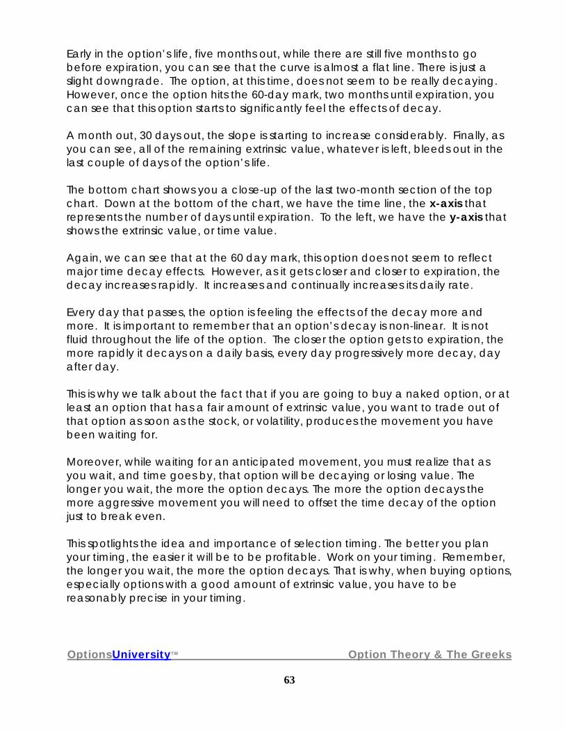
OptionsUniversityTM Option Theory & The Greeks
63
Early in the option’s life, five months out, while there are still five months to go before expiration, you can see that the curve is almost a flat line. There is just a slight downgrade. The option, at this time, does not seem to be really decaying. However, once the option hits the 60-day mark, two months until expiration, you can see that this option starts to significantly feel the effects of decay. A month out, 30 days out, the slope is starting to increase considerably. Finally, as you can see, all of the remaining extrinsic value, whatever is left, bleeds out in the last couple of days of the option’s life. The bottom chart shows you a close-up of the last two-month section of the top chart. Down at the bottom of the chart, we have the time line, the x-axis that represents the number of days until expiration. To the left, we have the y-axis that shows the extrinsic value, or time value. Again, we can see that at the 60 day mark, this option does not seem to reflect major time decay effects. However, as it gets closer and closer to expiration, the decay increases rapidly. It increases and continually increases its daily rate. Every day that passes, the option is feeling the effects of the decay more and more. It is important to remember that an option’s decay is non-linear. It is not fluid throughout the life of the option. The closer the option gets to expiration, the more rapidly it decays on a daily basis, every day progressively more decay, day after day. This is why we talk about the fact that if you are going to buy a naked option, or at least an option that has a fair amount of extrinsic value, you want to trade out of that option as soon as the stock, or volatility, produces the movement you have been waiting for. Moreover, while waiting for an anticipated movement, you must realize that as you wait, and time goes by, that option will be decaying or losing value. The longer you wait, the more the option decays. The more the option decays the more aggressive movement you will need to offset the time decay of the option just to break even. This spotlights the idea and importance of selection timing. The better you plan your timing, the easier it will be to be profitable. Work on your timing. Remember, the longer you wait, the more the option decays. That is why, when buying options, especially options with a good amount of extrinsic value, you have to be reasonably precise in your timing.

OptionsUniversityTM Option Theory & The Greeks
64
We will talk more about timing later when we talk about the purchase of a naked call or a naked put. What you need to know is that options decay and they decay at a progressively higher rate every day. You can see that on the decay chart above. Theta has affects on other components besides the overall dollar value of an option. For instance, time decay, or theta, affects delta. We have previously discussed delta and time’s affect on delta. So, we know that as time goes by, the delta of an option is going to change. If nothing were to happen at all, all things being equal, the delta of an option is going to change day to day as time passes. Theta and Delta Let’s take a look at the effect of theta on delta in “at-the-money” options, ‘in-the-money” options, and “out-of-the-money” options. Theta will affect the delta of each of these types of options, but will do so differently. We don’t really need to worry about whether the option is a put or call. Theta’s affects will be the same in both calls and puts. First, let’s take a look at an “in-the-money” option. Imagine we have an option that is $5.00 or so in the money and is 75 deltas with 30 days left to expiration. Now remember what that 75 deltas means. One of the definitions of delta, as you recall, is percentage chance. So, what we are saying here is that this option with a 75 delta has a 75 percent chance of finishing in the money at expiration. What can affect that expectation? Well, the stock could move. Volatility could increase or decrease. There are several things that can affect that 75 delta (that 75% chance of finishing in the money). Time decay, or theta, is one of them. Remember, the longer time an option has before expiration, the bigger chance there is for a major movement. So, this 75 delta option with 30 days left, with a 75 percent chance of finishing in the money, is going to have a higher percentage chance of finishing in the money after 15 of those days have gone by without anything happening. At that point this 75 delta option will have even more of a chance of finishing in the money because there is less time for something to happen to knock it out-of-the-money. Therefore, it will now trade with a higher delta, possibly, as high as 90. Why does the delta increase? The deltas of in-the-money options increase with the passage of time because as time goes by there remains a smaller amount of time for stock (or volatility) movement to change this in-the-money option into an
OptionsUniversityTM Option Theory & The Greeks
65
out-of-the-money option. At the 30 day mark, this option might only be 75 deltas. However, with 15 days left, the option might be 90 deltas. With only 15 days left, there is a much larger percentage chance that the option will finish in-the-money. There is much less time for it to not finish in-the-money. With two days left this 90 delta option might actually be 98 or 99 deltas, maybe even 100 deltas. Theta has influence over delta’s definition of percentage chance. Percentage chance in the option’s world is predicated by the amount of time left until the end of an option’s life. As long as the option exists, there is at least some kind of chance for something to happen. Remember what Yogi Berra said, “it ain’t over ‘til it’s over.” The same can be said of options. However, once it is over, at expiration, all in-the-money options will be 100 deltas and convert to stock. Theta affects the natural progression of delta’s movement over time. Theta, or time decay, affects the delta of in-the-money options by increasing their deltas as time passes with all other things being equal. Again, it is important to remember that the deltas of in-the-money options (both calls and puts) increase with the passage of time. In-the-money call options obtain higher positive deltas (get longer) while in-the-money put options obtain higher negative deltas (get shorter) as theta effects the option. Out-of-the-money options work the opposite way. Let’s take a look at an option that has 30 days to expiration, is $3.00 out of the money and has maybe a 30 delta. Fifteen days go by, and neither the stock nor volatility has moved. The option is still $3.00 out-of-the-money. But, half of that option’s life has gone by without any type of movement that could change the option’s price. That option will no longer be a 30 delta. Why? Because its percentage chance of finishing in-the-money has decreased further due to the fact that time has passed with nothing to stimulate an increase in the option’s price. Thus, its percentage chance of making that movement, with even less time to do it, is lowered. With only 15 days left, this option may then only be a 20 delta option. Theta, or the passage of time, decreases the deltas of out-of-the-money options. The less time the option has to move, the lower its chance of making the move. For an out-of-the-money option that means its delta has to decrease. So, out-of-the-money call deltas will decrease or become less positive (less long), while out-of-the-money put deltas will decrease or become less negative (less short) as theta effects the option.

OptionsUniversityTM Option Theory & The Greeks
66
Finally, let’s talk about at-the-money options. An “at-the-money” option is a little different than the other two. An at-the-money option, whose delta is around 50, is not going to be affected by the passage of time. Its price may be affected by theta in terms of price erosion, however, the option’s delta will not be. That is because that option is still on the fence between being in-the-money and out-of-the-money. In that sense, nothing has changed. If the stock was trading directly at the option’s strike price today, had been trading so 10 days ago, and will still be trading at the strike tomorrow, then the option still has a 50-50 chance of being either in-the-money or out-of-the-money at expiration. One cent one way or one cent the other is going to make the difference whether that option is in the money or out of the money and that does not change with the passage of time. In other words, this option’s status is going to be a coin toss that will come down to the last second. If we are looking at the 50 strike and the stock is trading at 50 right on the nose, a movement either up or down one cent is going to determine whether this option finishes “in” or “out” of the money. And that can happen on the very last stock tick on expiration Friday. Expiration Friday at 3:59 and that stock might be trading at $50 exactly. If the last tick at 4 o’clock is $50.01 the option is in-the-money and 100 deltas. If the last tick is $49.99, the option is worthless and out-of-the-money with zero deltas. All of this can happen in a split second, and more precisely, at the last moment before the last, closing stock price on expiration Friday. The days leading up to expiration are not as important for an at-the-money option as is the closing stock price at expiration. So, time is not really going to play a factor on that at-the-money option’s delta. Stock movement, not time, will be the deciding factor on delta. Theta is not going to have the same affect on at-the-money options as it will on an in-the-money or an out-of-the-money option. Theta is going to have very little effect on at-the-money options.

OptionsUniversityTM Option Theory & The Greeks
67
So let’s review Theta’s (time decay’s) effect on delta—which I feel is very important.
(I) When we talk about the in-the-money options, whether they are puts or calls, the passage of time increases the deltas of the in-the-money options. The reason for that is that with less time for the option to fall out of the money, obviously the percentage chance of the option staying in-the-money has to increase. That means the delta will have to increase.
(II) The passage of time, or theta, decreases the deltas of out-of-the-money
options, whether they are puts or calls. Why? Because with less time for the option to move from out-of-the-money to in-the-money, the percentage chance of that option doing it is decreased, thus a lower delta.
(III) As far as the at-the-money options, whether they are puts or calls, theta
has very little effect on those deltas. They are going to stay around 50. Why? Because the stock would need to make a very tiny or small movement to make that option become “in” or “out” of the money. It doesn’t have to move $5 or $6. It might only have to move a penny. And that type of movement can happen in one tick and it can happen at exactly 4:00 p.m. on expiration day. So time doesn’t play a big role in the delta of an at-the-money option.
Theta and Gamma Theta’s effect on Gamma is not a black-and-white issue. We can’t just say that the passage of time increases gamma positions. Nor can we say that the passage of time decreases gamma positions. Unfortunately, we can not make a simple blanket statement. We described above how theta affected the deltas of in-the-money, at-the- money and out-of-the-money options differently; theta is also going to effect gamma positions differently based upon where the gamma is located. Theta has a different gamma affect on different strikes. Its affect will be determined by where (the strike) the gamma is located. Theta affects the gamma of in-the-money options and out-of-the-money options differently than it affects at-the-money options. We saw this in theta’s affect on the deltas of options. B ecause gamma is a derivative of delta, the first derivative of delta to be precise, it marks the change in the delta. Therefore, it stands to reason that theta is going to have an effect on gamma also.
OptionsUniversityTM Option Theory & The Greeks
68
When we look at a long gamma position, we first have to check where the long gamma is located. If our long gamma position is located in an in-the-money or out-of-the-money option, the passage of time will work to decrease the size of the gamma position. Let me say that again. If our long gamma is located or positioned in an in-the-money or out-of-the-money option, all things staying equal, the passage of time will decrease that long gamma position. We know that the further the option is either “in” or “out” of the money, the quicker those deltas move to 100 or zero, and they move even quicker with the passage of time. At that moment when those deltas are either 100 or zero, they are probably not going to move much, if at all, other things being equal. And because those deltas don’t move much, the gamma has to be very small. The more they don’t move and the closer it gets to expiration, then obviously, the smaller and smaller those gammas get because the deltas are not moving and there is increasingly less time for them to move. So when talking about a long gamma position, if that long gamma is located in an in-the-money or out-of-the-money option, with all other things equal, the passage of time is going to decrease the size of that gamma position. However, if that long gamma position is located in an “at-the-money” option, whether it is a call or a put, the passage of time is going to increase that gamma position. The gamma will get larger. We hinted at this when we talked about gamma. Remember when we were talking about the 50 strike and the stock trading at exactly $50.00. We said that as you get closer to that final closing stock price on expiration day, if the stock is trading directly at the strike price - $50.00 – the smallest possible dollar increment move in that stock can and will create the largest delta movement possible. If this stock closed at $50.00 on the nose, the delta of that option will be zero. However, if the stock closed at $50.01, the delta of that option will be 100 for calls. For puts it is the opposite. If the stock closed at $49.99, then the puts would be 100 negative deltas. The important point here is that a one-penny stock move at the close on expiration will create a 100- point movement in delta. Delta can go from zero to 100 with a one-penny movement at the last closing price on expiration Friday. Keeping that in mind, remember what gamma measures. Gamma measures how much delta changes. At expiration, at that single moment in time, your delta can go from absolute maximum to absolute minimum, or absolute minimum to absolute maximum with one penny.

OptionsUniversityTM Option Theory & The Greeks
69
A one cent movement and an option can go from zero to 100 deltas or 100 to zero deltas. How big do you think gamma is at that moment? Gamma has to be gigantic at that moment. So if you are long an at-the-money call or put going into expiration, when gamma is the absolute biggest ever, you will see your long gamma position grow exponentially. The absolute largest that gamma can ever be occurs at 4 o’clock on the close of expiration day in an at-the-money option, whether call or put. That is the biggest that gamma will ever be, because that is where delta changes the most with the smallest possible movement in the stock. If your gamma position is located in an at-the-money option, it will continue to grow bigger and bigger as we move into the final tick of that stock on expiration Friday. So how does theta affect a long gamma position that is located at-the-money? It increases it, right into the closing bell on expiration Friday. How does theta affect short gamma positions? Much in the same way as it affects long gamma. Again, it all depends on where your short gamma is located. If your short gamma is located in an in-the-money option or an out-of-the-money option, theta will work to decrease your short gamma position. A short gamma position decreases as time goes by if the gamma is located in “in” or “out” of the money options. Just like long gamma positions, your short gamma positions located in “in” or “out” of-the-money options will decrease, all things being equal, as time goes by. And the reasoning is the same as it was for why it would decrease in long gamma positions for the in-the-money and out-of-the-money options. There is just less chance that those options are going to change their present “in” or “out” of the money status. Therefore, their deltas will approach either 100 or zero and with the continued passage of time, those deltas will move less and less thereby creating smaller and smaller gammas. As for a rule of thumb, we can say that as time goes by, theta decreases the size of gamma in “in” and “out” of-the-money options. What about the at-the-money option? The same theory that applies to long gamma positions also applies to short gamma positions. If your short gamma position is located at-the-money, then that short gamma position will increase in size, all the way into the final tick of the stock on expiration Friday.
OptionsUniversityTM Option Theory & The Greeks
70
That means your short gamma position, as time goes by, all things being equal, is going to increase in size (get shorter), up until the final closing stock tick on Friday of expiration, and for the same exact reasons that it would in a long gamma position. Remember, gamma measures how much delta changes. At expiration, your delta can go from absolute maximum to absolute minimum, or absolute minimum to absolute maximum with a stock movement as little as one penny. A one cent stock movement and an option can go from zero to 100 deltas or 100 to zero deltas. How big do you think that gamma is at that moment? Gamma has to be gigantic at that moment. So if you are short gamma in an at-the-money put or call going into the final moments before expiration, you will see your short gamma position grow exponentially. That is the biggest that gamma will ever be, because that is where delta changes the most with the smallest possible movement in the stock. If your gamma position is located in an at-the-money option, it will continue to grow bigger and bigger as time moves into the final tick of that stock on expiration Friday. As for a rule of thumb, it can be said that an at-the-money option’s gamma will grow (get larger) as time passes into expiration. So, let’s review and consolidate this concept. What is theta’s affect on gamma positions as a whole? It depends on where your gamma position is located. That is the key. How is theta going to affect your position? It depends on where your gamma position is located. If it is in an in-the-money or out-of-the-money option, it is going to decrease the size of whatever gamma position you have whether long or short. If you have a long gamma position, it is going to get shorter. If you have a short gamma position, it is going to get longer. Theta is going to decrease your gamma, moving it toward zero. If your gamma position is located in an at-the-money option, whether put or call, whether long or short, whatever gamma position you have, the passage of time, or theta, will increase that gamma position. It will make a long gamma position longer, and it will make a short gamma position shorter. It is as simple as that. Obviously, theta has a real close working relationship with gamma. That happens since the way you obtain theta is the same way you obtain gamma, by either buying or selling options. In a sense, gamma and theta are two peas in a pod. Where you have one, you have the other. We know that you obtain long gamma by buying options. We know that you obtain short gamma by selling options. Theta is obtained in the exact same manner. In fact, you can not have gamma without theta and you can not have theta without gamma.

OptionsUniversityTM Option Theory & The Greeks
71
Although they come together and are indeed inseparable, gamma and theta also have an inverse relationship. It is very simple. Think for a second. You obtain long gamma from purchasing options but, at the same time, that option purchase creates decay, a negative theta. Why? This is because your option purchase creates a positive gamma position while your premium purchase creates a time decaying scenario. On the other hand, when you sell an option you create a negative gamma position while your premium sale creates a positive collection scenario. Consider the relationship between gamma and theta. If you own an option, you’re going to be long gamma. And if you are long gamma, then you’re going to be paying for it. That means you are going to be short theta. If you are short an option, you are going to be short gamma. And if you are short gamma, you are going to be collecting from it. That means you are going to be long theta. Another little relationship between gamma and theta is this: where gamma is the highest, theta is the highest. Let me say that again. Where gamma is the highest, theta is the highest and vice-versa.
THETA CHART
.006.011.020.01880
.009.017.024.02875
.016.024.038.05570
.018.026.042.05965
.011.019 .033.04160
.007.010.013.01355
.005.006.007050
JanuaryOctoberJulyJuneStrike Price

OptionsUniversityTM Option Theory & The Greeks
72
That brings us to the theta chart. Looking at it you are going to see something that looks very familiar. A theta chart tells you the rate of the decay of each option. Now I said the theta chart is going to look very familiar. It does because of its pattern. Compare the theta chart to the gamma chart, and ask yourself where gamma is the absolute highest. We already know that gamma is going to be the absolute highest in the front month, at-the-money strike. Now, look on the theta chart and ask where theta is going to be the highest. Coincidently, it also is going to be highest in the front month at-the-money strike. Now, let us compare as we move away from the at-the-money strike, in either direction. We notice that gamma decreases as we move away from the at-the-money strike and so does theta. When we look at the theta chart, we see that the at-the-money strike is the 65 strike. If we move down to the 60 strike, theta decreases. If we move up to the 70 strike, theta decreases. And, as we move progressively out in either direction, the amount of theta continues to decrease, just like gamma. Well what about going out over time? We know that when you go out over time, gammas decrease. Let us compare this to theta. Look at the June 65 strike where the theta is almost $0.06. Now let us look at the July 65 strike. We notice that the theta value has decreased. The theta in the October 65 strike is lower than the July 65 strike and the January 65 strike is the lowest of the 65 strikes. This is showing the time decay curve, an obviously non-linear function. As you can see, the further we go out in time, the smaller the theta is. So, your theta chart and your gamma chart are going to look identical in their pattern. This is not a coincidence! Why? Because where gamma is the highest, theta is the highest and vice-versa. When we look at theta, theta is always highest, front month, at-the-money. In any given month, as you move away from the at-the-money strike, theta decreases. As you go out over time, across any single month, theta decreases. Now there is a little aberration that occurs here. Look at a deep in-the-money strike, and a deep out-of-the-money strike, the 50 strike and the 80 strike, for instance. You can see that in your July 80 strike, you actually have a little higher theta than in your June 80 strike. This violates our rule of thumb. The reason is the June 80 strike is starting to become so far out-of-the-money that it is losing all of its sensitivities. It is becoming worthless and losing its “status” as an option. Same thing when you look at your June 50 strike. You can see that the June 50 strike has lost all of its sensitivity.

OptionsUniversityTM Option Theory & The Greeks
73
There is a decrease in theta because the June 50 strike is now stock. It is so deep in-the-money that it is like stock. It is 100 deltas. There is no more option related sensitivity in the June 50 strike because it is now considered to be stock. As you know, stock has no theta. This is why you will sometimes see an increase in theta from a front month option (such as the June 50) to an outer month option (such as the July 50). This will only occur in deep in-the-money and far out-of-the-money options near expiration. So, when you see that, do understand it. But, even in this situation, the theta chart looks exactly like the pattern of the gamma chart! In conclusion, here is are some highlights of the important concepts about Theta.
1. Theta measures an option’s rate of decay over time.
2. Theta affects an option’s extrinsic value.
3. Theta’s affect on options is nonlinear.
4. Theta affects not only an option’s price but also its delta and gamma.
5. Theta affects the gamma and delta of the 3 option categories differently.
6. Theta (time decay) is a 7 day, 24 hour a week happening.
7. Theta has a special relationship with gamma that is observable on graphs.
8. Theta gives a good idea of what an option will do as time passes. That is what Theta is about!
OptionsUniversityTM Option Theory & The Greeks
74
Second Tier Greeks
We have discussed all of the front line Greeks - those major outputs of the pricing model, more commonly referred to as the first-tier Greeks. There are, however, other levels of Greeks. The one we are concerned with in this discussion is called the “second-tier Greeks.” These Greeks do not directly measure a stock or an option. They measure, using a number, the change in a first-tier Greek caused by changes in certain variables. They quantify the front line Greeks’ sensitivities to changes to outside factors such as time and volatility. There are many second-tier Greeks, but I picked out the five that I believe are important for you to know and that are going to be important for your success as an investor/trader… The particular second tier Greeks discussed below are important because they quantify (using a specific number) a special relationship between two of the major Greeks – a relationship that may effect your positions or portfolio. The effect of one part of the relationship on the other is expressed in numbers. In the interest of clarity, let’s identify the relationships: V-Delta (V-Del) measures a change in volatility’s effect on delta. T-Delta (T-Del) measures the passage of time’s (theta’s) effect on delta V-Gamma measures a change of volatility’s effect on gamma T-Gamma measures the passage of time’s effect on gamma V-Theta measures a change in volatility’s effect on theta The first important relationship is V-Delta. V-Delta measures the change in volatility’s influence on delta. We have discussed this before. We have also discussed what volatility changes did to the deltas of individual options. V-Delta tells you what the change in volatility is going to do to the overall delta of your position, or to the overall delta of your entire portfolio. It is important to understand what V-Delta measures and how it measures. V-Delta connects volatility and delta. It creates an actual number for us to determine the effects of that relationship; plus 400, minus 1,500, plus 60, minus 97. A positive V-Delta or V-Del tells you that for each tick volatility moves, your delta position will either increase or decrease by a set amount of deltas. For instance, suppose you have a positive 500 V-Del and volatility is trading at 35.

OptionsUniversityTM Option Theory & The Greeks
75
Your new overall delta position would increase by 500 deltas if volatility went to 36. Meanwhile, if volatility were to go down a tick, down to 34, then your position would decrease 500 deltas. If you had a negative V-Del and the volatility went up, your delta position would decrease by the amount of V-Del components you had. If you had a negative V-Dell and volatility went down, then your delta position would decrease by however many V-Dells you were short. When does this become important? This becomes important when a stock has a major volatility move. I am not talking a tick or two. I’m talking a minimum of 10 to15 ticks, a 20, 30, 40 percent increase. You have to know what your real delta is at that new volatility level. V-Del tells you that. T-Del, or T-Delta, measures the theta to delta relationship. It tells you how your delta position will change (by what amount) with the passage of time. This second tier Greek is not evaluating a movement in volatility; it is evaluating the effects of the movement of time. How does the movement of time, all things being equal, affect your delta position? If you are positive T-Del, it means your delta position gets longer as the days go by. If you are short T-Del then your position —your delta position—gets shorter as the days go by. You might see the value of V-Del but question the value of T-Del. How is it important? T-Del helps when you are going to be away from your position for a time. We touched on this when we discussed Theta. Time decay happens even when the market is not open! When you leave for a long weekend, a vacation etc. you know where your delta position stands at that time, however, it will not be the same when you get back. T-Del tells you what you can expect when you return. Your delta position is going to be different, and potentially vastly different, when you get back. Even if the stock hasn’t moved, even if the stock and volatility have not moved, the passage of time, those days gone by, are going to affect your delta position. T-Del tells you by exactly how much. If your T-Del is a positive 100 then that means that one day from now, with all things being equal, your new delta position is going to be longer by 100 more deltas. Two days go by, 200 long deltas, three days, 300 longer deltas. That is what T-Del tells you; by how much per day your delta position is going to increase or decrease with all things being equal, and with the only changing variable the passage of time.

OptionsUniversityTM Option Theory & The Greeks
76
Although V-Gamma is not as important as V-Del, volatility levels definitely have an affect on your gamma position. You need to understand V-Gamma especially if you are gamma trading. You need to know not only how the movement or changes in implied volatility affect your gamma position, but you also need to know by how much. As stated before, for those of you who are going to be interested in gamma trading, you need to know what your gamma is at all times under every condition in order to trade it effectively. That gamma level will be affected by changes in implied volatility. As a rule of thumb, increases in volatility decrease the size of your gamma position. Whether you are long gamma or short gamma does not matter. An increase in implied volatility will decrease the size of your gamma position. If you are long gamma and implied volatility increases, you will get shorter gamma. If you are short gamma and implied volatility increases, you will get longer gamma. V-Gamma tells you by what amount gamma is going to change per one tick change in implied volatility. It’s as simple as that. Continuing with our rule of thumb, a decrease in implied volatility will increase the size of your gamma position. If you are long gamma and implied volatility decreases, you will get longer gamma. If you are short gamma and implied volatility decreases, you will get shorter gamma. T-Gamma works in a similar way as V-Gamma, except that the T-Gamma relationship is not evaluating changes in implied volatility. T-Gamma is evaluating the affect of the passage of time, theta’s affect on gamma. T-Gamma, like T-Delta, tells you what to expect when you are away from your position. You leave knowing the gamma of your position. You return and your gamma position is now different. Remember, we just said that time goes by, whether the market is open or not and the passage of time will have an affect on your gamma position. How? The more time that goes by, the larger your gamma position gets. The passage of time increases the size of your gamma position. So, if you are long 500 gammas on Thursday afternoon, you might be long 600 gammas when you check them on Monday morning. If you are short 200 gammas the day before Fourth of July weekend, you may be short 300 gammas when you come back from the holiday weekend. Beware, there is a slight monkey wrench thrown into T-Gamma. Hopefully, some of you have remembered what we talked about in terms of gamma and theta’s affect on gamma.

OptionsUniversityTM Option Theory & The Greeks
77
Theta’s affect really depends on where your gamma is located. Theta’s affect is different depending on whether gamma is located in “in the money” options, “out of the money” options or in at-the-money options. As we approach expiration, the “in the money” and the “out of the money” options start losing their option-ness. As these options near expiration they either become worthless because they are way out of the money with little or no extrinsic value, or they become stock because they are so far in the money. And we know that something with no extrinsic value has no delta gamma, vega, or theta. And we know that something that is stock has no gamma, vega or theta. The lesson here is that as the in-the-money and out-of-the-money options get close to expiration, they will lose gamma. This is contrary to our rule of thumb. There is a point in time when these options will no longer gain gamma as time progresses but will start to lose gamma. That point in time is near the very end of the option’s life. The “at-the-money” option, however, will continue to gain gammas up until the final minute of its life provided the stock is still trading at the strike price. Therefore, you have to be cautious with T-Gamma. Not gigantically cautious, but you have to be aware. Being aware of the specific location of gamma is also true for V-Gamma. Not nearly as much as with T-Gamma, but you have to know where your gamma position is located and how that option is going to behave as it gets closer to expiration. Remember earlier when we examined the appearance of gamma on its chart you saw gammas in the way out-of-the money and the way in-the-money options decrease a bit as they approached expiration. However, the “at-the-money” gamma got much bigger, in fact it exploded. That is the glitch that you must be aware of with gamma. You absolutely must know where your gamma is located. Is it located in an “at-the-money” option, or is it located further away from “at the money.” Is it “deep in the money”, or “deep out of the money”? Keep that in mind. But, the purpose of T-Gamma is to tell you how the passage of time is going to affect your gamma position no matter where it is located. The final second-tier Greek that is of special interest to us is V-Theta, which measures the affect of a change in volatility on theta. Now this one is easy. Recall what we know about volatility’s affect on option prices. We know that if volatility increases, then option prices, all option prices, both puts and calls, increase. On the other hand, when volatility decreases, the value of all options (both puts and calls) decreases. So, when implied volatility goes up, prices go up; when implied volatility goes down, prices go down.

OptionsUniversityTM Option Theory & The Greeks
78
How does that affect theta, your rate of decay? Volatility affects the prices of options by either increasing the amount of extrinsic value in the option (when volatility increases) or by decreasing the amount of extrinsic value in the option (when volatility decreases). The more extrinsic value present in that option, the more it has to decay. An option that has $1.25 of extrinsic value with 30 days left to expiration has to decay $1.25 in the remaining 30 days. However, that same option priced at $1.50 (after an increase in volatility), now has $1.50 worth of decay over the 30 days remaining to expiration. That demonstrates that the more volatility goes up, the more theta you have in an option. That more expensive option has more to decay. V-Theta, or the volatility to theta relationship, basically tells you, with a number, how much your decay is going to change with a movement in implied volatility. Now are these tools critical? In my mind, yes they are. You need to be properly instructed on how different changes in the different influencing factors of option pricing will affect your position, your investment. You need to know your risks! These second tier Greeks help you understand what is going to happen, or what can happen to your position before it happens, not after. No one should enter a trade without knowing and understanding what their risks are!!! The beauty of the second tier Greeks is they tell you what can happen to your position in an “if” scenario. If volatility goes up, this will happen to your delta. If theta goes down, this is what will happen to your delta. If volatility increases, this is the affect, or could be the affect on your gamma position. The passage of time will cause this amount of change in your gamma position. Volatility affects your theta by this amount. All of these scenarios can affect your position thereby affecting your profit and loss. Knowledge of the second-tier Greeks prepares you to handle and adjust your position to account for what can happen. And if you can stay prepared, you are going to do much better in trading. That is the particular significance and importance of the second-tier Greeks. They give a concrete expression, a number, to the changes brought on by implied volatility and by the passage of time.