Option Contracts in Supply Chains∗

Apostolos Burnetas� Peter Ritchken�

March 14, 2002

∗The authors thank Ranga Narayanan, Vishy Cvsa, and the participants of a seminar at the Department ofManagement of the University of Texas at Austin for helpful comments.

�Department of Operations, Weatherhead School of Management, Case Western Reserve University, 10900Euclid Ave., Cleveland, Ohio, 44106, Tel: 216-3684778, Fax: 216-368-4776, E-mail: atb4@po.cwru.edu

�Department of Banking and Finance,Weatherhead School of Management, Case Western Reserve Univer-sity, 10900 Euclid Ave., Cleveland, OH 44106-7235, Phone: (216) 368�3849, Fax: (216) 368�4776, E-mail:

phr@po.cwru.edu

Abstract

This article investigates the pricing of options when the demand curve is downward sloping.

Our speciÞc application arises in a supply chain setting, where a manufacturer offers the retailer

the right to reorder items at a Þxed price and/or the right to return unsold goods for a prede-

termined salvage value. We show that the introduction of option contracts causes the wholesale

price to increase and the volatility of the retail price to decrease. Conditions are derived under

which the manufacturer is always better off by introducing options. In general, options are not

zero sum games. In some cases the retailer also beneÞts while in other cases the retailer is

worse off. If the uncertainty in the demand curve is sufficiently high, the introduction of option

contracts alters the equilibrium prices in a way that hurts the retailer. Finally, we demonstrate

that if either the manufacturer or the retailer wants to hedge the risk, contracts that pay out

according to the square of the price of a traded security are required.

Many studies have been performed in industries such as apparel, sporting goods and toys,

where there are long lead times, short selling seasons and high demand uncertainties. For these

problems one avenue of research is concerned with the design of contracting relationships that

provide retailers with ßexibility in responding to unanticipated demand and prices over the

sales season. This paper examines such contracting arrangements in a supply chain setting

consisting of an upstream party (which we refer to as the manufacturer) whose only access to

the product market is via a single downstream party (which we refer to as the retailer). To

manage the risk of inventories associated with uncertain demand, it is fairly common for the

manufacturer to provide the retailer with an array of products, including reordering contracts,

or call options, that allow the retailer to purchase additional goods at a predetermined time for

a Þxed price, and return contracts, or put options, that allow the retailer to return unsold goods

at a predetermined salvage price. By purchasing inventory, together with a portfolio of these

supply chain call and put options, the retailer has more choices that allows a strategy to be

put into place to best meets its interests. The manufacturer�s goal is to design the terms of the

reordering and return option contracts and establish their prices, together with the wholesale

price, so as to induce the retailer to take optimal actions that best serve the manufacturer�s

interests.1

By introducing reorder and return option contracts, the manufacturer alters the retailer�s

sequence of decisions. This in turn has a feedback effect in that the equilibrium wholesale

and retail prices are affected. In this paper we are particularly interested in how these prices

adjust after the introduction of supply chain options. We are also interested in establishing

the pricing mechanism that the manufacturer uses for the supply chain options. Indeed, our

problem environment is set up so that we can closely examine the pricing of option contracts

in a downward sloping demand curve environment. Moreover, since we assume that there are

sufficient Þnancial products that span all uncertainty, we are able to unambiguously value the

beneÞt of the supply chain options without explicitly incorporating risk aversion factors.

The usual approach in pricing real options follows the Black-Scholes (1973) andMerton (1974)

paradigm, in which contracts are replicated by dynamic self Þnancing trading schemes in the

underlying asset and in riskless bonds. In this approach, derivative contracts are redundant and

do not affect prices of assets in the marketplace. In order to investigate how derivative contracts

might impact prices, it is necessary to move away from the typical partial equilibrium arbitrage

free paradigm and to allow for the possibility that these claims have feedback effects that may

alter equilibrium prices of the underlying assets.

In the Þnancial options literature, there is a large number of studies that have investi-

1The existence of multiple decision makers with different ownership interests results in departures from Þrst-

best solutions and creates strong incentives for parties to enter into contracts that enhance system-wide perfor-

mance and improve channel coordination.

1

gated how listed option contracts could alter the dynamics of asset prices. The popular view

that derivatives were beneÞcial because they expanded the investment opportunity set, allowing

traders to more precisely mold returns in accordance with their beliefs and preferences, lacked

rigor, because it ignored potentially harmful feedback effects. Theoretical models that explore

these feedback effects draw different conclusions. Detemple and Selden (1988) as well as Gross-

man (1988) identify different sets of conditions whereby the introduction of options leads to a

reduction in volatility of prices, whereas Stein (1989) identiÞes conditions that lead to increased

volatility. The empirical evidence, provides modest support for options to lead to reductions

in volatility.2 The empirical literature also concludes that the listing of call (put) options is

associated with positive (negative) excess abnormal returns on the underlying asset, while the

simultaneous listing of both has little effect.3 The results of our analysis in the real options

setting echo some of the results from this literature in the sense that we Þnd the introduction

of supply chain options is accompanied by price effects, both at the wholesale and at the retail

levels. In particular, we show that retail prices are less volatile then they would be if no options

were utilized. We also identify conditions under which retail prices may increase, or decrease.

Finally, with regard to wholesale prices, we show that they will either stay the same or increase.

In our framework, the beneÞt of the option program to the manufacturer is inßuenced by

the uncertainty in the demand curve and the cost of fulÞlling expedited orders that arise from

options being exercised late in the season. The manufacturer will only introduce options if

they increase proÞts. Expanding the investment opportunity set, however, may not necessarily

improve the condition of the retailer. Indeed, we show that when the demand curve is very

uncertain, then the retailer is worse off when options are introduced. This result may, at Þrst

glance, be a bit surprising, since one might surmise that when uncertainty is high, the retailer

will be more inclined to use option contracts. Of course, the manufacturer recognizes that this is

the case, and adjusts the wholesale and option prices accordingly. The option contracts are not

zero sum games between the manufacturer and the retailer, and, as we shall see, there are cases

where both parties beneÞt. The pricing of the supply chain options is of particular interest.

The reorder options are shown to be less valuable than otherwise identical cash settled contracts

based on the equilibrium retail price. This result is tied to the fact that in a downward sloping

curve environment, options that appear to be �in-the-money� at expiration, may rationally go

unexercised.

The equilibrium wholesale price can be affected by the introduction of reorder options.

However, once introduced, we show that the wholesale price will not readjust again if the man-

ufacturer chooses to introduces return options, provided the range of strike prices are curtailed.

2Examples of studies include Damodaran and Lim (1991) and the references in Damodaran and Subrah-

manyam (1992).3Surprisingly, Conrad (1989) Þnds that the abnormal returns are generated around the listing date, rather

than the earlier announcement date.

2

Finally, we show that the net present value of proÞts for the manufacturer and retailer can be

related to the value of a highly nonlinear derivative claim. In particular, their values are fully

determined by the price of an option that has payouts based on the square of the price of a

traded security. While Jarrow and van Deventer (1996) have used these contracts, often referred

to as power options, in pricing demand deposit accounts, this economic justiÞcation, in a real

option setting, is, as far as we know, new.

The paper proceeds as follows. In section 1 we review related literature from supply chain

management. In section 2 we list the basic assumptions and establish the decision and pricing

problems. We formulate the problem for the case where the manufacturer is considering the use

of reordering options. Later on we show how the solutions to this problem can be used to solve

for the returns option policies and their prices. In section 3 we establish the benchmark case,

where the manufacturer does not provide the retailer with any option contracts. This situation is

of some interest in its own right. SpeciÞcally, after purchasing inventory, the retailer retains the

option to withhold some product from the market. This retention option is shown to be valuable,

especially when there is large uncertainty in the demand curve. In section 4 we consider the case

when the retailer is allowed to purchase reorder options with inventory purchases. We closely

investigate how the equilibrium wholesale price and retail prices are affected by the introduction

of such contracts. In section 5 we isolate conditions under which both parties beneÞt from the

option program. We also identify cases where the option program beneÞts the manufacturer,

but not the retailer. The value of the option program is also related to the value of a derivative

instrument that has payouts linked to the square of the price of a traded security. Section 6

examines the consequences of a returns policy and shows that the equilibrium prices can be

obtained from the solution to the earlier gaming problems. Section 7 extends the results to

cases where the uncertainty in the linear demand curve follows a more general distribution than

that prescribed earlier. We illustrate that our above results hold true when uncertainty in the

linear demand curve follows a continuous distribution.

1 Literature Review

Building large inventories can be expensive if large demands are not realized. Of course, not

building inventory can lead to shortages with large opportunity costs. These trade offs need

to be carefully assessed. One way for the retailer to manage this risk is to transfer it to the

manufacturer who may be better equipped to absorb it. Contracts are designed not only to

meet the risk aversion needs of the parties in the supply chain, but also to help coordinate the

channel. Examples of contracting relationships include Eppen and Iyer (1997), who consider

back up agreements, Serel, Dada and Moskowitz (2001), who consider capacity guarantees,

and Brown and Lee (1997), who consider pay-to-delay capacity reservation contracts. Barnes-

3

Schuster, Bassok and Anupindi (2000), show that all of these contracts can be viewed as special

cases of option contracts that permit expedited orders. For excellent reviews of this literature

see Anupindi and Bassok (1999), Lariviere (1999) and Tsay Nahmias and Aggrawal (1999).

Within this literature, an important consideration is channel coordination. Oftentimes this

can be accomplished through non linear pricing as in Iyer and Bergen (1997). In other cases,

coordinating the supply chain is accomplished by modifying the contract between wholesalers

and retailers. For example, Barnes-Schuster, Bassok, and Anupindi (2000), show that channel

coordination could be achieved by modifying the nature of the strike price in their contracting

arrangements. Other examples of contracting mechanisms that induce channel coordination

include Pasternak (1985), who considers product returns, and Taylor (2001), who considers

combination of returns and retailer price protection. In these studies the typical methodology

employed builds off the classical newsvendor model where inventory levels are established before

demand is realized.

Our study is related to the above papers in that we consider contracting arrangements in a

supply chain in a newsvendor environment. Our approach, however differs in that we do not take

the retail price and the demand distribution as given; rather, we assume demand distributions are

inßuenced by pricing decisions. In particular, we assume the retailer is faced with an uncertain

downward sloping demand curve, and hence has to establish a retail price conditional on previous

inventory decisions. In this regard our analysis relates to an extended single agent newsvendor

problem discussed by Petruzzi and Dada (1999), who permit stocking policies and prices to

be determined simultaneously. It also relates to Ritchken and Tapiero (1986) who investigate

option contracts for purchasing decisions, in which price and quantity uncertainty are correlated.

Both these studies deal with single agents, whereas our analysis deals with two agents in the

presence of an uncertain linear downward sloping demand curve.

Several studies have investigated contingent claim pricing in the presence of a downward

sloping demand curve. Triantis and Hodder (1990) examine the pricing of complex options that

arise in a ßexible production system which allows the Þrm to switch its output mix over time, in

the presence of demand curves which are stochastic and downward sloping. Pindyck (1989) and

He and Pindyck (1989) also incorporate downward sloping demand curves to examine capacity

choice decisions in a real options framework. Our study differs from these in that we have a

speciÞc supply chain in which the optimal contracts can be designed and priced through the

appropriate use of principal-agent theory.

2 The Basic Model

We consider a simple supply chain consisting of a single manufacturer who produces a product

and sells it at a wholesale price to a retailer. At date 0, the future date 1 demand curve

4

is uncertain. Without any risk management contracts, the retailer is faced with bearing this

risk. The manufacturer assists in risk sharing by allowing the retailer to supplement inventory

decisions with option purchases. Each option contract provides the retailer with the right to

purchase an additional unit at date 1, after uncertainty is revealed, for a predetermined price of

X dollars.

Let I and U be the number of goods and options purchased at date 0 by the retailer. The

price of each good is S0 and the price of each option is C0. The retailer�s problem is to determine

the optimal mix of inventory and options, given their prices. The manufacturer�s problem is

to establish the optimal prices of both the product and options that induces the retailer to

take rational decisions that further the interests of the manufacturer. The manufacturer is

particularly keen to access the value to the Þrm of issuing option contracts and to assess the

role of the strike price of the contract.

We assume the demand in period 1 is linear. Denoting period one prices by S1, the inverse

demand curve is:

S1 = α− δQ (1)

where Q is the total amount of inventory released into the market. Here α is stochastic, and if

δ > 0, α/δ can be viewed as the maximum potential size of the market.

At date 1 the uncertainty in the market size factor, α, is resolved, and the retailer responds

by establishing how many units of inventory to release into the market and how many options

to exercise. Let 0 ≤ q ≤ I be the number of units of inventory released and let 0 ≤ v ≤ U be

the number of options exercised. The total number of items released into the market place is

Q = q + v. We assume that any excess inventory that is held back has no salvage value. 4 Let

R1 be the net cash ßow that the retailer makes in period 1. Then

R1(q, v|I, U,α = a) = (q + v)(a− δ(q + v))− vX (2)

In period 1, the retailer chooses q and v to maximize equation (2) subject to the inventory and

option constraints. If the exercise price X is too high, then the retailer, who has exclusive rights

to the market, has incentives to renegotiate the price. To ensure that the option contract is

credible, the manufacturer must therefore set the exercise price no higher than the marginal

cost of expedited production in period 1. 5

Now, consider the retailer�s decision at date 0. Let R0 be the net present value associated

with purchasing I units of inventory and U options at date 0 and optimally managing the project

in period 1. Then

R0(I, U) = −IS0 − UC0 + E[R1D1] (3)4This is consistent with a downward sloping demand curve.5This assumes that the manufacturer builds to order and is faced with a linear cost structure. Note that if the

exercise price is set too low, then the retailer is exposed to the risk of the manufacturer defaulting.

5

where D1 is the state dependent stochastic discount rate, commonly referred to as the pricing

kernel.

We assume uncertainty in the demand curve is represented by a Bernoulli process. In par-

ticular:

α =

(aH with probability p

aL with probability 1− p (4)

We also assume that there exists a traded security that pays out aH dollars in the high (H)

state, and aL dollars in the low (L) state. The price of this security at date 0 is A0. In addition,

a riskless bond exists that pays out $1 in period 1. Its current price is B0 < 1. The existence

of traded securities that spans the uncertainty in the demand curve allows the pricing kernel to

be uniquely determined.6 This assumption allows us to perform the valuations without regard

to the speciÞc risk preferences of the retailer and manufacturer. In addition, the valuation can

proceed, even if there is not consensus on the value of p.

Let eH (eL) be the Arrow Debreu state prices corresponding to a $1.0 payout only in the

high (low) state and $0 payout otherwise. Clearly:

A0 = aHeH + aLeL

B0 = eH + eL.

Given the state prices we have:

R0(I, U) = −IS0 − UC0 + eHR1(q∗H , v∗H |I, U, aH) + eLAR1(q∗L, v∗L|I, U, aL), (5)

where R1(q∗H , v

∗H |I, U, aH) and R1(q∗L, v∗L|I, u, aL) are the maximum values of R1 in equation (2)

with α = aH and α = aL respectively.

The retailer�s time 0 optimization problem is given by

MaxI≥0,U≥0R0(I, U) (6)

The objective of the manufacturer is to maximize value by appropriately determining the whole-

sale price, S0, and the charge for each option, C0. Let M0 be the net present value associated

with this speciÞc project. Then.

M0 = IS0 + UC0 + eH [Xv∗H ] + eL[Xv

∗L]−K0(I)− eHKH(v∗H)− eLKL(v∗L). (7)

In this equation, K0(I) represents the total cost of making up I units for delivery at date 0,

and KH(v∗H) (KL(v

∗L)) represents the cost of expediting an additional v

∗H ( v

∗L) units on date 1 in

the high (low) state. For simplicity, we shall assume that all costs are linear, i.e., K0(q) = K0q,

6For an in depth discussion on this point see Duffie (1996).

6

KH(q) = KHq and KL(q) = KLq, where K0,KL, KH are known constant marginal production

costs. To ensure that the manufacturer prefers committed orders to expedited orders, we require

KjB0 > K0 for j = L,H . Further, to ensure that the manufacturer does not Þnd it advantageous

to build inventories as a contingency we require K0 ≥ Kjej, for j = L,H . Finallly, we assumethat K0 < A0, since A0 represents the value at date 0 of a unit of product sold at the highest

possible retail price in date 1.

The manufacturer�s problem is to establish the wholesale price, S0, the reorder option price,

C0, and the appropriate strike, X , such that:

MaxS0,C0,XM0(S0, C0,X) (8)

given the fact that the retailer responds optimally for each action. This formulation is a standard

principal-agent problem, or Stackelberg game, with the manufacturer being the principal.

In what follows we often Þnd it helpful to represent the uncertainty in the demand curve in

terms of volatility. Let µA and σ2A represent the mean and variance of the intercept term of the

demand curve under the risk neutral measure.7 Then

µA =A0B0

σ2A =eHeLB20

(aH − aL)2,

and we have:

aH =A0B0

+√ρσA

aL =A0B0

− 1√ρσA

where ρ = eLeH.

3 Pricing with no Supply Chain Option Contracts

We begin by considering how the retailer will respond to a given price set by the manufacturer.

Lemma 1

If the manufacturer does not provide options, the optimal quantity of inventory the retailer

7Under this measure the expected growth rate of all traded securities equals the risk free rate. In this model

it is determined by the two risk-neutral probabilities qj = ej/B0, j = L,H.

7

orders at time 0 is given by:

I∗ =

aHeH−S02δeH

if 0 < S0 ≤ (aH − aL)eHA0−S02δB0

if (aH − aL)eH ≤ S0 ≤ A00 if S0 > A0.

Proof: See Appendix

Lemma 1 implies that the quantity ordered by the retailer decreases as the wholesale price

increases, Þrst at a low rate up to a critical point, and then at a faster rate. Given the response

function, the manufacturer can establish the optimal pricing policy. The results are summarized

below.

Proposition 1

(i) With no options, the manufacturer�s optimal pricing policy is:

S∗0 =(

A0+K02 if σA ≤ η(K0)

aHeH+K02 if σA > η(K0)

(9)

where

η(K0) =

√ρ

1+ ρ+√1+ ρ

∙(1+ ρ)

K0B0

+p1+ ρ

A0B0

¸ρ =

eLeH.

(ii) The retailer�s optimal ordering and selling response is

I∗ = A0−K04δB0

, q∗L = I∗, q∗H = I

∗ if σA ≤ η(K0)I∗ = eHaH−K0

4δeH, q∗L =

aL2δ , q∗H = I

∗ if σA > η(K0)

Proof: See Appendix

The proposition tells us that the manufacturer chooses a higher price if the variance is lower

than a threshold value, η2(K0), and a lower price otherwise. To gain insight on this result, Þrst

consider the case where there is no demand uncertainty, namely σA = 0. In this case, it is easy

to show that the equilibrium wholesale price is S0 =A0+K0

2 and the optimal order quantity

is I = A0−K04δB0

. If σA ≤ η(K0), this wholesale price and retailer response remains optimal.

SpeciÞcally, the retailer will ensure enough inventory is purchased so that in the low state the

optimal quantity is released, while in the high state there is only minor regret.

As the volatility expands, the consequences are no longer minor. Eventually, the retailer will

want to order more than is required for the lower state, but not enough to cover the optimal

amount in the high state. If the low state occurs, the retailer has to establish the amount to be

8

released into the market. By retaining some of the units, the retailer ensures a higher per unit

cost. However, since the units are costly, the retailer will take this into account when the he

makes the ordering decision in period 0, and will be less likely to order too much. The retailer�s

ability to control how much inventory is released into the market is called a retention option.

As the volatility of the demand curve expands, the value of this retention option also expands.

The ability of the retailer to control the number of items that are released for sale is valuable,

and is recognized by the manufacturer. Indeed, it can be shown that if the retailer was committed

to releasing all inventory that was ordered in period 0, then the manufacturer would set the

equilibrium price at A0+K02 regardless of the variance.

The manufacturer, recognizes the importance of the retailer�s retention option, and induces

the retailer to purchase more inventory, by offering a lower price when the variance is large

(σA > η(K0)). The retailer responds to the lower price by purchasing more units than necessary

for the lower state, but not quite enough for the high state. Since the gap between states is

sufficiently large, and since the per unit cost is low, the retailer is prepared to withhold some

inventory in the low state, rather than releasing it into the market.

For the low variance scenarios, the retailer has little incentive to build excess inventory,

beyond what is optimal for the lower state, since the additional revenues captured by having

such inventory available, if the high state occurs, does not offset the additional costs of purchasing

inventory at date 0, which may go unused. The manufacturer, of course, recognizes that the

retention option is not worth much, and hence charges a price, based on the premise that the

retailer will rationally commit to selling all inventory purchased.

The table below summarizes the wholesale and retail prices in periods 0 and 1 respectively,

together with the state dependent quantities that are released into the market place.

Variance Wholesale Order Amount Released Retail Price

Price Quantity

S0 I0 qL qH SL SH

σA ≤ η(K0)A0+K0

2A0−K0

4δB0A0−K0

4δB0

A0−K0

4δB0aL − A0−K0

4B0aH − A0−K0

4B0

σA > η(K0)aHeH+K0

2eHaH−K0

4δeHaL2δ

eHaH−K0

4δeHaL2

3aH4 + K0

4eH

9

4 Pricing with Supply Chain Option Contracts

We now reconsider the above problem, but this time we also assume that the manufacturer offers

a reorder option, in which each contract provides the retailer with the option of purchasing one

extra unit at a predetermined price of X. Assume the unit cost of this option is C0 and the

wholesale price for the product is S0. In period 1, the retailer maximizes the following function:

R1(q, v|I, U, a) = (q + v)(a− δ(q + v))−Xv.

Lemma 2

The optimal policy for the retailer in period 1 is to release all inventory into the market before

any options are exercised. That is, if v∗ > 0, then q∗ = I . Equivalently,

v∗(I − q∗) = 0

Proof: See Appendix

Lemma 3

At date 1, the retailer�s optimal policy has the following form:

(i) If I > a2δ then the optimal number of units to sell is q

∗ = a2δ with v

∗ = 0.

(ii) If a−X2δ < I < a2δ then it is optimal for the retailer to sell all inventory, but not to exercise

any options.

(iii) If 0 < I < a−X2δ then it is optimal to sell all inventory and to exercise v∗ =Min[U, a−X2δ − I]

options.

Proof: See Appendix

Figure 1 and Figure 2 show the two possible sets of regions of (I, U) over which the optimal

responses by the retailer in period 1 can be identiÞed.

Insert Figures 1 and 2 Here

Having characterized the retailer�s policy in period 1, we now can turn attention to the

retailer�s optimization problem in period 0.

Lemma 4

If C0 > Max[0, S0 −XB0] then either

10

1. U∗ = 0, or

2. I∗ ≥ aL−X2δ and U∗ ≤ aH−X

2δ − I∗

Proof: See Appendix

Lemma 4 provides us the region over which it might be optimal to hold a positive number of

options. We now investigate the conditions that result in the retailer holding option positions.

Lemma 5

The solution to the retailer�s optimization problem at date 0 that involves options is:

I∗1 =aL −X2δ

+C0 − S0 +XB0

2δeL(10)

U∗1 =aH −X2δ

− C02δeH

− I∗1 (11)

if

C0 > S0 −XeH − aLeL (12)

and if either

aL > aH −X (13)

Max[0, S0 −X B0] ≤ C0 ≤ [S0 −XB0 + eL(aH − aL)]eHB0

(14)

or

aL < aH −X (15)

Max[0, S0 −XB0] ≤ C0 ≤Min[S0 −XeH , [S0 −XB0 + eL(aH − aL)]eHB0] (16)

In all other cases where C0 ≥Max[0, S0 −XB0], the optimal solution contains no options.8

Proof: See Appendix

If aL > aH − X , and if the call is priced in the interval given by equation (14) then theretailer will hold a positive position in reorder options, and the optimal response should be in

region R3 of Figure 1. Similarly, if aH ≤ aH −X , and if equation (16) holds, then the retailer�soptimal response should be in R3 of Figure 2. If neither of these conditions apply, then the

optimal solution will not contain any options.

Once the retailer�s response has been fully characterized, the optimal pricing policy by the

manufacturer can now be established.8We restrict attention to this case, since if it does not hold, then it can easily be shown that inventory building

is never optimal, and the retailer will only hold onto option positions.

11

Proposition 2

(i) If the manufacturer is going to use options, then the wholesale price and option price will be

set at:

S∗0 =A0 +K0

2(17)

C∗0 =(aH +KH − 2X)eH

2, (18)

where the strike price is curtailed as:

aLeL +K0 −KHeH2eL

≤ X ≤ aH +KH2

. (19)

if and only if the cost of expedited production, KH , is constrained relative to the cost of regular

production, K0, as: fKL ≤ KH ≤ fKH (20)

where

fKL = Max

∙K0B0,K0 − aLeL

eH

¸fKH = Min

∙K0eH, KH

¸and

KH =K0 + (aH − aL)eL

B0

(ii) The retailer�s optimal response is given by:

I∗ =aL4δ+KHeH −K0

4δeL(21)

U∗ =1

4δ(aH − aL)− 1

4δeL(KHB0 −K0) (22)

qL = qH = I∗ (23)

vL = 0, vH = U∗. (24)

In all other cases where C0 ≥ Max[0, S0 − XB0], the manufacturer will not Þnd it optimal touse options.

Proof: See Appendix

Notice that if options are used the structure for the equilibrium wholesale price simpliÞes in

that it no longer depends on the magnitude of the variance.

If the variance is low (σ2A ≤ η(K0)2), then the introduction of options does not affect the

equilibrium wholesale price. The introduction of options, however, does affect the retailer�s

12

response, the quantities released into the market, and hence alters the retail prices in period 1.

In particular, for this low volatility case, the retailer, by purchasing options, changes inventory

holdings from A0−K04δB0

to aL4δ +KHeH−K0

4δeL. The difference is equal to eH

4δB0eL[(aH−aL)eL−(KHB0−

K0)] > 0, due to the condition KH < KH in Proposition 2. Therefore, with options available,

the initial order quantitity is reduced. Similarly to the case with no options, all inventory

purchased is committed for sale. That is, the option not to release inventory in the low state in

period 1 is not valuable. The optimal position is structured so that in the low state no options

are exercised, while in the high state all options are exercised. Notice, that as KH increases,

the difference between the order quantities with and without options narrows. This reßects the

fact that if the cost to the manufacturer of expediting an order increases, then the beneÞt of

options for the manufacturer decreases, and prices will be set so that the retailer does not Þnd

it beneÞcial to use options.

For the low variance case, the introduction of options leads to a reduction in the order

quantity. Further, in the low state, options are not exercised, which means that the total

quantity of units released into the market is lower. In the high state, however, all options are

exercised, and the total amount released into the market place exceeds the case, for which there

were no options. Table 1 shows the resulting equilibrium retail prices.

The volatility of the retail price is proportional to the range. When σ2A ≥ η(K0)2, the differ-ence in the ranges of retail prices with options and without options simpliÞes to B0

4eL[KHeH−K0

eH]−

aL4 < 0, where the last inequality follows from the fact that KHeH − K0 ≤ 0. Hence, when

σ2A ≥ η(K0)2, the introduction of options lead to a less volatile retail price. This suggests thatif the cost of expediting an order, KH , can be reduced, it will lead to less volatile prices.

Now consider the volatility of retail prices when σ2A < η(K0)2. In this case, the difference in

the retail price ranges with and without options simpliÞes to KHB0−K0−(aH−aL)eL4eL

< 0, where the

inequality follows from the condition KH < KH in Proposition 2. Therefore, the introduction

of options leads to a reduction in retail price volatility in this case as well.

Proposition 2 states that in the low state, none of the options are exercised. In this state,

the retail price, SL =3aL4 + K0−KHeH

4eL. From equation (19), the feasible set of strikes are:

aLeL +K0 −KHeH2eL

≤ X ≤ aH +KH2

.

Since the lowest feasible strike price is higher than the equilibrium retail price, SL, at Þrst glance

it appears that the retailer is allowing some in-the-money reorder options to expire worthless!

However, this is not the case. By exercising an additional option in the presence of a downward

sloping demand curve, the retailer increases the amount of items that are released into the

market, and this affects the retail price in an adverse way.

If the variance is high (σ2A > η2) then the introduction of option contracts does affect the

13

equilibrium wholesale price. In particular, the introduction of options increases the wholesale

price from aHeH+K02 to A0+K0

2 . In this case, the retailer�s inventory holdings drop from aHeH−K04δeH

to aL4δ +

KHeH−K04δeL

. The option the retailer has of not releasing inventory is now made worthless

by the call option. SpeciÞcally, the retailer commits to releasing all inventory ordered at date

0, regardless of the state. If the high state occurs then all U∗ options are exercised, increasingthe amount released to aH−KH

4δ .

The table below compares the wholesale and state dependent retail prices, the retailer order

quantities, and the quantities released into the market, for the case with and without options.

Wholesale Order Option Order

Price Quantity Price Quantity

S0 I0 C0 U0

No Options

σ2A ≤ η2 A0+K02

A0−K04δB0

- -

σ2A > η2 aHeH+K0

2eHaH−K04δeH

- -

With Options A0+K02

aL4δ +

KHeH−K04δeL

(aH+KH−2X)eH2

aH−aL4δ − KHB0−K0

4δeL

Amount Released Retail Price

Low State High State Low State High State

qL + vL qH + vH SL SH

No Options

σ2A ≤ η2 A0−K04δB0

A0−K04δB0

aL − A0−K04B0

aH − A0−K04B0

σ2A > η2 aL

2δaHeH−K04δeH

aL2

3aH4 + K0

4eH

With Options aL4δ +

KHeH−K04δeL

aH−KH4δ

3aL4 + K0−KHeH

4eL3aH4 + KH

4

If a cash settled call option existed with a strike price of X on the retail price, then its value

would be CCASH , where

CCASH =Max(0,3aH4+KH4−X) eH +Max(0, 3aL

4+K0 −KHeH

4eL−X) eL (25)

This contract is fundamentally different from the reorder option. With the real option, the only

reason the retailer exercises the contract, is to obtain an additional unit of inventory to release

into the market. But because the demand curve is downward sloping, releasing an extra unit

would result in lowering the retail price. Hence, exercise decisions alter retail prices, and this has

a feedback effect into the value of the option. The cash settled option contract is more valuable

than the reordering option.

The above observations are summarized below.

14

Corollary

1. The introduction of reorder option contracts results in the wholesale price charged by the

manufacturer staying the same or increasing.

2. The introduction of reorder option contracts results in a less volatile retail price.

3. The introduction of reorder option contracts reduces the retailer�s order quantity in period

0.

4. A cash settled call option contract on the retail price is more valuable than the reorder

option with identical terms.

5. As the manufacturer�s cost of expediting an order in period 1 increases, the option price

increases, and the retailer�s response reduces towards the case with no options.

5 The Value of Supply Chain Option Contracts

In this section we analyze the impact of introducing reorder options on the proÞts of the man-

ufacturer and the retailer.

Proposition 3

(i) The net present value of this project, for the manufacturer, given that no option contracts

are used equals

M∗0 =

(A0−K0)28δB0

if σ2A ≤ η2(K0)(aHeH−K0)2

8δeHif σ2A > η

2(K0),(26)

and with option contracts, the net present value is

M∗ =a2HeH + a

2LeL

8δ− 1

8δeL[2aLeLK0−K2

0+2eHK0KH−e2HK2H+eHeL(2aHKH−2aLKH−K2

H)].

(27)

(ii) The net present value of this project , for the retailer, given that no option contracts are

used equals

R∗0 =

(A0−K0)2

16B0δif σ2A ≤ η2(K0)

a2He2H+4a

2LeLeH−2K0aHeH+K2

016δeH

if σ2A > η2(K0)

(28)

and with option contracts, the net present value is

R∗ =M∗

2. (29)

Proof: See Appendix

15

Proposition 4

(i) If σ2A < η2(K0), then the manufacturer will issue options if and only if gKL ≤ KH ≤ gKH .

(ii) If σ2A ≥ η2(K0), then the manufacturer will issue options if and only if gKL ≤ KH ≤ ggKH ,where ggKH =Min[gKH ,K∗

H ]

and

K∗H = KH − ρ

B0

qMax[0, T1]

and

T1 = (a2H − a2l ρ− 2aHaL)e2H + (2aL − 2aH +K0)K0eH .

Proof: See Appendix

Proposition 5

(i) If σ2A < η2(K0) and gKL ≤ KH ≤ gKH , then the manufacturer introduces options and theretailer will be better off.

(ii) If σ2A ≥ η2(K0) and gKL ≤ KH ≤ ggKH , then the manufacturer introduces options and theretailer will be worse off.

Proof: See Appendix

The value of the project for the manufacturer, as given in equation (27), can be interpreted

as a fraction of the value of a claim on the square of the random variable representing the

intercept of the demand curve in period 1. The value to the retailer is exactly one half of

this value. When volatility is small, (σ2A ≤ η2) the retailer beneÞts from the introduction of

the reorder option. However, when there is sufficient uncertainty, (σ2A > η2) then the option

contracts actually reduce the beneÞts to the retailer. That is the retailer would prefer an

equilibrium without option contracts which would force the manufacturer to charge a low price

for the entire product quantity. In other words, the retailer prefers the lower price, S0, with the

possibility of retaining some product if the low state occurs, to the ßexibility of costly option

contracts, C0, and a higher wholesale, S0.

6 Pricing with Supply Chain Put Contracts

So far we have focused on the role of reorder options by a manufacturer, who acts as a Stackelberg

leader, in a supply chain with a downstream retailer who has monopoly in a marketplace. We

now consider what happens to this equilibrium if the manufacturer introduces put options that

allow the retailer to return to the manufacturer any unsold items for a salvage price of X.

16

Proposition 6

The retailer�s optimal ordering policy when the manufacturer offers a wholesale price of S0, and

return options with price P0 and exercise price X is identical to the ordering policy in a problem

where the manufacturer offers a wholesale price of S0, only call options at price C0, with strike

X, provided C0 = S0 + P0 −B0X .Proof: The result is immediate from put-call parity.9

The manufacturer recognizes that the retailer can synthetically construct calls using put-

call parity. As a result, solving the pricing problem for reordering options will then lead to

identifying the price of return puts. The following Corollaries are immediate consequences of

Proposition 6 and the results of Sections 3 and 4.

Corollary 1

For the problem in which the manufacturer offers only return options with salvage price X :

(i) The equilibrium wholesale price, the state dependent retail prices of the items, and the fair

price of the reorder options, derived under the conditions of Proposition 2, remain unaltered.

(ii) The optimal price the manufacturer charges for the return option, P0, is given by

P0 = eL

µX − aLeL +K0 −KHeH

2eL

¶,

where the strike price is curtailed as:

aLeL +K0 −KHeH2eL

≤ X ≤ aH +KH2

.

(iii) A return option is less valuable than a cash settled put option on the retail price.

Corollary 2

For the problem in which the manufacturer offers both reorder options with exercise price X1

and return options with salvage price X2:

(i) The wholesale and retail prices are unchanged from what they would be if only reorder

options were offered.

(ii) The price of the reorder (return) option does not depend on whether the manufacturer

offered the return (reorder) contract provided the strike prices are curtailed as

aLeL +K0 −KHeH2eL

≤ X1,X2 ≤ aH +KH2

.

9For each put option that the retailer purchases in period 0, the immediate cost is S0 + P0. Now, at the end

of period 1, the retailer can either return the unit of product and earn X or keep it and sell it to the market.

Regardless of the choice, the retailer can always achieve exactly the same result by returning the product, and

then deciding whether to repurchase it or not from the manufacturer at a price X. Each put option is therefore

equivalent to a riskless income of X in period 1 plus a call option with strike X.

17

As a generalization of Corollary 2, the wholesale and retail prices will remain unchanged if

the manufacturer offers an array of contracts with different strike prices in the above interval,

as long as these contracts are priced accordingly.

The retailer will then construct a portfolio of reorder/return options according to his/her

personal risk preferences and assessments on the probability p of the high demand curve.

7 Extension to Continuous States

So far we have limited our discussion to cases where the maximum potential size of the market,

represented by α was Bernoulli. In this section, we consider the case where α has a continuous

distribution and identify the optimality conditions for the retailer�s and manufacturer�s problems.

We illustrate that the nature of our earlier results remain unchanged. To simplify the equations,

in this section we assume that the manufacturer�s costs are all equal to zero.

Assume that α follows a continuous distribution with density f (a), a ∈ [aL, aH ], with aL ≥ 0and aH ≤ ∞. Let µA and σ2A represent the expected value and variance of the distribution.Lemma 6

The retailer�s optimal response to the manufacturer�s wholesale price of S0, and no use of options

is I∗(S0), where

I∗(S0) =

I0(S0) if S0 ≤ A0 − aLB0A0−S02δB0

if A0 − aLB0 < S0 ≤ A00 if S0 > A0

where I0(S0) is the unique solution to

B0

Z aH

2δI0(a− 2δI0)f(a)da = S0

and in period 1, the optimal amount to release is

q∗ =Min[I∗(S0),a

2δ]

Proof: See Appendix

The following Proposition uses the above lemma to characterize the optimal policy for the

manufacturer to adopt, if options are not used.

Proposition 7

18

(i) The optimal pricing policy for the manufacturer to follow is

S∗ =(

A02 if A0

2 < aLB0

S∗0 if A02 ≥ aLB0

(30)

where S∗0 is the solution to :

S∗0 = 2δI0(S∗0)B0

Z aH

2δI0(S∗0 )f(a)da (31)

(ii) The optimal ordering and selling policy for the retailer when the manufacturer follows the

above policy is:

I∗ =(

A04δB0

if A02 < aLB0

I∗0 if A02 ≥ aLB0

(32)

where I∗0 is the solution to Z aH

2δI∗0af(a)da = 4δI∗0

Z aH

2δI∗0f(a)da. (33)

and

q∗ =Min[I∗0 ,a

2δ] (34)

Proof: See Appendix

When the manufacturer considers the problem with reorder options, simple analytical char-

acterizations of the optimal pricing policy are not available and numerical computations are

required to establish equilibrium prices. In period 1, given that demand a is realized, the quan-

tity released, and the amount of options exercised by the retailer remains unchanged from our

earlier analysis. That is, the optimal decisions in period 1 do not depend on the distribution of

demand. SpeciÞcally, we have:

q∗(I, U |a) =

(a2δ if 0 < a ≤ 2δII if a > 2δI

(35)

v∗(I, U |a) =

0 if a ≤ 2δI +Xa−X2δ − I if 2δI +X < a ≤ 2δ(I + U) +XU if a > 2δ(I + U) +X.

(36)

The total quantity of items released into the market is

q∗ + v∗ =

a2δ if 0 < a ≤ 2δII if 2δI < a ≤ 2δI +Xa−X2δ if 2δI +X < a ≤ 2δ(I + U) +XI + U if a > 2δ(I + U) +X

(37)

and the retail price is SR(I, U |a) where

19

SR(I, U |a) =

a2 if 0 < a ≤ 2δIa− δI if 2δI < a ≤ 2δI +Xa+X2δ if 2δI +X < a ≤ 2δ(I + U) +Xa− δ(I + U) if a > 2δ(I + U) +X

(38)

Now consider the retailer�s problem in period 0. We have:

R0(I, U) = −IS0 − UC0 +B0Z 2δI

0

a2

4δf (a)da

+ B0

Z 2δI+X

2δII(a− δI)f(a)da+B0

Z 2δ(I+U)+X

2δI+X[a2 −X2

4δ− X(a−X)2δ +XI

]f(a)da

+ B0

Z ∞

2δ(I+U)[(I + U)(a− δ(I + U)−XU ]f (a)da

Using Leibnitz rule, and simplifying, the Þrst order conditions are:

∂R0∂I

= −S0 +B0Z 2δI+X

2δI(a− 2δI)f(a)da+B0X

Z 2δ(I+U)+X

2δI+Xf(a)da

+ B0

Z ∞

2δ(I+U)+X[a− 2δ(I + U)]f(a)da = 0 (39)

∂R0∂U

= −C0 +B0Z ∞

2δ(I+U)+X[a− 2δ(I + U)]f (a)da = 0 (40)

Let π ≡ (S0, C0), and let I∗(π) and U∗(π) be the optimal ordering response by the retailer.Then, the manufacturer�s proÞt at date 0, is

M(π) = I∗(π)S0 + U∗(π)C0 +B0XZ ∞

0v∗(I∗, U∗|a)f(a)da

= I∗(π)S0 + U∗(π)C0 +B0Z 2δ(I∗(π)+U∗(π))+X

2δI∗(π)+X[a−X2δ

− I∗(π)]f (a)da

+ B0

Z ∞

2δ(I∗(π)+U∗(π))+X[a− δ(I∗(π) + U∗(π))]f(a)da (41)

For general distributions on α it is not possible to obtain simple solutions for the wholesale

price and the cost of the reorder options. However, for speciÞc distributions, the Þrst order

conditions may simplify.

To illustrate the results for continuous states, consider the case where α has a uniform

distribution. For this special case, the optimal policies in Proposition 4 simplify. The equilibrium

wholesale price has the following form:

S∗ =

A02 if A0

2 < aLB02B0a2H

9(aH−aL) if A02 ≥ aLB0

(42)

Now substituting aL = µA −√3σA, and aH = µA +

√3σA, and letting c =

σAµA

be the

coefficient of variation, the above policy can be reexpressed as

20

S∗ =

A02 if c < 1

2√3

A0(1+√3c)2

9√3c

if c ≥ 12√3

(43)

The above equation shows that as the uncertainty in the demand curve increases, the whole-

sale price either stays the same or it decreases.

For this pricing policy, the retailer�s optimal response is

I∗ =

A04δB0

if c < 12√3

A0(1+√3c)

6δB0if c ≥ 1

2√3

(44)

The retailer�s optimal response to an increase in uncertainty in the demand curve is either

unchanged, or to order more units.

The equilibrium retail price, SR(a) say, is given by

SR(a) =

(a− γc if a > 2γca2 if a ≤ 2γc

(45)

where

γc =

A04B0

if c < 12√3

A06B0(1+

√3c) if c ≥ 1

2√3

For any given σA, the retail price in period 1, increases as a increases, at a linear rate of one

half, up to a point, γc, and then the sensitivity of prices to demand increases to one.

21

To illustrate the advantages of introducing reordering options, reconsider the case where α

has a uniform distribution. Figure 3 compares the equilibrium wholesale prices as uncertainty in

the demand curve increases, for the case where reorder options are used and not used. When no

reordering options are used, the price stays unchanged, up to a critical point, and then declines.

In contrast, when reordering options are used, the equilibrium wholesale price is insensitive to

the uncertainty in the demand curve.

Figure 3 Here

Figure 4 compares the volatility of retail prices as uncertainty in the demand curve increases.

The Þgure conÞrms the fact that volatility of retail prices are lower when the manufacturer

introduces reordering options.

Figure 4 Here

Figure 5a compares the value of the project with and without options for the manufacturer,

and Figure 5b repeats the analysis for the retailer. The option program is always attractive for

the manufacturer, but not so for the retailer.

Figure 5a and 5b Here

The example with a continuous distribution reconÞrms the results that we obtained when

uncertainty in the demand curve was represented by a simple Bernoulli random variable.

8 Conclusion

This article has considered the problem of option pricing when the demand curve is downward

sloping. Our particular application arises in a supply chain setting, where a manufacturer

produces an item that is sold through a retailer. In this setting the manufacturer charges a Þxed

wholesale price in period 0. The retailer responds to this price by ordering a quantity in period

0. The retailer bears quantity risk, and in period 1, based on the demand curve, determines

the optimal amount of inventory to release. We have shown that if the manufacturer introduces

option contracts, that shift some of the quantity risk away from the retailer, then the equilibrium

prices adjust, in a way that beneÞts the manufacturer, and may beneÞt or harm the retailer.

When volatility of the demand curve is low, then the retailer beneÞts from supply chain options.

On the other hand, when volatility is high, the retailer is worse off. The manufacturer is always

keen to issue supply chain option contracts as long as the strike prices are curtailed, and their

prices dictated by the pricing equation we derived.

22

We have derived the equilibrium prices for the supply chain options. These contracts are less

valuable than otherwise identical cash settled Þnancial contracts on the retail price. With the

real option, the only reason to exercise the contract, is to obtain an additional unit of inventory

to release into the market. But because the demand curve is downward sloping, releasing an

extra unit would result in lowering the retail price. Hence, exercise decisions alter retail prices,

and this has a feedback effect into the value of the option.

The equilibrium option price that we establish does not depend on the slope of the linear

demand curve, as long as the curve is downward. We also showed that once reordering call

options were introduced, the equilibrium wholesale price would not be inßuenced by the addition

of return put options, as long as the strike prices are appropriately curtailed.

An important feature of our modeling process is that our results are independent of risk

attributes of the retailer and manufacturer. If either the manufacturer or the retailer is risk

averse and wanted to hedge the uncertainty of cash ßows in this project, then, with a linear

demand curve, precise hedging could be accomplished with Þnancial instruments that have

payoffs linked to the square of the price of a traded instrument.

In our analysis, we assumed away the manufacturer�s costs of production. If a Þxed setup

cost and a per unit variable cost is included, the analysis goes through with only minor changes

and little additional insights. If, on the other hand, the costs of production depend on whether

the items were ordered in a regular manner, in period 0, or through exercise of an option,

in period 1, then the analysis becomes more complex. Such cost differentials might arise if

the manufacturer has to expedite orders that arise through the late exercising of reordering

contracts. It remains for future research to extend the analysis to cases where the manufacturer

offers the retailer American reorder options and return options that extend over multiple time

periods. Other extensions include examining the consequence of allowing for more complex

supply chains, where a manufacturer distributes a product through a network of retailers who

compete in an oligopolistic market.

23

Appendix

Proof of Lemma 1

In period 1 the retailer solves the problem:

R1(q∗|I, a) =Max0≤q≤Iq(a− δq)

The optimal solution is:

q∗ =(

a2δ if a

2δ < I

I if a2δ ≥ I

Now consider the retailer�s problem in period 0. We have:

R0(I) = −IS0 + eLR1(q∗L|I) + eHR1(q∗H |I).

There are two cases that need to be considered.

1. 0 ≤ I ≤ aL2δ

2. aL2δ ≤ I ≤ aH

2δ

For case 1 we have

R0(I∗1) =Max0≤I≤aL

2δ{−IS0 + eLI(aL − δI) + eHI(aH − δI)}.

The optimal solution is

I∗1 =(

A0−S02δB0

if (aH − aL)eH ≤ S0 ≤ A0aL2δ if S0 < (aH − aL)eH

For the second case, we have:

R0(I∗2 ) =MaxaL

2δ≤I≤aH

2δ{−IS0 + eLaL

2δ(aL − δaL

2δ+ eHI(aH − δI)}.

The optimal solution is

I∗2 =(

aHeH−S02δeH

if 0 < S0 < (aH − aL)eHaL2δ if S0 ≥ (aH − aL)eH

The result then follows.

24

Proof of Proposition 1

Given the results of Lemma 1 the manufacturer�s proÞt as a function of S0 is

M0(S0) =

M1(S0) if 0 < S0 ≤ (aH − aL)eHM2(S0) if (aH − aL)eH < S0 ≤ A00 if S0 > A0

,

where

M1(S0) =eHaH − S02δeH

(S0 −K0)and

M2(S0) =A0 − S02δB0

(S0 −K0).Therefore, the maximum value of M0(S0) is given by

M∗0 =M0(S

∗0) = max{M∗

1 ,M∗2},

where

M∗1 =M1(S

∗1) =Max0≤S0≤(aH−aL)eHM1(S0) (A.1)

and

M∗2 =M2(S

∗2) =Max(aH−aL)eH≤S0≤A0M2(S0). (A.2)

The maximizing S0 value for the problem in (A.1) is

S∗1 =(

eHaH+K02 if K0 ≤ K

(aH − aL)eH if K0 > K,

where the value of K is determined by solving the inequality eHaH+K02 ≤ (aH − aL)eH in K0,

i.e.,

K = aHeH − 2aLeH = (aH − aL)eH − aLeH .In this case the manufacturer�s proÞts are:

M∗1 =

((aHeH−K0)2

8δeHif K0 ≤ K

[(aH−aL)eH−K0]aL2δ if K0 > K.

Similarly, the maximizing S0 value for the problem in (A.2) is

S∗2 =(

A0+K02 if K0 ≥ K

(aH − aL)eH if K0 < K,,

where the value of K is determined by solving the inequality A0+K02 ≥ (aH − aL)eH in K0, i.e.,

K = aHeH − 2aLeH − aLeL = (aH − aL)eH − aLeH(1+ ρ),

where ρ = eL/eH .

25

In this case the manufacturer�s proÞts are:

M∗2 =

((A0−K0)2

8δB0if K0 ≥ K

[(aH−aL)eH−K0]aL2δ if K0 < K

Since K < K, the solution can be summarized as follows

S∗0 =

aHeH+K0

2 if K0 ≤ KA0+K02 if K0 ≥ K

eHaH+K02 if K < K0 < K and M ∗

1 > M∗2

A0+K02 if K < K0 < K and M ∗

1 ≤M∗2

(A.3)

The solution can be simpliÞed. Substituting the values of M∗1 and M

∗2 for the case where

K < K0 < K, the relationshipM∗1 −M∗

2 ≤ 0 can be written as the following quadratic inequalityin K0

K20 + 2(aH − aL)eHK0 − 2aHaLe2H − a2LeHeL + a2He2H ≤ 0.

The two roots of this quadratic function in K0 are

k1 = (aH − aL)eH − aLeHp1+ ρ

k2 = (aH − aL)eH + aLeHp1+ ρ

and the inequality is valid for k1 ≤ K0 ≤ k2. In addition, in this case it must be true that

K < K0 < K. It is easy to see from the deÞnitions of K and K that k2 > K and K < k1 <

K. Summarizing the above relationships, it follows that, in the case where K < K0 < K,

M∗1 −M∗

2 ≤ 0 is true if and only if k1 < K0 < K. Based on this, equation (A.3) can simpliÞedas follows.

S∗0 =(

aHeH−K02 if K0 ≤ k1

A0−K02 if K0 > k1

(A.4)

Further, the condition K0 ≤ k1 can be reexpressed as an equivalent condition involving thevolatility of the demand curve. In particular, substituting aH =

A0B0+√ρσA and aL =

A0B0− σA√

ρ

into the expression for k1, we obtain:

K0 ≤ k1if and only if

σA ≥ η(K0) ≡√ρ

1+ ρ+√1+ ρ

∙(1+ ρ)

K0B0

+p1+ ρ

A0B0

¸.

Therefore equation (9) for the optimal wholesale price is established, with the corresponding

optimal value M∗0 given by (26).

To complete the proof, it remains to determine the retailer�s policy in each of the two cases.

26

In the case when K0 ≤ k1, we have that S∗0 = aHeH+K02 < (aH − aL)eH , and the results of

Lemma 1 imply that

I∗ =aHeH − S∗02δeH

=aHeH −K04δeH

.

Furthermore, it is easy to see that I∗ < aH2δ , therefore, q

∗H = I

∗. On the other hand,

I∗ − aL2δ=aHeH − 2aLeH −K0

4δeH=K −K04δeH

> 0,

since K0 ≤ k1 < K. Thus, I∗ > aL2δ and q

∗L =

aL2δ .

Finally, in the case when K0 > k1, it follows that

(aH − aL)eH < S∗0 =A0 +K0

2< A0,

and the results of Lemma 1 imply that

I∗ =A0 − S∗02δB0

=A0 −K04δB0

.

Furthermore,

I∗ − aL2δ=A0 − 2aLB0 −K0

4δB0==

aHeH − 2aLeH − aLeL4δB0

=K −K04δB0

< 0,

since K0 > k1 > K. Hence I∗ < aL

2δ <aH2δ , and q

∗L = q

∗H = I

∗. This completes the proof.

Proof of Lemma 2

Take (q, v), with q < I, and v > 0. Let (q0, v0) be set such that q0 = q + ², v0 = v − ², with0 < ² < Min[I − q, v]. Then, q0 + v0 = q + v, and

R1(q0, v0|a) = ((q0+v0)(a−δ(q0+v0))−Xv0 = (q+v)(a−δ(q+v))−Xv+X² = R(q, v)+X² > R(q, v).

That is (q0, v0) improves over (q, v).

27

Proof of Lemma 3

Let

R(1)1 (q) = R1(q, 0) = q(q − δq)

R(2)1 (v) = R1(I, v) = (I + v)(a− δ(I + v))−Xv.

Then, Lemma 2 implies that

max0≤q≤I,0≤v≤U

R1(q, v) = max{max0≤q≤I

R(1)1 (q), max

0≤v≤UR(2)1 (v)}.

We also have

dR(1)1

dq(I) = a− 2δI

dR(2)1

dv(0) = a− 2δI −X

First, assumedR

(1)1dq (I) < 0. This implies that R

(1)1 (q) is maximized for q = q∗ = a

2δ < I.

Further, for this case,dR

(2)1dv (0) < 0. This and the concavity of R

(2)1 (v) imply that

dR(2)1dv (v) < 0

for all v > 0. Hence Max0≤v≤U [R(2)1 (v)] = R

(2)1 (0).

This implies that:

R(2)1 (v) ≤ R(2)1 (0) = R1(I, 0) = R(1)(I) ≤ R(1)1 (q∗)

which means that q = q∗, v = 0 is optimal in this case.

28

Second, consider the case where I < a2δ . In this case,

dR(1)1dq (I) > 0. Hence:

R(1)1 (q) ≤ R(1)1 (I) = R(2)1 (0) ≤ R(2)1 (v∗)

where v∗ is the value maximizing R(2)1 (v). SpeciÞcally, using the Þrst order conditions for R(2)1 (v)

we obtain:

v∗ =(0 if I + U > a−X

2δa−X2δ − I if a−X

2δ > I

Proof of Lemma 4

First, consider the regions

1. I < aL−X2δ and U > aH−X

2δ − I.

2. aL−X2δ < I < aH−X

2δ and U > aH−X2δ − I.

3. I > aH−X2δ and U > 0.

In each of t hese regions, regardless of which state occurs in the future, the maximum number

of options that can be exercised, U , is never attained. Hence, if C0 > 0, then clearly U can

be reduced and the retailer can obtain savings. Hence the optimal solution for the retailer will

never lie in these regions.

Second, we show that if U > 0 and I < (aL−X)2δ , then (I, U) cannot be optimal.

If X > aL, then aL −X < 0 and I > (aL −X)/2δ. Now consider X ≤ aL. Take (I, U) suchthat U > 0 and I ≤ aL−X

2δ . Then v∗L, v∗H > 0, for all U > 0. Now

R0(I, U) = −S0I−C0U+eL(I+v∗L)(aL−δ(I+v∗L)−XeLv∗L+eH(I+v∗H)(aH−δ(I+v∗H)−XeHv∗H

Let I 0 = I + ², U 0 = U − ², where 0 < ² < Min[v∗L, v∗H ]. Then v0L = v∗L − ² < U − ² = U 0

and v0H = v∗H − ² < U − ² = U 0 are feasible, but perhaps not optimal, exercise policies. Also,I 0 + v0L = I + v

∗L, and I

0 + v0H = I + v∗H . Then:

R0(I0, U 0) ≥ −S0I 0−C0U 0+eL(I+v∗L)(aL−δ(I+v∗L))−XeL(v∗L−²)+eH(I+v∗H)(aH−δ(I+v∗H))−XeH(v∗H−²)

Hence, R0(I0, U 0)−R0(I, U) ≥ (C0 − S0 +XB0)² > 0. Therefore, (I, U) is not optimal.

The only region that remains when U > 0 is the region where I > aL−X2δ and U ≤ aH−X

2δ − I.This completes the proof.

29

Proof of Lemma 5

First, consider the optimal solution for the retailer in the region aL−X2δ ≤ I ≤ aH−X

2δ , and

0 < U ≤ aH−X2δ with aL > aH −X. In this region, corresponding to region R3 in Figure 1, we

have

R0(I∗1 , U

∗1 ) =Max[−IS0 −UC0 + eL(I)(aL − δI) + eH(I +U)(aH − δ(I +U))− eHUX ] (A.5)

The optimal solution for this problem is given by equations (10) and (11). Further, for the

solution to be interior, the conditions in equations (12), (13) and (14) must apply. Note that

equation (12) is required in order for I∗ > 0.

Second, consider the optimal solution for the retailer in the region aL−X2δ ≤ I ≤ aL

2δ , and

0 < U ≤ aH−X2δ with aL < aH −X. In this region, corresponding to region R3 in Figure 2, the

objective function is the same as in equation (A.5). However, for the solution to be interior, the

condition in equations (12), (15) and (16) must now apply.

Finally, we consider the solution for the retailer in the region aL2δ ≤ I ≤ aH−X

2δ , and 0 < U ≤aH−X2δ with aL < aH −X . Over this region we have:

R0(I∗3 , U

∗3 ) =Max[−IS0 − UC0 + eL

aL2δ(aL − δaL

2δ) + eH(I + U)(aH − δ(I + U))− eHUX ]

Let (I, U) be a point that is interior in this region. Now consider the point (I − ², U + ²)where 0 < ² < min[I − aL

2δ ,aH−X2δ − I − U ]. Then

R0(I − ², U + ²)−R0(I, U) = (S0 − C0 −XeH)²

If 0 < C0 < S0−XeH , then substituting options for inventory is beneÞcial, and the optimalsolution will be at I∗ = aL

2δ . If C0 ≥ S0 − XeH , then there always will be a solution withno options, that at worst is equivalent. Hence, there is no solution that is strictly interior

in this region, and the only candidate with a positive number of options is I∗ = aL2δ , when

0 < C0 < S0 −XeH . However, under this condition, it follows that the solution deÞned in (10),(11) satisÞes I∗2 <

aL2δ and the optimal solution is then I

∗2 , U

∗2 . This completes the proof.

30

Proof of Proposition 2

Consider the manufacturer�s proÞt function with options offered:

M0 = I∗(S0 −K0) + U∗C0 + eHv∗H(X −KH) + eLv∗L(X −KL).

From Lemma 5 it follows that, when S0, C0, X satisfy equation (12) and either (13) and (14), or

(15) and (16), the retailer�s optimal response is given by equations (10) and (11). Furthermore,

for these values of I∗ and U∗, the optimal number of options exercised is equal to v∗L = 0 andv∗H = U∗. Therefore,

M0 = I∗(S0 −K0) + U∗(C0 + eHX − eHKH).

Substituting for I∗ and U∗ from (10) and (11) and differentiating with respect to S0 and C0

lead to Þrst order conditions, with the following solution:

S∗0 =A0 +K0

2(A.6)

C∗0 =aHeH +KHeH − 2XeH

2. (A.7)

For U∗ and I∗ to be nonnegative, the constraint from equation (12), in Lemma 5, reduces to

K0 −KHeH ≤ aLeL. (A.8)

Further, to ensure that under this pricing policy it is optimal for the retailer to purchase options,

we must check that the above solution satisÞes equations (12), (13) and (14), or (12), (15) and

(16). We Þrst identify the conditions that ensure that the above solution does satisfy these

equations. We then consider the case where the solution does not satisfy the conditions. In this

second case, at the optimum, at least one of the above constraints must be binding.

Case 1:

From (A.7) it follows that C∗0 > 0 if X < aH+KH2 . In addition, C∗0 > S∗0 − B0X if X >

aL2 +

K02eL−KHeH

2eL. Therefore, the lower bound on C0 in (14) and (16) is valid if

aL2 +

K02eL−KHeH

2eL≤

X ≤ aH+KH2 .

31

Regarding the upper bound on C0, substituting (A.6) and (A.7) into the inequality

C∗0 − [S∗0 −XB0 + eL(aH − aL)]eHB0

≤ 0

reduces after some algebra to

B0KH −K0 ≤ (aH − aL)eL. (A.9)

Finally substituting (A.6) and (A.7) into the inequality

C∗0 − (S∗0 −XeH) ≤ 0

reduces to

K0 −KHeH ≥ −aLeLwhich is always true, since we have assumed that KHeH < K0. Summarizing the above dis-

cussion, the constraints on the costs, K0 and KH , ensure that bounds on C0 are always valid,

so that the retailer does use options. Regarding the retailer�s response to this pricing policy,

substituting (A.6) and (A.7) into (10) and (11) it follows that

I∗ =aL4δ+KHeH −K0

4δeLand U∗ =

aH − aL4δ

− B0KH −K04δeL

.

Since I∗ < aL/2δ, the quantity of product sold from inventory in period 1 is equal to

qL = qH = I∗. The number of options exercised vL = 0, vH = U∗.

Case Two:

So far we have identiÞed the conditions ensuring that the Þrst order solution of the manu-

facturer�s problem leads to a response by the retailer that includes options. If the Þrst order

solution to the manufacturer�s optimization problem is not feasible, then, since the proÞt func-

tion is concave, the optimimum must occur when one or more of the boundary constraints

(12), (13) and (14), or (12), (15) and (16)are tight. Since, the problem is uninteresting when

C0 ≤Max[0, S0−XB0], and since we know that the constraint C∗0 ≤ S∗0−XeH will not be bind-ing, we only need to consider the case when the constraint, C0 ≤ [S0 −XB0 + eL(aH − aL)] eHB0 ,is binding. In this case, it can be shown that U∗1 = 0, and I∗1 =

A0−S02δB0

. Further, from the two

pricing restrictions,

C∗0 < S∗0 −XeHC∗0 = [S∗0 −XB0 + eL(aH − aL)]

eHB0,

we obtain S∗0 > (aH − aL)eH . Therefore the retailer�s optimal response is identical to the

response with no options obtained from Lemma 1. This completes the proof.

32

Proof of Proposition 3

The expressions for M∗0 ,M

∗, R∗0, R∗ follow directly by substituting the manufacturer�s and re-tailer�s optimal policies from Proposition 1 and Lemma 6 into the corresponding proÞt expres-

sions.

Proof of Proposition 4

(i) First, consider the case where σ2A < η2(K0) and fKL ≤ KH ≤ fKH . Then, computing the

difference between the manufacturer�s proÞt with and without options, leads, upon simpliÞcation

to:

M∗ −M0 =eH

8δeLB)[aLeL − aHeL −K0 + eHKH +KHeL]2 > 0

which shows that, for this case, the manufacturer is better off with options.

(ii) Now consider the case where σ2A ≥ η2(K0) and fKL ≤ KH ≤ fKH . Then, computing thedifference between the manufacturer�s proÞt with and without options, leads, upon simpliÞcation

to:

M∗ −M0 =N(KH)

8δeHeL

where

N(KH) = a0K2H + b0KH + c0

and

a0 = e3H + e2HeL

b0 = K0eHeL −K0e2H − 2(aH − aL)eLe2Hc0 = a2LeHe

2L − 2K0aLeHeL + 2K0aHeHeL −K2

0eL

The smaller root of the quadratic function N(KH) is K∗H = −b0

2a0−√b20−4a0c02a0

. Furthermore,

N(KH) reaches a minimum at KH = KH . Hence, over the interval 0 ≤ KH ≤ ggKH , themanufacturer�s proÞt with options is greater than the proÞt with no options. This completes

the proof.

Proof of Proposition 5

First consider the case where σ2A < η2(K0) and fKL ≤ KH ≤ fKH . In this case the manu-facturer is better off using options. Moreover, the retailer�s proÞt in this case is proportional to

the manufacturer�s proÞt, so whatever is best for the manufacturer is also best for the retailer.

Now, consider the case where σ2A ≥ η2(K0) and fKL ≤ KH ≤ ffKH .

33

In this case the manufacturer will introduce options. Further, the difference in the retailer�s

net present values is:

R∗0 −R∗ =N(KH)

16δeHeLwhere

N(KH) = a0K2H + b0KH + c0

where

a0 = −e2HB0b0 = 2e2H(aLeL + aHeL +K0)

c0 = K20eL + 3a

2Le2LeH − 2K0aHeLeH − 2K0aLeLeH − k20eH

Substituting KH = KH , we obtain:

N(KH) =e2LB0

ha1K

20 + b1K0 + c1

iwhere

a1 = 1

b1 = −2(aH − aL)eHc1 = a2He

2H − 2aLaHe2H + 4a2Le2H + 3a2LeHeL.

Further, b21 − 4a1c1 = −12a2LeHe4L

B0< 0. This implies that N(KH) > 0. Finally, differentiating

N(KH) with respect to KH and substituting KH = KH , leads tod

dKHN(KH)|KH

= 0. This

shows that the function N(KH) is positive over the interval fKL ≤ KH ≤ KH , and the result

then follows.

Proof of Lemma 6

The retailer�s objective in period 1 is to maximize:

R1(q|I, a) = q(a− δq).This leads to q∗ =Min[I, a2δ ]. Hence,

R1(q∗|I, a) =

(a2

2δ if a ≤ 2δII(a− δI) if a > 2δI

Now consider period 0. We have:

R0(I) = −IS0 +B0Z 2δI

aL

a2

4δf (a)da+B0

Z aH

2δII(a− δI)f(a)da

First, consider the case where I ≤ aL2δ . The above equation simpliÞes to

R0(I) = −IS0 +B0IA0 − δI2B0from which we obtain, I∗ = A0−S0

2δB0.

34

Second, consider the case where I > aL2δ . For this case, using Leibnitz rule and simplifying,

the Þrst order condition is given by

S0 = B0

Z aH

2δI(a− 2δI)f (a)da. (A.10)

This completes the proof.

Proof of Proposition 6

Proposition 6 follows along similar lines to Proposition 2, so only a sketch of the proof is provided.

The manufacturer�s proÞt is

M0(S0) = IS0

First, consider the case where A0 − aLB0 < S0 < A0. From Lemma 6,

M(S0) =A0 − S02δB0

S0.

The optimal solution for this problem is S∗0 =A02 . Now, for S

∗0 > A0 − aLB0, it must be the

case that A02 < aLB0.

Second, consider the case where S0 < A0 − aLB0. Here,

M0(S0) = [I∗0(S0)]S0

where I∗0(S0) is given in lemma 6. The Þrst order conditions lead to

S∗0 = B0Z aH

2δIf(a)da (A.11)

This completes the characterization of the manufacturer�s problem.

The retailer�s problem in period 0, has been solved in lemma 6. For the case where A02 < aLB0,

I∗(S0) = A0−S02δB0

. Hence, when S∗0 = A0/2, I∗(S0) =A04δB0

.

For the case where A0/2 > aLB0, we can combine equations (A.10) and (A.11) to establish

an alternative characterization of the optimal response for the retailer, namely:Z aH

2δI∗0af(a)da = 4δI∗0

Z aH

2δI∗0f(a)da.

This completes the proof.

35

References

Anupindi, R. and Bassok, Y. 1999, �Supply Contracts with Quantity Commitments and Sto-

chastic Demand�, S. Tayur, R. Ganeshan, M. Magazine, eds. Quantitative Models for Supply

Chain Management., Kluwer Academic Publishers, Boston , MA.

Barnes-Schuster, D., Bassok, Y. and R. Anupindi, 2000, �Coordination and Flexibility in Supply

Contracts with Options�, Working paper, University of Chicago.

Black, F. and M. Scholes, 1973, �The Pricing of Options and Corporate Liabilities�, Journal

of Political Economy, 81, 637,659.

Brown, A.P. and H.L. Lee, 1997, �Optimal Pay to Delay Capacity Reservation with Applications

to the Semiconductor Industry�, Working Paper, Stanford University.

Conrad, J., 1989, �The Price Effect of Option Introduction�, Journal of Finance, 44, 487-498.

Damodaran A. and M. Subrahmanyam, 1992, �The Effects of Derivative Securities on the Mar-

kets for the Underlying Assets in the United States: A Survey�, Financial Markets, Institutions

and Instruments, 1, 1-21.

Damodaran A. and J Lim, 1991, �The Effect of Option Listing on the Underlying Stocks Returns

Processes�, Journal of Banking and Finance, 15, 647-664.

DeTemple, J. and L. Selden, 1987, �A General Equilibrium Analysis of Option and Stock Market

Interactions�, First Boston Working Paper Series, Columbia University.

Duffie, D., 1996, �Dynamic Asset Pricing Theory�, Princeton University Press.

Eppen, G. and A. Iyer, 1997, �Backup Agreements in Fashion Buying - The Value of Upstream

Flexibility�, Management Science, 43, 1469-1484.

Grossman, S., 1988, �An Analysis of the Implications for Stock and Futures Price Volatility of

Program Trading and Dynamic Hedging Strategies�, Journal of Business, 61, 275-298.

He, H. and R. Pindyck, 1989, �Investments in Flexible Production Capacity�, Working paper

MIT-EL 89-001WP, Center for Energy Policy Research, MIT.

Iyer, A. and M.E. Bergen, 1997, �Quick Response in Manufacturer-Retailer Channels�, Man-

agement Science, 43, 559-570.

Jarrow, B. and D. Van Deventer, 1996, �Power Swaps: Disease or Cure?�,Risk Magazine, Feb,

Vol. 2.

Lariviere, M.A., 1999, �Supply Chain Contracting and Coordination with Stochastic Demand�,

S. Tayur, R. Ganeshan, M. Magazine, eds. Quantitative Models for Supply Chain Management.,

Kluwer Academic Publishers, Boston , MA.

36

Merton, R., 1973, �Theory of Rational Option Pricing�, Bell Journal of Economics and Man-

agement Science, 4, 141-183.

Pasternack, B.A., 1985, �Optimal Pricing and Returns Policies for Perishable Commodities�,

Marketing Science, 4, 166-176.

Petruzzi, N. and M. Dada, 1999, �Pricing and the Newsvendor Problem: A Review with

Extensions�, Operations Research, 47, 183, 194.

Pindyck, R., 1988, �Irreversible Investment, Capacity Choice, and the Value of the Firm�,

American Economic Review, 78, 969-985.

Ritchken P. and C. Tapiero, 1986, �Contingent Claims Contracting for Purchasing Decisions in

Inventory Management�, Operations Research, 34, 864-870.

Serel, D.A., Dada, M. and H. Moskowitz, 2001, �Sourcing decisions with capacity reservation

contracts�, European Journal of Operational Research, 131, 635-648.

Stein, J., 1989, �Information Externalities and Welfare-reducing Speculation�, Journal of

Political Economy, 95, 1123-1145.

Taylor, T.A., 2001, �Channel Coordination Under Price Protection, Midlife Returns and End-

of-Life Returns in Dynamic Markets�, Management Science, 47, 1220-1234.

Triantis, A. and J. Hodder, 1990, �Valuing Flexibility as a Compound Option�, The Journal

of Finance, 45, 549-566.

Tsay, A., S. Nahmias, N. Agrawal, 1999, �Modeling supply chain contracts: A review�, S. Tayur,

R. Ganeshan, M. Magazine, eds. Quantitative Models for Supply Chain Management., Kluwer

Academic Publishers, Boston , MA.

37

Figure 1: Retailer�s Optimal Policy Regions in Period 1: Case 1∗

δ2XaL −

δ2XaH −

δ2La

δ2Ha

δ2XaL −

δ2XaH −

I

U

R1

R2

R4

R5

R3

R6 R7 R8

Region q∗L v∗L q∗H v∗HR1 I U I U

R2 I aL−X2δ − I I U

R3 I 0 I U

R4 I aL−X2δ − I I aH−X

2δ − IR5 I 0 I aH−X

2δ − IR6 I 0 I 0

R7 aL2δ 0 I 0

R8 aL2δ 0 aH

2δ 0

∗ Figure 1 shows the optimal policies for the retailer in period 1, conditional on inventory andoption decisions taken in period 0, for each of the two realizations of the demand curve. Case

1 corresponds to the situation where aL2δ >

aH−X2δ . For example, if [I, U ] fall in region R2, and

the demand realization is high, then the optimal policy is for the retailer to release all inventory

and exercise all options.

38

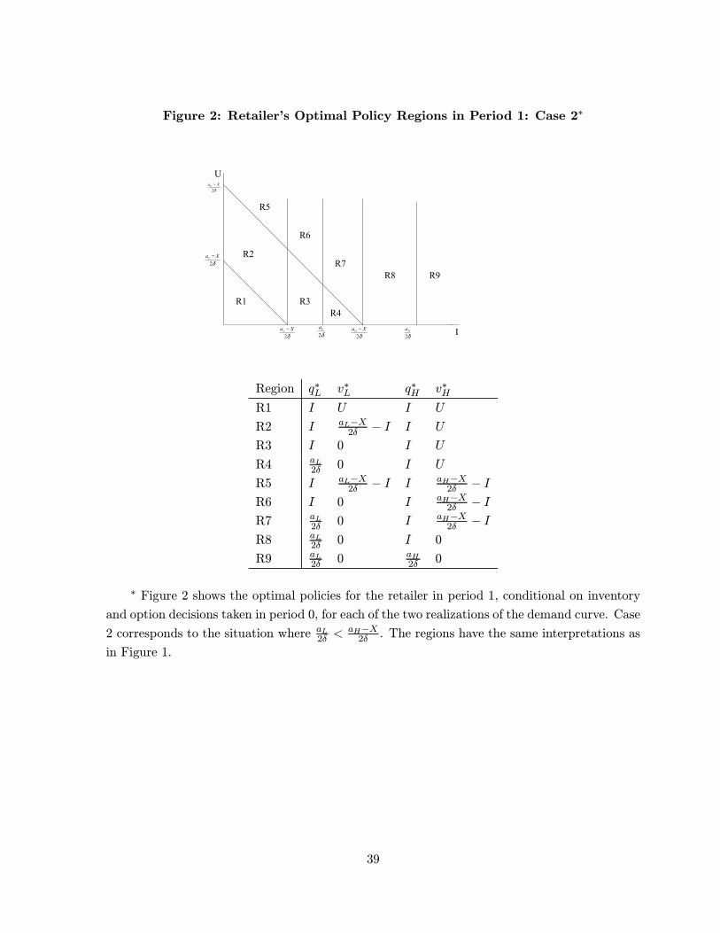
Figure 2: Retailer�s Optimal Policy Regions in Period 1: Case 2∗

δ2XaL −

δ2XaH −

δ2La

δ2Ha

δ2XaL −

δ2XaH −

I

U

R1

R2

R5

R3

R6

R7R8

R4

R9

Region q∗L v∗L q∗H v∗HR1 I U I U

R2 I aL−X2δ − I I U

R3 I 0 I U

R4 aL2δ 0 I U

R5 I aL−X2δ − I I aH−X

2δ − IR6 I 0 I aH−X

2δ − IR7 aL

2δ 0 I aH−X2δ − I

R8 aL2δ 0 I 0

R9 aL2δ 0 aH

2δ 0

∗ Figure 2 shows the optimal policies for the retailer in period 1, conditional on inventoryand option decisions taken in period 0, for each of the two realizations of the demand curve. Case

2 corresponds to the situation where aL2δ <

aH−X2δ . The regions have the same interpretations as

in Figure 1.

39

Figure 3: Equilibrium Wholesale Price∗

1.8

1.85

1.9

1.95

2

Price

0.5 1 1.5 2 2.5Volatility

∗Figure 3 shows the behavior of the wholesale price as the volatility of the demand curveincreases. The solid (dashed) line corresponds to the price when options (no options) are used.

The Þgure illustrates that with options the wholesale price is never lower than the price without

options. The intercept α of the demand curve follows a uniform distribution with mean µ and

variance σ2A. The case parameters for the problem are : δ = 0.5, B0 = 0.8, µ = 5,X = 2.5.

40

Figure 4: Variance of Equilibrium Retail Price∗

0

1

2

3

4

5

Variance

0.5 1 1.5 2 2.5Volatility

∗Figure 4 shows the variance of the retail price as the volatility of the demand curve increases.The solid (dashed) line corresponds to the price when options (no options) are used. The Þgure

illustrates that with options the volatility of the retail price is reduced compared to the case

without options. The intercept α of the demand curve follows a uniform distribution with mean

µ and variance σ2A. The case parameters for the problem are : δ = 0.5, B0 = 0.8, µ = 5,X = 2.5.

41

Figure 5a: Project Value for Manufacturer ∗

5

5.5

6

Value

1 2Volatility

∗Figure 5a shows the net present value of the project for the manufacturer as the volatilityof the demand curve increases. The solid (dashed) line corresponds to the price when options

(no options) are used. The Þgure illustrates that the project value for the manufacturer is

increasing in σA. Further, the value for the manufacturer is always higher when options are

offered. The difference between the two curves, which denotes the value of the options program

for the manufacturer, is increasing as the volatility of the demand curve increases. The intercept

α of the demand curve follows a uniform distribution with mean µ and variance σ2A. The case

parameters for the problem are : δ = 0.5, B0 = 0.8, µ = 5,X = 2.5.

42

Figure 5b: Project Value for Retailer ∗

2.6

2.8

3

3.2

Value

0.5 1 1.5 2 2.5Volatility

∗Figure 5b shows the net present value of the project for the retailer as the volatility ofthe demand curve increases. The solid (dashed) line corresponds to the price when options

(no options) are used. The Þgure illustrates that the project value for the retailer is increasing

in σA. In addition, the option program is beneÞcial for the retailer only when the volatility

of the demand curve is below a threshold. The intercept α of the demand curve follows a

uniform distribution with mean µ and variance σ2A. The case parameters for the problem are :

δ = 0.5, B0 = 0.8, µ = 5, X = 2.5.

43