Embed Size (px)
DESCRIPTION
calculadora de la distribucion de probabilidad gamma
Citation preview

The user enters values in column B. The worksheet calculates the remaining values
Value of Underlying Asset $50.0000Exercise Price $45.0000
T-bill rate 5.0000% Enter the continuously compounded annual rate as a decimal fraction. The value is displayed as a percentage.Time remaining 0.1644 Enter time in years. This value may be a fraction, such as 30/365 (type the following: =30/365).
Standard Deviation 20.0000% Enter as decimal fraction. The value is displayed as a percentage.
The following values are computed by the worksheet:
Value of Call Option: $5.5085 DeltaGamma
Value of Put Option: $0.1402 RhoTheta
PV of Exercise Price $44.63 Vegad(1) 1.4412325545971d(2) 1.3601440691892
N(d1) 0.9252N(d2) 0.9131
This worksheet calculates the value of call or put options using the Black/Scholes model.
In the case of a call option, the choice is to buy the underlying asset for the exercise price stated in the contract.
In the case of a put option, the choice is to sell the underlying asset for the exercise price stated in the contract.
In either case, the appropriate action can be chosen on the expiration date of the option.

The user enters values in column B. The worksheet calculates the remaining values
Enter the continuously compounded annual rate as a decimal fraction. The value is displayed as a percentage.Enter time in years. This value may be a fraction, such as 30/365 (type the following: =30/365).Enter as decimal fraction. The value is displayed as a percentage.
0.92520.03486.6992
-3.77912.8626

The user enters values in column B. The worksheet calculates the remaining values
Value of Underlying Asset $50.0000Exercise Price $45.0000
Market premium of call option 6.0000T-bill rate 5.0000% Enter the continuously compounded annual rate as a decimal fraction. The value is displayed as a percentage.
Time remaining 0.2466 Enter time in years. This value may be a fraction, such as 30/365 (type the following: =30/365).Estimated Standard Deviation 23.4674% Make an initial guess to start the program. Enter as decimal fraction. The value is displayed as a percentage.
The following values are computed by the worksheet:
Revised Implied Standard Deviation 23.4674% Press the ""Calculate ISD" button
Model Value of Call Option: $6.0000
Model Value of Put Option: $0.4486
PV of Exercise Price $44.45d(1) 1.0682094538658d(2) 0.9516789751623
N(d1) 0.8573N(d2) 0.8294
This worksheet calculates the implied standard deviation of call options using the Black/Scholes model.
In the case of a call option, the choice is to buy the underlying asset for the exercise price stated in the contract.
To use this worksheet, enter the values for the underlying asset, the exercise price, the market premium for the call option, the T-bill rate, the time remaining until expiration, and an initial estimate of the standard deviation.
Then press the "Calculate ISD" button. The worksheet will revise until the "Estimated Standard Deviation" matches the "Revised Implied Standard Deviation." Alternatively, you can press the "Command," "Option," and "s" keys simultaneously in order to launch the iterative process.
If put/call parity is violated, then the "Estimated Standard Deviation" will not match the "Revised Implied Standard Deviation." In extreme cases an error notification will appear.
If you did not enable macros when you opened this workbook, the button won't function. You can still work the calculation by using the "Revised Implied Standard Deviation" as a guide for making new entries in the "Estimated Standard Deviation." You should be able to get close in four to five repetitions.
The user enters values in column B. The worksheet calculates the remaining values
Enter the continuously compounded annual rate as a decimal fraction. The value is displayed as a percentage.Enter time in years. This value may be a fraction, such as 30/365 (type the following: =30/365).Make an initial guess to start the program. Enter as decimal fraction. The value is displayed as a percentage.
The following values are computed by the worksheet:
Delta 0.8573Gamma 0.0387
Rho 9.0898Theta -4.5074Vega 5.5985
This worksheet calculates the implied standard deviation of call options using the Black/Scholes model.
In the case of a call option, the choice is to buy the underlying asset for the exercise price stated in the contract.
To use this worksheet, enter the values for the underlying asset, the exercise price, the market premium for the call option, the T-bill rate, the time remaining until expiration, and an initial estimate of the standard deviation.
Then press the "Calculate ISD" button. The worksheet will revise until the "Estimated Standard Deviation" matches the "Revised Implied Standard Deviation." Alternatively, you can press the "Command," "Option," and "s" keys simultaneously in order to launch the iterative process.
If put/call parity is violated, then the "Estimated Standard Deviation" will not match the "Revised Implied Standard Deviation." In extreme cases an error notification will appear.
If you did not enable macros when you opened this workbook, the button won't function. You can still work the calculation by using the "Revised Implied Standard Deviation" as a guide for making new entries in the "Estimated Standard Deviation." You should be able to get close in four to five repetitions.

The user enters values in column B. The worksheet calculates the remaining values
Value of Underlying Asset $50.0000Exercise Price $45.0000
Market premium of put option 1.1000T-bill rate 5.0000% Enter the continuously compounded annual rate as a decimal fraction. The value is displayed as a percentage.
Time remaining 0.2466 Enter time in years. This value may be a fraction, such as 30/365 (type the following: =30/365).Estimated Standard Deviation 33.4423% Make an initial guess to start the program. Enter as decimal fraction. The value is displayed as a percentage.
The following values are computed by the worksheet:
Revised Implied Standard Deviation 33.4423% Press the ""Calculate ISD" button
Model Value of Call Option: $6.6514
Model Value of Put Option: $1.1000
PV of Exercise Price $44.45d(1) 0.7917359905958d(2) 0.6256734877254
N(d1) 0.7857N(d2) 0.7342
This worksheet calculates the implied standard deviation of put options using the Black/Scholes model.
In the case of a call option, the choice is to buy the underlying asset for the exercise price stated in the contract.
To use this worksheet, enter the values for the underlying asset, the exercise price, the market premium for the call option, the T-bill rate, the time remaining until expiration, and an initial estimate of the standard deviation.
Then press the "Calculate ISD" button. The worksheet will revise until the "Estimated Standard Deviation" matches the "Revised Implied Standard Deviation." Alternatively, you can press the "Command," "Option," and "s" keys simultaneously in order to launch the iterative process.
If you did not enable macros when you opened this workbook, the button won't function. You can still work the calculation by using the "Revised Implied Standard Deviation" as a guide for making new entries in the "Estimated Standard Deviation." You should be able to get close in four to five repetitions.

The user enters values in column B. The worksheet calculates the remaining values
Enter the continuously compounded annual rate as a decimal fraction. The value is displayed as a percentage.Enter time in years. This value may be a fraction, such as 30/365 (type the following: =30/365).Make an initial guess to start the program. Enter as decimal fraction. The value is displayed as a percentage.
The following values are computed by the worksheet:
Delta 0.7857Gamma 0.0351
Rho 8.0472Theta -6.5415Vega 7.2400
This worksheet calculates the implied standard deviation of put options using the Black/Scholes model.
In the case of a call option, the choice is to buy the underlying asset for the exercise price stated in the contract.
To use this worksheet, enter the values for the underlying asset, the exercise price, the market premium for the call option, the T-bill rate, the time remaining until expiration, and an initial estimate of the standard deviation.
Then press the "Calculate ISD" button. The worksheet will revise until the "Estimated Standard Deviation" matches the "Revised Implied Standard Deviation." Alternatively, you can press the "Command," "Option," and "s" keys simultaneously in order to launch the iterative process.
If you did not enable macros when you opened this workbook, the button won't function. You can still work the calculation by using the "Revised Implied Standard Deviation" as a guide for making new entries in the "Estimated Standard Deviation." You should be able to get close in four to five repetitions.

The user enters values in column B. The worksheet calculates the remaining values
Value of First Asset $4,000.0000Value of Second Asset $3,000.0000
Time remaining 1.0000 Enter time in years. This value may be a fraction, such as 30/365 (type =30/365).Standard Deviation of the First Asset 40.0000% Enter as decimal fraction. The value will be displayed as a percentage.
Standard Deviation of the Second Asset 20.0000% Enter as decimal fraction. The value will be displayed as a percentage.Correlation of returns for asset one and asset two 0.5000 Enter as decimal fraction. The range for this value is from -1 to +1.
The following values are computed by the worksheet:
Value of Call Option: $1,135.4454
Value of Put Option: $135.4454
Variance of the Price Ratio, Asset1/Asset2 12.0000%Standard Deviation of the Price Ratio, Asset1/Asset2 34.6410%
d(1) 1.0036716906122d(2) 0.6572615290984
N(d1) 0.8422N(d2) 0.7445
This worksheet calculates the value of an option to exchange one asset for another.
In the case of a call option, the choice is to give up the second asset in order to receive the first asset.
In the case of a put option, the choice is to give the first asset and receive the second asset.
The model used here was first published by William Margrabe.

The user enters values in column B. The worksheet calculates the remaining values
Enter time in years. This value may be a fraction, such as 30/365 (type =30/365).Enter as decimal fraction. The value will be displayed as a percentage.Enter as decimal fraction. The value will be displayed as a percentage.Enter as decimal fraction. The range for this value is from -1 to +1.
The following values are computed by the worksheet:
This worksheet calculates the value of an option to exchange one asset for another.
In the case of a call option, the choice is to give up the second asset in order to receive the first asset.
In the case of a put option, the choice is to give the first asset and receive the second asset.
The model used here was first published by William Margrabe.

The user enters values in column B. The worksheet calculates the remaining values
Value of Underlying Asset $50.0000Exercise Price $50.0000
T-bill rate 5.0000% Enter the continuously compounded annual rate as a decimal fraction. The value is displayed as a percentage.Time remaining 0.2466 Enter time in years. This value may be a fraction, such as 30/365 (type the following: =30/365).
Standard Deviation 20.0000% Enter as decimal fraction. The value is displayed as a percentage.
The following values are computed by the worksheet:
Value of Call Option: $2.2895 Delta of covered call position:
Value of Covered Call position: $47.7105
PV of Exercise Price $49.39d(1) 0.1737972366065d(2) 0.0744845299742
N(d1) 0.5690N(d2) 0.5297
This worksheet calculates the value of a covered call position using the Black/Scholes model.
In the case of a covered call, the investor buys the underlying and simultaneously sells a call option. The result is lower investment outlay and reduced delta, compared with a naked position in the underlyling.
The user enters values in column B. The worksheet calculates the remaining values
Enter the continuously compounded annual rate as a decimal fraction. The value is displayed as a percentage.Enter time in years. This value may be a fraction, such as 30/365 (type the following: =30/365).Enter as decimal fraction. The value is displayed as a percentage.
0.4310

The user enters values in column B. The worksheet calculates the remaining values
Value of Underlying Asset $50.0000Exercise Price $50.0000
T-bill rate 5.0000% Enter the continuously compounded annual rate as a decimal fraction. The value is displayed as a percentage.Time remaining 0.2466 Enter time in years. This value may be a fraction, such as 30/365 (type the following: =30/365).
Standard Deviation 20.0000% Enter as decimal fraction. The value is displayed as a percentage.
The following values are computed by the worksheet:
Value of Put Option: $1.6769 Delta of protective put position:
Value of Protective Put position: $51.6769
PV of Exercise Price $49.39d(1) 0.1737972366065d(2) 0.0744845299742
N(d1) 0.5690N(d2) 0.5297
This worksheet calculates the value of a protective put position using the Black/Scholes model.
In the case of a protective put, the investor buys the underlying and simultaneously buys a put option. The result is higher investment outlay and reduced delta, compared with a naked position in the underlyling.
Note: Delta for the protective put position is the same as the delta for the call

The user enters values in column B. The worksheet calculates the remaining values
Enter the continuously compounded annual rate as a decimal fraction. The value is displayed as a percentage.Enter time in years. This value may be a fraction, such as 30/365 (type the following: =30/365).Enter as decimal fraction. The value is displayed as a percentage.
0.5690

The user enters values in column B. The worksheet calculates the remaining values
Value of Underlying Asset $45.0000Exercise Price $45.0000
T-bill rate 5.0000% Enter the continuously compounded annual rate as a decimal fraction. The value is displayed as a percentage.Time remaining 0.2466 Enter time in years. This value may be a fraction, such as 30/365 (type the following: =30/365).
Standard Deviation 20.0000% Enter as decimal fraction. The value is displayed as a percentage.
The following values are computed by the worksheet:
Value of call: $2.0606 Delta for the straddleValue of put: $1.5092
Value of Straddle: $3.5697
PV of Exercise Price $44.45d(1) 0.1737972366065d(2) 0.0744845299742
N(d1) 0.5690N(d2) 0.5297
This worksheet calculates the value of a Straddle using the Black/Scholes model.
A Straddle is made from calls and puts with the same exercise price, the same underlying, and the same expiration. A long straddle is long one call and long one put.
When the stock price is above the present value of the exercise price, the delta is positive. As the stock rises from there, the value of the straddle increases, and the delta rapidly grows toward +1.
If the stock moves below the present value of the exercise price, delta soon becomes negative and shrinks rapidly as the value of the underlying declines (toward –1). As the stock price falls over this range, the value of the straddle increases.
A short straddle is short one call and short one put. Going short provides an inflow at the time the straddle is established, and reverses the delta scenarios.

The user enters values in column B. The worksheet calculates the remaining values
Enter the continuously compounded annual rate as a decimal fraction. The value is displayed as a percentage.Enter time in years. This value may be a fraction, such as 30/365 (type the following: =30/365).Enter as decimal fraction. The value is displayed as a percentage.
0.1380
This worksheet calculates the value of a Straddle using the Black/Scholes model.
A Straddle is made from calls and puts with the same exercise price, the same underlying, and the same expiration. A long straddle is long one call and long one put.
When the stock price is above the present value of the exercise price, the delta is positive. As the stock rises from there, the value of the straddle increases, and the delta rapidly grows toward +1.
If the stock moves below the present value of the exercise price, delta soon becomes negative and shrinks rapidly as the value of the underlying declines (toward –1). As the stock price falls over this range, the value of the straddle increases.
A short straddle is short one call and short one put. Going short provides an inflow at the time the straddle is established, and reverses the delta scenarios.

The user enters values in column B. The worksheet calculates the remaining values
Value of Underlying Asset $47.5000Exercise Price $45.0000
T-bill rate 5.0000% Enter the continuously compounded annual rate as a decimal fraction. The value is displayed as a percentage.Time remaining 0.2466 Enter time in years. This value may be a fraction, such as 30/365 (type the following: =30/365).
Standard Deviation 20.0000% Enter as decimal fraction. The value is displayed as a percentage.
The following values are computed by the worksheet:
Value of call: $3.7384 Delta for the strapValue of put: $0.6870
Value of Strap: $8.1637
PV of Exercise Price $44.45d(1) 0.7182111701675d(2) 0.6188984635353
N(d1) 0.7637N(d2) 0.7320
This worksheet calculates the value of a Strap using the Black/Scholes model.
A Strap is a straddle augmented on the bullish side. It is made from calls and puts with the same exercise price, the same underlying, and the same expiration. A long strap is long two calls and long one put.
When the stock price is above the present value of the exercise price, the delta is positive. As the stock rises from there, the value of the strap increases, and the delta rapidly grows toward +2.
If the stock moves below the present value of the exercise price, delta soon becomes negative and shrinks rapidly as the value of the underlying declines (toward –1). As the stock price falls over this range, the value of the strap increases.
A short strap is short two calls and short one put. Going short provides an inflow at the time the strap is established, and reverses the delta scenarios.

The user enters values in column B. The worksheet calculates the remaining values
Enter the continuously compounded annual rate as a decimal fraction. The value is displayed as a percentage.Enter time in years. This value may be a fraction, such as 30/365 (type the following: =30/365).Enter as decimal fraction. The value is displayed as a percentage.
1.2911
This worksheet calculates the value of a Strap using the Black/Scholes model.
A Strap is a straddle augmented on the bullish side. It is made from calls and puts with the same exercise price, the same underlying, and the same expiration. A long strap is long two calls and long one put.
When the stock price is above the present value of the exercise price, the delta is positive. As the stock rises from there, the value of the strap increases, and the delta rapidly grows toward +2.
If the stock moves below the present value of the exercise price, delta soon becomes negative and shrinks rapidly as the value of the underlying declines (toward –1). As the stock price falls over this range, the value of the strap increases.
A short strap is short two calls and short one put. Going short provides an inflow at the time the strap is established, and reverses the delta scenarios.

The user enters values in column B. The worksheet calculates the remaining values
Value of Underlying Asset $46.0000Exercise Price $45.0000
T-bill rate 5.0000% Enter the continuously compounded annual rate as a decimal fraction. The value is displayed as a percentage.Time remaining 0.2466 Enter time in years. This value may be a fraction, such as 30/365 (type the following: =30/365).
Standard Deviation 20.0000% Enter as decimal fraction. The value is displayed as a percentage.
The following values are computed by the worksheet:
Value of call: $2.6725 Delta for the strapValue of put: $1.1211
Value of Strip: $4.9146
PV of Exercise Price $44.45d(1) 0.3951073535501d(2) 0.2957946469178
N(d1) 0.6536N(d2) 0.6163
This worksheet calculates the value of a Strip using the Black/Scholes model.
A Strip is a straddle augmented on the bearish side. It is made from calls and puts with the same exercise price, the same underlying, and the same expiration. A long strip is long one call and long two puts.
When the stock price is below the exercise price, the delta is negative. As the stock falls from there, the value of the strip increases, and the delta rapidly grows toward –2.
If the stock moves above the exercise price, delta soon becomes positive and grows rapidly as the value of the underlying rises (toward +1). As the stock price rises over this range, the value of the strip increases.
A short strip is short one call and short two puts. Going short provides an inflow at the time the strip is established, and reverses the delta scenarios.

The user enters values in column B. The worksheet calculates the remaining values
Enter the continuously compounded annual rate as a decimal fraction. The value is displayed as a percentage.Enter time in years. This value may be a fraction, such as 30/365 (type the following: =30/365).Enter as decimal fraction. The value is displayed as a percentage.
-0.0391
This worksheet calculates the value of a Strip using the Black/Scholes model.
A Strip is a straddle augmented on the bearish side. It is made from calls and puts with the same exercise price, the same underlying, and the same expiration. A long strip is long one call and long two puts.
When the stock price is below the exercise price, the delta is negative. As the stock falls from there, the value of the strip increases, and the delta rapidly grows toward –2.
If the stock moves above the exercise price, delta soon becomes positive and grows rapidly as the value of the underlying rises (toward +1). As the stock price rises over this range, the value of the strip increases.
A short strip is short one call and short two puts. Going short provides an inflow at the time the strip is established, and reverses the delta scenarios.

The user enters values in column B. The worksheet calculates the remaining values
Value of Underlying Asset $47.50001st Exercise Price $45.0000
2nd Exercise Price $50.0000T-bill rate 5.0000% Enter the continuously compounded annual rate as a decimal fraction. The value is displayed as a percentage.
Time remaining 0.2466 Enter time in years. This value may be a fraction, such as 30/365 (type the following: =30/365).Standard Deviation 20.0000% Enter as decimal fraction. The value is displayed as a percentage.
The following values are computed by the worksheet:
Value of put at 1st exercise price: $0.6870 Delta for the spreadValue of call at 2nd exercise price: $1.1205
Value of Strangle: $1.8075
PV of Exercise Price $44.45 $49.39d(1) 0.7182111701675 -0.34268546d(2) 0.6188984635353 -0.44199817
N(d1) 0.7637 0.3659N(d2) 0.7320 0.3292
This worksheet calculates the value of a Strangle using the Black/Scholes model.
A Strangle is made from calls and puts with two different exercise prices, with the price of the underlying between them (say, exercise prices at 45 & 50, with the underlying at 47.50). Both of the options have the same underlying and the same expiration.
A long strangle is long one call at the higher exercise price and long one put at the lower exercise price (both options out-of-the-money). With both options out-of-the-money, the cost of entry is relatively low.
Over much of the space between exercise prices, the delta is positive. If the stock moves above the 2nd exercise price, delta is positive and grows rapidly larger (toward +1) as the value of the underlying rises. If the stock moves below the 1st exercise price, delta is negative and shrinks rapidly as the value of the underlying declines (toward –1).
A short strangle is short one call at the higher exercise price, and long one put at the lower exercise price. Going short provides an inflow at the time the spread is established, and reverses the delta scenarios.

The user enters values in column B. The worksheet calculates the remaining values
Enter the continuously compounded annual rate as a decimal fraction. The value is displayed as a percentage.Enter time in years. This value may be a fraction, such as 30/365 (type the following: =30/365).Enter as decimal fraction. The value is displayed as a percentage.
0.1296
This worksheet calculates the value of a Strangle using the Black/Scholes model.
A Strangle is made from calls and puts with two different exercise prices, with the price of the underlying between them (say, exercise prices at 45 & 50, with the underlying at 47.50). Both of the options have the same underlying and the same expiration.
A long strangle is long one call at the higher exercise price and long one put at the lower exercise price (both options out-of-the-money). With both options out-of-the-money, the cost of entry is relatively low.
Over much of the space between exercise prices, the delta is positive. If the stock moves above the 2nd exercise price, delta is positive and grows rapidly larger (toward +1) as the value of the underlying rises. If the stock moves below the 1st exercise price, delta is negative and shrinks rapidly as the value of the underlying declines (toward –1).
A short strangle is short one call at the higher exercise price, and long one put at the lower exercise price. Going short provides an inflow at the time the spread is established, and reverses the delta scenarios.
The user enters values in column B. The worksheet calculates the remaining values
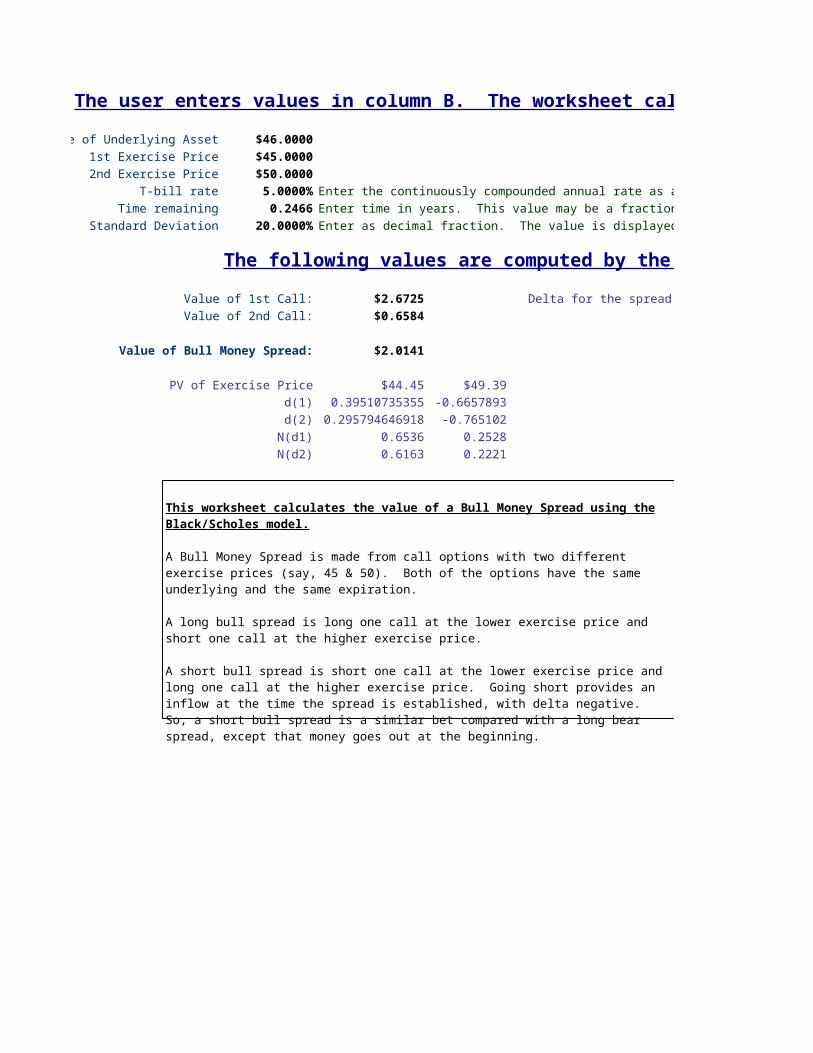
Value of Underlying Asset $46.00001st Exercise Price $45.0000
2nd Exercise Price $50.0000T-bill rate 5.0000% Enter the continuously compounded annual rate as a decimal fraction. The value is displayed as a percentage.
Time remaining 0.2466 Enter time in years. This value may be a fraction, such as 30/365 (type the following: =30/365).Standard Deviation 20.0000% Enter as decimal fraction. The value is displayed as a percentage.
The following values are computed by the worksheet:
Value of 1st Call: $2.6725 Delta for the spreadValue of 2nd Call: $0.6584
Value of Bull Money Spread: $2.0141
PV of Exercise Price $44.45 $49.39d(1) 0.3951073535501 -0.66578928d(2) 0.2957946469178 -0.76510198
N(d1) 0.6536 0.2528N(d2) 0.6163 0.2221
This worksheet calculates the value of a Bull Money Spread using the Black/Scholes model.
A Bull Money Spread is made from call options with two different exercise prices (say, 45 & 50). Both of the options have the same underlying and the same expiration.
A long bull spread is long one call at the lower exercise price and short one call at the higher exercise price.
A short bull spread is short one call at the lower exercise price and long one call at the higher exercise price. Going short provides an inflow at the time the spread is established, with delta negative. So, a short bull spread is a similar bet compared with a long bear spread, except that money goes out at the beginning.
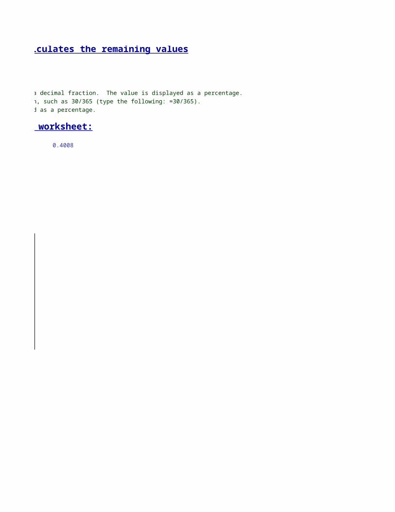
The user enters values in column B. The worksheet calculates the remaining values
Enter the continuously compounded annual rate as a decimal fraction. The value is displayed as a percentage.Enter time in years. This value may be a fraction, such as 30/365 (type the following: =30/365).Enter as decimal fraction. The value is displayed as a percentage.
0.4008
This worksheet calculates the value of a Bull Money Spread using the Black/Scholes model.
A Bull Money Spread is made from call options with two different exercise prices (say, 45 & 50). Both of the options have the same underlying and the same expiration.
A long bull spread is long one call at the lower exercise price and short one call at the higher exercise price.
A short bull spread is short one call at the lower exercise price and long one call at the higher exercise price. Going short provides an inflow at the time the spread is established, with delta negative. So, a short bull spread is a similar bet compared with a long bear spread, except that money goes out at the beginning.

The user enters values in column B. The worksheet calculates the remaining values
Value of Underlying Asset $46.00001st Exercise Price $45.0000
2nd Exercise Price $50.0000T-bill rate 5.0000% Enter the continuously compounded annual rate as a decimal fraction. The value is displayed as a percentage.
Time remaining 0.2466 Enter time in years. This value may be a fraction, such as 30/365 (type the following: =30/365).Standard Deviation 20.0000% Enter as decimal fraction. The value is displayed as a percentage.
The following values are computed by the worksheet:
Value of Put at 1st exercise price: $1.1211 Delta for the spreadValue of Call at 2nd exercise price: $0.6584
Value of Collar: $46.4627
PV of Exercise Price $44.45 $49.39d(1) 0.3951073535501 -0.66578928d(2) 0.2957946469178 -0.76510198
N(d1) 0.6536 0.2528N(d2) 0.6163 0.2221
This worksheet calculates the value of a Collara using the Black/Scholes model.
A Collar is made from calls and puts with two different exercise prices (say, 45 & 50). Both of the options have the same underlying and the same expiration.
A long collar is long the underlying, long one put at the lower exercise price and short one call at the higher exercise price. Thus the holder owns the underlying asset, but has locked in a minimum value and has accepted a maximum value.
A collar is similar to a bull money spread because (by put-call parity) a collar equals a risk-free bond with face value of the lower exercise price, plus a long bull spread ( the bull spread is long a call at the lower exercise price and a short call at the higher exercise price). So, the delta for a collar is the same as the delta for a bull money spread.

The user enters values in column B. The worksheet calculates the remaining values
Enter the continuously compounded annual rate as a decimal fraction. The value is displayed as a percentage.Enter time in years. This value may be a fraction, such as 30/365 (type the following: =30/365).Enter as decimal fraction. The value is displayed as a percentage.
0.4008
This worksheet calculates the value of a Collara using the Black/Scholes model.
A Collar is made from calls and puts with two different exercise prices (say, 45 & 50). Both of the options have the same underlying and the same expiration.
A long collar is long the underlying, long one put at the lower exercise price and short one call at the higher exercise price. Thus the holder owns the underlying asset, but has locked in a minimum value and has accepted a maximum value.
A collar is similar to a bull money spread because (by put-call parity) a collar equals a risk-free bond with face value of the lower exercise price, plus a long bull spread ( the bull spread is long a call at the lower exercise price and a short call at the higher exercise price). So, the delta for a collar is the same as the delta for a bull money spread.

The user enters values in column B. The worksheet calculates the remaining values
Value of Underlying Asset $46.00001st Exercise Price $45.0000
2nd Exercise Price $50.0000T-bill rate 5.0000% Enter the continuously compounded annual rate as a decimal fraction. The value is displayed as a percentage.
Time remaining 0.2466 Enter time in years. This value may be a fraction, such as 30/365 (type the following: =30/365).Standard Deviation 20.0000% Enter as decimal fraction. The value is displayed as a percentage.
The following values are computed by the worksheet:
Value of 1st Put: $1.1211 Delta for the spreadValue of 2nd Put: $4.0457
Value of Bear Money Spread: $2.9246
PV of Exercise Price $44.45 $49.39d(1) 0.3951073535501 -0.66578928d(2) 0.2957946469178 -0.76510198
N(d1) 0.6536 0.2528N(d2) 0.6163 0.2221
This worksheet calculates the value of a Bear Money Spread using the Black/Scholes model.
A Bear Money Spread is made from put options with two different exercise prices (say, 45 & 50). Both of the options have the same underlying and the same expiration.
A long bear spread is long one put at the higher exercise price and short one put at the lower exercise price. The delta for a long bear spread is the negative of the delta for a long bull spread.
A short bear spread is short one put at the higher exercise price and long one put at the lower exercise price. Going short provides an inflow at the time the spread is established, with delta positive. So, a short bear spread is a similar bet compared with a long bull spread, except that money comes in at the beginning as well as (possibly) at the end. The delta for a short bear spread is the same as the delta for a long bull spread.

The user enters values in column B. The worksheet calculates the remaining values
Enter the continuously compounded annual rate as a decimal fraction. The value is displayed as a percentage.Enter time in years. This value may be a fraction, such as 30/365 (type the following: =30/365).Enter as decimal fraction. The value is displayed as a percentage.
-0.4008
This worksheet calculates the value of a Bear Money Spread using the Black/Scholes model.
A Bear Money Spread is made from put options with two different exercise prices (say, 45 & 50). Both of the options have the same underlying and the same expiration.
A long bear spread is long one put at the higher exercise price and short one put at the lower exercise price. The delta for a long bear spread is the negative of the delta for a long bull spread.
A short bear spread is short one put at the higher exercise price and long one put at the lower exercise price. Going short provides an inflow at the time the spread is established, with delta positive. So, a short bear spread is a similar bet compared with a long bull spread, except that money comes in at the beginning as well as (possibly) at the end. The delta for a short bear spread is the same as the delta for a long bull spread.

The user enters values in column B. The worksheet calculates the remaining values
Value of Underlying Asset $45.60001st Exercise Price $45.0000
T-bill rate 5.0000% Enter the continuously compounded annual rate as a decimal fraction. The value is displayed as a percentage.Shorter Time remaining 0.1644 Enter time in years. This value may be a fraction, such as 30/365 (type the following: =30/365).Longer Time remaining 0.2466 Enter time in years. This value may be a fraction, such as 30/365 (type the following: =30/365).
Standard Deviation 20.0000% Enter as decimal fraction. The value is displayed as a percentage.
The following values are computed by the worksheet:
Value of 1st Call: $1.9940 Delta for the spreadValue of 2nd Call: $2.4176
Value of Calendar Spread: $0.4235
PV of Exercise Price $44.63 $44.45d(1) 0.3052477295706 0.30716614d(2) 0.2241592441626 0.207853433
N(d1) 0.6199 0.6206N(d2) 0.5887 0.5823
This worksheet calculates the value of a Calendar Spread using the Black/Scholes model.
A Calendar Spread is made from call options with two different expiration dates (say, 60 days & 90 days). Both of the options have the same underlying and the same exercise price.
A long calendar spread is long one call at the longer time and short one call at the lesser time. It's delta is positive when the options are out-of-the-money, and turns negative soon after the options move into the money. The value of the calendar spread is highest when the options are near the money.
A short calendar spread is short one call at the longer time and long one call at the lesser time. It's delta follows the opposite scenario compared with the long spread.

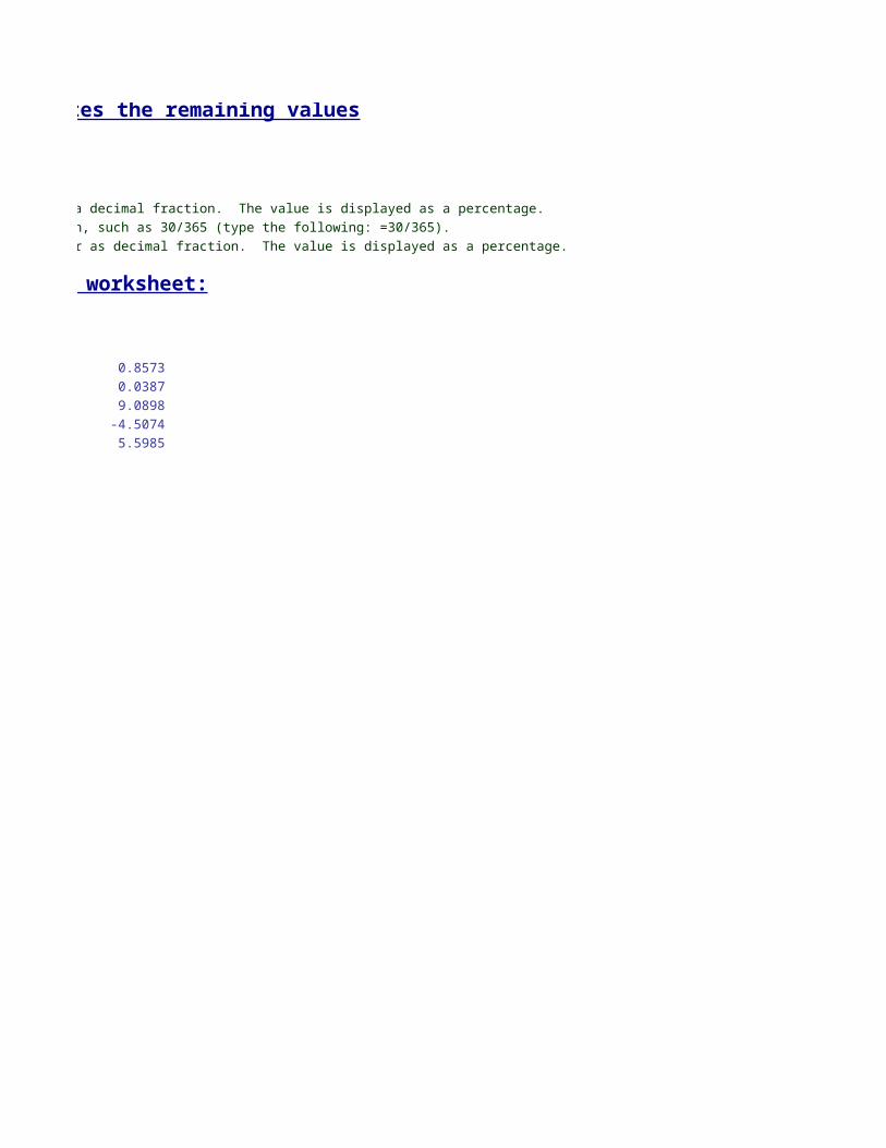
The user enters values in column B. The worksheet calculates the remaining values
Enter the continuously compounded annual rate as a decimal fraction. The value is displayed as a percentage.Enter time in years. This value may be a fraction, such as 30/365 (type the following: =30/365).Enter time in years. This value may be a fraction, such as 30/365 (type the following: =30/365).Enter as decimal fraction. The value is displayed as a percentage.
0.0007
This worksheet calculates the value of a Calendar Spread using the Black/Scholes model.
A Calendar Spread is made from call options with two different expiration dates (say, 60 days & 90 days). Both of the options have the same underlying and the same exercise price.
A long calendar spread is long one call at the longer time and short one call at the lesser time. It's delta is positive when the options are out-of-the-money, and turns negative soon after the options move into the money. The value of the calendar spread is highest when the options are near the money.
A short calendar spread is short one call at the longer time and long one call at the lesser time. It's delta follows the opposite scenario compared with the long spread.

The user enters values in column B. The worksheet calculates the remaining values
Value of Underlying Asset $165.12501st Exercise Price $165.0000
2nd Exercise Price $170.0000T-bill rate for shorter time 5.0300% Enter the continuously compounded annual rate as a decimal fraction. The value is displayed as a percentage.T-bill rate for longer time 5.7100% Enter the continuously compounded annual rate as a decimal fraction. The value is displayed as a percentage.
Shorter Time remaining 0.0877 Enter time in years. This value may be a fraction, such as 30/365 (type the following: =30/365).Longer Time remaining 0.2603 Enter time in years. This value may be a fraction, such as 30/365 (type the following: =30/365).
Standard Deviation 21.0000% Enter as decimal fraction. The value is displayed as a percentage.
The following values are computed by the worksheet:
Value of 1st Call: $8.3533 Delta for the spreadValue of 2nd Call: $2.4056
Value of Calendar Spread: $5.9477
PV of Exercise Price $162.57 $169.25d(1) 0.1993541981374 -0.36591847d(2) 0.092218386236 -0.42809806
N(d1) 0.5790 0.3572N(d2) 0.5367 0.3343
This worksheet calculates the value of a Diagonal Spread using the Black/Scholes model.
Sometimes option traders use a combination of a money spread and a calendar spread called a diagonal spread. This transaction involves the purchase of a call with a lower exercise price and a longer time to expiration combined with the sale of a call with a higher exercise price and a shorter time to expiration.

The user enters values in column B. The worksheet calculates the remaining values
Enter the continuously compounded annual rate as a decimal fraction. The value is displayed as a percentage.Enter the continuously compounded annual rate as a decimal fraction. The value is displayed as a percentage.Enter time in years. This value may be a fraction, such as 30/365 (type the following: =30/365).Enter time in years. This value may be a fraction, such as 30/365 (type the following: =30/365).Enter as decimal fraction. The value is displayed as a percentage.
0.2218
This worksheet calculates the value of a Diagonal Spread using the Black/Scholes model.
Sometimes option traders use a combination of a money spread and a calendar spread called a diagonal spread. This transaction involves the purchase of a call with a lower exercise price and a longer time to expiration combined with the sale of a call with a higher exercise price and a shorter time to expiration.
The user enters values in column B. The worksheet calculates the remaining values
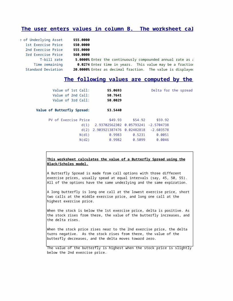
Value of Underlying Asset $55.00001st Exercise Price $50.0000
2nd Exercise Price $55.00003rd Exercise Price $60.0000
T-bill rate 5.0000% Enter the continuously compounded annual rate as a decimal fraction. The value is displayed as a percentage.Time remaining 0.0274 Enter time in years. This value may be a fraction, such as 30/365 (type the following: =30/365).
Standard Deviation 20.0000% Enter as decimal fraction. The value is displayed as a percentage.
The following values are computed by the worksheet:
Value of 1st Call: $5.0693 Delta for the spreadValue of 2nd Call: $0.7641Value of 3rd Call: $0.0029
Value of Butterfly Spread: $3.5440
PV of Exercise Price $49.93 $54.92 $59.92d(1) 2.9370256230202 0.057932412 -2.57047376d(2) 2.9039213874761 0.024828177 -2.60357799
N(d1) 0.9983 0.5231 0.0051N(d2) 0.9982 0.5099 0.0046
This worksheet calculates the value of a Butterfly Spread using the Black/Scholes model.
A Butterfly Spread is made from call options with three different exercise prices, usually spead at equal intervals (say, 45, 50, 55). All of the options have the same underlying and the same expiration.
A long butterfly is long one call at the lowest exercise price, short two calls at the middle exercise price, and long one call at the highest exercise price.
When the stock is below the 1st exercise price, delta is positive. As the stock rises from there, the value of the butterfly increases, and the delta rises.
When the stock price rises near to the 2nd exercise price, the delta turns negative. As the stock rises from there, the value of the butterfly decreases, and the delta moves toward zero.
The value of the butterfly is highest when the stock price is slightly below the 2nd exercise price.

The user enters values in column B. The worksheet calculates the remaining values
Enter the continuously compounded annual rate as a decimal fraction. The value is displayed as a percentage.Enter time in years. This value may be a fraction, such as 30/365 (type the following: =30/365).Enter as decimal fraction. The value is displayed as a percentage.
-0.0428

The user enters values in column B. The worksheet calculates the remaining values
Value of Underlying Asset $52.00001st Exercise Price $45.0000
2nd Exercise Price $50.00003rd Exercise Price $55.00004th Exercise Price $60.0000
T-bill rate 5.0000% Enter the continuously compounded annual rate as a decimal fraction. The value is displayed as a percentage.Time remaining 0.2466 Enter time in years. This value may be a fraction, such as 30/365 (type the following: =30/365).
Standard Deviation 20.0000% Enter as decimal fraction. The value is displayed as a percentage.
The following values are computed by the worksheet:
Value of 1st Call: $7.6676 Delta for the spreadValue of 2nd Call: $3.5782Value of 3rd Call: $1.1434Value of 4th Call: $0.2420
Value of Condor Spread: $3.1880
PV of Exercise Price $44.45 $49.39 $54.33 $59.26d(1) 1.629615265476 0.568718637 -0.3909791 -1.26711449d(2) 1.5303025588437 0.46940593 -0.49029181 -1.3664272
N(d1) 0.9484 0.7152 0.3479 0.1026N(d2) 0.9370 0.6806 0.3120 0.0859
This worksheet calculates the value of a Condor Spread using the Black/Scholes model.
A Condor Spread is a butterfly with extended wingspan (done by inserting a gap between the exercise prices of the two short calls). It is made from call options with four different exercise prices (say, 45, 50, 55, 60). All of the options have the same underlying and the same expiration.
A long condor is long one call at the lowest exercise price, short a call at each of the next two larger exercise prices, and long one call at the highest exercise price (say, long the 45, short the 50, short the 55, and long the 60).
In terms of delta, a condor is similar to a strangle.

The user enters values in column B. The worksheet calculates the remaining values
Enter the continuously compounded annual rate as a decimal fraction. The value is displayed as a percentage.Enter time in years. This value may be a fraction, such as 30/365 (type the following: =30/365).Enter as decimal fraction. The value is displayed as a percentage.
-0.0122
This worksheet calculates the value of a Condor Spread using the Black/Scholes model.
A Condor Spread is a butterfly with extended wingspan (done by inserting a gap between the exercise prices of the two short calls). It is made from call options with four different exercise prices (say, 45, 50, 55, 60). All of the options have the same underlying and the same expiration.
A long condor is long one call at the lowest exercise price, short a call at each of the next two larger exercise prices, and long one call at the highest exercise price (say, long the 45, short the 50, short the 55, and long the 60).
In terms of delta, a condor is similar to a strangle.

The user enters values in column B. The worksheet calculates the remaining values
Value of Underlying Asset $50.0000xercise Price for calls used as gamma hedge $50.0000
Exercise Price for calls used as delta hedge $45.0000T-bill rate 5.0000% Enter the continuously compounded annual rate as a decimal fraction. The value is displayed as a percentage.
e remaining for calls used as gamma hedge 0.0274 Enter time in years. This value may be a fraction, such as 30/365 (type the following: =30/365).ime remaining for calls used as delta hedge 0.1644 Enter time in years. This value may be a fraction, such as 30/365 (type the following: =30/365).
Standard Deviation 20.0000% Enter as decimal fraction. The value is displayed as a percentage.Shares of the underlying to be hedged 1,000 Enter the number of shares held. Positive sign indicates long, negative sign indicates short
The following values are computed by the worksheet:
Value of 1st Call: $0.6946 Delta of 1st optionValue of 2nd Call: $5.5085 Delta of 2nd option
Gamma of 1st optionValue of total position: $43,634.12 Gamma of 2nd option
PV of Exercise Price $49.93 $44.63d(1) 0.0579324122022 1.441232555d(2) 0.0248281766581 1.360144069
N(d1) 0.5231 0.9252N(d2) 0.5099 0.9131
This worksheet calculates the hedge ratios for a delta and gama neutral hedge, using the Black/Scholes model.
A delta and gamma neutral hedge uses two options to hedge the risks of a position in the underlying. The two options have the same underlying but different exercise prices or expiration dates.
Since gamma is greatest for calls that are near the money with a short time remaining until expiration, such options can be useful tools in the gamma portion of the hedge.
Since delta is greatest for in-the-money options, such options can be useful tools in the delta portion of the hedge.
The spreadsheet calculates the number of options necessary to complete the hedge (rounded to nearest whole number). It also shows the value of the total position, from which you can see that the hedge is not perfect (the value does fluctuate as the value of the underlying changes). Even so, the fluctuations are very much more gentle than with an unhedged position in the underlying.

The user enters values in column B. The worksheet calculates the remaining values
Enter the continuously compounded annual rate as a decimal fraction. The value is displayed as a percentage.Enter time in years. This value may be a fraction, such as 30/365 (type the following: =30/365).Enter time in years. This value may be a fraction, such as 30/365 (type the following: =30/365).Enter as decimal fraction. The value is displayed as a percentage.Enter the number of shares held. Positive sign indicates long, negative sign indicates short
The following values are computed by the worksheet:
Delta of 1st option 0.5231Delta of 2nd option 0.9252
Gamma of 1st option 0.2406Gamma of 2nd option 0.0348
170 Number of calls for gamma portion of the hedge-1,177 Number of calls to complete the delta portion of the hedge
0 Delta of hedge0 Gamma of hedge
This worksheet calculates the hedge ratios for a delta and gama neutral hedge, using the Black/Scholes model.
A delta and gamma neutral hedge uses two options to hedge the risks of a position in the underlying. The two options have the same underlying but different exercise prices or expiration dates.
Since gamma is greatest for calls that are near the money with a short time remaining until expiration, such options can be useful tools in the gamma portion of the hedge.
Since delta is greatest for in-the-money options, such options can be useful tools in the delta portion of the hedge.
The spreadsheet calculates the number of options necessary to complete the hedge (rounded to nearest whole number). It also shows the value of the total position, from which you can see that the hedge is not perfect (the value does fluctuate as the value of the underlying changes). Even so, the fluctuations are very much more gentle than with an unhedged position in the underlying.

The user enters values in column B. The worksheet calculates the remaining values
Value of Underlying Asset $1,224.3600 Enter today's value of the equity index that best fits the portfolio you wish to insureExercise Price $1,210.0000 Enter the floor value of the equity index that you wish to set as the insured level
T-bill rate 5.0000% Enter the continuously compounded annual rate as a decimal fraction. The value is displayed as a percentage.Time remaining 0.2466 Enter time in years. This value may be a fraction, such as 30/365 (type the following: =30/365).
Standard Deviation 17.5000% Enter as decimal fraction. The value is displayed as a percentage.
Dividend yield 3.00% Enter the dividend yield of the index as a decimal fraction"Shares" of the Index 21,000.00 Enter the number of "shares" in the index your portfolio contains (this is the total value of the portfolio divided by the level of the index on the first day of portfolio insurance)
Futures multiplier 250 Enter this value if you want to calculate a portfolio insurance strategy using futures contracts on the equity index
The following values are computed by the worksheet:
Value of Call Option: $53.0133 0.5778
Value of Put Option: $32.7009
PV of Bonds (adjusted for dividends) $1,204.05 20,453.71d(1) 0.2359656697152d(2) 0.1490670514119
N(d1) 0.5933N(d2) 0.5592
Shares of equity in the Insured Portfolio 12134.58 $14,857,094.62Number of Bonds in the Insured Portfolio 9014.98 $10,854,465.38
Number of index futures contracts -35.29 $25,711,560.00
$24,748,990.34
This worksheet calculates the proportions for establishing portfolio insurance strategies
Portfolio insurance is a dynamic strategy and requires frequent revision to keep up with changing equity values. The time remaining until expiration is the only thing that remains constant through the life of the insurance coverage. You choose this time horizon as part of the initial strategy. This worksheet helps only for the initial setup of the portfolio insurance strategy, not for revision of an established strategy. The option models in this worksheet are adjusted for dividends.
Through portfolio insurance, the investor creates portfolios with revised proportions of equity and bonds, creating a synthetic put option that protects the portfolio against loss. The revised portfolio responds to changes in the equity value the same way a portfolio of equity and puts would respond.
An alternative is to use futures contracts on the equity index in order to alter the response of the insured portfolio so that it responds to changes in the equity value the same way a portfolio of equity and puts would respond. The equity position remains unchanged, but the short futures position brings the delta of the insured portfolio toward the target level. The shortcoming is the lack of precision because fractional contracts are not available.
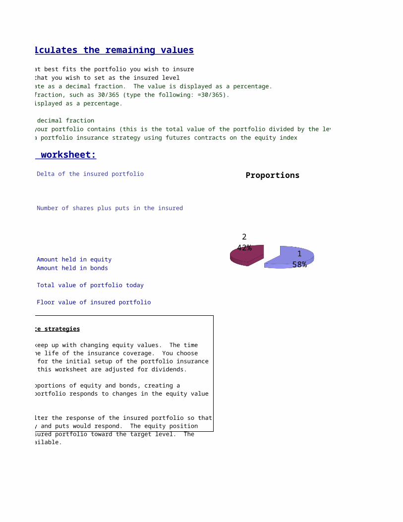
The user enters values in column B. The worksheet calculates the remaining values
Enter today's value of the equity index that best fits the portfolio you wish to insureEnter the floor value of the equity index that you wish to set as the insured levelEnter the continuously compounded annual rate as a decimal fraction. The value is displayed as a percentage.Enter time in years. This value may be a fraction, such as 30/365 (type the following: =30/365).Enter as decimal fraction. The value is displayed as a percentage.
Enter the dividend yield of the index as a decimal fractionEnter the number of "shares" in the index your portfolio contains (this is the total value of the portfolio divided by the level of the index on the first day of portfolio insurance)Enter this value if you want to calculate a portfolio insurance strategy using futures contracts on the equity index
Delta of the insured portfolio
Number of shares plus puts in the insured portfolio
Amount held in equityAmount held in bonds
Total value of portfolio today
Floor value of insured portfolio
158%
242%
Proportions
This worksheet calculates the proportions for establishing portfolio insurance strategies
Portfolio insurance is a dynamic strategy and requires frequent revision to keep up with changing equity values. The time remaining until expiration is the only thing that remains constant through the life of the insurance coverage. You choose this time horizon as part of the initial strategy. This worksheet helps only for the initial setup of the portfolio insurance strategy, not for revision of an established strategy. The option models in this worksheet are adjusted for dividends.
Through portfolio insurance, the investor creates portfolios with revised proportions of equity and bonds, creating a synthetic put option that protects the portfolio against loss. The revised portfolio responds to changes in the equity value the same way a portfolio of equity and puts would respond.
An alternative is to use futures contracts on the equity index in order to alter the response of the insured portfolio so that it responds to changes in the equity value the same way a portfolio of equity and puts would respond. The equity position remains unchanged, but the short futures position brings the delta of the insured portfolio toward the target level. The shortcoming is the lack of precision because fractional contracts are not available.

Enter the number of "shares" in the index your portfolio contains (this is the total value of the portfolio divided by the level of the index on the first day of portfolio insurance)
158%
242%
Proportions
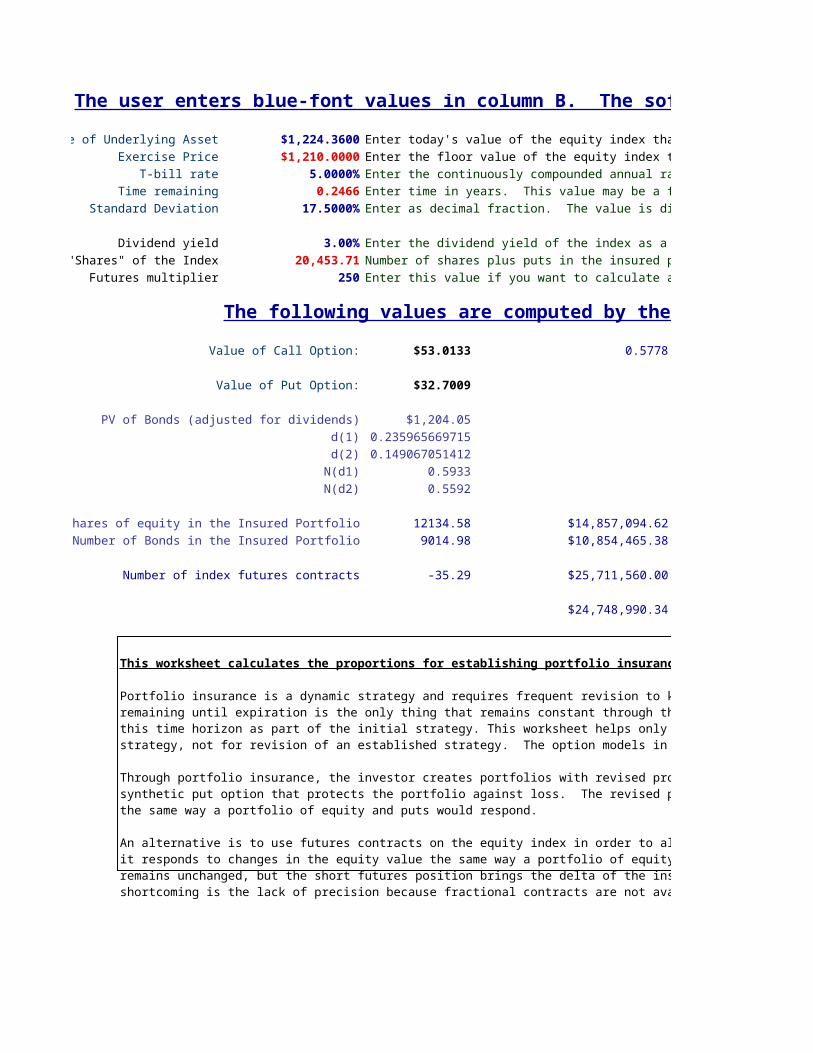
The user enters blue-font values in column B. The software transfers red-font data from the previous worksheet.
Value of Underlying Asset $1,224.3600 Enter today's value of the equity index that best fits the portfolio you wish to insureExercise Price $1,210.0000 Enter the floor value of the equity index that you wish to set as the insured level
T-bill rate 5.0000% Enter the continuously compounded annual rate as a decimal fraction. The value is displayed as a percentage.Time remaining 0.2466 Enter time in years. This value may be a fraction, such as 30/365 (type the following: =30/365).
Standard Deviation 17.5000% Enter as decimal fraction. The value is displayed as a percentage.
Dividend yield 3.00% Enter the dividend yield of the index as a decimal fraction"Shares" of the Index 20,453.71 Number of shares plus puts in the insured portfolio
Futures multiplier 250 Enter this value if you want to calculate a portfolio insurance strategy using futures contracts on the equity index
The following values are computed by the worksheet:
Value of Call Option: $53.0133 0.5778
Value of Put Option: $32.7009
PV of Bonds (adjusted for dividends) $1,204.05d(1) 0.2359656697152d(2) 0.1490670514119
N(d1) 0.5933N(d2) 0.5592
Shares of equity in the Insured Portfolio 12134.58 $14,857,094.62Number of Bonds in the Insured Portfolio 9014.98 $10,854,465.38
Number of index futures contracts -35.29 $25,711,560.00
$24,748,990.34
This worksheet calculates the proportions for establishing portfolio insurance strategies
Portfolio insurance is a dynamic strategy and requires frequent revision to keep up with changing equity values. The time remaining until expiration is the only thing that remains constant through the life of the insurance coverage. You choose this time horizon as part of the initial strategy. This worksheet helps only for the initial setup of the portfolio insurance strategy, not for revision of an established strategy. The option models in this worksheet are adjusted for dividends.
Through portfolio insurance, the investor creates portfolios with revised proportions of equity and bonds, creating a synthetic put option that protects the portfolio against loss. The revised portfolio responds to changes in the equity value the same way a portfolio of equity and puts would respond.
An alternative is to use futures contracts on the equity index in order to alter the response of the insured portfolio so that it responds to changes in the equity value the same way a portfolio of equity and puts would respond. The equity position remains unchanged, but the short futures position brings the delta of the insured portfolio toward the target level. The shortcoming is the lack of precision because fractional contracts are not available.

The user enters blue-font values in column B. The software transfers red-font data from the previous worksheet.
Enter today's value of the equity index that best fits the portfolio you wish to insureEnter the floor value of the equity index that you wish to set as the insured levelEnter the continuously compounded annual rate as a decimal fraction. The value is displayed as a percentage.Enter time in years. This value may be a fraction, such as 30/365 (type the following: =30/365).Enter as decimal fraction. The value is displayed as a percentage.
Enter the dividend yield of the index as a decimal fraction
Enter this value if you want to calculate a portfolio insurance strategy using futures contracts on the equity index
Delta of the insured portfolio
Amount held in equityAmount held in bonds
Total value of portfolio today
Floor value of insured portfolio
158%
242%
Proportions
This worksheet calculates the proportions for establishing portfolio insurance strategies
Portfolio insurance is a dynamic strategy and requires frequent revision to keep up with changing equity values. The time remaining until expiration is the only thing that remains constant through the life of the insurance coverage. You choose this time horizon as part of the initial strategy. This worksheet helps only for the initial setup of the portfolio insurance strategy, not for revision of an established strategy. The option models in this worksheet are adjusted for dividends.
Through portfolio insurance, the investor creates portfolios with revised proportions of equity and bonds, creating a synthetic put option that protects the portfolio against loss. The revised portfolio responds to changes in the equity value the same way a portfolio of equity and puts would respond.
An alternative is to use futures contracts on the equity index in order to alter the response of the insured portfolio so that it responds to changes in the equity value the same way a portfolio of equity and puts would respond. The equity position remains unchanged, but the short futures position brings the delta of the insured portfolio toward the target level. The shortcoming is the lack of precision because fractional contracts are not available.

158%
242%
Proportions
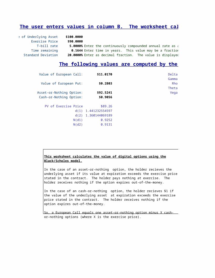
The user enters values in column B. The worksheet calculates the remaining values
Value of Underlying Asset $100.0000Exercise Price $90.0000
T-bill rate 5.0000% Enter the continuously compounded annual rate as a decimal fraction. The value is displayed as a percentage.Time remaining 0.1644 Enter time in years. This value may be a fraction, such as 30/365 (type the following: =30/365).
Standard Deviation 20.0000% Enter as decimal fraction. The value is displayed as a percentage.
The following values are computed by the worksheet:
Value of European Call: $11.0170 DeltaGamma
Value of European Put: $0.2803 RhoTheta
Asset-or-Nothing Option: $92.5241 VegaCash-or-Nothing Option: $0.9056
PV of Exercise Price $89.26d(1) 1.4412325545971d(2) 1.3601440691892
N(d1) 0.9252N(d2) 0.9131
This worksheet calculates the value of digital options using the Black/Scholes model.
In the case of an asset-or-nothing option, the holder recieves the underlying asset if its value at expiration exceeds the exercise price stated in the contract. The holder pays nothing at exercise. The holder receives nothing if the option expires out-of-the-money.
In the case of an cash-or-nothing option, the holder recieves $1 if the value of the underlying asset at expiration exceeds the exercise price stated in the contract. The holder receives nothing if the option expires out-of-the-money.
So, a European Call equals one asset-or-nothing option minus X cash-or-nothing options (where X is the exercise price).
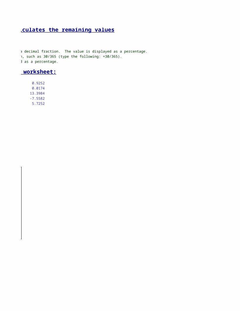
The user enters values in column B. The worksheet calculates the remaining values
Enter the continuously compounded annual rate as a decimal fraction. The value is displayed as a percentage.Enter time in years. This value may be a fraction, such as 30/365 (type the following: =30/365).Enter as decimal fraction. The value is displayed as a percentage.
0.92520.0174
13.3984-7.55825.7252
This worksheet calculates the value of digital options using the Black/Scholes model.
In the case of an asset-or-nothing option, the holder recieves the underlying asset if its value at expiration exceeds the exercise price stated in the contract. The holder pays nothing at exercise. The holder receives nothing if the option expires out-of-the-money.
In the case of an cash-or-nothing option, the holder recieves $1 if the value of the underlying asset at expiration exceeds the exercise price stated in the contract. The holder receives nothing if the option expires out-of-the-money.
So, a European Call equals one asset-or-nothing option minus X cash-or-nothing options (where X is the exercise price).