Optimum Structural Strength of Materials Flexible Pavements N. K. VASWANI, Virginia Highway Research Council, Charlottesville

• Ill

The optimum structural strength contributed by a material to the overall strength of the pavement was studied for cases applicable to Virginia. The variables were (a) the modulus of elasticity or the thickness equivalency of the material, (b) the thickness of the material in the layer, (c) the loca­tion of the material with respect to other layers containing stronger or weaker materials and in varying thicknesses, and (d) the effect of the total pavement thickness and the depth of the material from the top of the pave­ment. The investigation consisted of a study of the thickness equivalencies of the materials on Interstate, primary, secondary, and subdivision roads in Virginia, and a model study. The evaluation of the highway system was quantitative, while that of the model study was qualitative only. The investi­gation showed that the structural strength of a pavement is decreased when a weaker layer is placed over a stronger layer or when a weaker layer is sandwiched between 2 strong layers. The investigation also showed that, when the bottom of the top layer does not bend, the stress distribution is bulb type and that, when the bottom bends, the stress distribution is fan type. Each case would therefore need a different mathematical treatment for design.

•FLEXIBLE PAVEMENT DESIGN has undergone a change, in Virginia and other states, from the basic principle of designing each successive layer stronger than the layer underneath it. Materials having a high modulus of strength, e.g., soil cement, soil lime, and cement-treated aggregate, are now commonly used. These materials are placed in subgrades or bases and at various depths and positions in relation to other layers having a low modulus of elasticity. Because of this, the structural strength contributed by a given material is affected by the arrangement of the other materials in relation to the material under consideration.

In this investigation, the manner and the degree of strength contributed by a material in such pavement systems, with respect to the strength of other materials, have been studied. Two types of studies were made:

1. Determinations of the optimum thickness equivalency values of the materials used on primary, Interstate, secondary, and subdivision roads in Virginia, where the ihfok:-_ ness equivalency values are based on the location of the materials in the structure of the flexible pavement; and

2, Qualitative evaluation of the effect of thickness and modulus of strength of a given layer with respect to the thickness and modulus of strength of the other layers in the pavement system.

The thickness equivalency values of the materials with respect to their location in the structure were determined. The effect of the location of a given material in a pave­ment with respect to the other materials in the pavement system was determined, along with stress distribution patterns,

Paper sponsored by Committee on Flexible Pavement Design and presented at the 49th Annual Meeting.

77

78

PURPOSE

The main purpose oi this study was to determine the structurai behavior anci the op­timum use of a given material in a layered pavement system. It was proposed to de­termine the behavior and strength of the given material with respect to the modulus of strength and thickness of other layers in the system.

THICKNESS EQUIVALENCY VALUES OF PAVEMENTS IN VIRGINIA

The thickness equivalency value, a, is an index of the load-carrying capacity of a material and could be defined as the ratio of the strength of a 1-in. thickness of the material to that of 1 in. of asphaltic concrete or any other specified material.

In Virginia, different design standards are established for (a) primary and Interstate roads and (b) secondary and subdivision roads. In the case of primary and Interstate roads, the design is based on the subgrade CBR value and on traffic in terms of 18-kip equivalents. In the case of secondary and subdivision roads, the design is based mostly on traffic in terms of vehicles per day. The evaluations of thickness equivalency values for these roads were carried out as discussed in the following sections.

Primary and Interstate Roads

The evaluation of thickness equivalency values for primary and Interstate roads was based on (a) adoption of soil support values (based on CBR and soil resiliency), which would account for the regional factor; (b) traffic in terms of 18-kip equivalents; and (c) deflections. The thickness equivalency values have been reported previously (1, 2). These values were determined by multiple regression analysis. - -

A study of cement-treated aggregate subbases was carried out in this investigation and their thickness equivalency values, along with all the others previously determined, are given in Table 1.

Serial Number

J 2

3

TABLE 1

THICKNESS EQUIVALENCY VALUES OF MATERIALS IN FLEXIBLE PAVEMENT SYSTEM

Location

Surface Base

Subbase

Material

Asphaltic concrete Asphaltic concrete Cement-treated aggregate

over dense-graded ag-gregate base or soil ce-ment or soil lime and under asphaltic concrete mat.

Dense-graded aggregate, crushed or uncrushed

Select material I (Va. specifications) directly under asphaltic concrete mat . and over a subbase of a good quality

Select material cement-treated

Select material I, II, and III (Va. specifications)

1n Piedmont area In valley and ridge area

and coastal plain Soil cement Soil lime Select material cement-

treated Cement-treated aggregate

directly over subgrade

Values

Primary Secondary and and

lnterstate Subdivision Roads Roads

1.0 1.0 1.0 1.0

1.0 1.0

0.35 0.60

0.35

0 .80

0.0 0.0

0.2 0.50 0.4 0.60 0,4 0.55

0.4 0.80

0.6

79

Secondary and Subdivision Roads

The evaluation of the thickness equivalency values for secondary and subdivision roads was based mainly on traffic in terms of vehicles per day. The values determined by regression analysis were based on the present design practice in Virginia (3) by correlating daily traffic with the thickness index D = a1h1 + a2h2 + , .. in the equation log D = P + Q log vpd, where D = thickness index = a1h1 + a2h2 + ... ; vpd = number of vehiclesperday; h1, h2,, .. = thickness in inches of different layers; a 1 , a2, •• , = thick­ness equivalency of the materials with thicknesses h1, h2, ... respectively and a1 = l; and P and Q = constants of the equation. The following equation was obtained from 12 mean values:

log D = 0.2 + 0.24 log vpd

The correlation coefficient was found to be 0, 99, and the standard error of estimate was 0. 02. These values indicated a very high degree of correlation.

Effect of Depth of Cover and Pavement Thickness on Thickness Eguivalency Values

The primary and Interstate roads in Virginia usually carry high volumes of traffic while the secondary and subdivision roads carry comparatively low volumes. The pri­mary and Interstate roads are therefore stronger and thicker than the secondary and subdivision roads.

Examination of the thickness equivalency values given in Table 1 for the 2 sets of design procedures reveals the following:

1. The thickness equivalency of untreated aggregate in the base is 0. 35 for primary and Interstate roads, and 0. 60 for secondary and subdivision roads.

2. Similarly, the thickness equivalency values of the materials in the subbase for primary and Interstate roads are lower than the values for secondary and subdivision roads.

3. In the case of primary and Interstate roads, the thickness equivalency for the cement-treated aggregate is 1. 0 for the base course and 0. 6 for the subbase course.

The reason for these differences in the thickness equivalency values is the depth of the cover. In the case of primary and Interstate roads, the surfacing, binder, and base courses over the untreated aggregate would consist of asphaltic concrete varying in thickness from 4. 5 to 10. 5 in. Furthermore, an intermediate layer of about 6 in. of cement-treated aggregate is sometimes provided between the untreated aggregate base and the asphaltic concrete mat, which further increases the cover thickness. As com -pared to this thickness of cover, the cover thickness of asphaltic concrete over the un­treated aggregate base for secondary and subdivision roads varies from O to 5 in. The reduction in thickness equivalency with an increase in cover thickness has also been pointed out by Foster (4).

In some cases it has also been found that as the thickness of the pavement decreases the thickness equivalencies of the materials increase. This is evident from the data given in Table 1, wherein the thickness equivalency values of the subbase materials in secondary and subdivision roads are higher than those of similar materials in primary and Interstate roads.

Figure 1 has been drawn on the bases of the AASHO Road Test results (3 ). Figure 1 shows that, as the depth of the pavement increases, the thickness index required de­creases. For example, with 200,000 repetitions of the 20-kip axle load shown in Fig­ure 1, the thickness index decreases from 3. 31 to 3.14 when the pavement depth in­creases from 17. 4 to 23. 8 in.

In spite of the effect of the depth of cover and pavement thickness on the thickness equivalencies of t he materials, it is found that the equation of thickness index, D = a1h1 + a2h2 + , .. , holds. This equation is applicable if the thickness equivalencies of the ma -terials are determined according to their quality or strength and their location in the pave­ment system. However, during study of the flexible pavements in Virginia, certain ob­servations were made that, because of lack of data, could not be clarified. Therefore,

80

22 r----,----"""T---- ,------r----...,.-----, o ., ~"a Variable bases

,,, ~, r-1; 7 (Surfacing 311 .and Auhha.AA '1 11 )

~. '\/ !- I I

'b<P ;. o Crushed stone base. t-----i-----,.----- -;--........-- .<1-t---- XBituminous treated base . 20

\ ~ 0 0

"' 0

.2l 18 0 0 0

.s <'

.9 ... ?I. "' "C

.; 16

"' a "' 1. p.,

14

10 .__ ___ ....._ ___ ....... _ ___ ,__ ___ ....._ ___ ...... ~~~---

3.0 3. 2 3. 4 3.6 3. 8 4 . 0 4 . 2

AASHO Thickness index

Figure 1. Thickness index versus pavement depth (~. Fig. 36) .

model studies were conducted to investigate these observations. This study is discussed in the following paragraphs.

MODEL STUDIES

The study of pavements in Virginia indicated that, when the organization of the layered system deviated from that of the usual system, there was a change in the load-thickness in­dex relationship. It was not possible to make any theoretical verification of this fact beyond certain limits. [ Theoretical evaluations made on pavements in Virginia have been reported elsewhere (~). J The method of verification by models was therefore used. The object of the model studies was to obtain a qualitative evaluation of the be­havior of the pavement. No quantitative or numerical evaluation was proposed or should be assumed, although numerical values are given for clarity,

In all the studies mentioned here, the models consisted of 2, 3, or 4 layers of ma­terials arranged in varied order and in varied depths. The lowest layer consisted of a specified material-called the subgrade-having a modulus of elasticity= 1,000 psi for an infinite depth. The infinite depth of the subgrade was obtained by increasing the thickness of the subgrade layer until the load deflection ratio on the subgrade only re­mained almost constant. Some of the different combinations adopted are described later. All materials in the models were homogeneous, isotropic, and elastic within the testing range of load and time. All models whose results are reported were 2 dimen­sional on a 3-dimensional subgrade. The models were of a specified width to permit proper distribution of the load. The thickness of each layer was varied. The load was applied in the center of the model and maximum deflections were measured. The load­ing system on the 2- and 3-dimensional models is shown in Figures 2 and 3.

Figure 2. Loading system for 2· dimensional model.

Two Layers-Single Layer Over the Subgrade

Figure 3. Loading system for 3-dimensional model.

81

In a 2-layer system, the modulus of elasticity of the top layer is always higher than that of its subgrade, e.g., an untreated stone or soil cement, asphaltic mat, and so forth, over a weaker soil subgrade.

In this investigation, 3 photoelastic materials having moduli of elasticity values E = 30,000, 340,000, and 450,000 psi were independently loaded while resting on a weaker subgrade having an E = 1,000 psi. A graph of load versus deflection was drawn for each of the materials with different thicknesses of the top layer resting on the given sub­grade. All these curves were straight lines passing through the origin. The slopes of the curves differed from one another depending on the modulus of elasticity and the thickness of the top layer. From each of the graphs, deflection per unit load was de­termined. Based on the data so obtained, a curve of deflection per unit load versus thickness of the top layer was drawn for each of the materials with a given modulus of elasticity. (Deflection per unit load was adopted to enable evaluation for any given load.) Three such curves, one each for E = 30,000, 340,000, and 450,000 psi of the top layer, are shown in Figure 4.

To correlate the thickness equivalency of each of these 3 materials, the thickness equivalency of the material with E = 340,000 psi was taken as a 1 = 1. 0. For different values of deflection, ratios of the thickness of the layer of material with E = 30,000 psi to the thickness of the material with E = 340,000 psi were determined from Figure 4. There was very little difference between these ratios. The general trend was a slight decrease in the values of the ratios with an increase in the thickness of the layer or a decrease in deflection. An average value of this ratio was found to be 0.27. Thus, this ratio is the thickness equivalency value, as, of the material having Es = 30,000 psi. In the same manner, the thickness equivalency value of the material having E2 = 450,000 psi

82

8. 0

7 . 0

I -• . iv -!~arilble a or .t... var 1an1e

6. 5

6. 0

5. 5

- ~ E = 11 000 psi -~ \ '

5. 0

4. 5

4. 0

"' 3. 5 ~ j

3. 0 ~ a .§

2. 8

z 2. 6 ~ ~ 2. 4

"' 2. 2

2. 0

l. 8

l. 6

\.

"~ ~ "' e

!',._.J ".Jo

\\ " • 0110

~""1,. r---...._ ~"

\\ ~?

[\ ~ ... .. ,_

' ' ....

' ' '\ " e ./'"

~ "-... .2.,()

~ ~ "' N:' II

'01)0

--......:..."";, -........ ............... ... ·i .. , "'~·?,;

.......... ..... _ l, 4

l, 2

l. 0 0 O.l 0.2 0.3 0, 4 0.5 0.6 0.7 0.8 0.9 l , O I.I 12

h = thickness in inches

Figure 4. Deflection versus thickness (2-layer system).

was fowid to be a2 = 1. 40. The thickness equivalency value of the material with E2 = 450,000 psi decreased very little with an increase in the thickness of the layer, as was observed for the material with Es = 30,000 psi, and hence this difference is ignored and the average value accepted. Thus, the following values for different materials were accepted for further tests:

1, For E1 = 340,000 psi, a1 is 1.0; 2. For E2 = 450,000 psi, a2 is 1.4; 3. For Es= 30,000 psi, as is 0.27; and 4. For E4 = 1,000 psi, ~ was not determined, because the E value of the subgrade

was also 1,000 psi.

Three Layers-Two Layers Over a Subgrade

In the 3-layer system either the top layer could be stronger than the bottom layer (e.g., an asphaltic concrete mat lying over an untreated stone l>ase), or the top layer could be weaker than the bottom layer (e.g., stone aggregate lying over a cement-treated

83

subbase or an asphaltic mat lying over a portland cement concrete pavement). The model tests showed that, when a stronger layer lies over a weaker layer, the equation of log d = M + N (a1h1 + a2h2 + ..• ), which is based on the AASHO Road Test results and was adopted for the work reported elsewhere (5), is applicable with d = deflection, M and N = constants of the equation, and a1, a2, h;, and h2 having the same meaning as de­scribed previously.

In Figure 5, thickness index versus deflection has been drawn for the 3-layer sys­tem and the 2-layer system. The values of the 3-layer system were obtained directly from load tests, while the values of the 2-layer system were obtained from the curves shown in Figure 4, which were drawn from the load test data. Excluding the very low values of thickness index, say up to a maximum of D = 2, the graph of deflection, d, versus thickness index, D, would be a straight line. Lower values of D are ignored be­cause pavement designs with such low values would be impractical. However, the straight-line graph shown in Figure 5 is based on a simple regression analysis of all points shown in the graph. A high degree of correlation (R = -0. 97) exists between these 2 variables-deflection and thickness. · With a1 = 1.0 for the upper layer, as determined from the 2-layer system discussed

in the preceding, it was found that the thickness equivalency of the lower layer with a lower strength modulus increases as its thickness decreases, as shown in Figure 6. The increase is from a value of 0.27 as determined in the 2-layer system to 0.48 for the minimum thickness adopted. This tendency has been observed in pavements in Virginia. H.B. Seed et al. (6) have shown thatresilientdeformationperinchofgranular base is smaller for an 8-in. base than for a 12-in. base. Resilient deformation is an inverse function of the thickness index, and hence an inverse function of the thickness equivalency. Thus, the investigation by Seed et al. also shows that the thickness equiv­alency of the lower layer increases as its thickness decreases. It could be concluded, therefore, that the optimum thickness value for the lower layer is the minimum thick­ness that could be economically provided.

6

:e 0

5 N talion~ :

... (l)

0

"' 0 ~ 4t-~~~-t-~--t-~--+~~+-~+­o 0 0

0 g 3 t-~+------""'f,,,;;::-<'-t-~---1~~+-~+-

] j

Case 2 - (two layers)

~ n or E V"rlnb l.e l" h variable

~ -..:;~"""'""""""""' N. E = 1, 000 psi. ,

o E3

= 30,000

x £ 1 = 340, OO(l

01· a.3

"' 0. 27 (two laye1·J

o\; ~ -= l. 0 {lwo layer)

• E 2 = 450, 000 or n2 = l. •10 (lw-0 layer)

6 h1 -== 0.125" Md h3

variable (lhree laJers)

"' h1. = 0. 25" and h3 varlnble (th1·ea lnyers)

• \ = 0. 5" and h3 variable (,three la erij)

& 2t-~+-~-t-~-t-~---1~~r-11 ....... +:---c,..:::,,,'*,-~-t-~--+~~1--~+-~--+-~-+~---I

~ " (l)

,;:::

~

0

Equation log d = 1. 644 - 3. 047 D Correlation coefficient = -0. 97 Standard error of estimate = . 03

2 3 4 5 6 7

D = Thickness index

9 10 11

Figure 5. Deflection versus thickness index (model study).

12 13 14

84

II

.r'

1. 5

0.5

o.o 0. 1

E1 .. 3-10 ,000;,si.n 1

• 1. O E "30 ,OOOpsl. n:i "0. 27 ~,,-.?,,,,,,,,,,,,, ,,-..: ;,_'\;"

E = 1,000 psi

h1 0. 5"

0. 2 0.3 0. 4

h3 = Thicknes s of lower l ayer, E3

= 30, 000 psi.

Figure 6. Weaker layer underneath a stronger layer.

o. 5 0 . 6

In the model study, when a stronger layer was laid under a weaker layer, as shown in Figure 7, the model did not exactly fit the equation log d = M + N (aib.1 + a2h2 + ... ) as it offered less resistance to deflection. Assuming that a2 = 0. 27 for the upper layer as determined from the 2-layer system discussed previously, it was found that as the thick­ness of the top layer increases, the thickness equivalency contributed by the lower layer decreases. This is shown in Figure 7. The reduction in the value of the thickness equivalency of the lower layer depends on the ratio of the modulus of the 2 layers and also on their thicknesses. Figure 7 also shows that the thickness equivalency of the lower layer increases as its thickness increases.

Figure 7 thus shows that the strength equivalency value, a1, of the stronger lower layer decreases from 1. 0 to 0. 6, which is dependent on layer thickness if a2 is taken as 0.27. Thus, the materials in this system remain below their optimum strengths.

Four Layers-Three Layers Over a Subgrade

In this system, if the modulus of elasticity decreased from top to bottom, no change was noticed from the fundamentals discussed in the 3-layered system with the stronger layer over the weaker layer, i.e., log d = a + b (a1h1 + a2h2 + ••• ).

a, . ..: £ [ ..... 0 0 0 ;,.,o. 1.0 c.> 0 = ... .s "' oS II

-~ ~ C' • "' .. : ~ 0. 5

!-;:: c.>"'

~] II

0

E = 1,000 psi

I -h3 = 0.125"-

113 ~ o. 25",..,...-

h3 = 0.5"-_.............

.-,--

0. 1 0. 2 0.3 0. 4 0.5 0.6

h1

= Thiclmess of lower layer in inches, E1

= 340,000.

Figure 7. Stronger layer underneath a weaker layer.

85

The system discussed here, and which sometimes is found in practice, is the case when a weak layer is sandwiched between 2 strong layers. Two systems of sandwiched layers are discussed. In one case, the sandwiched layer had an E4 = 1,000 psi with the sandwiching layers having an E1 = 340,000 psi as shown in Figure 8. In the other case, the sandwiched layer had an E3 = 30,000 psi with the sandwiching layers having an E1 = 340,000 psi or 450,000 psi. The case of the sandwiched layer with an E3 = 30,000 psi and sandwiching layers with an E1 = 340,000 psi is shown in Figure 9.

In both cases the model did not exactly correspond to the equation log d = M + N (a1h1 + a2h2 + ••• ) and the following was observed:

1. Assuming that the normal thickness equivalency value is a1 = 1. 0 for the sand­wiching layers with an E = 340,000 psi, the strength contributed by the weaker sand­wiched layer (i.e., the value.s of a2 or a3 ) decreased with an increase in thickness of the sandwiching layers (Figs. 8 and 9).

2. By decreasing the modulus of elasticity of a sandwiched layer, tpe strength con­tributed by the sandwiched layer decreases considerably as compared to its normal strength and is even sometimes negative (Figs. 8. and 9).

The negative thickness equivalency value shows that the pavements are not rein­forced by the sandwiched layer, but that, on the contrary, their total strength is de­creased This same behavior was observed on an experimental project in Virginia where a select soil material was sandwiched between soil cement underneath it and stone base or cement-treated aggregate and asphaltic concrete over it. The deflec­tions as related to supposedly comparable projects were higher, and it is believed that, if this layer had not been introduced, the deflections of the pavement would have been lower. In other words, the thickness equivalency of this sandwiched material was nega­tive, with a higher deflection thus being obtained.

This negative thickness equivalency value could be explained by the observationmade on the stress distribution for weak sandwich layers. In these layers the angle of the spread of the load increases with a decrease in the modulus of elasticity of the sand­wiched material. It is obvious, therefore, that the introduction of a weaker sandwiched layer provides 2 effects: (a) It spreads the load, over a larger area and thus transmits very little load intensity to the underlying layer; and (b) the variation in thickness of the

(ll

C.

h4 = Thickness of sandwiched layer in inches, E4 = 1,000 psi

o. 1 0, 2 0.3 0. 4 0,5 o o~---~---~---~---~---~~----, 0 0

...; II

iii

Figure 8. Weaker layer ( E = 1,000 psi) sandwiched between two stronger layers.

86

"' "" 0 0 0

g o. 5 t-----i-----i----=::t-

11

"' "'

0 t------::t-:----O::t-:,2---,:10 -::3----;:'0t-,4,-----+-. ""5 -----,O:f-6::-. ----1

h3

= Thickness of sandwiched layer , E = 30, 000 psi

-1.5 t----t----:,---t-----+-----+-----+-- ---+-----I

-2. 0 ----~---..._ ___ ..._ ___ _._ ___ _._ ___ _._ ___ __,

Figure 9 . Weaker layer (E3

= 30,000 psi) sandwiched between two stronger layers.

sandwiched layer does not seem to affect the system much, as long as the sandwich layer remains in compression only,

Use could be made of these 2 effects in the optimum design of pavements. For ex­ample, when the subgrade is weak or resilient, a sandwich layer system could be utilized to spread the load over a larger area. Because the load intensity transmitted to the underlying layer is small, the choice of material and thickness design of the underlying layer could be such as to provide more rigidity than strength. Further, the thickness of the sandwich layer need not be increased beyond a certain minimum.

The reduction in the overall structural strength of this type of sandwich system does not eliminate its use. There are cases in which this flexible sandwich layer helps in other respects, e.g., by preventing reflection cracks in the bottom sandwiching layer from traveling into the top sandwiching layer.

Stress Distribution in Layered Systems

By means of a polariscope, the stress distributions in layered systems were de­termined. They were mainly of 2 types: (a) the bulb type, as shown in Figure 10; and (b) the fan type, as shown in Figure 11.

Bulb-Type Distribution-The bulb-type distribution was found in the following cases. The amount of stress and the degree of distribution depended on the thickness and the modulus of elasticity of the materials in the layered system.

1. Two-layer system-The underlying layer was a subgrade of infinite depth having an E = 30 x 106 psi. The overlying layer consisted of varying depths of 0. 5 in. and above, and the modulus of elasticity was equal to 1,000, 30,000, 340,000, or 450,000 psi.

---~= 1,000 P.S I

-E=l,OOOJ>S I.

Figure 10. Stress distribution when a weaker layer lies over a stronger layer.

--- E2:450,000 P.S.I.

--E=l,000 P.S.I.

Figure 11. Stress distribution when a stronger layer lies over a weaker layer.

87

2. Three-layer system-The underlying layer was of infinite depth having an E = 1,000 psi. The overlying 2 layers consisted of the top layer of thickness 0. 5 in. or more and an E = 1,000 or 30,000 psi. The layer below the top layer had a thickness of 0.5 in. or more and and E = 340,000 or 450,000 psi, i.e., a modulus of elasticity much higher than that of the material above it. An example of this is shown in Figure 10. The bulb­type distribution is clearly defined in the topmost layer only when the underlying layer or the layered system is very rigid.

From this it is evident that when a weaker layer, such as untreated aggregate or a combination of thin asphaltic concrete over untreated aggregate, lies over a stronger layer, such as a good quality soil cement or cement-treated aggregate, the stress dis­tribution will be bulb type. In other words, it may be stated that, when the lower layer prevents bending of the bottom side of the top layer, the stress distribution will be of the bulb type, and Boussinesq' s theory, or theories based on Bo us sine sq' s evaluation, could be applied.

Fan-Type Distribution-The fan-type stress pattern was found in the following cases. The amount of stress and the degree of distribution depended on the thickness and the modulus of elasticity of the materials in the layered system.

1. Two-layer system-The underlying layer was a subgrade of infinite depth having an E = 1,000 psi. The overlying layer consisted of varying depths and had an E = 1,000, 30,000, 340,000, or 450,000 psi.

2. Three-layer system-Various combinations in thicknesses of 2 layers over asub­grade material of infinite depth with an E = 1,000 psi were found to give a fan-type dis­tribution in the top layer. These combinations were as follows: The lower layer had an E = 30,000 psi, and the upper layer had an E = 340,000 or 450,000 psi; or the lower

88

layer had an E = 340,000 psi, and the upper layer had an E = 450,000 psi. An exampie of this is shown in Figure 11.

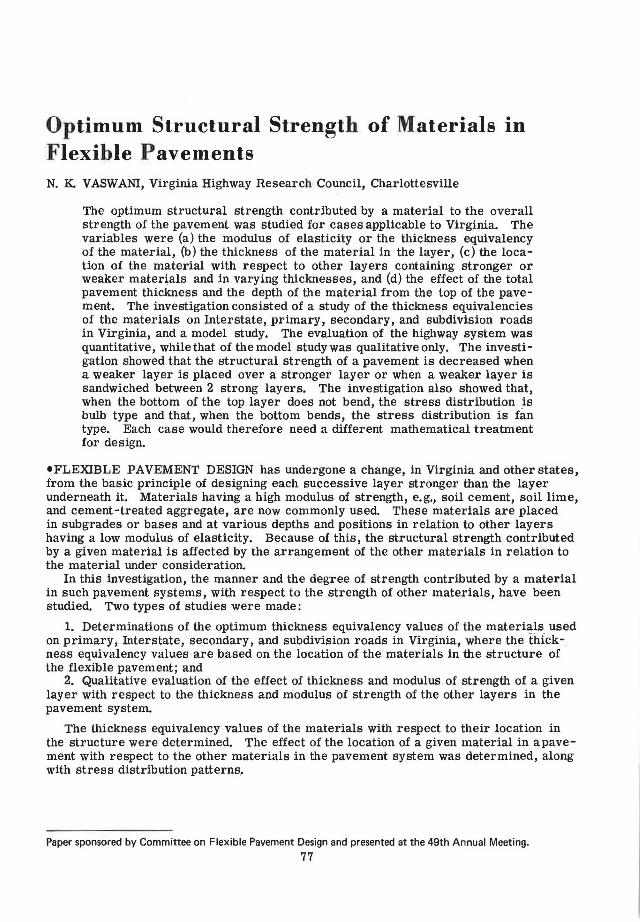
3. Four-layer system-In all the sys­tems tried, the sandwiched layer was weaker than that of the other 2 layers. In almost all cases a fan-type distri­bution was observed in the top layer. In a few cases, when the ratio of the modulus of the sandwiching layers and the sandwiched layer was low and the thickness of the sandwiched layer was also low, a combination of bulb- and fan-type stress distribution was ob-served.

---E1= 340,000 P.S .I,

E1= 340,000 P.S.I

- E=l,OOOP.S.I.

Figure 12. Effect of joint between two layers (in this case of the same modulus).

From the preceding observations, it could be concluded that, when the layer under­lying the top layer has a low modulus of elasticity and the overlying layer has the same or a higher modulus of elasticity, fan-type distribution takes place in the top layer. In other words, it may be stated that, when the bottom side of the top layer bends, the stress distribution will be fan type and the design of the top layer should be based on the avoid­ance of failure along the shear plane as recommended by McLeod (7) and by others.

Effect of Deep Strength-The stress distribution pattern in 2 layers of the same mod­ulus and varying depths lying over a subgrade layer was carried out with partial bond between the 2 layers that could slide over their contact surface after a certain amount of load was applied. The pattern of stress distribution in the top and lower layers was always of the form shown in Figure 12. This shows that when a certain depth of a spec­ified material is laid in more than 1 layer and there is no perfect bond between the 2 layers the structural behavior is different as compared to that of 1 deep layer. The difference in the strength contributed depends on the thickness of the 2 layers and the

- E1=3 .. 0 ,000 P.S.I.

. ' ·"':i"' ~i-'a~' -E4

= 1,000 P.5.1. =-----,:::;

-E1=340,000 P.S.I.

-E= 1,000 P. S .I.

(a)

(cl

1bl

E 1= 340,000 P.S . I.

--- E'\=30,000 P.S .I.

- E=l,000 P.S .I.

--E =1,000 P.S.I .

Figure 13. Weaker layer sandwiched between two strong layers (for sandwiched layer, E = 1,000 in a and b and E = 30,000 psi inc).

89

modulus of elasticity of the material in each. The overlying layer in combination with the underlying layer provides less structural strength than when laid in 1 depth.

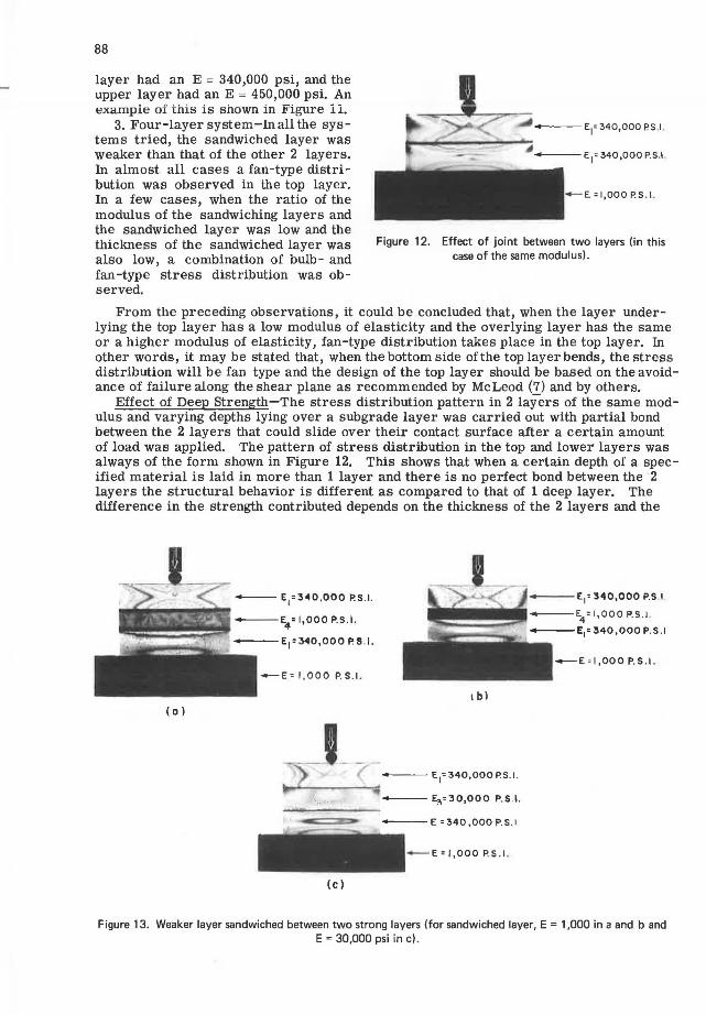
Effect of Weak Sandwiched Layers- Figure 13 shows the stress distribution for 3 cases of a 4-layered system. In Figures 13a and 13b, the s andwiched layer consists of material with an E = 1,000, but the thickness of the sandwiched layer in Figure 13b is half the thickness of the sandwiched layer in Figure 13a.

No stress lines are noticed in the sandwiched layers in Figures 13a and 13b; instead, 3 horizontal bands are noticed in Figure 13a. The 2 bands near the contact surfaces with the top and bottom layers were deep brown in color, whereas the central band was light brown. In the case of thinner sandwiched layers, as shown in Figure 13b, the color was uniformly deep brown. Both Figures 13a and 13b therefore indicate uniform stress of compression with higher stresses near the contact surface. This uniform stress of compression indicates an increase in the spread of the load over the top of the sand­wiched layer. Thus, it is concluded that the angle of spread of the load increases with a decrease in the modulus of elasticity of the material of the sandwiched layer.

Comparing Figures 13a and 13b, we find that under the same load there is no change in the stress distribution in the lower sandwiching layer, except in the sandwiched layer itself. This shows that the thickness of the sandwiched layer does not affect the sys­tem below the top sandwiching layer.

Figure 13c shows a sandwiched layer with a higher modulus of elasticity (30,000 psi) as compared to that shown in Figures 13a and 13b. Stress lines are visible in the sand­wiched layer, and the load transfer to its underlying layer is greater than for a weaker sandwiched layer. Thus it shows that, as the modulus of elasticity of the sandwiched layer decreases, the transfer of load through the lower sandwiching layers decreases.

CONCLUSIONS

1. Investigations of satellite pavements on primary and Interstate roads of Virginia and the secondary and subdivision road designs for Virginia, coupled with model studies, have shown the following:

a. The strength contributed by a pavement could be represented by a thickness index of D = a1h1 + a2h2 + . • . as given by the AASHO Road Test results. The thickness equiv­alency value of the material depends on its strength and location in the pavement system.

b. The thickness equivalency value of the material decreases as the thickness of the cover increases, and vice versa.

2. The following conclusions are drawn from the model studies:

a. In the case of a single layer resting on a subgrade, the thickness equivalency of the material in the layer decreases very little with an increase in depth, and hence this variation could be ignored.

b. In a 3-layer system, when a stronger layer lies over a weaker layer (e.g., an as­phaltic concrete mat over a stone base), the optimum thickness of the weaker layer is the minimum thickness one could provide economically.

c. In a 3-layer system, when a weaker layer lies over a stronger layer (e.g., untreated aggregate over treated aggregate) the structural strength of the pavement, or resistance to deflection, is less compared to when the layers are reversed.

d. When a weaker layer lies over a stronger layer and if this underlying strong layer prevents bending in the bottom side of the top layer, the stress distribution is bulb type. In such a case, Boussinesq's theory, or theories based on Boussinesq's evaluation, can be applied.

e. When a stronger layer lies over a weaker layer or over a layer of the same strength, the underlying layer permits bending in the bottom side of the top layer, and the stress distribution will be fan-type. In such a case the design of the upper layer should be based on the avoidance of failure along the shear plane.

f. In the case of a 4-layer system with a weaker material sandwiched between 2 layers of stronger materials, the strength contributed by the sandwiched layer decreases with an increase in the thickness of the sandwiching layers.

90

g. The strength contributed by the sandwiched layer decreases, and even becomes negative, with a decrease in its modulus of elasticity.

ACKNOWLEDGMENTS

The support of the Pavement Section of the Virginia Highway Research Council and J. H. Dillard, state highway research engineer, is gratefully acknowledged. Special thanks are given to F. C. McCormick, professor in the Department of Civil Engineering of the University of Virginia's School of Engineering and Applied Science, for allowing use of his laboratory facilities. The work was financed from highway planning and re­search funds.

REFERENCES

1. Vaswani, N. K. Design of Pavements Using Deflection Equations From AASHO Road Test Results. Highway Research Record 239, 1968, pp. 76-94.

2. Vaswani, N. K. Design of Flexible Pavements in Virginia Using AASHO Road Test Results. Highway Research Record 291, 1969, pp. 89-103.

3. The AASHO Road Test: Report 5-Pavement Research. HRB Spec. Rept. 61E, 1962. 4. Foster, C. R. Discussion on Nichol's paper on "A Practical Approach to Flexible

Pavement Design." Proc., Second Internat. Conf. on Struct. Des. of Flexible Pave­ments, 1967,p. 657.

5. Vaswani, N. K. AASHO Road Test Findings Applied to Flexible Pavements in Virginia-Final Report. Virginia Highway Research Council, Charlottesville.

6. Seed, H. B., Mitry, F. G., Monismith, C. L., and Chan, C. K. Prediction of Flexible Pavement Deflections From Laboratory Repeated-Load Tests. NCHRP Rept. 35, 1967.

7. McLeod, N. W. Some Basic Problems in Flexible-Pavement Design. HRB Proc., Vol. 32, 1953, pp. 90-118.

Discussion C. R. FOSTER, National Asphalt Pavement Association-The thickness equivalencies

that Vaswani gives in his paper for untreated base and for certain other materials are lower for heavy-duty roads (primary and Interstate) than for light-duty roads. He stated that the reason for the pattern is the depth of cover. For heavy-duty roads, the untreated base would be deeper in the section than on a light-duty road.

Vaswani offers 2 elements of data to support the use of lower equivalencies for the heavy-duty roads. One element of data is Figure 1 taken from Figure 3 6 of the AASHO Road Test (3) and is presented with the comment "as the depth of pavement increases, the thickness index required decreases." However, thickness index is not the same as thickness equivalency, so this plot does not support a decrease in thickness equivalency with an increase in depth of cover.

Vaswani's other element of data is this statement: "The reduction in thickness equivalency with an increase in depth of cover thickness has also been pointed out by Foster." Although this appears to lend support, it really does not because we used dif­ferent thickness equivalencies. Vaswani assigned unity to asphaltic concrete, whereas I assigned unity to the untreated base. My values are the reciprocal of his. If I con­vert my statement to the thickness equivalency as defined by him, it would have to read "an increase in thickness equivalency with an increase in depth of cover."

Figure 14 shows a plot of the data of the average thickness equivalency of the hot­mix asphalt base in the AASHO Road Test versus thickness of hot-mix asphalt base that I prepared from AASHO Road Test data (3 ). The 5 points for each load represent thicknesses of untreated base divided by thickness of asphalt base at serviceability in­dexes of 1.5, 2.0, 2.5, 3.0, and 3.5 after 1,114,000 repetitions plotted against the thick­ness of the hot-mix asphalt base. Adjustments were made for variations in surface

,.. u z

4

~ 3 s s (/) (/) w z "' <,! I .... w 2 ~ a: w ;ix

. 12

', ·~ ~~. ... ?4

',• ~ .......... ~,'J~

I~

- · SINGLE AXLE

a TANDEM AXLE

NUMBERS DESIGNATE AXLE LOAD IN IOOO LBS

I

DATA FROM FIGURES 32 TO 34 OF

AASHO ROAD TEST REPORT 5

........ ~ ... .... a-'.'.~.

22. Ill 48 -:

""'to-:-:;-.. 30 --~ 9-- ... --: ~-r--

I 2 3 4 s 6 1 e !1 10 H

THICKNESS OF HOT MI X ASPHALT BASE- INCHES

Figure 14. Average thickness equivalency versus thickness of hot-mix asphalt base.

91

12

and subbase thicknesses by using the procedures described in the report. Wheel loads not tested were interpolated.

Without question, the thickness equivalency (as I define it) in the AASHO Road Test decreased with increase in thickness of hot-mix asphalt base. A review of the varia­tion in strength with depth in base course materials offers a reasonable explanation of the pattern shown in the AASHO Road Test.

At this point we need to define what we mean when we say strength. Strength is commonly used in reference to a breaking value such as in concrete. However, we are not concerned with this type of strength. What we are concerned with is the ability of the base course to develop strength under loading. An untreated base course will have a very small residual capacity to resist load because of tension in moisture films and surcharge of the overlying pavement, but the majority of the resistance to load is developed from the load being applied. Ability to develop strength under load is rated by the modulus of elasticity. Because the strains in the pavement are low, gen­erally well under 1 percent, we are concerned with the modulus at low strains. The modulus of untreated base courses at low strains is highly dependent on the degree of compaction. Test data plus my observations over the years show that it is impossible to obtain a high degree of compaction and a high modulus in the fir st few inches of un­treated base over the subgrade. Figure 15, from the Barksdale Field tests (_!!), shows a str ong tr end for the in-place CBR of the base material, both as constructed (indicated by tests outside the traffic lane) and after traffic, to increase with the height of the test above the subgr ade. Since pr eparing thi s plot, which incidentally was p r epared in 1943, I have observed this pattern in p1·actically all the other test pits or trenches that I have seen cut in pavements . This pattern was vividly brought out during studies (~)conducted at the Waterways Experiment Station in the mid-1950's to develop CBR design curves for metal landing mat. An equivalency concept was used in that a given design of metal mat was rated as the equivalent of a given thickness of crushed aggregate base. With this concept, the existing CBR design curves for flexible pavements could be used to produce curves for landing mats. (Incidentally, the concept worked well , but this i s not the point of discussion.) This equivalency concept was spot-checked by traffic test s. Test sections were built with mat placed on the s ubgrade and on 3, 6, and 12 in. of crushed aggregate base course. Although the base material was a dense-graded crushed

92

U)

"' r 4G u ~

~ : lO Cl m ::, U)

~ ~ 0 m < ~ w 10 1-... 0 I-r Cl iii r

0 0

U)

"' r u z ;;; 0 :

20

10

0 0

20,000 LB. TRACK

' t-- i..-..

_/v'f 1,-~ 10

SELECTED LOAM TESTS IN PLACE

40

10

u 0

S0,000 LB. TRACK

/ loo ' ~ . 00 'lfb ) ........... ,.

u ~ I I

10 20 30 Cl m ::, U)

CORRECTED C B R -1 SOAKED ST ANDA.RO CORRECTED C .8 .R -1 SOAKED STANDARD

"' PENETRATION SURCHARGE- WEIGHT OF PAVEMENT AND BASE

i5 m < 1-U)

~ 20 ... 0 I­r Cl 10 iii r

0 0

D ;,

• I /'

'f' " 10 20 30

CORRECTED C 8 R-1 SOAKED STANDARD

10

0 0

nl

I cio

• .

10 20 30 40 CORRECTED C 8 R -ll SOAKED STANDARD

ITEM !5, !50,000 LB, TRACK

-" . 0 n-

C . . --., 0 I

• • IOo I

lfb . ~ 0( ,i:, . • • • on,

4G 80 120 160

NO PENETRATION SURCHARGE

-

LIMESTONE BLEND TESTS IN PLACE

200

30

20

~ 71

10

0 0

..,,, 0

0

ITEM !5 .. 20 .. 000 LB, TRACK

,~. 0 no u . .

"" 0 0

-· 40 80 120 160

CORRECTED C .8 .R.-1 SOAKED STANDARD CORRECTED C ,8 R-1 SOAKED STANDARD

PENETRATION SURCHARGE-WEIGHT OF PAVEMENT AND BASE

LEGEND

-----INSIDE TRACKING LANE

0------0UTSIDE TRACKING LANE

NOTE: Points ere slngla tests,

Figure 15. CBR height of test above subgrade-selected loam and limestone blend.

200

limestone that had developed CBR values well above 80 in other tests where thick lifts were used, it was not possible to obtain a CBR of 80 in the 3-in. sections even though these were placed on a fairly strong subgrade (CBR 14) or even in the 6-in. sections placed on a weaker subgrade (CBR 5). Average CBR values are given in the following data:

Item

Low CBR subgrade Number of test sections Average CBR of subgrade Average CBR of base Average density of base Ratio CBR of base-subgrade

Medium CBR subgrade Number of test sections Average CBR of subgrade Average CBR of base Average density of base Ratio CBR of base-subgrade

3 in.

7 13.6 51

140.0 3.0

Crushed Aggregate Base

6 in.

24 4.9

50 144.8

10.2

15 11.2 93

146.5 8.3

12 in.

16 5.8

86 145.2

14.9

93

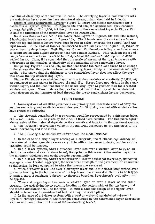
It should be noted that these averages represent a large number of tests. For ex­ample, a total of 24 test sections were built with 6 in. of base over the weaker sub grade. At least 3 CBR tests were made in each section. All values represent in-place tests on the as-constructed base course except for those in the 3-in, section. The as­constructed values for the 3-in. section showed wide variability. Those after a small amount of traffic (40 coverages) were much less variable, and these were used. These tests show that the in-place CBR of the base course was dependent on both the CBR of the subgrade and the thickness of the base. Apparently a large part of the variation is due to density, because there is a general trend for the CBR to increase with an increase in density. Figure 16 shows a plot of these CBR data with CBR plotted as a ratio of base CBR to subgrade CBR against base thickness. It is believed there are certain natural limits. First, if the subgrade is very strong, the ratio will probably approach 1. Also, regardless of the subgrade strength, the ratio would probably approach 1 at a base thickness slightly under 2 in., which is the diameter of the CBR piston. The data shown in Figure 16 indicate that the ratio increases slightly with a decrease in subgrade CBR and rapidly with an increase in base course thickness. Interpolated curves for subgrade CBR values of 5 and 10 are shown in Figure 16. Heukelom and this author (10) showed that in-place CBR values correlate fairly well with moduli measured in place with vibratory methods and suggested the conversion at 100 to 1 in metric units,

16 -.,"" o 5.B INTERPOLATED FOR SUBG RADE 'v"" CBR =5 _,, .,.

~ _, .,,.

u 12 .,, w .,, Q .,,. ~ 4. 9 9-"" "' "' ~ :::, FOR SUBGRADE V,

~ CSR = l 0

8 / a: / "' u / w b' ~ MEASURED SUBGRADE CBR "' ::::: 4 I "'" I.. ~ I, • 13.6

0 ,____. _ __._ _ _._ _ _.__ ..__--''---L---J..-...L..--'-- ..__---' 0 4 10 12

TH I CKNESS OF BASE - I NCH ES

Figure 16. Ratio of base and subgrade CBR versus base thickness.

94

200r 120

160

0 0

~ 100

" ~ 1 20

Bo V,

3 ~ 0 "' "' 0 '-' "' 60 w Bo V,

"' ~ 0 '-' w V, •D "" "' •D

20

0 ....___._ ...... _____ ...__.___. _ _.__ ........ _ _.__..___. 0

0 2 4 6 8 10 1 2

HEIGHT ABOVE SUBGRADE - INCHES

Figure 17. Base course modulus versus height above subgrade.

which is approximately 1,400 to 1 in English units. Applying this conversion factor (CBR x 1,400 = moduli in psi) to subgrades with CBR values of 5 and 10 and to the ratios shown in Figure 16 produces the variation in moduli with subgrade moduli and base course thickness shown in Figure 17. This plot shows that the base course modulus will increase rapidly with height above the subgrade, being quite low direcUy above the sub­grade and quite high when substantial thicknesses of base are used.

Treated base courses, such as hot-mix asphalt base and cement-treated bases, de­velop stiffness by cementation, and the moduli at low strains are not so dependent on compaction as untreated base courses. The modulus of a given hot- mix asphalt base will also vary according to rate of loading and temperature. Because we are concerned mainly with moving loads, rate of loading is not of primary concern except that persons running laboratory tests should use rates of loading comparable to those experienced on the road

The temperature within a hot-mix asphalt base course at any one time is a complex function of heat flowing in and heat flowing out. However, the average temperature (average for year) at the bottom of a thicker base would be a little lower than the aver­age for a thinner base. Thus, the modulus of a hot-mix asphalt base could be expected to increase a little with depth. For the purpose of this illustration, however, we will assume that the average modulus is constant with depth.

We have no in-place data on the modulus of hot-mix asphalt pavement, so we have to depend on laboratory tests and inference. Values reported in the literature range from 200,000 to 2,000,000 psi. The performance of hot-mix asphalt base under traffic implies, at least to me, a modulus in the range of 1,000,000 to 1,500,000 psi, and for the following illustration I have used a value of 1,250,000 psi.

The layered theory of pavement design presented by Burmister (11) in 1943 shows that the stress induced in a given subgrade under a given condition ofload is primarily a function of the thickness and moduli of elasticity of the overlying layers. A base with a high modulus of elasticity would transmit a lower stress to the subgrade than a low modulus base of equal thickness. To state this in another way, a given thickness of low modulus base would transmit the same stress to the subgrade as a lesser thickness of high modulus base. Thus, the ratio of the elastic modulus of one base course to the elastic modulus of another base course is a form of thickness equivalency.

The data shown in Figure 17 can be used to show that the ratio of the modulus of hot-mix asphalt base to the modulus of untreated base decreases with thickness of untreated base. For example, assume that a sub grade has a CBR of 5 and thicknesses of untreated base of 6 and 12 in. For the 6-in. base the modulus would be about 7,000 psi at the bottom and about 70,000 psi at the top for an average of 38,500. The hot-mix asphalt base course modulus of 1,250,000 psi is about 32 times that of the untreated base. For the 12-in. thick untreated base, the average modulus would be about 60,000 psi and the ratio to 1,250,000 psi would be about 21. To date we have no correlation between thickness equivalencies and ratio of moduli of base courses; but because the ratio decreases with an increase in thickness of untreated base, it could be expected that the thickness equiv­alency would also decrease with an increase in thickness of untreated base.

Although the preceding statement is liter­ally true, a clearer concept is obtained if the situation is related to height above the sub­grade. Figure 18 shows this for pavement sections with 6 and 12 in. of untreated base. The sections on the left have untreated base and those on the right have hot-mix asphalt base. In each case there is a 2-in. surface course, The hot-mix asphalt base is sepa­rated into 1-in. increments, and a line is drawn from the top and bottom of each in-

0

95

HOT-MIX UNTREATED ASPHALT

-,.-.~ . ....;~,...AS.c..E,,.-. - ~ EOVIVAL.ENCc..",,.- -=~8'-Ai-",S£'--.. ~ •. SURF A C E ' SURFACE I' '

~~ ____ ._._: ~

o • " 2 5 o,-!..:.... .!_A2_L._A_ -4 • JJ • : 6 ' ,,,.,..... ,.:., • •• .~ ~ • A I

- - - - - 0"'" ~SUBGRAOE~ "BASE , ,· 3~ /

. .6 . . 0. / .· /;. , ' / 8

& sueG.RAOE/~~ AVERIIGE EOUI VALENCY

30

a

C

EOUIYALENCY 20

b

d

Figure 18. Thickness equivalency, base course, and height above subgrade.

crement to the amount of untreated base to which the increment is equivalent. No claim is made that the equivalencies assigned to each increment of hot-mix asphalt base are correct; they were selected merely to illustrate the situation. In the upper part of Figure 18 (the 6-in. untreated base) the first inch of hot-mix asphalt base above the sub­grade is shown as being equivalent to 3. 5 in. of untreated base and the second inch is shown as being equivalent to only 2. 5 in. of untreated base. The reason, reference again to Figure 17, is that the modulus of the untreated base increases with height above the subgrade resulting in a decrease in ratio of moduli with increase in height above subgrade. In the lower part of Figure 18 (the 12-in. untreated base) the first inch of hot-mix asphalt base is still equivalent to 3. 5 in. of untreated base and the second inch is equivalent to 2. 5 in., the same as for the 6 in. of untreated base. But because the untreated base is getting stronger with increase in height above the subgrade, the equiv­alency for each increment of hot-mix asphalt base decreases with height above the sub­grade, As a result, the average equivalencies decrease with the total thickness of base. This is the reverse of the pattern given by Vaswani, so in my opinion his conclusion lb is invalid.

I think that the model studies reported by Vaswani deserve special attention, partic­ularly those in which a weak layer is sandwiched in between 2 strong layers. I have investigated 2 cases of heavy-duty roads consisting of a strong subbase, a relatively thin layer of untreated base (4 in. in one case and 7 in. in the other), and a fairly thick asphalt layer that cracked badly under very low deflections. I believe that the untreated base was not developing an adequate modulus under the low strain involved with the result that the asphalt layer was badly overstressed. I have seen many other cases of distress where I think this situation occurred.

96

References

8. Service Behavior Test Section, Barksdale Field, Louisiana. U. S, Army Corps of Engineers, Little Rock, Oct. 1944.

9, Criteria for Designing Runways to Be Surfaced With Landing Mat and Membrane­Type Materials. U. S. Army Engineer Waterways Experiment Station, Vicksburg, Miss., TR3-539, April 1960.

10. Heukelom, W., and Foster, C. R. Dynamic Testing of Pavements. ASCE Trans., Vol. 127, 1962, p. 425.

11. Burmister, D. M. The Theory of Stresses and Displacements in Layered Systems and Application to the Design of Airport Runways. HRB Proc. Vol. 23, 1943, pp. 126-154.

N. K. VASWANI, Closure-Reference is made to the second paragraph of Foster's dis­cussion. Technically, there is no difference between the application of thickness equiv­alency values as determined for Virginia and described in this paper and the strength coefficient values given in the AASHO Road Test results. They are both nondimen­sional quantities indicating the relative strengths contributed by the materials in the pavement. Thus, in the AASHO Road Test results, the strength coefficient values of 0.44 for asphaltic concrete, 0.14 for untreated stone base, and 0.11 for subbase material have the same application in design principles as do the Virginia thickness equivalency values of 1.0 for asphaltic concrete, 0. 35 for untreated stone base, and so on. Further­more, these values show that, in the AASHO Road Test results, 1 in. of asphaltic con­crete provides the strength equivalency of 0. 44/0.14 = 3.1 in. of untreated stone base. Similarly, thickness equivalency values in the Virginia method indicate that 1 in. of as­phaltic concrete is equal in strength to 1.0/0.35 = 2,9 in. of untreated stone base.

In reference to paragraphs 3 and 4 of the discussion, the AASHO Road Test results are based on a model equation in which the strength contributed by a layer is given by a x h where a is the strength coefficient or thickness equivalency of a material in a layer h inches thick. Based on this model equation, if a· layer of untreated stone base contributing a strength equal to a3h3 is to be replaced by a layer of, say, asphaltic con­crete, one has to apply the equation a1h1 = aahs, where a1 and h1 are the strength coef­ficient (or thickness equivalency value) and thickness of the asphaltic concrete layer respectively.

Foster assumes that as = 1; hence, in Figure 14, a1 = h3/h1 and thus the graph in this figure is for a1 versus h1. This graph shows that, as h1 increases, a1 decreases. This is why Foster concludes (!!) " ... there is a decrease in thickness equivalency with an in­crease in thickness of the hot mix asphalt base •... " This statement supports my con­clusion that the thickness equivalency decreases with an increase in the thickness or depth of the pavement or the depth of cover.

Except for the last 3 paragraphs, the remainder of Foster's discussion concerns his valuable investigations and observations. In the third from last and second from last paragraph, Foster presents arbitrarily chosen values of the modulus with which I beg to differ. Based on my investigation, I feel that for the same pavement strength a 12-in. thickness of untreated base will have a lower thickness equival.ency value than a 6-in. layer of the same material in the base. The values of E = 35,000 psi contributed by the 6-in. untreated stone base and E = 65,000 psi contributed by 12 in. of untreated stone base-to provide the same strength-appear to be illogical. If the strength values were reversed, which should be the case, Foster would come to the same conclusion as given in my conclusion lb.

In reference to the last paragraph of Foster's comments, I am pleased to note that my observations on a weak sandwich layer between 2 strong layers in the model studies have proved to be consistent with the results of the observation made by him. But this observation may not always hold true. Because, as shown in Figure 9 with lower thick­nesses and an insufficiently low modulus of elasticity of the sandwich layers, the thick­ness equivalency value of the sandwich layers increases. Thus, in Figure 9 the 2 curves

97

above the dotted line having h1 = 0 show that the sandwich layer has contributed toward the increase in the thickness equivalency value of the sandwich layers. It has also been noted in pavements in Virginia that a 6-in. stone aggregate base sandwiched between 6 in. of cement-treated aggregate subbase and 6 in. of asphaltic concrete on top has given very good results. This investigation, in fact, shows that very carefully designed sand­wich layers would offer economical designs. If proper care is not taken, poor results are likely to be obtained, as was proved in one of the experimental projects in Virginia in which a weak layer of select material was sandwiched between a cement-treated sub­grade underneath it and a stone base and asphaltic concrete layer over it. The deflec­tions in this case were more as compared to the deflection obtained by our design method based on the AASHO Road Test results,