Optimum Design of Low Concrete Gravity Dam on Random Soil ...ijirset.com/upload/2015/september/95_Optimum_NEW.pdf · In the latest decade, dynamic analysis of concrete gravity dam

International Journal of Innovative Research in Science, Engineering and Technology

(An ISO 3297: 2007 Certified Organization)

Vol. 4, Issue 9, September 2015

8961 DOI:10.15680/IJIRSET.2015.0409095 Copyright to IJIRSET

ISSN(Online): 2319-8753 ISSN (Print): 2347-6710

Optimum Design of Low Concrete Gravity Dam on Random Soil Subjected to

Earthquake Excitation

Atheer Zaki Mohsin1, Hassan Ali Omran2, Abdul-Hassan K. Al-Shukur3

PhD Postgraduate Student, Dept. of Building and Construction Eng., University of Technology, Baghdad, Iraq1

Assistant Professor, Dept. of Building and Construction Engineering, University of Technology, Baghdad, Iraq2

Professor, Dept. of Civil Engineering, College of Engineering, University of Babylon, Babylon, Iraq3

ABSTRACT: A 2D( Plain strain) dam ‒ reservoir ‒ foundation interaction is modeled using finite element method by ANSYS to find the optimum design based on the principle of fluid-structure and soil-structure interactions analyses. A low concrete gravity dam founded on random soil has been considered in this research. Al-Teeb Dam site in Amara Cityis the site of data collections. Earthquake records which are obtained from Badra Station on Amara City are transformed as time‒history forces. The optimization process is simulated by ANSYS APDL language programming depending on the availableoptimization commands. The components of the optimization process are the objective function OBJ is to minimize the volume of the dam, the state variables SVsare stresses, strains, and displacements of dam, and the design variables DVs arethe dimensions of the dam. The optimization process should carry out all factors of safety and stabilitynamely "Sequential Unconstrained Minimization Technique"SUMT. In order to specify random soil parameters in the built model, the random field theory is adopted to generate randomC ‒ ϕ soil.The results show that the piles or secant piles beneath the dam are necessary to improve bearing capacity factor,scaling the optimum section for economy, and to reduce seepage. It is concluded that the finite element method simulated by ANSYS is efficient with the optimization process. KEYWORDS:Optimization, Gravity dam, Random soil, dam-reservoir-foundation- interaction, seismic effect

I. INTRODUCTION

Dams arethe main types of hydraulic structures that impound water or underground streams for various purposes such as hydropower and hydroelectricity, water storage and irrigations, water flow stabilization, flood prevention, land reclamation, navigation, water channel diversion as well as recreation and aquatic beautification [1]. Several researches were done to carry out the analysis of concrete gravity dam,[2] based on scaled boundary finite ‒ element SBFEM methodto develop the governing equations for the analysis of dam‒reservoir interaction including the reservoir boundary absorption where the computational cost has been reduced to a great extent. The response of a dam subjected to dynamic loading, exhibits a combined effect of the interaction among dam, reservoir and foundation systems.The analysis of dams is a complex problem due to dam‒reservoir interaction. An important factor in the design of dams in seismic regions is the effect of hydrodynamic pressure exerted on the face of dam as a result of earthquake ground motions. The seismic response of a gravity dam is influenced by its interaction with reservoir. The hydrodynamic pressure acting on dam faces during earthquakes has been recognized as a main loading in the design of dams [3]. Gravity dams form a lifeline of a country economy and their failure will create huge loss of life and properties. Some of dams are in seismically active area. The dynamic analysis of a concrete gravity dam is a reasonably complex problem






and hence its behavior under seismic actions due to earthquakes has become a matter of immense interest by the researchers[4]. A gravity dam may be constructed either of masonry or of concrete. However, now-a-days with improved methods of construction, quality control and curing, concrete is most commonly used for the construction of gravity dams[5]. Concrete gravity dam is a submerged complicated structure which maintains their stability against design loads from the geometric shape, mass and strength of the concrete [6]. In the latest decade, dynamic analysis of concrete gravity dam in time domain including dam ‒ reservoir ‒ foundation interaction carry out by using finite element software. [7]compared the dynamic analysis of Oued‒Fodda Dam (north-western Algeria) and reservoir interaction among some finite element softwares LISA, ALGOR, ANSYS, where the main evaluation and examination were on suitable element selection for reservoir‒dam interaction system and also analysis of time history for hydrodynamic pressure of floor joint and horizontal displacement of crest joint.

Since massive concrete gravity dams supporting huge water reservoir, the hydrodynamic forces resulting from the time-dependent stresses will generate at the reservoir water-dam interface. Therefore, the response of Pine Flat Dam under seismic conditions considering hydrodynamic stresses on the upstream face, varying both spatially and temporally, has been reported by[1]. They used GoeStudio 2007 to achieve the modeling. Their study illustrates a significant variation in the estimated seismic response when the hydrodynamic forces are included in the design. It is worth mentioning that the researches in the optimization design of dam are so little. [8]presented method to define the optimal top width of gravity dam with genetic algorithm (GA). The obtained design should be most economical and the safe in which no tension is developed anywhere in the dam. He got a parametric study to perform well of the optimization goal. Also, he compared the optimization performed to a gradient-based optimization method (classic method) and he found the accuracy of the results within close proximity. [9]developed a hybrid meta‒heuristic optimization method to find the optimal shape of concrete gravity dams including dam‒water‒foundation rock interaction subjected to earthquake loading.This method is based on a hybrid of gravitational search algorithm (GSA) and particle swarm optimization (PSO), which is called GSA‒PSO. They concluded that GSA‒PSO shows the improvement in terms of computational efficiency, optimum solution, the number of function measurements and convergence history in the optimization process. In this paper, the optimum design of concrete gravity dam including dam‒reservoir-foundation interaction due to time-dependent load history will be investigated. In other hand , random soil not rock will be considered as a foundation of the dam in the analysis. In order to achieve the aim above, the paperis organized as follows: Section II describes an ability of finite element software ANSYS to simulate dam-reservoir-foundation problem and all caverning equations related with fluid-structure, soil-structure interactions, and random soil modeling. The optimization problem is distributed in three sections, namely Sections III, VI, and V to describe the optimization process by ANSYS, applied of different loads, and procedure of running the built optimization model, respectively. The results and discussions are presented in Section IV. Finally, Section IIV presents conclusions.

II. FINITE ELEMENT MODELING OF DAM-RESERVOIR-FOUNDATION BY ANSYS

The dam‒reservoir‒foundation interaction based on principle of fluid‒structure and soil‒structure interaction [10]. The procedure for the dynamic analysis of dam‒reservoir‒foundation interaction based on the coupling equation offluid‒structure‒soil interaction. a- Acoustic fluid fundamentals In acoustical fluid-structure interaction problems, the structural dynamic equation needs to be considered along with the Navier-Stokes equations of fluid momentum and the flow continuity equation. The acoustic wave equation given below isbased on the following [11]:

1. The fluid is compressible (density change due to pressure variations) 2. The fluid is inviscid (no viscous dissipation). 3. There is no mean flow of the fluid. 4. The mean density and pressure are uniform throughout the fluid.






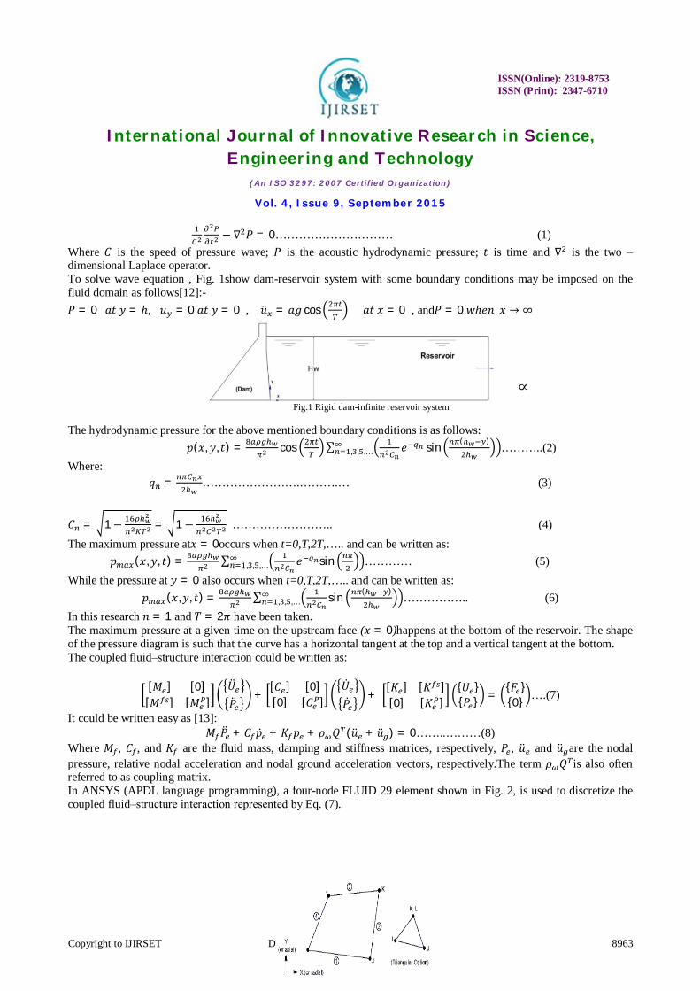
− ∇ 푃 = 0………………………… (1) Where 퐶 is the speed of pressure wave; 푃 is the acoustic hydrodynamic pressure; 푡 is time and ∇ is the two ‒ dimensional Laplace operator. To solve wave equation , Fig. 1show dam-reservoir system with some boundary conditions may be imposed on the fluid domain as follows[12]:- 푃 = 0 푎푡 푦 = ℎ, 푢 = 0 푎푡 푦 = 0 , 푢̈ = 푎푔 cos 푎푡 푥 = 0 , and푃 = 0 푤ℎ푒푛 푥 → ∞

Fig.1 Rigid dam-infinite reservoir system

The hydrodynamic pressure for the above mentioned boundary conditions is as follows:

푝(푥, 푦, 푡) = cos ∑ 푒 sin ( ), , ,… ………..(2)

Where: 푞 = …………………….……….… (3)

퐶 = 1− = 1− …………………….. (4)

The maximum pressure at푥 = 0occurs when t=0,T,2T,….. and can be written as: 푝 (푥,푦, 푡) = ∑ 푒 sin, , ,… ………… (5)

While the pressure at 푦 = 0 also occurs when t=0,T,2T,….. and can be written as: 푝 (푥,푦, 푡) = ∑ sin ( )

, , ,… …………….. (6) In this research 푛 = 1 and 푇 = 2휋 have been taken. The maximum pressure at a given time on the upstream face (푥 = 0)happens at the bottom of the reservoir. The shape of the pressure diagram is such that the curve has a horizontal tangent at the top and a vertical tangent at the bottom. The coupled fluid‒structure interaction could be written as:

[푀 ] [0][푀 ] [푀 ]

푈̈푃̈

+[퐶 ] [0][0] [퐶 ]

푈̇푃̇

+ [퐾 ] [퐾 ][0] [퐾 ]

{푈 }{푃 } =

{퐹 }{0} ….(7)

It could be written easy as [13]: 푀 푃̈ + 퐶 푝̇ +퐾 푝 + 휌 푄 (푢̈ + 푢̈ ) = 0……..………(8)

Where 푀 , 퐶 , and 퐾 are the fluid mass, damping and stiffness matrices, respectively, 푃 , 푢̈ and 푢̈ are the nodal pressure, relative nodal acceleration and nodal ground acceleration vectors, respectively.The term 휌 푄 is also often referred to as coupling matrix. In ANSYS (APDL language programming), a four-node FLUID 29 element shown in Fig. 2, is used to discretize the coupled fluid‒structure interaction represented by Eq. (7).

∞






Fig. 2 FLUID29Element Geometry[11] b- Soil-Structure interaction Modeling and analysis of dynamic soil structure interaction during earthquakes have gone through direct method (Global Method) where the soil and structure are included within the same model and analyzed in a single step [10].The discretized structural dynamic equation including the dam and foundation subject to ground motion can be formulated using the finite‒element approach as [13]:

푀 푢̈ + 퐶 푢̇ +퐾 푢 = −푀 푢̈ + 푄푝 …………………(9)

Where 푀 , 퐶 , and 퐾 are the structural mass, damping and stiffness matrices, respectively, 푢 is the nodal displacement vector with respect to ground and the term 푄푝 represents the nodal force vector associated with the hydrodynamic pressure produced by the reservoir. A four‒nodes PLANE 42 element (structural 2D solids) plain strain, shown in Fig. 3 which available in ANSYS is used for both dam body and soil foundation modeling.

Fig. 3 PLANE42 Element Geometry [11]

c- The Coupled Fluid-Structure-soilEquation The complete finite‒element discretized equations for dam-water-foundation interaction problem could be written from both Eqs. (8 and 9) in an assembled form as:

푀 0푀 푀

푈̈푃̈

+퐶 00 퐶

푈̇푃̇

+ 퐾 퐾0 퐾

푈푃 =

−푀 푈̈−푀 푈̈

…….(10)

Where 퐾 = −푄 and −푀 = 휌 푄 Eq.(10) expresses a second order linear differential equation having unsymmetrical matrices and may be solved by means of direct integration methods. In general, the dynamic equilibrium equation of systems modeled in finite elements can be expressed as: 푀 푢̈ + 퐶 푢̇ +퐾 푢 = 퐹(푡)……………….………(11) Where 푀 , 퐶 , 퐾 , and 퐹(푡) are the structural mass, damping, stiffness matrices and dynamic load vector, respectively. d- Model of Random Soil Properties The properties of random soil (퐶 and 휙 ) could be modeled using random field theory [14]. The soil cohesion, 퐶, is assumed to be lognormally distributed with mean 휇 , standard deviation 휎 , and spatial correlation length 휃 . The lognormal distribution is selected because it is commonly used to represent non-negative soil properties and since it has a simple relationship with the normal. A lognormally distributed random field is obtained from a normally distributed random field, 퐺 (푥), having zero mean, unit variance, and spatial correlation length 휃 through the transformation

푐(푥) = 푒푥푝{휇 + 휎 퐺 (푥)}……………………(12)






Where 푥 is the spatial position at which 퐶 is desired. The parameters 휇 and 휎 are obtained from the specified cohesion mean and variance using the lognormal distribution transformations

휎 = ln 1 + ……………………………..(13)

휇 = ln휇 − 휎 …………………………..(14) The friction angle, 휙 is assumed to be bounded both above and below, so neither normal nor lognormal distributions are appropriate. A beta distribution is often used for bounded random variables. Unfortunately, a beta distributed random field has a very complex joint distribution and simulation is cumbersome and numerically difficult. To keep things simple, a bounded distribution is selected which resembles a beta distribution but which arises as a simple transformation of a standard normal random field, 퐺∅(푥) according to

∅ + (∅ − ∅ ) 1 + tanh ∅( )……………..(15)

Where ∅ and ∅ are the minimum and maximum friction angles, respectively, and 푠 is a scale factor which governs the friction angle variability between its bounds. Fig.4 shows how the distribution of 휙 (normalized to the interval [0,1]) changes as 푠 changes, going from an almost uniform distribution at 푠 = 5 to a very normal looking distribution for smaller 푠 . In all cases, the distribution is symmetric so that the midpoint between ∅ and ∅ is the mean. Values of 푠 greater than about 5 lead to a U-shape distribution (higher at the boundaries), which is not deemed realistic. Thus varying 푠 between about 0.1 and 5.0 leads to wide range in the stochastic behavior of 휙. In this research푠is taken equal to 5.0

Fig.4 Bounded distribution of friction angle normalized to the interval [0,1] [14]

In this research the material properties of dam, reservoir, and foundation could be summarized in Table 1a, b, and cwhere represent the properties of concrete, water, and soil foundation,respectively:

Table 1a Dam Material properties

Properties Item

Density ρ (Kg/m3)

Modulus of elasticity Es

(Gpa)

Poisson's ratio ᶹ

Note

concrete 2400 25 0.2 Homogeneous, isotropic, and elastic properties of mass concrete are assumed.






Table 1b Reservoir Material properties

Properties Item

Density ρ (Kg/m3)

Bulk Modulus of elasticity Es

(Gpa)

Sonic velocity (m/s)

Note

water 1000 2.02 1440 Inviscid and compressible.

Table 1cFoundation Material properties [15]

Properties Item

Density ρ (Kg/m3)

Modulus of elasticity Es

(Mpa)

Poisson's ratio ᶹ

Cohesive of soil (C) (Kpa)

Angle of internal friction

ϕ°

Note

soil 1599 250 0.3 21.34 32.15 Tacked as a Random Soil

III. MODELING OF OPTIMIZATION PROBLEM BY ANSYS

The scheme of the practical section of dam with Somerfield–type radiation boundary conditionof reservoir and foundation that will be optimized by ANSYS can be given in Fig. 5[16],[9]and [17].

Fig. 5 Scheme of optimized dam model by ANSYS

Where 푯 is the total height, 푯풘 is the water height in the reservoir, 푯풖 is the upstream dam face slope height, 푯풅 is the downstream dam back slope height, 푩is the total dam base width, 풃풖 is the upstream dam face slope width, 풃풄is the dam crest width, and 풃풅 is the downstream dam back slope width. The optimization problem is to minimize the cost, therefore the adopted objective function implies on minimizing the volume of dam, and this implies the minimization of the dam section area, as given in Eq.(12)

푀푖푛 퐴 = ∗ + 푏 ∗ 퐻 + ∗ …………………….(12) Where each one of풃풖, 풃풄, 풃풅, 푯,푯풘, 푯풖,푯풅 is a design variable, while stress, strain, and displacement of the dam are considered as state variables. The factors of safety that should be realized for stability and safety after optimization process will be finished could be given as [18], [19],and[20]:

1. Against sliding, 퐹푂푆 =

= ∑∑ > 1.5 ……………..…(13)

2. Against Overturning,퐹푂푆 =

= ∑

∑ > 2 …..…...(14)






3. Bearing capacity of soil,퐹푂푆 = =

∑ ∓ ≥ 3…..…...(15)

Where퐶푁 + 푞푁 + 훾 퐵 푁 is Terzaghi's bearing capacity, and퐵 = 퐵 − 푒 and 푒 is the eccentricity. If the soil is replaced by a pile to bear the coming loads, in this case

푞 = 푞 + 푞 ……………………….(15-a) Where: 푞 = ultimate bearing capacity of pile (KN/m2),푞 = theoretical bearing capacity for tip of foundation, or end bearing (KN/m2), 푞 = theoretical bearing capacity due to shaft friction, or adhesion between foundation shaft and soil (KN/m2). Also, 푞 = 푄

퐴 , 푞 = 훾 ℎ 푁 (푓표푟 푐표ℎ푒푠푖표푛푙푒푠푠 푎푛푑 푠푖푙푡 푠표푖푙 ) ,푞 = 9퐶 ( 푓표푟 푐표ℎ푒푠푖푣푒 푠표푖푙푠 )…(15-b) Where: 푄 is thetheoretical bearing capacity for tip of foundation, or end bearing (KN),퐴 is thecross-section area (m2), in which 퐴 = 휋

4 × 퐷 , 퐷 is the diameter of a pile (m), 훾 is the unit weight of soil (KN/m3),ℎ is the effective depth of pile (m), 푁 is the bearing capacity factor for soil, 퐶 is the cohesion of soil (KN/m2).While,

푞 = 푄퐴 ….. …………………….….…(15-c)

Where:푄 is the theoretical bearing capacity due to shaft friction, or adhesion between foundation shaft and soil (KN), 퐴 is the surface area of a pile that the adhesion with a soil may be happened (m2), in which퐴 = 푃 × 퐿, 푃 is the perimeter of pile cross‒section (m)and 푃 = 휋퐷for circular pile or 푃 = 4퐷 for square pile;퐿 is the effective length of pile (m).In other hand, 푞 = 퐾푆 tan 휆for cohesion less soils (KN/m2), 푞 = 퐶 +퐾푆 tan 휆 for soil silts(KN/m2), and 푞 = 푎 푆 for cohesive soils (KN/m2). Where:푆 is a cohesion factor (KN/m2), Also: 푎 = 1− 0.1(푆 ) for푆 < 48퐾푁/푚 cohesion factor, 푎 = [0.9 + 0.3(푆 − 1)]for푆 > 48퐾푁/푚 푆 = 2퐶= unconfined compressive strength (KN/m2) 퐶 is the adhesion , so 퐶 = 퐶 for rough concrete, rusty steel, corrugated metal ; while 0.8퐶 < 퐶 < 퐶 for smooth concrete; in other hand, it may be 0.5퐶 < 퐶 < 0.9퐶 for clean steel. 휆is the external friction angle of soil and wall contact (degree) 푆 = 푔퐷it is the effective overburden pressure (KN/m2) 퐾 =lateral earth pressure coefficient for piles.

4. Exit gradient (seepage), 퐹푂푆 = = ⁄⁄ ≥ 1 ………….……..(16)

Where 퐺 is the specific gravity of soil and is equal to 2.7, and 푒 is the void ratio and equal to 0.60 [15] 5. Shear stress of soil should don’t exceed allowable shear stressof soil. Therefore, in this paper 휏 = 푞 ∗ tan훽……….…………………….(17)

Where 훽 is the inclination of upstream face of dam with vertical axes, and allowable shear stressof soil is equal to 0.79 Mpa.

6. The crack section should be avoided. The resultant force must passes through middle third of the dam width i.e. 푒 <

7. Liquefaction process on the foundation when the soil is sand and saturated must be prevented. In this paper, the selected site of the optimized dam may be on east regionof Iraq with Iran boundary.The topographic of this region is shown in Fig.6.






Fig. 6 Topographic of Iraq and site region of study [15]

Therefore, the height of water in the reservoir 푯풘for this region is found to be 15m and the practical section that is used roughly in design could be given according to the variablesratio in Table 2[21].

Table 2 Variables Ratio After[21]

Variables Ratio

Range Values Adopted

Max. Ava. Min.

퐵/퐻 0.75-0.85 0.75 0.80 0.85

퐻 /퐻 0.85-0.95 0.85 0.90 0.95

퐻 /퐻 0.50-0.70 0.50 0.60 0.70

퐻 /퐻 0.80-0.90 0.80 0.85 0.90

푏 /퐵 0.063-0.088 0.063 0.0755 0.088

푏 /퐵 0.093-0.15 0.093 0.1215 0.15

푏 /퐵 0.788-0.84 0.788 0.80 0.84 The average variables ratio in Table (2) is tacked as an initial value for the model in optimization problem. Then, the design variables (DVS) are set to the following constraints:

(퐻 = 퐻 /0.95) ≤ 퐻 ≤ (퐻 = 퐻 /0.85) (퐻 = 0.50퐻) ≤ 퐻 ≤ (퐻 = 0.70퐻) (퐻 = 0.80퐻) ≤ 퐻 ≤ (퐻 = 0.90퐻)

(푏 = 0.063퐵) ≤ 푏 ≤ (푏 = 0.088퐵)………………….(18) (푏 = 0.093퐵) ≤ 푏 ≤ (푏 = 0.15퐵) (푏 = 0.84퐵) ≤ 푏 ≤ (푏 = 0.788퐵)

퐵 = 푏 + 푏 + 푏






IV. LOADS OF OPTIMIZATION PROBLEM

In the design of concrete gravity dam, it is essential to determine the loads required in the stability and stress analyses which are weight of dam , water pressure (static and dynamic) ,uplift forces , earthquake forces , and seismic load .The forces of wind waves, silt, and Ice are ignored in this research.Fig. 7 shows these forces . The seismic load is concerned according to the records of earthquake stations placed on the region of study. Therefore, the records of Badra station on Amara City [22], is transformed as time-history force as shown in Fig.8

Fig. 7 Loads on optimization dam model

Fig. 8 Earthquake time-history force

V. RUNNING OF OPTIMIZATION PROBLEM BY ANSYS

The scheme of ANSYS APDL steps of the modeling of the optimization process including dam‒reservoir‒foundation interaction under seismic effect could be shown in Fig. 9

Fig 9 Scheme of ANSYS APDL modeling






The 2D finite element model of the optimization problem using ANSYS APDLis given in Fig. 10. It is shown from the figure the discretization of model and the interaction among dam-reservoir-foundation interaction, the fixed boundary, and applied loads.

Fig. 10 Finite element discretization model of optimization process

In this research, the individual-accumulative optimization process is developed. This process aim to carry out each constraint individually through the optimization process. Therefore, the modified sectionsare provided to reach the final optimum section.

VI. RESULTS AND DISCUSSIONS

After the optimization process is conducted, the initial, modified, and optimum sections of dam are given in Table 3. As noticed in this table, The feasible sections and modified feasible sections represent the feasible or alternative sections obtained from the optimization process.

Table 3 Initial and Optimum Dimensions

Also, the optimal variables ratio that obtained after optimization process is finished are given in Table 4. These ratio will be depended on the design of dam to give more economic section.

Table 4Variables Ratio

VariablesRatio hw/H B/H hu/H hd/H bu/B bc/B bd/B Initial 0.90 0.80 0.60 0.85 0.0799 0.1214 0.80 Optimal 0.83 0.72 0.83 0.65 0.0639 0.1216 0.81

In other hand, R.C. piles are considered in the optimization process in two cases. The first one; case-1; the piles serve as a barrier to reduce seepage beneath a dam, and as a structure to improve bearing capacity that sufficientto bear the dam. The optimum details of number, type and dimensions of these piles are given Table 5.






Table5Details of piles for case-1

DP (m) lP (m) No. lP / DP lP/ B Type of pile FOS)bearing capacity 1.00 2.53 1 2.53 0.13804 Secant Pile 3.000 0.90 2.85 1 3.166 0.15518 Secant Pile 3.000 0.80 3.22 1 4.025 0.17550 Secant Pile 3.000 0.70 3.67 1 5.24 0.2000 Secant Pile 3.000 0.60 4.22 1 7.033 0.23010 Secant Pile 3.000 0.50 4.92 1 9.84 0.26820 Secant Pile 3.000 0.40 5.85 1 14.625 0.31870 Secant Pile 3.000 0.30 7.17 1 23.90 0.39059 Separate Pile 3.000

The second; case-2; where the piles serve as well mentioned in case-1 as a key beneath a dam to overcome both sliding and overturning. All details related these piles which may be as separate piles with space in between them or may be as secant piles are given in Table 6.

Table 6 Details of piles for case-2

DP (m) lP (m) No. lP / DP lP/ B Type of pile FOS)bearing capacity 1.00 3.40 1 3.40 0.24156 Secant Pile 3.000 0.90 3.79 1 4.21 0.26923 Secant Pile 3.000 0.80 4.25 1 5.31 0.30182 Secant Pile 3.000 0.70 4.80 1 6.85 0.34098 Secant Pile 3.000 0.60 5.47 1 9.11 0.38857 Secant Pile 3.000 0.50 6.31 1 12.62 0.44824 Secant Pile 3.000 0.40 7.43 1 18.57 0.52781 Secant Pile 3.000 0.30 9.01 1 30.03 0.6400 Separate Pile 3.000

The individual - accumulative optimization processissuggested by authors to include each constraint individuallyin the optimization process. This lead to constructmultiple loops in order to get the optimal solution in final of optimization process. Consequently, the initial, feasible, modified, and optimal sections details could be shown in Fig.11.






Fig.11 Optimization Process

VII. CONCLUSIONS

The section of concrete gravity dam should be chosen in such a way that it is the most economic section and satisfies all the conditions and requirements of stability and safety. It is found from the results the following:-

1. The ANSYS APDL is efficient tool to simulate dam-reservoir-foundation interaction problem and optimization process.

2. The optimization process is suitable technique to get the optimum section. 3. The individual - accumulative optimization process gives reasonable procedure to carry out the factors of

safety individually. 4. The initial section of dam that is provided according toinitial variables ratios is not representing the optimum

section because of falling of factors of safeties. 5. The optimum section of a dam on random soil is obtained with piles serve in the same time as a bearing

capacity improvement device, a seepage control device, and a key underneath a dam in order to overcome both sliding and overturning.






REFERENCES

[1] Dey, A., and Sawant, M.B.,"Seismic Response of a Concrete Gravity Dam Considering Hydrodynamic Effects", APCOM & ISCM, Singapore, 2013. [2] Gao, L., JianGuo, D., and ZhiQiang, H., "Dynamic dam-reservoir interaction analysis including effect of reservoir boundary absorption", School of Civil and Hydraulic Engineering, Dalian University of Technology, Dalian 116024, China Science in China Series, Springer, 2007. [3]Pasbani-Khiavi, M., Gharabaghi, A.R.M., and Abedi, K., "Dam-Reservoir Interaction Analysis Using Finite Element Model", The 4th World Conference on Earthquake Engineering, October 12-17, Beijing, China, 2008. [4] Singh, B., and Agarwal, P., "Seismic Response of High Concrete Gravity Dam Including Dam-Reservoir-Foundation Interaction Effect", J. of South Asia Disaster Studies, Volume 02, Issue 02, pp. 41-57, 2009. [5] Das, K., Das, P. K. , and Halder, L., "Seismic Response of Concrete Gravity Dam ", Natinal Institute of Technology Agartala NIT, India , 2011. [6] Khan, S., and Sharma, V. M., "Stress Analysis of a Concrete Gravity Dam with Intersecting Galleries", International Journal of Earth Sciences and Engineering, Vol. 04, Issue 06, 2011. [7] Heydari, M. M., and Mansoori, A., "Dynamic Analysis of Dam-Reservoir Interaction in Time Domain", J. of World applied sciences, Vol.15, Issue10, pp. 1403-1408, 2011. [8] Salmasi, F., "Design of Gravity Dam by Genetic Algorithms", International Journal of Civil and Environmental Engineering,Vol.03,Issue03, pp.187-192,(2011). [9] Salajegheh, J. and khosravi,S.,"Optimal Shape Design of Gravity Dams Based on a Hybrid Meta-Heruristic Method and Weighted Least Squares Support Vector Machine", International Journal of Optimization in Civil Engineering,Vol.04, pp. 609-632, 2011. [10] Berrabah, A., T., "Dynamic Soil‒Fluid‒Structure Interaction Applied for Concrete Dam", PhD thesis, University of AboubekrBelkaïdTlemcen, Algeria, 2012. [11] ANSYS. ANSYS User's Manual, "ANSYS Theory Manual'', Version 11.0, 2009. [12] Ghaemian, M., "Course Notes, Chapter 2: Reservoir", Indian Institute of Technology, WWW.Sharif.edu.com, 2000. [13] Khosravi, S., Salajegheh, J., and Heydari, M. M.,"Simulating of Each Concrete Gravity Dam with Any Geometric Shape Including Dam-Water Foundation Rock Interaction Using APDL", World Applied Sciences Journal, Vol.17, Issue03, pp.1818-4952, 2012. [14] Fenton, G. A. and Griffiths, D.V.,"Bearing Capacity Prediction of Spatially Random 푐 ‒ 휙 soils ", J. of Canadian Geotechnical, Vol. 40, Issue01, pp. 54-65, 2003. [15] Center of Studies and Engineering Design (CSED), “Investigations Report of Al-Teeb Dam: Meesan Governorate”, Ministry of Water Resources, Iraq , 2011. [16] Ali, A. A. M., Al-Suhaili, R. H. S., and Behaya, Sh. A. K., "A Genetic Algorithm Optimization Model for the Gravity Dam Section under Seismic Excitation with Reservoir-Dam-Foundation Interaction", American Journal of Engineering Research (AJER), Vol.03, Issue06, pp. 143-153, 2014. [17] Duggal, K. N., and Soni, T. P., "Elements of water Resources Engineering: Gravity Dams Part 2: Stability Analysis", New Age International Publishers, Indian, 2005. [18] Al-Janaini, M. A., "Hydraulic Structures", Al-Ratib for the Universal-Researches, Beirut, [In Arabic], 1980. [19] USBR (United State Department of the Interior, Bureau of Reclamation), “Design of Small Dams”, 3rd Edition, U.S. Government Printing Office, Washington, USA, 1987. [20] Tomlinson, M. J.,"Pile Design and Construction Practice", E & FN SPON, London, UK, 1994. [21] Behaya, S. M. K., "Optimum Dimensions of Concrete Gravity with Fluid‒Structure‒Foundation Interaction Under Seismic Effect", PhD Thesis, Water Resources Eng. Dept., College of Engineering, University of Bagdad, Bagdad, Iraq, 2014. [22] Iraqi Meteorological Organization and seismology (IMOS), “StationsRecords”, Ministry of Transportation, Baghdad, Iraq, 2013.

Documents

Optimum Design of Low Concrete Gravity Dam on Random Soil ...ijirset.com/upload/2015/september/95_Optimum_NEW.pdf · In the latest decade, dynamic analysis of concrete gravity dam