Embed Size (px)
Citation preview

J. Agr. Sci. Tech. (2021) Vol. 23(5): 1163-1178
1163
1 Department of Hybrid Seed Production, Iranian Company for Maize Development, Tehran, Islamic
Republic of Iran. 2 Department of Soil Science, Faculty of Agricultural Engineering and Technology, College of
Agriculture and Natural Resources, University of Tehran, Islamic Republic of Iran.
* Corresponding author; e-mail: [email protected] 3 Department of Agronomy and Plant Breeding, Faculty of Agricultural Sciences and Engineering,
College of Agriculture and Natural Resources, University of Tehran, Islamic Republic of Iran. 4 Atmospheric Science and Meteorological Research Center, Tehran, Islamic Republic of Iran.
Optimum Cropping Pattern Based on Irrigation Water
Productivity Using AquaCrop Simulation Model
A. Izadfard1, F. Sarmadian2*, M. R. Jahansooz3, and E. Asadi Oskouei4
ABSTRACT
Optimum cropping pattern increases productivity where input resources are limited.
An optimized cropping pattern was developed for a region in Moghan Plain, located in
the northwestern Iran, to help water supplier in pre-season decision making on water and
land allocation. AquaCrop simulation model was calibrated and executed for yield
predictions for 11 different crops and 13 diverse soil types. Evaluation of AquaCrop
model showed great robustness for a broad range of crops, even for the crops like canola
and alfalfa that were undefined for the model. The precise generated crop water functions
revealed the ideal conditions for water allocation by considering the impact of the existing
limitation in monthly water availability on optimum cropping pattern without imposing
any manipulation. Optimum cropping pattern based on water productivity (OCPWP) was
identified by LINGO software. Integrating AquaCrop model and LINGO optimization
problem solver created a Decision Support System (DSS) for technical analysis at the
regional level. The created DSS is able to support the OCPWP in terms of the complex
regional crop-mixture acreage. The ecological considerations introduced diverse winter
crops to benefit from autumn precipitations. This strategy decreases irrigation
requirement and saves some water for spring/summer high water-demanding crops like
alfalfa and cotton, which generally enhances the system resiliency. The generated DSS
revealed that 8,762 m3 water ha-1 was required for optimum cropping pattern, which is
8% lower than the maximum and 3% more than the average available water.
Keywords: Crop per drop index, Decision support system, System resiliency.
INTRODUCTION
Water is the most widely existing natural
resource on our planet, although about
97.5% of it is saline. However, only a small
fraction is available as freshwater
(Shiklomanov, 2000). Freshwater is an
indispensable natural resource, which plays
a vital role in the development of any
country. Presently, many countries of the
world are experiencing scarcity of fresh
water (Mekonnen and Hoekstra, 2016). This
finite freshwater resource supports life on
the planet, and is threatened by population
growth, pollution, and food demands.
Therefore, an integrated water management
strategy is necessary to avoid the risks of
water scarcity (Poff et al., 2016). Failure to
develop such a strategy will intimidate
health, social and economic well-being, food
security, biodiversity and generally
promotes human conflicts. As a result,
optimal water allocation has become one of
the most confusing challenges faced by
policy makers. Freshwater scarcity develops
Dow
nloa
ded
from
jast
.mod
ares
.ac.
ir at
13:
52 IR
ST
on
Tue
sday
Nov
embe
r 30
th 2
021
______________________________________________________________________ Izadfard et al.
1164
not only from the physical constraints but
also due to inefficient water uses and poor
management, which has widened the gap
between the water sources and sinks in most
parts of the world (Simonovic, 2002).
Optimum cropping pattern is a key to close
the gap between water supply and water
demand.
In many water-scarce countries like Iran,
the agricultural sector is the main water
consumer that withdraws the main quota of
all available freshwater at insufficient water
use efficiency (Motiee et al., 2001). Some
studies have predicted a 14% net increase in
the use of water to meet the food demands
by the year 2030 compared to 2000
(Rockström et al., 2007). Hence, pursuing
sustainable technique to increase crop water
productivity along with preserving the soil
and water resources, is gaining prominence
in arid and semiarid regions of the world.
Optimum cropping pattern, as a sustainable
management technique, could shift the focus
on maximizing total production to
maximizing water productivity (Debaeke
and Aboudrare, 2004; Sepulcre-Cantó et al.,
2007). Optimum cropping pattern is directly
related to the productivity of irrigation
systems and greatly contributes to soil and
water utilization (Sethi et al., 2002).
Furthermore, optimal cropping pattern
interacts with water requirement and crop
yield, as well as optimal profitability.
Therefore, cropping pattern plays an
important role in rural economic
development through its impacts on
increased income levels and water use
efficiency (Montazar and Rahimikhob,
2008). Analyzing crop responses to water is
a multi-variable process, because it depends
on soil characteristics, weather conditions,
crop growth behaviors, planting dates, farm
management, and many other circumstances.
Crop simulation models are designed to
imitate the behavior of such a complex
system (Hoogenboom, 2000). Crop
simulation models study the plant response
to different combinations of resources and
interactions with time phenomena.
AquaCrop is a water-driven simulation
model that requires a relatively low number
of parameters and input data to simulate the
yield response to water of major crops
cultivated worldwide. The limited AquaCrop
inputs are the key elements to investigate
and determine the plant response to different
resource management while maintaining the
sufficient balance between accuracy,
simplicity, and robustness (García-Vila et
al., 2009; Katerji et al., 2013; Mkhabela and
Bullock, 2012; Rankine et al., 2015;
Wellens et al., 2013). AquaCrop simulates
attainable yields of major herbaceous crops
as a function of required water under various
irrigation conditions in the atmosphere–
plant-soil system (Steduto et al., 2009). The
growth engine of AquaCrop is water-driven,
which initially separates ET into soil
evaporation and crop transpiration, then
translating the crop transpiration into
biomass using conservative, crop-specific
parameters. The separation avoids the
confounding effect of non-productive water
requirement (Geerts et al., 2010). AquaCrop
model generates normalized crop water
productivity (Steduto et al., 2007) which is
the model’s key approach for applicability in
different locations under varying spatio-
temporal settings (Steduto and Albrizio,
2005).
Cropping pattern considers regional water
and land allocations among different crops.
Nonlinear programming models can be used
as effective tool to optimize cropping pattern
for both ecological and economic goals in
the command areas. In crop production
system, Water Use Efficiency (WUE) is
used to define the crop production per unit
volume of water (Ali and Talukder, 2008).
WUE refers to the ratio between the final
dry matter yield and cumulative crop
evapotranspiration. WUE is a useful
indicator for quantifying the impact of water
management. Water production function is a
key output of crop simulation models from
which the yield response to water is
regularly simulated with empirical functions
(Goldhamer and Fereres, 2017).
The objective of the present study was to
develop and execute a nonlinear
Dow
nloa
ded
from
jast
.mod
ares
.ac.
ir at
13:
52 IR
ST
on
Tue
sday
Nov
embe
r 30
th 2
021

Optimum Cropping Pattern Based on Water Productivity ___________________________
1165
Figure 1. Location of the study area as a part of Moghan Plain in northwest of Iran.
Study Area
optimization model to determine an optimal
cropping pattern based on WUE by Crop Per
Drop (CPD) index. CPD index is the total
crop yield per one cubic meter of total water
used (Monaghan et al., 2013). For this
purpose, the crop water productivity
function is combined with the CPD index as
an objective function of the optimization
model to design the optimum cropping
pattern for part of the Moghan Plain in Iran.
MATERIALS AND METHODS
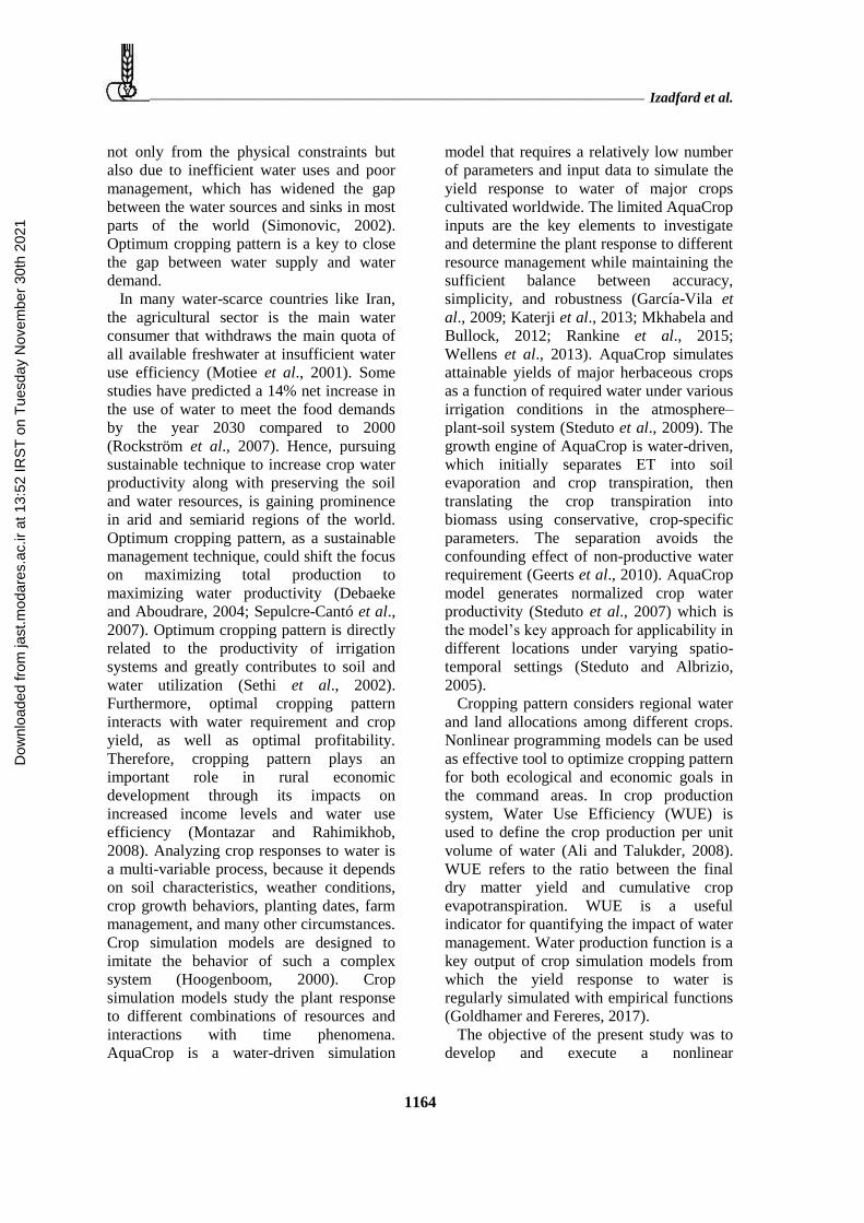
Description of the Study Area
The study area is a newly developed part
of the Moghan Plain located at 47° 33' 18"
to 47° 52' 32" E Longitude, 39° 21' 05" to
39° 33' 06" N Latitude, 180 to 330 m above
mean sea level, in Ardabil province,
northwest of Iran (Figure 1). The Moghan
Plain is one of the major agricultural regions
in Iran (Nasseri et al., 2006). Currently,
dryland agriculture is practiced in the main
parts of the study area. The area is irrigated
through Khodaafarin dam, which is
constructed on the Aras River. Due to the
land slope and topography, the sprinkler
irrigation system is applied. In this study, 11
irrigated crops were chosen according to the
regional policy and climatic conditions. The
crops included wheat, barley, canola, and
sugar beet in winter, cotton, grain maize,
soybean and alfalfa in spring and soybean,
grain maize and silage maize in summer.
Climate and Soil Data
Moghan Plain has a semi-arid climate with
relatively high Evapotranspiration (ET).
Previous 20-year climate data were obtained
from the nearest weather station (39° 39' N,
47° 55' E, 32 m above mean sea level) in
Parsabad City (Figure 2). Based on a recent
soil survey, an area of 12,004 ha is covered
by 13 different soil types with different
characteristics including salinity, hardpan,
and slope, (Table 1). The soil survey
provides soil classification and physical and
chemical properties at different depth
intervals of 0.15 m to a depth of 1.5 m
(Seyedmohammadi et al., 2018). The
irrigation water with relatively moderate
salinity (1.1 dS m-1) causes soil salinity and
imposes a reduction in crop yield.
The runoff Curve Number (CN) of each
soil series was calculated based on the soil
series physical characteristics to estimate
surface runoff from rainfall that occurred
during the simulation period. According to
the soil series slope, the soils are divided
into four groups (A, B, C and D)
Dow
nloa
ded
from
jast
.mod
ares
.ac.
ir at
13:
52 IR
ST
on
Tue
sday
Nov
embe
r 30
th 2
021

______________________________________________________________________ Izadfard et al.
1166
representing land slopes of 0-2, 2-5, 5-8 and
8-12%, respectively.
Regional Crop Data
Data of crops water consumptions were
collected from local experts (Table 4) and
crop phenology data were obtained from
Oltan Agrometeorological Research Station
(39° 36.217' N; 47° 46.733' E, 72 m above
mean sea level) located near the study area. -
In the present study, according to the local
information, the simulations were conducted
with sprinkler irrigation, 50% depletion of
available moisture and 100% wetted area.
Moreover, total irrigation efficiency was
assumed to be 65%. All crops have their
built-in crop parameters in AquaCrop,
except canola, silage maize, and alfalfa.
Canola and silage maize are already
calibrated (Hsiao et al., 2009; Salemi et al.,
2011; Zeleke et al., 2011). A leafy crop
using AquaCrop multiple run project was
defined to simulate alfalfa for five cutting
cycles (Allen et al., 1998). The crops’
optimum planting dates were previously
calibrated for the region (Izadfard et al.,
2017).
AquaCrop Calibration
AquaCrop version 5.0 (available at
http://www.fao.org/aquacrop/en) was used
in this study, and all simulations were
implemented in the degree-day mode. For
the simulations, soil fertility was considered
near optimal (about 80%) to cope with the
real situation. Runoff was considered by the
model based on each soil characteristics.
The model calibration was performed by
using the observed values from Oltan
Agrometeorological Research Station during
2013–2014 cropping seasons. The dry
matter yield output of the simulations was
Figure 2. (a) Minimum and maximum temperatures and (b) Evapotranspiration and precipitation in Moghan
Plain based on historical data (January 1994 to December 2013).
Dow
nloa
ded
from
jast
.mod
ares
.ac.
ir at
13:
52 IR
ST
on
Tue
sday
Nov
embe
r 30
th 2
021

Optimum Cropping Pattern Based on Water Productivity ___________________________
1167
Table 1. Soil series physical, chemical and hydraulic characteristics in the study area.
MA
1/
0-2
%
slo
pe
Depth (cm) Texture Saturation (%) EC (dS m-1) pH OM (%) FC at 33.3 kPa WP At 1500 kPa BD (g cm-3)
0-20 CL 57.0 1.41 7.81 1.56 29 20 1.41
20-35 CL 45.0 0.56 7.87 0.52 26 19 1.33
35-75 SL 29.0 1.07 7.66 0.20 18 12 1.40
75-120 SCL 52.0 2.90 7.68 0.16 24 17 1.33
120-170 C 79.0 5.81 7.84 0.00 31 23 1.30
HH
3/
2-5
%
slo
pe
0-20 CL 52.0 1.07 7.78 1.22 27 18 1.44
20-52 C 61.0 8.28 7.72 0.46 32 24 1.31
52-72 C 61.0 1.34 8.11 0.38 33 25 1.29
72-91 C 62.0 12.46 7.63 0.19 33 25 1.30
91-110 C-CL 56.0 10.68 7.68 0.08 30 21 1.36
110-150 CL 54.0 10.68 7.59 0.00 27 19 1.39
MT
1/
2-5
%
slo
pe
0-10 SL 33.0 0.89 7.71 1.07 20 14 1.37
10-31 LS 38.0 0.53 7.86 0.23 15 10 1.50
31-41 SL 33.0 0.53 7.84 0.27 19 13 1.38
41-49 LS 35.0 0.50 7.82 - 15 10 1.50
58-81 SL 36.0 2.31 7.61 0.30 20 14 1.40
110-150 SiC 60.0 5.61 7.70 0.68 33 23 1.38
KO
4/
2-5
% s
lop
e
0-30 CL 51.0 0.89 7.21 1.00 29 20 1.41
30-65 C to CL 48.0 2.24 7.54 0.24 30 21 1.37
65-97 CL 50.0 1.74 7.96 0.04 28 20 1.37
97-125 SiCL 46.0 8.30 7.60 0.04 30 20 1.44
125-150 SiCL 45.0 9.13 7.64 0.00 30 19 1.49
GL
2/
2-5
%
slo
pe
0-11 CL 49.0 1.91 7.81 1.16 29 19 1.48
11_30 SiCL 49.0 0.81 7.93 0.60 30 21 1.41
30-66 SiC 49.0 1.17 7.86 0.28 32 24 1.34
66-74 SiC 48.0 2.10 7.77 0.15 21 14 1.48
74-100 SL 44.0 3.99 7.76 0.04 22 13 1.47
100-150 L 40.0 2.41 7.71 0.04 25 14 1.58
DE
1/
2-5
% s
lop
e
0-20 SiC 56.0 0.98 7.57 1.07 32 22 1.39
20-50 SiC 53.0 0.74 7.93 0.61 32 23 1.37
50-105 SiC 49.0 2.67 8.29 0.04 32 24 1.35
105-112 SiC 50.0 3.50 7.86 0.04 29 19 1.51
112-150 CL 50.0 5.79 7.48 0.00 26 18 1.42
GG
2/
8-
12
%
slo
pe
0-20 SiCL 58.0 1.17 8.25 0.32 30 18 1.53
20-42 SiCL 48.0 0.53 7.81 0.64 31 21 1.43
42-100 SiCL 50.0 0.81 7.70 1.32 31 21 1.43
100-150 SiCL 52.0 9.96 7.79 0.31 30 21 1.44
SK
1/
2-5
%
slo
pe
0-30 SiCL 50.0 0.68 7.68 1.44 31 20 1.49
30-62 SiC 64.0 2.07 8.12 0.24 33 24 1.35
62-69 SiC 62.0 3.40 7.89 0.15 29 19 1.51
69-80 SiCL 59.0 10.80 7.64 0.12 30 20 1.43
80-115 SiCL 57.0 14.94 7.51 0.01 31 21 1.42
115-150 SiC to C 57.0 10.79 7.75 0.00 34 25 1.32
KH
1/
2-5
%
slo
pe
0-20 CL 51.0 2.67 7.50 1.25 29 20 1.37
20-40 C 50.0 0.67 7.70 0.61 30 23 1.31
40-70 CL 47.0 0.98 7.73 0.27 28 20 1.37
70-76 CL 48.0 1.50 7.70 0.15 27 19 1.42
76-110 C-CL 54.0 3.38 7.65 0.04 29 21 1.32
110-150 C-CL 48.0 5.87 7.68 0.11 28 22 1.27
HA
2/
2-5
% a
nd
HA
3/
5-8
%
slo
pe
0-20 SiC-C 61.0 1.66 7.59 1.56 33 24 1.34
20-47 C 96.0 1.16 8.37 0.92 35 27 1.26
47-71 C 86.0 10.79 7.83 0.64 36 28 1.25
71-91 C 74.0 18.26 7.48 0.44 34 26 1.28
91-150 C 80.0 14.11 7.46 0.32 36 28 1.25
MV
3/
2-5
% a
nd
MV
4/
5-
8%
slo
pe
0-20 C 56.0 2.59 7.66 0.38 33 25 1.29
20-40 C 58.0 2.41 7.71 0.19 32 25 1.25
40-70 C to CL 63.0 2.67 7.90 0.15 36 29 1.22
70-115 C 64.0 4.28 8.00 0.00 36 28 1.23
115-150 C 71.0 5.34 8.20 0.00 36 28 1.24
OC= Organic Matter BD= Baulk Density L= Loam C= Clay CL= Clay Loam
FC= Field Capacity SiC= Silty Clay SL= Sandy Loam LS= Loamy Sand SCL= Sandy Clay Loam
WP= Wilting Point SiCL= Silty Clay Loam
Dow
nloa
ded
from
jast
.mod
ares
.ac.
ir at
13:
52 IR
ST
on
Tue
sday
Nov
embe
r 30
th 2
021

______________________________________________________________________ Izadfard et al.
1168
converted to actual yield using moisture
content values of 15, 14, 75, 11, 12, 14, 15,
80 and 17% for wheat, barley, sugar beet,
canola, cotton, soybean, grain maize, silage
maize and alfalfa, respectively. The
difference between the predictions and
observations were minimized by mostly
manipulating canopy cover and harvest
index using trial and error approach (Steduto
et al., 2009).
Model Evaluation
Regional crop yield and water requirement
were considered in this study for model
evaluation. Three statistical indices
including coefficient of determination (R2),
Normalized Root Mean Square Error
(NRMSE) and d index were employed to
compare the simulated results against the
observed data. The NRMSE gives a measure
of the relative difference of simulated versus
observed data. The simulation is considered
excellent if NRMSE is less than 10%, good
if less than 20%, fair if greater than 20, and
poor if greater than 30 (Andarzian et al.,
2011). The agreement index d represents the
agreement between the observed and
predicted observations (Willmott, 1981). It
overcomes the insensitivity of R² or
underestimations by the model. It ranges
between 0 and 1, with 0 indicating no
agreement and 1 indicating a perfect
agreement between the predicted and
observed data (Legates and McCabe, 1999;
Willmott and Matsuura, 2005).
NRMSE = [∑(Pi−Oi)2
n
n
i=1]
1/2
×100
M (1)
d = 1 − [∑ (Pi−Oi)2n
i=1
∑ (|Pi′|−|O′
i|)2n
i=1
] (2)
CPD DSS Formulation
All 143 functions comprised by 11 crops
and 13 soil types were produced by the
LINGO software version 11, available at
http://www.lindo.com. The yield of each
crop can be obtained through crop water
production function based on average water
requirement for all soil series during the
whole growth period. As the generated
functions show, crop biomass water use
efficiency was determined by the slope of
each crop water production function. The
water use efficiency developed by
AquaCrop model integrates the precipitation
and soil water content. The main
optimization function (Z) has been
comprised by 143 crop/soil functions (11
crops×13 soil types). The average crop water
requirement for each crop was introduced to
the main optimizing model. The comparable
yield of each crop/soil function was
calculated using average irrigation water
requirement. By introducing the average
crop water requirement to the main function,
the optimum acreage for each crop was
determined. In order to optimize the water
use efficiency of each crop/soil unit, the
main objective functions were formulated
based on all crop/soil units for CPD index
and monthly crop water requirement indices.
The constraints imposed on the objective
function of the model were total available
Water (W), monthly available water (m),
Total area (TL), each soil series area (sL),
first and second crop Production function
(P) in a year, optimum acreage of each crop
(S) and calculated CPD index (A). Ten
percent of the total land was considered
under fallow. Maximizing the main function
(Z) based on the constraints was computed
by LINGO software. While the total land,
total water, monthly water, and each
crop/soil CPD are constant, individual crop
acreage and consequently crop production
need to be optimized to determine maximum
production of total area. Some studies have
shown that crop water function optimization
can be more accurately solved by nonlinear
structures compared to linear methods
(Barati et al., 2020; Zhao et al., 2017).
ij
i
ijij
j
SPAZMax
11
1
13
1 (3)
TLSj
j
13
1 (4)
Dow
nloa
ded
from
jast
.mod
ares
.ac.
ir at
13:
52 IR
ST
on
Tue
sday
Nov
embe
r 30
th 2
021

Optimum Cropping Pattern Based on Water Productivity ___________________________
1169
sLSj
j
13
1 (5)
WSPA ij
i
ijij
j
11
1
13
1 (6)
mSPA ij
i
ijij
j
11
1
13
1 (7)
RESULTS AND DISCUSSION
Calculation of ETo is a critical parameter
for model accuracy. In the current study, the
available climatic parameters including solar
radiation, wind speed, air pressure,
temperature and precipitation were used to
calculate ETo in FAO ET calculator (Raes
and Munoz, 2009). The annual temperature
range is acceptable for most of the crops
from January to July. The 271 mm annual
precipitation compared to 2,221 mm of ETo,
is not enough for dry farming system, except
for wheat and barley.
Fine-Tuned Model
AquaCrop model was fine-tuned for 11
different field crops under full irrigation
based on the obtained phenology data. The
calibrated parameters are shown in four
different factor groups in Table 2. The
simulated yields were compared to the
corresponding regional crop yields. As
illustrated in Table 3, sugar beet showed the
best model performance by NRMSE= 10.33,
R2= 0.93 and d Index= 0.88. It could be
resulting by adding up the sugar beet-related
high moisture content, which reduces the
bias of error in dry mass simulation. On the
other hand, cotton showed the weakest
result, which could be the result of using
local cotton variety with different growth
habits. The same conclusion has been
reported for local cotton varieties (Farahani
et al., 2009). What is clear from Table 3 is
the weakness of R2 as a single statistical
factor for model performance.
It should be noted that the NRMSE and d
index tended together and the low NRMSE
index was accompanied by higher d index
and vice versa. However, considering
summer soybean as an exception, NRMSE
was the most accurate index.
Results showed the model capability to
simulate average yield for most of the
cultivated crops in the region. Similar results
have proved the capability of AquaCrop
model in simulations of different crops’
yield in other regions (Todorovic et al.,
2009). For some of the crops, the irrigation
measurements were available. The simulated
irrigation was evaluated against the
corresponding observations (Figure 3).
Based on these results, the model could
perfectly simulate the water requirement
compared to the measured data.
For water requirement evaluation, the R2
and NRMSE were 0.91 and 12.57,
respectively. The model could simulate
water requirement more accurately with
respect to yield. This could be explained by
the inadequacy of the measured crop water
requirements data. Other studies have
reported diverse findings depending on the
crop, climate, and water stress severity
(Horemans et al., 2017; Vanuytrecht et al.,
2014).
The evaluated AquaCrop model was
executed to simulate the yield and water
requirement under full irrigation scenario by
the model generated irrigation schedule for
all combinations of crops and soil series. In
this study, the cumulative irrigation amount
was plotted against the biomass. Then, crop
water production function for each crop/soil
unit has been calculated based on the plotted
values.
According to Figure 4, winter sugar beet
and winter wheat showed the lowest R2
compared to other crops. This could be a
result of less water requirements during
early weeks after planting these two winter
crops (Kang et al., 2003; Liu et al., 2002;
Santos et al., 2008). The cotton, soybean,
silage maize and alfalfa functions
demonstrated ascending trend compared to
other crops that followed a descending
Dow
nloa
ded
from
jast
.mod
ares
.ac.
ir at
13:
52 IR
ST
on
Tue
sday
Nov
embe
r 30
th 2
021

______________________________________________________________________ Izadfard et al.
1170
Table 2. Selected AquaCrop model fine-tuned parameters for the main cultivated crops in the study area.
Cultivation seasons
Spring Summer Winter
Crop parameters
Alfalfa
Co
tton
So
yb
ean
Maize
a
So
yb
ean
Maize
b
Maize
c
Wh
eat
Barley
Can
ola
Su
gar B
eat
Un
its
Meth
od
s
Growth factors
Base temperature 0 12 5 8 5 8 8 0 0 0 5 oC D
Cut-off
temperature 30 35 30 30 30 30 30 26 15 30 30 oC D
Crop water
productivity 17 15 15 33.7 15 33.7 33.7 15 15 18 17 g m-2 E
Expansion upper
threshold 0.2 0.2 0.15 0.14 0.15 0.14 0.14 0.2 0.2 0.2 0.2 - D
Expansion lower
threshold 0.7 0.7 0.65 0.72 0.65 0.72 0.72 0.65 0.6 0.55 0.6 - D
Morphologic factors
Initial canopy
cover 1.8 0.72 0.1 0.49 0.1 0.49 0.49 6.75 6 2.2 0.1 % E
Maximum
canopy cover 87 93 77 89 78 89 90 88 92 78 96 % C
Canopy growth
coefficient 21.9 7.8 13.6 12.7 13.6 12.7 12.7 3.9 3.7 8.9 5.1 % Day C
Canopy decline
coefficient 0.8 0.24 0.15 0.56 0.15 0.56 0.56 0.38 0.6 0.4
0.3
8 % GDD C
Maximum root
depth 150 200 200 230 200 230 230 150 130 100 100 cm D
Phenology factors
Time to
emergence - 36 200 96 162 120 120 150 98 191 125 GDD C
Time to reach
full canopy 75
124
2
152
2 901 998 766 766
120
3
100
3
113
9 852 GDD C
Time to reach
senescence 362
141
9
220
0
166
4
160
9
144
3
144
3
170
4
151
7
155
6
113
8 GDD C
Time to reach
harvest 376
191
8
270
0
216
5
200
1
172
3
145
4
241
4
180
5
175
7
177
3 GDD C
Planting and harvest factors
Sowing dated 15
Mar
15
May
30
May
15
Ap
r
10
Jul
5 Ju
l
5 Ju
l
30
Sep
20
No
v
10
No
v
10
Sep
Greg
oria
n
Calen
dar
C
Harvest index 85 35 40 48 40 48 94 48 45 30 71 % E a Spring, b Summer, c Silage, d Sowing dates have been calibrated (data not shown), C: Calibrate, D: Default, E:
Estimate
function (Figure 4). This different trend line
for these plants could be justified by the
indeterminate growing nature of cotton and
soybean and harvesting time of silage maize
and alfalfa (Adeboye et al., 2015; Marek et
al., 2017).
CPD Optimum Cropping Pattern
This study adopted the crop yield per unit
of consumed water as the main productivity
index for optimum cropping pattern. The
optimum area for each crop in each soil
series has been defined. The optimum
Dow
nloa
ded
from
jast
.mod
ares
.ac.
ir at
13:
52 IR
ST
on
Tue
sday
Nov
embe
r 30
th 2
021

Optimum Cropping Pattern Based on Water Productivity ___________________________
1171
Table 3. Summary of statistical indices used for model evaluation between simulated crop yields and measured
average yield in Moghan Plain (Parsabad).
Crops
Alf
alfa
Co
tton
So
yb
ean
a
Mai
zea
So
yb
ean
b
Mai
zeb
Mai
ze
Wh
eat
Bar
ley
Can
ola
Su
gar
bee
t
No. of Observations 6 4 3 4 4 3 3 11 9 6 3
R2 0.6 0.8 0.74 0.75 0.79 0.8 0.76 0.71 0.85 0.72 0.93
NRMSE 28.19 35.84 25.18 28.89 14.93 27.84 21 18.78 29.81 10.89 10.33
d Index 0.23 0.35 0.44 0.42 0.98 0.38 0.4 0.68 0.55 0.96 0.88 a Spring, b Summer, 3: Silage
Table 4. Measured crop water requirement based on local experts’ data.
Net irrigation
requirement (m3 ha-1)
Winter
barley
Winter
canola
Winter
wheat
Winter
sugar beat
Spring
maize
Summer
maize
Spring
soybean
Summer
soybean
2150 2600 2350 5000 6050 4040 5680 2730
Figure 3. Comparison between simulated crop water requirement and actual measurements.
y = xy = 0.8095x + 728.33R² = 0.9151
0
1000
2000
3000
4000
5000
6000
7000
8000
0 1000 2000 3000 4000 5000 6000 7000 8000
Sim
ula
ted
Net
Irr
igat
ion (
m3
ha-1
)
Net Irrigation Requirement (m3 ha-1)
Winter canola
Winter barley
Winter wheat
Spring soybean
Summer soybean
Spring maize
acreage of each crop is shown in Figure 5.
During the cropping pattern optimization, no
limitation was imposed on crop acreage.
Similar DSS has been generated for other
regions (García-Vila and Fereres, 2012;
Mysiak et al., 2005). Using crop water
functions for CPD optimum cropping pattern
illustrated the best acreage for each crop in
response to water requirement. As shown in
Figure 5, the 40% wheat acreage in the
current cropping pattern has been allocated
to barely, canola and sugar beet in the
optimum cropping pattern. However, the
canola acreage is too small because the crop
production compared to water requirement is
not that much. In fact, oil production makes
a very low water use efficiency compared to
other carbohydrate producing crops (Faraji
et al., 2009). Increasing crop variation
decreases the farmers’ economical risk
regarding climate and water restrictions. In
fact, variation is a key element in
sustainability by which resiliency and risk
management may be improved (Bullock et
al., 2017; Mehri et al., 2020).
Imposing winter crops to optimum
cropping pattern by DSS system increased
the total water productivity, because part of
the water requirement is supplied by the
autumn precipitations. In fact, applying the
developed DSS to the study area revealed
winter crop variations instead of current vast
Dow
nloa
ded
from
jast
.mod
ares
.ac.
ir at
13:
52 IR
ST
on
Tue
sday
Nov
embe
r 30
th 2
021

______________________________________________________________________ Izadfard et al.
1172
Bio
mass (M
g h
a-1)
Irrigation water (mm)
Figure 4. Some of the main crop/soil water functions generated by AquaCrop model for different crops and soils
series.
0 200 400
0
5
10
15
20
mv1-Wheat
0 100 200 300
0
5
10
15
gl2-Barley
0 200 400
0
5
10
15
sk1-Canola
0 200 400 600
0
5
10
15
20
hh3-Sugar Beet
0 100 200 300
0
1
2
3
kh1-Alfalfa first cut
0 200 400 600
0
5
10
kh1-Alfalfa countinus cuts
0 200 400 600
0
2
4
6
8
10
de1-Soybean 1
0 100 200 300
0
2
4
6
8
10
ma1-Soybean 2
0 500 1000
0
5
10
15
20
25
ko4-Maize 1
0
5
10
15
20
25
0 200 400
gg2-Maize 2
0 200 400
0
5
10
15
20
25
MT1-Maize 3
0 200 400 600 800
0
5
10
15
gg2-Cotton
Bio
mas
s (t
ha-1
)
Dow
nloa
ded
from
jast
.mod
ares
.ac.
ir at
13:
52 IR
ST
on
Tue
sday
Nov
embe
r 30
th 2
021

Optimum Cropping Pattern Based on Water Productivity ___________________________
1173
Figure 5. (a) Current Moghan Plain (Parsabad) cropping pattern and (b) CPD index-based cropping pattern for
the study area.
Summer
soybean
6%Summer
silage
maize11%
Summer
maize
9%
Winter
wheat
40%
Winter
barley
1%
Spring
maize
5%
Spring silage
maize
spring
sugarbeet
2%
Spring
coton
2%
Spring
soybean
1%
Winter
canola
6%
Others
13%
a)
Winter
wheat
17%
Winter
barley
9%
Winter
canola
1%
Winter
sugarbeet
12%
Spring
cotton
16%
Spring
soybean
1%
Summer
soybean
10%
Spring
maize
2%
Summer
maize
8%
Silage
maize
8%
spring
alfalfa
16%
winter wheat cultivation. Therefore, the
presented winter crops that are harvested
before the summer increase water
availability for high water demanding crops
like alfalfa and cotton during the warm
season. Optimum acreage for cotton and
alfalfa was 16%, causing low acreage for
spring grain maize and soybean (1 and 2%),
respectively. Cultivation variation helps to
better manage the irrigation schedule
regarding different crop irrigation water
requirement. This results from the optimized
model, giving priority to allocate water to
the most water-use efficient crops
considering climate, soil, and yield.
Accordingly, it is the duty of developed
DSS to balance the regional contradictions
among water resources allocation, crop
yield, and CPD index (Yang et al., 2017).
Monthly Water Requirement
The monthly water requirement was
calculated by daily crop water requirement
and used as a monthly water coefficient in
the optimization process. As Table 5 shows,
from May to August was the major water
demanding competition, and November was
the minor. This is because the study area has
high evapotranspiration during this period,
especially in July. According to Table 5,
total water requirement for optimum
cropping pattern was 10.56 Mm3 and the
peak water requirement was in May and
July. The increase of water requirement in
these two months was the upper threshold to
limit the crop acreages. The monthly
irrigation water requirement for each crop is
shown in Table 6. Water requirement of
alfalfa, cotton, sugar beet, and wheat for
optimum cropping pattern was 2.65, 2.35,
1.38 and 1.22 Mm3, respectively.
As shown in Table 5 and Table 6, the total
required water in these two tables is a little
bit different based on daily and monthly
water requirement calculations. The
simulated CPD index ranges from 0.36 to
2.46 kg m-3 (Table 7), which is confirmed by
similar studies (Ahmadzadeh et al., 2016).
The highest CPD belongs to grain maize due
to short growing season and high yield. The
Dow
nloa
ded
from
jast
.mod
ares
.ac.
ir at
13:
52 IR
ST
on
Tue
sday
Nov
embe
r 30
th 2
021

______________________________________________________________________ Izadfard et al.
1174
Table 5. Simulated monthly and total water required for optimum cropping pattern.
Monthly
required water
(mm3)
JAN FEB MAR APR MAY JUN JUL AUG SEP OCT NOV DEC Total
0.207 0.079 0.716 1.358 2.104 1.984 2.104 1.413 0.483 0.056 0.012 0.044 10.566
Table 6. Simulated crop and total water requirement based on optimum cropping pattern acreages.
Crop water
requirement
(mm3)
Wheat Barley Canola Sugar
beet
Cotton Soybeana Soybeanb Maizea Maizeb Maizec Alfalfa Total
1.220 0.649 0.056 1.380 2.349 0.093 0.573 0.311 0.628 0.608 2.645 10.51
a Spring, b Summer, c Silage
Table 7. Simulated crop CPD and total CPD based on optimum cropping pattern acreages.
CPD
index (kg
m-3)
Wheat Barley Canola Sugar
beet
Cotton Soybeana Soybeanb Maizea Maizeb Maizec Alfalfa Total
1.57 1.20 0.67 1.63 0.36 0.41 0.60 1.12 2.40 2.46 1.05 1.22
a Spring, b Summer, c Silage
two lowest CPD indices were 0.36 and 0.67
kg m-3 for cotton and canola, respectively.
As discussed earlier, the oil production
causes low water productivity as well as lint
production (Ibragimov et al., 2007).
Nevertheless, the share of canola and cotton
in optimum cropping pattern was not the
same. It seems that the water availability
during the spring season and winter crop
competition are effective in this respect.
Total CPD value was 1.23 kg m-3 for the
whole optimum cropping pattern. Total CPD
index for optimum cropping pattern
indicated obvious benefit per unit water use.
The global CPD index limits for wheat,
cotton, and grain maize are 0.6-1.7, 0.14-
0.33 and 1.1-2.7 kg/m3. Universally
measured average crop water production
values per unit consumed water are 1.09,
0.23 and 1.80 kg m-3 for wheat, cotton, and
grain maize, respectively (Zwart and
Bastiaanssen, 2004). Considering the global
range and average crop water productivity,
the simulated CPDs are within the reported
limits. The calculated CPD index for cotton
(0.36 kg m-3) is higher than the global range,
and CPD index for wheat (1.56 kg m-3) and
for grain maize (2.46 kg m-3) are near the
maximum reported values. Although the
recent remotely-sensed studies stated higher
CPD values, normalized for the region and
climate (Bastiaanssen and Steduto, 2017),
the simulated total CPD for optimum
cropping pattern considering the climate and
soil could be acceptable.
Monthly available water and monthly
water requirement appeared as advantages in
the developed DSS by saving adequate
water for each crop. In fact, without
accounting monthly available water, some
high yield crops like sugar beet could move
out all other crops from the picture. The
reasonable simulated yields support the
suitability of AquaCrop model. The
developed optimum cropping pattern has
shown to be a good tool to perform scenario
analysis, assisting irrigation scheme
managers, water suppliers, and policy
makers. Different amounts of available
water were defined for the study area.
Hence, three scenarios were generated for
the ecologically available water (maximum
9,500 m3 ha-1, average 8,500 m3 ha-1, and
minimum 7,500 m3 ha-1) for the region. The
generated DSS clarified that 8,762 m3 ha-1is
the optimum available water for the
Dow
nloa
ded
from
jast
.mod
ares
.ac.
ir at
13:
52 IR
ST
on
Tue
sday
Nov
embe
r 30
th 2
021

Optimum Cropping Pattern Based on Water Productivity ___________________________
1175
designed cropping pattern. In case of
changes in basin conditions, the DSS could
manage the new situation by altering the
optimum acreage and location of each
cultivated crop.
CONCLUSIONS
Combining a crop simulation model with
an optimization program is a complex task.
Here, the AquaCrop simulation model was
used to generate nonlinear crop water
production functions for different crops and
soil types. This paper proposed a method for
agricultural water resources management.
The research demonstrated that water use
efficiency alone could not be enough for this
management; but still, it is a trusted
indicator. This study did not consider
uncertainties and economic considerations,
which are ubiquitous in water resources
management. The developed system could
be applied to a real-world study in part of
the Moghan Plain. Decision makers for
water resources management can choose
water allocation scheme according to the
optimum scenarios and actual economic
considerations. Although economic
situations are altering every year, but
ecological conditions are more stable. The
impact of socio-economic factors on
optimum cropping pattern deserves further
studies.
REFERENCES
1. Adeboye, O. B., Schultz, B., Adekalu, K. O.
and Prasad, K. 2015. Crop Water Productivity
and Economic Evaluation of Drip-Irrigated
Soybeans (Glyxine max L. Merr.). Agr. Food
Secur., 4(1): 10.
2. Ahmadzadeh, H., Morid, S., Delavar, M. and
Srinivasan, R. 2016. Using the SWAT Model
to Assess the Impacts of Changing Irrigation
from Surface to Pressurized Systems on
Water Productivity and Water Saving in the
Zarrineh Rud Catchment. Agric. Water
Manage., 175: 15-28.
3. Ali, M. and Talukder, M. 2008. Increasing
Water Productivity in Crop Production—A
Synthesis. Agric. Water Manage., 95(11):
1201-1213.
4. Allen, R. G., Pereira, L. S., Raes, D. and
Smith, M. 1998. Crop Evapotranspiration-
Guidelines for Computing Crop Water
Requirements. FAO Irrigation and Drainage
Paper 56, FAO, Rome, 300(9): D05109.
5. Andarzian, B. Bannayan, M., Steduto, P.,
Mazraeh, H., Barati, M.E., Barati, M.A. and
Rahnama, A. 2011. Validation and Testing of
the AquaCrop Model under Full and Deficit
Irrigated Wheat Production in Iran. Agric.
Water Manage., 100(1): 1-8.
6. Barati, K., Abedi Kou, J., Darvishi, E.,
Arzani, A. and Yousefi, A. 2020. Crop
Pattern Optimization Using System
Dynamics Approach and Multi-Objective
Mathematical Programming. J. Agr. Sci.
Tech., 22(5): 1-12.
7. Bastiaanssen, W. G. and Steduto, P. 2017.
The Water Productivity Score (WPS) at
Global and Regional Level: Methodology and
First Results from Remote Sensing
Measurements of Wheat, Rice and Maize.
Sci. Total Environ., 575: 595-611.
8. Bullock, J. M., Dhanjal-Adams, K. L, milne,
A., Oliver, T. H., Todman, L. C., Whitmore,
A. P., and Pywell, R. F. 2017. Resilience and
Food Security: Rethinking an Ecological
Concept. J. Ecol., 105(4): 880-884.
9. Debaeke, P. and Aboudrare, A. 2004.
Adaptation of Crop Management to Water-
Limited Environments. Eur. J. Agron., 21(4):
433-446.
10. Farahani, H. J., Izzi, G. and Oweis, T. Y.
2009. Parameterization and Evaluation of the
AquaCrop Model for Full and Deficit
Irrigated Cotton. Agron. J., 101(3): 469-476.
11. Faraji, A., Latifi, N., Soltani, A. and Rad, A.
H. S. 2009. Seed Yield and Water Use
Efficiency of Canola (Brassica napus L.) as
Affected by High Temperature Stress and
Supplemental Irrigation. Agric. Water
Manage., 96(1): 132-140.
12. García-Vila, M. and Fereres, E. 2012.
Combining the Simulation Crop Model
AquaCrop with an Economic Model for the
Optimization of Irrigation Management at
Farm Level. Eur. J. Agron., 36(1): 21-31.
13. García-Vila, M., Fereres, E., Mateos, L.,
Orgaz, F. and Steduto, P. 2009. Deficit
Irrigation Optimization of Cotton with
AquaCrop. Agron. J., 101(3): 477-487.
Dow
nloa
ded
from
jast
.mod
ares
.ac.
ir at
13:
52 IR
ST
on
Tue
sday
Nov
embe
r 30
th 2
021

______________________________________________________________________ Izadfard et al.
1176
14. Geerts, S., Raes, D. and Garcia, M. 2010.
Using AquaCrop to Derive Deficit Irrigation
Schedules. Agric. Water Manage., 98(1):
213-216.
15. Goldhamer, D. A. and Fereres, E. 2017.
Establishing an Almond Water Production
Function for California Using Long-Term
Yield Response to Variable Irrigation. Irrig.
Sci., 35(3): 169-179.
16. Hoogenboom, G. 2000. Contribution of
Agrometeorology to the Simulation of Crop
Production and Its Applications. Agric. For.
Meteorol., 103(1): 137-157.
17. Horemans, J.A., Van Gaelen, H., Raes, D.,
Zenone, T. and Ceulemans, R. 2017. Can the
Agricultural AquaCrop Model Simulate
Water Use and Yield of a Poplar Short‐Rotation Coppice? GCB Bioenerg., 9(6):
1151-1164.
18. Steduto, P., Hsiao, T. C., Raes, D. and
Fereres, E. 2009. Aqua Crop: The FAO Crop
Model to Simulate Yield Response to Water:
III. Parameterization and Testing for Maize.
Agron. J., 101(3): 448-459.
19. Ibragimov, N., Evett, S. R., Esanbekov, Y.,
Kamilov, B. S., Mirzaev, L. and Lamers, J. P.
2007. Water Use Efficiency of Irrigated
Cotton in Uzbekistan under Drip and Furrow
Irrigation. Agric. Water Manage., 90(1): 112-
120.
20. Izadfard, A., Jahansouz, M. R., Sarmadian,
F., Peykani, G. R. and Chaichi, M. R. 2017.
Optimum Sowing Date Determination Based
on Historical Climate Data Using AquaCrop
Growth Simulator Model in Moghan Plain
Ardabil Province, Iran. Iran. J. Field Crop
Sci., 48(3): 799-810.
21. Kang, S., Gu, B., Du, T. and Zhang, J. 2003.
Crop Coefficient and Ratio of Transpiration
to Evapotranspiration of Winter Wheat and
Maize in a Semi-Humid Region. Agric. Water
Manage., 59(3): 239-254.
22. Katerji, N., Campi, P. and Mastrorilli, M.
2013. Productivity, Evapotranspiration, and
Water Use Efficiency of Corn and Tomato
Crops Simulated by AquaCrop under
Contrasting Water Stress Conditions in the
Mediterranean Region. Agric. Water
Manage., 130: 14-26.
23. Legates, D. R. and McCabe, G. J. 1999.
Evaluating the Use of “Goodness‐of‐Fit”
Measures in Hydrologic and Hydroclimatic
Model Validation. Water Resour. Res., 35(1):
233-241.
24. Liu, C., Zhang, X. and Zhang, Y. 2002.
Determination of Daily Evaporation and
Evapotranspiration of Winter Wheat and
Maize by Large-Scale Weighing Lysimeter
and Micro-Lysimeter. Agric. For. Meteorol.,
111(2): 109-120.
25. Marek, G. W., Gowda, P. H., Marek, T. H.,
Porter, D. O., Baumhardt, R. L. and Brauer,
D. K. 2017. Modeling Long-Term Water Use
of Irrigated Cropping Rotations in the Texas
High Plains Using SWAT. Irrig. Sci., 35(2):
111-123.
26. Mehri, M., Eshraghi , F. and Keramatzadeh,
A. 2020. An Analysis of the Determinants of
Wheat Production Risk in Gorgan County. J.
Agr. Sci. Tech., 22(5): 1-12.
27. Mekonnen, M. M. and Hoekstra, A. Y. 2016.
Four Billion People Facing Severe Water
Scarcity. Sci. Adv., 2(2): e1500323.
28. Mkhabela, M. S. and Bullock, P. R. 2012.
Performance of the FAO AquaCrop Model
for Wheat Grain Yield and Soil Moisture
Simulation in Western Canada. Agric. Water
Manage., 110: 16-24.
29. Monaghan, J. M., Daccache, A., Vickers, L.
H., Hess, T. M., Weatherhead, E. K., Grove,
I. G. and Knox, J. W. 2013. More ‘Crop per
Drop’: Constraints and Opportunities for
Precision Irrigation in European Agriculture.
J. Sci. Food Agric., 93(5): 977-980.
30. Montazar, A. and Rahimikhob, A. 2008.
Optimal Water Productivity of Irrigation
Networks in Arid and Semi‐Arid Regions.
Irrig. Drain., 57(4): 411-423.
31. Motiee, H., Monouchehri, G. and Tabatabai,
M. 2001. Water Crisis in Iran, Codification
and Strategies in Urban Water. Technical
Documents in Hydrology, Proceedings of the
Workshops held at the UNESCO Symposium,
PP. 55-62.
32. Mysiak, J., Giupponi, C. and Rosato, P. 2005.
Towards the Development of a Decision
Support System for Water Resource
Management. Environ. Model. Software,
20(2): 203-214.
33. Nasseri, A., Latifi-Mamaghan, S. and
Pourabbas, F. 2006. Climate Change in
Moghan Plain. Human and Economic
Resources Proceeding Book, 116 PP.
34. Poff, N. L., Brown, C. M., Grantham, T. E.,
Matthews, J. H., Palmer, M. A., Spence, C.
M., Wilby, R. L., Haasnoot, M., Mendoza, G.
F., Dominique, K. C. and Baeza, A. 2016.
Sustainable Water Management under Future
Dow
nloa
ded
from
jast
.mod
ares
.ac.
ir at
13:
52 IR
ST
on
Tue
sday
Nov
embe
r 30
th 2
021

Optimum Cropping Pattern Based on Water Productivity ___________________________
1177
Uncertainty with Eco-Engineering Decision
Scaling. Nat. Clim. Change, 6(1): 25.
35. Raes, D. and Munoz, G. 2009. The ETo
Calculator. Reference Manual Version, 3,
Food and Agriculture Organization of the
United Nations Land and Water Division,
Rome,Italy
36. Rankine, D.R., Cohen, J.E., Taylor, M.A.,
Coy, A.D., Simpson, L.A., Stephenson, T.
and Lawrence, J.L. 2015. Parameterizing the
FAO AquaCrop Model for Rainfed and
Irrigated Field-Grown Sweet Potato. Agron.
J., 107(1): 375-387.
37. Rockström, J., Lannerstad, M. and
Falkenmark, M. 2007. Assessing the Water
Challenge of a New Green Revolution in
Developing Countries. Proc. Natl. Acad. Sci.,
104(15): 6253-6260.
38. Salemi, H., Soom, M. A. M., Mousavi, S. F.,
Ganji, A., Lee, T. S., Yusoff, M. K. and
Verdinejad, V. R. 2011. Irrigated Silage
Maize Yield and Water Productivity
Response to Deficit Irrigation in an Arid
Region. Polish J. Environ. Stud., 20(5).
39. Santos, C., Lorite, I., Tasumi, M., Allen, R.
and Fereres, E. 2008. Integrating Satellite-
Based Evapotranspiration with Simulation
Models for Irrigation Management at the
Scheme Level. Irrig. Sci., 26(3): 277-288.
40. Sepulcre-Cantó, G., Zarco-Tejada, P.J.,
Jiménez-Muñoz, J.C., Sobrino, J.A., Soriano,
M.A., Fereres, E., Vega, V. and Pastor, M.
2007. Monitoring Yield and Fruit Quality
Parameters in Open-Canopy Tree Crops
under Water Stress Implications for ASTER.
Remote Sens. Environ., 107(3): 455-470.
41. Sethi, L. N., Kumar, D. N., Panda, S. N. and
Mal, B. C. 2002. Optimal Crop Planning and
Conjunctive Use of Water Resources in a
Coastal River Basin. Water Resour. Manage.,
16(2): 145-169.
42. Seyedmohammadi, J., Sarmadian, F.,
Jafarzadeh, A. A., Ghorbani, M. A. and
Shahbazi, F. 2018. Application of SAW,
TOPSIS and Fuzzy TOPSIS Models in
Cultivation Priority Planning for Maize,
Rapeseed and Soybean Crops. Geoderma,
310: 178-190.
43. Shiklomanov, I. A. 2000. Appraisal and
Assessment of World Water Eesources.
Water Intl., 25(1): 11-32.
44. Simonovic, S. P. 2002. World Water
Dynamics: Global Modeling of Water
Resources. J. Environ. Manage., 66(3): 249-
267.
45. Steduto, P. and Albrizio, R. 2005. Resource
Use Efficiency of Field-Grown Sunflower,
Sorghum, Wheat and Chickpea: II. Water Use
Efficiency and Comparison with Radiation
Use Efficiency. Agric. For. Meteorol.,
130(3): 269-281.
46. Steduto, P., Hsiao, T. C. and Fereres, E. 2007.
On the Conservative Behavior of Biomass
Water Productivity. Irrig. Sci., 25(3): 189-
207.
47. Steduto, P., Hsiao, T.C., Raes, D. and
Fereres, E. 2009. AquaCrop: The FAO Crop
Model to Simulate Yield Response to Water:
I. Concepts and Underlying Principles.
Agron. J., 101(3): 426-437.
48. Todorovic, M., Albrizio, R., Zivotic, L.,
Saab, M. T. A., Stöckle, C. and Steduto, P.
2009. Assessment of AquaCrop, CropSyst,
and WOFOST Models in the Simulation of
Sunflower Growth under Different Water
Regimes. Agron. J., 101(3): 509-521.
49. Vanuytrecht, E., Raes, D., Steduto, P., Hsiao,
T.C., Fereres, E., Heng, L.K., Vila, M.G. and
Moreno, P.M. 2014. AquaCrop: FAO's Crop
Water Productivity and Yield Response
Model. Environ. Model. Software, 62: 351-
360.
50. Wellens, J., Raes, D., Traore, F., Denis, A.,
Djaby, B. and Tychon, B. 2013. Performance
Assessment of the FAO AquaCrop Model for
Irrigated Cabbage on Farmer Plots in a Semi-
Arid Environment. Agric. Water Manage.,
127: 40-47.
51. Willmott, C. J. and Matsuura, K. 2005.
Advantages of the Mean Absolute Error
(MAE) over the Root Mean Square Error
(RMSE) in Assessing Average Model
Performance. Clim. Res., 30(1): 79-82.
52. Willmott, C. J. 1981. On the validation of
models. Phys. geogr., 2(2): 184-194.
53. Yang, G., Liu, L., Guo, P. and Li, M. 2017.
A Flexible Decision Support System for
Irrigation Scheduling in an Irrigation District
in China. Agric. Water Manage., 179: 378-
389.
54. Zeleke, K.T., Luckett, D. and Cowley, R.
2011. Calibration and Testing of the FAO
AquaCrop Model for Canola. Agron. J.,
103(6): 1610-1618.
55. Zhao, J., Li, M., Guo, P., Zhang, C. and Tan,
Q. 2017. Agricultural Water Productivity
Oriented Water Resources Allocation Based
on the Coordination of Multiple Factors.
Water, 9(7): 490.
Dow
nloa
ded
from
jast
.mod
ares
.ac.
ir at
13:
52 IR
ST
on
Tue
sday
Nov
embe
r 30
th 2
021

______________________________________________________________________ Izadfard et al.
1178
56. Zwart, S. J. and Bastiaanssen, W. G. 2004.
Review of Measured Crop Water Productivity
Values for Irrigated Wheat, Rice, Cotton and
Maize. Agric. Water Manage., 69(2): 115-
133.
با استفاده از مدل آکوآ کراپ الگوی کشت بهینه بر اساس کارایی آب آبیاری
ف. سرمدیان، م.ر. جهانسوز، ا. اسدی اسکویی ا. ایزدفرد،
چکیده
یالگو کیدهد. یم شیرا افزا یور، بهرهیدر صورت محدود بودن منابع ورودکشت بهینه یوالگ
آب و صیاز فصل در خصوص تخص شیپ یهایریگ میآب در تصم نیکمک به تأم یبرا نهیکشت به
یساز هیساخته شد. مدل شب رانیا یدر دشت مغان، واقع در شمال غرب یامنطقه یبرا نیزم
AquaCrop عملکرد ینیب شیپ یو برا برهیکال خالفنوع خاک م 11و تفاوتمحصول م 11 یراب
، طیف گسترده محصولات زراعیشبیه سازی رای ب AquaCrop شده صحت سنجی شد. مدل ستفادها
. توابع که در آن تعریف نشده بود، توانایی بالایی را نشان داد مانند کلزا و یونجه یحتی برای محصولات
یالگووجود بدون دستورزی و تحمیل در ماهانه مآب یها تیبا توجه به محدود قیدق یآب زراع
با وری آب مبتنی بر بهره نهیبهکشت یکرد. الگومشخص آب را صیآل در تخص دهیا شرایط، نهیبه
ستمیس کی، LINGO مدلو AquaCrop مدل تلفیقشد. مشخص LINGO از نرم افزاراستفاده
میاز تصم یبانیپشت ستمیکرد. س جادیدر سطح منطقه ا یفن لیو تحل هیتجز یبرا (DSS) میتصم یبانیپشت
است. یزراع محتلف سطح محصولاتمیزان یدگیچیاز نظر پ نهیبهکشت یاز الگو یبانیقادر به پشت
الگوی کشت در پاییزه محصولات از یمتنوعموجب معرفی طیف یکیملاحظات اکولوژبهره مندی از
ازیبا ن ه/ تابستانهمحصولات بهار یآب برا یرا کاهش داده و مقدار یاریآب ازین راهبرد نیابهینه شد.
. شودیمزراعی مستیمقاومت س تیباعث تقو یکه به طور کلرا آزاد نمود و پنبه ونجهیمانند ادیزآبی
کشت یالگو یمتر مکعب در هکتار آب برا 2678، توسعه داده شده میاز تصم یبانیپشتبر اساس نظام
.استاز حد متوسط شتربی ٪1تر از حداکثر آب در دسترس و نپایی ٪2است که ازین نهیبه
Dow
nloa
ded
from
jast
.mod
ares
.ac.
ir at
13:
52 IR
ST
on
Tue
sday
Nov
embe
r 30
th 2
021